the Creative Commons Attribution 4.0 License.
the Creative Commons Attribution 4.0 License.
 | 05 Feb 2021
Pressure-based lift estimation and its application to feedforward load control employing trailing-edge flaps
Sirko Bartholomay
Tom T. B. Wester
Sebastian Perez-Becker
Simon Konze
Christian Menzel
Michael Hölling
Axel Spickenheuer
Joachim Peinke
Christian N. Nayeri
Christian Oliver Paschereit
Kilian Oberleithner
This experimental load control study presents results of an active trailing-edge flap feedforward controller for wind turbine applications. The controller input is derived from pressure-based lift estimation methods that rely either on a quasi-steady method, based on a three-hole probe, or on an unsteady method that is based on three selected surface pressure ports. Furthermore, a standard feedback controller, based on force balance measurements, is compared to the feedforward control. A Clark-Y airfoil is employed for the wing that is equipped with a trailing-edge flap of chordwise extension. Inflow disturbances are created by a two-dimensional active grid. The Reynolds number is Re=290 000, and reduced frequencies of k=0.07 up to k=0.32 are analyzed. Within the first part of the paper, the lift estimation methods are compared. The surface-pressure-based method shows generally more accurate results, whereas the three-hole probe estimate overpredicts the lift amplitudes with increasing frequencies. Nonetheless, employing the latter as input to the feedforward controller is more promising as a beneficial phase lead is introduced by this method. A successful load alleviation was achieved up to reduced frequencies of k=0.192.
- Article
(20188 KB) - Full-text XML
- BibTeX
- EndNote


Wind energy has become one of the most important sources in the energy mix, contributing 15 % of the consumed electricity in the European Union in 2019 (Komusanac et al., 2020). One important challenge for this technology is keeping the cost of energy low. One of the key cost drivers is the material needed for the different turbine components. The amount of material used is largely determined by the loads that act on a turbine. Modern advanced controllers aim at reducing the load level a wind turbine is exposed to during operation so that less material can be used for a target annual energy production, thus lowering the capital expenses. Alternatively, advanced controllers can also be exploited by following a strategy of increasing the rotor size while keeping the load level of a smaller rotor. This would also lead to a lower cost of energy by increasing the annual energy production without significantly increasing the required material.
Today, blade pitch is the most common actuator used in these advanced controller strategies, in particular cyclic and individual pitch control. However, the disadvantage of pitch actuators is their high rotational inertia, leading to a fairly high response time. Furthermore, pitch actuators can only move the whole blade and are therefore unable to mitigate local blade loading. Therefore, a large number of research projects have considered locally distributed active flow control devices within the last two decades. For example Pechlivanoglou et al. (2011) and Marrant and van Holten (2006) compared different technologies, such as trailing-edge flaps, micro-tabs, camber and twist control. Within the latter study, trailing-edge flaps show the highest potential for the reduction of fluctuating loads.
Trailing-edge flaps are not a new technology. They were already extensively analyzed in the aircraft and helicopter industry. In the former, they are generally used for two goals: firstly, reducing vibrations and thereby lowering fatigue (e.g., Arnold and Dempster, 1969), and, secondly, increasing the flutter speed (e.g., Sandford et al., 1975).
Besides fatigue load reduction (e.g., Leminos and Smith, 1972), research in the field of helicopters aimed at replacing swashplates by trailing-edge flaps (e.g., Shen and Chopra, 2004 and Thornburgh et al., 2014)
Extensive research into trailing-edge flaps was also conducted in various wind energy research groups. Numerical two-dimensional studies were for example carried out by Basualdo (2005) and by Buhl et al. (2005). One of the first 3D numerical studies on trailing-edge flaps based on blade element momentum theory (BEM) calculations showed a reduction of 60 % in equivalent loads. Adding inertia to the flaps, noise to the measurements and delay to the processing reduced the effectiveness of the flaps, indicating the importance of structural lightness, measurement quality and fast processing (Andersen et al., 2006).
A two-dimensional experimental study was conducted by Bak et al. (2007), employing a piezo-actuated trailing-edge flap in prescribed motion to counteract airfoil-pitching-caused lift fluctuation. Velte et al. (2012) conducted an experiment on a two-dimensional wing that was exposed to sinusoidal disturbances. A feedback controller, based on lift estimation employing 64 pressure ports, was used. The lift reduction potential was shown for a reduced frequency of up to k=0.054.
Castaignet et al. (2014) conducted a first full-scale test with active trailing-edge flaps on a turbine with a rotor diameter of 27 m. Employing model predictive control, a load alleviation of 14 % was achieved. Within this experiment only 38 min could be measured, comparing 2 min of active control with the same time of unactuated measurements. This demonstrates the main drawback: besides high costs, full-scale experiments that suffer from detailed inflow conditions are difficult to measure and are not reproducible, which impedes a comparison between active and deactivated control.
These three disadvantages motivate model-scale experiments. Heinze and Karpel (2006) and Bernhammer et al. (2013) present results of two-dimensional numerical and experimental studies analyzing piezo-actuated free-floating flaps. This concept focuses on high actuation bandwidth and large flap deflections. Consecutively, this concept was demonstrated on a research-scale turbine by Navalkar et al. (2016). Free-floating flaps certainly have advantages as a high frequent actuation is possible. Yet, introducing a free-floating flap lowers the flutter speed and is therefore not fail-safe. Bartholomay et al. (2018) recently performed experiments on the Berlin research-scale turbine (BeRT) employing trailing-edge flaps for different test cases. Herein, conventional closed-loop control was used, employing a proportional–integral–differential (PID) controller.
The question arises as to which sensor input should be used for active flow control devices. Cooperman and Martinez (2015) give a comprehensive list of available sensors for active flow control devices. The most advanced technology might be hub-mounted lidar (laser imaging, detection and ranging) measurements that sense the incoming wind field. Yet, these systems are still comparably expensive, and measurements of flow field asymmetries are inaccurate (Iribas et al., 2015). Furthermore, Iribas et al. (2015) describe that the advantage of flow field forecasting of such a technique is less important for locally distributed flow control devices as their frequency bandwidth is comparably high.
Hence, other inputs are needed, preferably in-rotor-plane sensors, which are likely to be installed anyway. For example, blade root strain gauge sensor are the obvious choice when flapwise bending moments shall be minimized. However, these sensors only measure a change in bending moment when a fluctuating load is already acting, limiting the load reduction potential of a strategy based on these sensors. Consequently, it is worth looking into distributed sensors, such as pressure-based lift estimation methods. Herein, two methods are promising: blade-mounted multi-hole probes or surface pressure methods. For example, Petersen et al. (2017) demonstrated within a full-scale test that on-blade-mounted five-hole probes are advantageous devices to correlate inflow wind speed measurements to flapwise bending loads and to power production. They argue that this method is superior to met mast or lidar measurements as they are spatially closer to the turbine and less affected by the rotor than nacelle-mounted anemometers. Yet, five-hole probe measurements are corrupted due to local circulation. In order to correct for this, Petersen et al. (2015, 2017) propose a computational fluid dynamics (CFD)-based lookup table between the measured angle and the undisturbed angle of attack. Bartholomay et al. (2017) recently developed a comparable correction method based on XFOIL (Drela and Youngren, 2001) calculations which requires substantially less computational resources than CFD calculations. The method was validated against a URANS solver by Klein et al. (2017) for angle of attack and velocity measurements.
However, exposed blade-mounted sensors such as five-hole probes are not practical on real-world turbines, as they are likely to get clogged by insects, moisture, sand, etc.; they might complicate maintenance procedures; and their measurement might be corrupted by vibrations (Cooperman and Martinez, 2015). Therefore, a second approach for lift estimation, based on three surface pressure ports, is developed within this study. In order to avoid clogging issues, pressure ports might be replaced by thin film surface pressure sensors for full-scale applications. The method is based on a study by Gaunaa and Andersen (2009) that was used in a two-dimensional experimental study by Velte et al. (2012).
The present study focuses on load control based on pressure-based lift estimation. An active trailing-edge flap is employed, as they are one of the most promising active flow control devices (Marrant and van Holten, 2006). The two-dimensional experiments are conducted at the Reynolds number and reduced frequency corresponding to the 75 % spanwise position of the Berlin research turbine for 1p disturbances at rated conditions. Furthermore, higher reduced frequencies are analyzed to show the limits of the lift estimation methods and the controller settings. The feedforward control is grounded on either three-hole probe or on surface pressure lift estimates. The former is adopted from Bartholomay et al. (2017) and extended for additional trailing-edge flap motion. The latter is based on a study by Gaunaa and Andersen (2009) and is extended in the current study in order to estimate the inflow velocity.
The remainder of the paper is structured in the following way: the description of the experimental setup is presented in Sect. 2, the lift estimation methods are presented in Sect. 3, the controller design is presented in Sect. 4 and the metrics for comparison of load control methods are presented in Sect. 5. The results of the lift estimation methods are given in Sect. 6, and the load control results are shown in Sect. 7. A nomenclature is given in Appendix A.
The present study is based on the recently designed and installed model-scale wind turbine BeRT. The rotor blades of this turbine employ Clark-Y airfoils, and one blade is equipped with actuated trailing-edge flaps that have a chordwise extension of 30 %. The current two-dimensional experiments are conducted at a Reynolds number of Re=290 000, which corresponds to the 75 % spanwise position of the BeRT at rated conditions. As typically seen for research-scale turbines, the Reynolds number is substantially smaller in comparison to industry-scale turbines (Campagnolo et al., 2014; Sedano et al., 2019). However, since commonly employed flow control actuators have a limited bandwidth, a reasonable balance between the Reynolds number and the required bandwidth has to be found (Campagnolo et al., 2014).
Lately, Bartholomay et al. (2017) developed an experimental method to generate a locally constant inflow disturbance that the turbine is exposed to. Furthermore, Bartholomay et al. (2018) employed yaw situations as test cases for potential load alleviation. These two inflow disturbances create 1p ( revolution) variations in flapwise bending moment at a reduced frequency of , where c is the chord and Urel is the relative velocity in reference to the 75 % spanwise position. The former mentioned disturbance results in in-phase changes in the angle of attack (AoA) and velocity, and the latter results in variations which are opposite in phase. Furthermore, 3p disturbances are of interest for load alleviation, which corresponds to a reduced frequency of k=0.255 on the BeRT. It has to be noted that these frequencies are larger in comparison to full-scale turbines. As a reference, the same considerations lead to k=0.02 and k=0.056, corresponding to 1p and 3p disturbances on the DTU 10 MW reference turbine (Bak et al., 2013), respectively.
In order to gain further insights into lift estimation and load alleviation, a two-dimensional model wing was built for the current study. The model is exposed to inflow disturbances at the same reduced frequency and Reynolds number as for previously conducted experiments on the BeRT. The experiments were conducted in the recently developed two-dimensional active grid wind tunnel at the University of Oldenburg, which can mimic fairly independent changes in inflow angle of attack and velocity. In this section, the wind tunnel and the wing with trailing-edge flap are presented, followed by the analysis of uncertainty aspects.
2.1 Wind tunnel
The test section of the closed-loop wind tunnel of the University of Oldenburg is shown Fig. 1. The outlet of the wind tunnel has a cross section of 1.0 m×0.8 m (w×h). The tunnel has a closed test section of 2.6 m length, which consists of plexiglas walls to enable optical access for particle image velocimetry (PIV) measurements. The maximum velocity of the wind tunnel is 50 m s−1 in open configuration and 45 m s−1 with an attached grid. During the measurements the inflow velocity was set to u∞=15 m s−1, resulting in a Reynolds number of Re=290 000 based on the chord length of the airfoil which corresponds to the BeRT 75 % spanwise position.
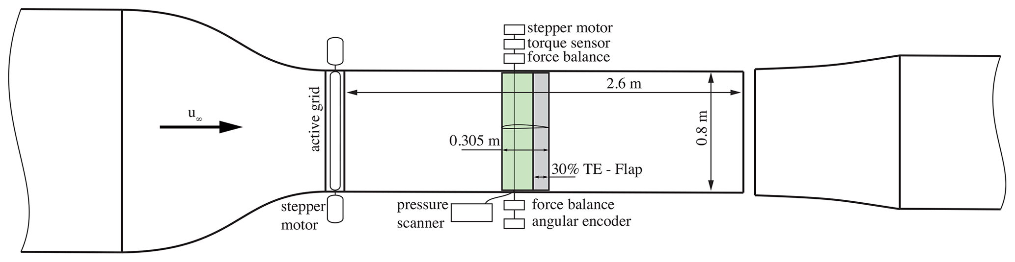
The inflow was modulated by a two-dimensional active grid (Wester et al., 2018). The grid consists of nine individual movable vertical NACA 0016 airfoils with a chord length of cgrid=71 mm and a span of sgrid=800 mm. Every vertical axis was turned by a single stepper motor, which enabled individual movements of the axes and therefore the generation of very complex but two-dimensional inflows. In the present study the seven inner axes performed a sinusoidal movement, whereas the two outer axes were used to increase or decrease the blockage. With this movement strategy a fairly sinusoidal angle of attack variation was generated by the inner axes, and the outer axes additionally imposed a streamwise sinusoidal gust. By changing the phase of the inner and outer axes, the angle of attack and streamwise velocity fluctuations were either in phase or out of phase.
The wing was mounted vertically on top of a turntable in the middle of the test section 1.1 m downstream of the active grid. The geometric angle of attack αturntable of the airfoil was controlled by a stepper motor, which was located on top of the test section. αturntable was kept constant during the measurements. Force measurements were realized by two force gauges of type K3D120 (ME-Meßsysteme), one at the top and one on the bottom of the airfoil, and a torsion sensor type TS110 (ME-Meßsysteme).
2.2 Wing with trailing-edge flap
In reference to the BeRT experiment, a two-dimensional wing was designed (see Fig. 2). It is based on a Clark-Y airfoil that was slightly increased in thickness at the trailing edge for manufacturing purposes. The chord is c=0.305m and the span is s=0.8 m. The shell of the main body was manufactured from glass-fiber-reinforced plastic (GFRP) supported by an aluminum structure. A solid, 3D-printed trailing-edge flap with a chordwise extension of 30 % was hinged by a fiber-reinforced polymer hinge.
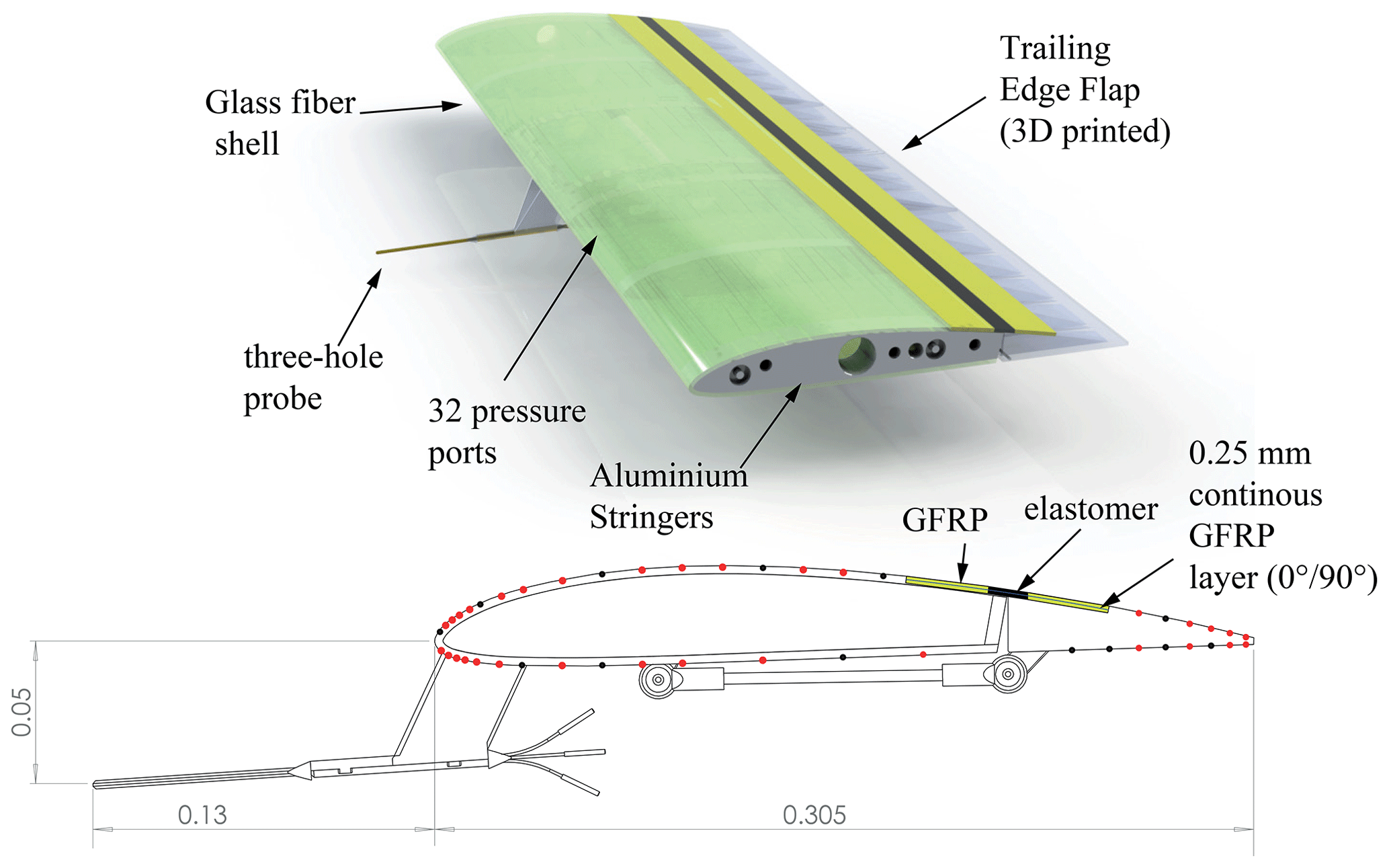
Figure 2Sketch of the employed wing. Red dots on the surface indicate employed pressure ports; black dots show ports that were not used.
Concerning the flap material and its connection to the main body, different literature examples were analyzed. As found in a CFD study by Troldborg (2005), a rigid flap is aerodynamically slightly less efficient than a flexible curved flap. Hence, for the same change in lift, a higher deflection angle is necessary. Furthermore, Buhl et al. (2005) indicated that an abrupt change in the surface geometry of an airfoil may lead to increased noise. However, a deflectable flap, made for example from rubber material, might show limits in fatigue lifetime on full-scale turbines, as their structural integrity might be compromised by environmental conditions, such as UV light. Employing piezo actuators that bend the wing surface requires a high voltage, and they are therefore unlikely to be used on lightning-exposed machines, such as wind turbines. Therefore, the current setup is based on a rigid flap, which could be built from GFRP in full-scale applications, and a continuous hinge. Thereby, a smooth surface on the suction side is achieved, which ensures that the aerodynamic performance and the structural integrity of a potential full-scale application are not affected.
The hinge is made of woven glass fiber fabric, epoxy resin, and elastomeric material and thus meets the lightning protection requirements of potential full-scale applications, as no metallic parts are contained. The flexible zone in the midsection of the hinge contains a 0.25 mm thin layer of GFRP to improve the hinge structures' in-plane stiffness and fatigue behavior while still maintaining sufficient flexural freedom. Moreover, this thin GFRP layer provides a more homogeneous deflection curve of the joint area, compared to unreinforced elastomer. In order to prevent buckling or buckling-related damages of this thin laminate, both surface areas were covered by 0.5 mm thick elastomer. Within a bending fatigue experiment an equivalent hinge was tested with over five million load cycles without showing any damage to the structure.
The flap was driven by a Faulhaber 32A servo motor located inside the wing. The connection to the trailing-edge flap was realized by a lever arm located outside of the pressure side (Fig. 2).
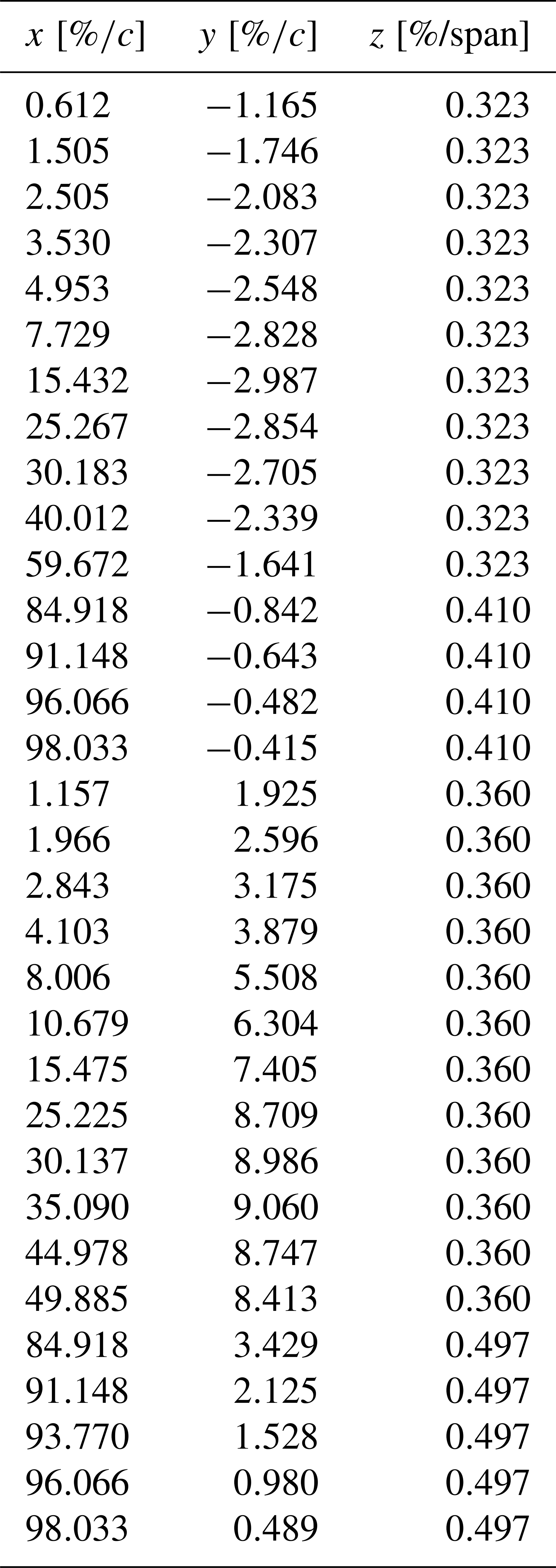
The final setup is shown in Fig. 3. On the left side, the pressure side is seen with the servo motor, three-hole probe and surface pressure ports. Note that, due to manufacturing limitations, not all pressure ports are in the same spanwise position. The diameter of the holes is 0.7 mm, and their coordinates are given in Table B1. On the right-hand side in Fig. 3 the suction side is depicted. The view is from downstream to upstream, thereby showing the inflow grid. Furthermore, the continuous hinge is shown as well as the trailing-edge flap.
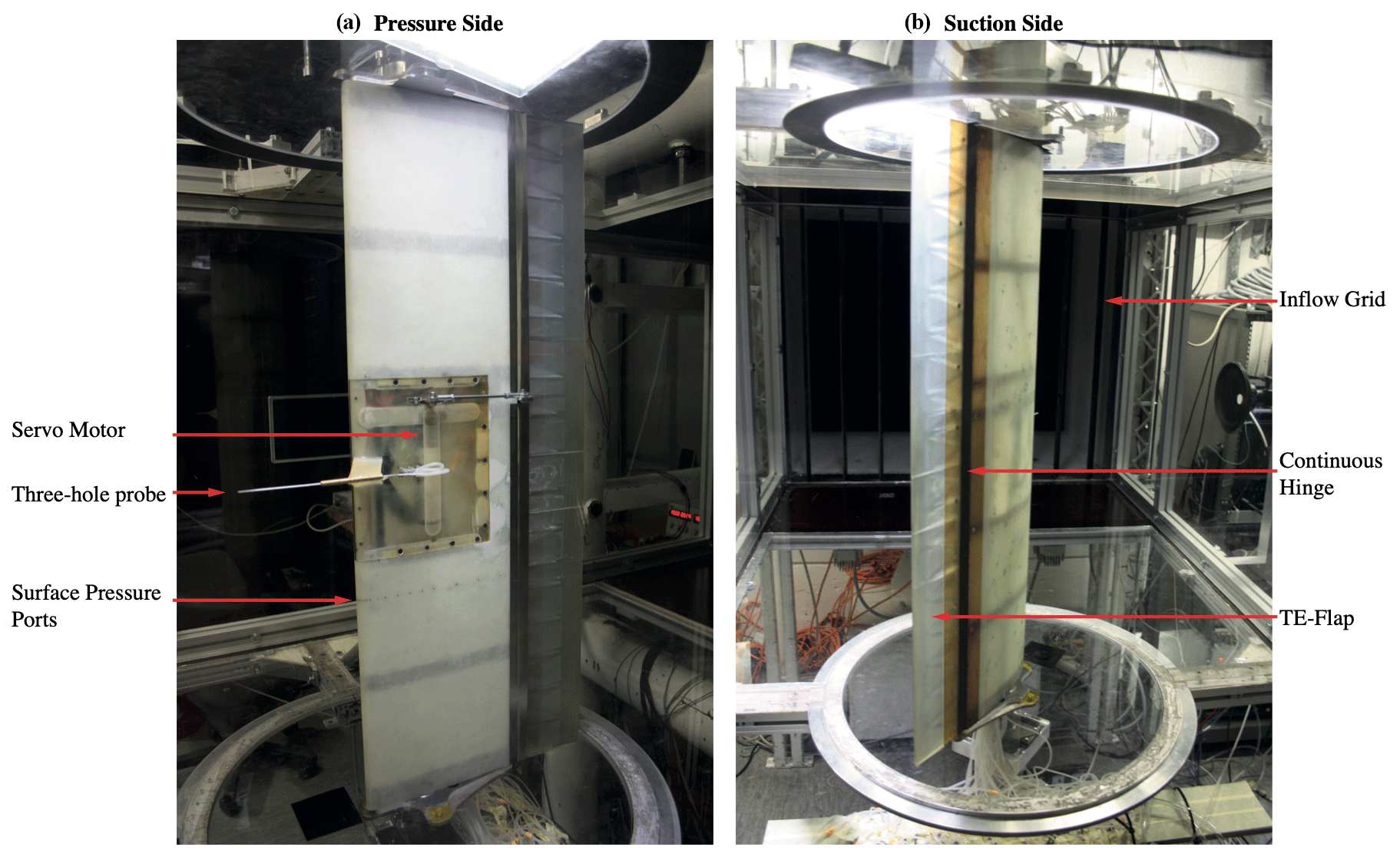
Figure 3Mounted wing inside the wind tunnel. (a) Pressure side. (b) Suction side; view from downstream to upstream.
2.3 Measurement hardware
Measurements were conducted using a National Instruments cRIO-9068 data acquisition system employing three analog-in NI 9220 modules. The acquisition frequency was set to fs=2 kHz. The cRIO also sent the position commands to the servo motor via the EtherCAT protocol at an update frequency of fupdate=100 Hz. The uncertainty of the sensors is summarized in Table 1.

The wing surface, including the trailing-edge flap, was equipped with a multitude of pressure ports. During the measurement campaign 32 ports were measured, which are shown as red dots in Fig. 2. Furthermore, the wing was equipped with a custom-made three-hole probe (Fig. 3) that was previously used on the model wind turbine BeRT (Klein et al., 2017; Bartholomay et al., 2018). The two outer tubes have a 45∘ chamfer angle, whereas as the inner tube has a chamfer angle of 0∘. The probe was employed to obtain the angle of attack and the inflow velocity. The underlying methodology is explained in Sect. 3.1.
The three-hole probe and the surface pressure ports were connected by 0.5 m tubing to the sensors. The reference static pressure was obtained from two wall-mounted pressure ports. These ports were located just upstream and in the center of the two innermost inflow axes of the active grid. This was necessary, as the original ring circuit for static pressure measurements was substantially affected by the changing adverse pressure created by the moving grid.
2.4 Frequency analysis of the test rig
The study presented in this paper is considered an aerodynamic and not an aeroelastic experiment. Therefore, the test rig was analyzed for its structural eigenfrequencies. The excitation for this task was driven by the trailing-edge flap. Multiple runs at various fixed frequencies were conducted, and time series of the force and torque balance were measured for each run. Each time series was Fourier transformed and the results were stacked, yielding waterfall diagrams (Figs. 4 and 5). The diagrams are comparable to a Campbell diagram, whereas for the current test rig the flap motion is used for excitation and not a rotational frequency as done for rotating machines. In Fig. 4 the result for the measurement of the moment is shown; the normal force is depicted in Fig. 5. The y axis depicts the set actuation frequencies, and the x axis corresponds to the Fourier transform of the signal. Diagonal lines represent the actuation frequency and its multiples, with the leftmost line corresponding to the actuation frequency. As can be seen for the moment, there is a significant response at 16.6 Hz, which is expected to be the torsional eigenfrequency of the test rig. This frequency appears also in the plot for the normal force. Additionally, a strong response can be seen at 24.8 Hz, which is expected to correspond to the normal eigenfrequency.
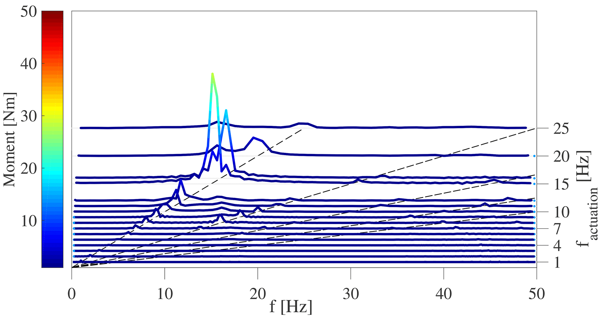
Figure 4Waterfall diagram of the moment at different actuation frequencies for the trailing-edge flap (y axis). The experiment was conducted with the tunnel speed set to .
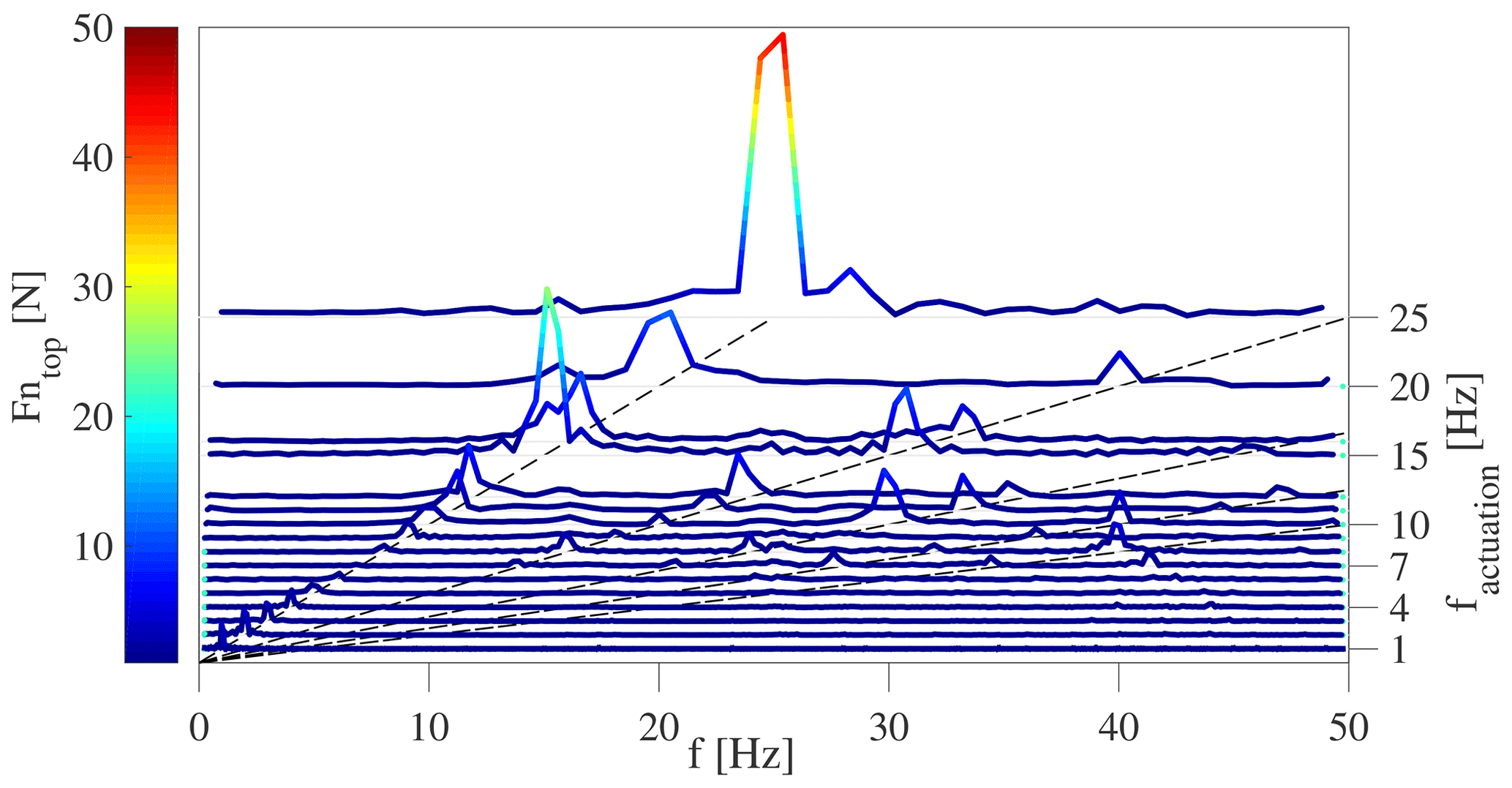
Figure 5Waterfall diagram of the normal force at different actuation frequencies for the trailing-edge flap (y axis). The experiment was conducted with the tunnel speed set to .
Furthermore, due to the acceleration of the flap inertia, a force which is opposite in sign to the aerodynamic lift created by the flap is created. Therefore, the force balance measures a zero lift amplitude where these two forces are equal. In the current setup this frequency is at 7 Hz.
2.5 Steady lift polars
Furthermore, the wing was tested for its baseline aerodynamic performance by measuring steady polar curves. For this purpose, the wing was turned by the turntable, and the inflow grid was kept in its neutral position. Multiple repetitions with constant flap angles from to in steps of were conducted. The results of the measurements are depicted in Fig. 6, where the dashed lines correspond to the balance measurements. Additionally, the full pressure port integration is given as solid lines.
The slope of the lift polars in the linear range remains constant for all flap deflections (Fig. 6). A positive flap deflection (flap turned towards pressure side) leads to a higher lift and vice versa. Furthermore, the angle of attack that corresponds to the lift maximum α(CLmax) is reached decreases when the flap angle is increased. Generally, the balance measurements show a fairly constant level of lift beyond α(CLmax) for the Clark-Y airfoil. At all lift polars achieve almost the same lift, whereas beyond this point the differences increase again. However, the trend of higher lift due to higher positive flap deflection remains.
The lift curves based on the full pressure port integration show a slightly steeper slope, which is to expected, as the measurement is at selected spanwise positions only and not integrated over the full span. The latter might be corrupted by corner effects.

Figure 6Steady polar curves. Comparison between force balance (dashed lines) and full pressure port integration (solid lines). Error bars correspond to the standard deviation. Furthermore, the XFOIL calculation is shown as the solid black line.
As this study focuses on load control to achieve constant lift, the lift slope in the linear region is most important (d). Moreover, the flap-lift slope is calculated to d, which results in a flap effectiveness of . The former two values are used in the pressure-based lift estimation methods to predict the current lift. Furthermore, the flap effectiveness is necessary to calculate the flap set point within the feedforward controllers.
The current load control concept is based on pressure-based lift estimation. Therefore, the two employed methods are presented in this section. The first method relies on a three-hole probe and the second method on surface pressure ports.
3.1 Estimation procedure based on three-hole probe measurements
The first lift estimation method is based on a three-hole probe that is located at upstream of the leading edge. The measurement at this position is influenced by the induction of the blade. Therefore, a correction method based on quasi-steady assumptions to eliminate the induction effect was developed by Bartholomay et al. (2017) and compared to an URANS solution by Klein et al. (2017) for the rotating test rig BeRT. This method is extended in the present study to include the change in induction for different trailing-edge flap angles. A flowchart of the method is shown in Fig. 7, and the corresponding sketch is given in Fig. 8.
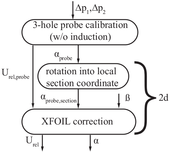
Figure 7Flow chart for the estimation of angle of attack and velocity from three-hole probe measurements (adapted from Klein et al., 2017).
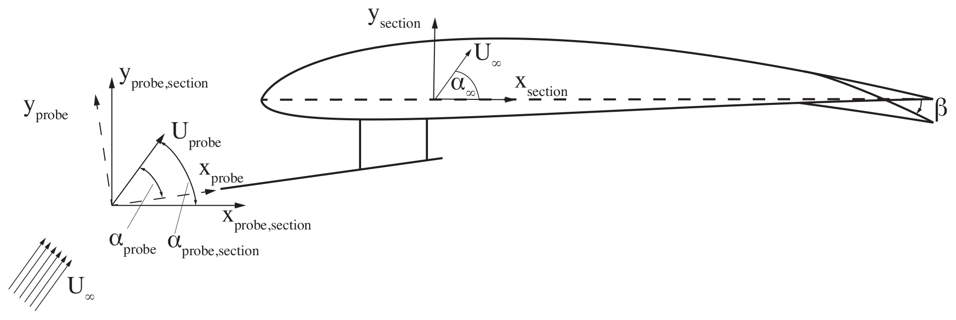
Figure 8Sketch for the estimation of angle of attack and velocity from three-hole probe measurements (adapted from Klein et al., 2017).
The three-hole probe lift estimate (3HP estimate) relies on two pressure sensors that each measure the pressure difference (Δp1,Δp2) between one of the outer holes and the reference hole in the middle of the probe. The pressure differences were calibrated in a separate probe-only wind tunnel experiment, within an AoA range of −30 to 30∘ for angular and velocity measurements. The calibration allows us to derive the αprobe and the velocity Uprobe in the experiment, as seen in the flow chart in Fig. 7. In a second step, the angular difference between the probe and the chord of the wing is taken into account. Thereby, the flow angle αprobe,section at the probe head is expressed in the section coordinate system. In the third step, XFOIL (Drela and Youngren, 2001) calculations are used in the current study to correlate the αprobe,section and Uprobe,section to the uninfluenced α∞ and U∞. These calculations are based on simulations from an AoA range of to 30∘ in steps of at flap angles of to 10∘ in steps of . Values in between these predefined AoA and flap angles are linearly interpolated. This last step is comparable to the procedure presented by Petersen et al. (2015) that is based on 2D CFD simulations. However, it is expected to be considerably less computational expensive.
Generally, as this method is based on XFOIL, it is a quasi-steady approach for lift estimation. Nonetheless, for low frequent disturbances this method seems promising and will be evaluated for feedforward control.
3.2 Estimation procedure based on three selected surface pressure ports
Due to their fragility, three-hole probes are rather used for research projects and are unlikely to be used as a permanent measurement instrument on industrial turbines. Therefore, a method is proposed that correlates three surface pressure measurements and the flap position to the angle of attack and velocity. The method is based on unsteady thin airfoil theory (Gaunaa, 2006). Gaunaa and Andersen (2009) and Velte et al. (2012) apply the original work in order to estimate the unsteady lift based on the pressure difference of two pressure ports at on the suction and pressure side. However, implicitly within this application of the theory, it is assumed that the local inflow velocity is known. On large turbines, the relative velocity can be estimated from the current rotational speed, hub height measurements of velocity, assumptions of the atmospheric boundary layer and the azimuthal position. However, local flow differences cannot be estimated from such a global approach.
Therefore, an approach is needed that estimates the local inflow velocity. This was done in other experimental studies before. For example Shipley et al. (1995) used a complete pressure port distribution around the airfoil to extract the velocity from the stagnation pressure. The stagnation point was found by searching only for the maximum pressure of the pressure distribution. The disadvantage of such a method is a high number of pressure ports that is necessary to achieve a good resolution at the leading edge.
Thus, an approach that employs one additional pressure port at the leading edge to estimate the inflow velocity is presented. The remainder of this section presents the derivation of the inflow velocity first and secondly the derivation of the unsteady lift. A flow chart of the current method is given in Fig. 9.
In the current study, one single additional pressure port on the pressure side at is used, in combination with the pressure ports at on the suction and pressure side, to estimate the inflow velocity. The approach is based on steady polar data, which are taken at the velocity of , and an AoA range of in steps of and flap angles ranging from to 10∘ in steps of .
From the static polar data, the normalized pressure difference is obtained:
and
Ignoring effects of changing Reynolds numbers, the dimensionless pressure differences are multiplied by the velocity range of U∞=10 to 25 m s−1, yielding
and
Thereby, a lookup table, given for a flap angle in Fig. C1, is created, which relates the velocity to a function of the two pressure differences and the flap angle:
During the measurements, the velocity estimation feeds directly into the procedure of the lift estimation shown in Fig. 9.

Figure 9Flow chart for estimation of the unsteady lift based on selected surface pressure measurements.
In a second step, the unsteady lift is estimated based on the derivation of Gaunaa and Andersen (2009) and Velte et al. (2012). This method relies on the calculation of the effective AoA, which corresponds to the effective three-quarter AoA containing the bound and shed circulation. The effective AoA is derived from the pressure difference between the suction and pressure side, according to Gaunaa and Andersen (2009):
where gc(x) corresponds to the circulatory pressure difference distribution, gcamber(x) corresponds to the pressure difference coefficient due the camber of the airfoil and gβ(x) represents the pressure difference coefficient due to the deflection of the trailing-edge flap. The last two terms in Eq. (6) are denoted by Gaunaa and Andersen (2009) as added mass effects. Note that these are not related to added mass effects due to airfoil, flap or flow motion. Yet, they signify the change on the pressure distribution that is introduced by the fact that the camber line is not straight but cambered and eventually further deflected through the current flap position. is the pressure difference function due to pitching motion, which is shown from thin airfoil theory to be zero at . The last term in Eq. (6) corresponds to higher-order terms. An approximate pressure difference is found by neglecting the latter, using the pressure difference at and neglecting the pitch rate term as done by Gaunaa and Andersen (2009), which yields
The constants K1, K2 and K3 are derived from the static polars, and αeff yields
The effective angle of attack is then inserted into
where kc corresponds to the steady lift slope and to the added mass term due to airfoil motion. The latter is given as in Gaunaa and Andersen (2009). Following Velte et al. (2012) and Gaunaa and Andersen (2009), the lift coefficient can be approximated by neglecting the added mass term. Thereby, an estimation of the unsteady lift is given, which does not include added mass effects due to changes in AoA or flap motion. Experimentally this method was employed by Velte et al. (2012) for a NACA 64418 airfoil with an active trailing-edge flap. Finally, the lift is calculated from equation
where the inflow velocity was taken from the estimate conducted in the first step.
The presented pressure-based lift estimation methods are used in a static feedforward control approach to alleviate fluctuating loads. Feedforward control has the advantage that controller action can be taken before the error is experienced by the system (Åström and Murray, 2008). In this particular case the trailing-edge flap can be actuated before the balance measures a change in lift. Therefore, the disturbance has to be measured earlier by an alternative sensor (pressure-based AoA and velocity measurement in this case), and good process models (lift estimation) have to be present. The drawback of feedforward control is that model and measuring uncertainty cannot be controlled. In the present study, two feedforward controllers are compared to a PID-based feedback controller.
For each controller setting the same low-pass filter setting is used. The cut-off frequency was set to fcut-off=7 Hz as the mechanical setup of the flap leads to negative lift responses beyond the cut-off frequency due to the acceleration of the flap inertia, as explained in Sect. 2.4. The low-pass filter introduces a loss of gain and a phase shift that is expected to lower the capability of the setup. In order to keep the same filter setting for all controller types, a low-pass filter and not a band-pass filter was chosen. Furthermore, the update frequency of the controller loop is fupdate=100 Hz.
4.1 Feedback controller
In Fig. 10, the feedback controller is shown. It is important to note that the lift was taken from the force balance measurement. The reference lift is found by taking a 10 s mean from the current lift, without the disturbance being active. The PID constants for the operating point of were chosen based on the standard Ziegler–Nichols method by increasing Kp until self-oscillation. The resulting PID values are Kp=0.54, Ti=0.009722 min and Td=0.
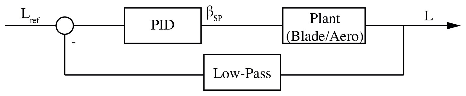
Figure 10Feedback PID controller based on lift measurements of the force balance. Reference lift is based on a 10 s mean at constant inflow conditions. βSP denotes the set point of the flap. The system plant comprises the flap mechanics and the aerodynamics.
4.2 Feedforward control based on the three-hole probe
The controller based on the three-hole probe, denoted as the 3HP controller, is shown in Fig. 11. The first block from left indicates the calculation of the angle of attack and velocity as given in Fig. 8. Additionally, taking the current flap position into account, the lift is calculated. After low-pass filtering, the lift is subtracted from the reference, which is also taken from the 3HP estimate of the lift. Note that for a fair comparison the low-pass filter was chosen with the same settings as for the feedback controller. Finally, the flap set point βSP is determined by the use of the slope given by the static lift polars (see Fig. 6).

Figure 11Feedforward controller based on the three-hole probe lift estimate. The first two blocks corresponds to the lift estimation presented in Sect. 3.1. The flap angle set point is calculated based on the error in reference to a 10 s mean. The latter is also based on three-hole probe measurements.
4.3 Feedforward control based on three surface pressure ports
Figure 12 shows the second feedforward controller (PP controller), which is based on the surface pressure port lift estimate. The only difference in comparison to the 3HP controller consists of the lift estimate, which is based on the surface pressure ports described in Sect. 3.2. The same low-pass filter setting was also chosen for this controller.
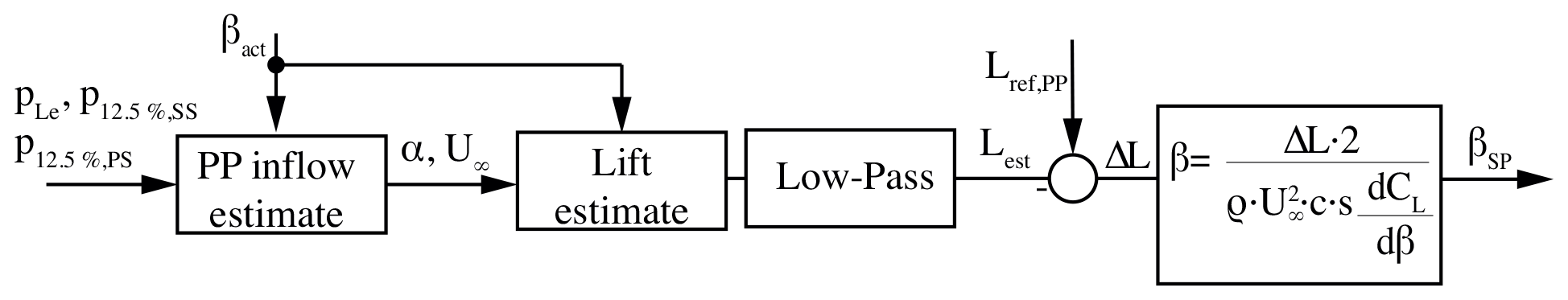
Figure 12Feedforward controller based on surface pressure port measurements. The first two blocks corresponds to the lift estimation presented in Sect. 3.2. The flap angle set point is calculated based on the error in reference to a 10 s mean. The latter is also based on surface pressure port measurements.
To allow for a consistent evaluation of each control method, different metrics are employed.
Plumley (2015) gives a detailed overview of different fatigue load metrics, starting with the standard deviation of time series, cumulative power spectral densities (CPSDs) and (short-term) damage equivalent loads (DELs). Whereas the standard deviation is a quick way to compare fluctuating loads, it does not give any information on important frequencies in the time series. Therefore, CPSDs are useful, as they shed light on the frequencies that contribute most to the signal energy. Additionally, it is useful to calculate DELs as they provide a concise and representative number of the loading scenario. The latter two metrics are employed in the current paper and are therefore explained in the following two sections.
5.1 Cumulative power spectral density
The explanations in the current section follow Plumley (2015). Power spectral density plots are used to find frequencies which contain the most energy and thereby where the most damage is created. The calculation in this paper is based on Welch's power spectral density, which is then cumulated to highlight dominant components. These components can be seen as steps (see for example Fig. 21), which facilitate the comparison between the baseline and the controlled signals.
5.2 Short-term damage equivalent loads
Damage equivalent loads are a standard metric in the wind energy industry. They are calculated in the time domain and take the material fatigue into account. In the current study only short term DELs are calculated in order to compare different time series to one another. The time series are low-pass filtered at a cut-off frequency of f=15 Hz, which corresponds to the first eigenfrequency of the test rig, before DELs are calculated.
The calculation of DELs was performed using the NREL (2015) MLife code, which is publicly available. Hayman (2012) describes in the accompanying report the procedure to process the DELs, which is explained here briefly. The calculation is based on rain-flow counting of load cycles in the time domain, resulting in cycle counts ni for different loading amplitudes Li. Based on Miner's rule, which assumes linear accumulation of damage di at different loading, the total damage is given as
where Ni(Li) describes the number of sinusoidal cycles to failure for each specific loading amplitude, which is found by employing Wöhler (S–N) curves. Furthermore, the total damage calculated in Eq. (11) is expressed by one equivalent load (DEL) at a chosen number of cycles neq. In order to find the DEL, the Wöhler exponent m is needed, which is chosen as m=10 for composite material in the present study. The ultimate load Lult technically needed for Wöhler (S–N) curves cancels out in the derivation. Thereby, Eq. (11) yields
In order to calculate the DEL, the equivalent frequency is chosen as feq=1 Hz. Thereby, the equivalent number of cycles is found by , where T is the elapsed time of the time series. By rearranging Eq. (12), the damage equivalent load is found:
Summarizing, comparing signals for their success of load alleviation, it is important to look at different methods. Employing CPSDs is important to reveal what frequencies are affected, but they might falsely suggest a controller superiority where there is none. Therefore, DELs are necessary to quantify damage over all frequencies and to assess the effect on the component.
In order to assess the lift estimation methods, three scenarios with increasing complexity are analyzed: active flap motion with constant inflow, fixed flap with inflow disturbance and active flap with inflow disturbances. The aim is to assess the limits of the presented methods. Therefore, the reduced frequencies range up to fairly high values even though they might have limited interest for the wind energy community.
6.1 Constant inflow conditions – active flap
The quality of lift estimation is analyzed first in test cases where the AoA is set to , and the inflow velocity is kept constant at U∞=15 m s−1. The flap executes a sinusoidal motion with an amplitude of and at a fixed frequency. The results of the analysis are shown in Fig. 13, and a zoom on the frequency range of up to f=7 Hz is given in Fig. 14. Both diagrams show the phase and the gain of the complex transfer function between the flap set point signal and the lift measurements (balance and full surface pressure integration) or the presented lift estimation methods. For the calculation of the gain a steady lift equivalent served as a reference. This is considered the lift that would be achieved if the flap were to settle at the set point amplitude and the lift were to reach its corresponding steady value:
The flap actual position (Fig. 13, black line) corresponds to the ratio between the amplitude of the actual flap amplitude and the set point amplitude. Furthermore, LBalance corresponds to the lift force deduced from the balance measurements and LFULLPP to the calculated lift based on the integration of the lift over the complete set of pressure ports. L3HP and LPP show the result of the three-hole probe and three-surface-pressure-port method, respectively. Additionally, the unsteady aerodynamic model ATEFlap (Bergami and Gaunaa, 2012) was used for comparison. In order to account for the non-zero thickness of the airfoil, the indicial constants for the model are calculated in reference to Bergami et al. (2013) and slightly adjusted: and . The deflection shape integrals are calculated for the flap with a chordwise extension of 30 % according to Gaunaa (2006, Eqs. 39/40) and normalized by the half chord to , and .
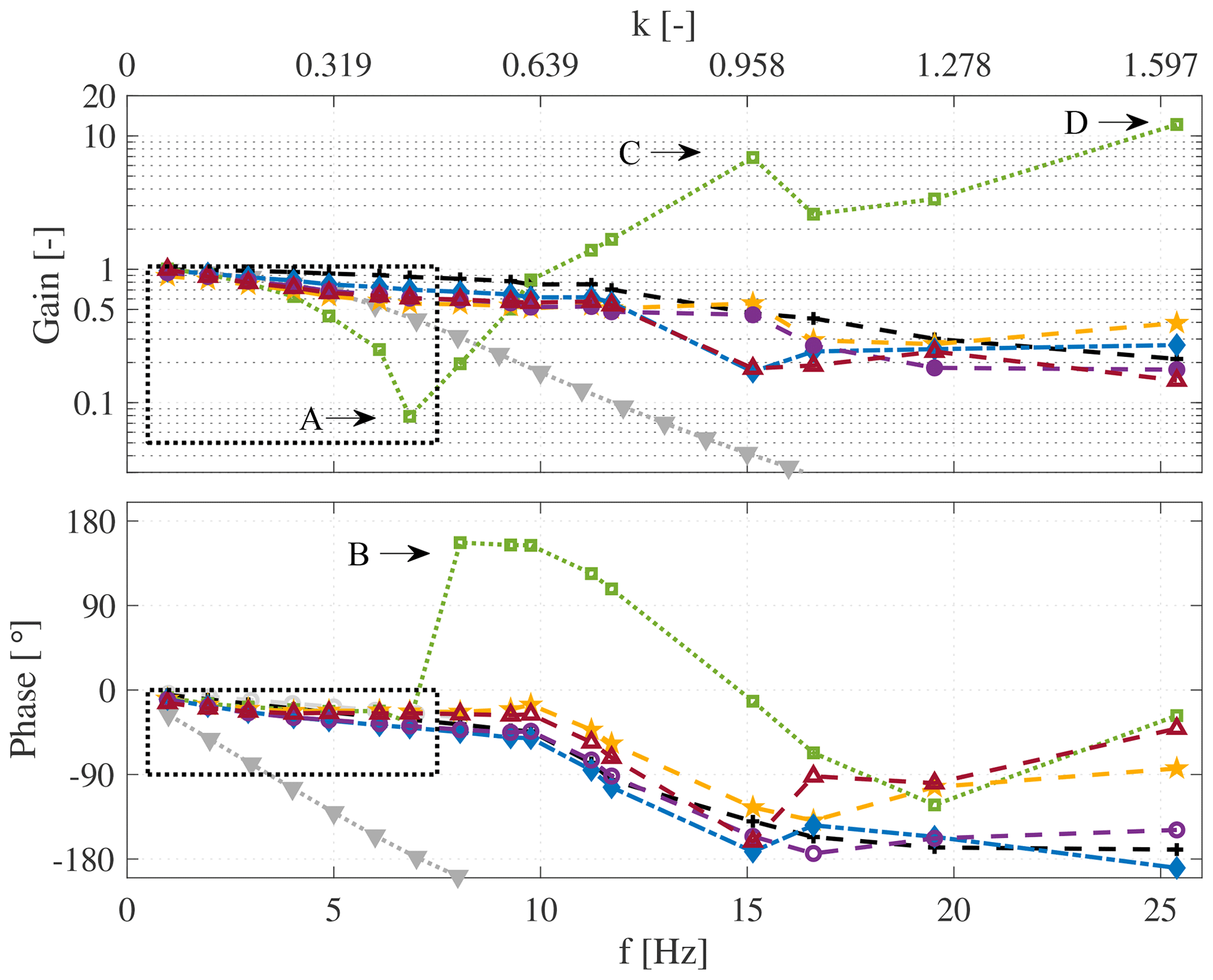
Figure 13Bode plot of the transfer functions. Gray lines correspond to the filter setting and update time of the controller loop. Black line: transfer function from flap set point βSP to flap actual position βactual. All other lines correspond to βSP and to the lift measurements or lift estimates.
Concerning the flap motion, it can be seen in the upper plots in Fig. 13 (black line) that the flap follows its set point signal up to 10 Hz with little lost on the gain. Beyond this point, the amplitude decreases to 21 % at the frequency of f=26 Hz and the phase drops to . This indicates that the present mechanical setup shows a decent functionality up to a frequency of f=10 Hz. At higher frequencies the introduced phase lag and the small gain poses a high challenge for load alleviation applications.
Considering the lift measurement of the balance LBalance (Fig. 13 green line), it is seen at marker A that the gain decreases to 8 % at f=7 Hz. This is caused by the acceleration of the flap inertia that creates a force amplitude which is phase shifted 180∘ to the flap position. After the minimum is reached, the gain raises again, as the flap is accelerated faster with increasing frequency, and thereby the force created by accelerated flap inertia dominates the lift response. At f=9 Hz the gain of the other measurements is reached but with leading phase. The gain keeps increasing further with increasing frequency, and in point C and D eigenfrequencies of the test rig are hit, as shown in Sect. 2.4. This leads to enormous gains, which are not related to the flap motion only, nor are they representative of the acting aerodynamic forces.
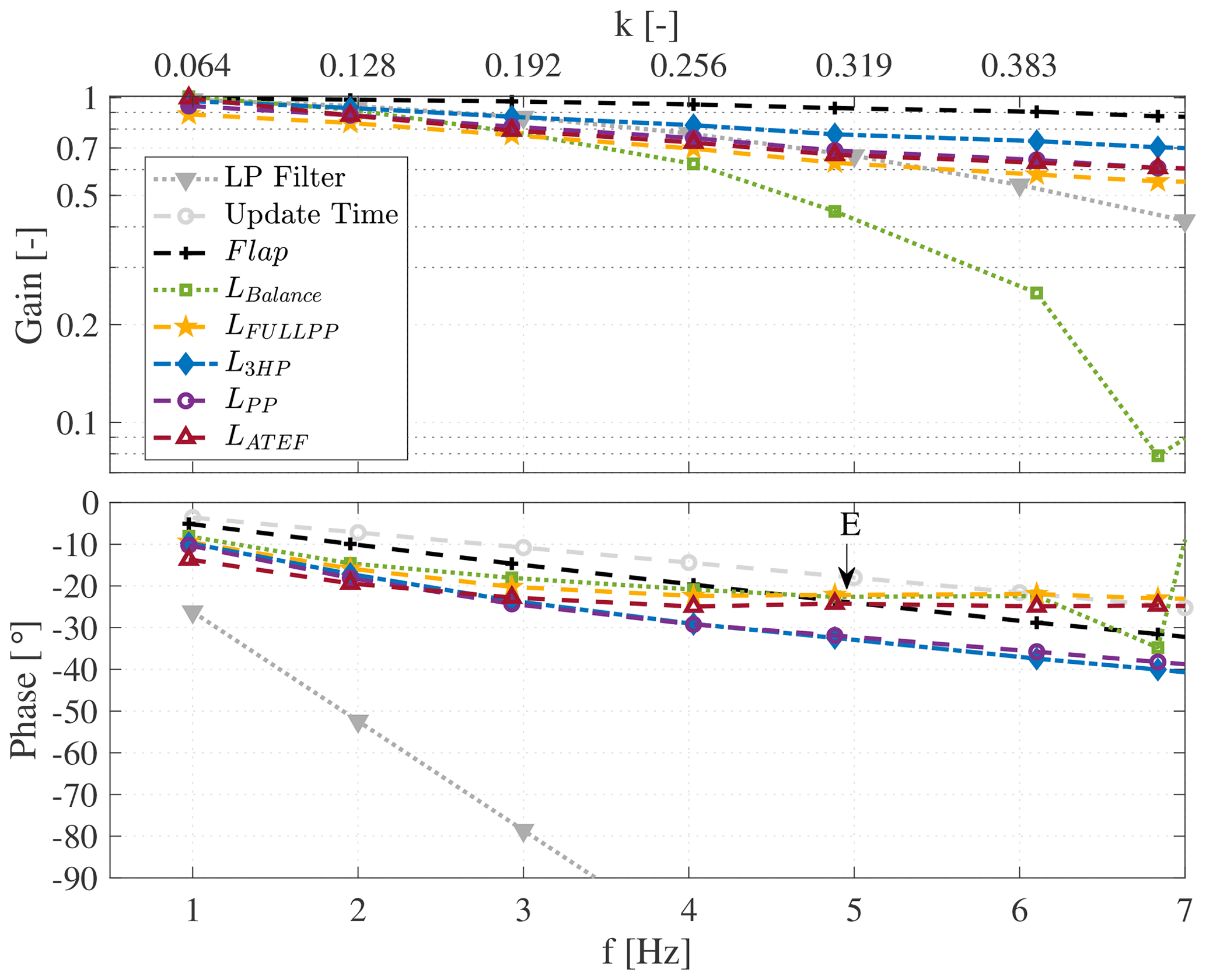
Additionally, the lift is measured based on the integration of the complete pressure port set distributed on the surface of the wing (Fig. 14 yellow line – LFullPP). It is seen that the lift does not drop as indicated by the balance measurements, which is plausible, as the flap inertia is not measured by the pressure ports. However, added mass effects are measured by the integrated lift and by the balance measurements, which is seen in Fig. 14 at point E where the phase of the lift measurement becomes greater than the phase of the flap actual position. This point is denoted as the phase turning point and is discussed later in this section.
Concerning the phase of the three-hole probe (Fig. 14 blue line) and the surface pressure port estimate (purple line), it can be seen that up to a reduced frequency of k=0.19 the phase difference to the integrated lift is small. However, beyond this point the phase error increases, as added mass effects are not taken into account in the lift estimations. Note that in the case where only the flap is moving and no inflow disturbance is present, the lift estimates lag the integrated lift in phase. This is expected due to the location of the probes ( for the three-hole probe and for the pressure ports) and the fact that the change in circulation is created due to the trailing-edge flap motion. This change in circulation alters the flow field around the airfoil; however, the change is introduced at the trailing edge. Thus, the three-hole probe is lastly affected in reference to the other methods.
In order to understand the phase turning point seen at marker E in Fig. 14, the lift hysteresis loops, CL over β in this case, are investigated in Fig. 15. The phase turning point becomes apparent by the change in direction of the loops from counterclockwise to clockwise. Starting from the reduced frequency of k=0.065 to k=0.130 the counterclockwise loop gets wider first, indicating the increasing effect of unsteady aerodynamics and hence the wake memory effect that leads to a delayed lift response to the change in flap motion. However, beyond k=0.130 the loop closes again and is virtually a straight line at k=0.324. Increasing the frequencies further leads to a reopening of the loop; however, the direction of the loop changes due to added mass effects. The effect of phase turning happens at the reduced frequency of k=0.318 (Fig. 14 marker E), which is higher than the phase turning point of k=0.144 as reported by Motta et al. (2015). However, the latter concerns an airfoil pitching case, where the accelerated mass is substantially larger in comparison to the current case where only the flap is moving. The balance measurements and integrated lift were compared to the ATEFlap model, and the phase turning point between the two measurements and the model agrees well (Fig. 14 marker E).

Figure 15CL over actual flap angle for increasing frequencies. The arrow indicates the sense of rotation of the loop. Up to the frequency of k=0.259 the sense is counterclockwise, and it is clockwise for higher frequencies.
6.2 Disturbed inflow conditions with fixed and active flap
Within the second and third test case the wing was exposed to inflow disturbances at a mean AoA of with fixed and active trailing-edge flap motion.
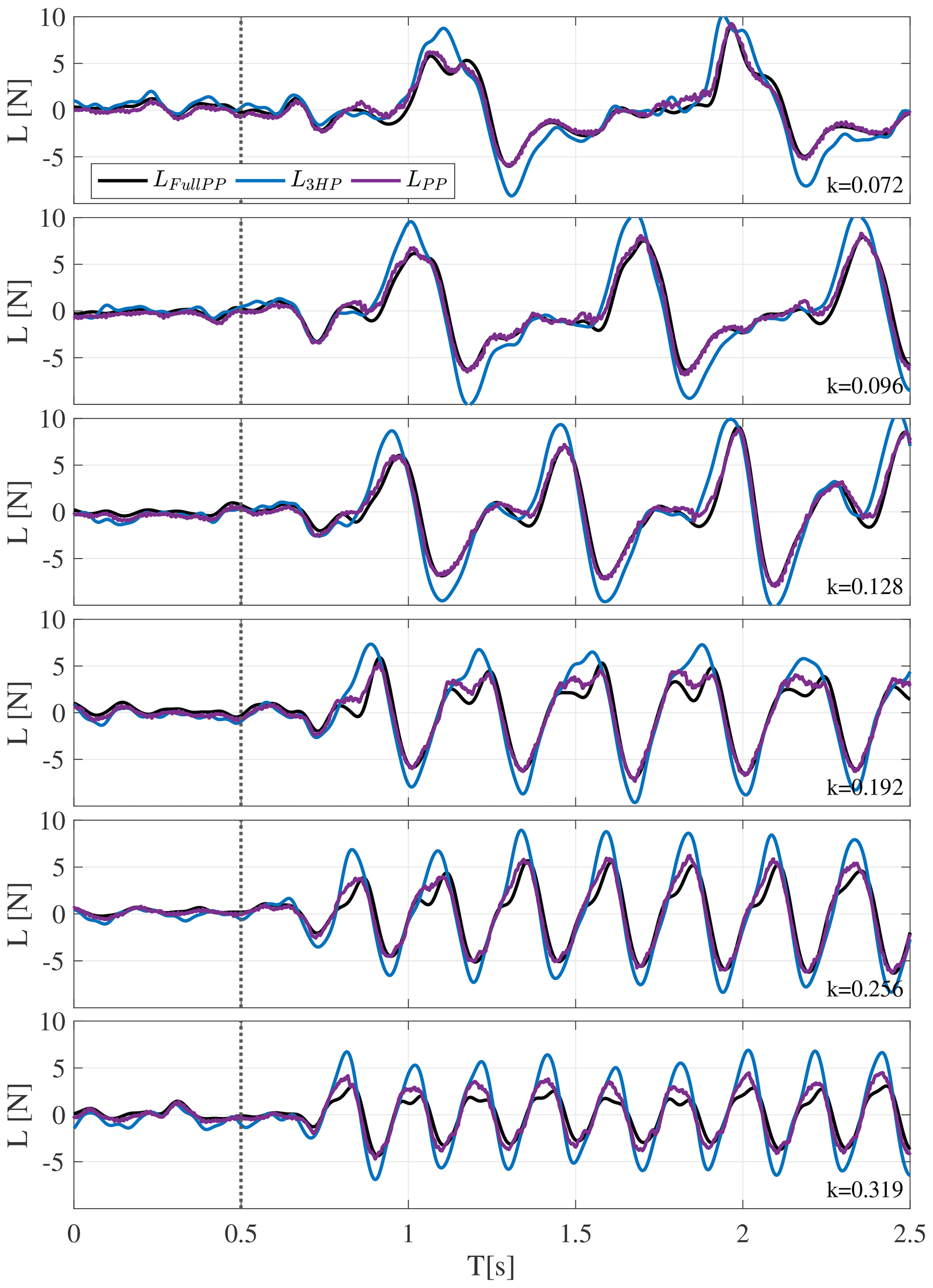
Figures 16 and 17 show time series of the lift when the wing is exposed to disturbed inflow conditions. Figure 16 depicts test cases in which the trailing-edge flap is fixed in its neutral position. The diagrams depicted in Fig. 17 correspond to test cases where the flap is active. The different rows correspond to the different disturbance frequencies in ascending order. In each plot the comparison between the previously presented estimation methods and the lift measurement based on the integration of the complete set of pressure ports LFULLPP is given. As can be seen for the fixed flap cases (Fig. 16), the comparison between the LFULLPP and the lift estimation based on three surface pressure ports LPP is fairly good up to a reduced frequency of k=0.256. At the highest frequency, k=0.319, the lift amplitude is slightly overestimated.
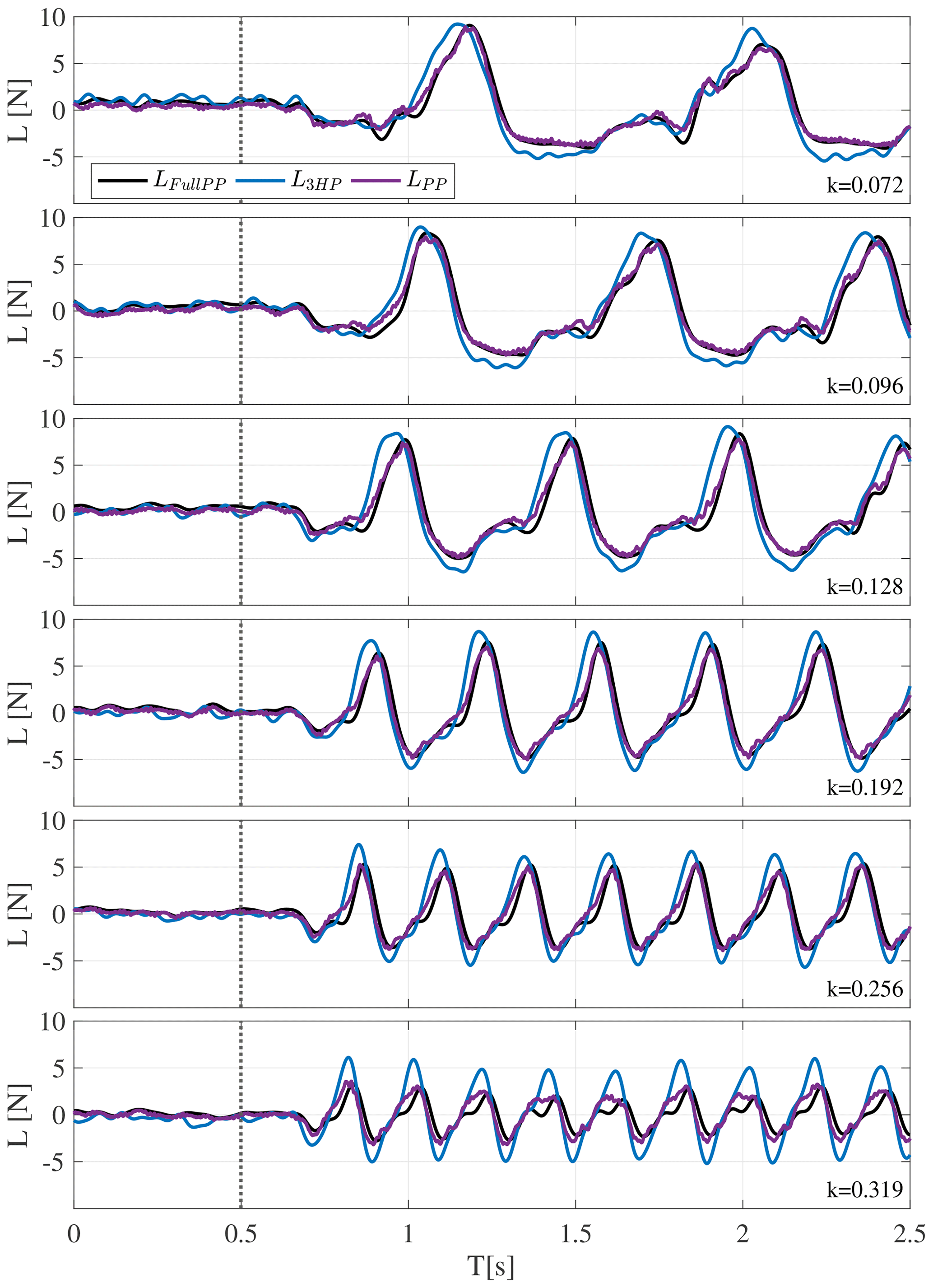
Considering the same estimation method, LPP for cases with actively moving flap (Fig. 17), the trend is generally kept; however, the differences are slightly larger in comparison to the LFULLPP. Regarding the lift estimate based on the three-hole probe L3HP, it can be seen that the lift amplitude is overestimated in all cases. Due to the lack of incorporation of unsteady effects into this method, this trend worsens with increasing frequencies. Furthermore, this method shows a significant phase lead in comparison to the full pressure result LFULLPP due to the position of the probe. This phase lead is beneficial for load control as is seen in Sect. 7.
In order to quantify the results of the lift estimation, the phase difference and the normalized root mean square deviation (NRMS) between the presented methods and fully integrated lift were calculated. The NRMS is given in the following equation:
where the time average is used for the root mean square. Figure 18 shows the results of the comparison, where the upper graph depicts the NRMS and the lower plot shows the phase difference. The latter is calculated by means of cross-correlation between the signals. The NRMS is calculated after alignment of the signals by the calculated phase difference.
Concentrating on the NRMS of the three-hole probe measurements for the fixed flap case first (see Fig. 18, upper plot), the deviation of this quantity stays fairly constant at about 10 % until a frequency of f=3 Hz and starts increasing from that point towards 40 % at f=5 Hz. This high error is to be expected, as wake memory effects and lift changes due to non-circulatory terms are neglected within this method. Considering an actively moving flap for the same case leads to an additional error of about 5 %, as additional unsteady effects which are not captured are present. Regarding the phase difference of the three-hole probe, a linear increase in the phase for the case of a fixed flap from to at a reduced frequency of k=0.319 can be seen (see Fig. 18, lower plot). This increase corresponds to a fairly constant time difference between the signals of about Δt≈0.02 s. This time delay may be converted to a convective distance of s≈0.3 m using the free stream velocity as the convection velocity. This value is close to the sum of the distance of the three-hole probe head and the half-chord length (). Hence, this time difference is most probably created due to the location of the probe's head.
Considering the active flap case, Fig. 18 shows that the phase of the three-hole probe measurements is lower than in the fixed flap case. Furthermore, the differences increase towards higher frequencies. This is expected to result from the flap motion, which leads to additional added mass forces that in turn create a phase lead as seen in Fig. 14. As added mass effects are not included in this method, a decrease in phase is created.
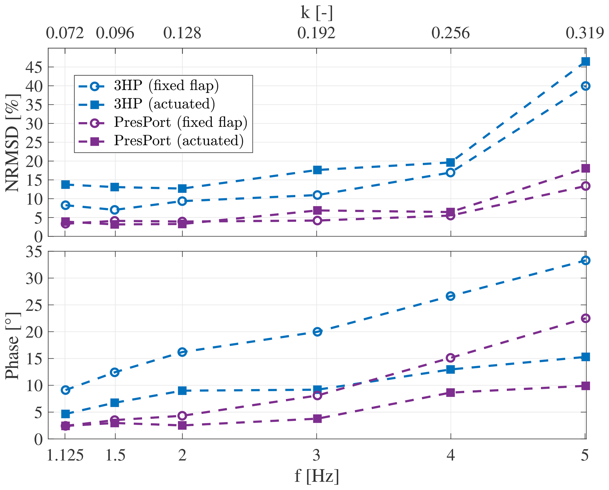
Figure 18Normalized mean root square deviation and phase difference between lift estimation methods and full pressure distribution results.
Concerning the pressure port lift estimate, the error is substantially smaller for all frequencies, and also the difference between the fixed and active flap cases is less significant. This is due to the fact that this method takes unsteady effects into account. The error increases towards higher reduced frequencies, which is again expected to happen due to the neglected added mass effects within this method. Finally, the phase difference for the pressure port estimate is substantially smaller in comparison to the three-hole probe results. This is primarily due to the location of the ports on the airfoil. Again, for the fixed flap case a linearly increasing phase difference is present. Regarding the measurements for the active flap cases, the phase difference is reduced, and also the difference to the fixed flap case increases with raising frequency. Furthermore, this is due to the fact that additional added mass effects due to flap motion are not taken into account in the surface pressure port method.
The presented lift estimation methods are employed as input to two separate feedforward control strategies. The performance of two feedforward controllers is compared to a standard PID feedback controller in the current section.
In Fig. 19, 10 s of the time series for the inflow disturbance at k=0.072 is shown. Herein, the angle of attack and velocity variation, measured by the three-hole probe, are shown in the first and second diagram. In the third graph, the flap motion is shown, and the resulting lift is depicted in the bottom diagram. The dashed gray vertical line in all graphs indicates the start of the inflow grid motion. In these diagrams, the baseline case and the different controller strategies are plotted on top of each other. For completeness, the time series for higher reduced frequency are given in Appendix D.

Figure 19Time series of AoA and inflow velocity variation, flap motion, and resulting lift amplitude at a reduced frequency of k=0.072 for different control methods in comparison to the uncontrolled baseline case.
As can be seen in the first two plots, the angle of attack and velocity variations, created by the inflow grid, are reproducible over time and between the different cases. Furthermore, the variations are periodic but not harmonic. The grid motion aimed at an in-phase disturbance between the angle of attack and velocity variation. The two properties are inherently changed by a moving grid in the wind tunnel: larger angles of attack leading to higher blockage, hence lower flow velocity. Therefore, an independent harmonic disturbance of angle of attack and velocity could not be established at the employed frequencies. Such disturbances are for example seen in yaw case situations on wind turbines (in this case, angle of attack and velocity variation are 180∘ out of phase) (Bartholomay et al., 2018, Fig. 20).
Nonetheless, the inflow disturbances are employed here as test cases for the controller configurations and are considered more challenging than pure harmonic disturbances. Furthermore, the shape of the inflow disturbances also vary when the frequency is changing, as seen in Appendix D. Therefore, each test case has to be analyzed separately. All quantitative results that are explained in the following sections are given in Table F1.
7.1 Inflow disturbance at a reduced frequency of k=0.072 (f=1.125 Hz)
The bottom graph in Fig. 19 shows the resulting lift variation for the test case at k=0.072. Distinct peaks are visible at the moment where the maximum angle of attack and the velocity maximum coincide (black line – baseline).
The lift then drops to a fairly constant plateau before picking up again. Fig. 19 (lower plot) clearly shows that all controller strategies accomplish a certain reduction of the lift maximum.
In order to analyze the success of the strategies in more detail, short-term damage equivalent loads (DELs) are calculated. The comparison of the DELs can be seen in Fig. 20. In this graph, results are normalized by the baseline DEL, corresponding to the wing exposed to inflow disturbances with fixed flap at each analyzed frequency.
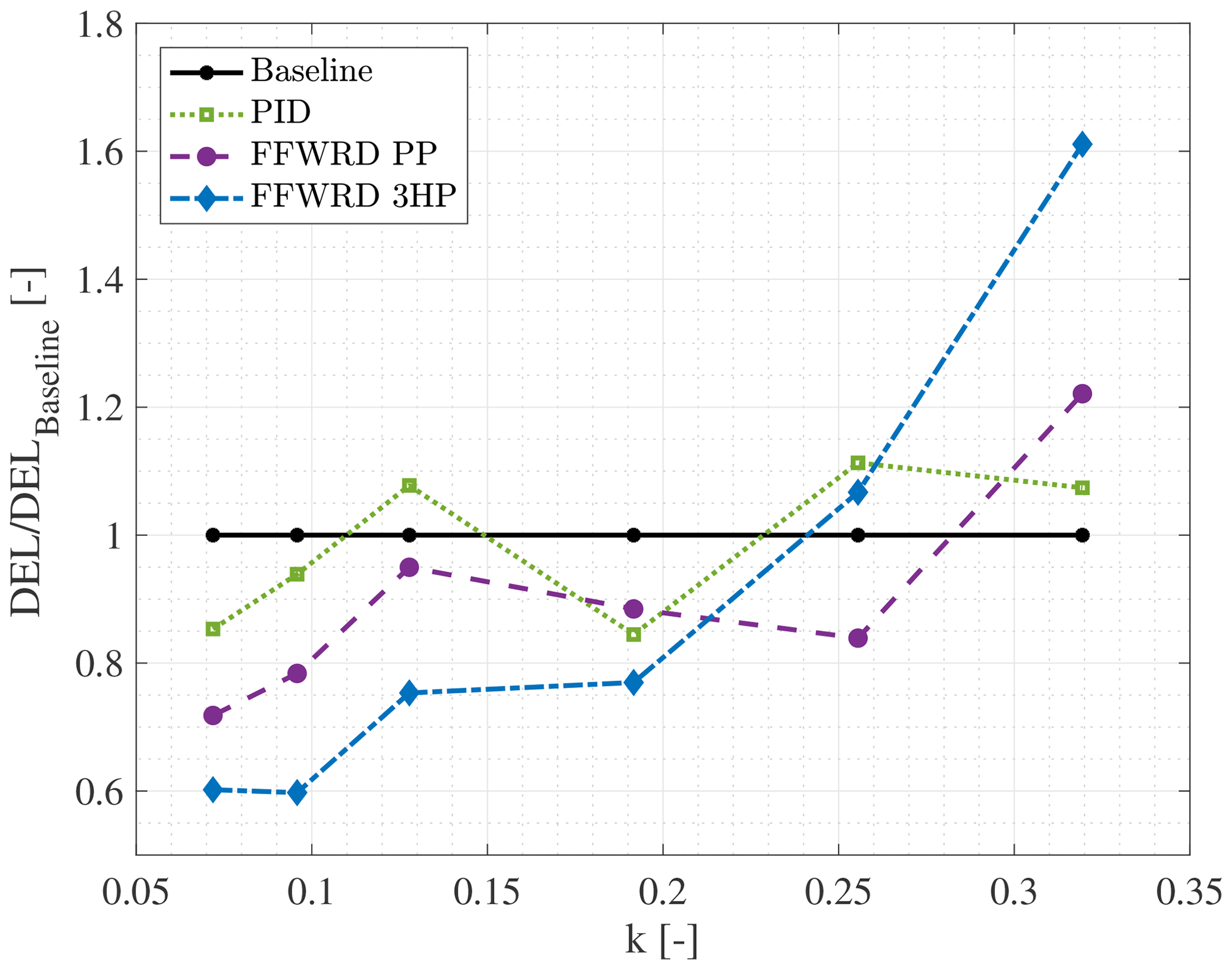
Figure 20Comparison of short-term damage equivalent loads for feedforward and feedback control.
At the reduced frequency of k=0.072, the force-balance-based PID controller is capable of reducing the DEL to 85.33 %. Employing the PP feedforward controller reduces the DEL to 71.8 %, and an even greater reduction is achieved by employing the 3HP feedforward controller to a DEL of 60.2 %. The lower performance of the PID controller is to be expected, as feedback control has to experience a changing load first before it can react to it. Feedforward control is capable of counteracting the changing inflow before it are felt by the wing. Despite the lift estimation based on the three-hole probe having a lower accuracy than the pressure-surface-based estimation (as seen in Fig. 18), the 3HP controller is superior in comparison to the other controllers. This indicates that in this test case the phase lead seen for the three-hole probe lift estimation is more decisive for the success of the controller strategy than the inaccuracies of the lift estimation.
7.2 Inflow disturbance at a reduced frequency of k=0.096 (f=1.5 Hz)
At the reduced frequency of k=0.096 the trends concerning the DELs are generally kept (Fig. 20). However, the success of the feedback control is lowered with a DEL of 93.9 % compared to the baseline. The PP controller performance is also slightly lowered to 78.4 %, whereas the 3HP controller result remains almost constant at 59.8 %. The lower alleviation level of the feedback control and the PP controller can be explained by the increasing challenge at higher frequencies of the inflow disturbance. This affects the 3HP controller less, as the phase lead of the lift estimation increases and the error slightly decreases (see Fig. 18).
7.3 Inflow disturbance at a reduced frequency of k=0.128 (f=2.0 Hz)
At the reduced frequency of k=0.128 the feedback controller fails to reduce the DEL and the PP controller has a very small positive effect on the DEL, resulting in a level of 95.0 %. In contrast, the 3HP controller still reduces the fluctuation loads to a level of 75.3 % even though the load alleviation is not as good as seen for lower frequencies.
In order to understand the lowered performance of the different controller settings, it is worth looking at the (cumulative) power spectral density (CPSD) given in Fig. 21. As seen in this plot, the wing is not only affected by a disturbance at the base frequency of k=0.128, corresponding to f=2 Hz, but also significantly by its first harmonic at a reduced frequency of k=0.256. The CPSD further shows that at the base frequency of f=2 Hz all controllers successfully reduce the fluctuation in comparison to the baseline (see black line in lower plot Fig. 21). In agreement with the previous result at lower frequencies, the 3HP controller is superior to the PP controller and the feedback controller. At the first harmonic (f=4 Hz) the step that each cumulative power spectral density experiences is quite conclusive. The baseline increase in the cumulative power spectral density at this frequency is , whereas the increase seen by the PID controller is , for the PP controller and for the 3HP controller. This demonstrates that the 3HP controller has a comparable contribution to the overall loading as the baseline case at this frequency. On the contrary, the other controller types add significant loading at the first harmonic. Recalling that the calculation of DELs is based on rain-flow counting of cycles and weighting them by the Wöhler function, it is evident that a larger amplitude at the same frequency leads to more damage and hence more damage equivalent loading. As only the increase in loading at the first harmonic (f=4 Hz) for the 3HP controller is close to the baseline case, this controller strategy shows the lowest level of DELs (see blue line Fig. 20). It is expected that a pure harmonic disturbance would have been successfully alleviated by all controller configurations.

Figure 21PSD and CPSD of the lift amplitude for the inflow disturbance with a base frequency of k=0.128.
7.4 Inflow disturbance at a reduced frequency of k=0.192 (f=3.0 Hz)
Figure 20 shows the DELs at the reduced frequency of k=0.192. It can be seen that the difference between the DELs of all studied cases decreases. The PID controller achieves a reduction to 84.5 %, the PP controller achieves a reduction to 88.5 % and the 3HP controller sees a slight increase in comparison to its previous result to a level of 77.0 %.
Furthermore, in order to understand the performance of the different controller settings, it is worth looking at the CPSD, given in Fig. 22. The result seen in terms of CPSD is comparable to the case seen for the test case at k=0.128. In this particular test case, the disturbance at a frequency of f=3 Hz leads to an increase in CPSD for all controller settings. Furthermore, the 3HP controller is the most effective for this frequency, leading to an increase to , which is 38 % of its baseline equivalent. Furthermore, the PP controller reduces the load at this frequency to a level of 57 % and the PID controller results to 76 %. This trend is not seen so clearly for the DELs, Fig. 20, as the first harmonic (f=6 Hz) of the disturbance frequency has to be considered as well. Here, the PID controller experiences the smallest step , whereas the two feedforward controllers see both an increase in and .
In order to understand this effect, it is worth looking at the different phases introduced by the lift estimates (Fig. 18) and by the low-pass filter (Fig. 13). In particular, the latter introduces a phase shift of with an additional phase shift due to the mechanics of the trailing-edge flap of and the phase due to update time , resulting in a phase of . This indicates that all controllers fail to alleviate loads at this frequency for the current mechanical, controller and low-pass filter setup. It is expected that this effect is less severe for the PID controller for multiple reasons: first of all, the frequency of 6Hz is beyond the phase turning point described in Sect. 6.1, where the phase of the lift leads the flap motion due to added mass effects. The latter is seen by the force balance but not by the pressure-based lift estimation methods. Thereby, a phase lead of the balance of is present in comparison to the pressure-based methods. Secondly, as the force balance measurement is also affected by the force of the acceleration of the flap inertia, the change in lift due to flap motion is substantially less in comparison to pressure-based methods. This can be seen at marker A in Fig. 13, where the gain of the lift amplitude is measured to 25 % by the force balance due to a 180∘ phase shift between the aerodynamic lift and the force created by the acceleration of the flap inertia. Hence, the pressure-based methods estimate a substantially larger lift from the flap motion than what is actually measured in the force balance, leading to larger flap deflections and thereby to larger amplitudes at f=6 Hz.

Figure 22Cumulative power spectral density of the lift amplitude at the reduced frequency of k=0.192.
The disturbances with frequencies of k=0.256 and k=0.319, corresponding to frequencies f=4 and f=5 Hz respectively, are given for completeness to show where the controller options fail.
7.5 Inflow disturbance at a reduced frequency of k=0.256 (f=4.0 Hz)
Furthermore, Fig. 20 shows the DELs at a reduced frequency of k=0.256. It can be seen that the PID and the 3HP controllers fail to lower the level of the damage equivalent load, whereas the PP controller achieves a level of 84 % of its baseline equivalent. The corresponding cumulative power spectral density is given in Fig. 23, confirming that the PID and the 3HP controllers already fail to alleviate the applied fluctuating load at k=0.256. Additionally, the PP controller has a slightly higher CPSD level at f=4 Hz as the baseline, indicating that this controller is also not capable of alleviating the introduced load at this frequency.
This result is contradictory in comparison to the load alleviation seen at the first harmonic (f=4 Hz) in the k=0.128 case. This gives rise to the following questions. First, why is the result of the 3HP controller significantly worse? Second, why is the PP controller a lot better than what was seen previously at this frequency?
Concerning the failure of the 3HP controller, the phase lag introduced by the low-pass filter, update time and the flap mechanics, , has to be taken into account, which leads to the poor load alleviation result. Furthermore, it is important to note that the error of the lift estimation of the three-hole probe starts to increase significantly at this frequency, Fig. 18. In particular, the NRMS of the three-hole probe estimate increases to 19.7 %, caused by a significant overestimation of the lift amplitudes as seen in the time series (see Fig. 17, k=0.256). It is expected that for the considered frequency of f=4 Hz this effect is more significant for the k=0.256 case than for the k=0.128 case, as the amplitude of the lift fluctuation is 21.4 % larger ( in comparison to ). This is reflected by an over-proportional increase in the flap motion amplitude of by 70.6 % to .
In order to answer the second question of why the PP controller shows a successful reduction of the DEL to a level of 83.9 % (see Fig. 20), the time series is considered first (see Fig. D4, lower plot). It can be observed that the resulting lift is changed in mean level, but the maximum peak-to-peak level is almost unaltered when comparing the PP controller to the baseline result.
This is reflected in the cumulative power spectral density (see Fig. 23). The step at f=4Hz, corresponding to the reduced frequency of k=0.256, amounts to for the PP controller, which is slightly larger in comparison to the baseline case ().
Hence, the PP controller does not successfully alleviate the loading at f=4Hz.
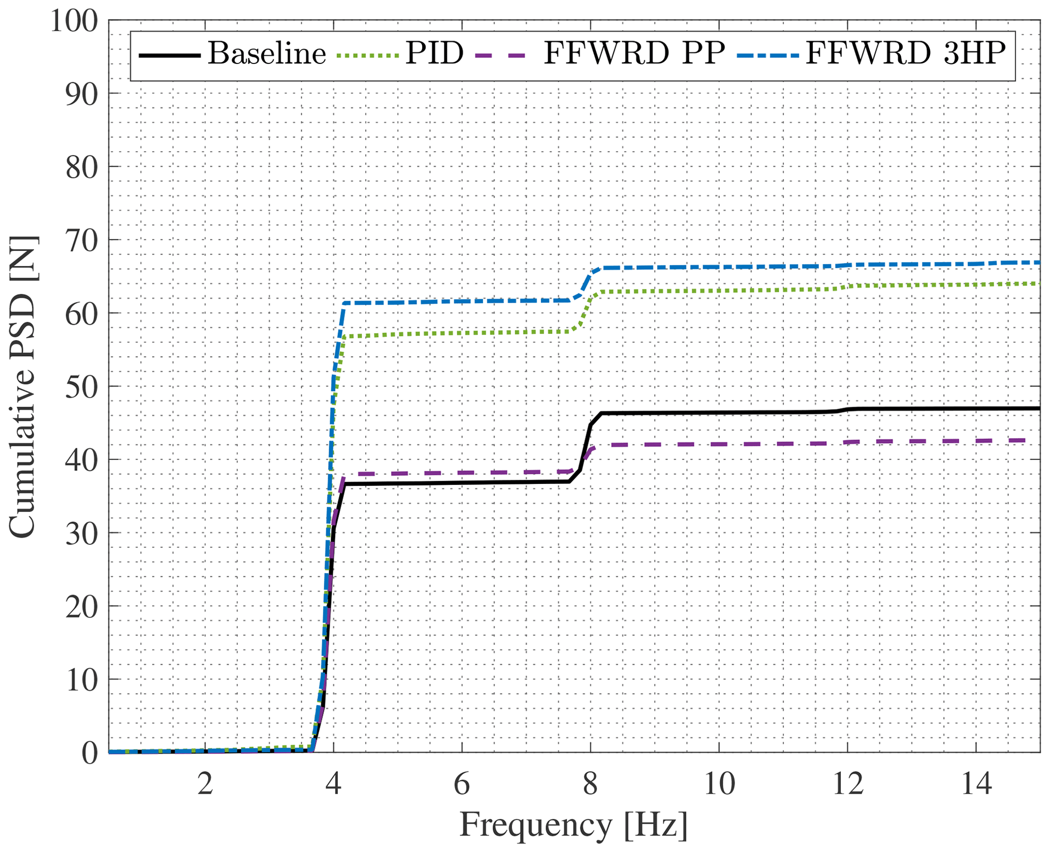
Figure 23Cumulative power spectral density of the lift amplitude at the reduced frequency of k=0.256.
As a sidenote, when the signals are low-pass filtered at f=6 Hz, thus including the disturbance frequency but cutting the first harmonic at f=8 Hz out and then calculating the DELs, the result of the failing PP controller is confirmed. However, when including the first harmonic at f=8 Hz, the DEL is smaller for the PP controller. Therefore, the loading at f=8 Hz has to be considered as well. As seen in Fig. 23, the step at this frequency for the PP controller () is substantially smaller than for the baseline case (). This leads to the apparent lower DEL result seen in Fig. 20 and also to a lower CPSD level for the PP controller (see Fig. 23). It is expected that the lower step in CPSD at f=8 Hz is caused by the configuration of this particular test rig and the employed controller configuration. As seen in Fig. 13, above a frequency of f=7 Hz the lift response due to flap motion is inverted due to the force that is created by the acceleration of the flap inertia. This creates a phase shift for the lift response due to flap motion of . Taking into account the large phase due to low-pass filter, mechanics and update time , these two effect partially cancel each other out, leading to a certain improvement of the 8 Hz disturbance. As these frequencies are out of the scope of this paper, they were not further analyzed.
7.6 Inflow disturbance at a reduced frequency of k=0.319 (f=5.0 Hz)
The final test case is given by an inflow disturbance with a reduced frequency of k=0.319. Figure 20 shows that both feedforward strategies fail to lower the fluctuating load. This can be explained by a significant overestimation of the lift amplitude by the pressure-based lift estimation methods (see Fig. 17, fifth row). This effect cumulates to a NRMS error of the three-hole probe measurement, Fig. 18, of NRMS3HP=46 % and NRMSPP=19 % for the surface pressure method. Additionally, the introduced phase lag of the low-pass filter and the flap mechanics at f=5 Hz amount to , indicating that the flap motion is almost completely in phase with the lift amplitude. This implies that a positive flap-down motion – creating higher lift – is almost in phase with a positive lift amplitude affecting the wing. This can be confirmed when looking at the flap position and lift amplitude given in Fig. D5, third and fourth row.
In this study feedforward control strategies for wind turbine applications to alleviate fluctuating loads on a two-dimensional wing are presented. Three-hole probe or surface pressure port lift estimates served as input for the feedforward control. Within this paper, the lift estimation methods were presented first, and then their application to load control was shown.
In a first step, test cases without inflow disturbance and only flap motion were analyzed. The surface pressure port and the three-hole probe-based estimate agree fairly well with the balance measurements and with the lift that is based on the integration of the complete pressure port set (LFULLPP) up to reduced frequency of k=0.192.
For higher frequencies the amplitude measured by the balance drops due to the mechanical properties of the current setup. The pressure port lift estimate still compares well to the LFULLPP, whereas the three-hole probe estimate overpredicts the gain as unsteady effects are not captured. Furthermore, it is seen that at k=0.318 the phase between flap motion and lift response turns. This effect is not captured by the two presented methods as added mass effects are not incorporated.
Regarding the test cases with inflow disturbance and fixed flap, both methods show good results for the wing exposed to reduced frequency of up to k=0.192. The pressure port lift estimate is generally significantly better than the three-hole probe estimate, as unsteady effects are captured. The latter method overpredicts significantly the lift amplitude. This effect worsens with increasing frequency, as already seen at k=0.255, leading to unacceptable results at k=0.319. Regarding cases where the flap of the wing is additionally actuated, the error of both methods is further increased, whereby the three-hole probe method is more affected. Regarding the phase of both methods, the three-hole probe method is advantageous, especially as the probe head is located upstream of the wing. However, when the flap is active, the phase lead is halved for the three-hole probe method.
The load control results show that the presented pressure-based controllers improve the load alleviation capability of the present trailing-edge flap setup significantly up to a frequency of k=0.192. Even though the three-hole probe-based lift estimate is worse in quality in comparison to the surface pressure port estimate, the phase advantage leads to significant superiority. Moreover, it is expected that in a setup where a pure sinusoidal disturbance can be created, a higher load alleviation potential can be achieved. In the current setup, higher harmonics increase the challenge for the controller setup. Above a frequency of k=0.192 all controller types fail.
The current study presents approaches for lift estimation that may serve as input for load controllers on research or industry-scale turbines. In particular employing surface pressure measurements that do not rely on tubing will be beneficial as they avoid issues such as clogging by insects or dust. Moreover, trailing-edge flaps are a promising device for the alleviation of fatigue and extreme loads of wind turbines.
It is expected that the use of a low-pass filter with increased cut-off frequency or a bandpass filter can further improve the results. Furthermore, creating an unsteady lift estimation method based on the three-hole probe will combine a high-quality lift estimation with an advantageous phase lead. Moreover, incorporating a lookup table for the lift flap slope instead of using a constant value might reduce the estimation error for future applications.
The authors aim at transferring the results to experiments on the Berlin research turbine. It is expected that feedforward control will significantly improve load reduction capabilities of the setup. Furthermore, plans have been made to employ the measurement of the blade root bending moment of the preceding blade as an input to the controller, as this will allow for an additional phase lead, which was shown to be very decisive in this study.
Table B1Coordinates of the pressure taps in reference to the chord and the spanwise position. The according coordinate system is located at the leading edge at the lower spanwise end of the model.

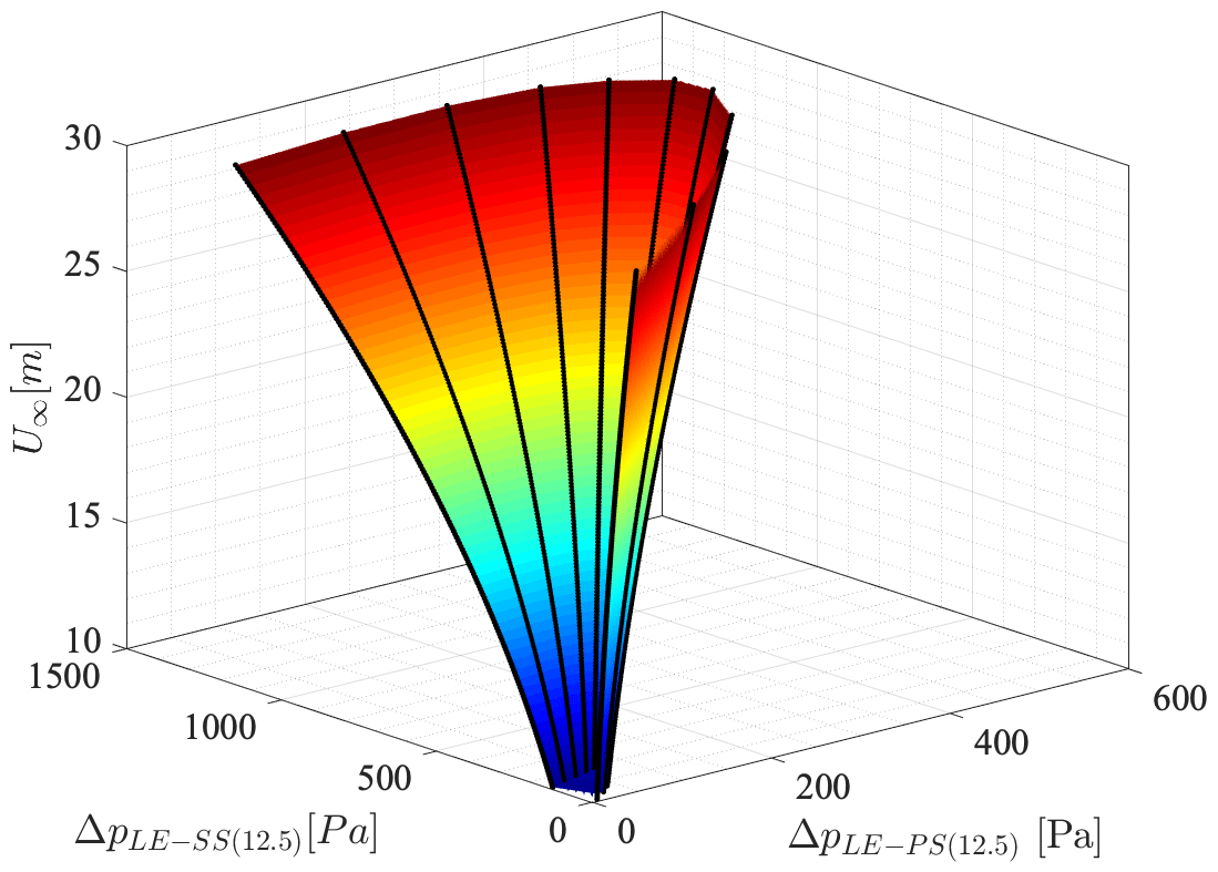
Figure C1Calibration function for estimating the inflow velocity. Example shows the result for a flap angle of .
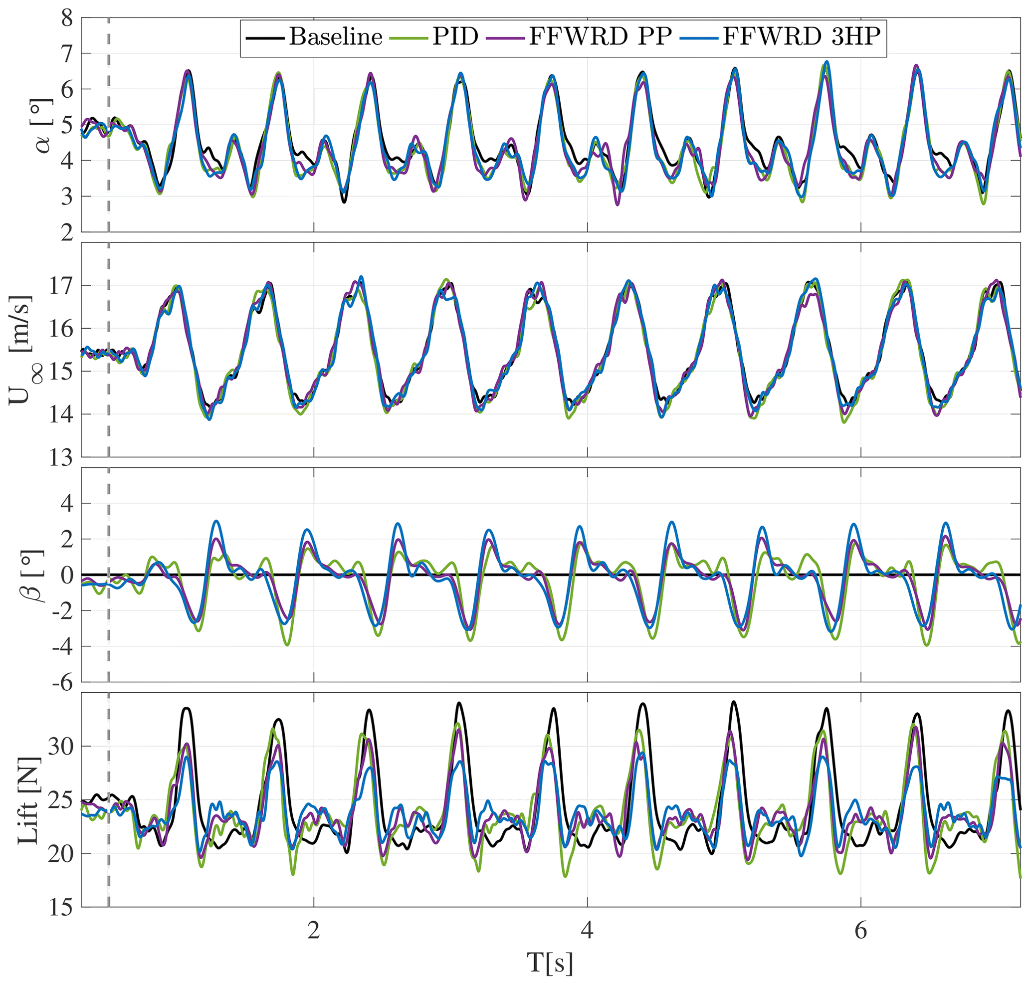
Figure D1Time series of angle of attack and velocity variation, flap motion, and resulting lift amplitude at a reduced frequency of k=0.096.

Figure D2Time series of angle of attack and velocity variation, flap motion, and resulting lift amplitude at a reduced frequency of k=0.128.
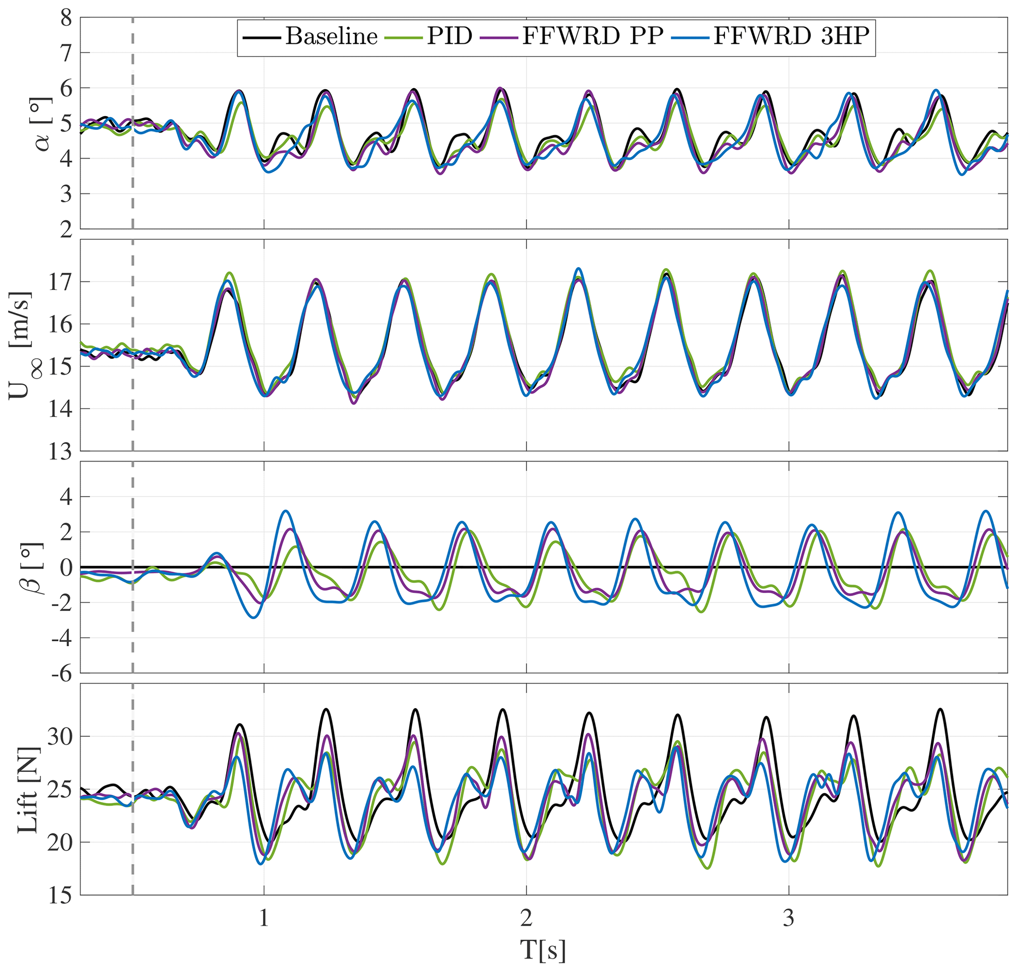
Figure D3Time series of angle of attack and velocity variation, flap motion, and resulting lift amplitude at a reduced frequency of k=0.192.
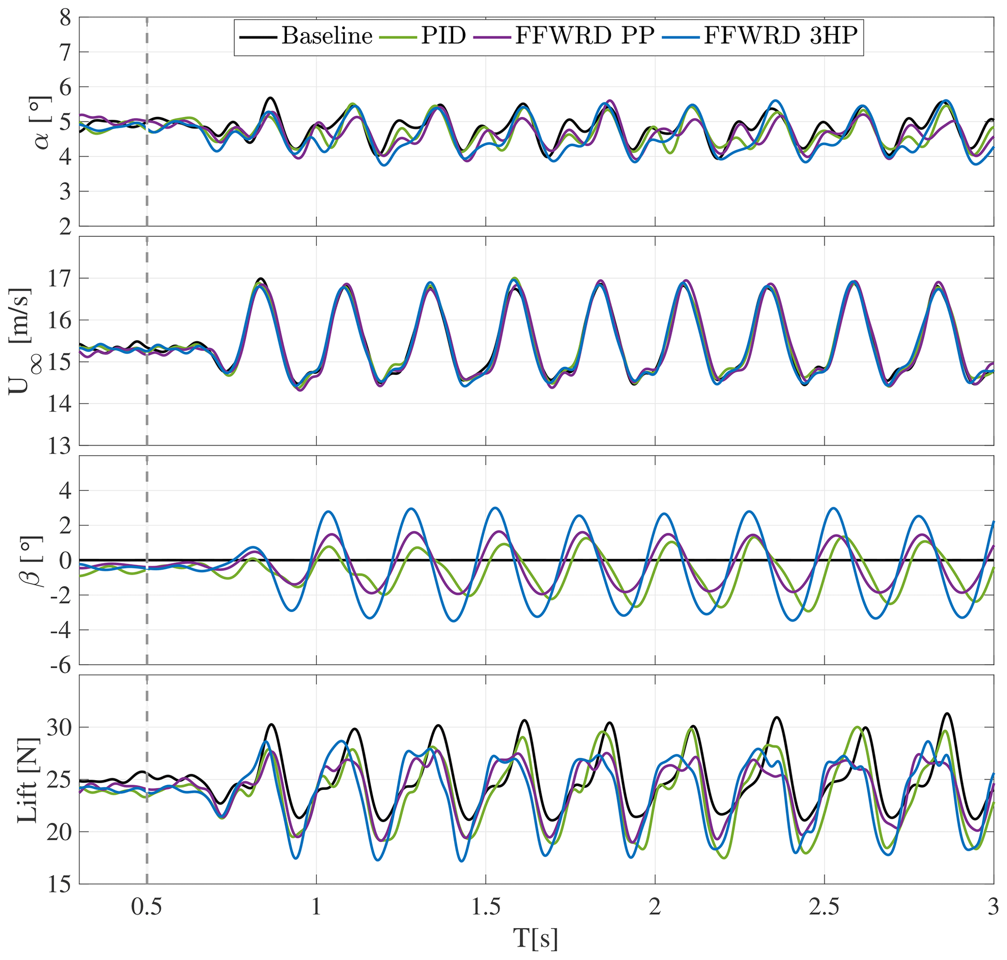
Figure D4Time series of angle of attack and velocity variation, flap motion, and resulting lift amplitude at a reduced frequency of k=0.256.
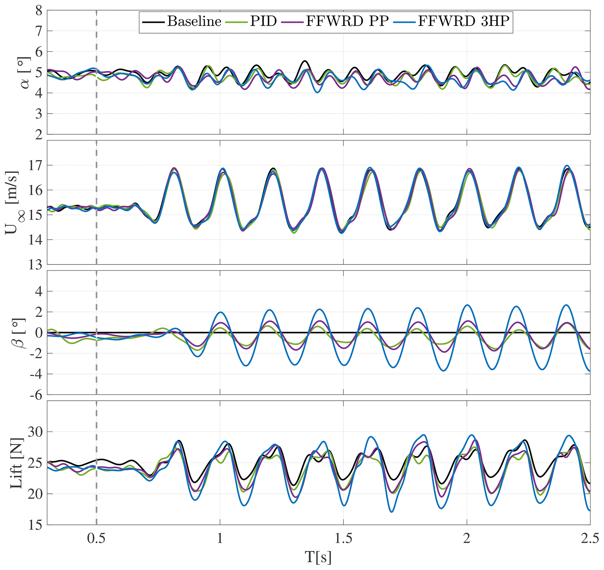
Figure D5Time series of angle of attack and velocity variation, flap motion, and resulting lift amplitude at a reduced frequency of k=0.319.

Figure E1Cumulative power spectral density of the lift amplitude at the reduced frequency of k=0.319.
Table F1Summary of the load alleviation results. ΔCPSDbase[N2] denotes the increase in cumulative spectral density at the base frequency. Accordingly, ΔCPSD1st[N2] corresponds to the increase at the first harmonic. Bold font indicates a load alleviation in comparison to the baseline; italic font corresponds to an increase in loading.
Data can be made available upon request.
SB led the design and construction process of the wing. He also conducted the experiments, programmed the controller, developed the lift estimation methods, post-processed data and wrote this publication. TTBW programmed the active inflow grid and supported the measurements. SPB helped in the analysis and interpretation of the load control results and also in streamlining and proofreading of the manuscript. SK and AS designed the flexible hinge. CM was in charge of the electric wiring and programmed the LabVIEW code, including the communication to the servo motor. MH is the head of the wind tunnel facility that was used. JP, CNN and COP are the project leaders of the related research project. KO is the PhD supervisor of the first author. He was involved in the data analysis and substantially helped to draft the paper.
The authors declare that they have no conflict of interest
This research has been supported by the Deutsche Forschungsgemeinschaft (grant no. DFG PAK 780II).
This open-access publication was funded
by Technische Universität Berlin.
This paper was edited by Mingming Zhang and reviewed by two anonymous referees.
Andersen, P. B., Gaunaa, M., Bak, C., and Buhl, T.: Load Alleviation on Wind Turbine Blades Using Variable Airfoil Geometry, in: European Wind Energy Conference, Athens, Vol. 3, 1880–1887, 2006. a
Arnold, J. I. and Dempster, J. B.: Flight test evaluation of an advanced stability augmentation system for B-52 aircraft, J. Aircraft, 6, 343–348, https://doi.org/10.2514/3.44062, 1969. a
Åström, K. J. and Murray, M. R.: Feedback Systems: An Introduction for Scientists and Engineers, Princeton University Press, ISBN 9780691135762, 2008. a
Bak, C., Gaunaa, M., Andersen, P. B., Buhl, T., Hansen, P., Clemmensen, K., and Moeller, R.: Wind Tunnel Test on Wind Turbine Airfoil with Adaptive Trailing Edge Geometry, in: 45th AIAA Aerospace S, Reno, NV, USA, 8–11 January 2007, AIAA2007-1016, https://doi.org/10.2514/6.2007-1016, 2007. a
Bak, C., Zahle, F., Bitsche, R., and Kim, T.: The DTU 10-MW reference wind turbine, Danish wind power, available at: https://orbit.dtu.dk/en/publications/the-dtu-10-mw-reference-wind-turbine (last access: 28 January 2020), 2013. a
Bartholomay, S., Fruck, W.-L., Pechlivanoglou, G., Nayeri, C. N., and Paschereit, C. O.: Reproducible Inflow Modifications for a Wind Tunnel Mounted Research Hawt, ASME Turbo Expo 2017: Turbomachinery Technical Conference and Exposition, Charlotte, North Carolina, USA, 26–30 June 2017, GT2017-64364, https://doi.org/10.1115/GT2017-64364, 2017. a, b, c, d
Bartholomay, S., Michos, G., Perez-Becker, S., Pechlivanoglou, G., Nayeri, C., Nikolaouk, G., and Paschereit, C. O.: Towards Active Flow Control on a Research Scale Wind Turbine Using PID controlled Trailing Edge Flaps, Wind Energy Symposium, American Institute of Aeronautics and Astronautics, Kissimee, FL, USA, 8–12 January 2018, AIAA, 2018-1245https://doi.org/10.2514/6.2018-1245, 2018. a, b, c, d
Basualdo, S.: Load Alleviation on Wind Turbine Blades Using Variable Airfoil Geometry, Wind Eng., 29, 169–182,https://doi.org/10.1260/0309524054797122, 2005. a
Bergami, L. and Gaunaa, M.: ATEFlap Aerodynamic Model, a dynamic stall model including the effects of trailing edge flap deflection Risø-R-1792(EN), Vol. 1792, DTU Risø, Roskilde, Denmark, 2012. a
Bergami, L., Gaunaa, M., and Heinz, J.: Indicial lift response function: an empirical relation for finite-thickness airfoils, and effects on aeroelastic simulations, Wind Energy, 16, 681–693, https://doi.org/10.1002/we.1516, 2013. a
Bernhammer, L. O., Breuker, R. D., Karpel, M., and van der Veen, G. J.: Aeroelastic Control Using Distributed Floating Flaps Activated by Piezoelectric Tabs, J. Aircraft, 50, 732–740, https://doi.org/10.2514/1.C031859, 2013. a
Buhl, T., Gaunaa, M., and Bak, C.: Potential load reduction using airfoils with variable trailing edge geometry, J. Sol. Energ.-T ASME, 127, 503–516, https://doi.org/10.1115/1.2037094, 2005. a, b
Campagnolo, F., Bottasso, C. L., and Bettini, P.: Design, manufacturing and characterization of aero-elastically scaled wind turbine blades for testing active and passive load alleviation techniques within a ABL wind tunnel, J. Phys. Conf. Ser., 524, 012061, https://doi.org/10.1088/1742-6596/524/1/012061, 2014. a, b
Castaignet, D., Barlas, T., Buhl, T., Poulsen, N. K., Wedel-Heinen, J. J., Olesen, N. A., Bak, C., and Kim, T.: Full-scale test of trailing edge flaps on a Vestas V27 wind turbine: active load reduction and system identification, Wind Energy, 17, 549–564, https://doi.org/10.1002/we.1589, 2014. a
Cooperman, A. and Martinez, M.: Load monitoring for active control of wind turbines, Renew. Sust. Energ. Rev., 41, 189–201, https://doi.org/10.1016/j.rser.2014.08.029, 2015. a, b
Drela, M. and Youngren, H.: XFOIL; Subsonic Airfoil Development System, available at: https://web.mit.edu/drela/Public/web/xfoil/ (last access: 5 May 2019), 2001. a, b
Gaunaa, M.: Unsteady 2D potential-flow forces on a thin variable geometry airfoil undergoing arbitrary motion, Tech. rep., Risø National Laboratory, 2006. a, b
Gaunaa, M. and Andersen, P. B.: Load reduction using pressure difference on airfoil for control of trailing edge flaps, in: EWEC 2009 Proceedings online, EWEC, 2009 European Wind Energy Conference and Exhibition, Marseille, France, 2009. a, b, c, d, e, f, g, h, i
Hayman, G. J.: MLife Theory Manual for Version 1.00, National Renewable Energy Labaratory, Golden, CO, USA, 2012. a
Heinze, S. and Karpel, M.: Analysis and Wind Tunnel Testing of a Piezoelectric Tab for Aeroelastic Control Applications, J. Aircraft, 43, 1799–1804, https://doi.org/10.2514/1.20060, 2006. a
Iribas, M., Hansen, M., Mizaei, M., Tibaldi, C., Natarajan, A., and Bossanyi, E.: INNWIND Deliverable Report D1.42 Methodology for Feed-Forward Control Strategies using Nacelle or Blade Based Sensors and Distributed Control (Vol. Deliverabl), available at: http://www.innwind.eu/publications/deliverable-reports (last access: 29 January 2020), 2015. a, b
Klein, A. C., Bartholomay, S., Marten, D., Lutz, T., Pechlivanoglou, G., Nayeri, C. N., Paschereit, C. O., and Krämer, E.: About the suitability of different numerical methods to reproduce model wind turbine measurements in a wind tunnel with a high blockage ratio, Wind Energ. Sci., 3, 439–460, https://doi.org/10.5194/wes-3-439-2018, 2018. a, b, c, d, e
Komusanac, I., Brindley, G., and Fraile, D.: Wind energy in Europe in 2019, available at: https://windeurope.org/wp-content/uploads/files/about-wind/statistics/WindEurope-Annual-Statistics-2019.pdf (last access: 5 April 2019), 2020. a
Leminos, A. Z. and Smith, A. F.: An Analysgtical Evaluation of the Controllable Twist Rotor Performance and Dynamic Behavior, Tech. rep., U.S. Army Air Mobility Research and Development Laboratory, Fort Eustis, VA, USA, 1972. a
Marrant, B. A. H. and van Holten, T.: Comparison of Smart Rotor Blade Concepts for Large Offshore Wind Turbines, in: Offshore Wind Energy Other Renewable Energies Med. Euro. Seas, Civitavecchia, Italy, 2006. a, b
Motta, V., Guardone, A., and Quaranta, G.: Influence of airfoil thickness on unsteady aerodynamic loads on pitching airfoils, J. Fluid Mech., 774, 460–487, https://doi.org/10.1017/jfm.2015.280, 2015. a
Navalkar, S. T., Bernhammer, L. O., Sodja, J., Slinkman, C. J., Van Wingerden, J. W., and Van Kuik, G. A.: Aeroelastic Design and LPV Modelling of an Experimental Wind Turbine Blade equipped with Free-floating Flaps, J. Phys. Con. Ser., 753, 042010, https://doi.org/10.1088/1742-6596/753/4/042010, 2016. a
NREL: (MLife), NWTC Information Portal, available at: https://nwtc.nrel.gov/MLife (last access: 1 April 2019), 2015. a
Pechlivanoglou, G., Nayeri, C. N., and Paschereit, C. O.: Performance Optimization of Wind Turbine Rotors With Active Flow Control, ASME 2011 Turbo Expo: Turbine Technical Conference and Exposition 6–10 June 2011, Vancouver, Canada, 763–775, https://doi.org/10.1115/GT2011-45493, 2011. a
Petersen, M. M., Larsen, T. J., Larsen, G. C., Madsen, H. A., Larsen, G., and Troldborg, N.: Turbulent wind field characterization and re-generation based on pitot tube measurements mounted on a wind turbine, 33rd Wind Energy Symposium, Kissimmee, USA, 5–9 January 2015, AIAA 2015-1467 https://doi.org/10.2514/6.2015-1467, 2015. a, b
Pedersen, M. M., Larsen, T. J., Madsen, H. Aa., and Larsen, G. Chr.: Using wind speed from a blade-mounted flow sensor for power and load assessment on modern wind turbines, Wind Energ. Sci., 2, 547–567, https://doi.org/10.5194/wes-2-547-2017, 2017. a, b
Plumley, C.: The Smart Rotor Wind Turbine, PhD thesis, University of Strathcycle, Glascow, UK, 2015. a, b
Sandford, M. C., Abel, I., and Gray, D. L.: Development and demonstration of a flutter-suppression system using active controls, Tech. Rep. NASA TR R-450, NASA, 1975. a
Sedano, C., Berger, F., Rahimi, H., Lopez Mejia, O., Kühn, M., and Stoevesandt, B.: CFD Validation of a Model Wind Turbine by Means of Improved and Delayed Detached Eddy Simulation in OpenFOAM, Energies, 12, 1306, https://doi.org/10.3390/en12071306, 2019. a
Shen, J. and Chopra, I.: Swashplateless Helicopter Rotor with Trailing-Edge Flaps, J. Aircraft, 41, 208–214, https://doi.org/10.2514/1.9279, 2004. a
Shipley, D., Miller, M., Robinson, M., and Luttges, M.: Techniques for the Determination of Local Dynamic Pressure and Angle of Attack on a Horizontal Axis Wind Turbine, Tech. Rep. NREL/TP-442-7393, National Renewable Energy Labaratory, USA, 1995. a
Thornburgh, R. P., Kreshock, A. R., Wilbur, M. L., Sekula, M. K., and Shen, J.: Continuous Trailing-Edge Flaps for Primary Flight Control of a Helicopter Main Rotor, Tech. rep., Montreal; Canada, available at: https://ntrs.nasa.gov/search.jsp?R=20140006537 (last access: 2 April 2019), 2014. a
Troldborg, N.: Computational Study of the Risø-B1-18 Airfoil with a Hinged Flap Providing Variable Trailing Edge Geometry, Wind Eng., 29, 89–113, https://doi.org/10.1260/0309524054797159. 2005. a
Velte, C., Mikkelsen, R. F., Sørensen, J. N., Kaloyanov, T., and Gaunaa, M.: Closed loop control of a flap exposed to harmonic aerodynamic actuation science of making torque from wind, Proceedings of The Science of Making Torque From Wind, 2012. a, b, c, d, e, f
Wester, T. T. B., Bartholomay, S., Traphan, D., Hölling, M., Peinke, J., and Gülker, G.: Using high speed PIV measurements and POD to solve the mystery of dynamic stall, 19th International Symposium on the Application of Laser and Imaging Techniques to Fluid Mechanics, Lisbon, Portugal, 16–19 July 2018, 2018. a
- Abstract
- Introduction
- Experimental setup
- Lift estimation methods
- Controller design
- Metrics for comparison of load control devices
- Results of the lift estimation methods
- Results of the load control
- Summary and conclusion
- Appendix A: Nomenclature
- Appendix B: Coordinates of the surface pressure ports
- Appendix C: Lookup table for the estimation of the inflow velocity
- Appendix D: Time series
- Appendix E: Power spectral density
- Appendix F: Summary of the load alleviation results
- Data availability
- Author contributions
- Competing interests
- Financial support
- Review statement
- References