Computational fluid dynamics studies on wind turbine interactions with the turbulent local flow field influenced by complex topography and thermal stratification

This paper shows the results of computational fluid dynamics (CFD) studies of turbulent flow fields and their effects on a wind turbine in complex terrain. As part of the WINSENT project, a research test site comprising four meteorological masts and two research wind turbines is currently being constructed in the Swabian Alps in southern Germany. This work is an essential part of the research of the southern German wind energy research cluster WindForS. The test site in complex terrain is characterised by a densely forested escarpment and a flat plateau downstream of the slope. The met masts and wind turbines are built on this plateau.

In the first part, high-resolution delayed detached eddy simulations are performed to separately investigate the effects of the forested escarpment and of thermal stratification on the flow field and accordingly on the wind turbine. In the second part, both these effects are included for a real observed case in March 2021. There, unstable conditions prevailed and the forest showed low leaf area densities due to the winter conditions.

It is shown that atmospheric turbulence, forests, orographies, and thermal stratification must be considered when assessing the impact on wind turbines in complex terrain. All of these effects influence the flow field both at the turbine position and in its wake. The wind speed at the test site is accelerated by up to 60 %, which could affect the annual energy production significantly. But otherwise turbulent structures of the forest wake cross the rotor plane temporarily and thereby affect the turbine inflow. Moreover, convective conditions and upward flows caused by the orography have an impact on the turbine's power output as inclined flows result in asymmetric torque distributions. The wind turbine wake and the forest wake mix further downstream, resulting in a faster decay of the turbine wake than in neutral conditions or without forest. The paper also describes how the turbulent flow in the wake changes in the presence of thermal stratification, which is evident in order to be able to numerically represent the flow-physical changes in the diurnal cycle well.

1 Introduction

1.1 Numerical modelling of atmospheric turbulence in complex terrain

In terms of wind turbine site assessment, complex topographies remain a major challenge. Because some research questions on this topic are still unanswered, the importance of these investigations has been recognised for many years. Wegley et al. (1980) evaluated wind fields in complex terrain and demonstrated that orography-related speed-up of the wind can be conducive to the beneficial use of wind energy. Using Reynolds-averaged Navier–Stokes (RANS) methods, the time-averaged speed-up, which means the acceleration downstream of the escarpment compared to the wind speed in the valley, and the mean flow inclination can in general be predicted well (Brodeur and Masson, 2008). But RANS methods encounter difficulties over complex terrain and also in the case of strongly changing topographic and thermal conditions of the local flow field, which cannot be adequately modelled, since unsteady effects cannot be captured correctly due to the averaging of the flow variables by RANS methods. Barber et al. (2022), for example, showed that there are still large uncertainties in numerical methods, resulting in significant inaccuracies in the prediction of annual energy production (AEP).

With the assistance of filtering, it is possible to numerically resolve large-scale (grid-scale) eddies by means of large eddy simulations (LESs). Thus, large-scale eddies can be resolved numerically, whereas small-scale (sub-grid-scale) flow fluctuations are still modelled as with RANS methods (Ross, 2008). However, LES methods also require immensely fine grid resolutions in the vicinity of the wall, which is why they are not feasible for many high-fidelity applications and the computational power of supercomputers. One solution lies in hybrid RANS simulations and LESs (Weihing et al., 2016). Through combinations of RANS and LES methods, it is possible to calculate certain areas of special interest using LES methods, while the other areas are modelled in RANS mode. Hence, with hybrid RANS and large eddy simulation (LES) methods, even small vortices detached from the ground are resolved, increasing the accuracy of the simulations of the turbulent flow field in complex terrain (Bechmann and Sørensen, 2010). These hybrid RANS/LES methods are usually required for high-fidelity calculations, because topographic effects (such as forests) and atmospheric stability have a significant influence on the turbulent flow field. Although it is also possible to consider these effects very well with RANS methods (Sogachev et al., 2012), hybrid methods or LES methods usually produce significantly better predictions (Sørensen and Schreck, 2014). The hybrid method of the so-called delayed detached eddy simulations (DDESs) is adequate for detailed wind turbine simulations, without increasing the computational costs enormously, as would be the case with LES methods and the required fine resolution of the boundary layer (Weihing et al., 2018).

Forests in complex topographies were analysed in a large-scale numerical LES study by Belcher et al. (2012). They noted that forested hills have a more significant impact on the flow situation compared to forest flows in flat terrain. Further, they explained that thermal stratification also has a strong influence on the resulting flow field. Belcher et al. (2012) concluded that forested orographies downstream of an escarpment are more prone to flow separation than orographies without forest cover. Ivanell et al. (2018) conducted a numerical study to compare different simulation methods to experimental data in forested complex terrain and to evaluate their suitability for such conditions. As a result of their study, Desmond et al. (2017) found that thermal stratification also impacts the wake of forests and that turbulent kinetic energy (TKE) changes fundamentally with thermal stability. In a quantitative observational study these effects were also confirmed by Kelly et al. (2014), who investigated shear and turbulence statistics under a wide range of topographic and thermal conditions. Dupont and Patton (2012) also studied in detail the influences of forests and thermal stability on micrometeorology as part of the Canopy Horizontal Array Turbulence Study (CHATS). Inferences were also made about the evolution of turbulence elements interacting with forests under different conditions. Accordingly, it was shown that the turbulent structures differ significantly under different foliage densities and thermal conditions. The importance of considering all these topographic and meteorological phenomena in complex terrain has been confirmed by Finnigan et al. (2020), who have analysed the research and developments in this field over the last decades.

1.2 Influence of topographic and thermal effects on wind turbines

Topographic and thermal effects also have a major influence on wind turbines regarding loads, power, and wake development. Murphy et al. (2020) showed that the orography- and thermal-stability-related shear of the wind profile leads to a discrepancy of up to 5 % in power generation compared to neutral conditions. Thus, to predict the wind turbine power and loads as accurately as possible, thermal stability should be well captured by measurements and simulations. Radünz et al. (2021) have identified the influence of local orographic effects and thermal stability on wind turbine wakes. It becomes apparent that these affect the performance of wind turbines or complete wind farms. Barthelmie et al. (2018) conducted a study to investigate wind turbine wakes in Perdigão in mountainous terrain and discovered that they strongly depend on topography and stability. Thermal stratifications have led to fundamental differences in wake trajectory measurements. Wakes follow the orography more for stable conditions and less for unstable or neutral conditions. For convective conditions, the wake spreads upward. The fact that thermal stability has a significant effect on the wake was also emphasised in the study by Abkar et al. (2016).

1.3 The WindForS test site and preview on the studies

The WindForS project WINSENT attempts to overcome the challenges to predict the effects of flows over complex terrains on wind turbines more accurately by establishing a test site on the Swabian Alps in southern Germany. Four meteorological (met) masts and two research wind turbines are under construction. Thus, a variety of studies can be conducted experimentally and numerically. The test field has already been analysed in other studies within the framework of this project. Using unsteady Reynolds-averaged Navier–Stokes methods, El Bahlouli et al. (2020) and Berge et al. (2021) compared two selected days to unmanned aerial system (UAS) measurements. Barber et al. (2022) also investigated this terrain numerically with regard to AEP and compared the results with measured data.

This paper deals with spatially and temporal highly resolved delayed detached eddy simulations (DDESs) of the flow field at the test site and consequently on the wind turbine. In this work, new findings are presented that expand on previous studies of Schulz et al. (2016) and provide additional insights into the flow there and the wind turbine loads and wake.

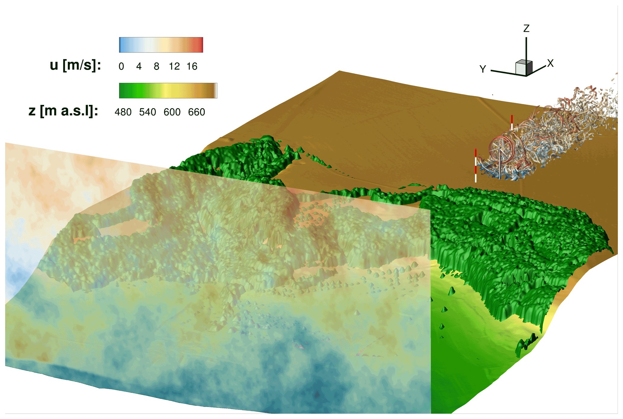
Figure 1 Overview of the numerical flow situations in the test field. In addition to the orography and the turbulent inflow plane, the wind turbine and its interaction with the flow field were also highlighted by λ₂ vortex structures.

Figure 1 shows the entire wind energy test field. Besides the forested orography, the plot also depicts the turbulent inflow plane. The fully meshed wind turbine has been incorporated in its designated position. This means that the wind turbine was positioned in the numerical domain exactly at the position where the real turbine is currently under construction in the test site. Further, vortex structures show the strong interactions of the ambient turbulence and the forest wake with the wind turbine wake. The visualisation of the vortices was performed by the λ₂ criterion, which can be used to determine vortices in a 3 D flow field. The two already existing met masts at the test site are marked. Figure 1 therefore gives a general overview of the analyses in this paper, which include the definition of the inflow turbulence, the propagation of the flow over the forested escarpment, the power and wake analysis of the wind turbine, and the comparison with met mast data. The set-up that serves as a basis for these numerical simulations is explained in the following chapter. The results chapters are divided into two parts to enhance understanding of the emerging effects. The first part will explain the general effects on the flow field to simplify the interpretation of the effects that occur. This includes the characteristics of the orography, the local forest, and thermal stratification. The investigations will show the influence these different aspects have on the flow field. Subsequently, the effects will be applied separately to the wind turbine. The second part will then combine all effects based on real conditions of 10 March 2021. Considering all phenomena explained before, the flow field is then simulated, and the behaviour on the wind turbine performance and its wake will be analysed. The simulations are validated with experimental data from one meteorological (met) mast as the measuring sensors of the second met mast were only available to a limited extent during the observation period.

2 Set-up

In the following, the numerical set-up for the performed simulations in this work will be presented.

2.1 Terrain site and mesh

Figure 2 Background mesh and integration of the fully meshed wind turbine into the area; the mesh has been coarsened 8-fold for presentation reasons. Panel (a) shows the geometric dimensions of the computational domain and the resolution of the hanging grid nodes transverse to the flow direction. Panel (b) shows the resolution of the mesh in the inflow and in the wake of the turbine. A refinement grid around the turbine is also highlighted. Panel (c) shows a surface of the fully resolved turbine and the distances to the two met masts.

Figure 2 shows the geometric dimensions and spatial resolutions of the background mesh. Additionally, the wind turbine is depicted within the background mesh. The domain dimensions are $\mathrm{2400}\times \mathrm{7000}\times \mathrm{2500}$ m in x, y, and z directions. To avoid any perturbations arising from the interaction between the topography and the lateral periodic boundary conditions, a large extension in the y direction was introduced. This procedure serves to avoid numerically induced pressure disturbances that can arise at the lateral boundary conditions if different topologies of the ground are present at these positions. The height of the domain was extracted in the z direction up to 2500 m, since the atmospheric boundary layer can extend higher than 1000 m during summer months. This grid will therefore be equally valid for simulations of a wide range of thermal conditions. To realise these dimensions with also high resolutions in the relevant areas of the test site, the outer cells in the y direction as well as in the z direction were coarsened via hanging grid nodes. Hanging grid node transitions mean that blocks of the mesh with different resolutions are adjacent to each other and that a resolution jump occurs at the border between them. The transition is realised with the help of auxiliary cells. These auxiliary cells are also called dummy layers. The values of the adjacent block are transferred into these cells at the beginning of each Runge–Kutta cycle and serve as the calculation basis for the adjacent physical cells. The relevant areas at the turbine and the met masts were discretised with a resolution of 1 m. This area is 200 m (≈4D) wide in order to simulate the areas of influence of the wind turbines sufficiently with this high resolution. In addition, a wide area of more than 700 m, where the wind turbine is placed in the middle, was meshed with 2 m resolution to still be able to sufficiently resolve the flow physics of large parts of the test site. In the lateral and vertical directions the structured mesh is then quickly coarsened to 4, then to 8, and finally to 16 m to save cells and consequently computational costs. The intermediate areas with 4 and 8 m resolutions are each only about 25 cells wide and are intended to ensure that the transition to 16 m resolution in the outer areas is not too abrupt. As the lower-left plot shows, the highly resolved (1 m) area extends through the entire domain with constant resolution in the x direction to avoid numerical dissipation. The forest mesh is also illustrated within the grid in this section, which can be seen in the bottom area at the escarpment. The application of thermal stability implies additional requirements for the mesh. Unstable stratification requires a very wide and high domain because of the large height of the atmospheric boundary layer and the large length scales, whereas the simulation of stable stratification requires a finer resolution to resolve the small eddies without losing much turbulent information through numerical dissipation. Considering these requirements, without untenably increasing the computational costs, requires a careful choice of the background mesh. The outer region of the mesh is coarsened by hanging grid nodes as described previously. The viscous sublayer at the bottom surface is fully resolved with $z^{+}\approx \mathrm{1}$ ($z^{+}=\frac{z{u}_{*}}{\mathit{\nu }}$). This value is important to determine the position of the wall-nearest grid cell to ensure a good prediction of the wall-bounded turbulent flows. Accordingly, z⁺ is calculated from the wall distance z, the friction velocity u_*, and the kinematic viscosity ν.

To integrate the wind turbine into the field, as shown in the lower-left plot, an additional mesh refinement in the turbine's area was implemented with resolutions of 0.25 m. The wind turbine is fully resolved, which means that the boundary layers of the wind turbine structures (tower, blades, hub, nacelle) are fully meshed with $z^{+}\approx \mathrm{1}$ and $y^{+}\approx \mathrm{1}$.

The coordinate system is an inertial right-hand system that was arranged with x=0 m at the turbine position. For detailed wind turbine evaluations, we used another coordinate system. The origin of this coordinate system is located at hub position of the turbine ($x_{R\mathrm{0}},y_{R\mathrm{0}},z_{R\mathrm{0}}$), which simplifies the interpretation of the results for these studies.

2.2 Numerical set-up

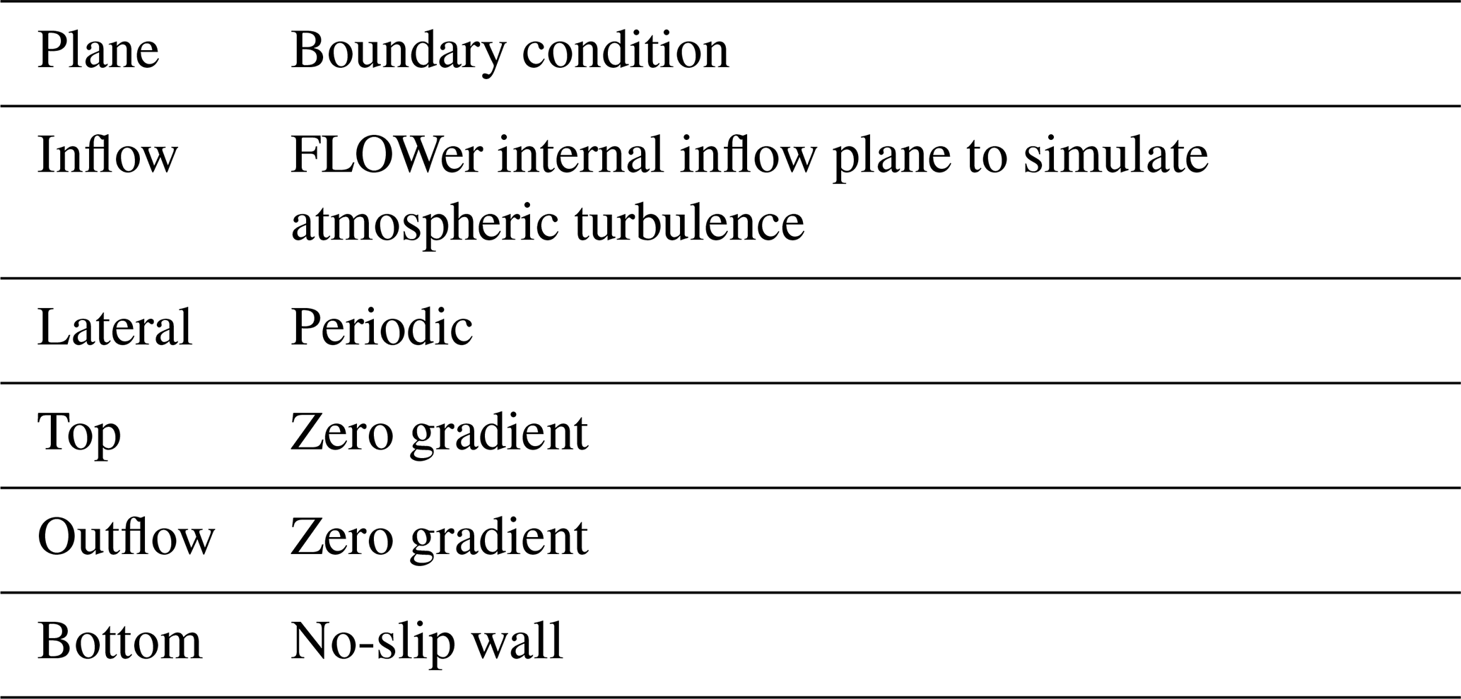
The compressible and block-structured finite volume flow solver FLOWer was used for the simulations. FLOWer was originally developed by the German Aerospace Center, DLR (Kroll et al., 2000). Since then, the code has been extended and improved at the authors' institute for highly resolved simulations of wind turbines. Regarding the boundary conditions, at the inflow a FLOWer internal boundary condition was chosen that allows the inflow of user-defined turbulence fields or turbulence fields extracted from simulations or measurements. These are transient 2 D turbulence fields, which were fed into the computational domain in both of these approaches. Thus, 3 D turbulent fields could be simulated through the propagation of these transient 2 D fields. At the ground a friction no-slip wall with the setting of a wall temperature was used. The lateral boundary conditions were chosen to be periodic. A zero-gradient condition was set at the top boundary and at the outlet. This allowed inflow and outflow across the boundaries and behaves robustly regarding pressure gradients, which is important in turbulent flows and especially for thermal stratification. This boundary condition also suppresses possible reflections of disturbances at the numerical boundaries, which can arise from the standard far-field condition of setting default values at the edges. Table 1 summarises the used boundary conditions.

Table 1 Applied boundary conditions.

Regarding the numerical methods, a second-order Jameson–Schmidt–Turkel scheme (Jameson, 1991) was used to calculate the fluxes in the lowest 10 m near the ground, because of the high aspect ratios caused by small cells and the orography. The rest of the domain was realised with a fifth-order weighted essentially non-oscillatory (WENO) scheme (Schäferlein et al., 2013) for a better preservation of turbulence.

The turbulence model used in the RANS region was the shear-stress-transport (SST) model from Menter (1994). Bangga et al. (2017) obtained the numerically most stable results for FLOWer with this turbulence model in DDES wind turbine simulations, which fit the measured data best, justifying its selection. It is also the most used model in the wind energy and helicopter aerodynamics working groups at the authors' institute. By replacing the turbulent length scale L_RANS outside the boundary layer with the LES filter width, the turbulence model behaves like a Smagorinsky sub-grid-scale model (Weihing et al., 2018). In most areas of the domain the numerical dissipation still overwhelms the physical one introduced by the sub-grid-scale (SGS) model because the fifth-order WENO scheme already introduces numerical dissipation at high wave numbers due to the used Riemann solver (Weihing, 2020). Thereby, it generates eddy viscosity as a function of the strain rate and the filter size. An implicit dual-time stepping is applied for time integration with 100 inner iterations for each time step. This set-up is valid for all simulations of this study. The Courant–Friedrichs–Lewy (CFL) number in the innermost domain was set to 0.4 for the simulations without a wind turbine. Since the characteristics of the wind speed in the lower atmosphere can generally be described by sheared velocity profiles, whereby the wind speed increases above the altitude, the hub height was used as a reference position to determine the CFL number in these studies. After incorporating the wind turbine into the domain, the time step was reduced to adapt it to a rotor azimuth movement of 2^∘, which was needed for detailed aerodynamic evaluations of the turbine. This resulted in a CFL number of 0.2. In order to achieve high accuracy of the results, all studies in this paper were conducted with DDESs. Using this method, a shielding function prevents the attached boundary layer from switching into the LES mode and generating grid-induced separation. The area of the LES region and the region modelled with unsteady Reynolds-averaged Navier–Stokes (URANS) were examined in a preliminary study. For this purpose, the resolved areas of turbulence kinetic energy k_res were compared quantitatively with the total TKE ($k_{\mathrm{tot}}=k_{\mathrm{res}}+k_{\mathrm{mod}}$) for each cell in the whole domain to identify which areas are modelled by URANS and which are resolved by LES. The ratio $\frac{k\mathrm{res}}{k\mathrm{tot}}$ shows to what extent turbulence in certain areas is resolved. This preliminary study revealed that cells within approximately 0.5 m of the ground are not resolved but modelled by URANS. The entire rest of the background mesh is simulated by LES. This preliminary study is valid for all simulations shown in this paper.

2.3 Set-up for the comparisons with measurements

The lower-right plot of Fig. 2 shows the surface structures of the fully meshed wind turbine incorporated into the background mesh with the chimera technique of Benek et al. (1986). With the chimera method, movements/rotations of structures, in this case of the rotor, can be realised through overlapping grids. For the mesh of the rigid turbine, we refer to Guma et al. (2018) and Guma et al. (2021). Just as done for the ground of the terrain, no-slip wall boundary conditions were introduced for the surfaces of the turbine. The two met masts of the test field have also been visualised in this plot to reveal a spatial impression of the test field. The first one served as a validation and comparison basis for this work. The wind turbine is about 135 m downstream of the first and about 135 m upstream of the second met mast as can be seen in Figs. 1 and 2. The two wind turbines and the other two met masts are still under construction and can therefore not serve as validation in this work. With the numerical simulations of the wind turbine, however, far-reaching insights can already be gained through this study.

Table 2 Relevant equipment of the met masts.

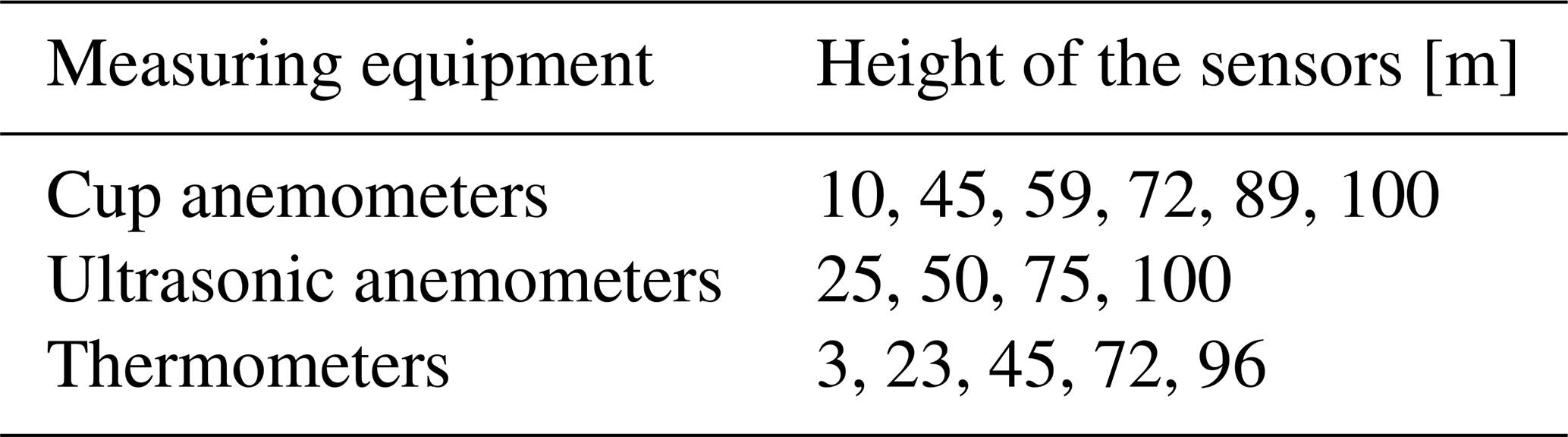
Table 2 reveals the met mast equipment used for this work as a validation basis. The met masts serve for comparisons with numerical results and to extract turbulence characteristics to generate synthetic turbulence at the inflow. Cup anemometers, ultrasonic anemometers, and thermometers are primarily used for these studies. The cup anemometers had a accuracy of 1 %, and the ultrasonic anemometers had an accuracy of 1.5 % (Barber et al., 2022). Both met masts are equipped equivalently and have been installed downstream of each other in the mean flow direction. The met masts and the wind turbine are located directly downstream of each other with negligible lateral offset. The orographic conditions on the plateau are very flat with only small height differences between the met masts and the wind turbine.

2.4 Forest set-up

As seen in Fig. 1, large parts of the test site, especially the escarpment, are covered by a dense forest. To be able to model vegetation in the simulation, adaptations in the FLOWer code are required, which were implemented in previous works (Letzgus et al., 2018). This vegetation model is used in this way in this work. The applied method of Letzgus et al. (2018) is based on the model of Shaw and Schumann (1992) for the implementation of leaf area density profiles vs. tree height.

$$\begin{array}{}\text{(1)}& F_F=\mathit{\rho }\cdot c_{\mathrm{d}}\cdot a\left(z\right)\cdot \left|u\right|{\stackrel{\mathrm{̃}}{u}}_i\end{array}$$

For this purpose, as described by Eq. (1), a force term was added to the momentum equations to apply forest modelling. Besides the local velocities of the respective spatial direction, the force term also contains an empirical drag coefficient c_d, which is usually given as 0.15 in the literature, and the height-dependent leaf area density (LAD) denoted by a(z). With an appropriate choice from measured or literature data, this parameter can model the drag that the vegetation exerts on the flow field.

For the implementation of the forest, an additional grid structure is embedded into the background grid using the chimera technique in analogy to Letzgus et al. (2018) and Letzgus et al. (2020). In this way, the forest can be accurately defined numerically as a porous medium. Additionally, not only homogeneous forests with constant values of leaf area index (LAI) and a(z) can be modelled, as is typical in the literature, but variable leaf area densities and tree heights can be modelled in each spatial direction. This strongly increases the accuracy of the replication of the forest shape in the simulations. It is implemented by adding a force term to each cell of the forest structure depending on the foliage density and tree height. Variable leaf area densities can thus be realised in any spatial direction.

Figure 3 LAD of forests and their modelling in CFD.

The leaf area densities of two exemplary vegetations and the implementation of forests into the computational fluid dynamics (CFD) domain are illustrated in Fig. 3. Since the leaf area densities of deciduous forests and coniferous forests are different, the upper plot shows two curves for different vegetations. The curve with LAI = 2 m² m⁻² shows a typical LAD profile of a coniferous forest above the height. The curve indicates small LAD values that change only slightly over the height because of the relatively uniform cover. A completely different profile is shown by the LAI = 5 m² m⁻² curve, which represents a deciduous forest in summer. There, extremely large foliage densities are visible near the tree canopy, offering much greater drag to the wind than near the ground. The lower plot in Fig. 3 represents the height-dependent LAD for a simple homogeneous forest with equal tree heights and equal foliage densities in the lateral direction. The shown LAD values are in analogy to the LAI =5 m² m⁻² curve from the upper plot. This represents the simplest generic case with laterally constant LAI values (LAI =5 m² m⁻²) and tree heights. The vegetation model is applied to the forest mesh structure. Maximum leaf area densities are found in the upper third of the vegetation height near the tree canopy. Accordingly, the maximum drag to the wind field is expected in this area, which is valid for most vegetation types.

However, this illustrates only a very simple academic case. For example, if a mixed forest is applied, the flow field will differ from a coniferous forest or a purely deciduous forest. Therefore, the vegetation species, the season, and the topology are also very important for forest modelling. On top of that, the height of the trees, the foliage densities and the distances between the trees are important for decent modelling. Thus, many factors must be considered when simulating forests. The explained approach tries to parameterise each part of the forest as accurately as possible so that the results of the highly resolved simulations achieve the desired quality. The LAI values were estimated on the basis that the vegetation types of the investigated forest (mostly spruce and beech) were known and that several simulation campaigns of this test site had already been carried out, e.g. Letzgus et al. (2020), which were verified by measured data. With the known LAI values and the tree heights, the LAD profiles of the forest can be modelled with the empirical model of Lalic and Mihailovic (2004). Here a(z_m) indicates the value of the maximum leaf area density of the respective forest area at the height z_m.

$$\begin{array}{}\text{(2)}& a\left(z\right)=a\left(z_{\mathrm{m}}\right){\left({\displaystyle \frac{H_F-z_{\mathrm{m}}}{H_F-z}}\right)}^n\exp \left[n\left({\displaystyle \frac{H_F-z_{\mathrm{m}}}{H_F-z}}\right)\right],\end{array}$$

with

$$\begin{array}{}\text{(3)}& n=\left\{\begin{array}{ll}\mathrm{6}& \text{for }\mathrm{0}\le z\le z_{\mathrm{m}}\\ \mathrm{0},\mathrm{5}& \text{for }{z}_{\mathrm{m}}\le z\le H_F.\end{array}\right.\end{array}$$

Therefore, the model is adapted in a way that measured tree heights and realistic foliage densities are locally considered. Varying of the local foliage density according to the season and the species is captured, too. The detailed dimensions of the forest in the test site are explained in the results section, and the LAI values are listed separately for each simulation.

2.5 Inflow set-up

The turbulence inflow data were generated with the Mann model (Mann, 1994; Mann, 1998).

The Mann model requires input of the length scales L, which correspond to the most energetic turbulent motions (Wyngaard, 2010; Kelly, 2018), the anisotropy factor Γ, and the dissipation factor $\mathit{\alpha }{\mathit{ϵ}}^{\mathrm{2}/\mathrm{3}}$. The model is based on the spectral tensor of the atmospheric boundary layer (ABL) and, using rapid distortion theory (RDT), maps a model spectrum which is transformed into a field of velocity fluctuations by a inverse Fourier transformation using the Mann-model spectrum and random complex Gaussian Fourier amplitudes. The procedure of the applied turbulence generation model then takes the Mann-model parameters and a target turbulence intensity (T_i), which the generated field should have at reference height (in our case, the hub height). The target turbulence intensity T_i is used to calculate the standard deviation σ. Subsequently, if necessary, we apply the χ² fitting analogous to the procedure described by Mann (1994), as also done by e.g. Chougule et al. (2016). Then the output values are verified with various literature data, e.g. Peña et al. (2010) or Sathe et al. (2013). Finally, the tool generates a three-dimensional field of velocity fluctuations, the so-called Mann box. A velocity profile is specified at the inlet of the domain. After a distance of a few length scales downstream, the fluctuations generated by the Mann box are fed in via force terms (Troldborg et al., 2014). The force terms used to introduce turbulence into the field act at a distance of two to three length scales downstream of the inflow plane depending on the length scale of the generated turbulence. After the propagation length of four to five further length scales the analytical spectrum has adapted to the real flow field with FLOWer (Müller et al., 2020; Letzgus et al., 2020).

For the generic case studies of this work, the parameters of the Mann model were selected from experience and literature values. According to Schulz et al. (2016) and Letzgus et al. (2020), there have already been several simulation campaigns in this test field, which have been compared with different measured data and thus serve as a reference for these parameters under different conditions. For the subsequent real observed conditions, experimental data from measurements were used to extract the turbulence parameters. The procedure is based on evaluations of the measurements at hub height as the focus of the investigations with wind turbine is on the evaluations at this height. For the quantitative evaluation of T_i, the high-frequency unsteady measurement data (20 Hz) from the met mast were used. For the evaluation of L, the Taylor hypothesis was applied and subsequently verified with literature data such as Peña et al. (2010) or Sathe et al. (2013). The turbulence intensity T_i and the length scale L were extracted and, depending on the thermal stability, the anisotropy Γ was adjusted in analogy to Chougule et al. (2016). This means a spectral fit in analogy to the χ² fit performed by Chougule et al. (2016) following the procedure described by Mann (1994). Subsequently, the results were verified with values given by Peña et al. (2010).

2.6 Thermal stability set-up

The Mann model in its original form is only valid for neutral conditions. However, as described by Chougule et al. (2016), a spectral fit via χ² fit based on the method developed by Mann (1994) can be applied to capture turbulence for non-neutral atmospheric stability.

For thermal stability, the parameters of the Mann model must be adjusted, as different thermal conditions also affect the Mann model's length scale L, T_i, dissipation rates αϵ^⅔, and the anisotropy Γ. The fit of the Mann-model parameters for different stratifications is reported by Chougule et al. (2016) in their study of extending the Mann model for non-neutral conditions including the rapid distortion theory (RDT) for buoyancy influences under stratified conditions. The basis for the extension of the Mann-model parameters was already studied by Hanazaki and Hunt (2004), who investigated the structure of turbulence in unstable stratification. The anisotropy parameter Γ also varies for different stabilities, since the anisotropy is also much smaller for unstably stratified turbulence than for stably stratified turbulence.

However, thermal stratification not only changes the spatial properties of turbulence. To account for atmospheric stratification, the FLOWer code was extended within the framework of this work to allow profiles of potential temperature to be propagated through the field to represent different conditions of stability. Using this approach, a wall temperature is specified, and a potential temperature profile is fed into the flow domain at the inflow plane by adjusting the energy equations. The potential temperature field is propagated through the domain together with the atmospheric turbulence. This means that the field is initialised with a default value of the potential temperature, and afterwards the temperature field is propagated through the domain. Initially a specific wall temperature is defined, and by the profiles of the potential temperature and the vertical gradients $\frac{\partial \mathrm{\Theta }}{\partial z}$, respectively, the heat flux is simulated. Therefore, depending on the thermal stability, the respective heat flux is simulated, which results in buoyancy. The applied simulation model recovers Monin–Obukhov (M-O) similarity in the atmospheric surface layer (ASL) to predict the horizontal velocity profile of the flow field as reported by Emeis (2013) and Gryning et al. (2007). This means that the sheared velocity profiles on the one hand have to fit well with measured data (or desired target velocities for generic analyses) in the ABL at a reference altitude, and on the other hand we also made sure that the profiles fit the M-O similarity theory in the ASL. Therefore, we have matched the chosen Hellmann exponent of the inflow profiles with shear corrections of the α exponent for stability (α corrections) (Kelly et al., 2014; Gryning et al., 2007) or log-law correction for stability (Emeis, 2013). According to Monin–Obukhov stability theory (Foken, 2006), atmospheric stability can be characterised by the reciprocal of the M-O length, defined as $L_{\mathrm{MO}}^{-\mathrm{1}}=-\mathit{\kappa }(g/T_{\mathrm{0}})H/u_{*}^{\mathrm{3}}$. Here, the von Kármán constant is described by κ, H is the kinematic surface heat flux regarding fluctuations of potential temperature θ and vertical velocity w, and T₀ is the mean potential temperature.

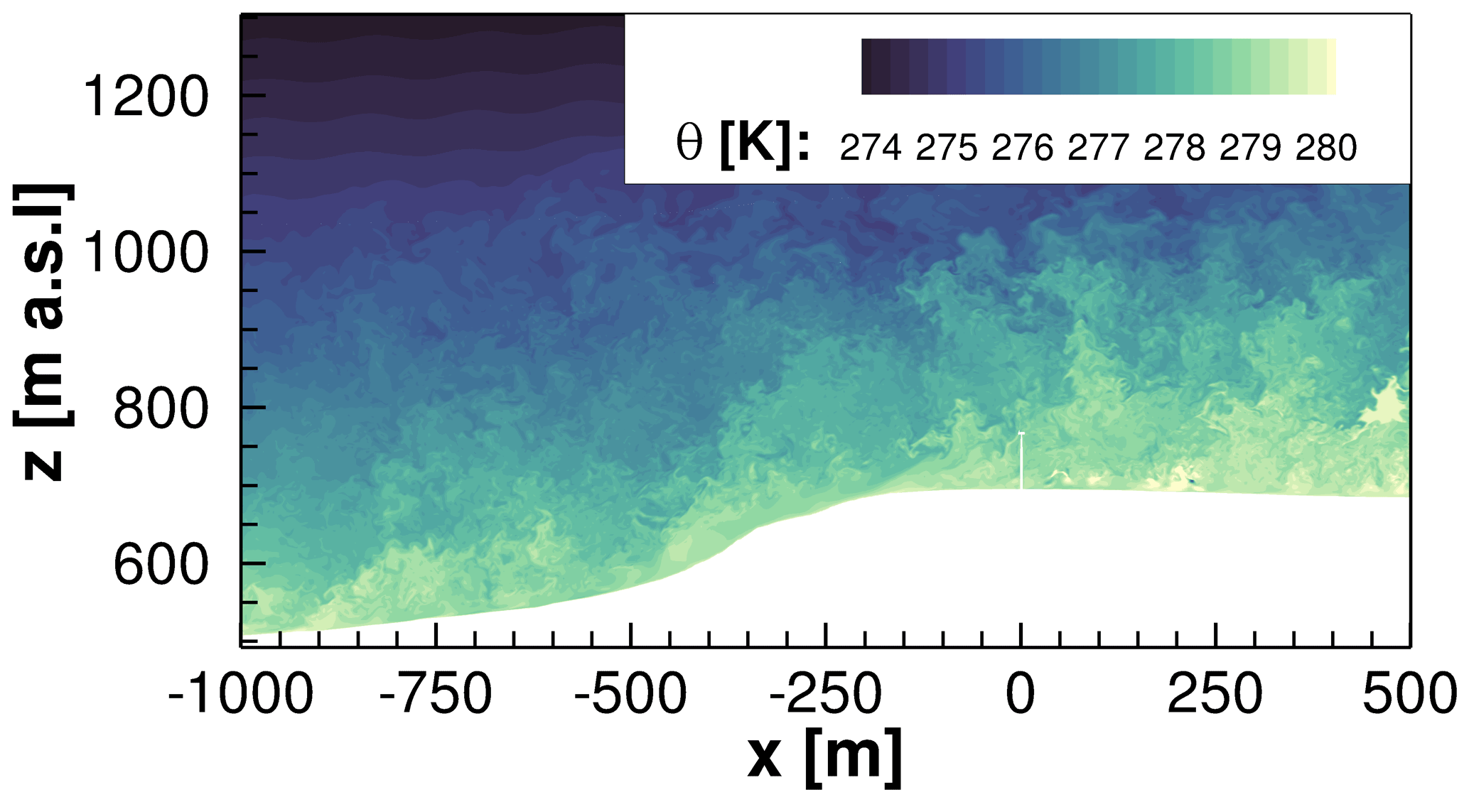
Figure 4 Vertical plane illustrating the development of potential temperature for unstable conditions; wind turbine at x=0 m.

Figure 4 shows a plot of the potential temperature in a xz plane through the 3 D field at an arbitrary time. It illustrates the profile of the potential temperature in the presence of typical unstable conditions in complex terrain with the wind turbine at x=0 m. The plot is intended to serve as an example of the newly implemented feature to consider the impact of potential temperature.

To implement an approach to consider atmospheric stratification, the momentum equations must include the buoyancy force, which depends on the change in potential temperature over height and acts positively directed upward for unstable stratification and negatively directed downward for unstable stratification. For this purpose, the momentum equations are adapted analogously to Churchfield et al. (2014) in Eq. (4).

2.7 Governing equations

The momentum equations are represented by Eq. (4). On the right-hand side of the equation, besides the external force term of the forest model F_F, the buoyancy force is implied. This convective force results from density differences of air parcels (ρ_k) with their surroundings (ρ₀). The reason for these density differences are gradients of the potential temperature.

$$\begin{array}{}\text{(4)}& \begin{array}{rl}& {\displaystyle \frac{\partial \left[\langle \mathit{\rho }\rangle \cdot {\stackrel{\mathrm{̃}}{u}}_i\right]}{\partial t}}+{\displaystyle \frac{\partial \left[\langle \mathit{\rho }\rangle \cdot {\stackrel{\mathrm{̃}}{u}}_i{\stackrel{\mathrm{̃}}{u}}_j\right]}{\partial x_j}}+{\displaystyle \frac{\partial \langle p\rangle }{\partial x_i}}\\ & =-{\displaystyle \frac{\partial \left[{\stackrel{\mathrm{̃}}{\mathit{\tau }}}_{ij}-\langle \mathit{\rho }\rangle \cdot \stackrel{\mathrm{̃}}{u_i^{\prime \prime }{u}_j^{\prime \prime }}\right]}{\partial x_j}}-g_{\mathrm{3}}z{\displaystyle \frac{\partial }{\partial x_i}}\left({\displaystyle \frac{{\mathit{\rho }}_k}{{\mathit{\rho }}_{\mathrm{0}}}}\right)+F_{\mathrm{F}}\end{array}\end{array}$$

3 Results – part 1: case study of general effects

An analysis of the different effects that have a significant impact on the flow field is presented in the first part of the results in Sect. 3. Initially, the focus is on the forested escarpment of the test site. Subsequently, the impact of thermal stratification on the test site is shown, and, finally, the wind turbine is incorporated into the domain.

Through this method, several parameters that influence the flow field at the test site can be examined separately. In the second part of the results in Sect. 4, all effects are combined and applied to a real observed study.

3.1 Effects of the forested escarpment on the flow field

In the following, we investigate the extent to which the flow field is affected by the forest at the wind energy test site. To simulate forests in a highly resolved approach, forest heights and foliage densities must be analysed to model the trees accurately. For this purpose, digital elevation models (DEMs) and digital surface models (DSMs) with 1 m resolution provided by the State Office for Geoinformation and Land Development in Stuttgart (LGL) were used to determine the heights of the vegetation on the test site. In contrast to the DEM, the DSM also includes the topographic aspects of buildings and vegetation in addition to the orography of the terrain.

Figure 5 Comparison of the DEM and DSM models of the test site in complex terrain.

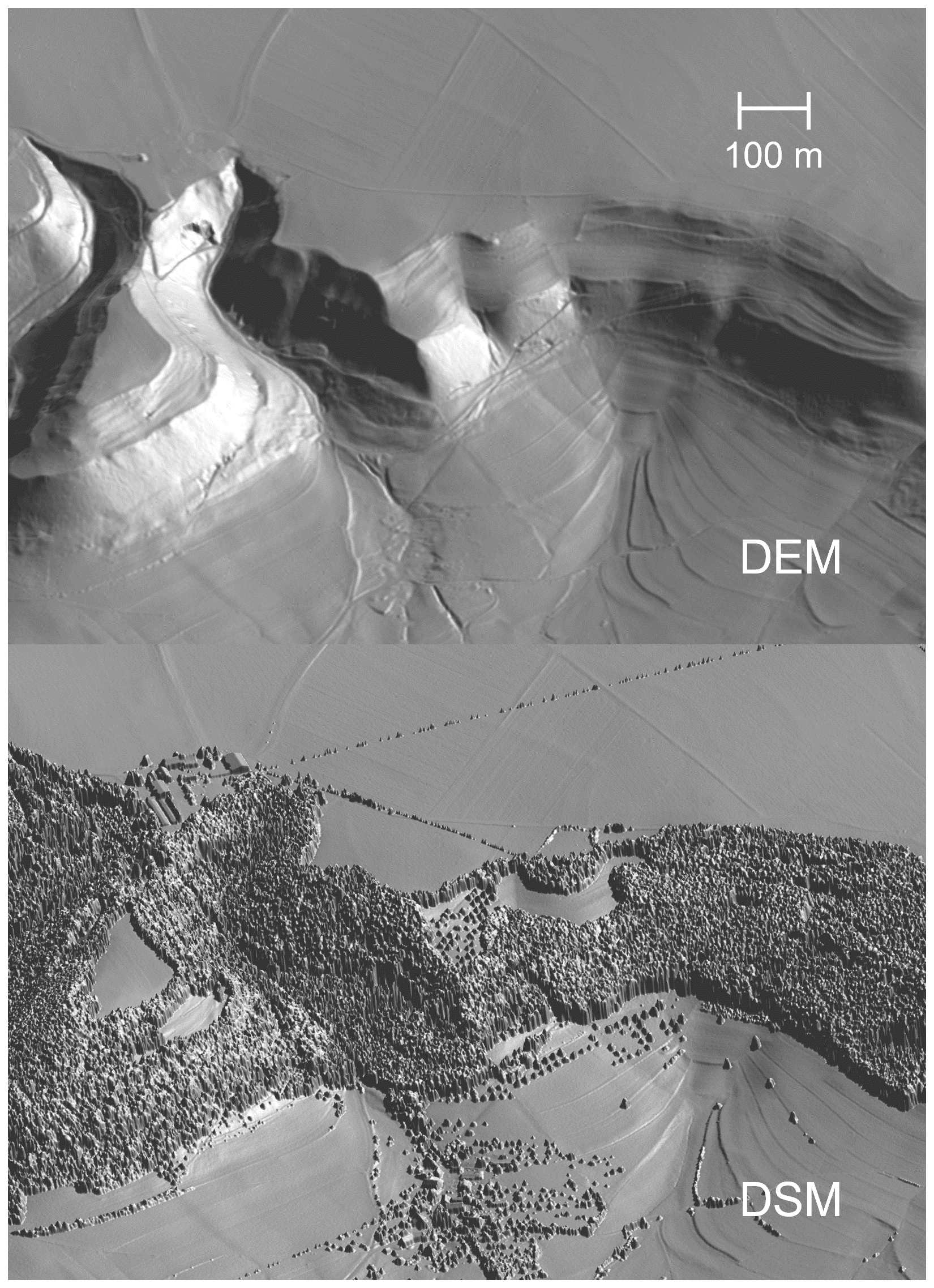
Figure 5 shows the differences between the DEM and DSM models. While the DEM model in the upper image only represents the orography, the DSM model in the lower image can also accurately detect and describe structures such as trees or other obstacles. Thus, the heights of trees and buildings are determined by subtracting the DEM and the DSM model heights. The result is shown in detail in Fig. 6.

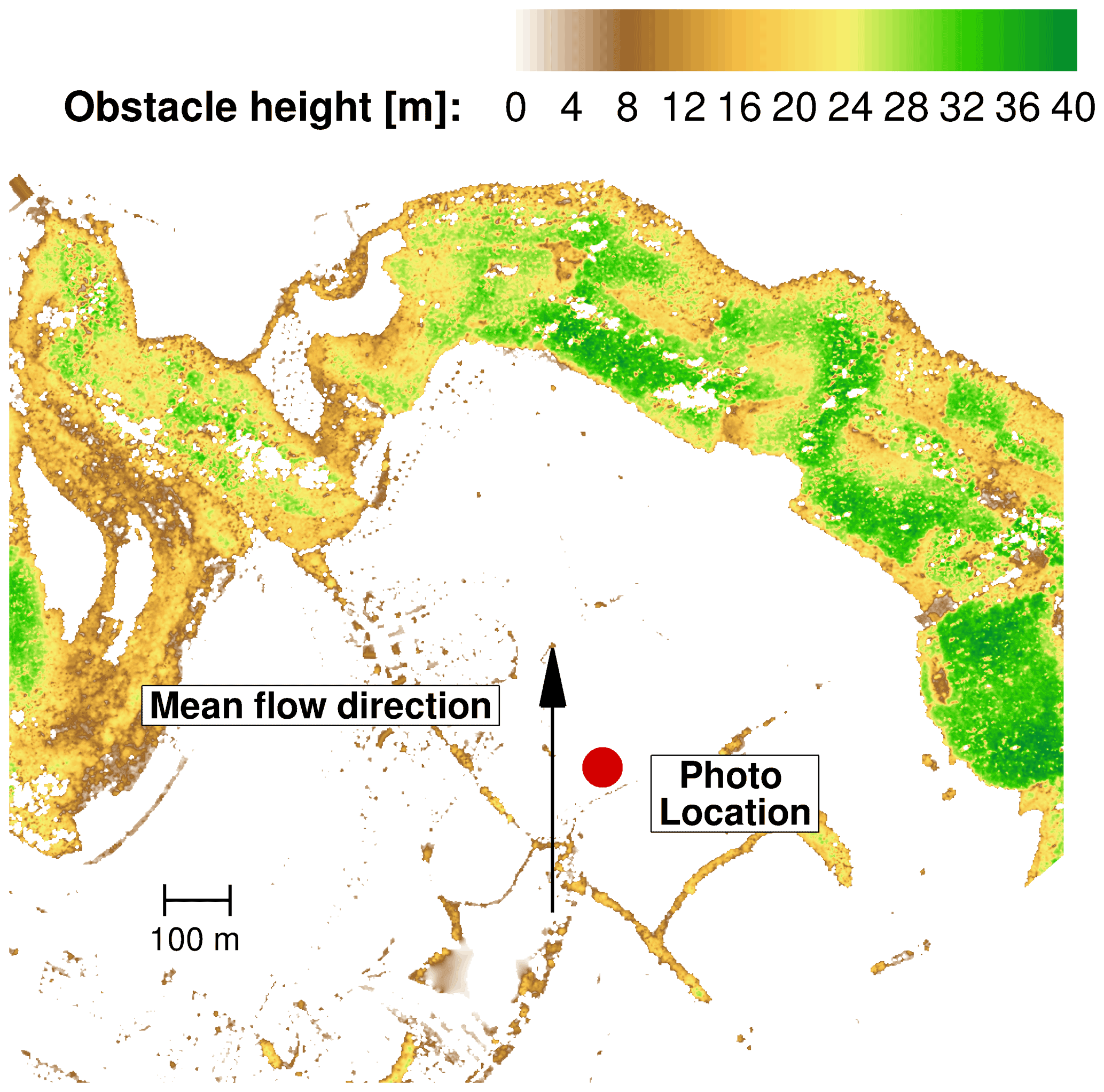
Figure 6 Vegetation and building heights on the test site. The info is used for detailed modelling of the tree heights.

The Albtrauf near Donzdorf is characterised by a mixed forest consisting mostly of beech and spruce, which is typical for most parts of the forests of the Swabian Alps (ForstBW, 2021). There are almost no clearings on the entire escarpment. In general, trees at the test site are 20 to 35 m tall. Regarding the mixed forest, seasonal variations in foliage cover occur that affect the LAI and consequently the flow field downstream of the forested escarpment.

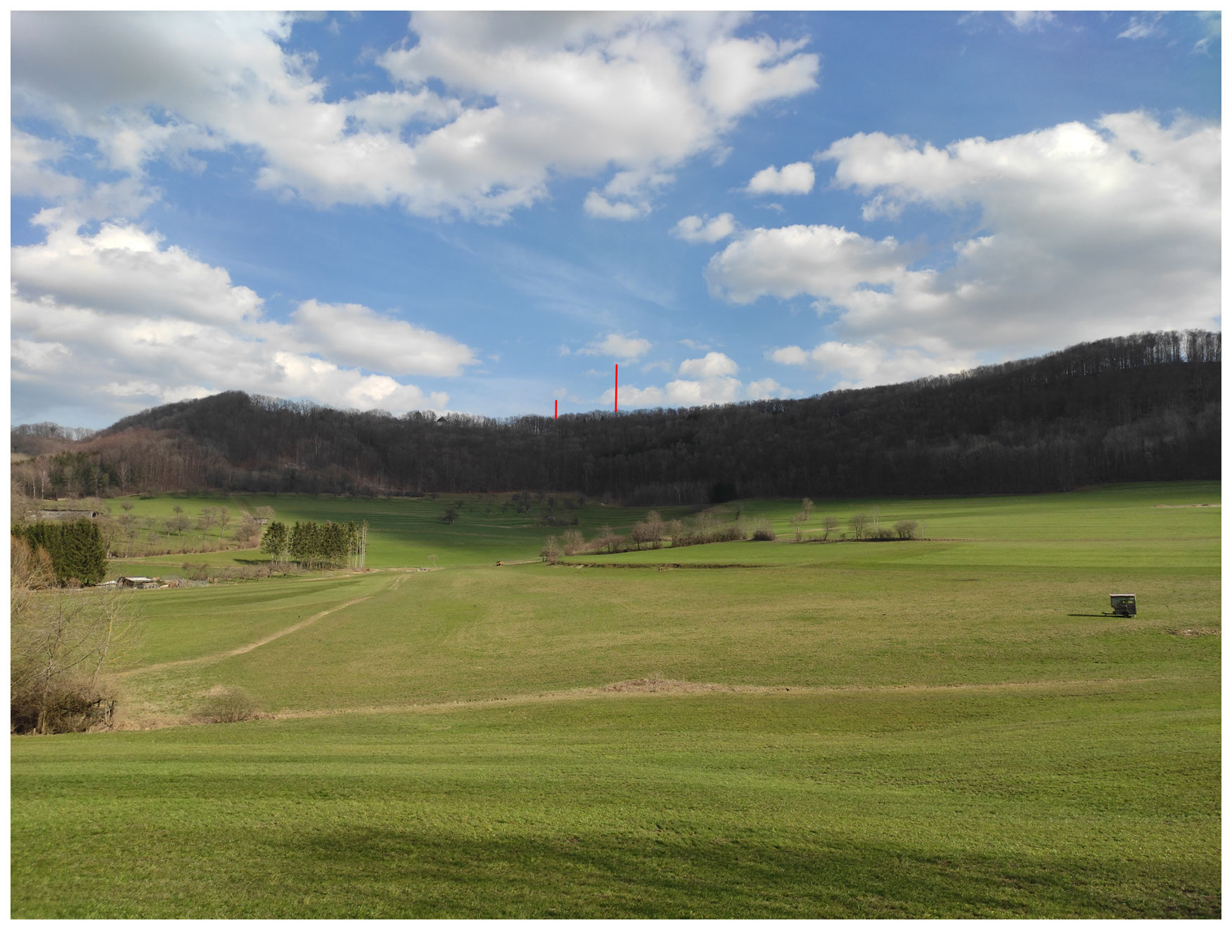
Figure 7 Photo at the position of the inflow plane with a view in flow direction onto the forested escarpment of the test field. Above the forest, the tops of the met masts are visible.

Figure 7 shows a photo of the forested escarpment taken on 26 March 2021 near the position of the numerical inflow plane. The tops of the two met masts are visible in the background on the plateau. For visualisation reasons, the representation of the met masts has been highlighted with red lines. A close look at the photo illustrates how sparsely covered the forest was in the early part of the year. However, the Albtrauf is also characterised by spruce stands, so the winter LAI is approximately 2 m² m⁻² since the trees are typically close together at the escarpment. In contrast, the mixed forest in the summer months is modelled with a mean LAI of 4.5 m² m⁻². The forest heights were modelled analogously to Fig. 6 in the simulations. The used LAI values are specified separately for each simulation.

Emeis (2013) described how the forest cover affects the flow field in flat terrain. A forested escarpment even increases the influence on the local flow field. Thus, the effects of the forested escarpment on the flow field are analysed in detail.

Figure 8 Detailed flow field of the forest in a vertical plane.

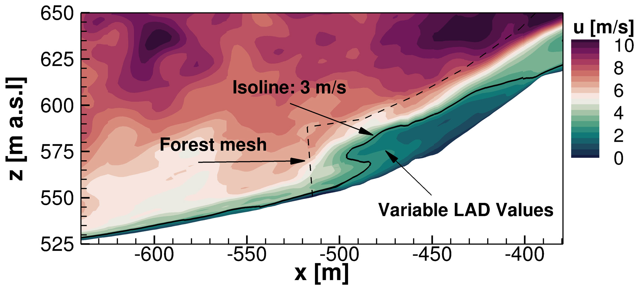
A detailed illustration of the simulation of the forested escarpment is given by Fig. 8. In a vertical plane that also crosses the wind turbine position further downstream, the flow situation at the beginning of the forested escarpment is visible. The forest was modelled with an LAI value of 4.5 m² m⁻², and the flow field shows ambient turbulence with an intensity of 10 % with a mean speed of 8 m s⁻¹ at hub height in the valley with an initial length scale of 40 m, as these values fit well to a situation in the test field at neutral conditions. In addition, the rated conditions of the wind turbine of 11 m s⁻¹ are reached on the test site under these conditions. In the simulation, the corresponding shear (Hellmann) exponent was chosen to be α=0.17. The influence of the forest is evident. The impact in the flow field is highlighted by an isoline representing a velocity of u=3 m s⁻¹. This line indicates how the leaf area density over height was modelled at this position. The forest mesh is sketched with a dashed line to highlight the extent of the forest within the terrain.

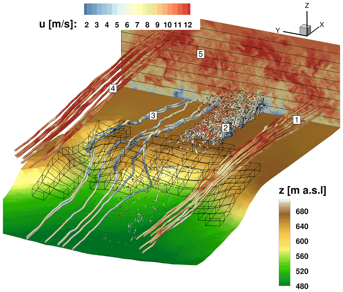
Figure 9 Flow situation in the test field shown in detail with highlighting of five characteristic flow areas.

Figure 9 depicts the flow field of the complete test site for an arbitrary moment. The simulation results show the same inflow parameters as described before. The forested area is marked by black blocks, and different flow regions have been given numbers to analyse the individual flow conditions separately. The respective flow phenomena have been intentionally drawn only in certain regions for clarity, since they occur across the entire width of the domain. Area (1) depicts streamlines coloured analogously to the respective horizontal wind speed. This area shows the lower part of the flow field just above the forest canopy. The colour change from red–white to dark red clearly highlights the typical effect of accelerating flows over hills or ridges. This area also represents the flow region that mainly crosses the rotor plane. Downstream of the escarpment at hub height, the wind reaches a speed of 11 m s⁻¹. This means that the speed increase at the hub height due to the escarpment is 3 m s⁻¹. Area (2) illustrates turbulent structures using the λ₂ vortex criterion. This emphasises the strong mixing of turbulence structures in the wake of the forest. There, considerable low axial velocities and high standard deviations occur. The turbulence is further amplified by the superposition of the turbulent forest wake with the accelerated flow from area (1). A flow region results that comprises high turbulence intensities and large velocity differences. Flow region (3) visualises streamlines in the near-ground region crossing the forest. The blue colouration of the streamlines illustrates the reduction of wind speed due to the forest. Besides, because of the orography and the different leaf area densities above the height and width of the heterogeneous modelled forest, these streamlines are strongly curved and exhibit locally large changes in direction. The shear layer between the flow regions (1) and (3), which exhibits large velocity differences, amplifies the generation of turbulent fluctuations. This is visible for region (2). The same effect has already been analysed and explained by Dupont et al. (2008). Flow region (4) shows the upper flow field a few hundred metres above the ground. There the streamlines are no longer inclined and the influence of the orography is negligibly small. Therefore, the flow does not accelerate when streaming over the escarpment. The small curvatures of the streamlines and velocity changes are only caused by atmospheric turbulence. Whereas the acceleration of the flow field in area (1) caused differences of Δu=3 m s⁻¹, the analyses in this area showed that the small curvatures of the velocity in this upper flow field are in the range of $\mathrm{\Delta }u=\pm \mathrm{0.4}$ m s⁻¹. This statement can also be qualitatively verified by the colour changes of the streamlines. Area (5) depicts a plane on the flat plateau of the test field, which is perpendicular to the flow direction and captures the horizontal wind speeds. This provides a view of the turbulent flow field with all the effects described previously.

From Fig. 9 it can therefore be shown that in complex terrain many different orographic and topographic effects influence the flow field and thus the inflow of wind turbines. In particular, the wake of a forested escarpment, with trees reaching the plateau on top of a slope, influences the flow field to a great extent.

The above-mentioned influences are based on simulations of summer months with an average LAI of 4.5. A variation of the leaf area densities and a comparison of the influences on the test field will be investigated in the following by using the same inflow conditions.

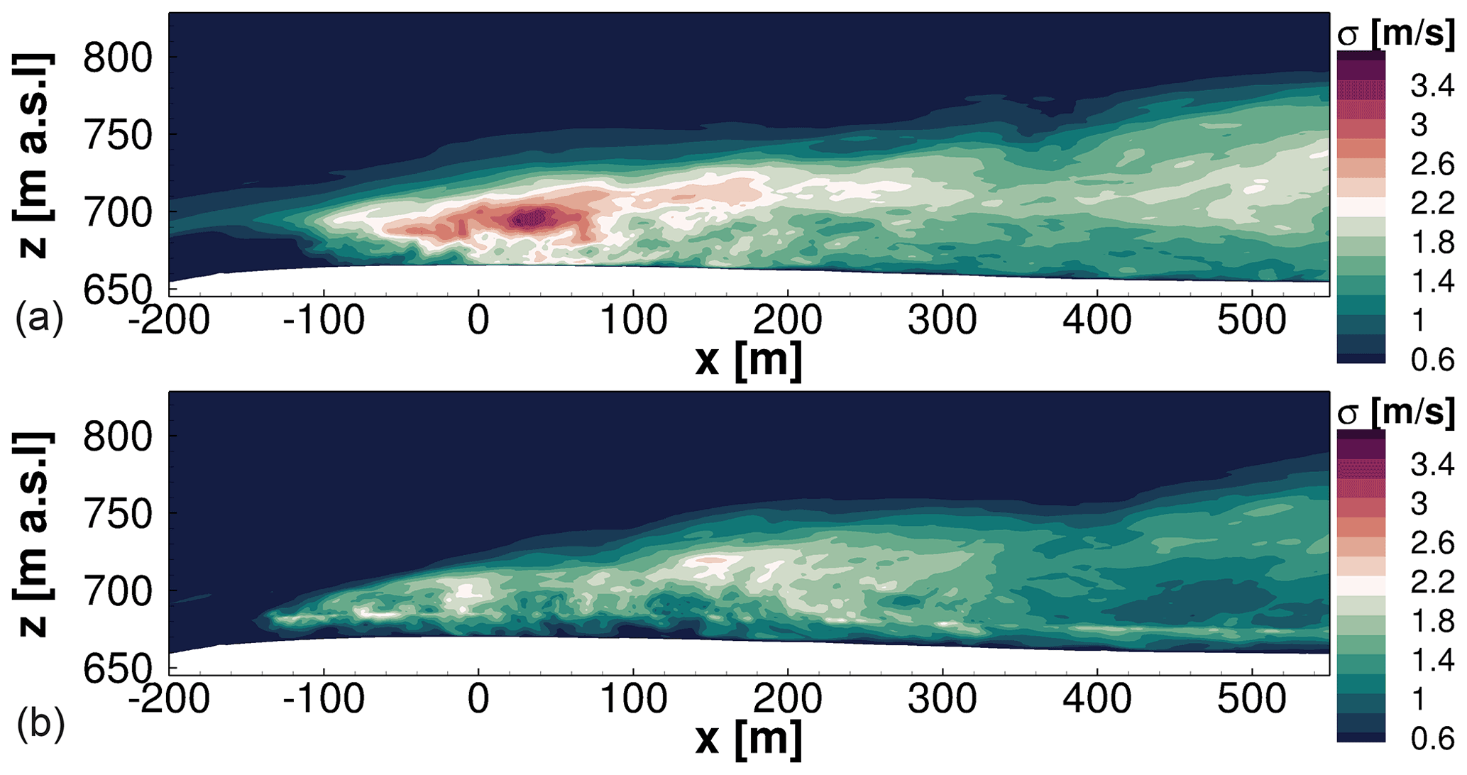
Figure 10 Standard deviation of horizontal velocity in forest wake for different leaf area indices. (a) LAI =4.5 for foliage cover in summer. (b) LAI =2 for foliage cover in winter.

The standard deviations of the horizontal velocity in the wake of the forest on the flat plateau of the test site with the corresponding LAI values for summer and winter months are shown in Fig. 10. The evaluation of the standard deviation is more illustrative than the evaluation of T_i because of the vertically strongly changing mean wind speeds due to the forest near the ground and the strongly accelerated area above due to the escarpment. For the evaluation, the respective flow fields were averaged over 4 min, which means a suitable averaging period below the micrometeorological peak in the spectrum according to Van der Hoven (1957). Further, this is a time period that is similar to subsequent evaluations of wind turbine simulations and is still appropriate for the high temporal and spatial resolution. The upper plot demonstrates the standard deviation in summer months with an LAI of 4.5 m² m⁻² and the lower plot for winter months with an LAI value of approximately 2 m² m⁻². Using these values was valid because of the spruce stands on the escarpment. Lower values than 2 would be typical for pure deciduous forests in the winter months.

At first glance, significant differences of the standard deviation σ become apparent. The higher leaf area densities in the summer months result in stronger amplification of turbulence and consequently in significantly larger standard deviations than in winter months. Especially in the turbine's area at x=0 m, the fluctuations are significantly lower for the sparsely covered forest. It is worth mentioning that the propagation of the standard deviation behaves analogously for both forest covers. This means the turbulence is more amplified by the denser forest, but the forest wake expands to similar ranges in height and width (for the same wind conditions) in the summer and winter months. Consequently, the forest effect is measurable at similar heights for different foliage densities. However, the atmospheric boundary layer in the forest wake will recover more quickly further downstream for the sparsely covered forest due to lower turbulence intensities.

3.2 Effects of thermal stability on the flow field

Next, the influence of thermal stratification on the flow field is analysed. Three simulations with the same inflow conditions and turbulence characteristics are compared. However, the buoyancy varies because of different thermal stratification conditions. As described in Sect. 2.6, the inflow conditions and turbulence characteristics differ significantly for stable and unstable conditions, which was intentionally neglected for the analyses of the influence of the forest wake on the flow field at different stabilities in complex terrain. The following results, therefore, aim exclusively to explain how thermal effects can affect flow fields. The T_i for each case was set to 8 % at hub height. Since the wind turbine is the focus of these analyses, the reference T_i was always set at hub height. The results were assessed at the same time or averaged over a period of 4 min.

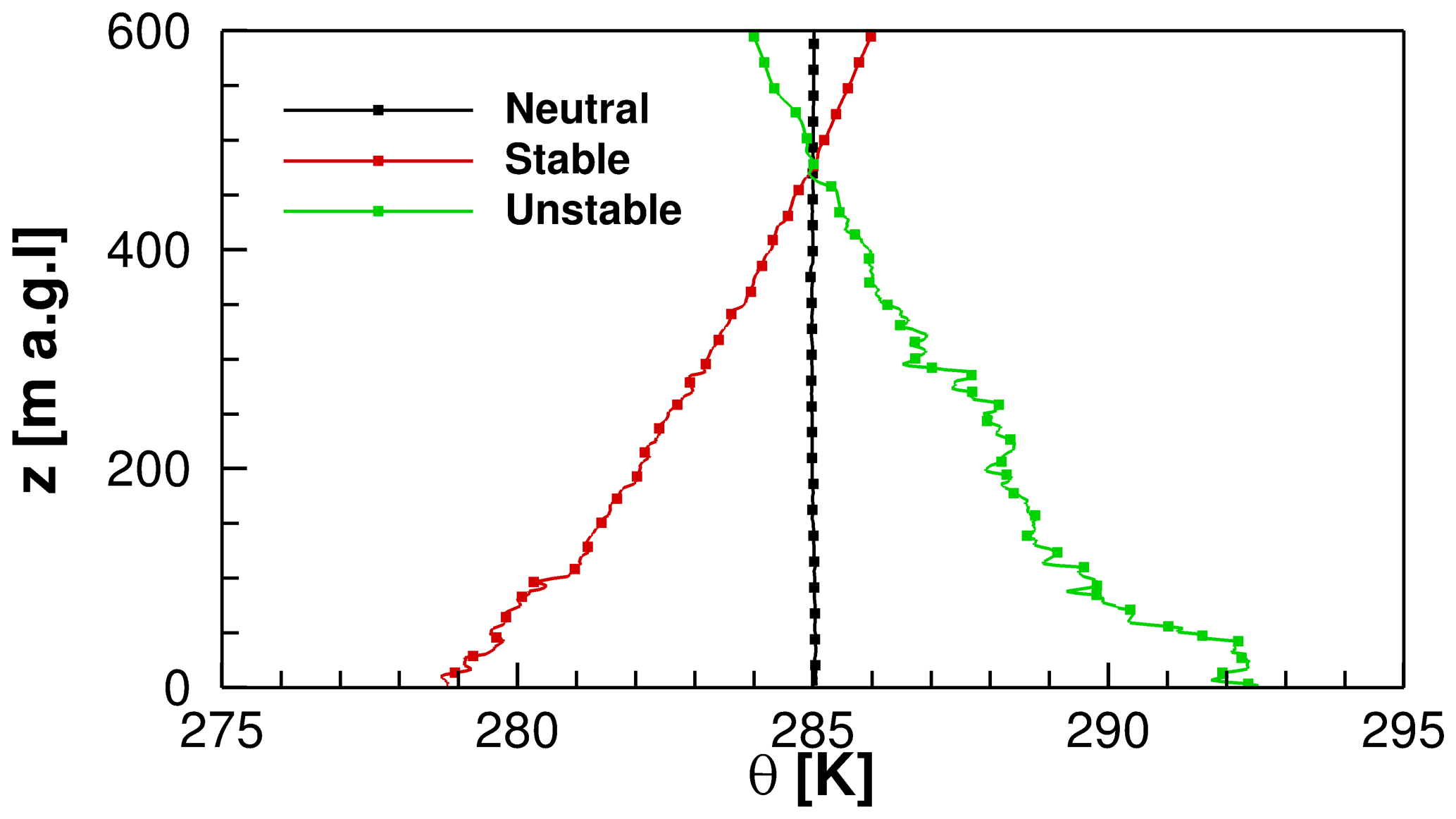
Figure 11 Profiles of the potential temperature of the three atmospheric stratification conditions extracted from their respective flow fields.

Profiles of potential temperature extracted at position $x=-\mathrm{750}$ m in the valley upstream of the escarpment are shown in Fig. 11. These three curves illustrate simulations of neutral, stable, and unstable stratification, respectively. The depth of the atmospheric boundary layer was set to 1000 m in the simulations, and the inversion strength was $\frac{\partial \mathrm{\Theta }}{\partial z}\approx \mathrm{0.009}$ K m⁻¹. The gradients of the potential temperature reveal that these are quite strong cases of atmospheric stability. Thermal stability can be cast in terms of reciprocal M-O length ${L_{\mathrm{MO}}}^{-\mathrm{1}}$ ($P\propto \exp (-|{L_{\mathrm{MO}}}^{-\mathrm{1}}{|}^{\mathrm{2}/\mathrm{3}}$)). The probability distribution P was determined analogously to the procedure described in Kelly and Gryning (2010). This yielded a probability of occurrence of about P(${L_{\mathrm{MO}}}^{-\mathrm{1}}{|}_{z=\mathrm{10}\mathrm{m}}$) ≈1.8 % for the range of the strongly stable conditions present here with ${L_{\mathrm{MO}}}^{-\mathrm{1}}$ ≈0.06 and a probability of occurrence of about P(${L_{\mathrm{MO}}}^{-\mathrm{1}}{|}_{z=\mathrm{10}\mathrm{m}}$) ≈1.1 % for the range of the strongly unstable conditions with ${L_{\mathrm{MO}}}^{-\mathrm{1}}\approx -\mathrm{0.07}$. The depicted lines belong to particular stratification conditions, which are also illustrated in Fig. 12.

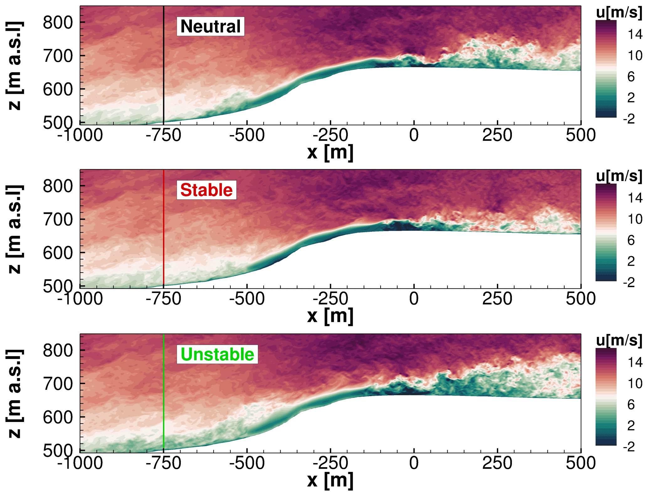
Figure 12 Snapshots of extracted vertical slices of the flow field under different stratification conditions.

In Fig. 12, three snapshots of the simulation results are illustrated simultaneously in different stability conditions. Based on the gradient of potential temperature from Fig. 11, the buoyancy is calculated. All three cases are investigated using the same inflow conditions. This is not the case in nature, because thermal stability also affects the properties of turbulence, such as its intensity, length scale, and dissipation. The study, however, in general aims to assess the effects of a pressure-driven ABL, where a buoyancy acts due to the vertical gradients of the potential temperature.

The flow field in neutral conditions is shown in the upper plot. Results for stable and unstable conditions are shown analogously in the middle and lower illustrations. It can be observed that atmospheric turbulence changes due to buoyancy in the flow region close to the inflow between $x=-\mathrm{1000}$ and $x=-\mathrm{600}$ m. The forest wake even amplifies buoyancy effects. In the wake of the forest, the influences of buoyancy become evident. Using the flow field for neutral conditions as a reference case, it is noticeable that stable stratification suppresses the mixing of the forest wake with the ambient turbulence. Consequently, the wake exhibits smaller fluctuations and does not extend to high altitudes. Unstable stratification has the opposite effect. Thus, the wake and ambient turbulence are mixed and propagated to larger heights, resulting in higher turbulence intensities. Ultimately, unstable conditions influence the test site and the wind turbine inflow more than other conditions, which will be emphasised hereinafter.

Figure 13 Standard deviation of horizontal velocity in the forest wake for different stratification conditions.

The standard deviations σ of the horizontal velocity are displayed in an enlarged graph of the forest wake in Fig. 13. In a 4 min time window, standard deviations were evaluated. The upper plot shows the flow field for neutral stratification, the middle plot for stable stratification, and the lower plot for unstable stratification. Again, neutral stratification is chosen as a reference case. Further downstream, the standard deviation decreases, indicating a reduction in turbulent fluctuations, although the wake extends to higher altitudes. For stable stratification, the standard deviations in the forest wake decrease compared to neutral conditions. This suppresses turbulence, causing the σ values to decrease significantly. On top of that, the wake does not extend to higher altitudes. A similar result was obtained by Desmond et al. (2017) both numerically and in wind tunnel measurements. The opposite effect is again evident in the lower plot for unstable stratification. The standard deviation decreases with increasing distance downwind of the forest, but the turbulence in the forest wake spreads at much higher altitudes than for other conditions.

Transverse planes at the wind turbine position will further emphasise these effects as can be seen in Fig. 14.

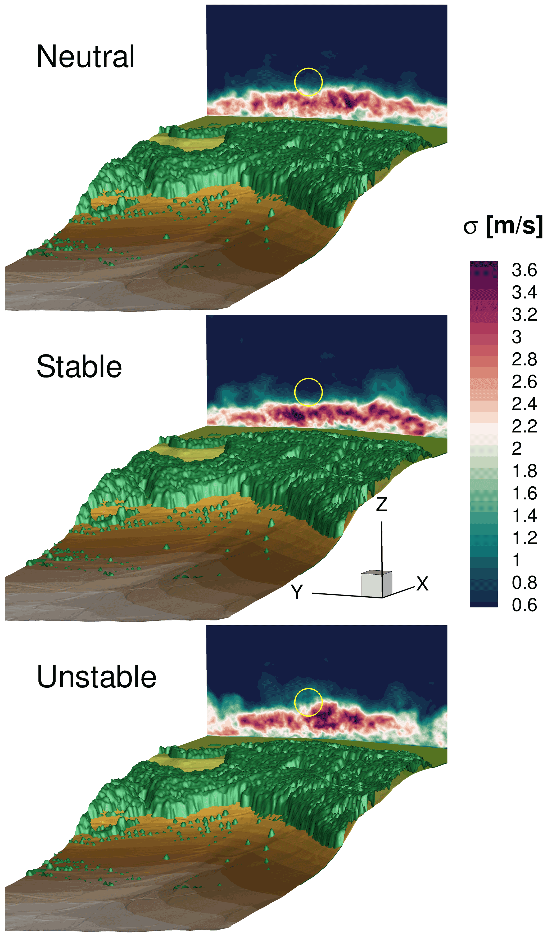
Figure 14 Standard deviation of the horizontal velocity at the wind turbine position. The rotor position is outlined by the yellow circle.

Figure 14 depicts the flow field at the turbine position for neutral, stable, and unstable stratifications. Here, the standard deviation $\mathit{\sigma }=\sqrt{{\mathit{\sigma }}_u^{\mathrm{2}}+{\mathit{\sigma }}_v^{\mathrm{2}}+{\mathit{\sigma }}_w^{\mathrm{2}}}$ is analysed, which was evaluated over 4 min. In particular, the influence of the vegetation on the flow field at different stability conditions will be further investigated. Besides the plane at the turbine location, the forested areas are also shown. In the contour slice, the rotor area is sketched with a yellow circle. This is supposed to show how the wind turbine is affected by the flow field of the forest wake for different stabilities. The buoyancy force has a very large impact on the mean flow field. As compared with other thermal conditions, fluid mixing in the forest wake spreads over the entire width to higher altitudes for unstable stratification. Thus, the forest wake also crosses the rotor plane. This dominant effect is visible in the lower plot. For neutral stratification, vortex structures detaching from the forest only sporadically cross the lower half of the rotor. For stable stratification, there are only scattered turbulent structures influencing the rotor. On average, for stable conditions, most of the rotor remains unharmed by the forest wake.

3.3 Forest effects on the wind turbine

In the following, interaction of the forest wake and the wind turbine is investigated for neutrally stratified conditions.

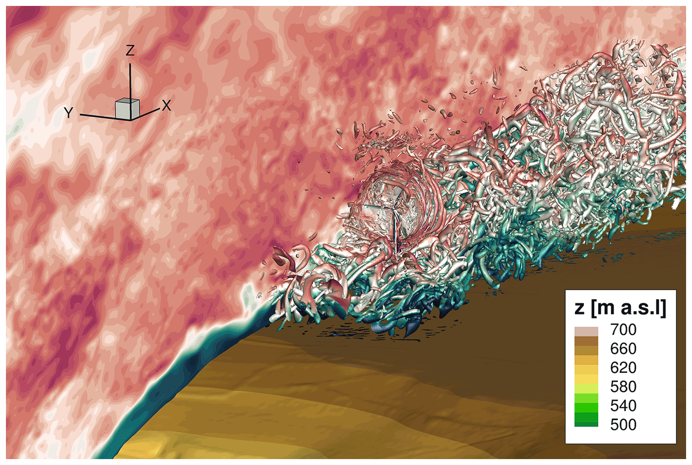
Figure 15 Snapshot of the interaction of the wind turbine with the forest wake and the ambient turbulence.

Figure 15 shows an unsteady flow situation in which the forest wake and atmospheric turbulence interact strongly with the wind turbine and its wake. The wind turbine was incorporated into the computational domain of the same simulation as in Fig. 9. The initialised fully meshed wind turbine was subsequently simulated over a period of a few rotor revolutions in order to eliminate numerical disturbances that arise when the turbine is incorporated into the numerical domain. After 25 further revolutions, this plot was extracted. A vertically oriented plane of the local velocity was extracted to illustrate the flow field at the topography. Additionally, λ₂ structures of turbulence are shown to indicate the strong interaction of the forest wake, the ambient turbulence, and the turbine. After the propagation of only a few rotor revolutions, the blade tip vortices break down into smaller turbulent structures. Further downstream, there is a turbulent low speed area, where the turbine wake and the forest wake can no longer be distinguished. More detailed analyses of this effect are presented below.

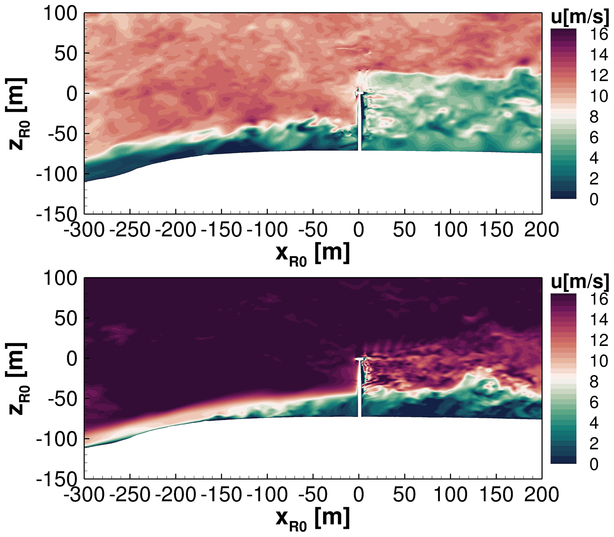
Figure 16 Vertical planes of the interaction of forest wakes, ambient turbulence, and wind turbines for two different flow cases.

In the following section, two different flow and vegetation conditions will be analysed to develop a physical understanding of the topography–forest–turbine interaction. Figure 16 shows the interaction of the forest wake and the wind turbine. In the upper plot, the same flow situation as described before in Fig. 9 is analysed, which reaches rated turbine conditions of 11 m s⁻¹ at hub height with a T_i of 10 %. Again, this study is intended to show a summer situation with relatively high wind speeds. Here, the forest is completely leafy and accordingly has an LAI of about 4.5. Occasionally, vortex structures of the forest wake cross the rotor plane, which leads to large velocity fluctuations that may influence the rotor loads and the turbine performance negatively. In the upper plot, the dense forest causes vortex shedding at the canopy, which can randomly affect the inflow onto the wind turbine. A large area of reduced wind speeds is presented from the upper blade tip to the ground downstream of the turbine. The forest wake quickly mixes with the turbine wake, leaving a large common wake area.

In the lower plot, a comparable vertical plane is shown at higher wind speeds. This is a simulated real observed flow scenario from 31 March 2019 at 23:00 CET at the test site with average wind speeds of 16.5 m s⁻¹ at hub height. A T_i of 9 % and a length scale of 35 m was measured from the met mast at hub height, which was adjusted to the flow situation in the valley and then used as inflow data for the FLOWer simulations. As the forest is not completely leafy in spring, it was modelled with an averaged LAI of 2.8. Because of the high wind speeds, the rotor blades are provided with larger pitch angles, which is the reason why the velocities of the wake are not reduced as much by the turbine as in the plot above. By contrast, the inflow of the wind turbine is less affected by the sparsely covered forest, but downstream of the wind turbine a strong interaction between the forest wake and the turbine wake is readily apparent. Caused by the higher velocity differences of turbine wake and forest wake, they do not mix to the same extent as in the upper plot of Fig. 16. However, the small velocities in the forest wake affect a deflection of the turbine wake. There is a noticeable vertical wake deflection at x=130 m, which strongly influences the turbine wake propagation. As a result, the forest wake and the turbine wake do not mix as strongly as they do in the upper plot, but the speed differences of the turbulent structures result in significant deflections. Thus, neutral stratification and different leaf area densities result in large forest–turbine interactions, which have a significant impact on inflow and wake.

3.4 Thermal stability effects on the wind turbine

In the following, influences of different stratification conditions with consideration of the wind turbine are compared. For this study, the influence of vegetation will be neglected to capture the effects of buoyancy on the inflow and wake of the wind turbine separately. For this purpose, the inflow conditions from Figs. 12 and 13 were again used. With integrating the turbine into the flow field, the forest was removed as just described to investigate only the influence of buoyancy and ambient turbulence on the wind turbine in complex terrain.

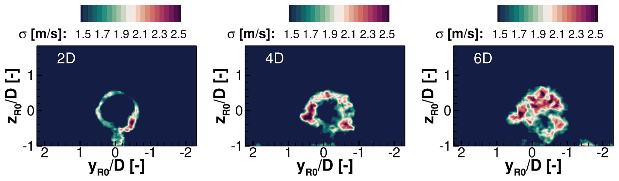
Figure 17 Standard deviations of the wake for stable stratification in transverse planes several rotor diameters (2 D, 4 D, and 6 D) downstream of the wind turbine

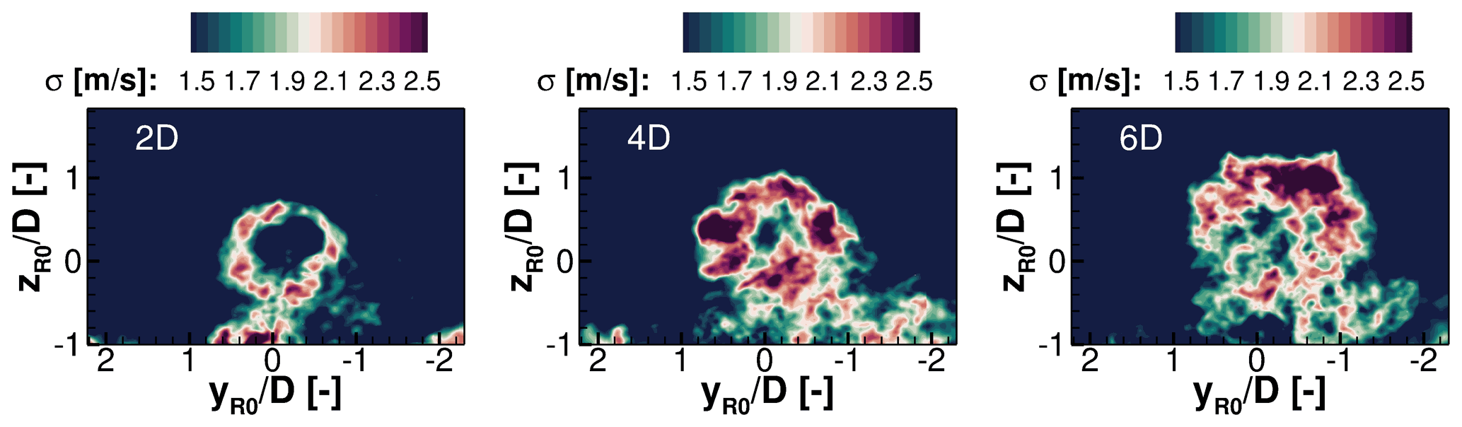
Figure 18 Standard deviations of the wake for unstable stratification in transverse planes several rotor diameters (2 D, 4 D, and 6 D) downstream of the wind turbine.

Standard deviation σ ($\mathit{\sigma }=\sqrt{{\mathit{\sigma }}_u^{\mathrm{2}}+{\mathit{\sigma }}_v^{\mathrm{2}}+{\mathit{\sigma }}_w^{\mathrm{2}}}$) of planes perpendicular to the flow direction several rotor diameters (2 D, 4 D, and 6 D) downstream of the wind turbine are illustrated in Figs. 17 and 18. Figure 17 represents the wake cross sections for the simulations under stable conditions and Fig. 18 for unstable stratification. Through the standard deviation σ, the shape of the wake and the mixing with the ambient turbulence are explained. It becomes apparent that further downstream the fluctuations of the wake are considerably larger for unstable stratification than for stable conditions. Comparing the standard deviation σ in Fig. 17 with Fig. 18, it is recognisable that already 2 D downstream of the turbine the plots look entirely different. In this region primarily the blade tip vortices cause these high values of the standard deviation. For unstable stratification, the vortices spread out into significantly wider areas, whereas for stable stratification the wake keeps its circular shape longer. Further downstream, it can be assumed that the wake decays for unstable conditions more quickly, due to vortex breakdown, as analysed by Troldborg et al. (2014). In stable stratification, the vortex decay will occur comparatively further downstream due to suppressed mixing, which is evident from the standard deviation at all planes.

4 Results – part 2: real case study on 10 March 2021

In the second part of the results, the previously described effects on flow fields in complex terrain are investigated combined for a case study based on observed conditions. For this study, a 5 min time period of the measurement data from 10 March 2021 at 11:30 CET was extracted to generate inflow data in the valley. This was then propagated through the domain and compared to the experimental data. On the plateau, the flow direction is west-northwest, which corresponds with the predominant wind direction at this site. The atmosphere was slightly unstable, and the forest was not leafy because it was springtime (winter conditions). The depth of the ABL was set to 300 m height, which admittedly was chosen rather shallow for unstable conditions even in the present winter conditions, but for the focus of these analyses, which due to the wind turbine lies on the area close to the ground, this is nevertheless sufficient. The turbulence and velocity profiles were measured by the met mast. To obtain the velocity profile at the inflow plane, the measurement data were adjusted to the flow field in the valley. This means that the measured turbulence statistics of the met mast on the test site were used to generate synthetic turbulence in the valley. This turbulence will be superimposed in the valley with a sheared velocity profile, which is adapted in such a way that the acceleration of the wind due to the escarpment fits to the time-averaged measurements of the met masts.

The quantitative adjustment of the inflow velocity field from the measured data downstream of the escarpment can be described from empirical values as follows. The previous analyses of the flow field showed that in the investigated terrain on the Swabian Alps, speed-ups of 35 % to approximately 60 % result at hub height compared to the velocities in the valley at the same reference height. The relative speed-up tends to be higher for lower wind speeds in the valley. This demonstrated the advantage of using the escarpment for wind energy at the test site. For a reference velocity of 8 m s⁻¹ in the valley and 11 m s⁻¹ on the test field plateau the relative speed-up is approximately 37.5 % and at 16.5 m s⁻¹ the speed-up was 35 %, as the simulation in Fig. 16 showed. For this current situation the reference velocity was 7.7 m s⁻¹ at hub height, which results in a speed-up of approximately 60 % compared to the valley situation.

This procedure resulted in a reference velocity u_ref=4.8 m s⁻¹ at hub height z_ref=72 m with an Hellmann exponent α=0.2 at the inflow plane. The synthetic turbulence for this purpose was generated with a turbulence intensity of T_i =15 % analogous to the measurement results of the met masts. The used length scale was 42 m, which is consistent with findings of Peña et al. (2010) and Sathe et al. (2013) for slightly unstable conditions at comparable wind speeds. The anisotropy Γ was set to 2.9 and the dissipation factor $\mathit{\alpha }{\mathit{ϵ}}^{{}^{\frac{\mathrm{2}}{\mathrm{3}}}}$ resulted in 0.03 m${}^{\mathrm{4}/\mathrm{3}}$ s⁻², which fits to the studies of Chougule et al. (2016) and Kelly (2018). Because of insignificant wind veer, the Coriolis force is ignored. At the heights investigated, the maximum difference from the main wind direction was 5.5 % in the averaged time window. Therefore, the wind veer was classified as negligible.

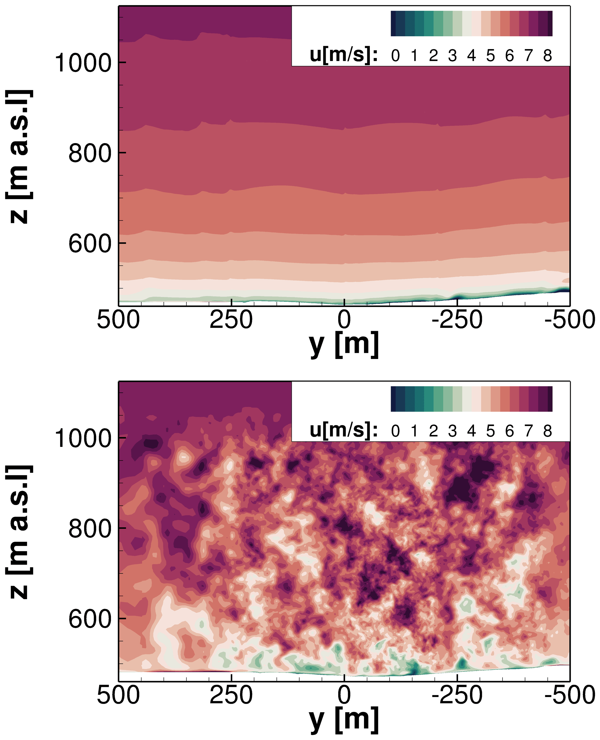
Figure 19 Generation of turbulence from the met mast data of 10 March 2021 and the resulting turbulent flow field at the inflow.

The generated unsteady inflow plane is shown in Fig. 19. The used velocity profile at the inflow is illustrated in the upper plot. This above-the-ground extracted velocity profile is superimposed with the generated synthetic turbulence by source terms. The resulting flow field is shown in the lower plot at a position two length scales downstream of the inflow plane. This transient turbulent field is propagated through the domain. After one complete flow through the whole domain, the evaluation, as well as the averaging of the simulation, was started in order to compare it with the met mast data as shown by Fig. 20.

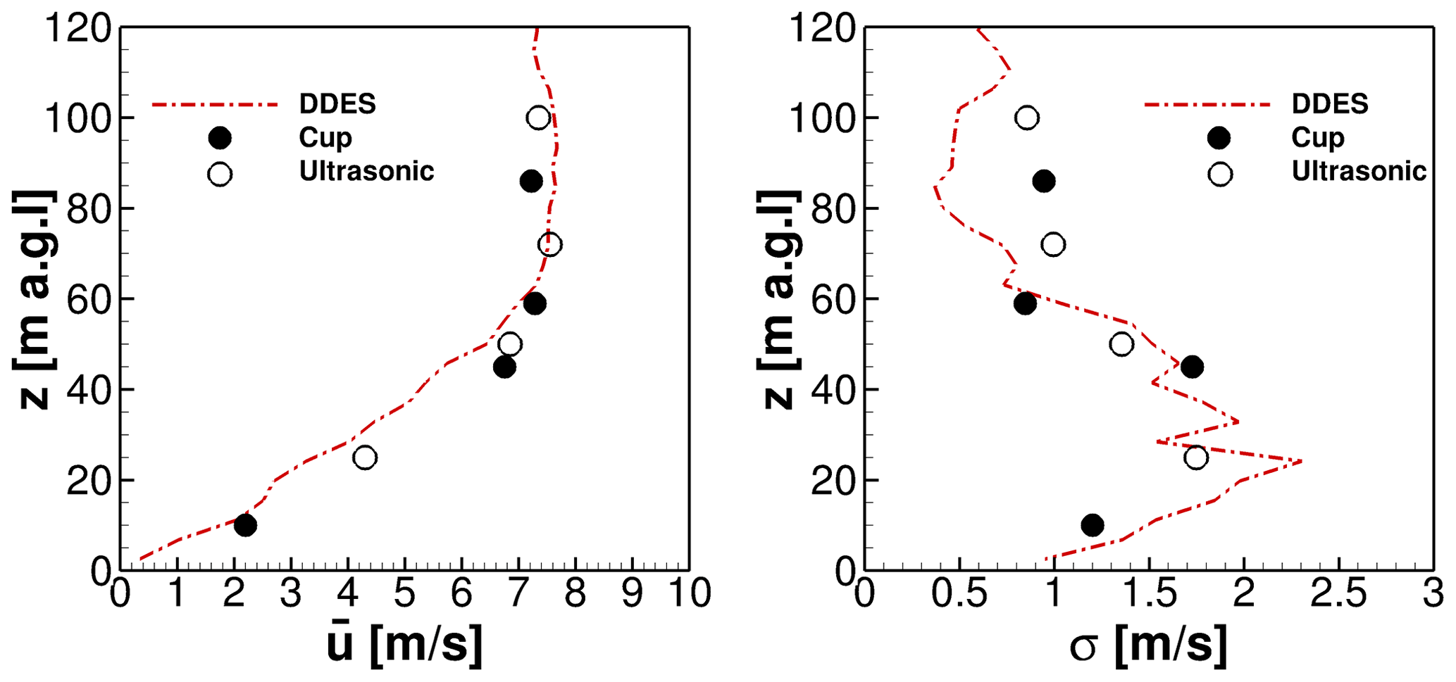
Figure 20 Averaged flow quantities of the simulations in comparison with measured mast data from 10 March 2021.

Figure 20 illustrates the comparison of simulated flow quantities compared with experimental data of the first met mast. Both the measurements and the simulations show results, which are averaged over 5 min. The mean velocity profile at the met mast position is depicted in the left plot. The forest wake with reduced velocities near the ground causes the almost linear increase of the curve until 50 m a.g.l. In the upper part of the velocity profile near the rotor plane and above, there is very little shear of the wind speed. The wind speed remains almost constant over the height, which can be explained by the speed-up over the terrain in lower areas, whereas the upper flow field is less influenced by the orography. This effect has also been illustrated by flow regions (1) and (4) in Fig. 9. Besides, the shear is suppressed by the convective conditions in this situation, because the buoyancy force drives air masses upward. It is noticeable that the numerical results show a decent agreement compared to the measured data. The deviation of all measurement points to the simulated results remains in a range of ±1 m s⁻¹. The graph of the standard deviation σ above the height is shown in the right plot. Up to 60 m above the ground, the standard deviation and consequently the turbulence is significantly increased, which is shown in both the simulation and the measured data. The forest wake, which extends to higher altitudes because of the unstable conditions, primarily causes this effect. A stronger mixing of the ambient turbulence and the forest wake is the result. In this region, the examined turbulence properties match well with the CFD simulations. At higher altitudes, there are deviations of the numerics and the measured data. This can probably be explained by the evaluation period in the simulations, whereby the synthetic turbulence generated stochastically via the Mann model did not exactly match the real turbulence characteristics. These turbulent data were fed into the inflow plane in the valley more than 1000 m upstream of this evaluation position.

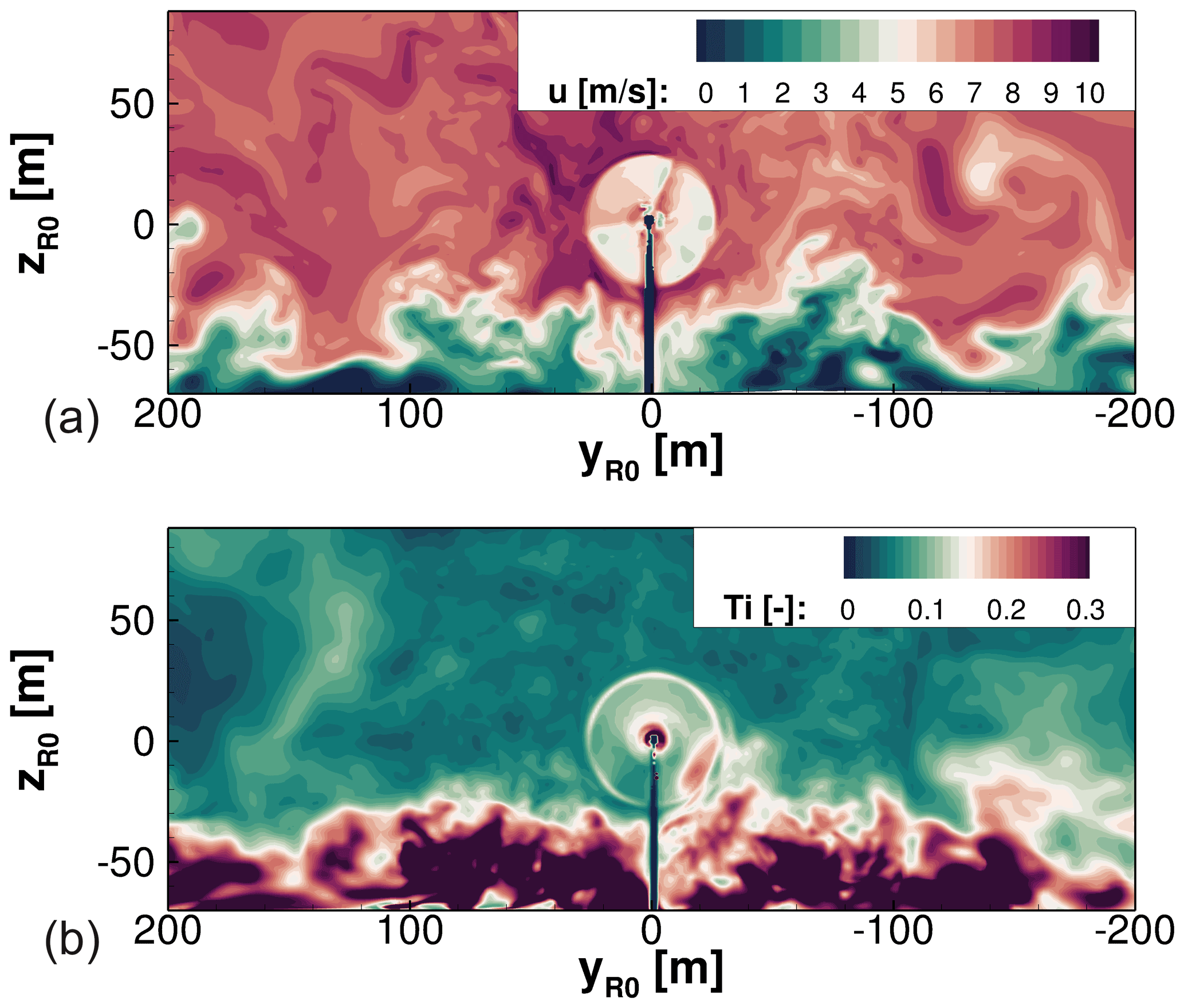
Figure 21 Flow situation at the wind turbine position for unstable conditions on 10 March 21. (a) Instantaneous flow field. (b) Turbulence intensity of the flow field.

A plane through the rotor position is visualised in Fig. 21. In the upper plot, the flow field at an arbitrary moment in time is shown. The interaction of the turbine rotor, the ambient turbulence, and the turbulent wake of the forest are shown. The situation depicts the flow field 65 revolutions after the rotating turbine has been integrated into the flow field. From the turbulent structures of the forest wake, which propagate heterogeneously and expand to different heights, it becomes evident that with increasing time, detaching vortex structures with low horizontal velocities cross the rotor plane. Investigating the lower plot, the turbulent inflow onto the turbine is characterised. The turbulent forest wake extends on average into heights of 45 m. The significantly increased T_i results from fluctuations at low mean velocities in the forest wake. If these structures flow through the rotor plane, the inflow will be significantly affected. This influences the loads, the power, and the wake. Especially in the lower-right rotor position, the high T_i caused by the forest wake is remarkable. The effect on the wake is explained in Fig. 22. The effects on power output and rotor loads follow afterwards.

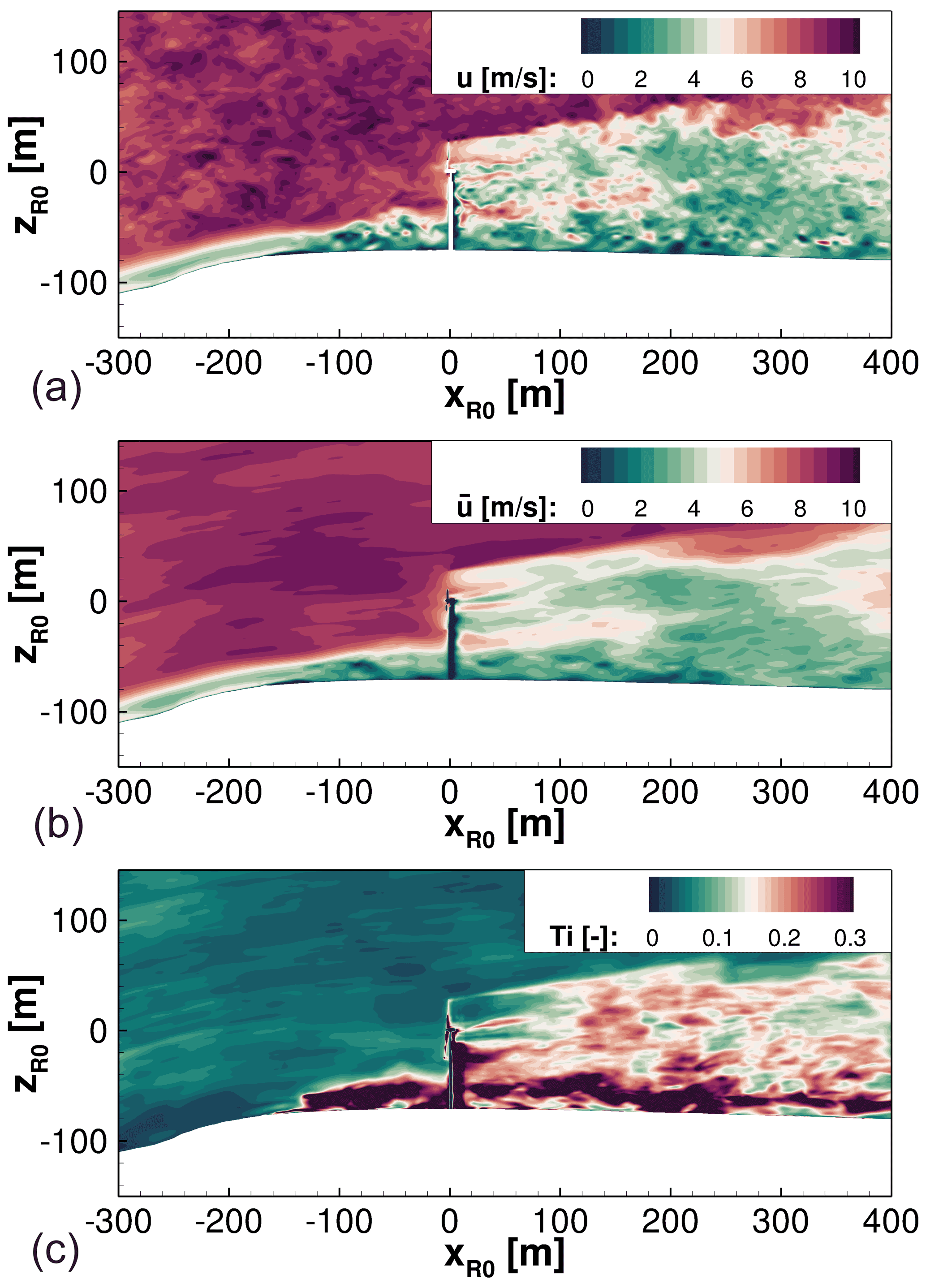
Figure 22 Flow field of a vertical plane crossing the wind turbine position during unstable conditions on 10 March 21. (a) Instantaneous flow field. (b) Averaged flow field. (c) Turbulence intensity of the flow field.

Figure 22 shows a vertical plane of the instantaneous flow field upstream and downstream of the wind turbine.

Despite the lower foliage densities, the unstable conditions lead to significant mixing of the ambient flow with the forest wake, which also affects the inflow on the wind turbine. However, especially the effects on the wake are even stronger. Up to x=200 m downstream of the turbine, the turbine wake is distinguishable from the forest wake. The propagation of the blade tip vortices with increased velocities is also visible in this area. Further downstream the wake structures of the forest and the wind turbine increasingly mix and are subsequently hardly distinguishable from each other. Considering a position that lies even further downstream, a decay of the turbulent wake is noticeable. Temporal averages show similar findings. The middle plot shows such an averaged flow solution over 60 s. The lower plot indicates the turbulence intensity evaluated over the same period. Starting at x=200 m, the wake contour of the turbine mixes with the forest wake to an extent that results in a uniformly spreading wake structure, which rapidly decays. Also, increasing fluctuations arise from the strong mixing of the wind turbine wake and the forest wake. The turbulence production near the ground at $x=-\mathrm{140}$ m downstream of the last tree row is due to transient effects: a combination of temporal flow separations and also moments with high velocities at this position causes these unsteady variations of the wind.

Thus, the high turbulence intensities at these unstable conditions lead to strong fluctuations in the wake. This impact causes the wake to deform when mixing with the forest. The result is a breakdown of the wake further downstream.

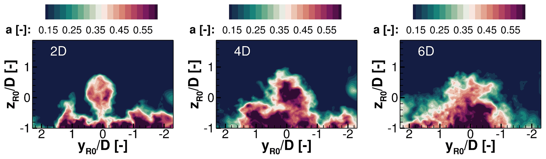
Figure 23 Comparison of the axial induction factors a in transverse planes of the wake 2 D, 4 D, and 6 D downstream of the wind turbine.

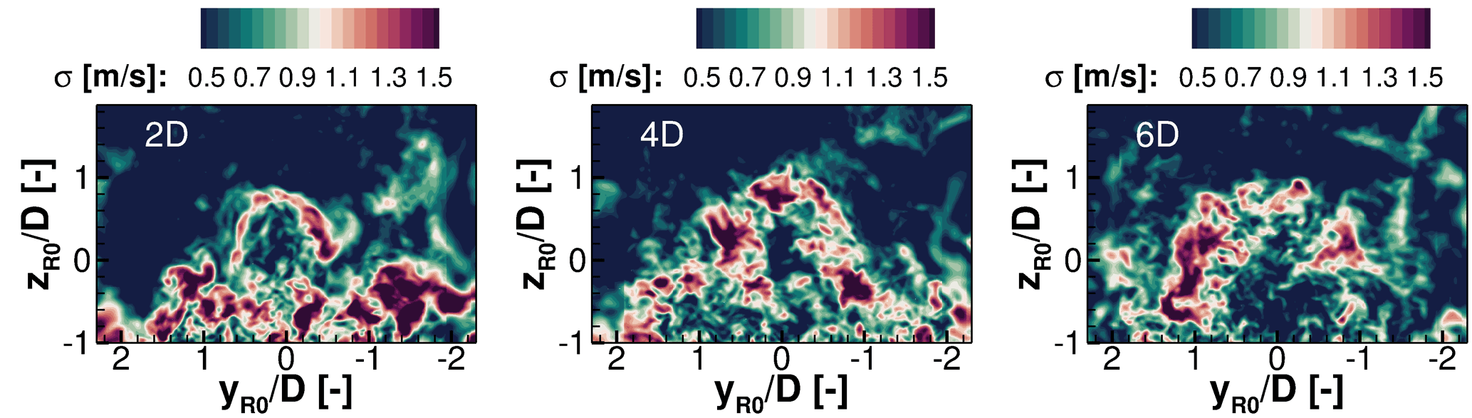
Figure 24 Comparison of the standard deviations σ in transverse planes of the wake 2 D, 4 D, and 6 D downstream of the wind turbine.

The physical behaviour of the flow in the wake will be examined in more detail by looking at transverse planes in Figs. 23 and 24. The planes are extracted 2, 4, and 6 rotor diameters downstream of the turbine, respectively. Figure 23 shows the averaged axial induction factor a to analyse the mean wake propagation. Figure 24 examines the standard deviation σ, which is used to evaluate the decay of the wake with increasing distance. In a distance 2 D downstream of the turbine, by both a and σ, the turbine wake is still distinguishable from the turbulent structures of the forest wake. This means at this position mixing is still relatively low. Two diameters further downstream, a mixing of the wake structures is already visible, and the standard deviation σ depicts that the rotor-induced fluctuations increase and occupy increasingly larger areas. In a distance 6 D downstream of the turbine, forest wake and turbine wake have become a coherent structure. The standard deviation illustrates the decay of the wind turbine wake because the fluctuations propagate into extensive areas.

To analyse the combined topographic and meteorological influences on the wind turbine performance, simulation results examining torque and torque fluctuations are presented below. For this purpose, the results were phase averaged over 25 revolutions.

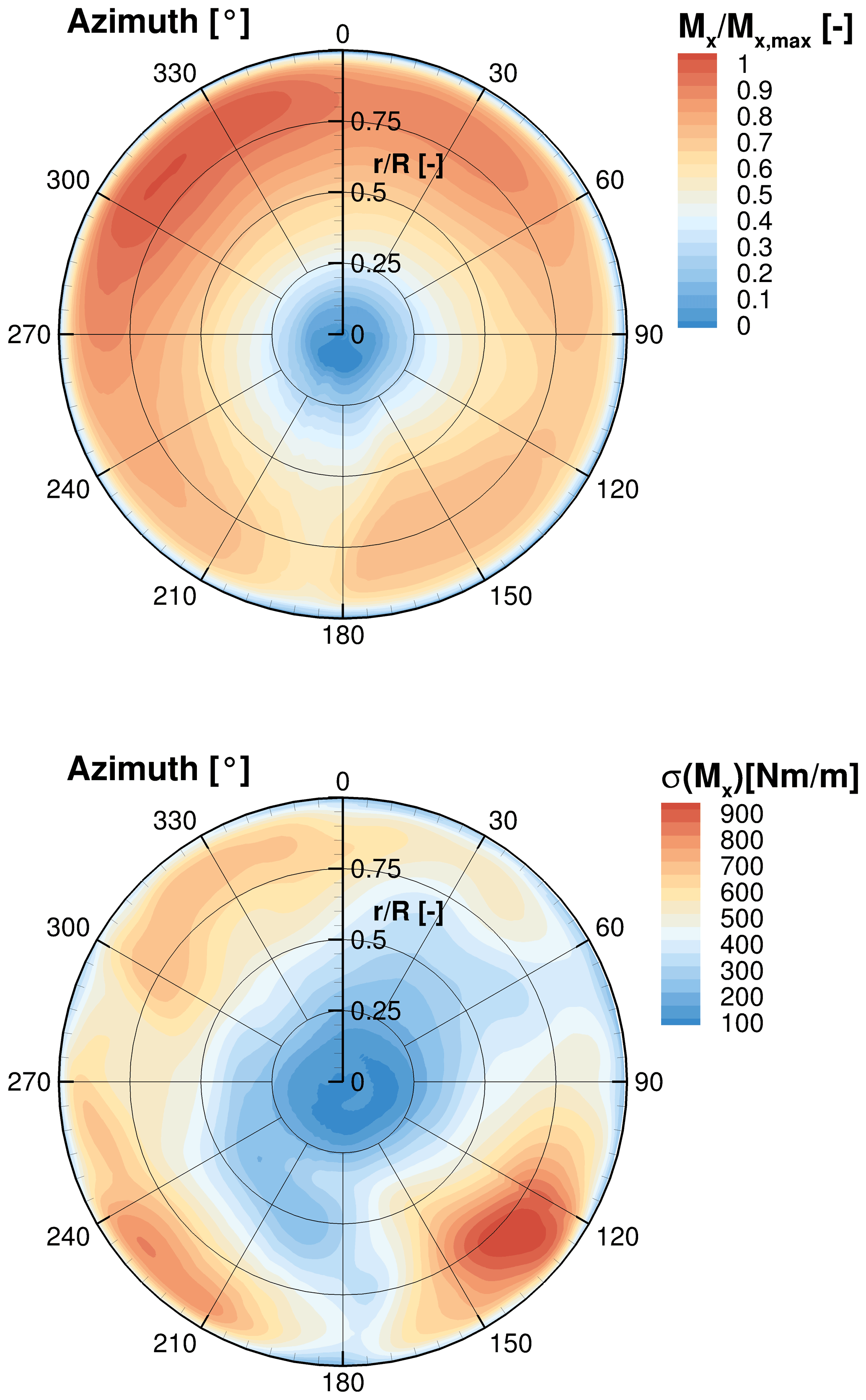
Figure 25 Distributions of the torque and of the standard deviation of the torque phase-averaged over 25 revolutions at the rotor plane.

Figure 25 shows the phase-averaged torque distribution at the rotor plane, which is significantly responsible for generated power of the wind turbine. The upper plot depicts the phase averaged torque normalised by the maximum value. This maximum of the torque is reached in the upper-left area of the rotor plane. The maximum torque is generated between 290 and 340^∘ because of the retreating blade effect. The escarpment of the orography and besides convective conditions with upward-acting buoyancy cause inclined flows. This upward wind increases the angle of attack at this position as the blade retreats in the left rotor half and advances in the right rotor half. The higher angles of attack increase the rotor loads and therefore the torque at this position. The forest wake causes lower torque to be generated in the lower half of the rotor, resulting in a power reduction. As can be interpreted from Fig. 20, the higher torque distributions of the upper rotor plane in contrast to the lower rotor plane do not result from the shear of the velocity profile, as the shear hardly changes over the rotor plane. The differences are rather due to the forest wake and the unstable conditions. At 180^∘ the tower blockage causes lower values of M_x. To gain a better understanding of the effects of the turbulent flow field on the torque, the lower plot shows the standard deviation of the axial torque σ(M_x). The largest torque fluctuations occur in the lower half of the rotor. As already described, turbulent vortices of the forest wake with reduced velocities flow across the lower half of the rotor plane, which leads to temporarily large velocity differences and therefore to high load fluctuations. The maximum of the torque fluctuations is reached between azimuth positions 120 and 150^∘. In this area the highest turbulent fluctuations occur as already analysed in the lower plot of Fig. 21. The increased load fluctuations arise across the entire lower half of the rotor. Because of the tower passage of the blade and the associated tower blockage, smaller torque fluctuations occur at 180^∘. Increased torque fluctuations also occur at the areas of the maximum rotor loads between 290 and 340^∘. The high ambient turbulence causes gusts that affect the inflow for this rotor position in the observed period.

Many conditions affect the wind turbine at the test site. The orography leads to accelerations above the escarpment. The forest induces reduced velocities close to the ground, resulting in large shear effects and amplified turbulence. In addition, high turbulence intensities induced by the orography and convective flows have a strong impact on the wind turbine.

5 Conclusions

The paper presents the results of a study of highly resolved DDESs of a wind energy test site in complex terrain that is currently under construction in southern Germany. In the first part of the results, the effects resulting from orography, forests, and thermal stratification were investigated and evaluated separately. Initially, the effects on the flow field were analysed, and in a second step, the fully meshed wind turbine was integrated into the flow field. Subsequently, all effects were combined and applied to a study with real observed conditions on 10 March 2021 in the second part of the results. The results of the simulated flow field were compared with met mast data. For the evaluation of this work, only comparative measurements of the wind field were available, as the construction of the turbines had not yet been completed on the test field at that time. Numerically, however, the wind turbine could be considered for this period, which was subsequently also done in the results. The inflow, the wake, and the performance output of the wind turbine were investigated. The main findings are listed below.

1. The escarpment accelerates the flow field at the altitude of the rotor plane. The analyses of the flow field showed that in the investigated terrain on the Swabian Alps, speed-ups of 35 % to approximately 60 % result at hub height compared to the velocities in the valley at the same reference height. In combination with the upper flow field that is less influenced by the orography, a boundary layer profile with low shear versus altitude results on the plateau of the wind energy test site.

2. At the test site, the forest has a large impact on the flow field in ground proximity. The numerical studies showed that the forest wake can spread up to heights of 60 m approximately 200 m downstream of the last row of trees on the escarpment where the wind turbine is located in the simulations. The horizontal wind speed also has an impact on the spread of the forest wake. The higher the horizontal speed, the higher the acceleration of the vertical speed over the steep slope. Accordingly, the forest wake spreads to larger heights. In some cases, these turbulent wake structures also reach hub height. Highly turbulent fluctuations of low wind speeds in the forest wake strongly mix with the high-velocity flow field above and result in highly complex and turbulent flow situations. For a reference wind speed at hub height of 11 m s⁻¹, the standard deviation at the turbine position can reach approximately σ=3 m s⁻¹, which corresponds to extremely high turbulence intensities due to the low average wind speeds near the ground in the forest wake. For a reference wind speed at hub height of approximately 7.7 m s⁻¹ and lower leaf area densities, the standard deviation can still be σ=1.5 m s⁻¹ to σ=2 m s⁻¹, which dominates the flow near the ground.

3. Thermal stratification also has a strong impact on the ambient turbulence and the forest wake. Stable conditions suppress turbulent mixing, especially downstream of the forested escarpment, whereas turbulence is strongly amplified for convective conditions. The height differences of the forest wake between stable and unstable stratification at the turbine position as analysed in this work can reach approximately 25 m, which can influence the rotor loads, the power, and also the wake very differently.

4. By considering the wind turbine in the flow field, it has been shown that the forested escarpment impacts the inflow of the turbine, as well as the mixing of the forest wake with the turbine wake. This affects wake decay further downstream. Unstable conditions amplify this effect, while in stable conditions the wake extends further downstream. In unstable conditions 6 D downstream of the turbine, the turbulent wake spreads laterally and vertically in approximately 30 % larger areas than for stable conditions.

5. Taking all these effects into account when simulating real conditions of a 5 min period on 10 March 2021, decent agreements with the mean velocity profile and the turbulent statistics measured by the met masts were shown. The deviation of all measurement points of the velocity profile to the simulated results remains in a range of ±1 m s⁻¹. In most cases, the deviations of the measured and simulated values in the range relevant for the wind turbine are even significantly smaller. A similar statement is also valid for the comparison of the standard deviation. Especially in the lower area below the hub height, which is strongly influenced by the very turbulent forest wake, there are very good agreements with the measured data. The deviations $\mathrm{\Delta }\mathit{\sigma }=|{\mathit{\sigma }}_{\mathrm{mesured}}-{\mathit{\sigma }}_{\mathrm{simulated}}|$ are generally less than Δσ≈0.3 m s⁻¹ (<25 % deviation).

6. The prevailing unstable conditions led to increased mixing of the ambient turbulent flow with the forest wake. This had an increased effect on the inflow of the rotor plane and on turbulence amplification in the forest wake.

7. To evaluate the performance output of a virtual turbine, all of these effects had to be considered. Topographic effects and convective conditions cause low shear at the rotor position on the plateau. However, vortex structures that detach from the forest occasionally cross the rotor plane and have a significant impact on performance in the lower half of the rotor. Inclined flows in the escarpment are intensified by convective conditions, resulting in increasing angles of attack and, therefore, more torque in the left rotor plane. The highly turbulent flow in the test field also impacts the turbine rotor strongly. The simulation analyses of the influences on the rotor loads have shown that many factors can have a great impact on the performance of the wind turbine and lead to very heterogeneous load cycles. These load cycles analysed here are hardly predictable for simplified tools. It was also shown that despite the large turbulent fluctuations, the wind speed increase due to escarpment can be profitably used for wind energy. In particular, the AEP will be higher at the test site compared to a location in the valley, which makes this wind energy site profitable.

This paper emphasised the importance of considering orography, vegetation, and thermal stratification in numerical simulations to resolve the flow field decently. In this way, the effects on inflow, loads, power, and wake of the wind turbine can also be predicted well.