the Creative Commons Attribution 4.0 License.
the Creative Commons Attribution 4.0 License.
 | 30 Aug 2022
High-Reynolds-number wind turbine blade equipped with root spoilers – Part 2: Impact on energy production and turbine lifetime
Thomas Potentier
Emmanuel Guilmineau
Arthur Finez
Colin Le Bourdat
Caroline Braud
A wind turbine blade equipped with root spoilers is analysed using time domain aeroelastic blade element momentum (BEM) simulations to assess the impact of passive devices on the turbine annual energy production (AEP) and lifetime. Previous 2D computational fluid dynamics (CFD) showed a large unsteadiness in aerodynamic coefficients associated with the spoiler, and such behaviour is captured by the OpenFAST simulations when all degrees of freedom are switched off. Once the turbine is fully flexible, a novel way to account for aerofoil-generated unsteadiness in the fatigue calculation is proposed and detailed. The outcome shows that spoilers, on average, can increase the AEP of the turbine. However, the structural impacts on the turbine can be severe if not accounted for initially in the turbine design.
- Article
(6360 KB) - Full-text XML
- BibTeX
- EndNote


Thanks to a steady rotor size increase over the last decades, the wind energy sector managed to grow. In the onshore wind sector, due to various limitations, the rotor diameter remains constrained, but blades over 60 m long are now common. Larger blades require more attention to detail during the design phase to reduce the cost. The maintenance cost during the turbine lifetime increases too, and a good understanding of the turbine ageing is necessary.
In order to reduce the levellized cost of energy (LCOE), turbine manufacturers had to imagine solutions to increase the energy output of existing turbines. Among such solutions, there are aerodynamic add-ons (AAOs), which are mostly passive devices attached to the blade surface to either lower the acoustic emission or increase the power extraction locally.
With the increasing rotor diameter and hub height, turbine manufacturers are now facing aeroelastic challenges where tower and blades can deform over large distances. Before several extensive measurement campaigns of scaled models in large wind tunnels or in the field were performed (see Hand et al., 2001; Simms et al., 2001; Snel et al., 2007; Boorsma and Schepers, 2014; Madsen et al., 2010; Trodborg et al., 2013), the physical phenomenon of wind loading unsteadiness was poorly understood and large safety factors were used to ensure the turbine robustness and design lifetime. High-fidelity tools such as computational fluid dynamics (CFD) could perform that task, but the computational cost would render the turbine's time to market too important. In another hand, turbine designers using quicker engineering tools such as blade element momentum (BEM) lacked, at first, the necessary unsteady models. Now, it is common knowledge to be using unsteady models to simulate wind turbines, and it is referenced in many textbooks (Hansen, 2015; Burton, 2001). The large-scale unsteadiness investigated showed that the atmospheric boundary layer, turbulent wind, yawed inflow or even blade pitching can have a serious impact on the turbine if not properly accounted for, as found in Potentier et al. (2021). One of the remaining challenges to predict the turbine loads even more accurately is to account for the local unsteadiness, self generated by the flow travelling around an aerofoil, which can interact with large-scale unsteadiness. As detailed in Potentier et al. (2022), where thick blade profiles equipped with blade root AAO were studied with 2D CFD with low-turbulence-intensity free-stream conditions, the spoiler produces the desired higher lift by reorganizing the flow and pressure distribution around the aerofoil. In consequence the unsteady behaviour (vortex shedding) behind the aerofoil is vastly different from the bare blade.
ENGIE Green is a French exploiting party of renewable energy sources. During routine maintenance, some cracks have been noted at the blade root near the spoiler installation. The present paper aims at understanding the aerodynamic causes of the structural failure, using state-of-the-art calculation methods and proposing a novel way of predicting the impact of spoiler on the blade structure lifetime. The AEP gain will also be evaluated. Because performing fatigue calculation using CFD would be too computationally expensive, and BEM cannot directly account for aerodynamic unsteadiness, in this paper we propose bridging the gap by utilizing the strengths of both simulation methods. First the methodology to build the aeroelastic model is explained in Sect. 2. The use of 2D CFD associated with aeroelastic BEM simulation will allow us to compare between the two configurations the aerodynamic parameters such as lift coefficient (CL), axial induction (a), rotor loads, power and energy production (Sect. 3.1). A novel way of accounting for polar unsteadiness in the fatigue lifetime calculation is proposed in Section 3.2. A validation using 3D CFD, for a single wind speed, is currently being done to assess the vortex shedding behaviour on the rotor.
2.1 Wind turbine blade and aerofoil shape
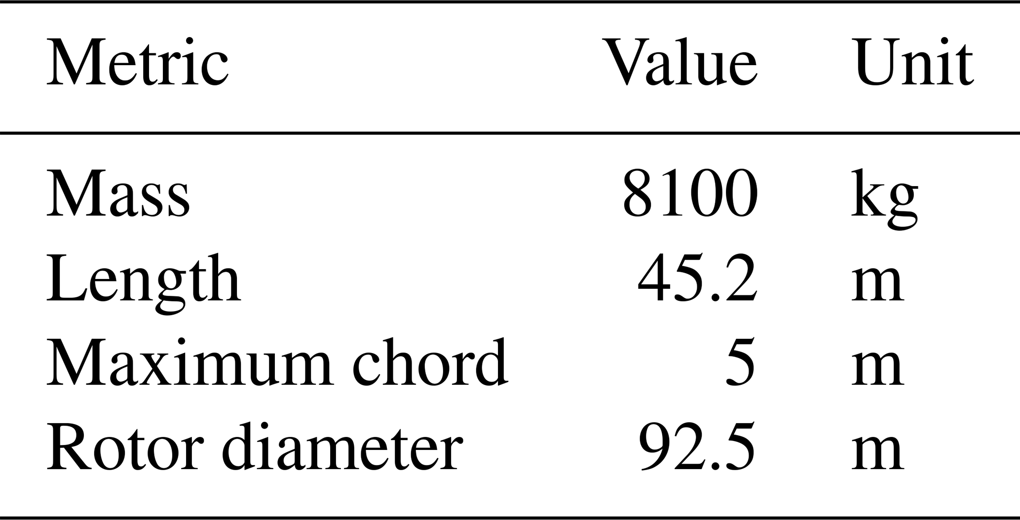
The wind turbine geometry used in the present study was acquired during a scanning campaign on an operating 2 MW turbine (see Dambrine, 2010); the rotor diameter is 92 m and the maximum height reach is 150 m above ground. During the scan post-treatment the chord, twist and thickness were also extracted, defining the blade geometry (see Fig. 2). One can note the typical “de-twist” toward the blade tip to alleviate the blade loading. The blade geometry is discretized more densely at the root of the blade since the spoiler is installed at this location. More details about the scan post-treatment are available in Potentier et al. (2022). The scanned blade was originally equipped with root spoilers. The blade without spoiler was generated by manually removing parts of the cloud points corresponding to the spoiler location; consequently wherever the spoiler is not present both aerofoils geometries are identical (see Fig. 1). For the rest of the study, the simulations will take place on the real scale, i.e. using the scan outputs as blade geometry.
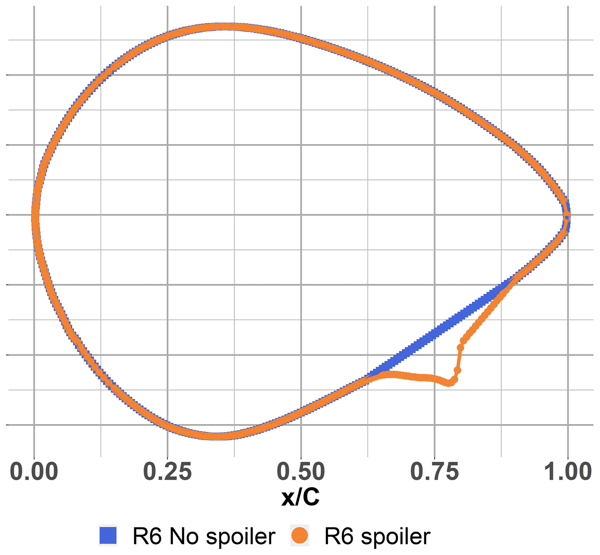
Figure 1Overimposed aerofoil shapes at radial position R6 ( %): the blue square (blue ▪) shows the no-spoiler coordinates while the orange dot (orange •) shows the spoiler coordinates.
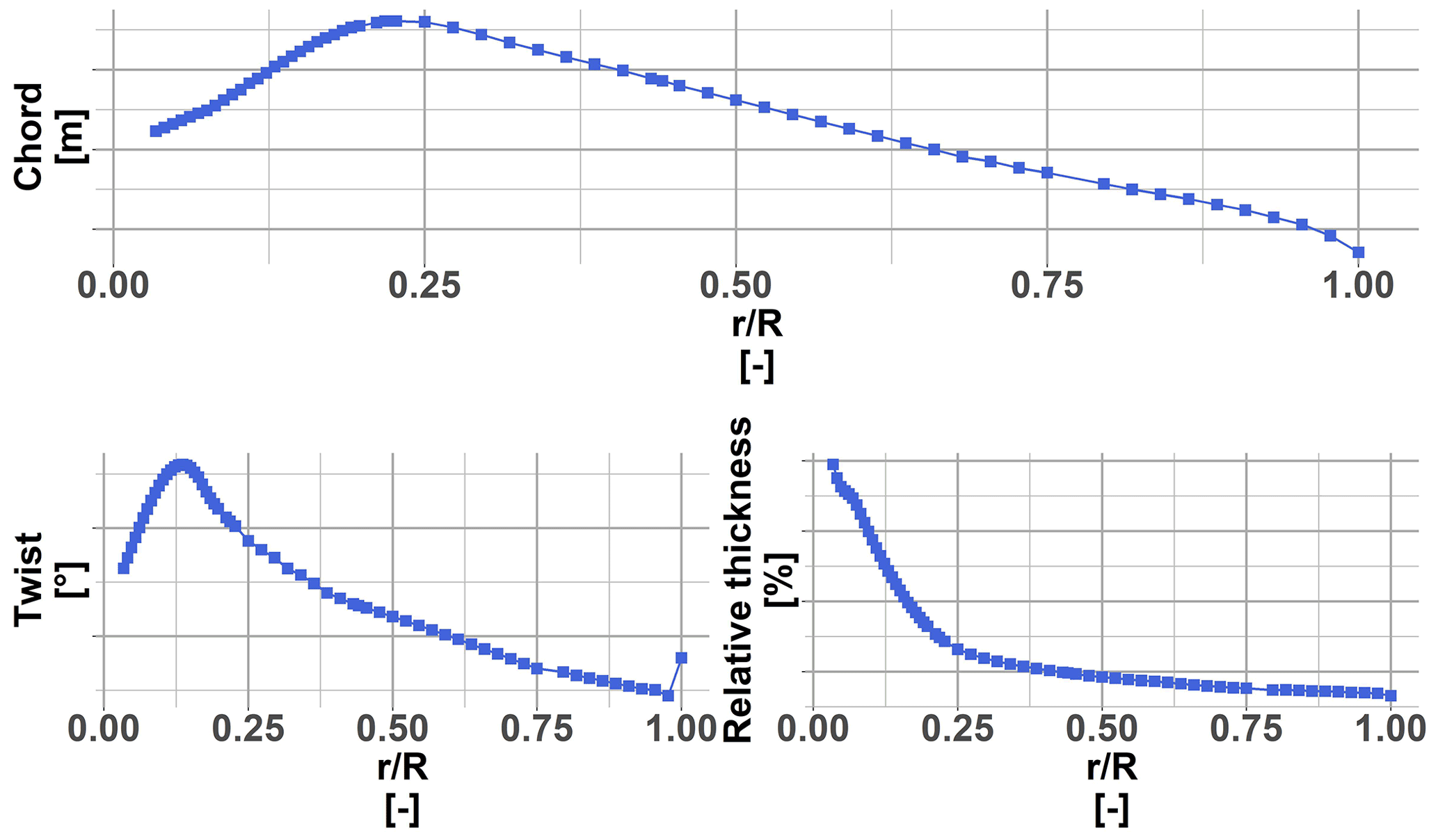
Figure 2The scanned blade geometry: chord, twist and relative thickness distribution against the normalized radius.
2.2 Unsteady aerodynamic BEM inputs
The tools used to perform the spoiler impact assessment are CFD for the polar generation and blade element momentum (BEM) theory for the aerodynamic calculations. BEM is used to calculate associated loads and compute the turbine annual energy production (AEP). The BEM solver used is the AeroDyn module (see Jonkman et al., 2015) from OpenFAST (https://openfast.readthedocs.io/en/main/ website, last access: 8 November 2021). OpenFAST can produce a large variety of sensors, which are calculated outputs during the simulation.
AeroDyn is a well-known tool developed by NREL and has been used in many international or academic projects. A thorough explanation of the BEM theory is available in textbooks such as Hansen (2015) or Burton (2001). A brief step-by-step approach written below summarizes the iterative BEM procedure.
-
The axial induction factor a and the tangential induction factor a′ are first estimated (typically ) only during the first loop. For the following loops the induction values used are those from the previous iteration (see step 7).
-
Then, the inflow angle φ is estimated from the instantaneous velocity inflow Vw, the rotor rotational speed ω and the local radius r.
-
The angle of attack, α, is computed using the blade element theory (BET) with θ the local twist angle and β the blade pitch angle.
-
Read the CL, CD (drag coefficient) and CM (moment coefficient around the one-fourth chord position) from the polar associated with the analysed radius.
-
Calculate the loads in the rotor plane using CL, CD and φ.
-
To account for the finite blade span, the Prandtl tip correction factor is calculated.
-
The initial induction coefficients, a and a′, are updated accounting for highly loaded rotors.
-
The unsteady BEM equations can be applied: yaw models, dynamic wake model, blade acceleration due to its deflection and tower shadow effect.
-
A convergence criterion, ϵ, is defined, and the iteration process restarts from step 2, using the updated induction values, until the convergence criterion is reached.
-
After convergence, the local loads (aerofoil level) can be calculated.
-
Once all elements are converged, the integrated loads (rotor and turbine level) can be computed.
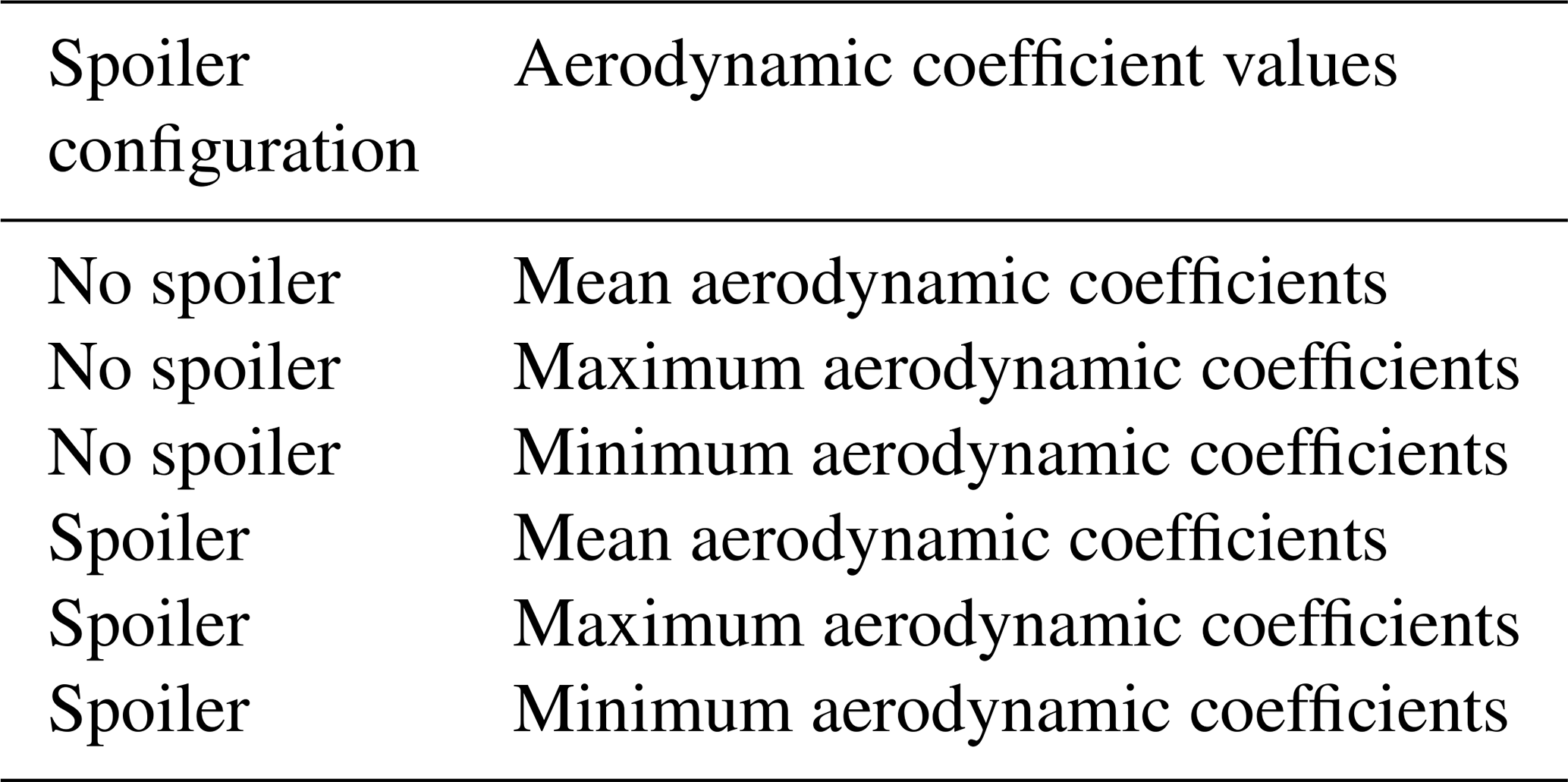
The procedure described relies on steady polar to perform the iterative steps; it is an inherent BEM limitation. However, as highlighted in Potentier et al. (2022), aerodynamic properties become highly unsteady at the blade root when a spoiler is present. To overcome the single steady polar limitation and use the unsteady coefficient, we decided to generate three steady polars corresponding to the mean, minimum and maximum CL, CD and CM for each turbine case: “no spoiler” and “spoiler” (see Table 1). Those mean, minimum and maximum coefficients are representative of the states reached by the aerodynamic coefficients during the time series calculated using 2D CFD as found in Potentier et al. (2022) (see e.g. Fig. 3).
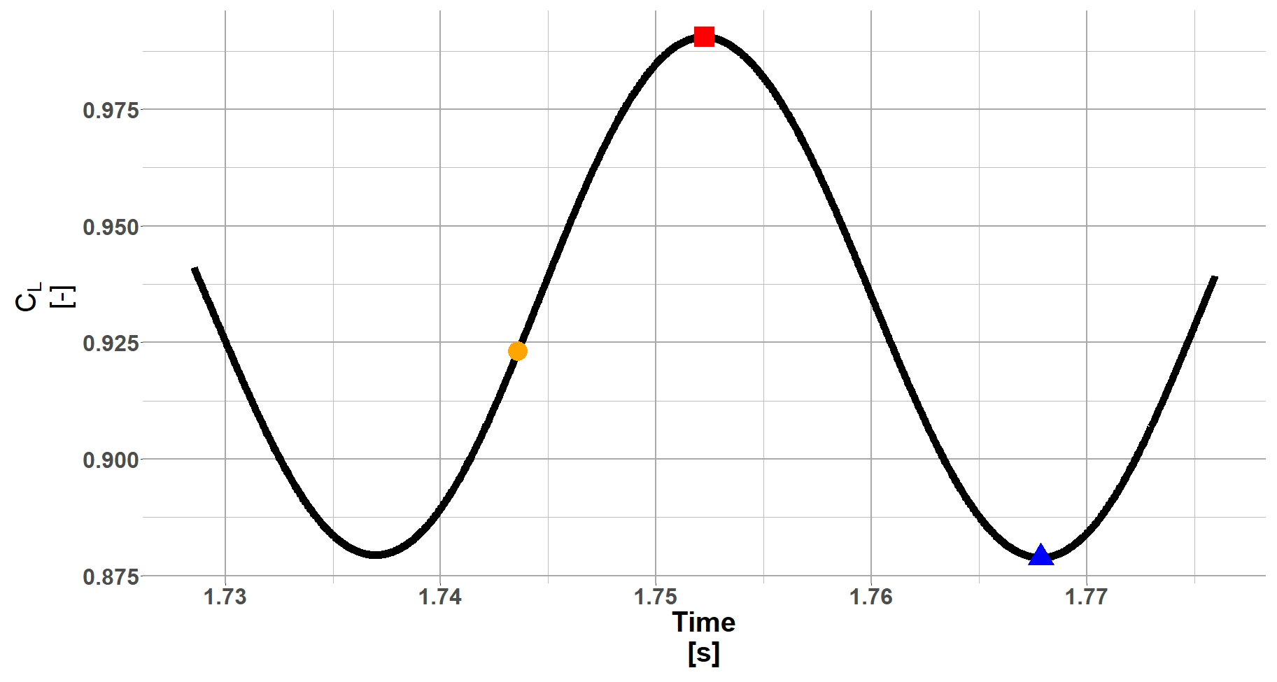
Figure 3Spoiler case CL evolution in time α=6∘ and . The blue triangle (blue ▴) corresponds to the minimum CL, the red square (red ▪) corresponds to the maximum CL and the orange dot (orange •) corresponds to the mean CL.
2.3 Turbine structure scaling
The scan does not give any information on the blade's material, since only the outer skin was measured. Material properties are a crucial element for turbine design, and as part of an academic or wind turbine exploiting party, we do not have access to this information. Therefore, for the rest of the aeroelastic study, the blade and tower mechanical properties will be scaled using the open-source NREL 5 MW turbine (see Jonkman et al., 2009). Some hypotheses and assumptions had to be made and will be explained below. Usually, scaling is made to reach the same level of stress or reach similarity in physical phenomena: Mach number, Reynolds number and Froude number (see Campagnolo, 2013). Here, since the stress target values are unknown and the physics similarity is already achieved (Mach, Reynolds and Froude numbers close enough between the NREL turbine and the ENGIE Green turbine), we decided to scale the turbine based on geometric properties. The NREL turbine has a 63 m long blade and its tower is 87.6 m high. In comparison the ENGIE Green turbine has a blade length of 45 m and the tower height is 80 m. Several scaling procedures exist and have been described in Loth et al. (2017) and Canet et al. (2021). The authors aimed at creating a sub-scale model for wind tunnel or field testing, where the difference between both models is large (reduction factor up to 90). In our case, we desired to use known mechanical properties and adjust them based on the smaller blade and tower length, so that the ENGIE Green turbine behaves similarly to the NREL one. Therefore, the method used varies slightly compared to the literature and is described below.
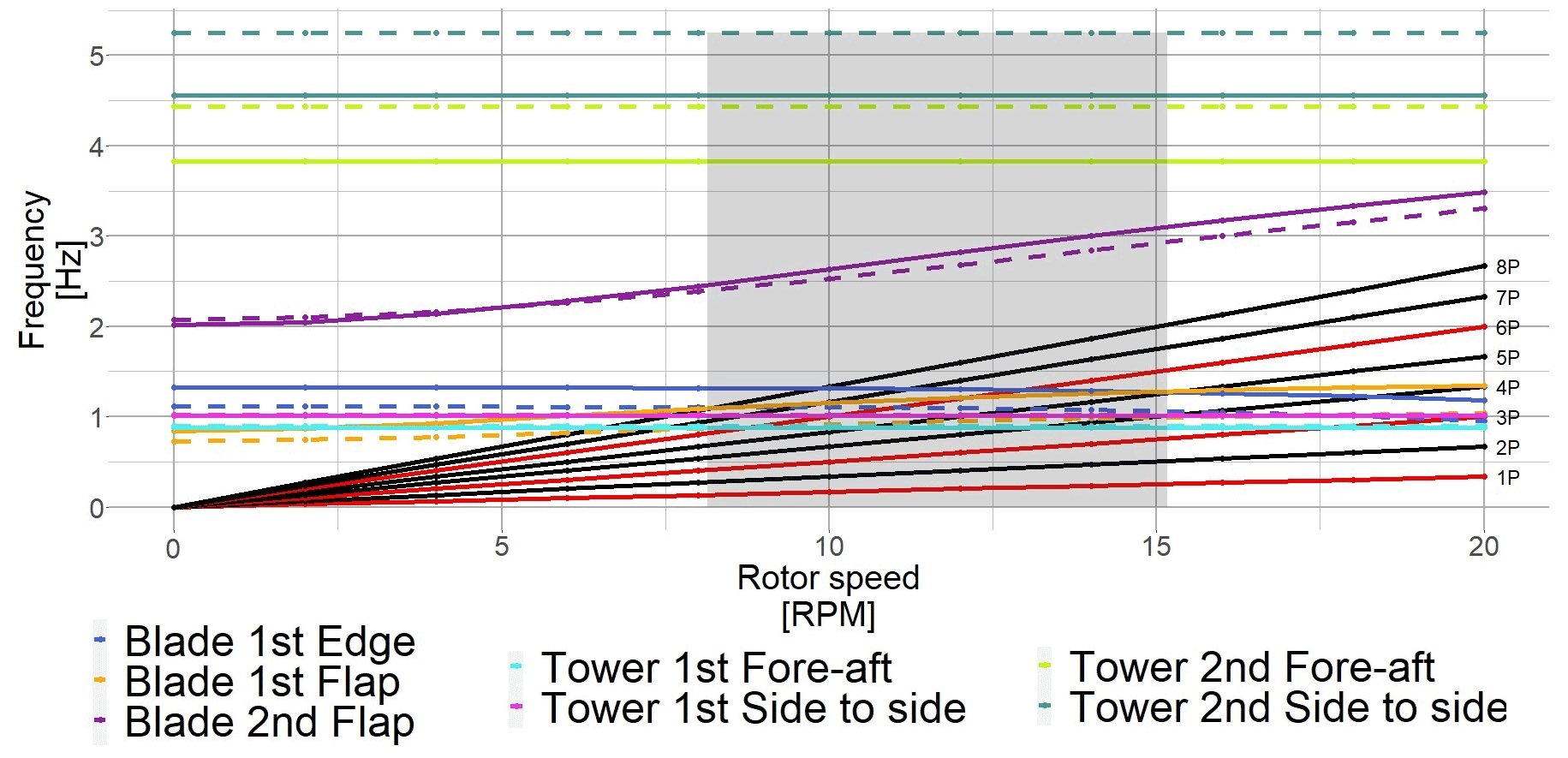
Figure 4Campbell diagram comparison between the NREL reference turbine and the ENGIE Green scaled one. The solid lines show the NREL response, and the dashed lines show the ENGIE Green turbine's response. The dark shaded area illustrates the ENGIE Green's turbine range of operation.
The blade structural properties needed are the edgewise and flapwise local stiffnesses along the radius: EIxx and EIyy, as well as the linear mass ML. E is the Young modulus while Ixx and Iyy are respectively the in-plane and out-of-plane sectional moment of inertia. Assuming identical material is used to manufacture both blades, only the sectional inertiae Ixx and Iyy vary. Since the sectional inertia varies based on geometric properties, we decided to use the chord as the main driver for the change in properties. The thickness could also have been chosen, but the chord was preferred because of its larger absolute value. Also, the edgewise stiffness could have been scaled based on the chord thickness and thickness for the flapwise stiffness. It was decided to only use the chord as a basis for the scaling for simplicity. Further studies could be done to assess the validity of the assumption. In our geometric scaling we multiply the NREL 5 MW stiffnesses EIxx and EIyy by the ratio of the local chord along the radius to the power of 4 (see Eq. 1), thanks to dimensional analysis. Following the same reasoning, we assume an identical material, and the NREL 5 MW linear mass needs to be multiplied by the chord ratio at the power of 1 (see Eq. 2). The same methodology is applied to the tower stiffnesses and mass.
Here, E is the material Young modulus, and are the ENGIE Green blade local inertiae, and and are the NREL's 5 MW turbine initial local inertiae. and are the NREL's 5 MW and ENGIE Green's blade chords at the same spanwise location, and the subscript j shows the analysed station.
where and are the linear mass of both blades and the subscript j shows the analysed station.
Moreover, the blade and tower modal shapes, necessary OpenFAST inputs, have been recalculated using the scaled mechanical properties. A Campbell diagram illustrates that despite the difference in length and mass, both turbines behave similarly, as desired (see Fig. 4). All ENGIE Green blade modes follow the NREL baseline turbine trend with a little offset due to the shorter blade. Regarding the tower, the first modes (fore–aft and side-to-side) are identical between both turbines; only the second modes show a clear offset towards the highest frequencies.
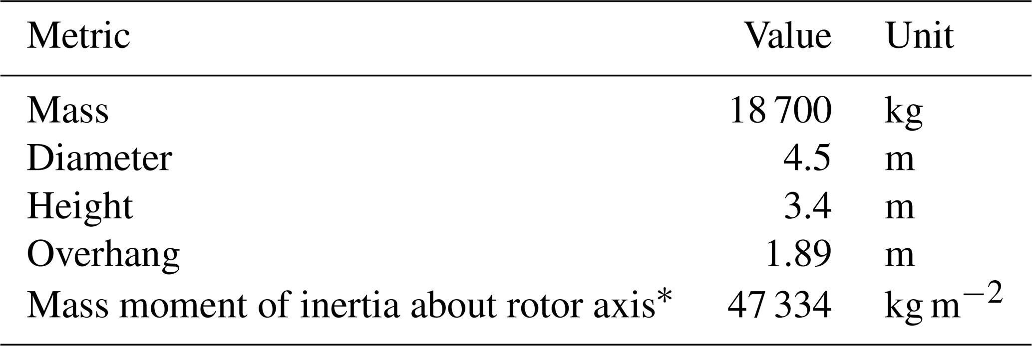
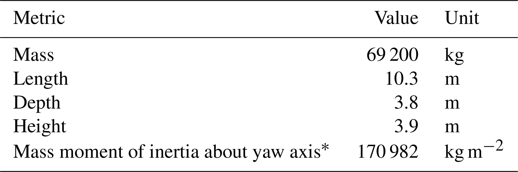
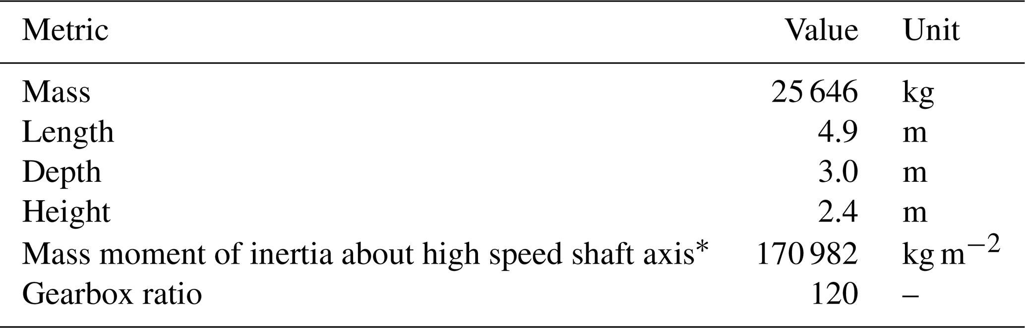
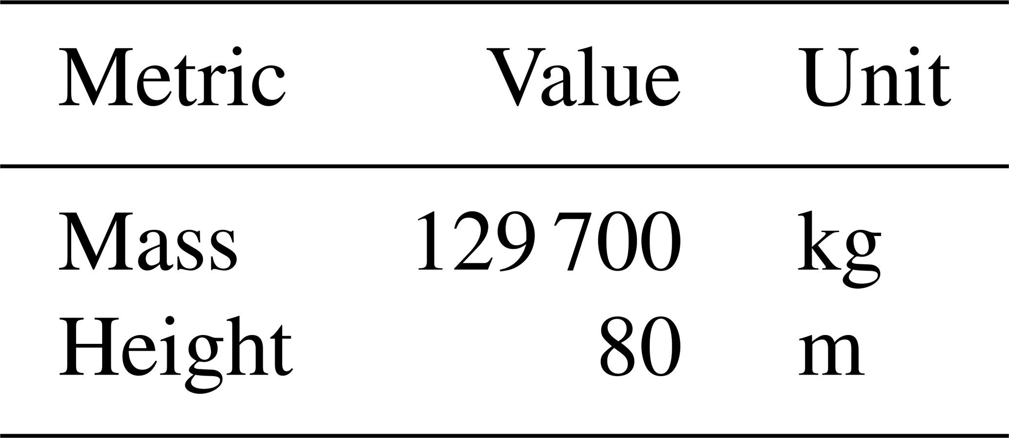
A final sanity check was performed on the mass to assess the validity of the scaling. The blade and tower mass where respectively 0.6 % and 1.3 % off compared to the manufacturer's design specifications, which is small enough to be acceptable. Figures 5 and 6 show the mechanical property comparison with the original NREL 5 MW turbine. Finally, the turbine characteristics publicly available and necessary for OpenFAST are gathered (see Appendix A).

Figure 5Blade stiffness properties. The blue lines (blue −) show the scaled blade and the orange lines (orange −) the original NREL 5 MW blade properties. The symbols ▪ and ▴ show the different stiffness directions.
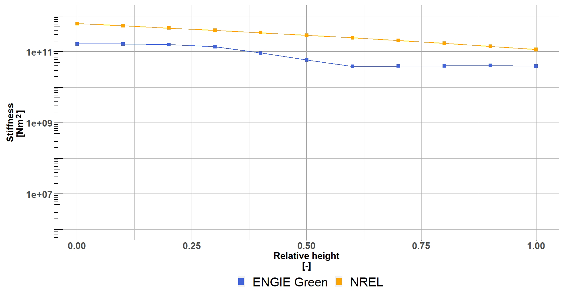
Figure 6Tower stiffness properties. The blue lines (blue −) show the scaled tower and the orange lines (orange −) the original NREL 5 MW tower properties. Because fore–aft and side-to-side stiffnesses are identical only a single curve per tower is shown.
2.4 Unsteady polar generation
The grid independence study and polar generation methodology have already been performed and presented in Potentier et al. (2022). Then, all 16 profiles listed in Table 2 were computed to extract aerofoil aerodynamic coefficients (lift, drag and moment coefficients) for OpenFAST computations. Thus producing six different steady polars for the turbine (see Table 1). Figures 7 and 8 show representative sections for the lift and drag coefficient along the blade span. The solid lines show the mean aerodynamic coefficient values, while the shaded areas illustrate the range of variation reached during each angle of attack calculation. Consequently, the polar using the maximum aerodynamic coefficients corresponds to the upper limit, and the polar using the minimum aerodynamic coefficient follows the lower limit.
Table 2CFD-calculated blade section polars defining the BEM model assuming an inflow between 8 and 8.5 m s−1.
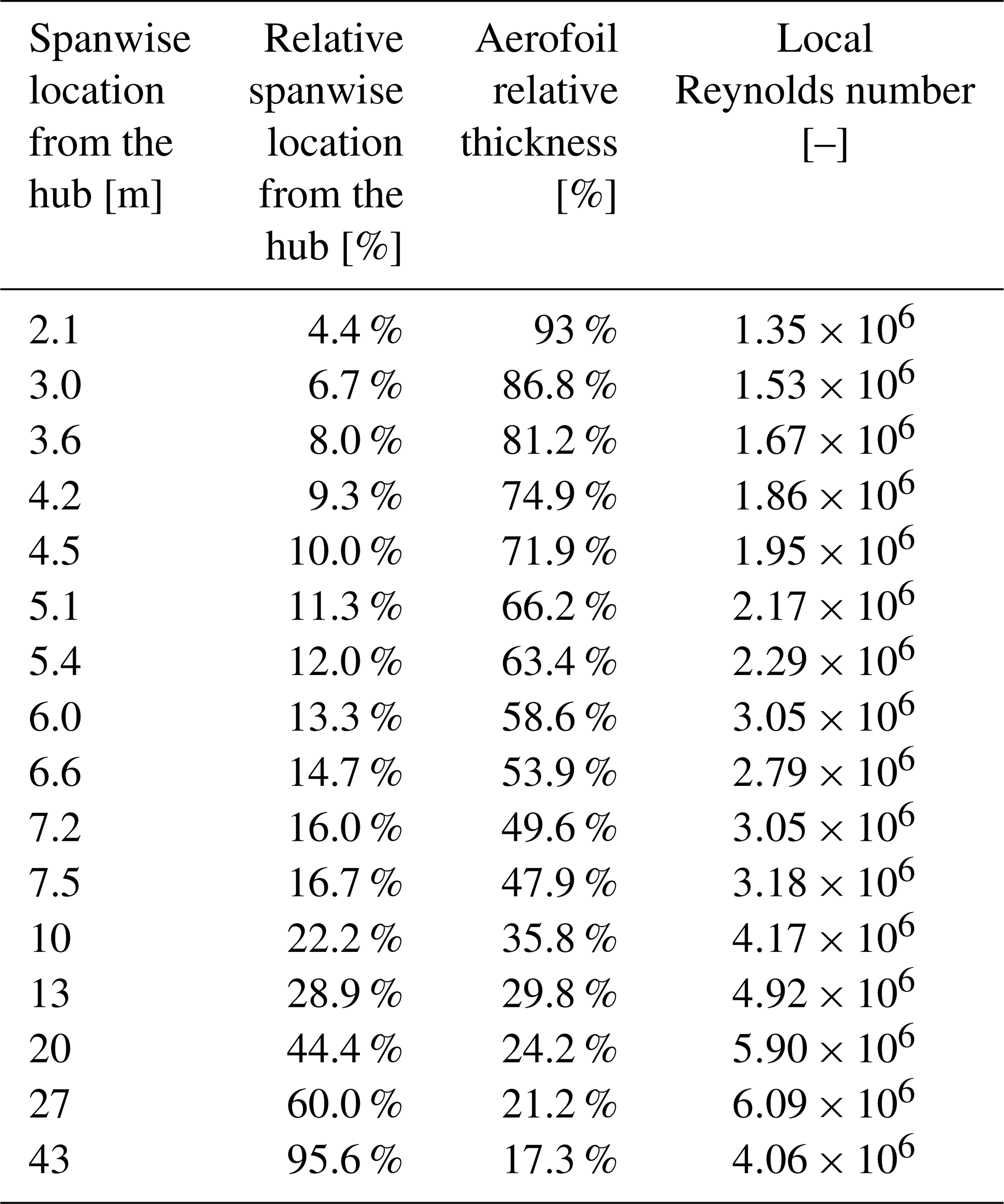
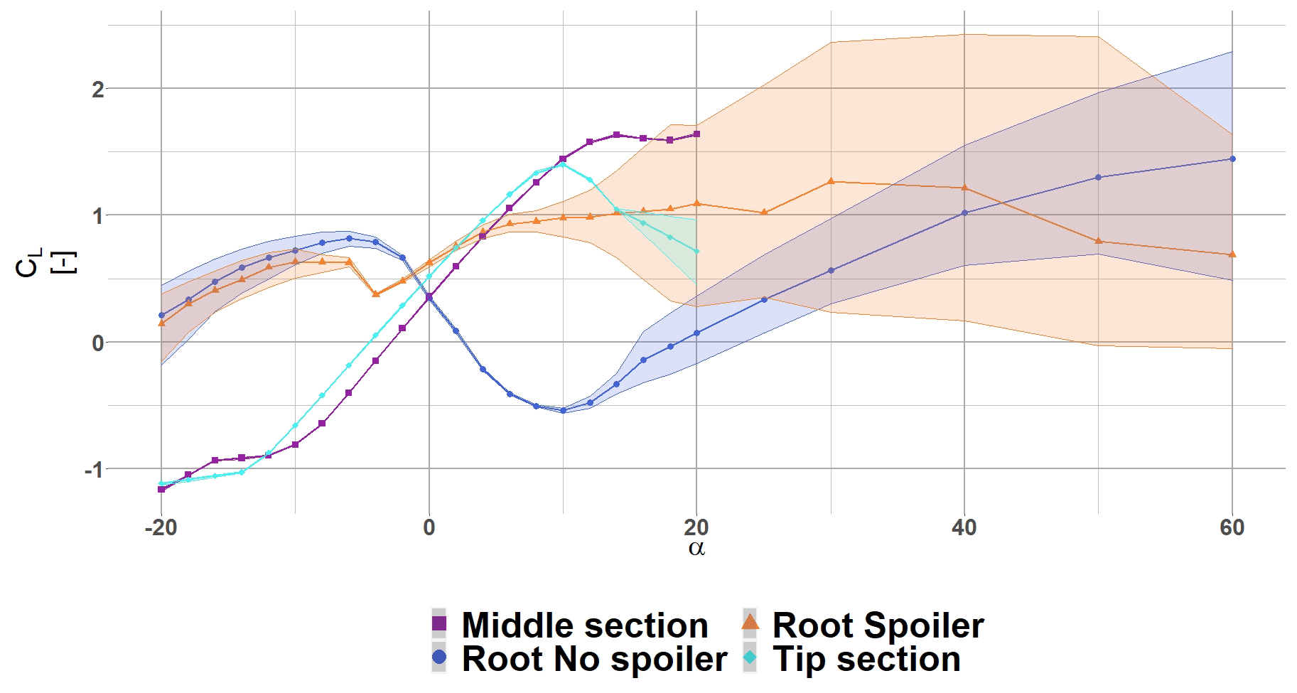
Figure 7The blue dot (blue •) shows the CL for a representative root section without spoiler, the orange triangle (orange ▴) shows the CL for a representative root section with spoiler, the purple square (violet ▪) shows the CL for a representative middle section and the cyan diamond (cyan ⧫) shows the CL for a representative tip section. The shaded areas illustrate the range of variation (maximum and minimum) reached during each angle of attack calculation. The plotted polars have not been corrected with a rotational model.
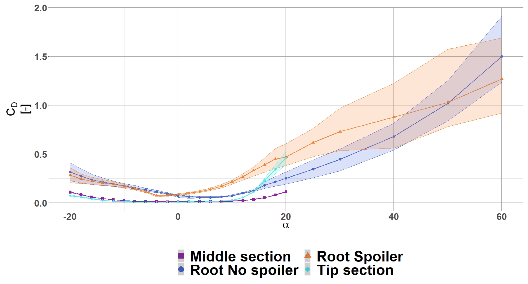
Figure 8The blue dot (blue •) shows the CD for a representative root section without spoiler, the orange triangle (orange ▴) shows the CD for a representative root section with spoiler, the purple square (violet ▪) shows the CD for a representative middle section and the cyan diamond (cyan ⧫) shows the CD for a representative tip section. The shaded areas illustrate the range of variation (maximum and minimum) reached during each angle of attack calculation. The plotted polars have not been corrected with a rotational model.
Initial BEM simulations showed that high angles of attack can be reached (α>50∘) for the inner sections; for this reason the inboard section polars have been simulated up to α=60∘. Each polar has then been extrapolated using the Viterna extrapolation method from Viterna and Janetzke (1982) to cover the full 360∘ range (). Then, to account for the rotational effects, the 3D correction model derived by Chaviaropoulos was used (see Chaviaropoulos and Hansen, 2000).
2.5 BEM simulation set-up
The following sections will detail the model set-up used during the aeroelastic simulations. The first goal of the present paper is to determine the maximum aerodynamic potential of spoilers compared to a bare blade, free of any constraints. A second goal is to assess the impact of the spoiler, on the turbine lifetime, when running at maximum power extraction.
2.5.1 Pitch settings for maximal power production
The pitch settings for maximum power extraction are unknown. The turbine manufacturers may not recommend maximum power generation pitch settings due to potential noise, stall or load issues. Therefore, using SCADA measurements is not sufficient, and an optimization study is necessary. In order to reduce the optimization space to only a single variable (the pitch settings), we assume that the turbine's rotational speed available thanks to averaged field measurements is optimized and will not vary. Then, a search for the optimum pitch settings was carried out for each wind speed between cut-in (3 m s−1) and cut-out (20 m s−1), by increments of 0.5 m s−1, and for each turbine configuration (see Table 1). The optimization constraints are described as follows: below rated wind speed (here 10.5 m s−1), the power production has to be maximal, whilst from rated wind speed until cut-out the turbine must regulate the generated power in order to maintain rated power (here 2.05 MW). A sweep of pitch settings for a range between −10 and 10∘ below rated and between 0 and 20∘ above rated was tried. Figure 9 shows the outcome of the trials for the turbine with spoiler using the mean aerodynamic coefficient polar: the response surface of the optimization procedure. The black line shows the optimal pitch settings for maximal power production. Table 3 shows that the blade with spoiler needs a higher pitch to achieve rated power, thus reducing the angle of attack. Figure 10 shows the outcome of the study for all configurations tested. As can be seen, the difference between both the no spoiler and spoiler is small.
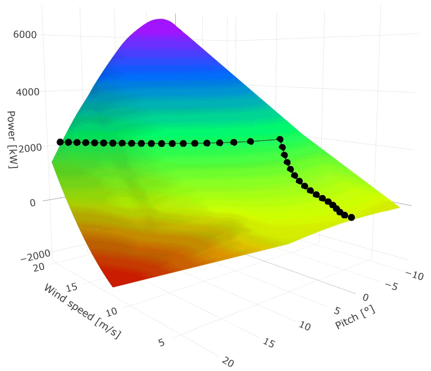
Figure 9Power surface response with varying pitch settings for different wind speeds for the spoiler case using mean aerodynamic polar. The black dotted line is the turbine's optimal pitch settings for maximum power generation.
Table 3Optimal pitch settings for both no spoiler and spoiler cases using mean aerodynamic polars.


Figure 10The blue square (blue ▪) shows the pitch evolution with respect to the wind speed without spoiler, and the orange dot (orange •) shows the pitch with respect to the wind speed with spoiler.
2.5.2 Rigid turbine simulations
In the first analysis, the turbine is considered rigid (i.e. not flexible) with the hub height 80 m above ground using the standalone AeroDyn module. The aerofoils associated with the CFD-calculated polars precisely define the blade discretization as detailed in Table 2. As the standalone AeroDyn module can only simulate steady wind profiles, we chose to use the power law relation as seen in Eq. (3):
where U(Z) is wind speed distribution along the vertical direction, U is the reference wind speed at a hub height, Z is the height varying between the ground and the top of the turbine, HH is the hub height, and κ is the wind shear exponent (here 0.2).
The air density in the BEM calculations is considered constant in space and time and is equal to the one used for the CFD polar calculation (ρ=1.225).
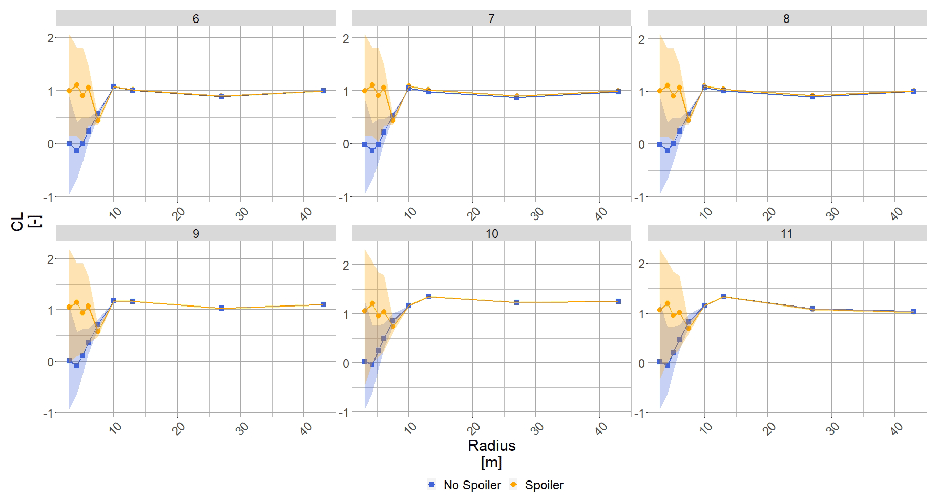
Figure 11The blue square (blue ▪) shows the CL evolution along the blade radius without spoiler, and the orange dot (orange •) shows the CL evolution along the blade radius with spoiler. Each subplot shows the results for a wind speed (m s−1) whose value is given in the title.
2.5.3 Flexible turbine simulations
The second analysis is a fully flexible turbine with turbulent wind using OpenFAST. The tool TurbSim (see Jonkman and Buhl, 2005) developed by NREL is used to generate 10 min long three-dimensional turbulent wind fields for each wind speed. The box representing the wind field is 150 m wide and high subdivided in 50 points and 600 s long. The IEC Kaimal model is used as the spectral model thanks to the directly available IEC class requirements (here IEC class II chosen). The underlying assumption is that the atmospheric conditions are considered neutral following the Monin–Obukhov similarity theory as detailed in Wharton and Lundquist (2012), Holtslag et al. (2014), and Diaz et al. (2010).
After running all the turbine configurations, a deep aerodynamic analysis is possible as many sensor outputs are available. For brevity reasons only a small sample of all the available results will be presented. The multiple polar “states” (mean, maxi, mini) allow assessment of the variation around the mean value, giving a measure of unsteadiness. First, the rigid turbine loads, power and AEP are analysed. Secondly, the flexible turbine fatigue impact is analysed.
3.1 Rigid turbine
In Figs. 11 to 13, the x axis represents the blade radius, the y-axis represents the considered sensor output and each subplot represents a wind speed whose value is given in the title, from 6 to 11 m s−1.
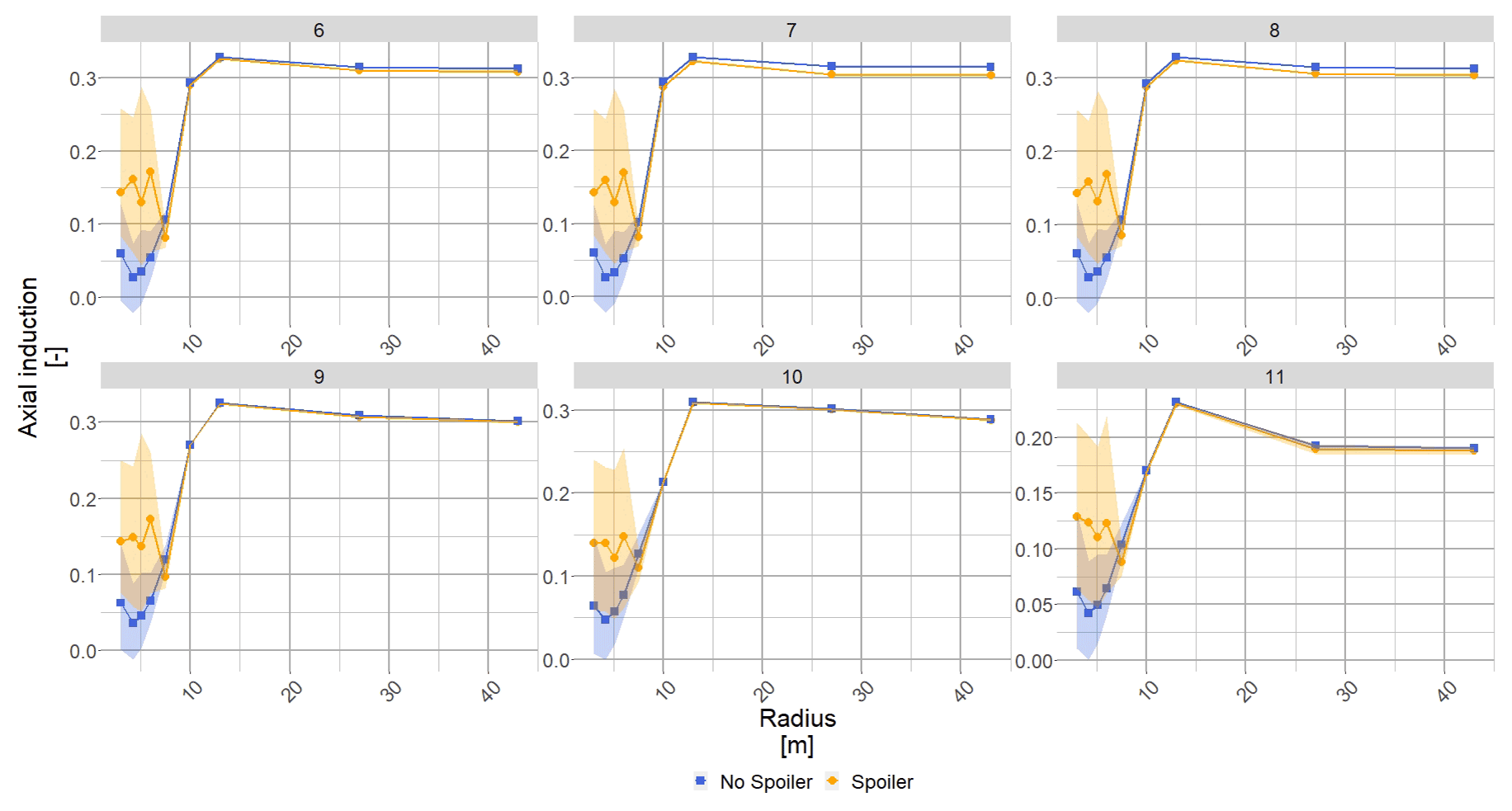
Figure 12The blue square (blue ▪) shows the a evolution along the blade radius without spoiler, and the orange dot (orange •) shows the a evolution along the blade radius with spoiler. Each subplot shows the results for a wind speed (m s−1) whose value is given in the title.
3.1.1 Aerodynamic parameters
The lift coefficient of the no-spoiler case shows very low values inboard, as expected from very thick aerofoils. After the radial position R7.2 ( %), both curves merge, describing the end of the spoiler effect. For the spoiler case, the mean CL increases to relatively high values, especially for such inboard sections, (). However, the associated variation increases drastically. Indeed, the variation for the no-spoiler case was while in the spoiler case the variation is close to (see Fig. 11). A similar outcome is seen for the drag coefficient (not shown here). The large variation in CL is a consequence of the polar unsteadiness.
The axial induction, a, is a key aerodynamic metric for turbine analysis. Through this parameter it is possible to have information about the sectional energy extraction and the sectional turbine loading. The energy extraction is at its maximum when , according to the Betz limit, and the loads increase significantly beyond a=0.4 following the highly loaded rotor relationship (Glauert correction). Therefore, most turbine manufacturers aim for an induction factor value close to the optimal , when in power production mode. After the pitch optimization, the turbine runs close to optimal axial induction for the outer part of the blade.
The no-spoiler case show very low induction values at the root of the blade due to the cylinder shape: low lift coefficient and high drag values. The blade's inboard is not efficient to extract energy but the expected load level is consequently low. Where the spoiler is installed the induction increases, and similarly to the lift coefficient the upper band of the variation due to the polar unsteadiness is close to the optimal induction. The average induction level at the spoiler location is close to a=0.2, which is a significant improvement compared to the no-spoiler case where the induction level is close to 0 (see Fig. 12). The relative variation area is similar compared to the lift coefficient: and still a lot larger than the no-spoiler case.
Interestingly, for 6, 7 and 8 m s−1, the axial induction after the radial position R10 is lower for the spoiler than for the no-spoiler case. This is due to the pitch optimization. The objective function was to maximize power and not try to reach optimal induction. The best trade-off between the spoiler power generation and the blade outboard power generation is when the blade outboard is not at its optimal point to allow for the blade inboard to play a more important role. It also means that the blade tip is slightly less loaded, as can be seen in Sect. 3.1.2. However, the axial induction is still very close to its optimal value (a=0.3).
3.1.2 Aerodynamic static loads
The local out-of-plane force (FX) is calculated, and its evolution against the radius for several wind speeds is shown in Fig. 13. Through the momentum theory and the axial induction, FX is directly proportional to the power production. The bare blade design intent showed very low normal forces at blade root level with an almost constant increase along the span past R10. After the spoiler installation the local force increases significantly, despite being significantly lower than the outer part of the blade. Due to the different pitch settings between both blades, the spoiler case shows a slightly lower force towards the blade tip.
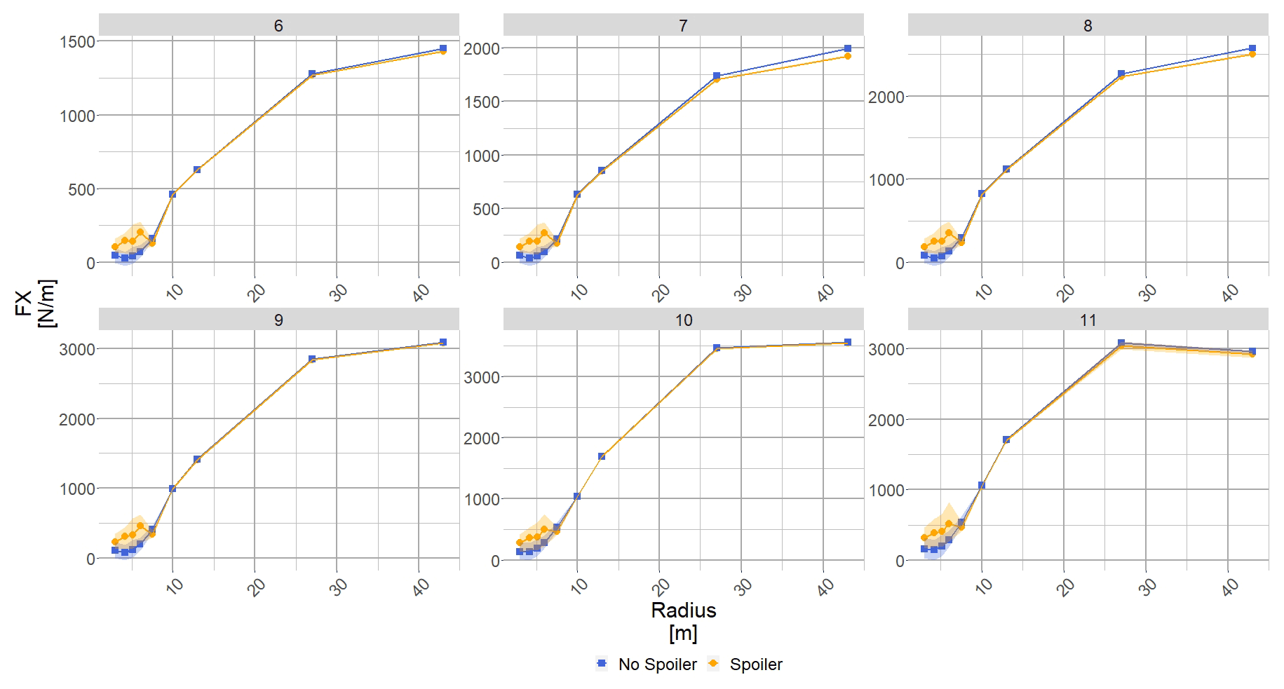
Figure 13The blue square (blue ▪) shows the force normal to the rotor plane evolution along the blade radius without spoiler, and the orange dot (orange •) shows the normal force to the rotor plane evolution along the blade radius with spoiler. Each subplot shows the results for a wind speed (m s−1) whose value is given in the title.
3.1.3 Integrated load: root bending moment
The previous figures showed the results at the aerofoil level, and the next phase of the analysis will focus on the integrated values.
The flapwise root bending moment (RBM) is a critical parameter for blade design and is directly linked to FX through Eq. (4):
where FX(r) is the local out-of-plane force and r the local radius considered.
The unsteadiness caused by the spoiler does not seem to be reflected at rotor level, and the coloured area around the mean value is almost nonexistent. Also, because the change is very small, both curves seem overlapped in Fig. 14. The vertical bars show the difference between the mean RBM values for the spoiler and no-spoiler case. Except around 5 m s−1, the use of a spoiler tends to decrease the RBM slightly (right-hand side vertical axis).
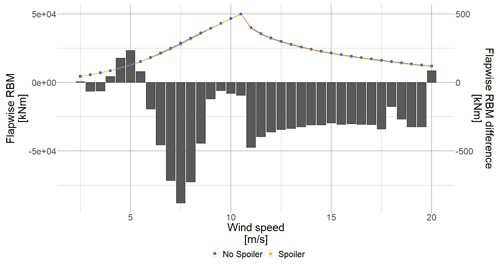
Figure 14The blue square (blue ▪) shows the flapwise root bending moment evolution without spoiler, and the orange dot (orange •) shows the flapwise root bending moment evolution with spoiler. The black bars show the difference between the spoiler and no-spoiler case for each wind speed.
The lower RBM value in the spoiler case is explained thanks to the pitch settings, and the same explanation as for the out-of-plane force FX holds for the RBM. The spoiler case pitch settings are less “aggressive” due to the higher power produced thanks to the blade inboard. The blade outboard, where most of the power is generated, experiences a lesser angle of attack than the no-spoiler case. Therefore, the local load generated by the outer part of the blade is smaller in the no-spoiler case than in the spoiler case. After the integration, performed using Eq. (4), the RBMno spoiler is higher than RBMspoiler.
3.1.4 Power curve and energy production
The mean power curves for the no-spoiler and spoiler configuration can be plotted (see Fig. 15). Both curves are very close to each other; the vertical bars shows that the spoiler does produce more energy on average, albeit a small amount (power difference on the right-hand axis). The error bars show the variation in power due to the different polar states used; i.e. the top of the error bar is the power difference between the spoiler and the no-spoiler case using the maximum aerodynamic coefficient polar.
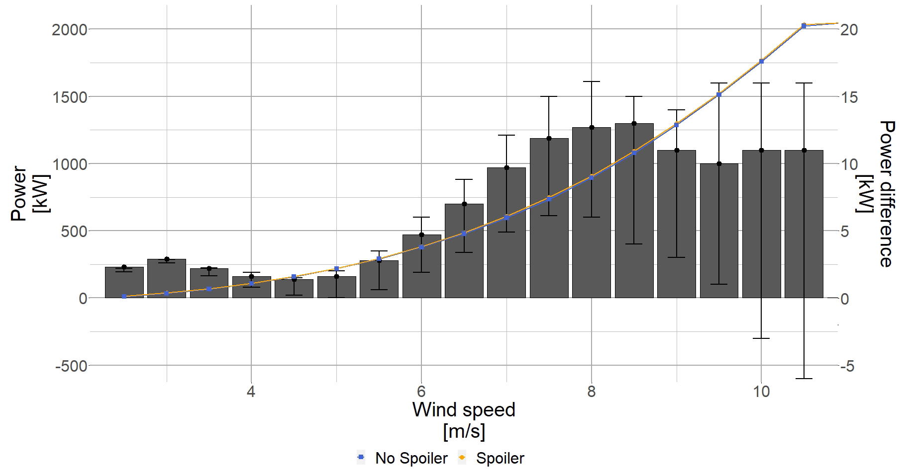
Figure 15Power curve close-up for the low wind speeds. The blue square (blue ▪) shows the power curve without spoiler, and the orange dot (orange •) shows the power curve with spoiler. The black bars show the difference between the mean spoiler and mean no-spoiler case.
It is to be noted that, interestingly, the power gain of approximately 1 %, for wind speeds up to up to 8 m s−1, is similar to the CL gain thanks to the spoiler presented in Fig. 11. Closer to rated power, the power gain reduces.
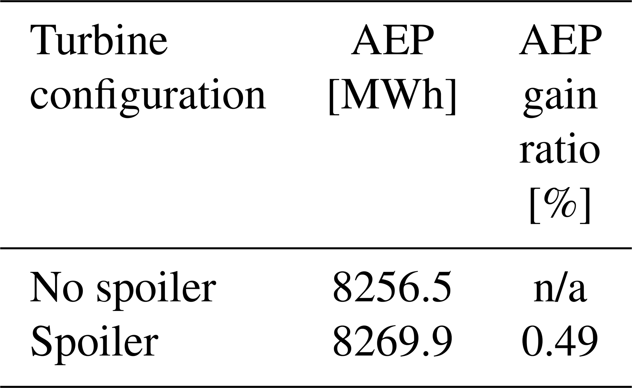
After integrating the mean power curves over a year simulating a wind site condition IEC class II (Weibull shape factor = 0.2 and average wind speed = 8.5 m s−1), the AEP impact can be seen in the Table 4. On average, the spoiler produces 0.49 % AEP more than the no-spoiler case, assuming maximum power extraction settings.
Turbine unsteadiness definition
When using BEM, one cannot use a time-varying description of each angle of attack during the iterative procedure. Using several steady-state polars representing the different possible aerodynamic coefficients allowed for a first estimation of the variation due to the unsteadiness. Analysing the loads or the different aerodynamic metrics (such as presented in Sect. 3.1.1 and 3.1.2) using three different polar states independently is acceptable because the data represent instantaneous “snapshot” values. However, to integrate the results in time, to calculate the mean thrust or the AEP, this assumption cannot hold. Indeed, assuming that the aerodynamic coefficient time variation is periodic, as illustrated in Fig. 3, then after integration all oscillations cancel out. Therefore, the unsteadiness caused by the spoiler on time-integrated quantities cannot be assessed. For this reason, the following method has been applied to give a measure of the variation caused by the spoiler, using the AEP as an example.
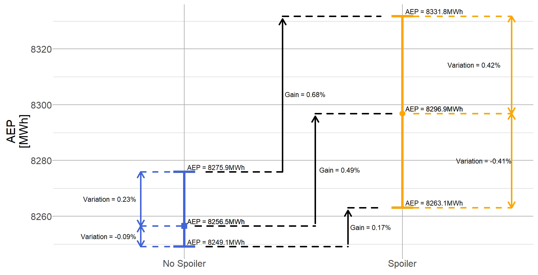
Figure 16Detailed AEP gain and variation for all configurations assuming a wind class IEC II.
The total variation in power for each wind speed is found by . Then, knowing the Weibull site characterization it is possible to calculate the probability of each wind speed occurring over a year: pr(WS). Combining both, the weighted Weibull average total variation around the mean value is found (see Eq. 5).
where δP is the Weibull weighted average power variation, ΔPWS is the power range over a wind speed, WS is the considered wind speed and pr(WS) is the wind speed occurrence probability.
Table 5 shows that the spoiler addition increases the inherent variation around the mean value for the AEP.
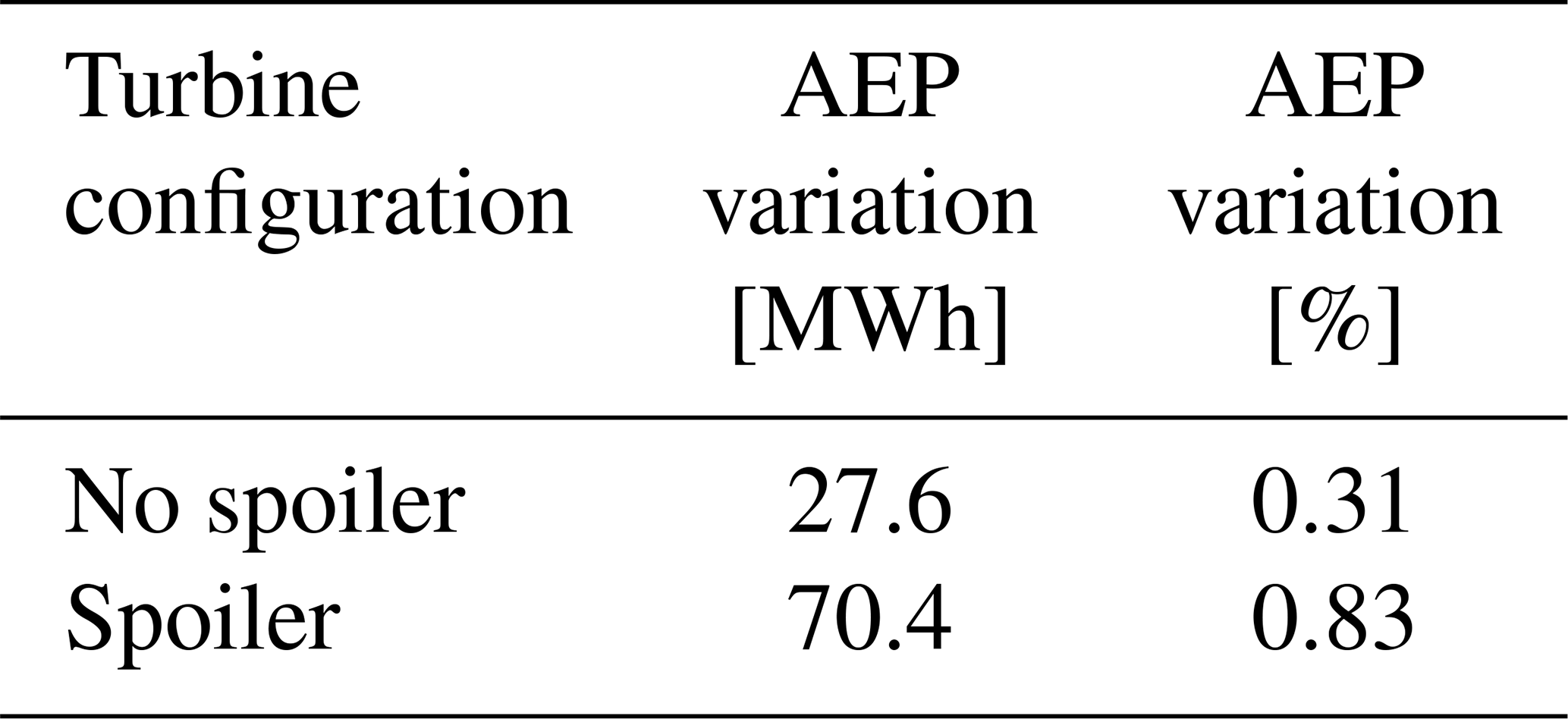
Figure 16 gives more details about the AEP variation than Table 5, which gives the overview. The central symbol represents the AEP calculated using the mean aerodynamic coefficient polar. The error bars represent the AEP calculated when using the minimum and maximum aerodynamic coefficient polar as explained in Table 1. Comparing each configuration (black lines), the AEP gain using mean aerodynamic coefficients polar is 0.49 %, the AEP gain using minimum aerodynamic coefficients polar is 0.17 % and the AEP gain using maximum aerodynamic coefficients polar is 0.68 %. Within each configuration (blue and orange arrows) the overall variation due to the unsteadiness also changes: the spoiler increases the variation in the AEP calculation. The AEP variation is ±0.4 % in the spoiler case, while in the no-spoiler case, the variation is approximately halved (+0.23 % and −0.09 %).
One should note that performing AEP calculation should “smooth out” any variation due to the polar unsteadiness since the power is integrated over a year. Nevertheless, we have chosen to treat each result for each polar state independently in order to define boundaries for the spoiler's potential. The gains presented assume a single turbine operating at maximum power production, as detailed in Sect. 2.5.1, which is unrealistic. Consequently, the actual expected gains will be smaller.
3.2 Flexible turbine
As seen in the previous sections, the rigid modelling shows little AEP benefit of installing the spoiler. However, due to the large increase in the mean local loads and its associated variation introduced by the spoiler, it seems interesting to investigate the damage and fatigue on the turbine. The aeroelastic calculations will be performed by OpenFAST with a fully flexible turbine. The fatigue analysis will focus on the blade only but can be extended to the whole turbine.
3.2.1 Combination method
A method to account for unsteadiness on a rigid turbine has been presented in Sect. 3.1.4, but it can only simulate integrated load. In order to further analyse the spoiler unsteadiness, impact fatigue analysis is necessary. However, the same BEM limitations arise. Here again, we chose to calculate each configuration (no spoiler and spoiler) using the three polars for each wind speed (from 3 to 20 m s−1). Then, thanks to a previously calculated vortex shedding frequency (VSF) for each aerofoil section, a new time series is generated, as detailed below.
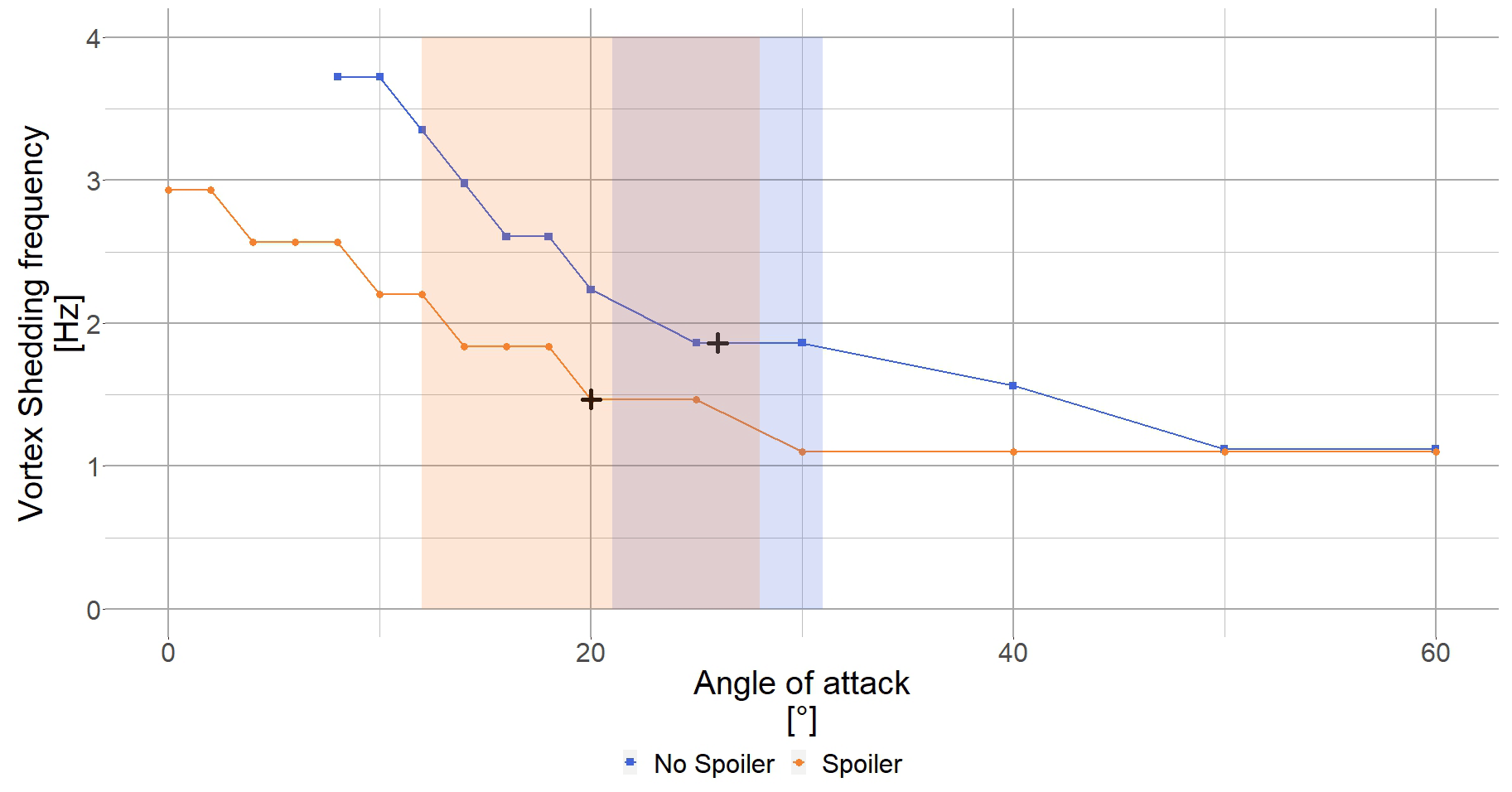
Figure 17Plot of the angle of attack versus the vortex shedding frequency for the no spoiler and spoiler cases, with radial position R6 ( %) calculated in 2D CFD. The blue square (blue ▪) shows the no-spoiler VSF, and the orange dots (orange •) show evolution of the spoiler VSF depending on the angle of attack. The black crosses mark the mean VSF (interpolated VSF at the mean angle of attack of the time series) for each case. The shaded area shows the standard deviation of the angle-of-attack time series.
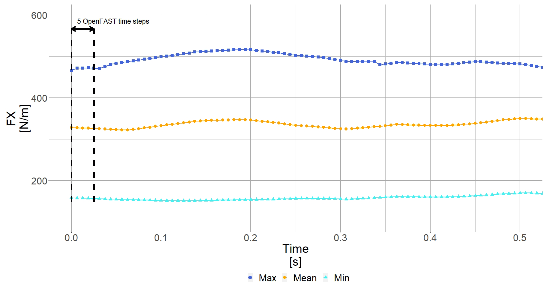
Figure 18OpenFAST time evolution of 0.5 s of the local out-of-plane force (FX) using the maximal, mean and minimal aerodynamic polars.
Vortex shedding frequency (VSF)
In Potentier et al. (2022), the authors showed that a VSF can easily be found for a single aerofoil at a single angle of attack using 2D CFD velocity (or load) time series. Applying the same methodology for all aerofoils and for all angles of attack, 2D CFD load time series were post processed, thereby creating a database of VSF (see Fig. 17). Using the BEM hypothesis of 2D flow, we assume that neither the blade rotation nor the blade deflection change the VSF. Moreover, the turbulent wind speed frequency spectrum is independent from the VSF, and we can therefore perform the interpolation in the time domain between time series rather than in the frequency domain.
Because of the sampling theorem, the OpenFAST sampling output rate must be at least 2 times higher than the highest VSF. The highest calculated VSF of all sections is approximately 60 Hz. To add safety margin, the OpenFAST output is set to be at 160 Hz, which is equivalent to a time step of ΔtOF=0.0063 s.
New OpenFAST time series creation
Once all aeroelastic results are available (Fig. 18), a mean VSF (VSFmean) is determined by interpolating at the mean angle of attack of the mean time series result of the VSF (blue square in Fig. 17). Inverting it leads to a representative time step for the considered wind speed . Then, the original results calculated using maximum, mean or minimum polars are interpolated at new time steps using Δt (Fig. 19).
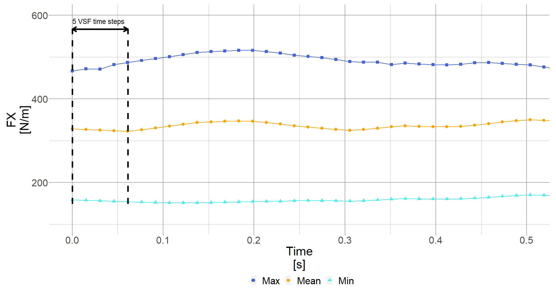

Figure 20Creation of the intermediate time series by alternating between the different interpolated time series.
An intermediate time series is generated, for each sensor. Again, supposing a periodic variation in the lift and drag coefficients, we assume that the first aerodynamic coefficient “seen” by the aerofoil is from the maximum polar, and it then changes to the mean polar and finally the minimum polar and varies following this cycle for 600 s. Such behaviour leads to the creation of the pink curve in Fig. 20.
One final numerical manipulation is necessary because all intermediate time series created possess different VSF and therefore different Δt values by re-sampling them at the same OpenFAST sampling rate (ΔtOF=0.0063 s). Because the turbulent wind speed frequency spectrum is independent of the VSF, we can perform the interpolation in the time domain rather than in the frequency domain. We thus ensure possible further analysis (Fig. 21).
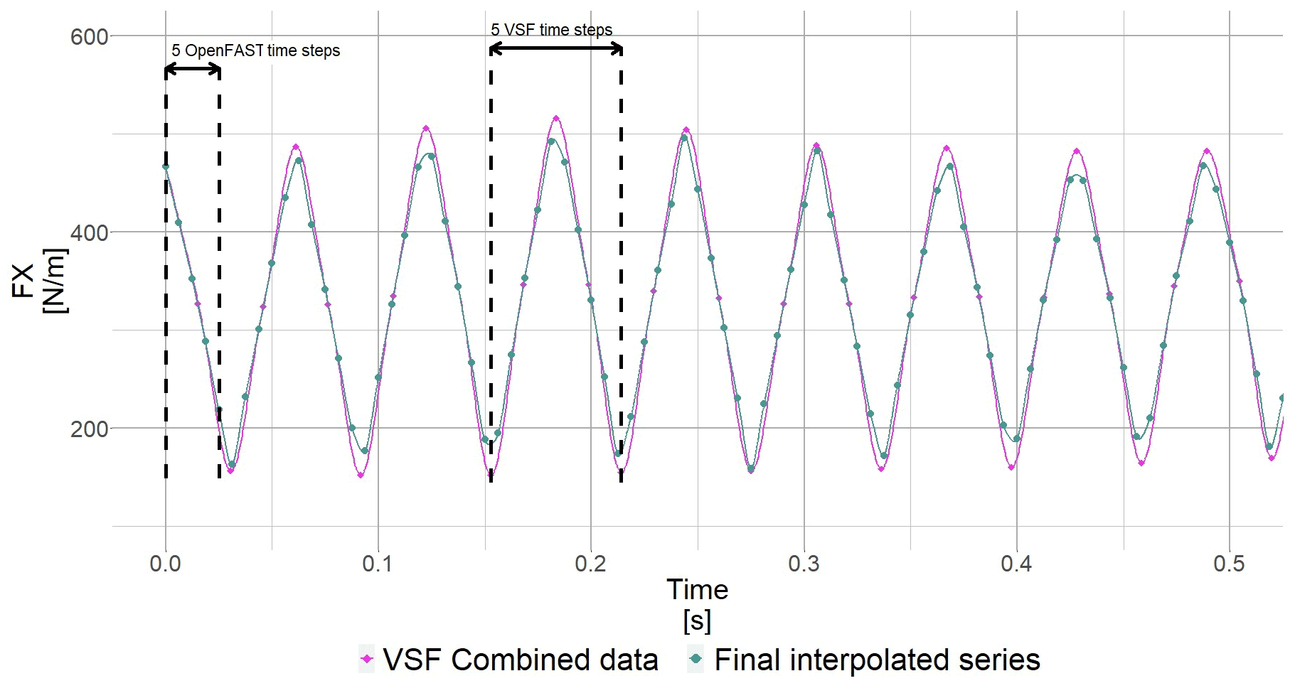
Figure 21Generation of the final time series using the sampling rate from OpenFAST (ΔtOF=0.0063 s).
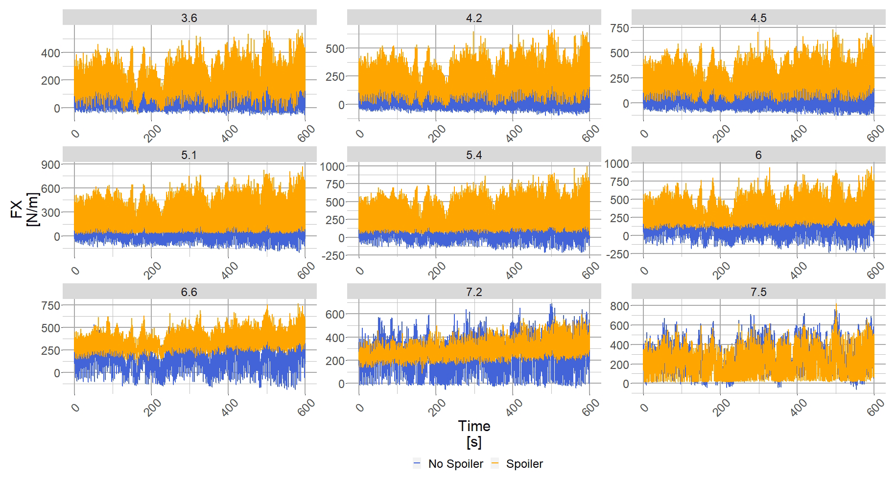
Figure 22OpenFAST output normal force to the rotor plane for an average horizontal wind speed of 8 m s−1 (hub height). The blue square (blue ▪) shows the blade results without spoiler using the combination method, and the orange dot (orange •) shows the blade results with spoiler using the combination method. Each subplot shows the results for a radial location (m) whose value is given in the title.
This method is repeated for each radial position, each wind speed and all local loads. The results presented in the next sections use the data generated by this method.
3.2.2 Normal force results
Figure 22 shows the force normal to the rotor plane (FX) for a 600 s long OpenFAST simulation with an average horizontal wind speed of 8 m s−1 (hub height). Each subplot shows a radial location, from R=3.6 to R=7.5 (from % to %), and the horizontal axis shows the time spent in the simulation. FX is clearly higher in the spoiler case regardless of the spanwise location.
Figure 23 compares the power spectral density (PSD) for the spoiler case using either the mean aerodynamic polar results or the combination method results. At low frequencies the PSDs are overlapped, since the same turbulent wind speed was used in all aeroelastic simulations. However after the VSFmean is reached, the combination method shows clear peaks and harmonics. The curve trend also shows the same downward behaviour at higher frequencies. The higher energy in the spectrum for the combination method hints at higher fatigue loads for the combination method than using the OpenFAST results directly.

Figure 23OpenFAST output normal power spectral density of the normal force to the rotor plane for an average horizontal wind speed of 8 m s−1 (hub height). The blue square (blue ▪) shows the blade results with the combination method for the spoiler, and the orange dot (orange •) shows the blade results for the mean spoiler. Each subplot shows the results for a radial location (m) whose value is given in the title.
3.2.3 Fatigue results
After running in OpenFAST all wind speeds for both turbine configurations and generating the new time series as described in Sect. 3.2.1, it is possible to determine the lifetime impact of the spoiler and its associated unsteadiness on the turbine. The tool used is Mlife, also developed by NREL (see Hayman, 2012). Similarly to the AEP calculation, we assume that the generated OpenFAST outputs follow a Weibull distribution of an IEC site B (shape factor = 2 and average wind speed = 8.5 m s−1).
The method developed can only account for sectional loads since it relies on vortex shedding frequency. The integrated load such as RBM cannot be associated with any particular VSF.
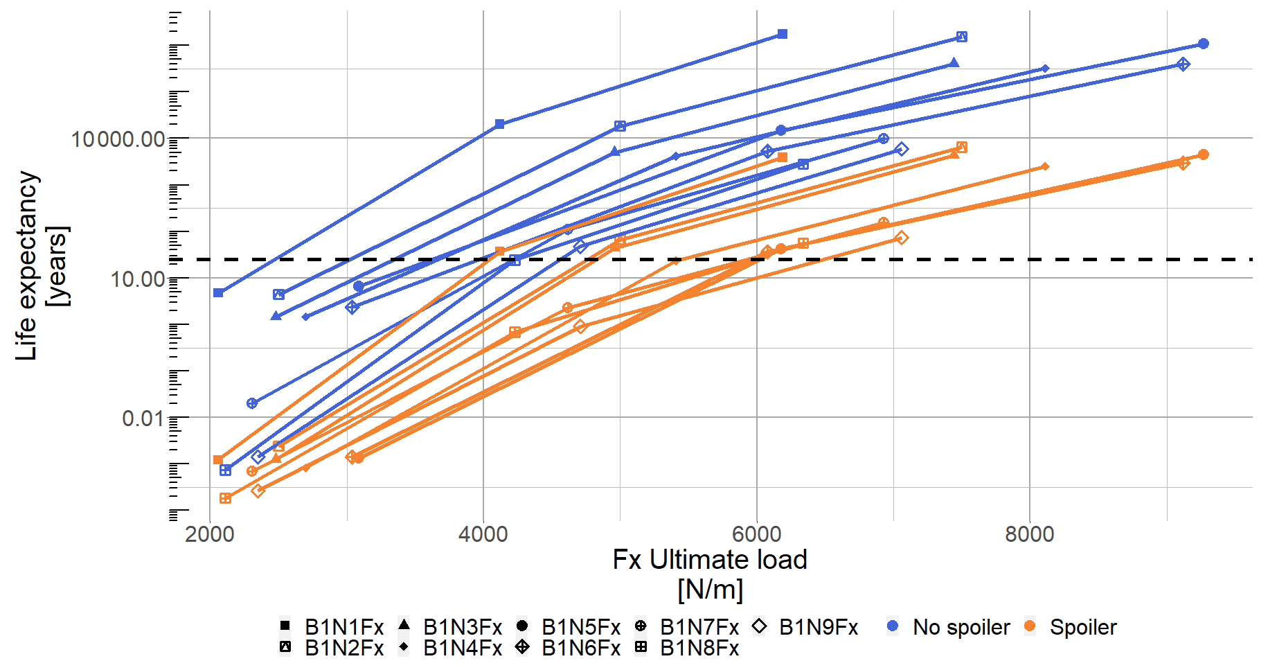
Figure 24Lifetime expectancy evolution with respect to out-of-plane local load. The blue square (blue ▪) shows the blade results without spoiler, and the orange dot (orange •) shows the blade results with spoiler, and each symbol represents a blade nodal output (8.0 % < < 16.7 %).
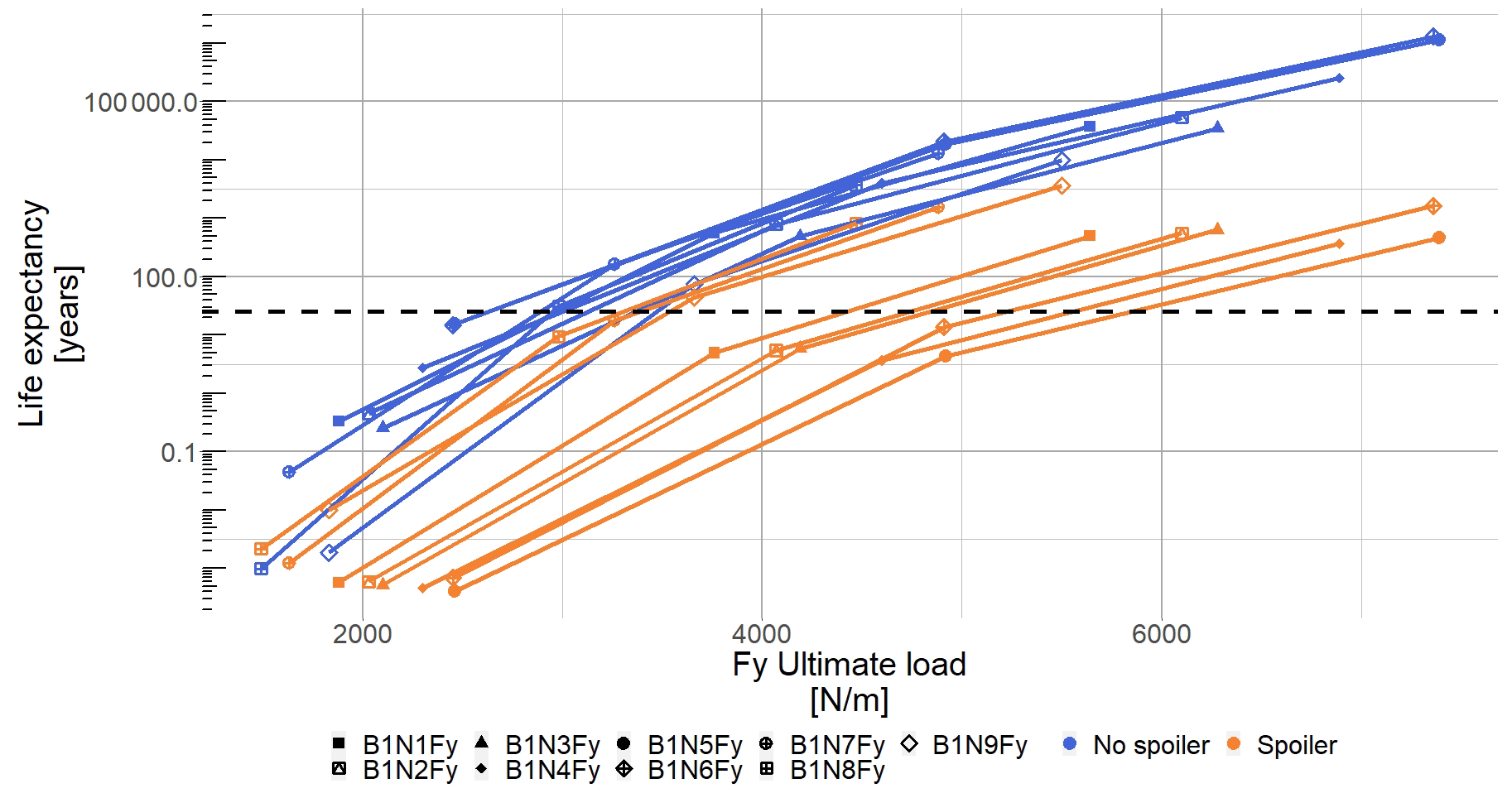
Figure 25Lifetime expectancy evolution with respect to the in-plane local load. The blue square (blue ▪) shows the blade results without spoiler, and the orange dot (orange •) shows the blade results with spoiler, and each symbol represents a blade nodal output (8.0 % < < 16.7 %).
In order to calculate the blade lifetime with the predefined pitch and RPM settings, an ultimate load before rupture for each analysed sensor must be given. Since the material properties are unknown, we used MExtreme (see Hayman, 2015) to extract the highest sectional loads of interest (here FX and FY) seen by the turbine of both cases as first approximation. To assess the evolution of lifetime with respect to the ultimate load, three distinct load values were selected. Using those values for the no-spoiler and spoiler cases, it is now possible to plot the lifetime evolution with respect to the ultimate load for the local out-of-plane force (see Fig. 24) and the local in-plane force (see Fig. 25). The horizontal dashed line shows the usual 25 years design lifetime. The lowest symbol of each coloured line represents the turbine lifetime if it were designed based on the highest load found by MExtreme. The following two points are calculated lifetimes using the initial highest load multiplied by a factor of 2 and 3. As expected, the behaviour is highly non-linear and can reach unrealistic lifetime expectancy. To avoid running fatigue simulation with a very low life expectancy, we choose the loads from the multiplication factor of 2 as baseline for the rest of the analysis (see Appendix B). The Wöhler exponent was kept constant throughout the study to a representative wind turbine blade material: m=10 (see Lloyd, 2010).
Because of the different hypotheses taken, we are only analysing trends and not presenting the direct Mlife results. Therefore a life index (Li) is created by normalizing the outputs of the no-spoiler case to create a baseline; i.e. for each sensor . Then the spoiler case results are normalized by the previously created baseline. Table 6 summarizes the outcome of the fatigue calculation. The second column shows the life index impact of the considered sensor when adding a spoiler.
Here, Li is the life index of the no-spoiler or spoiler case, and j is the section considered.
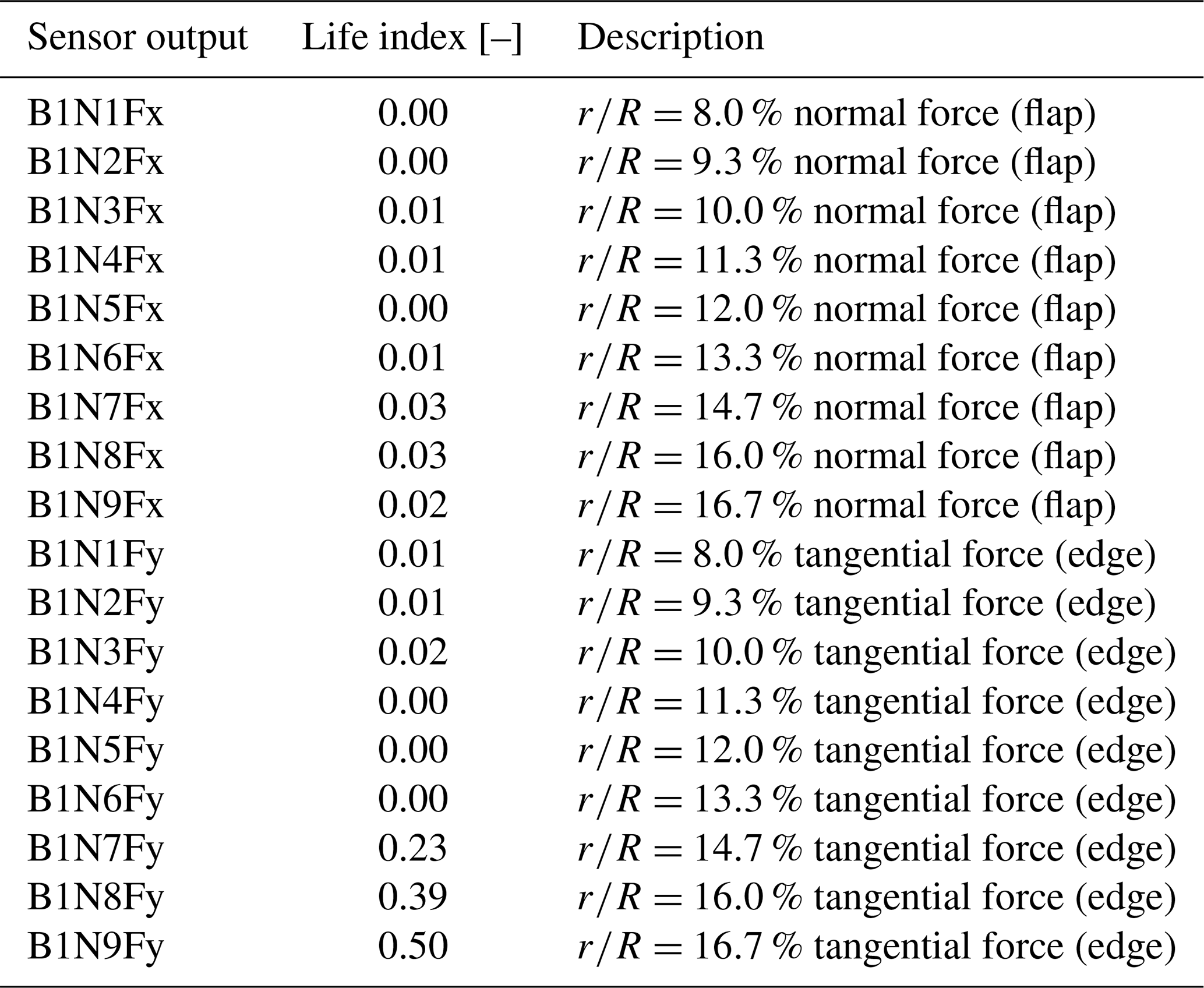
As suspected in Sect. 3.1.2, all local forces see a negative impact after installing the spoilers, and indicates that this specific section will fail before the no-spoiler turbine. Despite the hypotheses and assumptions, the method employed captures the negative impact of the spoiler on the local sections well, which is in line with the blade failures (cracks), seen at the spoiler's end in the field by the ENGIE Green maintenance team. It is to be noted that BEM aeroelastic simulations can model neither the spoiler's glue joint nor the internal elements of the blade (such as spar or web). A dedicated finite element analysis (FEA) would be required to answer the question fully, but such a study is out of the scope of the present paper.
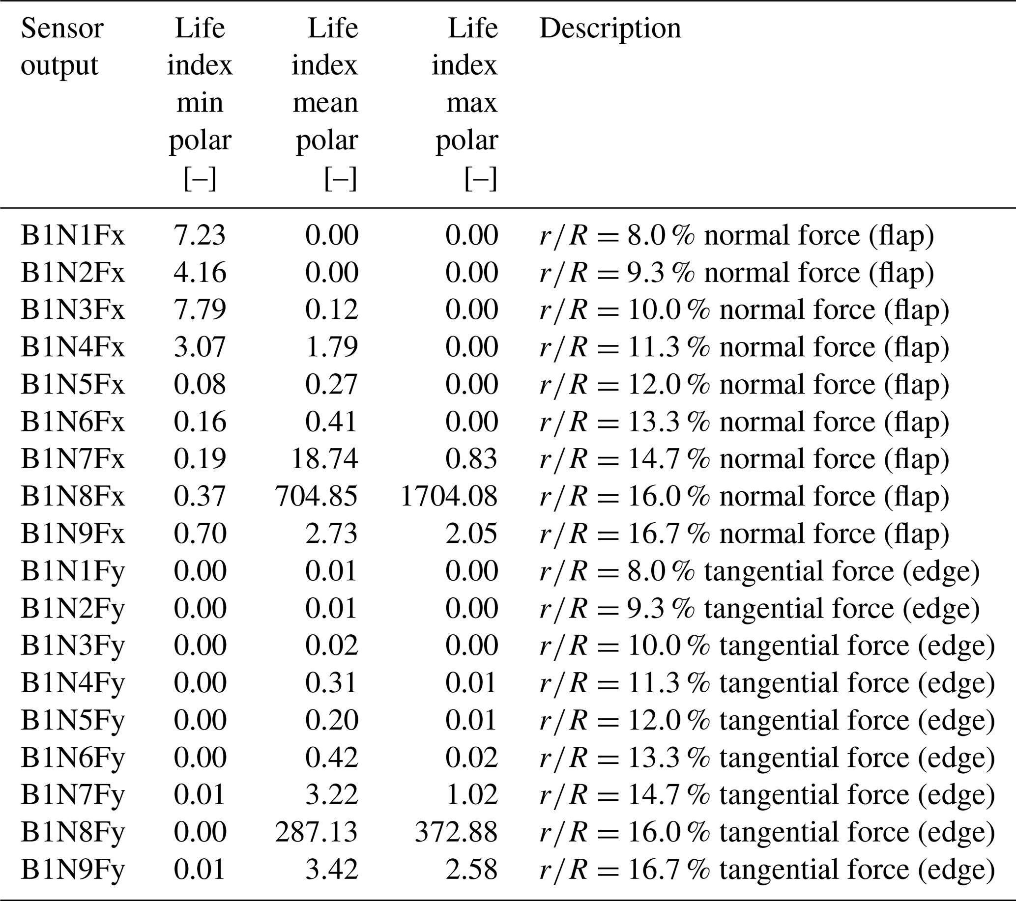
To compare the results of the proposed method, Table 7 shows the same life index calculation when using the steady polar. In some cases the fatigue calculation predicts much higher residual lifetime when adding a spoiler. It appears in contradiction with the analysis performed so far and the damaged blades in the field. It highlights the risk of installing such AAO without knowing the aerodynamic impact and structural consequences.
The authors built an aeroelastic BEM model for a commercial 2 MW turbine retrofitted with root spoilers using a 3D blade scan. The turbine was chosen to address a maintenance problem where blades cracked after installing the spoilers. Regarding the AEP gain and rotor integrated load, the spoiler impact is marginal. The AEP increases by a small amount (≈0.5 %) with a large variation associated. So far, all the efforts made to measure the AEP in the field led to inconclusive results due to the small absolute difference and large dispersion in the power curve measuring method. The integrated loads remain approximately constant, and a small decrease in flapwise root bending moment has even been noted. However, the local loads increase significantly with a large variation around the mean value.
A fatigue analysis has been performed using a novel way of capturing the aerodynamic unsteadiness due to the aerofoil's behaviour. It uses 2D CFD flow characteristics (vortex shedding frequency) as well as the results calculated from three different steady polars (maximum, mean and minimum aerodynamic coefficients). The spoiler increases the already locally present unsteadiness and should not be neglected in the turbine's structural design. The spoiler can be detrimental to the turbine lifetime: retrofitting such devices should be done with care, and the turbine's mechanical properties should be re-evaluated prior to installing the spoiler.
A similar conclusion could be drawn for other aerodynamic add-ons generating a similar amount of unsteadiness; however dedicated studies would be necessary. Also, more studies would be required to quantify the impact height and chordwise position of the spoiler.
Finally, the presented method currently relies on 2D assumptions and BEM calculations, and further studies involving 3D CFD are being carried out to assess the vortex shedding behaviour on a rotor.

Codes and data sets are available on demand.
TP performed the scans post-processing, CFD pre-processing and post-processing, BEM model building, calculations and analysis, and writing of the paper. EG performed CFD verification and helped set up the CFD model. CLB and AF provided feedback from the industrial point of view, and CB helped with proofreading a previous version of the manuscript and physical analysis of the results.
The contact author has declared that none of the authors has any competing interests.
Publisher's note: Copernicus Publications remains neutral with regard to jurisdictional claims in published maps and institutional affiliations.
The authors would like to acknowledge the ANRT (Association Nationale de Recherche Technologique) for their financial support.
This research has been supported by CIFRE (grant no. 2019/1426).
This paper was edited by Alessandro Bianchini and reviewed by two anonymous referees.
Boorsma, K. and Schepers, J. G.: Rotor experiments in controlled conditions continued: New Mexico, J. Phys.: Conf. Ser., 753, 022004, https://doi.org/10.1088/1742-6596/753/2/022004, 2014. a
Burton, T. (Ed.): Wind energy: handbook, J. Wiley, Chichester, New York, ISBN 9780470699751, 2001. a, b
Campagnolo, F.: Wind Tunnel Testing Of Scaled Wind Turbine Models: Aerodynamics And Beyond, PhD thesis, Politecnico Di Milano, Milano, https://www.politesi.polimi.it (last access: 18 August 2022) 2013. a
Canet, H., Bortolotti, P., and Bottasso, C. L.: On the scaling of wind turbine rotors, Wind Energ. Sci., 6, 601–626, https://doi.org/10.5194/wes-6-601-2021, 2021. a
Chaviaropoulos, P. K. and Hansen, M. O. L.: Investigating Three-Dimensional and Rotational Effects on Wind Turbine Blades by Means of a Quasi-3D Navier–Stokes Solver, J. Fluid. Eng., 122, 330–336, https://doi.org/10.1115/1.483261, 2000. a
Dambrine, G.: Impact of Blade Aging on Wind Turbine Production, MS thesis, European Master in Renewable Energy, EUREC Agency, 2010. a
Diaz, A. P., Gryning, S.-E., and Mann, J.: On the Length-Scale of the Wind Profile, Q. J. Roy. Meteorol. Soc., 136, 2119–2131, https://doi.org/10.1002/qj.714, 2010. a
Hand, M. M., Simms, D. A., Fingersh, L. J., Jager, D. W., Cotrell, J. R., Schreck, S., and Larwood, S. M.: Unsteady Aerodynamics Experiment Phase VI: Wind Tunnel Test Configurations and Available Data Campaigns, Tech. Rep. NREL/TP-500-29955, 15000240, NREL, https://doi.org/10.2172/15000240, 2001. a
Hansen, M.: Aerodynamics of Wind Turbines, in: 3rd Edn., Routledge, London, https://doi.org/10.4324/9781315769981, 2015. a, b
Hayman, G. J.: Mlife user's guide, Tech. rep., National Renewable Energy Laboratory, https://www.nrel.gov/wind/nwtc/assets/pdfs/mlife-theory.pdf (last access: 1 February 2022), 2012. a
Hayman, G. J.: MExtreme User's Guide, Tech. rep., National Renewable Energy Laboratory, https://www.nrel.gov/wind/nwtc/assets/downloads/MCrunch_MLife_MExtremes/MExtremesManual.pdf (last access: 1 February 2022), 2015. a
Holtslag, M. C., Bierbooms, W. A. A. M., and van Bussel, G. J. W.: Estimating Atmospheric Stability from Observations and Correcting Wind Shear Models Accordingly, J. Phys.: Conf. Ser., 555, 012052, https://doi.org/10.1088/1742-6596/555/1/012052, 2014. a
Jonkman, B. J. and Buhl, M. L., J.: TurbSim User's Guide, Tech. rep., National Renewable Energy Laboratory, https://doi.org/10.2172/15020326, 2005. a
Jonkman, J., Butterfield, S., Musial, W., and Scott, G.: Definition of a 5-MW Reference Wind Turbine for Offshore System Development, Tech. Rep. NREL/TP-500-38060, 947422, National Renewable Energy Laboratory, https://doi.org/10.2172/947422, 2009. a
Jonkman, J. M., Hayman, G. J., Jonkman, B. J., Damiani, R. R., and Murray, R. E.: AeroDyn v15 User's Guide and Theory Manual, Renew. Energy, 46, https://doi.org/10.15473/1415580, 2015. a
Lloyd, G.: Guideline for the Certification of Wind Turbine, p. 384, https://wordpressstorageaccount.blob.core.windows.net/wp-media/wp-content/uploads/sites/649/2018/05/Session_3_-_Handout_3_-_GL_Guideline_for_the_Certification_of_Wind_Turbines.pdf (last access: 19 August 2022), 2010. a
Loth, E., Fingersh, L., Griffith, D., Kaminski, M., and Qin, C.: Gravo-Aeroelastically Scaling for Extreme-Scale Wind Turbines, in: 35th AIAA Applied Aerodynamics Conference, American Institute of Aeronautics and Astronautics, Denver, Colorado, https://doi.org/10.2514/6.2017-4215, 2017. a
Madsen, H. A., Bak, C., Paulsen, U. S., Gaunaa, M., Fuglsang, P., Romblad, J., Olesen, N. A., Enevoldsen, P., Laursen, J., and Jensen, L.: The DAN-AERO MW Experiments: Final report, DTU Wind Energy, https://orbit.dtu.dk/en/publications/the-dan-aero-mw-experiments-final-report (last access: 10 February 2022), 2010. a
Potentier, T., Braud, C., Guilmineau, E., Finez, A., and Bourdat, C. L.: Analysis of the DANAERO wind turbine field database to assess the importance of different state-of-the-art blade element momentum (BEM) correction models, Energy Sci. Eng., 9, 1477–1500, https://doi.org/10.1002/ese3.908, 2021. a
Potentier, T., Guilmineau, E., Finez, A., Le Bourdat, C., and Braud, C.: High-Reynolds-number wind turbine blade equipped with root spoilers – Part 1: Unsteady aerodynamic analysis using URANS simulations, Wind Energ. Sci., 7, 647–657, https://doi.org/10.5194/wes-7-647-2022, 2022. a, b, c, d, e, f
Simms, D., Schreck, S., Hand, M., and Fingersh, L. J.: NREL Unsteady Aerodynamics Experiment in the NASA-Ames Wind Tunnel: A Comparison of Predictions to Measurements, Tech. Rep. NREL/TP-500-29494, 783409, NREL, https://doi.org/10.2172/783409, 2001. a
Snel, H., Schepers, J. G., and Montgomerie, B.: The MEXICO project (Model Experiments in Controlled Conditions): The database and first results of data processing and interpretation, J. Phys.: Conf. Ser., 75, 012014, https://doi.org/10.1088/1742-6596/75/1/012014, 2007. a
Trodborg, N., Bak, C., Madsen, H., and Skrzypinski, W.: DANAERO MW II Final Report, no. 0027(EN) in DTU Wind Energy E, DTU Wind Energy, https://orbit.dtu.dk/en/publications/danaero-mw-final-report (last access: 10 February 2022), 2013. a
Viterna, L. A. and Janetzke, D. C.: Theoretical and experimental power from large horizontal-axis wind turbines, Tech. Rep. DOE/NASA/20320-41, NASA-TM-82944, 6763041, National Aeronautics and Space Administration, https://doi.org/10.2172/6763041, 1982. a
Wharton, S. and Lundquist, J. K.: Assessing Atmospheric Stability and Its Impacts on Rotor-Disk Wind Characteristics at an Onshore Wind Farm, Wind Energy, 15, 525–546, https://doi.org/10.1002/we.483, 2012. a