On the measurement of stability parameter over complex mountainous terrain

Atmospheric stability has a significant effect on wind shear and turbulence intensity, and these variables, in turn, have a direct impact on wind power production and loads on wind turbines. It is therefore important to know how to characterise atmospheric stability in order to make better energy yield estimation in a wind farm.

Based on the research-grade meteorological mast at Alaiz (CENER's test site in Navarre, Spain) named MP5, this work compares and evaluates different instrument set-ups and methodologies for stability characterisation, namely the Obukhov parameter, measured with a sonic anemometer, and the bulk Richardson number based on two temperature and one wind speed measurement. The methods are examined considering their theoretical background, implementation complexity, instrumentation requirements, and practical use in connection to wind energy applications. The sonic method provides a more precise local measurement of stability while the bulk Richardson is a simpler, robust and cost-effective technique to implement in wind assessment campaigns. Using the sonic method as a benchmark, it is shown that to obtain reliable bulk Richardson measurements in onshore sites it is necessary to install one of the temperature sensors close to the ground where the temperature gradient is stronger.

1 Introduction

The vertical wind profile and the turbulence intensity in the atmospheric boundary layer (ABL) are two of the main physics aspects driving wind energy production and turbine loads. The vertical wind profile is especially important since rotors are getting bigger and hub heights are getting higher, making it invaluable to know the wind speed at hub height. The vertical wind profile shape and turbulence intensity can directly influence wind turbine production but also wind turbine loads, affecting the wind turbine's lifetime. Despite the fact that the IEC standard (IEC61400-1 (ED4) 2019, 2019) specifies a power law vertical model independent of atmospheric stability to perform load calculations, the dependence of this and, in turn, the turbulence intensity with atmospheric stability is widely demonstrated (Emeis, 2013; Lange et al., 2004b; Peña and Hahmann, 2012). In addition several studies have demonstrated the impact of atmospheric stability on wind resource assessment (Lange et al., 2004a), wind turbine power curves and annual energy production (AEP) calculations (Martin et al., 2016; Schmidt et al., 2016); wind turbine loads (Kelly et al., 2014; Sathe et al., 2013) and wind turbine wakes (Abkar and Porté-Agel, 2015; Hansen et al., 2010; Machefaux et al., 2016). This is why the wind industry is developing models and methods to include the effect of atmospheric stability in the layout design and energy yield assessment. These methodologies and models require the characterisation of the probability distribution of atmospheric stability at each site. Therefore different methods and parameters are used to describe atmospheric stability without an industry-wide convention about which one is the most appropriate.

According to Monin and Obukhov similarity theory (MOST) (Foken, 2006; Monin and Obukhov, 1954), stability can be estimated in terms of the inverse of Obukhov length that can be calculated with vertical fluxes of heat and momentum obtained with the eddy covariance method. To obtain the necessary high-frequency measurements of wind speed vector components and temperature, sonic anemometers are used, which is why this calculation method is called the “sonic method”.

Another measure for stability is the Richardson number, which as Bardal et al. (2018) explains, according to Stull (1989) has several formulations: the flux Richardson number, gradient Richardson number and bulk Richardson number. The latter is based on one height wind speed measurement and two temperature measurements, one from the air at one height and the other from the ground or water surface.

In the wind energy context some studies have been done about how to measure the stability and their influence in the turbulence intensity and vertical wind profile. However, most of these studies have been carried out in offshore sites (Peña and Hahmann, 2012; Sanz Rodrigo et al., 2015; Sathe et al., 2011), finding relationships (Grachev and Fairall, 1997) between the Obukhov length and the Richardson bulk number that facilitate the characterisation of stability without the need of sonic anemometer. This is convenient, because although the sonic anemometer has many advantages (Cuerva et al., 2006), it adds complexity in terms of use and data management, and it increases the cost of the long-term site assessment campaigns.

For onshore sites there are few studies that analyse how to characterise atmospheric stability, and those that exist are on simple topography in coastal areas (Bardal et al., 2018).

Although the behaviour of wind flow over complex terrain is widely studied, as Finnigan et al. (2020) summarise, and discussed in recent publications about the influence of atmospheric stability in wind farms located in complex terrain (Han et al., 2018; Menke et al., 2019; Radünz et al., 2020, 2021), there are no references that analyse in detail how to characterise atmospheric stability according to different instrumentation requirements.

Measuring atmospheric stability in complex terrain has some challenges (compared to flat terrain): one of them is the fact that the MOST is developed for horizontally homogeneous and flat terrain, and in complex terrain vertical wind speed can be due to stability or sloping terrain. Therefore, vertical fluxes will be “contaminated” by terrain effects. This can be mitigated by using good measurement practices (data quality, coordinate systems and post-processing options) (Stiperski and Rotach, 2015).

This study presents atmospheric stability characterisation from one mountainous site obtained using two methods: the sonic method and the Richardson bulk number. Measurements of different heights have been used to see the influence of this parameter on the results.

The place used in this study meets the characteristics of a typical complex terrain site for wind energy deployment. The 118 m high MP5 reference meteorological mast, as is explained in other articles by Sanz Rodrigo et al. (2013) and Santos et al. (2020), is equipped with wind (cup and 3D sonic anemometer) and temperature measurements distributed along six vertical levels: 2, 40, 80, 90, 100 and 118 m above the ground level (a.g.l.), enabling the comparison between Richardson bulk number and the sonic method to evaluate atmospheric stability.

Special focus is given to explaining the post-processing methodologies to derive stability from raw data considering a fast-response sonic anemometer in a complex terrain.

2 Atmospheric stability definitions

2.1 The Obukhov length

Monin and Obukhov (M–O) (Monin and Obukhov, 1954) introduced the Obukhov length L to characterise atmospheric stability, which is proportional to the height above the surface at which the production of turbulent energy from buoyancy dominates over mechanical shear production of turbulence (Stull, 1989), and it is defined as

$$\begin{array}{}\text{(1)}& {\displaystyle }L=-{\displaystyle \frac{u_{\ast }^{\mathrm{3}}}{\mathit{\kappa }\frac{g}{{\mathrm{\Theta }}_{\mathrm{0}}}\stackrel{\mathrm{‾}}{w^{\prime }{\mathit{\theta }}^{\prime }}}},\end{array}$$

where $g=\mathrm{9.81}{\mathrm{ms}}^{-\mathrm{2}}$ is the acceleration due gravity, κ=0.41 is the von Karman constant, u^* is the friction velocity, Θ₀ is the surface potential temperature and $\stackrel{\mathrm{‾}}{w^{\prime }{\mathit{\theta }}^{\prime }}$ is the heat flux. The dimensionless height $\mathit{\zeta }=z/L$ is used as a stability parameter, where ζ<0 indicates unstable, ζ>0 stable and ζ=0 neutral conditions.

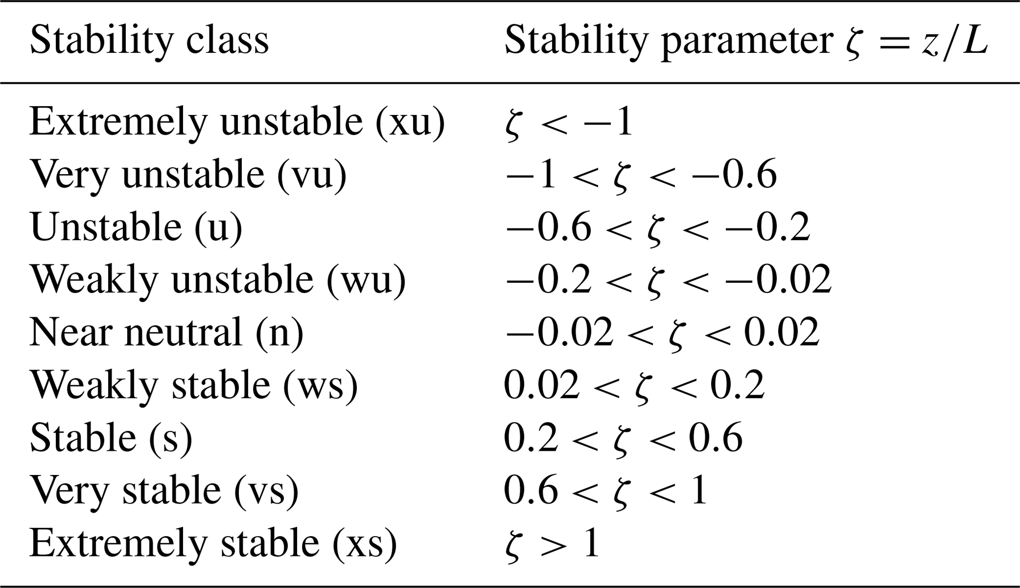
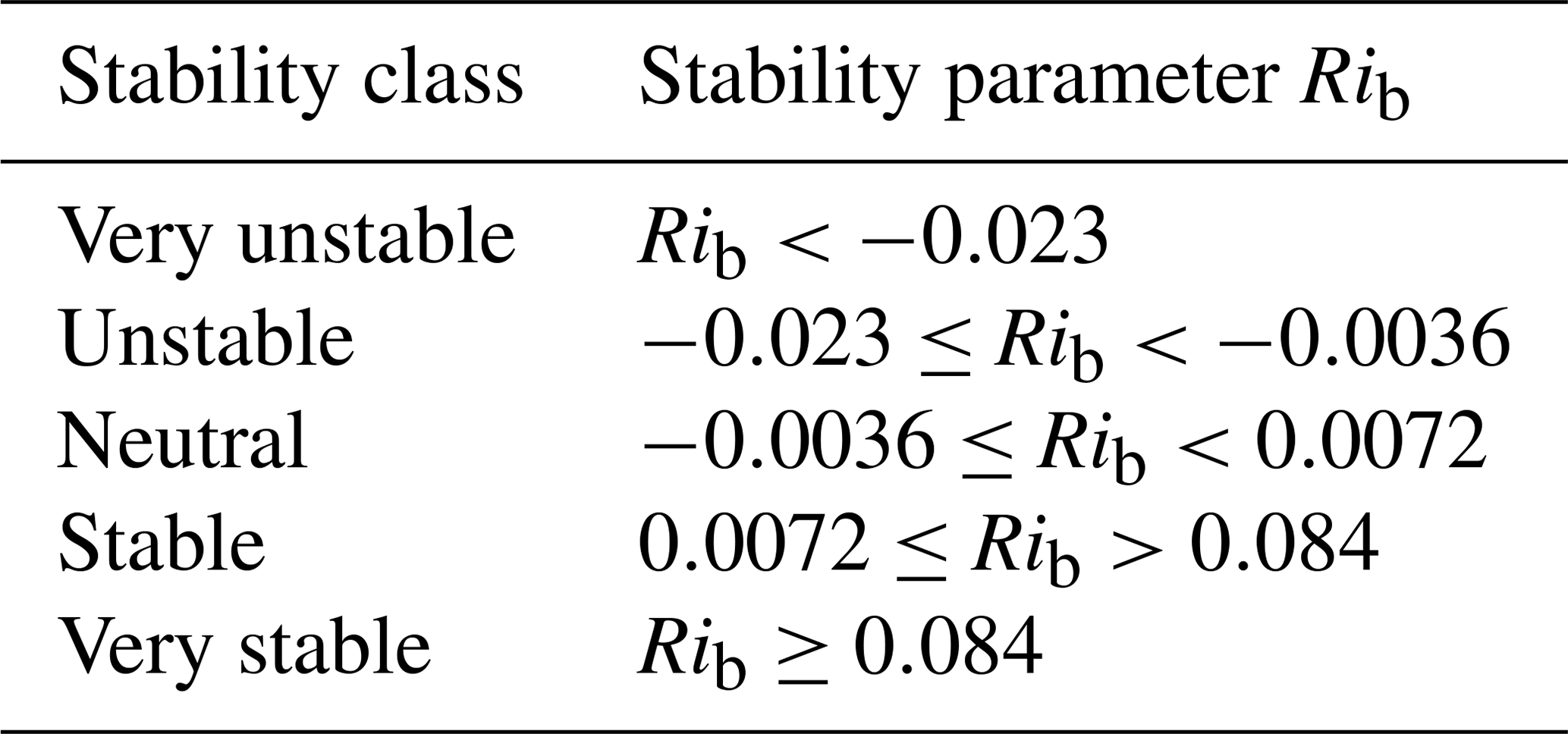
Table 1 shows the (Sorbjan and Grachev, 2010) stability classification, proposing four regimes in stable conditions. This classification is also followed by Sanz Rodrigo et al. (2015) assuming a symmetric classification in the unstable range. Sanz Rodrigo et al. (2015) shift the “extremely unstable and stable” regime limit to $\left|\mathit{\zeta }\right|=\mathrm{1}$ in order to avoid contamination of the large scatter found on the high ends of the scale to the “very unstable and/stable” class. An additional limit is added at $\left|\mathit{\zeta }\right|=\mathrm{0.2}$ to give higher resolution in the most frequent stability range. For consistency, we shall adopt the same classification used in Sanz Rodrigo et al. (2015) to facilitate the comparison with offshore conditions.

Table 1 Classification of atmospheric stability adapted from Sorbjan and Grachev (2010).

Using sonic anemometers and the eddy covariance technique, the Obukhov length can be obtained. In this way, stability is evaluated locally based on turbulent fluxes averaged over periods from 10 min to 1 h to integrate the kinetic energy in the microscale turbulence range.

A sonic anemometer can be used in complex terrain to derive the local Obukhov length. Following the planar fit method of Wilczak et al. (2001), momentum fluxes should be calculated in the mean streamline plane and heat fluxes in the true vertical coordinate system. If the streamline plane can be known a priori, from a wind direction sector with uniform slope, the planar fit method can be used to infer the mounting tilt angle and correct for it to reduce the uncertainty on the vertical fluxes.

2.2 Bulk Richardson number

The bulk Richardson number Ri_b is a form of the Richardson number that is widely used for characterising stability for its simplicity, defined in terms of a potential temperature difference and a single velocity level:

$$\begin{array}{}\text{(2)}& {\displaystyle }{\mathit{\text{Ri}}}_{\mathrm{b}}=-{\displaystyle \frac{gz\mathrm{\Delta }\mathrm{\Theta }}{{\mathrm{\Theta }}_{\mathrm{0}}\stackrel{\mathrm{‾}}{{\overline{U}}^{\mathrm{2}}}}}.\end{array}$$

Here, as proposed (Sanz Rodrigo et al., 2015), the height z is taken here as the mean height between the two levels of temperature, and ΔΘ is derived from the water–air or surface–air temperature difference.

As Bardal et al. (2018) propose, the general empirical relations from Businger et al. (1971) slightly modified by Dyer (1974) have been used to relate ζ with the Ri_b.

$$\begin{array}{}\text{(3)}& {\displaystyle }\mathit{\xi }=\left\{\begin{array}{l}{\mathit{\text{Ri}}}_{\mathrm{b}},{\mathit{\text{Ri}}}_{\mathrm{b}}<\mathrm{0}\\ \frac{{\mathit{\text{Ri}}}_{\mathrm{b}}}{\mathrm{1}-\mathrm{5}{\mathit{\text{Ri}}}_{\mathrm{b}}},\mathrm{0}<{\mathit{\text{Ri}}}_{\mathrm{b}}<\mathrm{0.2}\end{array}\right.\end{array}$$

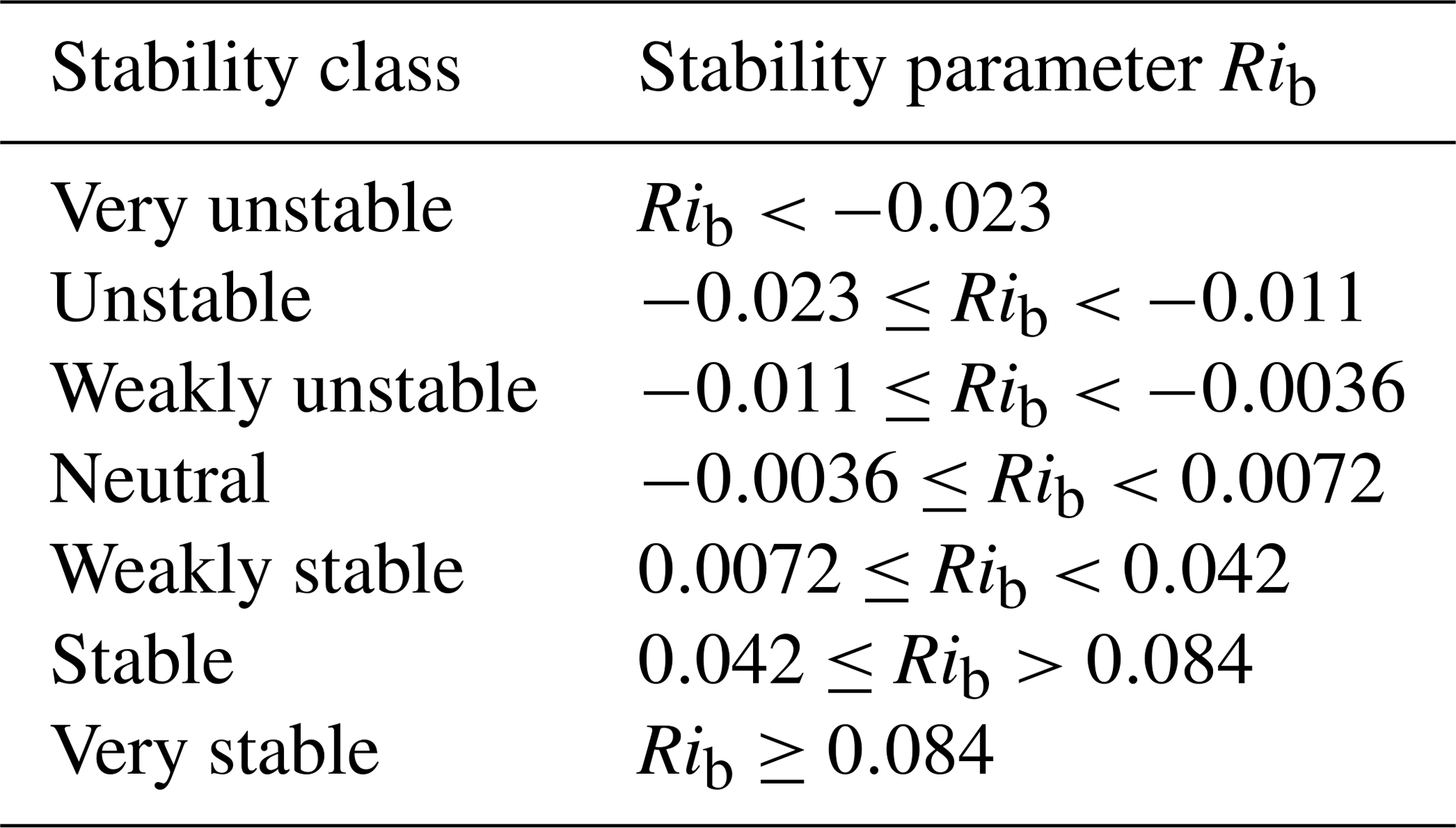
Alternatively Ri_b can be used to directly do a stability classification. Mohan (1998) has proposed a seven-class stability classification methodology (Table 2), which has been accepted by the scientific community as shown by Ruisi and Bossanyi (2019).

Table 2 Classification of atmospheric stability (Mohan, 1998).

3 The Alaiz site

The MP5 mast is located (42^∘41.7^′ N, 1^∘33.5^′ W) at the top of Alaiz mountain in the region of Navarre (Spain), around 15 km SSE from Pamplona in the CENER's experimental wind farm. The prevailing wind directions are from the north and from the south. To the north there is a large valley at around 700 m lower altitude. To the south, complex terrain is found with the presence of some wind farms; the closest one situated 2 km behind the row of six wind turbine stands of the test site (see Fig. 1). As is explained by Sanz Rodrigo et al. (2013), the wakes from this wind farm can be considered well mixed with the boundary layer flow in most conditions, so additional turbulence in MP5 due to wakes from neighbouring wind farms is not expected.

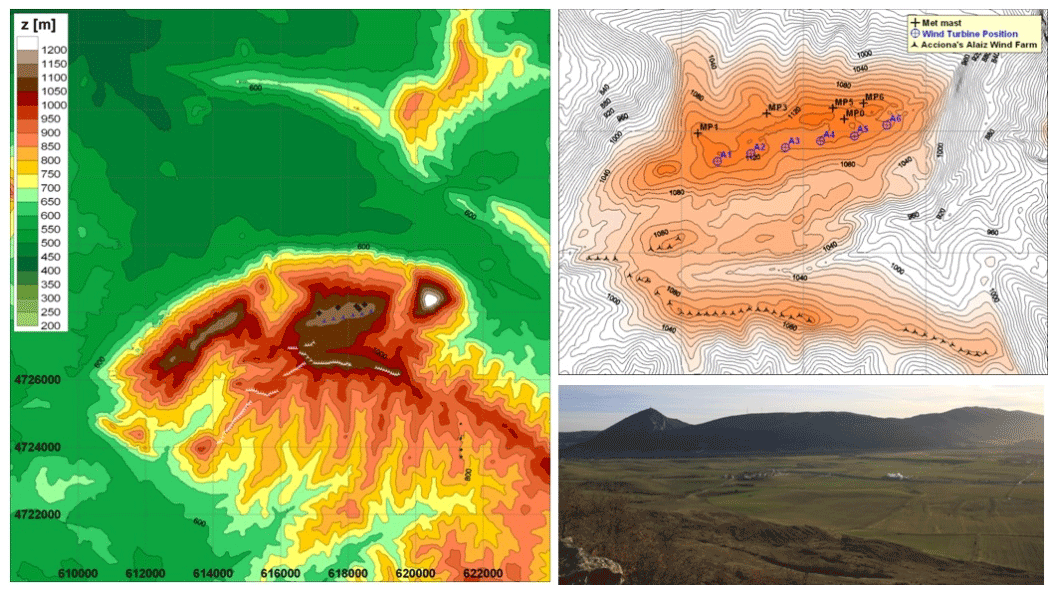
Figure 1 Alaiz elevation map, close-up of the test site and view from the upstream ridge to the north.

Besides the MP5 meteorological mast there are four other reference met masts (MP0, MP1, MP3 and MP6), all of them 118 m tall.

The test site started operating in 2009 with the site calibration procedures. The first wind turbines were installed in the summer of 2011. The standard configuration of each mast is designed for multi-megawatt wind turbine testing and includes sonic and cup anemometer, wind vanes and temperature–humidity measurements. Replicated cup anemometers are situated 2 m below the reference ones.

The MP5 is a permanent 118 m high lattice mast with nine measurement levels with booms oriented to the west (263^∘) and the east (83^∘). Wind speed and wind direction are measured at five levels (118, 102, 90, 78 and 40 m) with a cup anemometer (oriented to the west) and wind vanes (oriented to the east); sonic anemometers are installed at 115.5, 75.5 and 39.5 m (oriented to the west). Temperature and relative humidity are measured at five levels (113, 97, 81, 38 and 2 m) and pressure at 2 m above the ground.

The instrumental set-up is compliant with IEC 61400-12-1 (IEC61400-12-1 (ED1) 2005-12, 2005), with MEASNET cup anemometer calibration (Measnet, 2009) and with ENAC accreditation according to UNE-EN ISO/IEC 17025.

The data acquisition system consists of a real-time controller CompactRIO from National Instruments with 128 MB DRAM and 2 GB storage embedded in a chassis in connection with eight modules of digital and analogical data acquisition, all connected to an Ethernet network.

The rate sample is 5 Hz for the cup anemometer (Vector A100LK) and 20 Hz for the sonic anemometer (METEK USA-1), wind vanes (Thies Compact), pressure sensor (Vaisala PTB100A) and humidity temperature sensor (Ammonit P6312).

Figure 2 Wind rose of 10 min wind speeds observed by MP5 at 118 m for the reference period (July 2014–June 2015).

Figure 2 shows the wind rose at the MP5 site, from the period between July 2014 and June 2015. It presents a bidirectional wind climate, with prevailing winds from the north-northwest sector (330–360, 32 % of total) and the south-southeast sector (150–180, 28 % of total).

4 Methodology

In the present work, a 1-year period (1 July 2014 to 30 June 2015) is analysed. Flux measurements from the sonic anemometer at 115.5, 75.5 and 39.5 m are used to calculate the Obukhov length L, while conventional sensors (wind direction, relative humidity, air pressure and temperature) are used to estimate the bulk Richardson number.

4.1 Data quality control

Before calculating the stability parameter, all data are checked for data quality.

Data from conventional sensors (wind direction, relative humidity, air pressure and temperature) have been processed following Brower (2012). This consists in checking the completeness of the collected data and applying several tests (range, relational and trend). After filtering for quality-control purposes, the conventional sensors provide horizontal wind speed, direction, relative humidity, pressure and temperature availabilities greater than 85 % at all levels during the evaluation period.

For sonic anemometer there are a lot of procedures (Aubinet et al., 2012) and test criteria for quality control of turbulent time series and studies about the impact of these procedures on the results (Stiperski and Rotach, 2015).

High-frequency raw data often contain impulse noise, that is, spikes, dropouts, constant values and noise. Spikes in raw data can be caused by instrumental problems, such as imprecise adjustment of the transducers of ultrasonic anemometer, insufficient electric power supply and electronic noise, as well as water contamination of the transducers, bird droppings, cobwebs, or rain drops and snowflakes in the path of the sonic anemometer.

Several spikes in wind speed have been detected in the raw sonic anemometer data. Therefore, a de-spiking filter is applied based on the change in wind speed from each data point to the next and taking into account the physical limits according to sensor specifications. Data points are removed if they are preceded and followed by changes exceeding the lowest 99 % of all changes. After filtering the spikes, the sonic anemometer provides wind speed and temperature availabilities greater than 80 % in the three sonic anemometers.

4.2 Eddy covariance method

The operating principles of the sonic anemometer are described by different authors (Aubinet et al., 2012; Cuerva et al., 2003; Kaimal and Businger, 1963; Kaimal and Finnigan, 1994; Schotanus et al., 1983). The sonic anemometer output provides three wind components in an orthogonal axis system and sonic temperature. The relation between sonic temperature and absolute real temperature is given by Kaimal and Gaynor (1991).

High-frequency data from sonic anemometer have been processed to obtain 10 min databases that include turbulent fluxes of energy, mass and momentum with the eddy covariance technique (Aubinet et al., 2012; Burba, 2013; Burba and Anderson, 2010; Geissbühler et al., 2000).

The main requirements for instruments and data acquisition systems used for eddy covariance data are their response time to solve fluctuations up to 10 Hz. This means that the sampling frequency has to be high enough to cover the full range of frequencies carrying the turbulent flux, usually leading to a sampling rate of 10–20 Hz. In the test case in this report 20 Hz is the sample rate for the sonic anemometer.

The transformation of high-frequency signals into means, variances and covariances requires different steps (Aubinet et al., 2012; Stiperski and Rotach, 2015); in this study the next steps have been proposed.

1. Quality control of raw data is explained in Sect. 4.1.

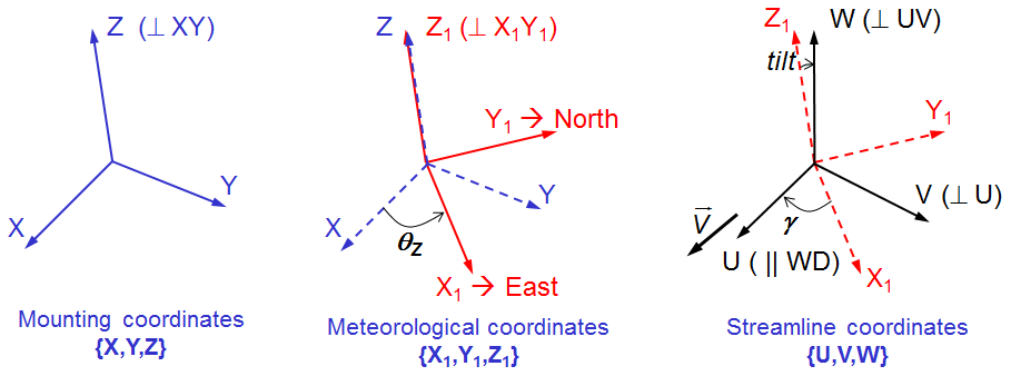
2. Coordinate rotation is the transformation of coordinate systems from the original axes based on the anemometer output to the streamline terrain-following system, based on the planar fit method (PFT) (Richiardone et al., 2008; Wilczak et al., 2001). Momentum fluxes and heat fluxes have been calculated with respect to the streamline terrain-following coordinate system. Figure 3 shows the steps to rotate the axes from mounting coordinates to streamline coordinates.

3. Variance and covariance computation applies the eddy covariance technique for calculation of vertical turbulent fluxes (heat and momentum). It corresponds to the calculation of the covariance of the fluctuations of the vertical velocity with the quantity Φ (temperature for heat, velocity components for momentum).

$$\begin{array}{ll}{\displaystyle }{F}_{\mathit{\varphi }}& {\displaystyle }=\stackrel{\mathrm{‾}}{w^{\prime }{\mathit{\varphi }}^{\prime }}=\stackrel{\mathrm{‾}}{w\mathit{\varphi }}-\stackrel{\mathrm{‾}}{w}\stackrel{\mathrm{‾}}{\mathit{\varphi }}\\ \text{(4)}& {\displaystyle }& {\displaystyle }={\displaystyle \frac{\mathrm{1}}{N-\mathrm{1}}}\left[\sum w^{\prime }{\mathit{\varphi }}^{\prime }-{\displaystyle \frac{\mathrm{1}}{N}}\left(\sum w^{\prime }\right)\left(\sum {\mathit{\varphi }}^{\prime }\right)\right]\end{array}$$

N denotes the number of samples considered for the short averaging period T over which the flux is calculated (from 5 to 60 min). N has to be long enough to ensure statistical convergence and short enough to assume stationarity (in complex terrain difficult to fulfil both criteria). In this work a 10 min averaging period has been selected.

Figure 3 Schematic description for the rotation process.

The MP5's sonic anemometers, at 115.5, 75.5 and 39.5 m height, record temperature, module of the wind speed, wind direction and vertical component (z). These values are projected to meteorological coordinates to obtain the three components of wind speed vector ($x,y,z$). Then, after being filtered, the transformation of high-frequency signals into means, variances, and covariances is done.

The 10 min values of wind speed from the sonic anemometer after applying steps 1 to 3 are checked, and some non-valid data are detected. As in conventional sensors these invalid data are due to icing effects, so they are filtered.

4.3 Stability assessment

The MP5's sonic anemometers allow evaluation of stability based on the local Obukhov length at different heights. This will be the benchmark method since it is directly obtained from the measurements without introducing any assumptions or empirical relationships. The bulk Richardson number is evaluated as an alternative methodology since it follows easier instrumentation set-up and post-processing; for offshore sites it has presented good results (Sanz Rodrigo, 2011; Sanz Rodrigo et al., 2015) and for complex terrain sites it also gives meaningful results (Menke et al., 2019).

4.3.1 Sonic method

To obtain the stability parameter $\mathit{\zeta }=z/L$, as was explained before, sonic anemometer measurements are rotated to the mean streamline coordinate system using the planar fit method to guarantee that the mean streamline plane will be parallel to the terrain surface. After this, variances and covariances of detrended velocity and sonic temperature perturbations are computed using the eddy covariance technique over a high-frequency timescale. Then, turbulent fluxes are obtained by averaging the covariances over a period of 10 min.

In complex terrain, the hypothesis of a homogeneously horizontal surface layer is not fulfilled, so the applicability of Monin and Obukhov similarity theory (MOST) to complex terrain conditions is not obvious. This signifies that for the complex sites such as Alaiz the theory is not completely valid because the topography creates local variations in wind flow near the ground (Kaimal and Finnigan, 1994).

4.3.2 Bulk Richardson number

As was explained before, sonic anemometry is not routinely used in wind energy, and bulk Richardson number Ri_b is an alternative way to estimate atmospheric stability based on a temperature difference and a single velocity level (Eq. 2).

In the Ri_b number equation, potential temperature Θ is the temperature an air parcel with absolute temperature T and pressure p would have if brought adiabatically to the pressure at the 1000 mb level. To the first order it can be calculated as

$$\begin{array}{}\text{(5)}& {\displaystyle }\mathrm{\Theta }=T+\left({\displaystyle \frac{g}{C_p}}\right)\mathrm{\Delta }z.\end{array}$$

Here g is the acceleration due to gravity, $C_p=\mathrm{1000}\mathrm{J}{\mathrm{kg}}^{-\mathrm{1}}{\mathrm{K}}^{-\mathrm{1}}$ is the specific heat capacity of the air at constant pressure and Δz is the height difference from the 1000 mb level.

With Eq. (3) the obtained Ri_b will be used to estimate the stability parameter $\mathit{\zeta }=z/L$. As Bardal et al. (2018) explain, these formulations are only valid for values lower than 0.2, but to make a classification according to atmospheric stability they are considered adequate.

5 Results and discussion

The study is divided into two parts: statistics of atmospheric stability with both methods (the Obukhov length and Richardson bulk) and comparison between both methods.

5.1 Sonic method

Atmospheric boundary layer (ABL) models used in wind farm design tools are typically based on Monin–Obukhov theory. In stable conditions this surface-layer theory is extended to the entire ABL by assuming local scaling of turbulence characteristics through the stability parameter $\mathit{\zeta }=z/L$. This similarity theory would produce self-similar profiles of dimensionless quantities regardless of the height above ground level.

In the study case, as was explained before, from the high-frequency (20 Hz) data recorded in the three available sonic anemometers on the MP5 mast, the values of the Obukhov length (L) over a period of 10 min have been obtained, and taking into account the heights at which they are installed, the parameter $\mathit{\zeta }=z/L$.

In Fig. 4 the stability parameter $\mathit{\zeta }=z/L$ frequency distribution at the three sonic heights is depicted, showing a good agreement among them with a reduction of the percentage of conditions near neutral stability as the measurement height increases. The instantaneous values (10 min), however, do not show good correlation between the different heights (correlation coefficient, R²: 0.25 between 115.5 and 75.5 m, 0.15 between 115.5 and 39.5 m, 0.30 between 75.5 and 39.5 m).

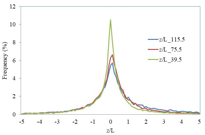
Figure 4 Probability distribution of $z/L$ at all the sonic heights. Only concurrent time steps between July 2014 and June 2015 are included.

Figure 5 shows the distribution of atmospheric stability against wind speed at the MP5 measurement heights. The nine stability classes proposed in Table 1 are reduced to five, combining weakly unstable and stable classes with unstable and stable classes and very unstable and stable with extremely unstable and stable. Table 3 shows the classification used. For the three heights, the stable situations are slightly higher than the unstable ones, and there is an increase in neutral and stable conditions with increasing wind speeds; this is in accordance with the general knowledge that for strong wind speeds the atmosphere becomes neutrally stratified.

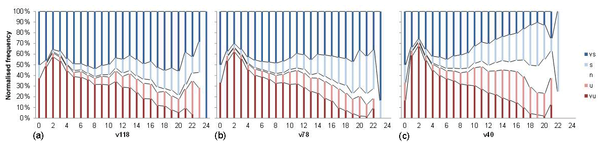
Figure 5 Distribution of atmospheric stability with wind speed based on $z/L$ obtained with the sonic anemometer at different heights: 115.5 m (a), 75.5 m (b) and 39.5 m (c). vs, very stable; s, stable; n, neutral; u, unstable; vu, very unstable.

Table 3 In accordance with Table 1, the five reduced stability classes are shown.

As mentioned before, a significant dependence of stability distributions on height is observed. At higher levels, the stability distributions are broader, and there are more frequent cases with very large and extreme stability. This dependency of the stability distribution with height is because z is part of the definition of the stability parameter, and closer to the ground there are more “neutral” conditions because $z/L$ tends to zero.

The diurnal cycle (see Fig. 6) presents unstable conditions developing from 09:00 to 15:00 UTC. The rest of the day is dominated by stable conditions, resulting in low turbulence intensities.

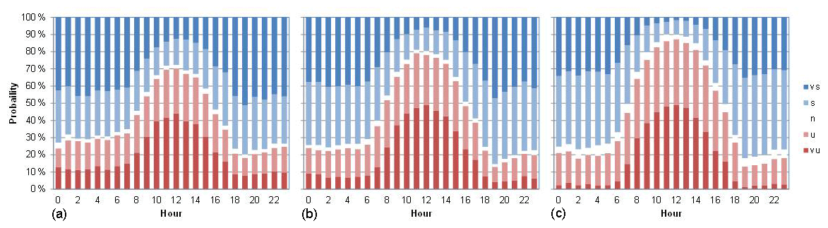
Figure 6 Distribution of atmospheric stability with hour based on $z/L$ obtained with the sonic anemometer at different heights: (a) 115.5 m, (b) 75.5 m and (c) 39.5 m. vs, very stable; s, stable; n, neutral; u, unstable; vu, very unstable.

Figure 7 shows the evolution of stability throughout the year. The stable side dominates during winter months, with unstable conditions peaking between April and August where they take a ≈50 % share.

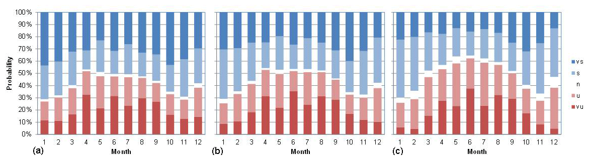
Figure 7 Monthly distribution of stability based on $z/L$ obtained with the sonic anemometer at different heights: (a) 115.5 m, (b) 75.5 m and (c) 39.5 m. vs, very stable; s, stable; n, neutral; u, unstable; vu, very unstable.

The variation in atmospheric stability with wind direction is shown in Fig. 8. Stable situations dominate in most of the directions except for the northwest direction (330–350^∘), which is predominant in Alaiz. As can be seen in Fig. 1, the north face of Alaiz mountain has a steep slope (the roughness index (RIX) value in the north sector of the MP5 position is 22.4 %) that empties into a large valley at around 700 m lower altitude. According to Stull (1989) this topography causes ascending hillside–valley winds that generate convective turbulence and therefore situations of instability that could explain some of the unstable conditions found in the 330–350^∘ direction sector.

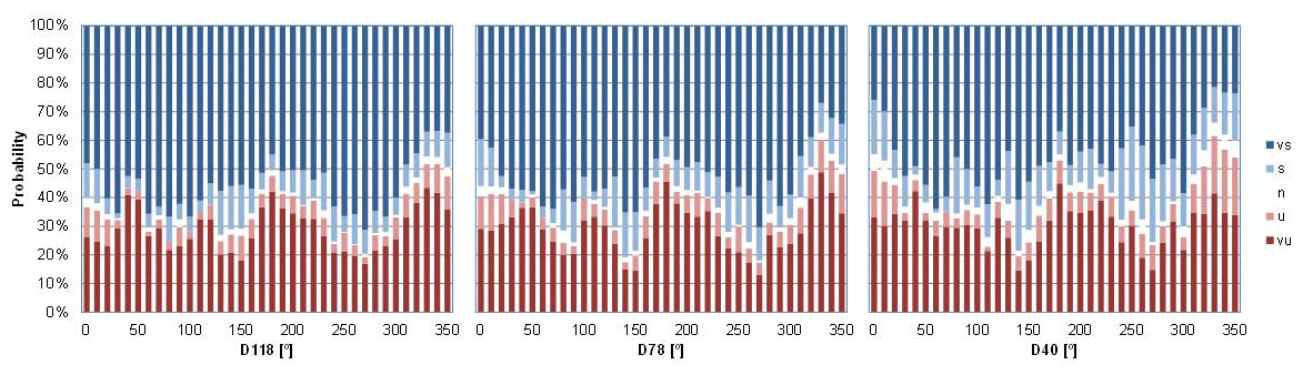
Figure 8 Distribution of atmospheric stability with wind direction based on $z/L$ obtained with the sonic anemometer at different heights. vs, very stable; s, stable; n, neutral; u, unstable; vu, very unstable.

Following the stability classification defined in Table 3, Figs. 9 and 10 present the dependency of wind shear (calculated as the wind speed ratio between 118 and 40 m) and turbulence intensity (calculated as the ratio of the standard deviation to the mean wind speed at 118 m) on stability based on the $z/L$ parameter from the three sonic sensors installed for the NNW and SSE prevailing wind direction sectors.

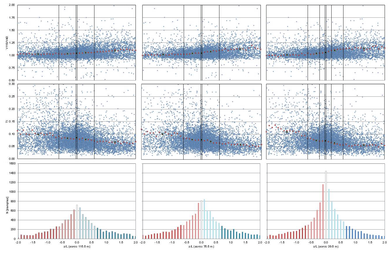
Figure 9 Wind shear and turbulence intensity vs. sonic stability in the MP5 337.5–22.5^∘ sector. Red dots are the $z/L$ mean values for 0.01 resolution scale, and black squares are the $z/L$ mean values in each of the stability classes according to Table 1.

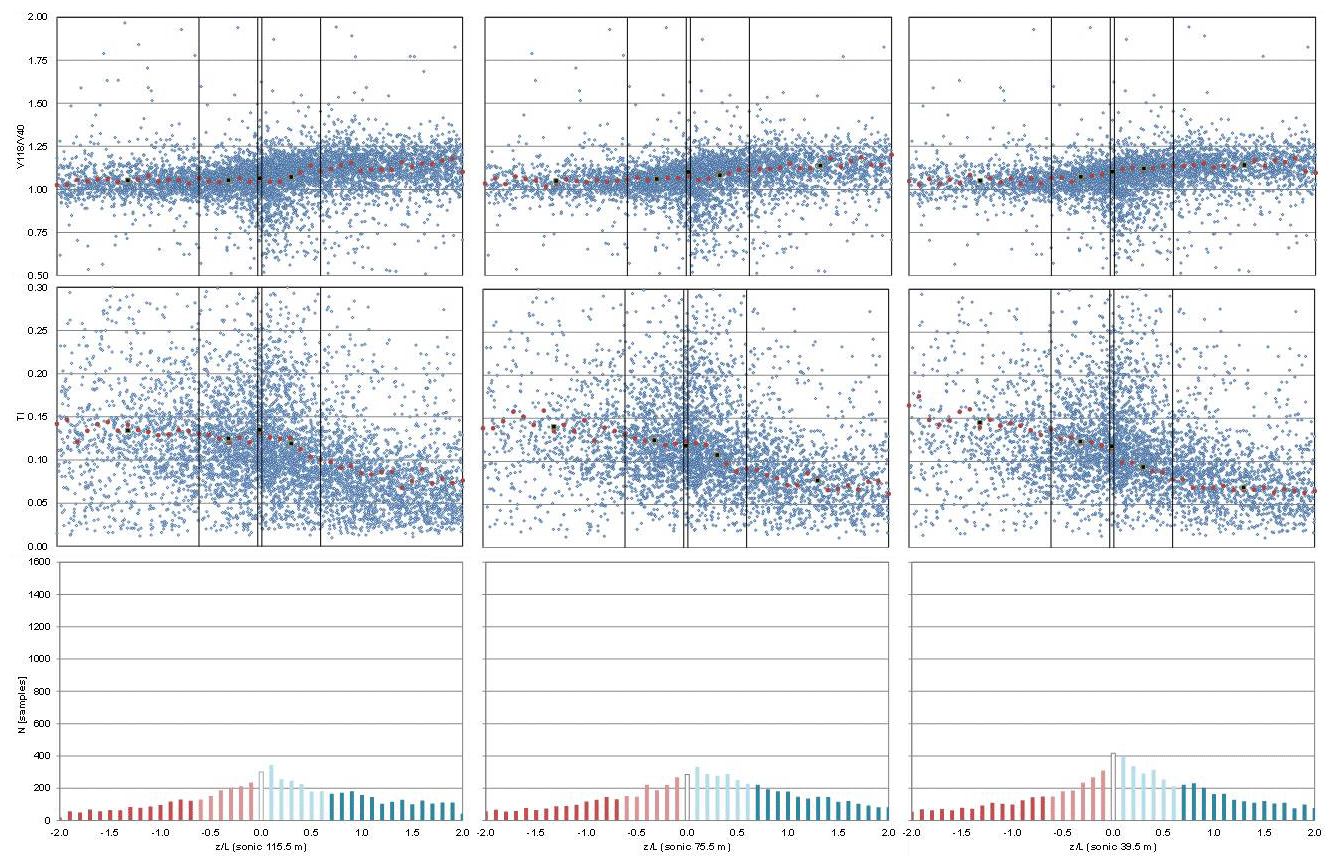
Figure 10 Wind shear and turbulence intensity vs. sonic stability in the MP5 157.5–202.5^∘ sector. Red dots are the $z/L$ mean values for the 0.01 resolution scale, and black squares are the $z/L$ mean values in each of the stability classes according to Table 1.

For the three heights it is observed that, as is explained by Emeis (2013), in unstable situations the ground surface is warmer than the air above so there is a positive heat flux that causes more turbulence. This results in a convective well-mixed surface layer with small vertical gradients. On the other hand, lower turbulence and high shear wind profiles are associated with stable situations where turbulence is reduced due to a negative vertical heat flux.

5.2 Bulk Richardson number

Since sonic anemometers are not commonly used in wind resource assessment, an alternative method to estimate the atmospheric stability is bulk Richardson number. It is based on mean wind speed at height z and mean virtual potential temperature difference between air at the reference height (z) and surface temperature.

The calculation of the bulk Richardson number is, in the present study, not straightforward because of the lack of reliable sensors at the surface. The lower air temperature is measured at 2 m on the MP5 mast. Ideally, the temperature difference at the air–surface interface is required (Kaimal and Finnigan, 1994) for stability analysis. However, because of the lack of surface temperature, 2 m height air temperature has been chosen as representative. Observations of 118 m wind speed and 113 m air temperature have been used in conjunction with 2 m air temperature to estimate Ri_b.

The MP5 mast has no measurements of surface temperature or near the ground. Some authors in these circumstances either extrapolate the values to the surface (z=0) (Machefaux et al., 2016) or perform the calculation directly between the available temperature levels (Martin et al., 2016; Ruisi and Bossanyi, 2019; Zhan et al., 2020). To analyse how the choice of measurement heights may influence resulting Ri_b stability distributions, the Ri_b has also been calculated using 38 m air temperature instead 2 m.

The values of the bulk Richardson number have been obtained over a period of 10 min, i.e. the same period used for calculation of the Obukhov length.

Figure 11 shows the distribution for the bulk Richardson number method. The lower measurement level is varied between 2 and 38 m. Using the 38 m level, it is observed that according to the classification in Table 2, unstable cases practically disappear. This is not physically possible and does not occur in the classification obtained by the sonic method (see Fig. 4). In this case, the results obtained using the 38 m temperature sensor as a representative surface level do not give us any reliable information. Small temperature differences highly affect the result of the Richardson number method, and therefore it is greatly affected by deviations in the measurement of this variable. The MP5 temperature sensors have an accuracy of 0.3 ^∘C, and the mean temperature difference in the period analysed between the level of 38 m and that of 113 m has been 0.7 ^∘C. Thus the uncertainty of the measurement is of the same order as the measurement itself.

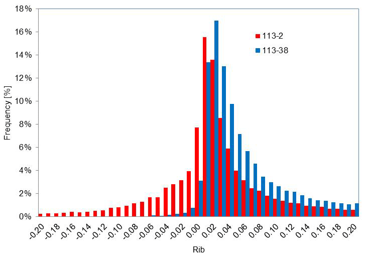
Figure 11 Probability distribution of Ri_b measured between 2 and 113 m (red one) and between 38 and 113 m (blue lines). Only concurrent time steps between July 2014 and June 2015 are included.

The selection of temperature measurement heights has a great effect on the bulk Richardson number method, both in the exactitude and in the applicability of the method. To reduce uncertainties, the measurements should be made either with differential temperature sensors or with calibrated sensors and a sufficient vertical separation in order to reduce the influence of inaccuracies in the temperature measurements (Baker and Bowen, 1989; Brower, 2012).

Figure 12 shows the distribution of atmospheric stability against wind speed. On the left side atmospheric stability is directly classified with the Ri_b obtained with observations of 118 m wind speed, 113 m air temperature and 2 m air temperature; this last temperature sensor has been chosen as representative of surface temperature. The seven stability classes proposed in Table 2 are reduced to five, combining weakly unstable and stable classes with unstable and stable classes. Table 4 shows the classification used. On the right side atmospheric stability is classified according to the stability parameter $\mathit{\zeta }=z/L$ obtained with Ri_b and Eq. (3) and according to the stability classification proposed in Table 3.

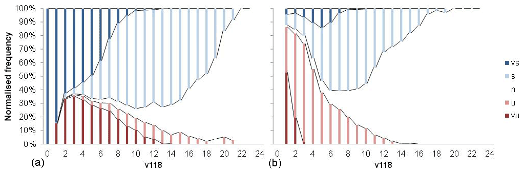
Figure 12 Distribution of atmospheric stability with wind speed (a) based on Ri_b and (b) based on $z/L$ obtained from Ri_b with transformation functions by Businger and Dyer. vs, very stable; s, stable; n, neutral; u, unstable; vu, very unstable.

Table 4 In accordance with Table 2 the five reduced stability classes are shown.

Both distributions show a differentiated behaviour with fewer “very” unstable and stable situations and a greater number of neutral observations in the case of the classification with ζ (on the right side of Fig. 12).

5.3 Comparison of stability methods: sonic versus bulk method

Comparing the distribution of atmospheric stability against wind speed based on the sonic method (Fig. 5) with the results obtained based on the Ri_b method (Fig. 12), it is observed that there are important differences between them.

Table 5 presents a frequency of occurrence of stability classes with concurrent data using different methods. This quantitative comparison shows that taking the sonic method as a benchmark, it is observed that the bulk method, when the Businger and Dyer functions are used to estimate the stability parameter $\mathit{\zeta }=z/L$, overpredict the percentage of neutral and stable conditions to the detriment of very unstable and stable situations, probably due to similar air temperature values at 113 and 2 m. On the other hand, classification directly with rib according to the Mohan classification overpredict the stable situations too at the cost of under-predicting the unstable ones. As is explained in some references (Bardal et al., 2018; Sathe et al., 2011), stability characterisation with Ri_b has several weak points: on one hand the Ri_b method is sensitive to temperature measurements, and uncertainty in L estimation increases as the temperature difference is reduced. In addition, the other source of uncertainty comes from the definition of the surface temperature. On the other hand Businger and Dyer functions have some limitations, and as Bardal et al. (2018) proposed, the use of more advanced methods for relating the Ri_b to the $z/L$ parameter might improve the results.

Table 5 Frequency of occurrence of stability classes.

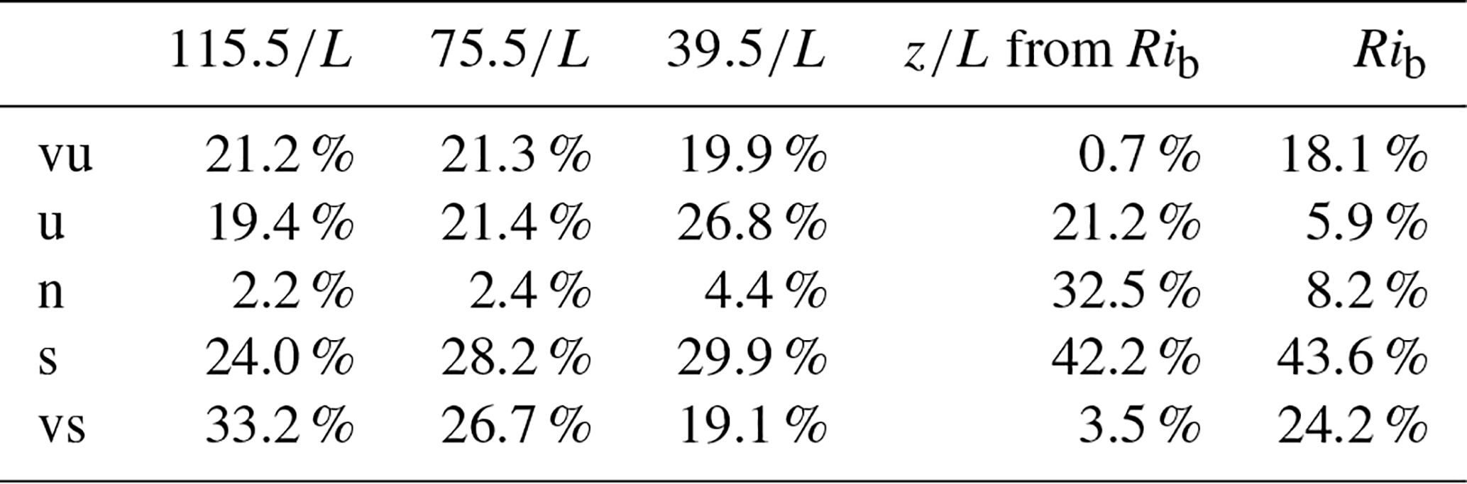
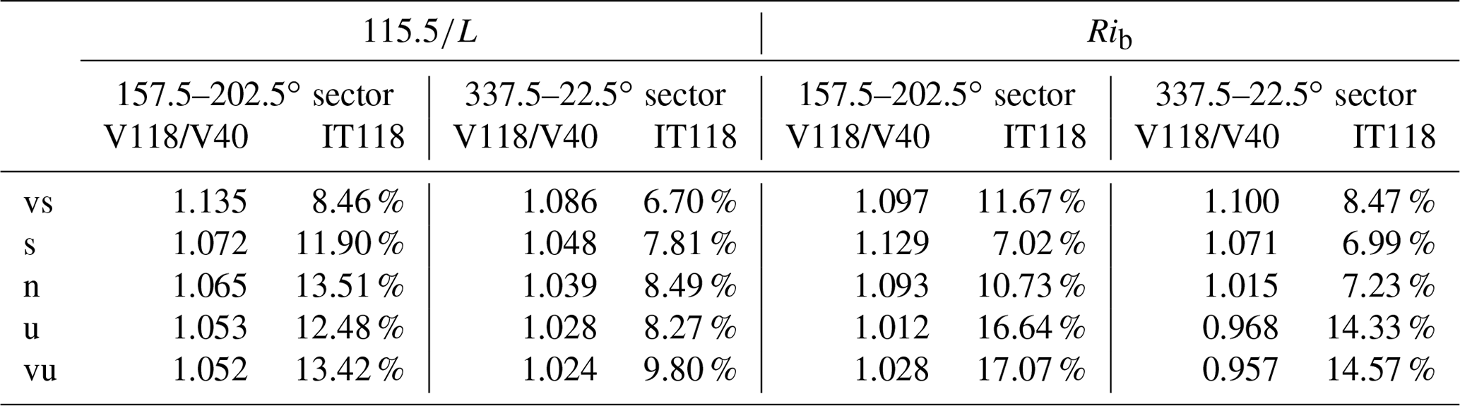
Table 6 Wind shear and turbulence intensity in each of the stability classes. On the left is based on $z/L$, and on the right is based on Ri_b.

Besides these methodological reasons, there are some physical causes of the differences found. One of these is that the Richardson bulk number represents a bulk average stability value instead a local measurement like the sonic method.

As is shown in Table 5, the stability description obtained with the bulk Richardson number does not match the sonic one. The ultimate goal of the stability characterisation is to provide good predictive power of turbulence intensity and shear at hub height. Thus in order to analyse it, Table 6 shows these values in each of the stability classes with both methods in the two main wind direction sectors in MP5. In comparison with the sonic method, the stability characterisation with the bulk Richardson number underestimates the wind shear (overestimating the turbulence intensity) for unstable situations in both sectors. For neutral and stable situations it depends on the wind sector.

6 Conclusions

In this work, a detailed data analysis focuses on how to estimate atmospheric stability at a site with complex terrain. The Obukhov parameter $\mathit{\zeta }=z/L$, which can be measured locally with the use of a sonic anemometer, and bulk Richardson number have been studied. The methods are examined considering their theoretical background, implementation complexity, instrumentation requirements and practical use in connection with wind energy applications.

It is shown that the resulting stability depends on which method is chosen. The sonic method is taken as a benchmark because it is the only way of measuring local stability without the use of empirical functions or theoretical assumptions. However, this method requires working with accurate high-frequency data, rotating the measurements to align the coordinate system to the mean wind vector, which is reported to require special attention in complex terrain to guarantee that the mean streamline plane will be parallel to the terrain surface, to finally obtain turbulent fluxes using the eddy covariance technique.

According to the stability parameter $\mathit{\zeta }=z/L$ obtained with the three sonic anemometers installed on the MP5 mast, for the three heights, the stable situations are slightly higher than the unstable ones, and there is an increase in neutral and stable conditions with increasing wind speeds. There is a significant dependence of stability distributions on height. At higher levels, the stability distributions are broader, and there are more frequent cases with very large and extreme stability.

The seasonal and diurnal cycle is identified: in the winter and during the hours between 17:00 and 8:00 UTC the stable side dominates, while between April and August and between 9:00 and 15:00 UTC unstable conditions are found to be more frequent. Winds from the predominant northwest direction (330–350^∘) produce more unstable conditions than the other sectors.

For the three heights, and in the two predominant sectors, it is observed that in unstable situations the ground surface is warmer than the air above, so there is a positive heat flux that causes more turbulence. This results in a convective well-mixed surface layer with small vertical gradients. On the other hand, lower turbulence and high-shear wind profiles are associated with stable situations where turbulence is reduced due to a negative vertical heat flux.

As an alternative to characterise stability, the bulk Richardson number is explored, which requires a minimum level of instrumentation, mean wind speed at height z and mean virtual potential temperature difference between air at the reference height (z) and surface temperature. The bulk Richardson number can be used directly to classify the atmospheric stability, or it can be transformed into $\mathit{\zeta }=z/L$ by Businger and Dyer functions.

On the MP5 there is not a surface temperature sensor, so the 2 m air temperature sensor has been chosen as representative. Moreover, to analyse how the choice of measurement heights may influence resulting Ri_b stability distributions, it has also been calculated using a 38 m air temperature sensor instead of 2 m. This configuration does not give us any reliable information, which could be due to temperature sensors on the MP5 having an accuracy of 0.3 ^∘C. The mean temperature difference in the period analysed between the level of 38 m and that of 113 m has also been 0.7 ^∘C, so the uncertainty of the measurement is of the same order as the measurement itself. The Ri_b number relies on smaller temperature differences for estimation of the mean gradient, and its accuracy is therefore dependent on the sensor precision, calibration and measurement heights. The following recommendations are provided to obtain consistent results with the bulk Richardson method: use high-precision temperature sensors, calibrate all the temperature sensors at the same time, calibrate the temperature sensors in the operational range to guarantee better calibration in the temperatures of interest and have a reference temperature sensor below 2 m, as close to the ground as possible. On the other hand, the stability classification obtained directly using the Ri_b values shows a differentiated behaviour than that estimated according to the stability parameter $\mathit{\zeta }=z/L$ obtained with Ri_b and Businger and Dyer functions. This differentiated behaviour could be the different classification employed in characterisation (Mohan vs. Sorbjan and Grachev) and/or by the Businger and Dyer functions.

In summary the sonic method is more costly and complex, but, in this study, it shows results in accordance with the general atmospheric boundary layer knowledge, so we recommend it as a first option to obtain a local measurement of atmospheric stability that can be associated with a certain height above the ground and in consequence provide good predictive power of turbulence intensity and wind shear at hub height. For the bulk Richardson number, based in the references read, there is not a standard methodology for characterising atmospheric stability using this method, and there are many different approximations. Furthermore, empirical relations to relate Ri_b to $\mathit{\zeta }=z/L$ are obtained either for offshore sites or for non-complex sites, so there is a need for observational studies on complex terrain to increase understanding of how to estimate atmospheric stability accurately with the bulk Richardson number.