A multipurpose lifting-line flow solver for arbitrary wind energy concepts

In this work, we extend the AeroDyn module of OpenFAST to support arbitrary collections of wings, rotors, and towers. The new standalone AeroDyn driver supports arbitrary motions of the lifting surfaces and complex turbulent inflows. Aerodynamics and inflow are assembled into one module that can be readily coupled with an elastic solver. We describe the features and updates necessary for the implementation of the new AeroDyn driver. We present different case studies of the driver to illustrate its application to concepts such as multirotors, kites, or vertical-axis wind turbines. We perform verification and validation of some of the new features using the following test cases: elliptical wings, horizontal-axis wind turbines, and 2D and 3D vertical-axis wind turbines. The wind turbine simulations are compared to existing tools and field measurements. We use this opportunity to describe some limitations of current models and to highlight areas that we think should be the focus of future research in wind turbine aerodynamics.

1 Introduction

Horizontal-axis wind turbines (HAWTs) have been the mainstream focus of the wind energy community in the past few decades, and most aerodynamic tools are centered around such a concept. For example, this is the case for the multiphysics solver OpenFAST (Jonkman et al., 2022) developed by the National Renewable Energy Laboratory. The OpenFAST solver is dedicated to HAWTs and cannot¹ study other wind energy concepts, such as vertical-axis wind turbines (VAWTs), kites, airborne wind energy concepts, and arbitrary assemblies of rotors and blades/wings. This article attempts to bridge this gap by focusing on new aerodynamic functionalities to the aerodynamic model of OpenFAST, named AeroDyn. This first step can be followed later by extending the structural dynamics modules to accommodate these different concepts.

The most common method for the study of a HAWT is the blade element momentum (BEM) method (Glauert, 1935). The method cannot be applied to other concepts, though it inspired the development of streamtube models for VAWTs (Strickland, 1975; De Vries, 1979; Paraschivoiu and Delclaux, 1983). General purpose computational fluid dynamics (CFD) solvers are commercially available and have been applied to various wind energy concepts (Makridis and Chick, 2013; Folkersma et al., 2017; Rezaeiha et al., 2017). Their use by the wind energy community is still limited, and dedicated solvers are typically preferred. Such solvers (e.g., Ellipsys, Sørensen, 1995; FLOWer, Weihing et al., 2018; and ExaWind, Sprague et al., 2020) have generic grid-based implementations, but they have been primarily applied to HAWTs. However, simulations of alternative wind energy concepts using these solvers are emerging in the literature (Bangga et al., 2020). CFD applications with arbitrary motions are still challenging and not readily available. Vorticity-based methods have long been considered the intermediate solution between the computationally intensive CFD methods and the engineering models, such as BEM (Perez-Becker et al., 2020; Boorsma et al., 2020). Panel-based and lifting-line methods are readily applied to arbitrary assemblies of wings and rotors (Katz and Plotkin, 2001). The open-source code QBlade (Marten et al., 2013) contains a generic vorticity-based solver that has been applied to HAWTs (Saverin et al., 2018a) and VAWTs (Saverin et al., 2018b). Other generic solvers have been implemented (van Garrel, 2003; Chatelain et al., 2013; Branlard et al., 2015; Alvarez and Ning, 2019; Boorsma et al., 2020) but not often publicly distributed.

In this work, we leverage the recent implementation of the open-source lifting-line vortex code, OLAF (cOnvecting LAgrangian Filaments), integrated in AeroDyn (Shaler et al., 2020) and present verification and validation of this tool. We extend the AeroDyn module to support arbitrary collections of wings, rotors, and towers. Assemblies of rotors can be handled with BEM or OLAF, while more complex geometries are handled with OLAF only. The existing driver for AeroDyn is also extended to support arbitrary geometries, provide functionalities to prescribe arbitrary motions to the lifting surfaces, and prescribe complex turbulent inflows. In this work, we combined the aerodynamic and inflow modules into a standalone module so that it can readily be coupled with structural solvers, paving the way for aeroelastic simulations of arbitrary wind energy concepts.

In Sect. 2, we describe the features of the new AeroDyn driver and the updates to the AeroDyn modules and briefly mention the implementation. In Sect. 3, we present different applications of the driver and perform verification and validation of some of its features. We use this opportunity to describe some limitations of current models and highlight areas that we think should be the focus of future research in wind turbine aerodynamics. We conclude our work by summarizing these research questions and providing paths for future work.

2 Features and implementation

In this section, we describe the main features of the newly implemented AeroDyn driver. The original AeroDyn driver was limited to the simulation of HAWTs, with a fixed nacelle position, and inflows limited to a power-law shear profile (more advanced structural motions and wind conditions can be simulated when coupling AeroDyn within OpenFAST, including aeroelastic effects and turbulence). To model advanced wind energy concepts, the driver was augmented to model rotors and wings of arbitrary geometry, undergoing arbitrary rigid-body motion and under arbitrary inflows. As such, the driver can be used for configurations that are not currently supported by OpenFAST. To facilitate the future coupling with a structural solver, we combined the aerodynamic and inflow modules into a new module. The features of this driver include the following.

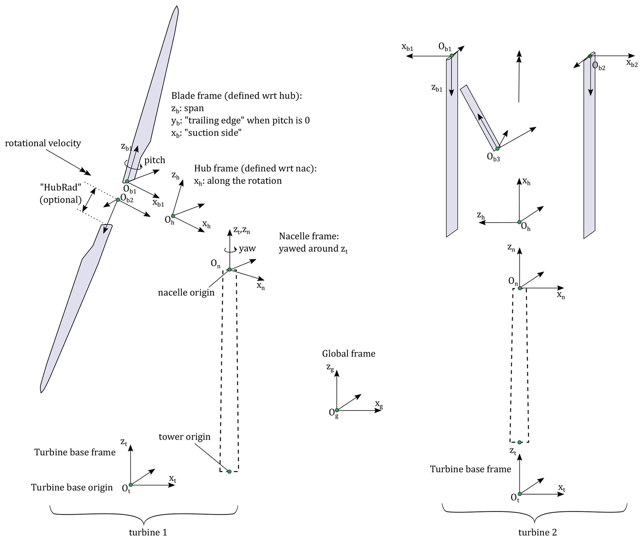
Figure 1 Definition of frames and origins for a two-turbine configuration – HAWT (left) and VAWT (right).

• Inflow. The wind field may be defined in three ways: (1) using a uniform power law, (2) using a time-varying power law (where both the reference velocity and the power-law coefficient change with time), or (3) using any wind supported by the InflowWind module (Jonkman et al., 2022) – uniform steady wind, unsteady wind speed and direction (e.g., deterministic gusts), and turbulent wind field of various file formats.

• Geometry. An assembly of fixed or rotating blades/wings is called a “turbine.” The driver can have an arbitrary number of turbines. Each turbine comprises one optional tower and a set of blades. Several bladeless turbines consisting of a single tower can be used to model structures made of multiple towers. An example of a configuration with two turbines is shown in Fig. 1. The figure defines the different frames used for each turbine – the turbine base frame (labeled, t), the nacelle frame (n), the hub frame (h), and the blade frames (b). The labels are used to identify the frame axes and the origins in the following. As indicated in Fig. 1, the coordinate systems must be such that the hub rotation occurs about the x_h axis, and the blade frame must be such that x_b and y_b point toward the suction side and the trailing edge, respectively, when the pitch and twist angles are zero. The turbine base and tower base have distinct origins, but they share the same frame. The tower top is assumed to coincide with the nacelle origin. The origins and orientations of each frame are input by the user, where coordinates are given relative to the parent frame, and orientations are given using the values of three successive rotations (x–y–z Euler angle sequence) taken from the parent frame. A user switch is available to facilitate the input of generic HAWT geometries. In this framework, an arbitrary wing is set up as a turbine with no rotational speed and an optional tower.

• Motion. Motion inputs are provided independently for the base, nacelle, hub, and blades of each turbine. The base motion may be fixed, sinusoidal in one of six degrees of freedom, or arbitrary. The arbitrary motion is provided using time series of time, three translations, three successive rotations, three translation velocities, three rotational velocities, three translational accelerations, and three rotational accelerations. The nacelle yaws around the z_n axis, and the user may fix the yaw angle or provide a time series of the nacelle yaw angle, speed, and acceleration. The rotor rotates about the x_h axis, and the user may specify a constant rotational speed or a time-varying time series (angular position, speed, and acceleration). Blade pitching occurs around the individual z_b axes. The user can specify constant pitch or time series of pitch (position, speed, and acceleration) for each individual blade. Nonrotary wings are considered a special case with 0 rotational speed. The different rigid-body motions are easily implemented using the mesh-mapping routines of OpenFAST, called within the AeroDyn driver.

• Flow solver. The driver operates with AeroDyn, and the different wake options of AeroDyn can be used to solve the flow. The options currently available are no induction (using the geometric angle of attack), quasi-steady and dynamic BEM for HAWTs (Moriarty and Hansen, 2005; Branlard, 2017), or the vortex wake code, OLAF (Shaler et al., 2020). AeroDyn is currently being extended to support hydrokinetic turbines (including buoyancy and added mass effects); future implementations will include a double-streamtube momentum model for VAWTs. Currently, BEM and OLAF cannot be used simultaneously, but such options will be considered in the future.

• Analysis types. Different analysis types are provided by the driver. In particular, parametric studies can be run by providing a table of combined-case analyses. Refer to the OpenFAST manual for additional details (Jonkman et al., 2022).

• Outputs. The driver outputs time series of motion, loads, and aerodynamic variables to individual files for each turbine. Additionally, 3D visualization outputs are available for the individual bodies. When OLAF is used, Lagrangian markers and velocity–vorticity planes can be output to visualize the wake.

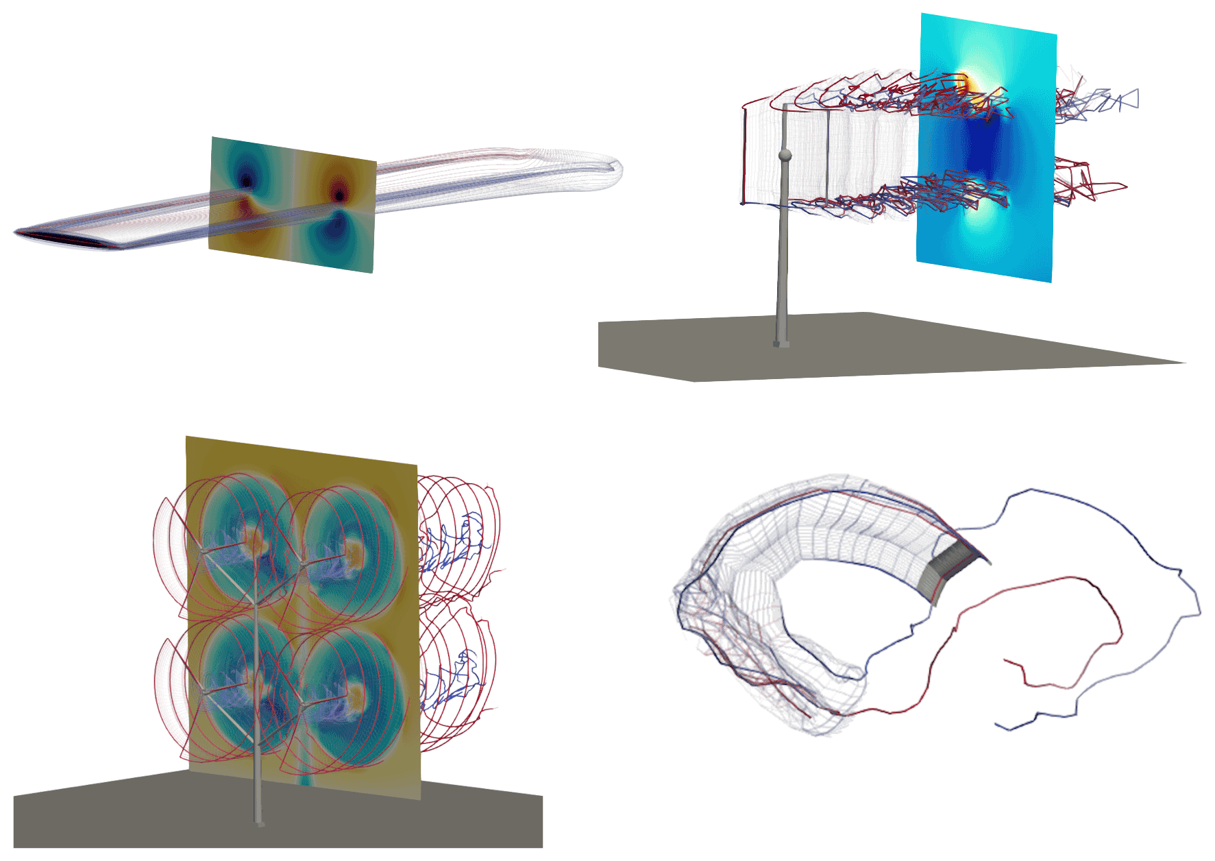
Figure 2 Example of wind energy concepts to which the AeroDyn driver may be applied – (clockwise from top left) elliptical wing, VAWT, kites, and multiple rotors.

Changes to the AeroDyn module consisted of supporting multiple rotors throughout the code, with different parameters for each rotor, and extending OLAF so that it can handle an assembly of wings with different numbers of input sections. In this work, we added two dynamic stall models to AeroDyn – the Boeing Vertol (BV) model (also present in CACTUS; Murray and Barone, 2011) and the dynamic stall model of Øye (Øye, 1991; Branlard, 2017). Both models are documented in the OpenFAST documentation (Jonkman et al., 2022). The driver was fully rewritten to accommodate the new features and to couple with the new module that combines aerodynamic and inflow. The source code of the AeroDyn driver is open source and available on the OpenFAST repository (Jonkman et al., 2022), together with its documentation. Example input files, including some of the cases presented below, are also available and integrated as part of the OpenFAST testing framework.

3 Results: verification, validation, and path forward

3.1 Illustrative examples

We begin this section by showing visual outputs from simulations done using the AeroDyn driver applied to different wind energy concepts. OLAF was used for all simulations because it can be applied to arbitrary geometries, and it offers an opportunity to visualize the wake. Visualizations of the wake, blades, towers, and velocity planes are shown in Fig. 2 for an elliptical wing, a VAWT, a kite performing a “figure eight,” and a “quad-rotor” with multiple towers. In the remaining portion of this section, we will look at specific applications to verify and validate the current implementation. Each investigation will point to research topics for future work on the aerodynamics of wind energy concepts. These points will be summarized in the conclusion.

3.2 Elliptical wing and HAWT – effect of regularization

3.2.1 Elliptical wing

In this section, we use the elliptical wing test case presented by van Garrel (2003) to illustrate the capability of the AeroDyn driver in studying isolated lifting lines (not necessarily rotors). The wingspan is b=5 m; the chord $c=c_{\mathrm{0}}\sqrt{\mathrm{1}-(\mathrm{2}y/b{)}^{\mathrm{2}}}$, where c₀=1 m; and the n+1 panel nodes are located via a cosine distribution at the spanwise coordinates $y=b/\mathrm{2}\cos \mathit{\theta }$, with θ spanning linearly from −π to π. The control points are located between the panel nodes, according to the cosine-approximation algorithm of van Garrel. The wind speed is 1 m s⁻¹ in the chordwise direction and 0.1 m s⁻¹ normal to the chord, leading to a geometrical angle of attack of 5.7106^∘. The profile data are uniform along the wingspan and set with a linear lift coefficient: C_l(α)=2πα. The wake convects with the free stream only (no rollup). We use three different numbers of panels for the verification: $n=[\mathrm{20},\mathrm{40},\mathrm{80}]$. The baseline results, similar to van Garrel's study, are those without regularization (no “vortex core”), indicated by a zero value of the regularization parameter ϵ. We demonstrate the impact of the regularization by performing simulations with n=80, with a regularization parameter proportional to the chord (ϵ=0.5c) or with a constant parameter (ϵ=0.1). We use a Lamb–Oseen regularization kernel as a multiplicative factor to remove the singularity; the regularization parameter is the same for the wing and the near-wake panel, and it is constant throughout the wake. The lift coefficient along the span is shown in Fig. 3. It was obtained using OLAF coupled with the AeroDyn driver. The vortex wake results extracted from van Garrel's report are also provided in the figure. The strong agreement between the two vortex wake codes supports the verification of OLAF's implementation. Both lifting-line implementations are expected to rely on the same formulation. The results from AeroDyn are reported at the panel nodes and not the control point nodes of OLAF, explaining the minor differences observed toward the wing tips for n=20. Under the linear and classical lifting-line approximation of Prandtl (Katz and Plotkin, 2001; Branlard, 2017), the theoretical lift coefficient for the wing is $C_{\text{L,th}}=\mathrm{2}\mathit{\pi }\mathit{\alpha }[\mathrm{1}+\mathrm{2}/\text{AR}{]}^{-\mathrm{1}}\approx \mathrm{0.47653}$, where $\text{AR}=b^{\mathrm{2}}/(\mathit{\pi }b{c}_{\mathrm{0}}/\mathrm{4})$ is the wing aspect ratio. The theoretical value is indicated on the figure. The current simulation setup (cosine distribution without regularization and wake rollup) is well suited to approximate the linear theory but is not expected to match the results fully. To match the linear theory, linear assumptions are needed, and the wake needs to follow the chord instead of the free stream. Requirements to match the theory exactly are provided in Chapter 3 of Branlard (2017). The impact of the regularization is clearly observed in Fig. 3, and the choice of the regularization parameter can have a drastic impact on the results.

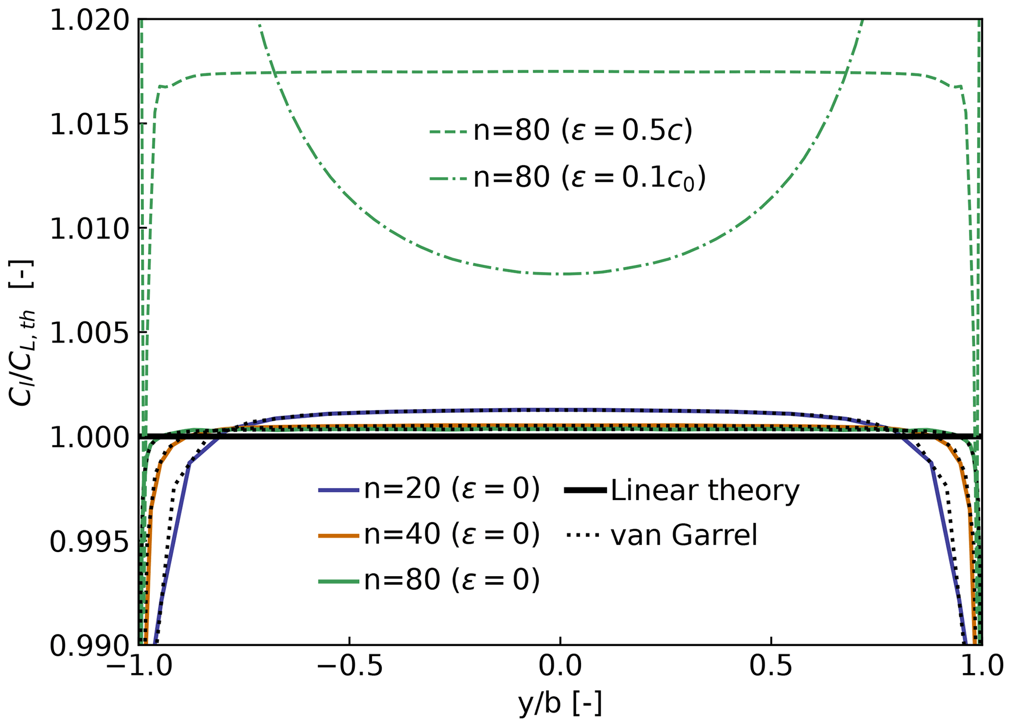
Figure 3 Lift coefficient along elliptical wing (C_l) as predicted by two similar lifting-line implementations (OLAF and van Garrel) and the linear lifting-line theory (C_L,th). Results for various numbers of spanwise stations (n) and regularization parameters (ϵ).

3.2.2 HAWT

To illustrate the impact for a HAWT, we use the Big Adaptive Rotor (Bortolotti et al., 2021) operating at a tip-speed ratio of λ=8, with a thrust coefficient of C_T=0.64 and a power coefficient of C_P=0.46.

In the plot on the left in Fig. 4, we show the different regularization parameter distributions used, normalized by the maximum chord of the turbine. The regularization parameter is proportional either to the chord or to the spanwise discretization (here, the spanwise discretization is constant). We plot the resulting axial and tangential induction factors along the blade on the middle and right in Fig. 4. We observe that the regularization parameter influences the induction at the tip, middle, and root of the blades, where circulation gradients are the strongest. A large value of the regularization factor leads to smoother, more regular induced velocity distributions, whereas lower values allow for more sudden changes. In this particular example, we observed (results not included here) differences in normal and tangential loads of up to 6 % and 30 %, respectively, within the first 40 % span of the blade and differences up to 2 % and 8 % toward the tip of the blade. The power and thrust coefficients vary up to 2.3 % and 0.7 %, respectively. Both variables tend to take larger values with increased values of the regularization parameter.

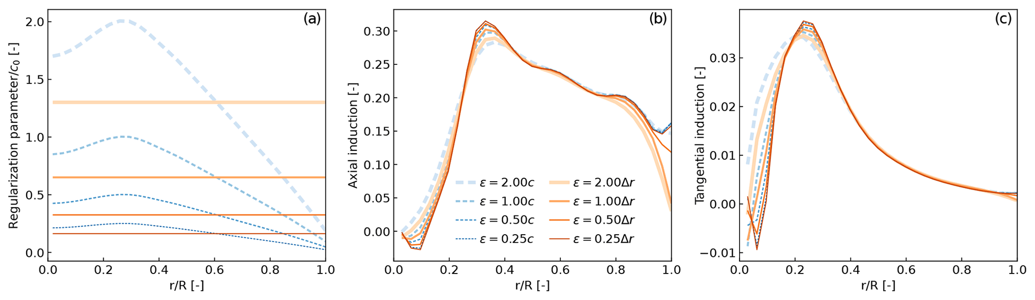
Figure 4 Influence of the regularization parameter on the induction factors obtained along a wind turbine blade. (a) Regularization parameter normalized by maximum chord. (b) Axial induction. (c) Tangential induction.

3.2.3 Discussion on regularization

We observed a strong dependence of the flow quantities on the lifting line with respect to the regularization parameter. We expect that the regularization parameter should be characteristic of the physical size of the bound vorticity to obtain a realistic simulation of a wing or a turbine blade. This physical size is related to the size of the boundary layer (Branlard, 2017), which is often proportional to the chord. As we observed, results will also be a function of the spanwise discretization. Vortex methods require the size of the regularization parameter to be proportional to the grid size for the method to converge to the Euler or Navier–Stokes equations (Cottet and Koumoutsakos, 2000). Therefore, physical and numerical regularizations operate differently, and we expect that a reformulation of the lifting-line algorithm itself is necessary to ensure convergence of the method. Additionally, vortex methods introduce more scales as the temporal and spatial discretization is refined. The regularization in the wake is essential to filter some of these new scales introduced. An adequate and physical filtering may be achieved using subgrid scale models and proper account of viscous diffusion – but such models are not readily available for a filament-based vortex method and are hard to achieve unless the topology and connectivity of the wake are modified. The topic of regularization is being actively researched for actuator line CFD (Martínez-Tossas and Meneveau, 2019; Meyer Forsting et al., 2019) and vortex-based methods (Li et al., 2020). Future work should focus on the convergence of the lifting-line method with blade discretization and convergence of the filament-based vortex method, through comparisons with measurements and blade-resolved simulations.

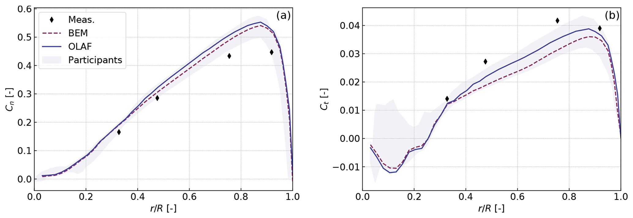
Figure 5 Simulation of a HAWT using the AeroDyn driver. Results for test case IV.1.2 (constant, uniform inflow) of IEA Task 29. Normal and tangential force coefficients along the blade span (respectively a and b).

3.3 HAWT – comparison with BEM

AeroDyn was previously dedicated to HAWTs, and its BEM implementation was extensively tested for such configurations. In this section, we present comparisons between BEM, OLAF, and measurements for the three-bladed NEG-Micon NM80 turbine, rated at 2 MW, with a rotor diameter of 80 m. Details about the turbine and the experimental setup are available in the DanAero report (Madsen et al., 2010). We use the test cases from the International Energy Agency (IEA) Wind Task 29 as validation cases (Schepers et al., 2021). In this work, we present results using the AeroDyn driver for a rigid rotor. Results using OpenFAST for a flexible rotor are provided in the IEA Wind Task 29 report, together with a full description of the IEA Wind Task 29 test cases and results from other participants. For the cases presented below, flexibility effects were found to have a negligible impact on results.

3.3.1 Uniform inflow

We begin with case IV.1.2 from the IEA Wind Task 29. The rotor operates at a tip-speed ratio of λ=8.5 for an average wind speed of U₀=6.1 m s⁻¹. The test case neglects shear, and constant uniform inflow is assumed for the simulations. The force coefficients normal and tangential to the chord line are shown in Fig. 5. The coefficients were obtained by normalizing the forces with $\mathrm{1}/\mathrm{2}\mathit{\pi }\mathit{\rho }{U}_{\mathrm{0}}^{\mathrm{2}}R$, where R is the rotor radius and ρ is the air density. The simulation results shown in Fig. 5 are consistent with results obtained by other institutions (Schepers et al., 2021), for both the BEM and vortex code. The comparison with measurements is fair but leaves room for improvement. We discuss these results further in Sect. 3.3.3.

3.3.2 Sheared and yawed inflow

We use cases IV.2.1 and IV.2.2 to study the aerodynamics in sheared and yawed conditions, respectively. Both cases have the same rotational speed and pitch; the tip-speed ratios are 6.9 and 8.0, respectively; the yaw angles are 6 and 38^∘, respectively; and the power-law exponents are 0.25 and 0.26, respectively. We model the tower shadow effect using the potential flow model of OpenFAST. Figure 6 presents the results for both cases as a function of the azimuthal position. We interpolated the normal loads and tangential loads radially to obtain them at the radial positions of the measurements: $r/R=[\mathrm{0.33},\mathrm{0.48},\mathrm{0.75},\mathrm{0.92}]$. The azimuth is 0 when the blade is pointing up and 180 when passing the tower, where the tower shadow model effect is visible. We performed elastic (with ElastoDyn) and rigid (with AeroDyn driver) simulations. We observe some differences between the two (comparing dashed and plain lines of the same color), but these differences are not as pronounced as the differences between BEM and OLAF (comparing blue and red curves). The vortex code agrees significantly better with the measurements than the BEM method for the yawed case. The shear-only case appears to be challenging, especially at 33 % and 48 % span, where the behavior captured by the codes is opposite to what is observed in the measurements.

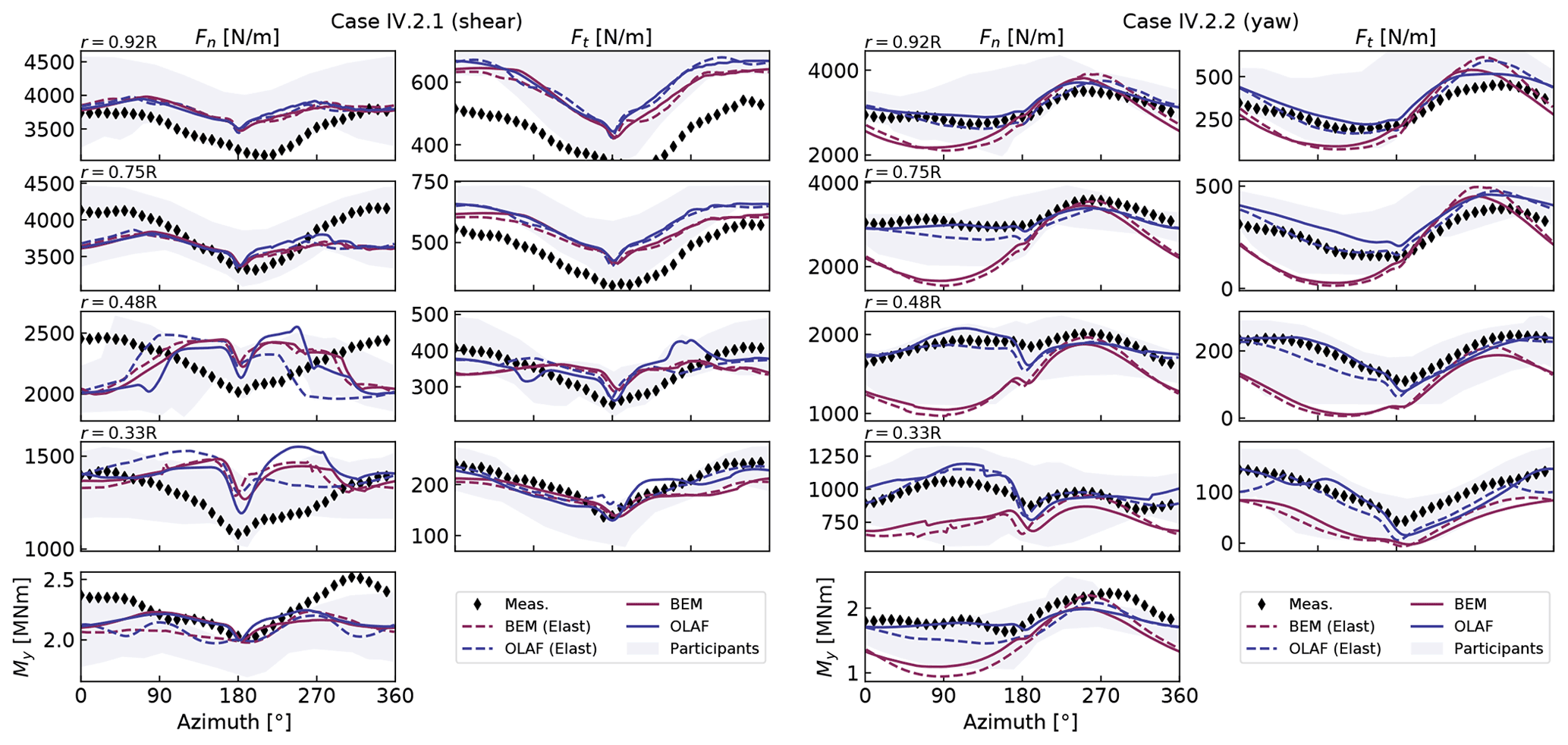
Figure 6 Results for a HAWT (NM 80) under strong shear (left) and yawed (right) conditions. The normal (F_n) and tangential (F_t) loads are shown at four radial positions as a function of the azimuth. The blade root flapping moment, M_y, is shown at the bottom. Elastic (“Elast”) and rigid simulations are compared to the DanAero measurements.

3.3.3 Discussion on the results

Despite the simplicity of the uniform inflow case, we observed some differences between the BEM and vortex methods in the results presented in Fig. 5. The differences are attributed to the fact that the rotor is at a moderately high load as well as to fundamental differences in the formulation. BEM assumes the blade annuli to be independent, does not inherently account for out-of-plane effects such as prebend, and relies on empirical corrections. In this simulation, the average induction factor is 0.4, corresponding to a moderately high loading case where a high-thrust correction is needed in BEM. Segment-based vortex methods are of higher-level fidelity, but they suffer from the issue of regularization mentioned in Sect. 3.2. The mean relative errors in axial inductions and angle of attack are 4 % between the two methods. The mean relative error of the tangential induction is around 20 %, and the error in normal and tangential forces is 3 % and 6 %, respectively. The differences between BEM and vortex methods are in line with results from other participants.

The discrepancies between BEM and OLAF observed in the yaw case (Fig. 6) indicate that the implementation of the yaw model in AeroDyn may need further improvements. It is possible that BEM implementation changes, such as those presented by Branlard et al. (2014) or Perez-Becker et al. (2020), could improve the results. Nevertheless, reasons for such discrepancies will require further investigation.

The differences observed between measurements and simulations in Figs. 5 and 6 were primarily attributed to the definition of the polar data used by the lifting-line codes in the IEA report (Schepers et al., 2021). In general, the CFD-based method performed better than the lifting-line methods. Therefore, we expect an improvement of results using an updated set of polars.

3.4 VAWT

3.4.1 2D case

In this section, we use the 2D VAWT model presented by Ferreira et al. (2014): a two-bladed turbine of radius R=1 m, with blades of constant chord c=0.1 m and 15 % relative thickness. The lift coefficient is set to C_l=2π1.11sin α, and the drag and moment coefficients are zero. The tip-speed ratio is λ=4.5. Simulations were run using the vortex code CACTUS (Murray and Barone, 2011), and with OLAF, and compared with the double-multiple streamtube model (DMST) results that we extracted from the figure of Ferreira et al. (2014). The angle of attack as a function of azimuth is shown in Fig. 7. The differences between the vortex code results and the DMST are similar to what was observed and discussed by Ferreira et al. (2014). The vortex codes CACTUS and OLAF are observed to strongly agree in this case for the estimation of the angle of attack. CACTUS uses a vortex formulation where the velocity at control points is obtained from the average of the velocity at the nodes and where the wake is being shed at the lifting line. The original OLAF formulation uses the induced velocity obtained in between nodes and sheds the wake at the trailing edge of the blade. For this work, OLAF was modified to have a similar formulation as CACTUS. In the case presented in Fig. 7, we observe that by using the same formulation (i.e., comparing CACTUS and OLAF “CP+Wake“ in the figure), a slightly better agreement is obtained. A more significant impact of the implementation was observed on other simulations. Some authors argue that unsteady effects are better captured when the shedding of vorticity occurs at the trailing edge or a quarter chord behind the trailing edge (Katz and Plotkin, 2001). Such conclusions are likely to be true for panel methods but might not apply for lifting-line methods. In light of the current results, it appears that this choice of implementation for VAWTs (shedding at trailing edge, location of control points) may still be an open question.

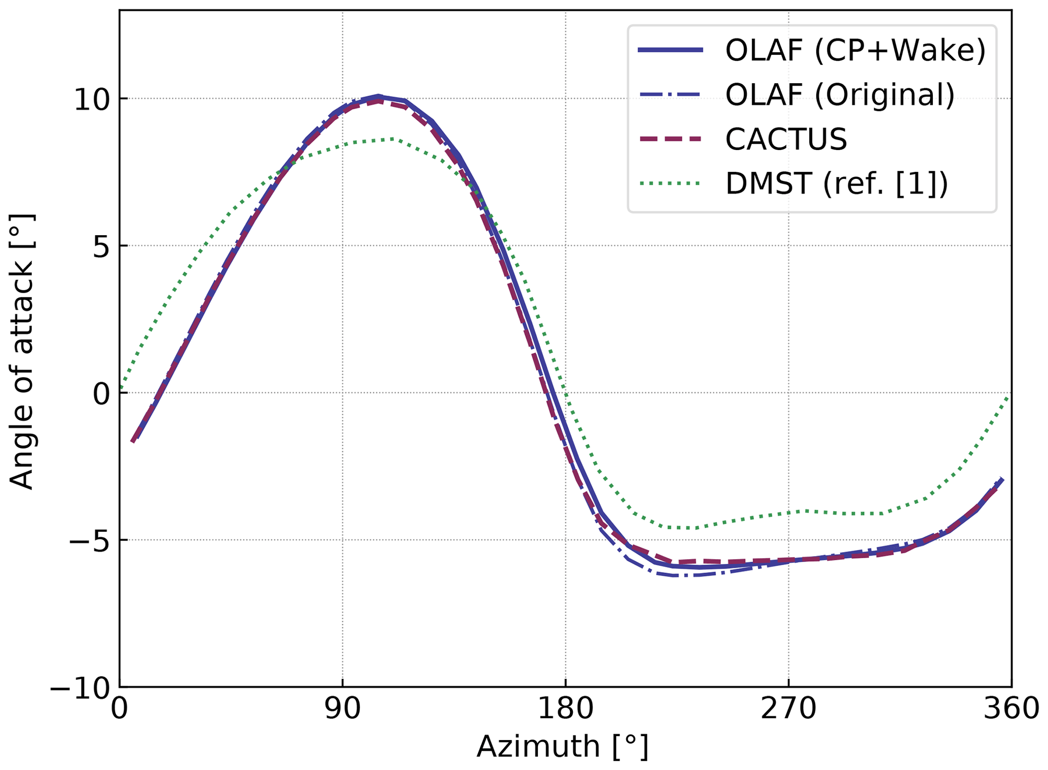
Figure 7 Angle of attack on a 2D VAWT as obtained with various vortex methods and with the double-multiple streamtube (DMST) theory.

The previous test case does not activate the dynamic stall model² as a result of the low angle of attack and artificial lift coefficient used. We replaced the polar data with realistic polar data of a NACA0015 airfoil that stalls at approximately 8.5^∘. The angle of attack is similar to the one obtained in Fig. 7, oscillating between ±10^∘, but the dynamic stall has a strong influence on the lift coefficient and power coefficient. In this work, we implemented the BV model and the dynamic stall model of Øye. AeroDyn also includes three variations of the Beddoes–Leishman (BL) model (Leishman and Beddoes, 1989): the Gonzalez (BL Gonz.) and Minemma/Pierce (BL MP) variants (Damiani and Hayman, 2019) and the four-state model from Hansen et al. (2004) (BL HGM). The impact of the choice of the dynamic stall on the power coefficient is shown in Fig. 8 for a simulation at λ=4.5. From the figure, it is observed that the choice of dynamic stall model has a dramatic impact on the aerodynamic performance. It is common practice in the VAWT community to tune the parameters of the dynamic stall model such as to achieve performances that match the measurements. To illustrate this, we increased the stall angle parameter of the BV model by 1^∘ (labeled “BV α+1” in the figure). Again, such a change has a strong impact on the response, delaying the onset and activation of the dynamic model. It is clear how such tuning of the coefficients can lead to desired responses and performances. Overall, the spread of results indicates that dynamic stall models for VAWTs (and, likely, HAWTs) should be the topic of future research.

Figure 8 Influence of the choice of dynamic stall model on the power coefficient of a 2D VAWT.

3.4.2 3D case – comparison with measurements

In this section, we model a prototype 5 kW VAWT with the new AeroDyn driver. The turbine consists of nine blades – three vertical blades, each attached to the hub by two support arms. A picture of the wind turbine is shown in Fig. 9. The turbine was designed and constructed by XFlow Energy and was tested at the Field Laboratory for Optimized Wind Energy (FLOWE) in Lancaster, California. The turbine was tested between February and April 2020. The field measurements were collected using two six-axis load cells mounted between the vertical blades and its support arms. The load cells were custom units developed by Sensing Systems from Dartmouth, Massachusetts. The wind speed was measured using a pair of APRS #40R anemometers, positioned 2 rotor diameters upstream of the rotor. The measurements presented have had inertial effects subtracted.

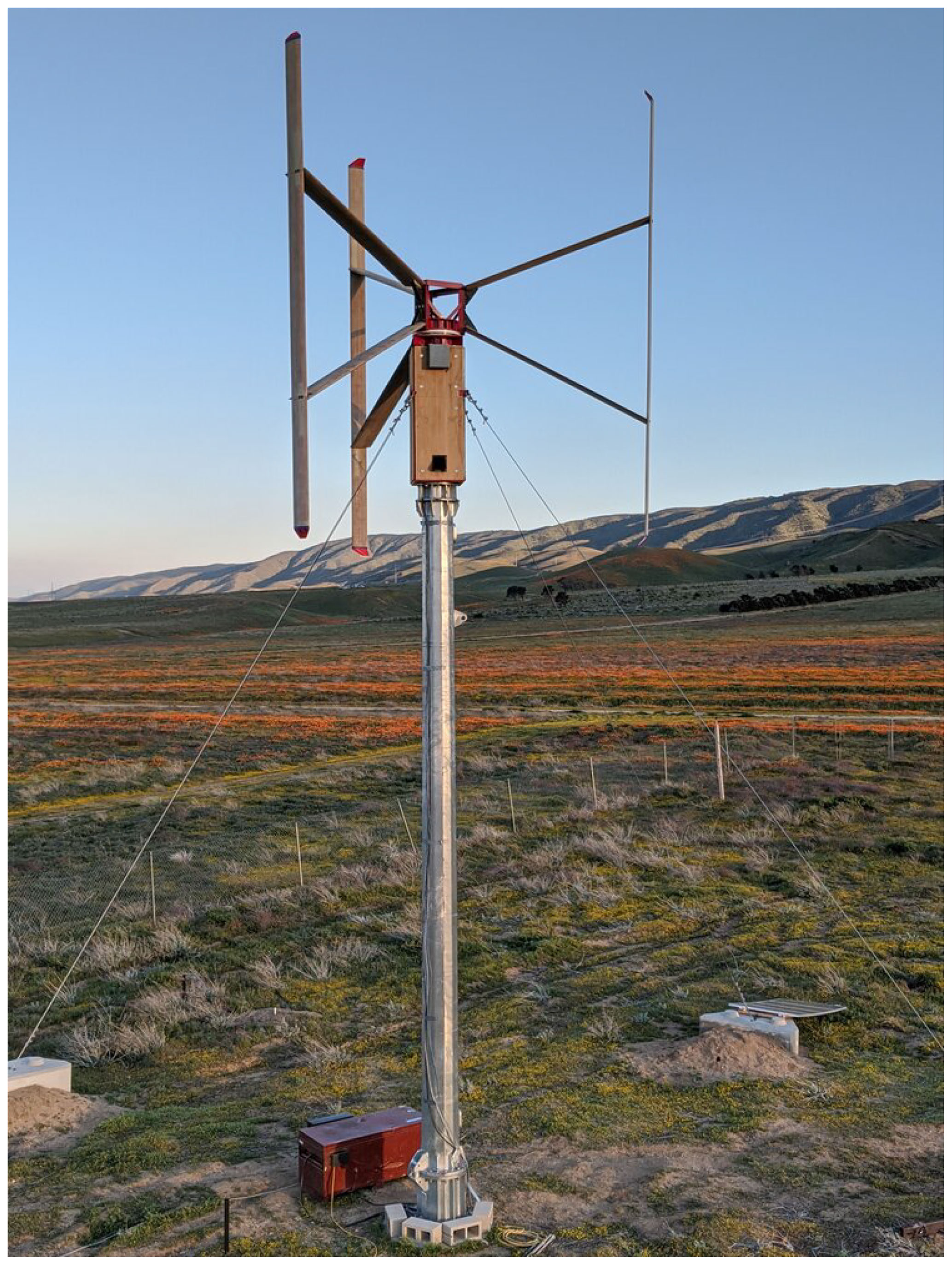
Figure 9 XFlow's 5 kW prototype VAWT at the Field Laboratory for Optimized Wind Energy in Lancaster, California.

First, we run simulations with steady inflow and constant rotational speed to evaluate the power curve of the turbine. The power coefficient as a function of tip-speed ratio is compared to field measurements in Fig. 10. We used two different sets of inputs for these simulations: the first one favors CACTUS, whereas the second set favors OLAF. In the first set, the dynamic stall coefficients of the BV model were tuned such that the CACTUS simulation would match the measured power curve, and the excrescences (drag losses associated with connections, bolts, etc.) were computed as an additional loss term:

$$\begin{array}{}\text{(1)}& {\displaystyle }{C}_{\mathrm{P}}=C_{\text{P,clean}}-\mathrm{\Omega }{\displaystyle \frac{\left[C_{Q,\text{exc}}{Q}_{\mathrm{0}}\right]}{P_{\mathrm{0}}}},\end{array}$$

where C_P,clean is the power coefficient obtained from the vortex code with clean polars, P₀ is the reference power (typically $P_{\mathrm{0}}=\mathrm{1}/\mathrm{2}\mathit{\rho }A{U}_{\mathrm{0}}^{\mathrm{3}}$, with A the swept area), Q₀ is the reference torque (typically $Q_{\mathrm{0}}=\mathrm{1}/\mathrm{2}\mathit{\rho }{R}^{\mathrm{3}}(\mathrm{\Omega }R{)}^{\mathrm{2}}$, though the definition may differ), and the term in brackets is the excrescences torque, which is further defined in Murray and Barone (2011). The excrescences torque coefficient was evaluated by computing the difference between the experimental and CACTUS-simulated torque for a case where the turbine rotation is prescribed but the inflow is zero, giving $C_{Q,\text{exc}}=\mathrm{0.009}$. In the second method, we performed a joint optimization of the drag polars and the dynamic stall parameters such that the OLAF results would match the power curve measured in the field. In this second case, the excrescences were directly accounted for by the increased drag in the polar data, which was expected to be more realistic. In Fig. 10, the results labeled “OLAF 1, clean” are results from the first set of inputs, without the excrescences and with the clean polars. The labels “1” and “2” indicate which sets of input are used. We observe in Fig. 10 that both vortex codes capture the main characteristics of the power curve.

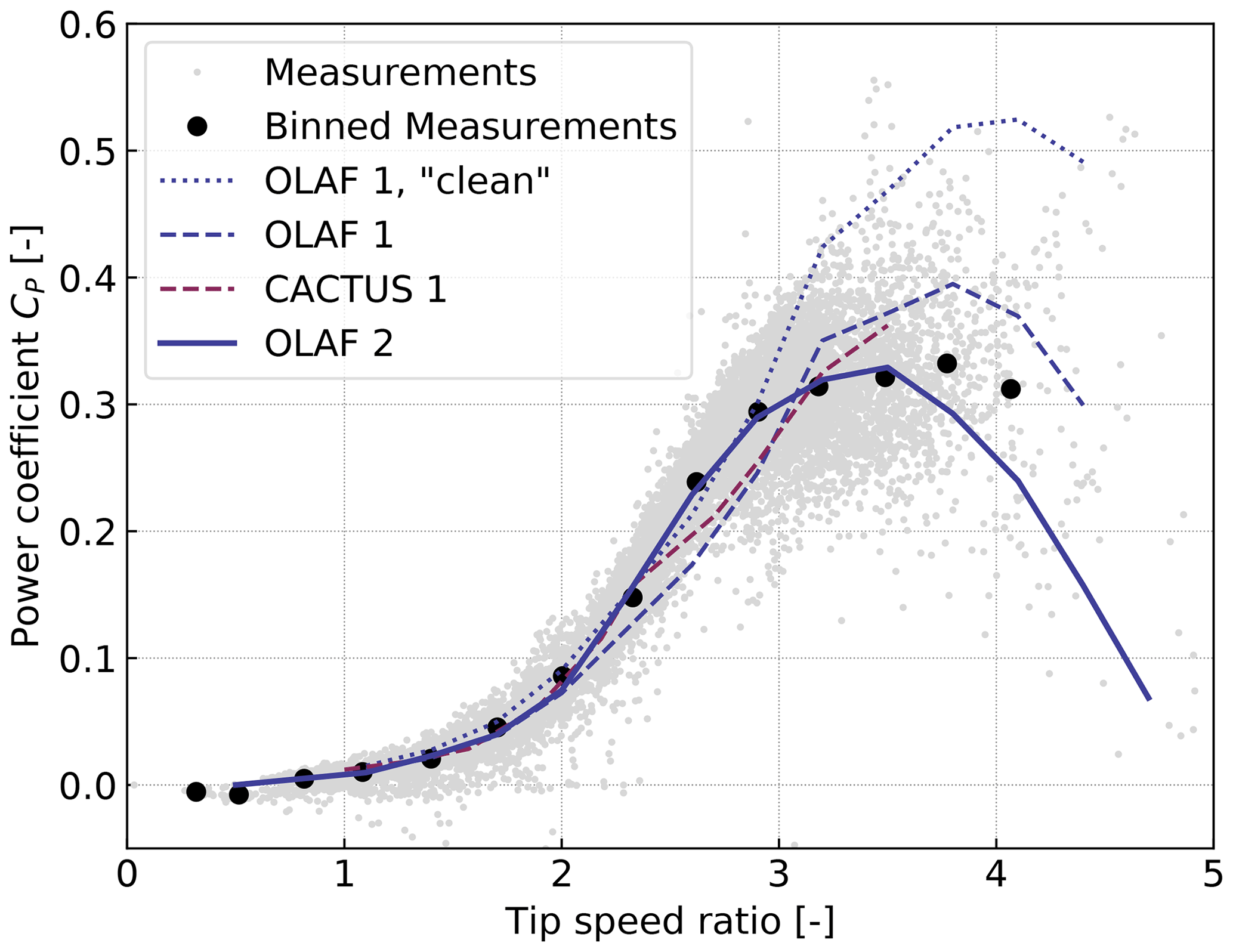
Figure 10 Performance of the VAWT model as obtained with the simulation tools OLAF and CACTUS, compared with measurements for two sets of inputs (one tuned for CACTUS, another tuned for OLAF). The curve “OLAF 1, clean” does not include excrescences.

Despite a similar implementation used between OLAF and CACTUS, some differences of outputs for this advanced structure are observed. For the first set of results (tuned for CACTUS), the performances obtained using OLAF appear to be under-predicted below λ=3 and over-predicted otherwise, indicating that the difference in implementation can have an important impact on the predictions. The second set of results shows that OLAF can capture the experimental power curve using a different tuning of the dynamic stall coefficients. This second set of results also illustrates that a tuning of the drag coefficient is possible to account for excrescences instead of adding a constant torque.

We illustrate the differences between the models by looking at time traces of the total force on the first vertical blade at different tip-speed ratios. Dimensionless force coefficients are computed as $C=F/(\mathrm{1}/\mathrm{2}\mathit{\rho }(\mathrm{2}R{)}^{\mathrm{2}}{U}_{\mathrm{0}}^{\mathrm{2}})$, where F is the force in a given direction. The forces are reported in the coordinate of the blade (described in Fig. 1). The force coefficients obtained from field measurements and simulation are compared in Fig. 11. To demonstrate the capabilities of the AeroDyn driver, simulations with shear and turbulence were also carried out. The power-law profiles and turbulence intensities from the field measurements were used to generate synthetic turbulent inflow with TurbSim (Jonkman and Buhl, 2006). Results from these simulations, averaged over 24 revolutions, are indicated by the label “OLAF (turb)” in Fig. 11. The azimuthal positions 90 and 270^∘ correspond to the positions where the blade is upwind and downwind, respectively. A fair agreement with the measurements is obtained for both tools. The response when the blade is in the wake (270^∘) appears more challenging to capture, in particular at higher tip-speed ratios and for the tangential coefficient (C_y). This likely indicates issues related to the estimation of the drag force or the account of viscous effects in the wake. In general, a strong agreement is observed between OLAF and CACTUS. Spikes observed in the CACTUS simulations are not present in the OLAF runs, which display a smoother response. The differences between the turbulent and uniform simulations appear to be minor but are expected to become more important for larger shear and turbulence intensities.

Figure 11 Force coefficients as measured and simulated on the VAWT model.

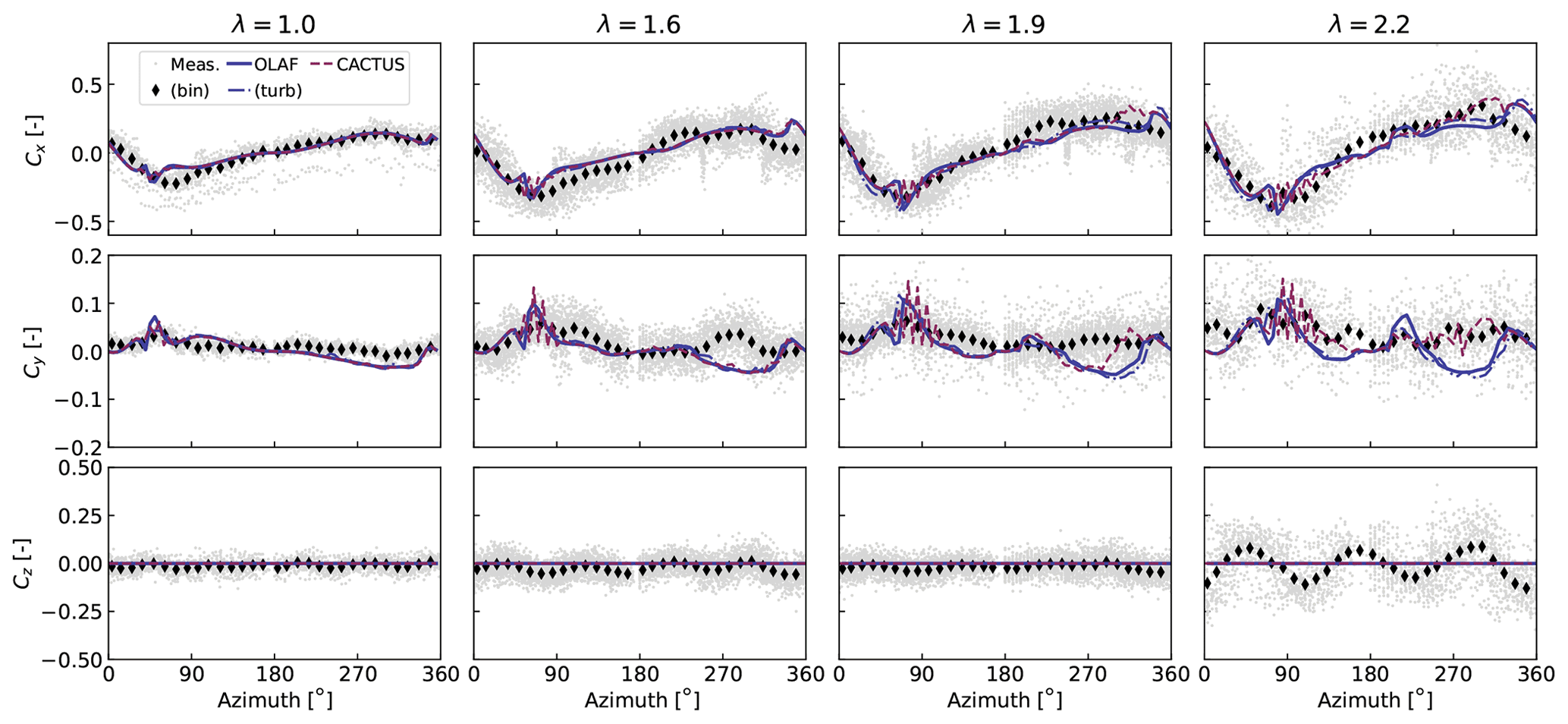
Based on a finite element analysis of XFlow's 5 kW turbine geometry, we expect C_x to be the least affected by aeroelastic effects. This agrees well with the simulation and is a possible explanation for discrepancies observed in the simulated C_y and C_z compared to the field results. Based on the finite element analyses, the turbine's first mode of excitation corresponds to a vertical motion of the blades, which is observed to be a dominant effect in the field measurements. Because of this, it is not surprising that the rigid-body AeroDyn/OLAF simulations did not capture the oscillations observed in C_z. Future work coupling OLAF with an elastic solver should more accurately capture this effect.

3.5 Discussions on vertical axis simulations with vortex methods

In this section, we presented examples of simulations of 2D and 3D VAWTs, verified them using other simulation tools, and validated them against measurements.

By diving into the implementation details of CACTUS, we found some differences of formulation, which can explain the differences observed between the two simulation codes. Some of the differences between OLAF and CACTUS include the presence (or absence) of a “trailing-edge” vortex, the location of the control points (on the nodes or in between them), and the location of the points used for the determination of the angle of attack (CACTUS uses points at the one-fourth, one-half, and three-fourths chord for the BV model). Additional features were implemented in OLAF, and it is now possible to switch between these formulations to better match the CACTUS implementation. Additional work is needed to determine which formulation is the most accurate.

The current approach for VAWT modelers consists of tuning the dynamic stall parameters to obtain performances that match the measured ones. We applied this approach in this work to illustrate that the method can indeed be used successfully. Nevertheless, the approach cannot be considered satisfactory, and the large spread of results that we obtained in Fig. 8 for different dynamic stall models indicates that more research is needed on the topic. In particular, future work should focus on deep stall and large fluctuations of angle of attack, which are relevant for VAWTs.

We found that when the turbine passes its own wake, the simulated loads were in noticeable discrepancy with the field measurements. The reasons for such differences are currently not well understood. They may be related to regularization issues and, potentially, the lack of vorticity shedding when the blade is stalling. It is also possible that the blade–vortex interaction is not well captured by the lifting-line vortex method. Flow field measurements focusing on the wake and its interaction with the blade may help answer this question.

4 Conclusions

In this work, we described the features of a general-purpose driver to perform aerodynamic simulations of wind energy concepts. We demonstrated different applications to highlight the versatility of the new driver. In most applications, we used the vortex code OLAF, and we presented verifications and validations of this newly implemented code. Throughout the article, we pointed to different areas for future research, namely the following.

• We showed that the regularization parameter of lifting-line vortex methods, commonly referred to as the vortex core, has a strong impact on the accuracy of the lifting-line quantities and should be further investigated. Measurement and blade-resolved CFD can be used as a reference, providing detailed load distributions along the blades and flow fields of the wake. The lifting-line method should be improved to ensure convergence as the spanwise discretization is increased, while preserving a physical size of the regularization parameter and, therefore, ensuring that physical flow fields are obtained near the blade and in the wake. Filament-based vortex methods should also display convergence in the wake for increased spanwise and temporal resolutions. Such convergence might require the implementation of dedicated viscous and subgrid-scale models.

• We found that different lifting-line vortex code implementations can lead to different loads and induction fields, depending on the choice of formulation. Some of the differences between OLAF and CACTUS include the presence (or absence) of a trailing-edge vortex, the location of the control points (on the nodes or in between them), and the angles of attack used in dynamic stall models. Some of CACTUS formulations were implemented in OLAF. Additional work is needed to determine which formulation is the most accurate.

• Using the IEA Wind Task 29 test cases, we observed that the BEM theory is challenged by out-of-plane situations (yaw, shear, and coning), and, despite the ad hoc corrections available, the method does not capture all the trends observed in measurements. Using OLAF showed a substantial improvement in the yawed test case; therefore, future work will be dedicated to improving the yaw model of AeroDyn.

• The choice of dynamic stall model significantly impacts the simulation results of VAWTs. Practitioners commonly fall back to tuning the parameters of the model because we lack a universal and reliable model. More research is needed on the topic; specifically, focusing on deep stall and large fluctuations of angle of attack, which are relevant for VAWTs.

• We noted that for VAWTs, the differences between measured and simulated loads were noticeable when the blade passes in the wake. We hypothesized that this could be due to a poor capture of the blade–vortex interaction or a flawed representation of the wake due to nonphysical regularization, or due to a lack of vorticity shedding when the profiles are in stall.

Aerodynamic concepts different from the widely studied HAWTs offer a variety of aerodynamic challenges. The new aerodynamic driver opens the door for further investigation of these concepts. Targeted aerodynamic studies within a controlled environment can be carried out using the new prescribed motion feature. The feature is relevant for future aerodynamic research areas, including floating offshore wind turbines or unsteady aerodynamics effects under (prescribed) elastic motions (e.g., flutter). The aerodynamic models currently implemented in AeroDyn consist of the BEM method (both quasi-steady and dynamic) and a lifting-line vortex lattice solver. AeroDyn will soon be extended to support hydrokinetic turbines. Additional models will be added in the future, such as the double-multiple streamtube model and mixed formulations between BEM and vortex methods.