Influence of wind turbine design parameters on linearized physics-based models in OpenFAST

While most physics involved in wind energy are nonlinear, linearization of the underlying nonlinear wind system equations is often important for understanding the system response and exploiting well-established methods and tools for analyzing linear systems. Linearized models are important for eigenanalysis (to derive structural natural frequencies, damping ratios, and mode shapes), controls design (based on linear state-space models), etc. In controls co-design, wherein methods often rely on linearized time-domain models of the physics, the physical structure (often called the plant) and controller are designed and optimized concurrently, so it is important to understand how changes to the physical design affect the linearized system. This work summarizes efforts done to understand the impact of design parameter variations in the physical system (e.g., mass, stiffness, geometry, and aerodynamic and hydrodynamic coefficients) on the linearized system using OpenFAST.

1 Introduction

The Aerodynamic Turbines Lighter and Afloat with Nautical Technologies and Integrated Servo-control (ATLANTIS) program funded by the US Department of Energy (DOE) Advanced Research Projects Agency-Energy (ARPA-E) seeks to develop new technology pathways for the design of economically competitive floating offshore wind turbines (FOWTs) based on controls co-design (CCD) principles. Within ATLANTIS Topic Area 2 (Computer Tools), the National Renewable Energy Laboratory (NREL) leads a project developing the Wind Energy with Integrated Servo-control (WEIS) toolset, which is new independent software that combines Wind-Plant Integrated System Design & Engineering Model (WISDEM^®), OpenFAST (formerly known as FAST), and CCD functionality together with the goal of providing the offshore wind energy industry and research communities with an open-source, user-friendly, flexible tool to enable true CCD of the FOWT physical design together with the controller (Jonkman et al., 2021).

CCD methods, including those being implemented within WEIS, often rely on linearized time-domain models of the physics (e.g., an optimal open-loop controller is solved with direct transcription based on a linearized time-domain model using quadratic programming, from which an optimal closed-loop controller can be derived for use in a higher-fidelity nonlinear time-domain analysis). Here, the open-loop controller is optimized concurrently with the physical design (plant) via either a nested or simultaneous approach (Herber and Allison, 2019), so it is important to understand how changes to the physical design affect the linearized system.

The open-source, physics-based engineering tool OpenFAST – developed by NREL via support from DOE and applicable to the loads analysis of land-based and offshore fixed-bottom and floating wind turbines – has had the ability to generate linearized representations of the underlying nonlinear system, wherein the linearized system (state-space) matrices are valid only for small perturbations about an operating point and for a fixed set of design parameters (Jonkman, 2013; Jonkman and Jonkman, 2016; Jonkman et al., 2018, 2020). The linearized system is expressed in terms of Jacobians of the state and output equations with respect to states and inputs. Although OpenFAST can be linearized each time the structure is changed within the design iteration loop directly in a brute-force way, the operating point calculation and linearization are computationally intensive operations. As a result, this direct evaluation method is not necessarily the best method.

We originally considered computing Hessians – i.e., partial derivatives of the Jacobians with respect to design parameters – directly within OpenFAST, such that the linearized system (including changes to the operating point) could be written as a function of design parameter perturbations. Although some theoretical expressions were developed – at both the module and full-system levels of OpenFAST, including algebraic constraints – and although this approach would likely be computationally efficient with the design cycle, this effort was abandoned because it would have required major changes to OpenFAST. Regardless, the theoretical work does provide some physical insight and will be summarized in Sect. 2. The theory is also applied to a simple forced mass–spring–damper system as an illustrative example in Sect. 3.

Between the calculation of Hessians within OpenFAST and the direct evaluation (brute force) method of linearizing distinctly within every design iteration, is an intermediate method in terms of computational expense, whereby the linearized system is precomputed for a range of design parameter variations, and these linearized matrices are interpolated within the design iteration loop to find a representative linear system for specific design parameter values. Both the direct evaluation method and interpolation method have been implemented in WEIS, which interfaces to OpenFAST. The approaches used are explained in Sect. 4. A comparison between the results for a case study involving design parameter variations (tower density and stiffness, unstretched mooring line length) in the support structure of the International Energy Agency (IEA) Wind 15 MW reference wind turbine (Gaertner et al., 2020) atop the University of Maine semisubmersible (Allen et al., 2020) is presented in Sect. 5 to assess the quality of the intermediate method. The results are compared in terms of the impact of design parameter changes on the eigensolution (natural frequencies and damping) of the linearized continuous state matrix and their computational expense.

Although this exact topic is not found in literature to the authors' knowledge, it is related to three fields of work. The first is linear parameter-varying (LPV) control, whereby a linear state-space system is described by known functions of parameters, and gain scheduling is used to switch between the linear systems within the controller based on the current state of those parameters. In the wind turbine field, this technique has been applied to express a linear state-space model in terms of parameters that drive nonlinearities in the system behavior (e.g., an effective wind speed or blade-pitch angle; Sundarrajan et al., 2021). Sundarrajan et al. (2021) took this one step further and parameterized a linear floating wind turbine system used for control design in terms of floating platform mass for a CCD application. This article differs from that application in that the approach we develop could apply to any design parameter of the wind turbine like mass, stiffness, geometry, or aerodynamic and hydrodynamic coefficients.

The second field is the use of the Hessian in optimization applications. The Hessian describes the local curvature of the function in terms of second-order partial derivatives of the function. Knowledge of this curvature can greatly improve the convergence of gradient-based optimization methods (Martins and Ning, 2021). This article differs from that application in that Hessians are used in our theoretical approach to describe how the linear system varies with design parameter variation.

Finally, linearized representations of the underlying nonlinear system are commonly generated from wind turbine physics-based engineering tools other than OpenFAST. For example, linearization capability exists in Bladed (DNV GL, 2018) and HAWCStab2 (Hansen et al., 2017), which are other popular physics-based engineering tools used in wind turbine design. However, to the authors' knowledge, the linear models generated from these tools only apply to a fixed set of design parameters, highlighting the novelty of the methods explored in this article.

2 Theoretical development

2.1 Nonlinear system and linearization without parameters

In the OpenFAST modularization framework, the most generalized nonlinear time-domain system implemented within a module that is still linearizable is given by Eq. (1) of Jonkman (2013). For the sake of brevity and clarity in this article, we exclude possible discrete-time states and directly identify through a variable the set of parameters that characterize the system. The result is the semiexplicit differential algebraic equation of index 1 represented mathematically as

$$\begin{array}{}\text{(1)}& \begin{array}{lc}\dot{x}=X(x,z,u,t,p)& \\ \mathrm{0}=Z(x,z,u,t,p)& \mathrm{with}\left|\frac{\partial Z}{\partial z}\right|\ne \mathrm{0}.\\ y=Y(x,z,u,t,p)& \end{array}\end{array}$$

In Eq. (1), x represents the continuous states with first-time derivatives, $\dot{x}$, determined explicitly by the continuous-state functions, X( ); z represents the constraint (algebraic) states determined implicitly by the constraint-state (algebraic) functions, Z( ); y represents the module-level outputs determined explicitly by the output functions, Y( ); u represents the module-level inputs (derived from module-level outputs); p represents the parameters that characterize the functions; and all terms are shown evaluated at time, t. In wind turbine dynamics, continuous states may include displacement and velocity of the structure, constraint states may include quasi-steady induction in blade element momentum theory, inputs and outputs may include motions and loads, and parameters may include mass, stiffness, geometry, and aerodynamic and hydrodynamic coefficients. A more exhaustive list of example continuous states, constraint states, inputs, outputs, and parameters in wind turbine dynamics is given in Table 2 of Jonkman (2013).

A linear representation of the nonlinear system from Eq. (1) is valid only for small deviations (perturbations) from an operating point (represented by |_op). As shown in Jonkman (2013), when holding the parameters fixed, each variable can be perturbed (represented by Δ) about their respective operating point values,

$$\begin{array}{}\text{(2)}& \begin{array}{l}x=x{|}_{\mathrm{op}}+\mathrm{\Delta }x\\ \dot{x}=\dot{x}{|}_{\mathrm{op}}+\mathrm{\Delta }\dot{x}\\ z=z{|}_{\mathrm{op}}+\mathrm{\Delta }z\\ u=u{|}_{\mathrm{op}}+\mathrm{\Delta }u\\ y=y{|}_{\mathrm{op}}+\mathrm{\Delta }y\end{array},\end{array}$$

resulting in a linear time-invariant system characterized by the state matrix, A; the input matrix, B; the state matrix for outputs, C; and the input-transmission matrix for outputs, D, all of which can be expressed in terms of Jacobians of the functions from Eq. (1) as follows:

$$\begin{array}{}\text{(3)}& \begin{array}{rl}\mathrm{\Delta }x& =\underset{\mathbf{A}}{\underbrace{{\left.\left[{\displaystyle \frac{\partial X}{\partial x}}-{\displaystyle \frac{\partial X}{\partial z}}{\left[{\displaystyle \frac{\partial Z}{\partial z}}\right]}^{-\mathrm{1}}{\displaystyle \frac{\partial Z}{\partial x}}\right]\right|}_{\mathrm{op}}}}\mathrm{\Delta }x\\ & +\underset{\mathbf{B}}{\underbrace{{\left.\left[{\displaystyle \frac{\partial X}{\partial u}}-{\displaystyle \frac{\partial X}{\partial z}}{\left[{\displaystyle \frac{\partial Z}{\partial z}}\right]}^{-\mathrm{1}}{\displaystyle \frac{\partial Z}{\partial u}}\right]\right|}_{\mathrm{op}}}}\mathrm{\Delta }u\\ \mathrm{\Delta }y& =\underset{\mathbf{C}}{\underbrace{{\left.\left[{\displaystyle \frac{\partial Y}{\partial x}}-{\displaystyle \frac{\partial Y}{\partial z}}{\left[{\displaystyle \frac{\partial Z}{\partial z}}\right]}^{-\mathrm{1}}{\displaystyle \frac{\partial Z}{\partial x}}\right]\right|}_{\mathrm{op}}}}\mathrm{\Delta }x\\ & +\underset{\mathbf{D}}{\underbrace{{\left.\left[{\displaystyle \frac{\partial Y}{\partial u}}-{\displaystyle \frac{\partial Y}{\partial z}}{\left[{\displaystyle \frac{\partial Z}{\partial z}}\right]}^{-\mathrm{1}}{\displaystyle \frac{\partial Z}{\partial u}}\right]\right|}_{\mathrm{op}}}}\mathrm{\Delta }u\end{array}.\end{array}$$

The constraint-state (algebraic) equations have been eliminated from the linearized system of Eq. (3) because, once linearized, the constraint-state equations can be easily solved for the perturbations of constraint states, Δz, shown in Eq. (4). Note that the requirement that the determinant of the Jacobian of the constraint-state function with respect to the constraint states, $\left|\frac{\partial Z}{\partial z}\right|$, not be equal to zero from Eq. (1) means that the matrix inverse of the Jacobian from Eq. (3), ${\left[\frac{\partial Z}{\partial z}\right]}^{-\mathrm{1}}$, exists and is bounded in the neighborhood around a solution. These details are discussed more in Jonkman (2013).

$$\begin{array}{}\text{(4)}& \mathrm{\Delta }z=-{\left[{\displaystyle \frac{\partial Z}{\partial z}}{|}_{\mathrm{op}}\right]}^{-\mathrm{1}}\left\{{\displaystyle \frac{\partial Z}{\partial x}}{|}_{\mathrm{op}}\mathrm{\Delta }x+{\left.{\displaystyle \frac{\partial Z}{\partial u}}\right|}_{\mathrm{op}}\mathrm{\Delta }u\right\}\end{array}$$

Note also that the matrices in the linear state-space model depend on the parameters, p, which are fixed constants.

2.2 Linearization with respect to parameters, without constraints

Now we wish to understand the impact of small deviations in the parameters – representing the evolution of the design variables in the physical design (plant) optimization – on the linear state-space model as follows:

$$\begin{array}{}\text{(5)}& p=p{|}_{\mathrm{op}}+\mathrm{\Delta }p.\end{array}$$

We first present the approach without considering constraint (algebraic) states, so z and Z( ) are empty and excluded. The formulation with constraint states is given in Sect. 2.3.

For clarity, we only considered continuous parameters, neglected discrete parameters, and avoided tensor notation. In some instances, a specific element of a vector or matrix is given by a subscript after the variable, and the number of elements of each vector and matrix is written below each variable, with N_x being the number of continuous states, their first derivatives, and continuous-state functions; N_z represents the number of constraint (algebraic) states and constraint-state (algebraic) functions (N_z=0 in this section and is nonzero in Sect. 2.3); N_y is the number of module-level outputs and output functions; N_u is the number of module-level inputs; and N_p is the number of parameters that have perturbations (this may be a subset of the total number of parameters). The linearization of the nonlinear time-domain system from Eq. (1) with respect to design parameters can be expressed in terms of Hessians, which are third-order tensors for vector-valued functions. An example Hessian of the continuous-state functions with respect to parameters and continuous states evaluated at an operating point is written out in Eq. (6), where n_x is a counter through each continuous state.

$$\begin{array}{}\text{(6)}& \begin{array}{rl}\begin{array}{c}{\left.{\displaystyle \frac{{\partial }^{\mathrm{2}}{X}_{n_x}}{\partial p\partial x}}\right|}_{\mathrm{op}}\\ N_p\times N_x\end{array}=& \underset{N_p\times N_x}{{\left.\left[\begin{array}{llll}\frac{{\partial }^{\mathrm{2}}{X}_{n_x}}{\partial p_{\mathrm{1}}\partial x_{\mathrm{1}}}& \frac{{\partial }^{\mathrm{2}}{X}_{n_x}}{\partial p_{\mathrm{1}}\partial x_{\mathrm{2}}}& \mathrm{\cdots }& \frac{{\partial }^{\mathrm{2}}{X}_{n_x}}{\partial p_{\mathrm{1}}\partial x_{N_x}}\\ \frac{{\partial }^{\mathrm{2}}{X}_{n_x}}{\partial p_{\mathrm{2}}\partial x_{\mathrm{1}}}& \frac{{\partial }^{\mathrm{2}}{X}_{n_x}}{\partial p_{\mathrm{2}}\partial x_{\mathrm{2}}}& & \frac{{\partial }^{\mathrm{2}}{X}_{n_x}}{\partial p_{\mathrm{2}}\partial x_{N_x}}\\ \mathrm{⋮}& & \mathrm{\ddots }& \\ \frac{{\partial }^{\mathrm{2}}{X}_{n_x}}{\partial p_{N_p}\partial x_{\mathrm{1}}}& \frac{{\partial }^{\mathrm{2}}{X}_{n_x}}{\partial p_{N_p}\partial x_{\mathrm{2}}}& & \frac{{\partial }^{\mathrm{2}}{X}_{n_x}}{\partial p_{N_p}\partial x_{N_x}}\end{array}\right]\right|}_{\mathrm{op}}}\\ & \mathrm{for}{n}_x=\left\{\mathrm{1},\mathrm{2},\mathrm{\dots },N_x\right\}\end{array}\end{array}$$

Note that under the hypothesis of continuity of the second derivatives, the order of differentiation does not matter, and the Hessian matrices are symmetric, as illustrated in Eq. (7), where superscript ^T represents the matrix transpose.

$$\begin{array}{}\text{(7)}& \begin{array}{rl}\begin{array}{c}{\left.{\displaystyle \frac{{\partial }^{\mathrm{2}}{X}_{n_x}}{\partial p\partial x}}\right|}_{\mathrm{op}}\\ N_p\times N_x\end{array}& =\left[\underset{\begin{array}{c}{N}_x\times N_p\\ \end{array}}{{\left.{\displaystyle \frac{{\partial }^{\mathrm{2}}{X}_{n_x}}{\partial x\partial p}}\right|}_{\mathrm{op}}^T}\right]\mathrm{for}{n}_x=\left\{\mathrm{1},\mathrm{2},\mathrm{\dots },N_x\right\}\\ & N_p\times N_x\end{array}\end{array}$$

To avoid using tensor notation, a “loose notation” is introduced, whereby premultiplication of a Hessian by a row vector is a matrix. As an example, the premultiplication by the transpose of the parameter perturbation vector of the Hessian of the continuous-state functions with respect to parameters and continuous states evaluated at an operating point is outlined in Eq. (8).

$$\begin{array}{}\text{(8)}& \begin{array}{c}\mathrm{\Delta }{p}^T{\displaystyle \frac{{\partial }^{\mathrm{2}}X}{{\left.\partial p\partial x\right|}_{\mathrm{op}}}}\\ N_x\times N_x\end{array}=\underset{N_x\times N_x}{\left[\begin{array}{c}\begin{array}{c}\mathrm{\Delta }{p}^T\\ \mathrm{1}\times N_p\end{array}\begin{array}{c}{\left.\frac{{\partial }^{\mathrm{2}}{X}_{\mathrm{1}}}{\partial p\partial x}\right|}_{\mathrm{op}}\\ N_p\times N_x\end{array}\\ \begin{array}{c}\mathrm{\Delta }{p}^T\\ \mathrm{1}\times N_p\end{array}\begin{array}{c}{\left.\frac{{\partial }^{\mathrm{2}}{X}_{\mathrm{2}}}{\partial p\partial x}\right|}_{\mathrm{op}}\\ N_p\times N_x\end{array}\\ \mathrm{⋮}\\ \begin{array}{c}\mathrm{\Delta }{p}^T\\ \mathrm{1}\times N_p\end{array}\begin{array}{c}{\left.\frac{{\partial }^{\mathrm{2}}{X}_{N_x}}{\partial p\partial x}\right|}_{\mathrm{op}}\\ N_p\times N_x\end{array}\end{array}\right]}\end{array}$$

Including all parameter-related Hessians, as well as all nonlinear combinations of the parameter variations, Δp, the linearization of the nonlinear time-domain system from Eq. (1) with respect to design parameters – while neglecting constraints – is given by Eq. (9) using the loose notation of Eq. (8). The last term could be simplified if only linear contributions of Δp are considered.

$$\begin{array}{}\text{(9a)}& {\displaystyle }\begin{array}{rl}\mathrm{\Delta }\dot{x}& =\underset{\mathbf{A}\left(\mathrm{\Delta }p\right)}{\underbrace{\left[{\left.{\displaystyle \frac{\partial X}{\partial x}}\right|}_{\mathrm{op}}+{\left.\mathrm{\Delta }{p}^T{\displaystyle \frac{{\partial }^{\mathrm{2}}X}{\partial p\partial x}}\right|}_{\mathrm{op}}\right]}}\mathrm{\Delta }x\\ & +\underset{\mathbf{B}\left(\mathrm{\Delta }p\right)}{\underbrace{\left[{\left.{\displaystyle \frac{\partial X}{\partial u}}{|}_{\mathrm{op}}+\mathrm{\Delta }{p}^T{\displaystyle \frac{{\partial }^{\mathrm{2}}X}{\partial p\partial u}}\right|}_{\mathrm{op}}\right]}}\mathrm{\Delta }u\\ & +\underset{{\mathbf{X}}_p\left(\mathrm{\Delta }p\right)}{\underbrace{\left[{\left.{\displaystyle \frac{\partial X}{\partial p}}\right|}_{\mathrm{op}}+{\left.{\displaystyle \frac{\mathrm{1}}{\mathrm{2}}}\mathrm{\Delta }{p}^T{\displaystyle \frac{{\partial }^{\mathrm{2}}X}{\partial p^{\mathrm{2}}}}\right|}_{\mathrm{op}}\right]}}\mathrm{\Delta }p\end{array}\text{(9b)}& {\displaystyle }\begin{array}{rl}\mathrm{\Delta }y& =\underset{\mathbf{C}\left(\mathrm{\Delta }p\right)}{\underbrace{\left[{\left.{\displaystyle \frac{\partial Y}{\partial x}}\right|}_{\mathrm{op}}+{\left.\mathrm{\Delta }{p}^T{\displaystyle \frac{{\partial }^{\mathrm{2}}Y}{\partial p\partial x}}\right|}_{\mathrm{op}}\right]}}\mathrm{\Delta }x\\ & +\underset{\mathbf{D}\left(\mathrm{\Delta }p\right)}{\underbrace{\left[{\left.{\displaystyle \frac{\partial Y}{\partial u}}\right|}_{\mathrm{op}}+{\left.\mathrm{\Delta }{p}^T{\displaystyle \frac{{\partial }^{\mathrm{2}}Y}{\partial p\partial u}}\right|}_{\mathrm{op}}\right]}}\mathrm{\Delta }u\\ & +\underset{{\mathbf{Y}}_p\left(\mathrm{\Delta }p\right)}{\underbrace{\left[{\left.{\displaystyle \frac{\partial Y}{\partial p}}\right|}_{\mathrm{op}}+{\left.{\displaystyle \frac{\mathrm{1}}{\mathrm{2}}}\mathrm{\Delta }{p}^T{\displaystyle \frac{{\partial }^{\mathrm{2}}Y}{\partial p^{\mathrm{2}}}}\right|}_{\mathrm{op}}\right]}}\mathrm{\Delta }p\end{array}\end{array}$$

The parameter-dependent variations of the linear state matrices from Eq. (9) include the perturbed parameter form of the state matrix, A(Δp); the perturbed parameter form of the input matrix, B(Δp); the perturbed parameter form of the state matrix for outputs, C(Δp); and the perturbed parameter form of the input-transmission matrix for outputs, D(Δp). The additional terms at the end of each linear state-space equation from Eq. (9), X_p(Δp) and Y_p(Δp), cause offsets of the state and output perturbations as a result of the parameter variation; effectively representing the change in operating point as a result of the change in parameter. To derive this offset, let

$$\begin{array}{}\text{(10)}& \begin{array}{ll}\mathrm{\Delta }x=\mathrm{\Delta }x{|}_{\mathrm{op}}+\mathrm{\Delta }{x}^{\prime }& \\ \mathrm{\Delta }\dot{x}=\mathrm{\Delta }\dot{x}\left|{}_{\mathrm{op}}+\mathrm{\Delta }{\dot{x}}^{\prime }\right.& \mathrm{with}\mathrm{\Delta }\dot{x}\left|{}_{\mathrm{op}}=\mathrm{0}\right.\\ \mathrm{\Delta }u=\mathrm{\Delta }u\left|{}_{\mathrm{op}}+\mathrm{\Delta }{u}^{\prime }\right.& \mathrm{\Delta }u\left|{}_{\mathrm{op}}=\mathrm{0}\right.\\ \mathrm{\Delta }y=\mathrm{\Delta }y{|}_{\mathrm{op}}+\mathrm{\Delta }{y}^{\prime }& \end{array},\end{array}$$

where Δx|_op represents the change in the continuous-state operating point associated with the parameter variations, Δy|_op represents the change in the module-level output operating point associated with the parameter variations, and the primed (^′) variables represent the perturbations about the updated operating point. The change in continuous-state operating point associated with parameter variations is independent of time, so $\mathrm{\Delta }\dot{x}{|}_{\mathrm{op}}=\mathrm{0}$. Likewise, the module-level inputs are unaffected by parameter variations, so $\mathrm{\Delta }u{|}_{\mathrm{op}}=\mathrm{0}$¹. Equation (9a) can then be used to derive Δx|_op from Δp. This Δx|_op can then be used to derive Δy|_op using Eq. (9b), resulting in

$$\begin{array}{}\text{(11)}& \begin{array}{l}\mathrm{\Delta }x{|}_{\mathrm{op}}=-\mathbf{A}\left(\mathrm{\Delta }p{)}^{-\mathrm{1}}{\mathbf{X}}_p\right(\mathrm{\Delta }p)\mathrm{\Delta }p\\ \mathrm{\Delta }y{|}_{\mathrm{op}}=\left[{\mathbf{Y}}_p\left(\mathrm{\Delta }p\right)-\mathbf{C}\left(\mathrm{\Delta }p\right)\mathbf{A}\left(\mathrm{\Delta }p{)}^{-\mathrm{1}}{\mathbf{X}}_p\right(\mathrm{\Delta }p)\right]\mathrm{\Delta }p\end{array}.\end{array}$$

Equation (11) describes how the state and output operating points vary with parameter variations. The final expressions for the linearization of the nonlinear time-domain system from Eq. (1) with respect to design parameters – while neglecting constraint states (represented by ∅) – are given by Eq. (12), which is the parameterized form of Eqs. (2) and (13), which is the parameterized form of Eq. (3).

$$\begin{array}{}\text{(12)}& {\displaystyle }& {\displaystyle }\begin{array}{ll}x=x{|}_{\mathrm{op}}+\mathrm{\Delta }x{|}_{\mathrm{op}}+\mathrm{\Delta }{x}^{\prime }& \\ \dot{x}=\dot{x}{|}_{\mathrm{op}}+\dot{x}\left|{}_{\mathrm{op}}+\mathrm{\Delta }{\dot{x}}^{\prime }\right.& \mathrm{with}\mathrm{\Delta }\dot{x}\left|{}_{\mathrm{op}}=\mathrm{0}\right.\\ z=z\left|{}_{\mathrm{op}}+\mathrm{\Delta }z\right.& z=z\left|{}_{\mathrm{op}}+\mathrm{\Delta }z=\mathrm{0}\right.\\ u=u{|}_{\mathrm{op}}+\mathrm{\Delta }u\left|{}_{\mathrm{op}}+\mathrm{\Delta }{u}^{\prime }\right.& \mathrm{\Delta }u\left|{}_{\mathrm{op}}=\mathrm{0}\right.\\ y=y{|}_{\mathrm{op}}+\mathrm{\Delta }y{|}_{\mathrm{op}}+\mathrm{\Delta }{y}^{\prime }& \\ p=p{|}_{\mathrm{op}}+\mathrm{\Delta }p& \end{array}\text{(13)}& {\displaystyle }& {\displaystyle }\begin{array}{l}\mathrm{\Delta }{\dot{x}}^{\prime }=\mathbf{A}\left(\mathrm{\Delta }p\right)\mathrm{\Delta }{x}^{\prime }+\mathbf{B}\left(\mathrm{\Delta }p\right)\mathrm{\Delta }{u}^{\prime }\\ \mathrm{\Delta }{y}^{\prime }=\mathbf{C}\left(\mathrm{\Delta }p\right)\mathrm{\Delta }{x}^{\prime }+\mathbf{D}\left(\mathrm{\Delta }p\right)\mathrm{\Delta }{u}^{\prime }\end{array}\end{array}$$

2.3 Linearization with respect to parameters, with constraints

The same process used in Sect. 2.2 can be applied when the underlying nonlinear system has constraint states – the equations just become more onerous, as shown in Eq. (14). As in Eq. (3), the constraint-state (algebraic) equations have been eliminated from the linearized system of Eq. (14) because, once linearized, the constraint-state equations can be easily solved for the perturbations of constraint states, shown in Eq. (15), which is the parameterized form of Eq.  (4). Hereby, we assume $\left|\frac{\partial Z}{\partial z}{|}_{\mathrm{op}}+\mathrm{\Delta }{p}^T\frac{{\partial }^{\mathrm{2}}Z}{\partial p\partial z}{|}_{\mathrm{op}}\right|\ne \mathrm{0}$. The final expressions for the linearization of the nonlinear time-domain system from Eq. (1) with respect to design parameters, while including constraint states, are still given by Eq. (12), which is the parameterized form of Eqs. (2) and (13), which is the parameterized form of Eq. (3), except that A(Δp), B(Δp), C(Δp), D(Δp), X_p(Δp), and Y_p(Δp) are given in Eq. (14) instead of Eq. (9) and the constraint states are no longer eliminated from Eq. (12); i.e., $z=z\left|{}_{\mathrm{op}}+\mathrm{\Delta }z\right.$ is no longer zero, with Δz given by Eq. (15).

$$\begin{array}{}\text{(14a)}& {\displaystyle }\begin{array}{rl}& \mathrm{\Delta }\dot{x}=\\ & \underset{\mathbf{A}\left(\mathrm{\Delta }p\right)}{\underbrace{\left[{\left.{\displaystyle \frac{\partial X}{\partial x}}\right|}_{\mathrm{op}}+\mathrm{\Delta }{p}^T{\left.{\displaystyle \frac{{\partial }^{\mathrm{2}}X}{\partial p\partial x}}\right|}_{\mathrm{op}}-\left[{\left.{\displaystyle \frac{\partial X}{\partial z}}\right|}_{\mathrm{op}}+\mathrm{\Delta }{p}^T{\left.{\displaystyle \frac{{\partial }^{\mathrm{2}}X}{\partial p\partial z}}\right|}_{\mathrm{op}}\right]{\left[{\left.{\displaystyle \frac{\partial Z}{\partial z}}\right|}_{\mathrm{op}}+\mathrm{\Delta }{p}^T{\left.{\displaystyle \frac{{\partial }^{\mathrm{2}}Z}{\partial p\partial z}}\right|}_{\mathrm{op}}\right]}^{-\mathrm{1}}\left[{\left.{\displaystyle \frac{\partial Z}{\partial x}}\right|}_{\mathrm{op}}+\mathrm{\Delta }{p}^T{\left.{\displaystyle \frac{{\partial }^{\mathrm{2}}Z}{\partial p\partial x}}\right|}_{\mathrm{op}}\right]\right]}}\mathrm{\Delta }x\\ & +\underset{\mathbf{B}\left(\mathrm{\Delta }p\right)}{\underbrace{\left[{\left.{\displaystyle \frac{\partial X}{\partial u}}\right|}_{\mathrm{op}}+\mathrm{\Delta }{p}^T{\left.{\displaystyle \frac{{\partial }^{\mathrm{2}}X}{\partial p\partial u}}\right|}_{\mathrm{op}}-\left[{\left.{\displaystyle \frac{\partial X}{\partial z}}\right|}_{\mathrm{op}}+\mathrm{\Delta }{p}^T{\left.{\displaystyle \frac{{\partial }^{\mathrm{2}}X}{\partial p\partial z}}\right|}_{\mathrm{op}}\right]{\left[{\left.{\displaystyle \frac{\partial Z}{\partial z}}\right|}_{\mathrm{op}}+\mathrm{\Delta }{p}^T{\left.{\displaystyle \frac{{\partial }^{\mathrm{2}}Z}{\partial p\partial z}}\right|}_{\mathrm{op}}\right]}^{-\mathrm{1}}\left[{\left.{\displaystyle \frac{\partial Z}{\partial u}}\right|}_{\mathrm{op}}+\mathrm{\Delta }{p}^T{\left.{\displaystyle \frac{{\partial }^{\mathrm{2}}Z}{\partial p\partial u}}\right|}_{\mathrm{op}}\right]\right]}}\mathrm{\Delta }u\\ & \underset{{\mathbf{X}}_p\left(\mathrm{\Delta }p\right)}{\underbrace{\left[{\left.{\displaystyle \frac{\partial X}{\partial p}}\right|}_{\mathrm{op}}+{\left.{\displaystyle \frac{\mathrm{1}}{\mathrm{2}}}\mathrm{\Delta }{p}^T{\displaystyle \frac{{\partial }^{\mathrm{2}}X}{\partial p^{\mathrm{2}}}}\right|}_{\mathrm{op}}-\left[{\left.{\displaystyle \frac{\partial X}{\partial z}}\right|}_{\mathrm{op}}+\mathrm{\Delta }{p}^T{\left.{\displaystyle \frac{{\partial }^{\mathrm{2}}X}{\partial p\partial z}}\right|}_{\mathrm{op}}\right]{\left[{\left.{\displaystyle \frac{\partial Z}{\partial z}}\right|}_{\mathrm{op}}+\mathrm{\Delta }{p}^T{\left.{\displaystyle \frac{{\partial }^{\mathrm{2}}Z}{\partial p\partial z}}\right|}_{\mathrm{op}}\right]}^{-\mathrm{1}}\left[{\left.{\displaystyle \frac{\partial Z}{\partial p}}\right|}_{\mathrm{op}}+{\displaystyle \frac{\mathrm{1}}{\mathrm{2}}}\mathrm{\Delta }{p}^T{\left.{\displaystyle \frac{{\partial }^{\mathrm{2}}Z}{\partial p^{\mathrm{2}}}}\right|}_{\mathrm{op}}\right]\right]}}\mathrm{\Delta }p\end{array}\text{(14b)}& {\displaystyle }\begin{array}{rl}& \mathrm{\Delta }y=\\ & \underset{\mathbf{C}\left(\mathrm{\Delta }p\right)}{\underbrace{\left[{\left.{\displaystyle \frac{\partial Y}{\partial x}}\right|}_{\mathrm{op}}+\mathrm{\Delta }{p}^T{\left.{\displaystyle \frac{{\partial }^{\mathrm{2}}Y}{\partial p\partial x}}\right|}_{\mathrm{op}}-\left[{\left.{\displaystyle \frac{\partial Y}{\partial z}}\right|}_{\mathrm{op}}+\mathrm{\Delta }{p}^T{\left.{\displaystyle \frac{{\partial }^{\mathrm{2}}Y}{\partial p\partial z}}\right|}_{\mathrm{op}}\right]{\left[{\left.{\displaystyle \frac{\partial Z}{\partial z}}\right|}_{\mathrm{op}}+\mathrm{\Delta }{p}^T{\left.{\displaystyle \frac{{\partial }^{\mathrm{2}}Z}{\partial p\partial z}}\right|}_{\mathrm{op}}\right]}^{-\mathrm{1}}\left[{\left.{\displaystyle \frac{\partial Z}{\partial x}}\right|}_{\mathrm{op}}+\mathrm{\Delta }{p}^T{\left.{\displaystyle \frac{{\partial }^{\mathrm{2}}Z}{\partial p\partial x}}\right|}_{\mathrm{op}}\right]\right]}}\mathrm{\Delta }x\\ & +\underset{\mathbf{D}\left(\mathrm{\Delta }p\right)}{\underbrace{\left[{\left.{\displaystyle \frac{\partial Y}{\partial u}}\right|}_{\mathrm{op}}+\mathrm{\Delta }{p}^T{\left.{\displaystyle \frac{{\partial }^{\mathrm{2}}Y}{\partial p\partial u}}\right|}_{\mathrm{op}}-\left[{\left.{\displaystyle \frac{\partial Y}{\partial z}}\right|}_{\mathrm{op}}+\mathrm{\Delta }{p}^T{\left.{\displaystyle \frac{{\partial }^{\mathrm{2}}Y}{\partial p\partial z}}\right|}_{\mathrm{op}}\right]{\left[{\left.{\displaystyle \frac{\partial Z}{\partial z}}\right|}_{\mathrm{op}}+\mathrm{\Delta }{p}^T{\left.{\displaystyle \frac{{\partial }^{\mathrm{2}}Z}{\partial p\partial z}}\right|}_{\mathrm{op}}\right]}^{-\mathrm{1}}\left[{\left.{\displaystyle \frac{\partial Z}{\partial u}}\right|}_{\mathrm{op}}+\mathrm{\Delta }{p}^T{\left.{\displaystyle \frac{{\partial }^{\mathrm{2}}Z}{\partial p\partial u}}\right|}_{\mathrm{op}}\right]\right]}}\mathrm{\Delta }u\\ & +\underset{{\mathbf{Y}}_p\left(\mathrm{\Delta }p\right)}{\underbrace{\left[{\left.{\displaystyle \frac{\partial Y}{\partial p}}\right|}_{\mathrm{op}}+{\displaystyle \frac{\mathrm{1}}{\mathrm{2}}}\mathrm{\Delta }{p}^T{\left.{\displaystyle \frac{{\partial }^{\mathrm{2}}Y}{\partial p^{\mathrm{2}}}}\right|}_{\mathrm{op}}-\left[{\left.{\displaystyle \frac{\partial Y}{\partial z}}\right|}_{\mathrm{op}}+\mathrm{\Delta }{p}^T{\left.{\displaystyle \frac{{\partial }^{\mathrm{2}}Y}{\partial p\partial z}}\right|}_{\mathrm{op}}\right]{\left[{\left.{\displaystyle \frac{\partial Z}{\partial z}}\right|}_{\mathrm{op}}+\mathrm{\Delta }{p}^T{\left.{\displaystyle \frac{{\partial }^{\mathrm{2}}Z}{\partial p\partial z}}\right|}_{\mathrm{op}}\right]}^{-\mathrm{1}}\left[{\left.{\displaystyle \frac{\partial Z}{\partial p}}\right|}_{\mathrm{op}}+{\displaystyle \frac{\mathrm{1}}{\mathrm{2}}}\mathrm{\Delta }{p}^T{\left.{\displaystyle \frac{{\partial }^{\mathrm{2}}Z}{\partial p^{\mathrm{2}}}}\right|}_{\mathrm{op}}\right]\right]}}\mathrm{\Delta }p\end{array}\end{array}$$

$$\begin{array}{}\text{(15)}& \begin{array}{rl}\mathrm{\Delta }z=& -{\left[{\left.{\displaystyle \frac{\partial Z}{\partial z}}\right|}_{\mathrm{op}}+\mathrm{\Delta }{p}^T{\left.{\displaystyle \frac{{\partial }^{\mathrm{2}}Z}{\partial p\partial z}}\right|}_{\mathrm{op}}\right]}^{-\mathrm{1}}\\ & \left\{\left[{\left.{\displaystyle \frac{\partial Z}{\partial x}}\right|}_{\mathrm{op}}+\mathrm{\Delta }{p}^T{\left.{\displaystyle \frac{{\partial }^{\mathrm{2}}Z}{\partial p\partial x}}\right|}_{\mathrm{op}}\right]\mathrm{\Delta }x\right.\\ & +\left[{\left.{\displaystyle \frac{\partial Z}{\partial u}}\right|}_{\mathrm{op}}+\mathrm{\Delta }{p}^T{\left.{\displaystyle \frac{{\partial }^{\mathrm{2}}Z}{\partial p\partial u}}\right|}_{\mathrm{op}}\right]\mathrm{\Delta }u\\ & \left.+\left[{\left.{\displaystyle \frac{\partial Z}{\partial p}}\right|}_{\mathrm{op}}+{\displaystyle \frac{\mathrm{1}}{\mathrm{2}}}\mathrm{\Delta }{p}^T{\left.{\displaystyle \frac{{\partial }^{\mathrm{2}}Z}{\partial p^{\mathrm{2}}}}\right|}_{\mathrm{op}}\right]\mathrm{\Delta }p\right\}\end{array}\end{array}$$

Note that the constraints cannot be algebraically eliminated until the parameter perturbations are explicitly set; this means that while the Jacobians and Hessians can be computed based only on knowledge of the parameter operating point, much of the algebraic manipulation to define the parameterized linear state-space matrices must be implemented in a postprocessing step (once the parameter perturbations are explicitly set).

2.4 Observations

The main physical insights that can be obtained by reviewing these mathematical details are summarized as follows.

1. The Hessians represent the change in Jacobians associated with the parameter variations, and many Hessians are needed to represent the parameterized linear state-space matrices; that said, while the Hessian matrices could be fully populated – see Eq. (6) – they are likely quite sparse in practice.

2. The constraints, if present in the underlying nonlinear model, cannot be algebraically eliminated until the parameter perturbations are explicitly set; this means that while the Jacobians and Hessians can be computed based only on knowledge of the parameter operating point, much of the algebraic manipulation to define the parameterized linear state-space matrices must be implemented in a postprocessing step (once the parameter perturbations are explicitly set).

3. The parameterized linear state-space matrices are likely only valid for small parameter perturbations; for large parameter variations, multiple parameter operating points would need to be defined, p|_op, and new Jacobians and Hessians would have to be computed for each parameter operating point.

4. Parameter variations result in changes to the continuous-state and output operating points, Δx|_op and Δy|_op.

5. Within the parameterized linear state-space matrices the variation with parameter is linear by design, except when constraint states exist, whereby the variation with parameter may include nonlinear relations of the parameter perturbations (as a result of the matrix inverse inherent in Eq. 15).

6. Within the operating point changes associated with the parameter variations, Δx|_op and Δy|_op, there are nonlinear relations of the parameter perturbations (as a result of the matrix inverse inherent in Eq. 11).

7. The Hessians with respect to the parameters only, $\frac{{\partial }^{\mathrm{2}}}{\partial p^{\mathrm{2}}}$, are only needed to improve the evaluation of the constraints and the change in operating points associated with the parameter variations; they do not affect the resulting parameterized linearized state-space matrices, and so could be neglected if the linearized state-space matrices are of more interest than the change in operating points or constraints.

8. When Δp equals zero, the parameterized linear state-space model from Eqs. (12) and (13) reduces to the original linearized model in Eqs. (2) and (3), as expected.

The first three items in this summary deterred us from implementing the theoretical approach outlined here directly within OpenFAST. As such, alternative methods have been implemented in WEIS, which interfaces to OpenFAST, instead; see Sect. 4.

The same approach applied above can be used to find the linearization with respect to design parameters of the overall coupled nonlinear system across all modules of OpenFAST – the parameterized extension of Eq. (18) from Jonkman (2013) – but this extension does not provide any new insight and is not shown here.

3 Illustrative mass–spring–damper example

3.1 System and linearization without parameters

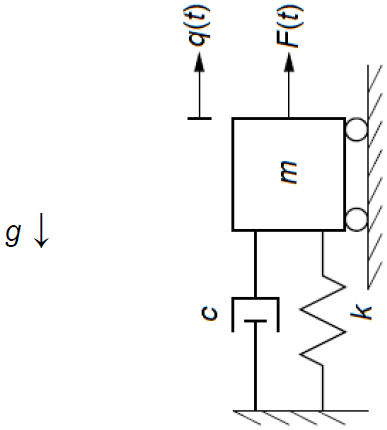
To illustrate the theory developed in Sect. 2, the equations are applied to a simple forced mass–spring–damper system. Figure 1 visualizes the system, where m is the mass, c is the damping of the dashpot, k is the stiffness of the spring, q is the displacement of the mass, F is the force applied in the direction of displacement, and g is the gravitational acceleration. The first-order system of Eq. (1) can be established by defining the states, inputs, outputs, and parameters as in Eq. (16). For illustrative purposes, the applied force is characterized as an input, and the output is arbitrarily characterized as the full motion of the mass (displacement, q; velocity, $\dot{q}$; and acceleration, $\ddot{q}$), as well as the force transmitted to the foundation, F_Transmitted. There are no constraint (algebraic) states in this system, so z and Z( ) are empty, represented by ∅, and are neglected from subsequent equations. All parameters are included in p for illustrative purposes, although gravity would not typically be a design variable.

$$\begin{array}{}\text{(16)}& \begin{array}{rl}& x=\left\{\begin{array}{c}q\\ \dot{q}\end{array}\right\},\dot{x}=\left\{\begin{array}{c}\dot{q}\\ \ddot{q}\end{array}\right\},z=\mathrm{\varnothing },u=F,\\ & y=\left\{\begin{array}{c}q\\ \dot{q}\\ \ddot{q}\\ F_{\mathrm{Transmitted}}\end{array}\right\},p=\left\{\begin{array}{c}m\\ c\\ k\\ g\end{array}\right\}\end{array}\end{array}$$

The first-order system of Eq. (1) for the simple forced mass–spring–damper system can then be written following Newton's second law, as in Eq. (17).

$$\begin{array}{}\text{(17)}& \begin{array}{l}\dot{x}=X(x,u,p)=\left[\begin{array}{ll}\mathrm{0}& \mathrm{1}\\ -\frac{k}{m}& -\frac{c}{m}\end{array}\right]x+\left\{\begin{array}{l}\mathrm{0}\\ \frac{\mathrm{1}}{m}\end{array}\right\}u+\left\{\begin{array}{l}\mathrm{0}\\ -g\end{array}\right\}\\ y=Y(x,u,p)=\left[\begin{array}{ll}\mathrm{1}& \mathrm{0}\\ \mathrm{0}& \mathrm{1}\\ -\frac{k}{m}& -\frac{c}{m}\\ k& c\end{array}\right]x+\left\{\begin{array}{l}\mathrm{0}\\ \mathrm{0}\\ \frac{\mathrm{1}}{m}\\ \mathrm{0}\end{array}\right\}u+\left\{\begin{array}{l}\mathrm{0}\\ \mathrm{0}\\ -g\\ \mathrm{0}\end{array}\right\}\end{array}\end{array}$$

The operating point in this example is taken to be the static equilibrium of the mass–spring–damper system in absence of external forcing (input), as given in Eq. (18). The simple forced mass–spring–damper system is already linear in nature, so Eq. (3) with fixed parameters can be written directly, as in Eq. (19).

$$\begin{array}{}\text{(18)}& {\displaystyle }\begin{array}{rl}& x{|}_{\mathrm{op}}=\left\{\begin{array}{l}-\frac{mg}{k}\\ \mathrm{0}\end{array}\right\},\dot{x}{|}_{\mathrm{op}}=\left\{\begin{array}{c}\mathrm{0}\\ \mathrm{0}\end{array}\right\},\\ & u{|}_{\mathrm{op}}=\mathrm{0},y{|}_{\mathrm{op}}=\left\{\begin{array}{l}-\frac{mg}{k}\\ \mathrm{0}\\ \mathrm{0}\\ -mg\end{array}\right\},p=\left\{\begin{array}{c}m\\ c\\ k\\ g\end{array}\right\}\end{array}\text{(19)}& {\displaystyle }\begin{array}{l}\mathrm{\Delta }\dot{x}=\underset{\mathbf{A}=\frac{\partial X}{\partial x}\left|{}_{\mathrm{op}}\right.}{\underbrace{\left[\begin{array}{ll}\mathrm{0}& \mathrm{1}\\ -\frac{k}{m}& -\frac{c}{m}\end{array}\right]}}\mathrm{\Delta }x+\underset{\mathbf{B}=\frac{\partial X}{\partial u}\left|{}_{\mathrm{op}}\right.}{\underbrace{\left\{\begin{array}{l}\mathrm{0}\\ \frac{\mathrm{1}}{m}\end{array}\right\}}}\mathrm{\Delta }u\\ \mathrm{\Delta }y=\underset{\mathbf{C}=\frac{\partial Y}{\partial x}\left|{}_{\mathrm{op}}\right.}{\underbrace{\left[\begin{array}{ll}\mathrm{1}& \mathrm{0}\\ \mathrm{0}& \mathrm{1}\\ -\frac{k}{m}& -\frac{c}{m}\\ k& c\end{array}\right]}}\mathrm{\Delta }x+\underset{\mathbf{D}=\frac{\partial Y}{\partial u}\left|{}_{\mathrm{op}}\right.}{\underbrace{\left\{\begin{array}{l}\mathrm{0}\\ \mathrm{0}\\ \frac{\mathrm{1}}{m}\\ \mathrm{0}\end{array}\right\}}}\mathrm{\Delta }u\end{array}\end{array}$$

Figure 1 Visualization of the forced mass–spring–damper system.

3.2 Analytical linearization with respect to parameters

Now we wish to understand the impact of small deviations in the parameters on the linear state-space model. Of course, because the linear state-space model and associated operating point have already been expressed analytically in Eqs. (18) and (19) (which is not typically the case in complex wind turbine dynamics models like OpenFAST), it is trivial to write down what the parameter-dependent variations of the linear state matrices and operating point changes should be exactly, as shown in Eqs. (20) and (21). Note that Eqs. (20) and (21) are the exact analytical expressions of the parameter-dependent linear state matrices and operating points, not derived from the theory of Sect. 2.

$$\begin{array}{}\text{(20)}& \begin{array}{rl}& \begin{array}{c}\mathbf{A}\left(\mathrm{\Delta }p\right)\\ \mathrm{exact}\end{array}=\left[\begin{array}{ll}\mathrm{0}& \mathrm{1}\\ -\frac{k+\mathrm{\Delta }k}{m+\mathrm{\Delta }m}& -\frac{c+\mathrm{\Delta }c}{m+\mathrm{\Delta }m}\end{array}\right]\\ & \begin{array}{c}\mathbf{B}\left(\mathrm{\Delta }p\right)\\ \mathrm{exact}\end{array}=\left\{\begin{array}{l}\mathrm{0}\\ \frac{\mathrm{1}}{m+\mathrm{\Delta }m}\end{array}\right\}\\ & \begin{array}{c}\mathbf{C}\left(\mathrm{\Delta }p\right)\\ \mathrm{exact}\end{array}=\left[\begin{array}{ll}\mathrm{1}& \mathrm{0}\\ \mathrm{0}& \mathrm{1}\\ -\frac{k+\mathrm{\Delta }k}{m+\mathrm{\Delta }m}& -\frac{c+\mathrm{\Delta }c}{m+\mathrm{\Delta }m}\\ k+\mathrm{\Delta }k& c+\mathrm{\Delta }c\end{array}\right]\\ & \begin{array}{c}\mathbf{D}\left(\mathrm{\Delta }p\right)\\ \mathrm{exact}\end{array}=\left\{\begin{array}{l}\mathrm{0}\\ \mathrm{0}\\ \frac{\mathrm{1}}{m+\mathrm{\Delta }m}\\ \mathrm{0}\end{array}\right\}\end{array}\end{array}$$

$$\begin{array}{}\text{(21)}& \begin{array}{rl}& \begin{array}{c}{\left.\mathrm{\Delta }x\right|}_{\mathrm{op}}\\ \mathrm{exact}\end{array}=\left\{\begin{array}{l}-\frac{(m+\mathrm{\Delta }m)(g+\mathrm{\Delta }g)}{(k+\mathrm{\Delta }k)}\\ \mathrm{0}\end{array}\right\}-\left\{\begin{array}{l}-\frac{mg}{k}\\ \mathrm{0}\end{array}\right\}\\ & =\left\{\begin{array}{l}-\frac{km\mathrm{\Delta }g+k\mathrm{\Delta }mg+k\mathrm{\Delta }m\mathrm{\Delta }g-\mathrm{\Delta }kmg}{k(k+\mathrm{\Delta }k)}\\ \mathrm{0}\end{array}\right\}\\ & \begin{array}{c}{\left.\mathrm{\Delta }y\right|}_{\mathrm{op}}\\ \mathrm{exact}\end{array}=\left\{\begin{array}{l}-\frac{(m+\mathrm{\Delta }m)(g+\mathrm{\Delta }g)}{(k+\mathrm{\Delta }k)}\\ \mathrm{0}\\ \mathrm{0}\\ -(m+\mathrm{\Delta }m)(g+\mathrm{\Delta }g)\end{array}\right\}-\left\{\begin{array}{l}-\frac{mg}{k}\\ \mathrm{0}\\ \mathrm{0}\\ -mg\end{array}\right\}\\ & =\left\{\begin{array}{l}-\frac{km\mathrm{\Delta }g+k\mathrm{\Delta }mg+k\mathrm{\Delta }m\mathrm{\Delta }g-\mathrm{\Delta }kmg}{k(k+\mathrm{\Delta }k)}\\ \mathrm{0}\\ \mathrm{0}\\ -\mathrm{\Delta }mg-m\mathrm{\Delta }g-\mathrm{\Delta }m\mathrm{\Delta }g\end{array}\right\}\end{array}\end{array}$$

3.3 Hessian-based linearization with respect to parameters

Now we wish to understand the impact of small deviations in the parameters on the linear state-space model following the theory presented in Sect. 2. In this simple example, the Hessians can be computed analytically. An example Hessian of the continuous-state functions with respect to parameters and continuous states evaluated at the operating point – written generically in Eq. (6) – is given for this simple forced mass–spring–damper example in Eq. (22). Note that in this example, N_x=2, N_z=0, N_u=1, N_y=4, and N_p=4.

$$\begin{array}{}\text{(22)}& {\left.{\displaystyle \frac{{\partial }^{\mathrm{2}}{X}_{\mathrm{1}}}{\partial p\partial x}}\right|}_{\mathrm{op}}=\left[\begin{array}{cc}\mathrm{0}& \mathrm{0}\\ \mathrm{0}& \mathrm{0}\\ \mathrm{0}& \mathrm{0}\\ \mathrm{0}& \mathrm{0}\end{array}\right],{\left.{\displaystyle \frac{{\partial }^{\mathrm{2}}{X}_{\mathrm{2}}}{\partial p\partial x}}\right|}_{\mathrm{op}}=\left[\begin{array}{ll}\frac{k}{m^{\mathrm{2}}}& \frac{c}{m^{\mathrm{2}}}\\ \mathrm{0}& -\frac{\mathrm{1}}{m}\\ -\frac{\mathrm{1}}{m}& \mathrm{0}\\ \mathrm{0}& \mathrm{0}\end{array}\right]\end{array}$$

Carrying out the remainder of the math, Eq. (23) provides the parameter-dependent variations of the linear state matrices from Eq. (9), and Eq. (24) provides the change in operating point from Eq. (11) for this simple forced mass–spring–damper example.

$$\begin{array}{}\text{(23)}& {\displaystyle }\begin{array}{rl}& \mathbf{A}\left(\mathrm{\Delta }p\right)=\left[\begin{array}{ll}\mathrm{0}& \mathrm{1}\\ \left(\frac{k\mathrm{\Delta }m}{m^{\mathrm{2}}}-\frac{(k+\mathrm{\Delta }k)}{m}\right)& \left(\frac{c\mathrm{\Delta }m}{m^{\mathrm{2}}}-\frac{(c+\mathrm{\Delta }c)}{m}\right)\end{array}\right]\\ & \mathbf{B}\left(\mathrm{\Delta }p\right)=\left\{\begin{array}{l}\mathrm{0}\\ \frac{\mathrm{1}}{m}-\frac{\mathrm{\Delta }m}{m^{\mathrm{2}}}\end{array}\right\}\\ & \mathbf{C}\left(\mathrm{\Delta }p\right)=\left[\begin{array}{ll}\mathrm{1}& \mathrm{0}\\ \mathrm{0}& \mathrm{1}\\ \left(\frac{k\mathrm{\Delta }m}{m^{\mathrm{2}}}-\frac{(k+\mathrm{\Delta }k)}{m}\right)& \left(\frac{c\mathrm{\Delta }m}{m^{\mathrm{2}}}-\frac{(c+\mathrm{\Delta }c)}{m}\right)\\ k+\mathrm{\Delta }k& c+\mathrm{\Delta }c\end{array}\right]\\ & \mathbf{D}\left(\mathrm{\Delta }p\right)=\left\{\begin{array}{l}\mathrm{0}\\ \mathrm{0}\\ \frac{\mathrm{1}}{m}-\frac{\mathrm{\Delta }m}{m^{\mathrm{2}}}\\ \mathrm{0}\end{array}\right\}\end{array}\text{(24)}& {\displaystyle }\begin{array}{rl}& {\left.\mathrm{\Delta }x\right|}_{\mathrm{op}}=\left\{\begin{array}{l}-\frac{km\mathrm{\Delta }mg-k\mathrm{\Delta }{m}^{\mathrm{2}}g+\mathrm{\Delta }km\mathrm{\Delta }mg-\mathrm{\Delta }k{m}^{\mathrm{2}}g+k{m}^{\mathrm{2}}\mathrm{\Delta }g}{k(k+\mathrm{\Delta }k)m-k^{\mathrm{2}}\mathrm{\Delta }m}\\ \mathrm{0}\end{array}\right\}\\ & {\left.\mathrm{\Delta }y\right|}_{\mathrm{op}}=\left\{\begin{array}{l}-\frac{km\mathrm{\Delta }mg-k\mathrm{\Delta }{m}^{\mathrm{2}}g+\mathrm{\Delta }km\mathrm{\Delta }mg-\mathrm{\Delta }k{m}^{\mathrm{2}}g+k{m}^{\mathrm{2}}\mathrm{\Delta }g}{k(k+\mathrm{\Delta }k)m-k^{\mathrm{2}}\mathrm{\Delta }m}\\ \mathrm{0}\\ \mathrm{0}\\ -\frac{k^{\mathrm{2}}m\mathrm{\Delta }mg+k(k+\mathrm{\Delta }k)m^{\mathrm{2}}\mathrm{\Delta }g-k(k+\mathrm{\Delta }k)\mathrm{\Delta }{m}^{\mathrm{2}}g+\mathrm{\Delta }k(k+\mathrm{\Delta }k)m\mathrm{\Delta }mg}{k(k+\mathrm{\Delta }k)m-k^{\mathrm{2}}\mathrm{\Delta }m}\end{array}\right\}\end{array}\end{array}$$

3.4 Observations

Comparing the two formulations, the exact formulation and the Hessian-based formulation – Eq. (23) with Eq. (20) and Eq. (24) with Eq. (21) – the following physical insights can be summarized.

• In the Hessian-based formulation of the parameter-dependent variations of the linear state matrices, all parameter perturbations appear linear in nature because this simple example does not have constraint states. This follows directly from item five in Sect. 2. The end result is that any parameters that are linear in nature in the underlying formulation (e.g., damping, c, and stiffness, k) are expressed exactly in the Hessian-based formulation.

• The mass, m, however, is nonlinear in the underlying formulation (showing up as $\frac{\mathrm{1}}{m}$), and so in the Hessian-based formulation of the parameter-dependent variations of the linear state matrices, the mass effect is approximated. Effectively, $\frac{\mathrm{1}}{m+\mathrm{\Delta }m}$ in the exact formulation has been approximated as $\frac{\mathrm{1}}{m}-\frac{\mathrm{\Delta }m}{m^{\mathrm{2}}}$ in the Hessian-based formulation, and equating too, we see that $m^{\mathrm{2}}\approx (m-\mathrm{\Delta }m)(m+\mathrm{\Delta }m)=m^{\mathrm{2}}-\mathrm{\Delta }{m}^{\mathrm{2}}$ only holds true when Δm²≪m², which is a second-order error. The end result is that any parameters that are nonlinear in nature in the underlying formulation are approximated to first-order accuracy in the Hessian-based formulation of the parameter-dependent variations of the linear state matrices.

• Within the operating point changes associated with the parameter variations, there are nonlinear relations of the parameter perturbations (as a result of the matrix inverse inherent in Eq. 11), which follows directly from item six in Sect. 2. However, the operating point changes are still not entirely exact in the Hessian-based formulation. It is interesting to note that the operating point changes are exact when any given parameter variation is treated in isolation (with others zeroed), e.g., $\mathrm{\Delta }q{|}_{\mathrm{op}}=-\frac{\mathrm{\Delta }mg}{k}$ and $\mathrm{\Delta }{F}_{\mathrm{Transmission}}{|}_{\mathrm{op}}=-\mathrm{\Delta }mg$ when $\mathrm{\Delta }c=\mathrm{\Delta }k=\mathrm{\Delta }g=\mathrm{0}$, likewise for other one-off parameter variations.

• When Hessians with respect to the parameters only, $\frac{{\partial }^{\mathrm{2}}}{\partial p^{\mathrm{2}}}$, are neglected, as discussed in item seven of Sect. 2, the Hessian-based operating point changes from Eq. (24) simplify a bit, as shown in Eq. (25). In Eq. (25), the operating point changes are still exact for one-off parameter variations of damping, c, and stiffness, k, and gravity, g, but the operating point changes are no longer exact when $\mathrm{\Delta }c=\mathrm{\Delta }k=\mathrm{\Delta }g=\mathrm{0}$, i.e., $\mathrm{\Delta }q{|}_{\mathrm{op}}=-\frac{m\mathrm{\Delta }mg}{k(m-\mathrm{\Delta }m)}$ and $\mathrm{\Delta }{F}_{\mathrm{Transmission}}{|}_{\mathrm{op}}=-\frac{m\mathrm{\Delta }mg}{m-\mathrm{\Delta }m}$. This demonstrates that the inclusion of the $\frac{{\partial }^{\mathrm{2}}}{\partial p^{\mathrm{2}}}$ terms in the Hessians improves the change in operating points.

  $$\begin{array}{}\text{(25)}& \begin{array}{l}\begin{array}{c}{\left.\mathrm{\Delta }x\right|}_{\mathrm{op}}\\ \mathrm{neglecting}\frac{\partial }{\partial p^{\mathrm{2}}}\end{array}=\left\{\begin{array}{l}-\frac{km\mathrm{\Delta }mg-\mathrm{\Delta }k{m}^{\mathrm{2}}g+k{m}^{\mathrm{2}}\mathrm{\Delta }g}{k(k+\mathrm{\Delta }k)m-k^{\mathrm{2}}\mathrm{\Delta }m}\\ \mathrm{0}\end{array}\right\}\\ \begin{array}{c}{\left.\mathrm{\Delta }y\right|}_{\mathrm{op}}\\ \mathrm{neglecting}\frac{\partial }{\partial p^{\mathrm{2}}}\end{array}=\left\{\begin{array}{l}-\frac{km\mathrm{\Delta }mg-\mathrm{\Delta }k{m}^{\mathrm{2}}g+k{m}^{\mathrm{2}}\mathrm{\Delta }g}{k(k+\mathrm{\Delta }k)m-k^{\mathrm{2}}\mathrm{\Delta }m}\\ \mathrm{0}\\ \mathrm{0}\\ -\frac{km\mathrm{\Delta }mg+(k+\mathrm{\Delta }k)m^{\mathrm{2}}\mathrm{\Delta }g}{(k+\mathrm{\Delta }k)m-k\mathrm{\Delta }m}\end{array}\right\}\end{array}\end{array}$$

4 Numerical implementation in WEIS

4.1 The WEIS framework

While the theoretical development presented in Sect. 2 has not been implemented in OpenFAST, we employed the direct evaluation and interpolation methods summarized in Sect. 1 within WEIS. The primary goal of WEIS is to provide a framework for the CCD of a floating wind turbine controller alongside turbine and platform geometry at multiple fidelity levels. The advantage of using WEIS for this work is that the wind turbine system is controlled by high-level design parameters (variables), wherein each variable can affect several OpenFAST inputs at once. For instance, a change of tower material mass density will change the distributed properties of the tower but also the shape functions of the tower, both of which are inputs to OpenFAST. WEIS handles such interdependencies automatically by propagating the effects of design variable changes through the entire wind turbine system. In the following subsection, we detail how we implemented the interpolation and direct evaluation methods in WEIS. Although all parameterized linear state-space matrices can be obtained following this implementation, only the parameterized state matrix, A(Δp), is used in the numerical case study (Sect. 5) and discussed below. OpenFAST was used within WEIS but not modified in any way for this work.

4.2 Design of experiments

For this article, we adapted the WEIS framework to incorporate the following workflow: call OpenFAST, retrieve the linearized state-space matrices, and store them at each evaluation call. In this study, we did not conduct the evaluations within an optimization loop but within a parametric loop, also referred to as “design of experiment” or “parameter sweep”. We extended WEIS to be able to run design of experiments where the user specifies a set of N_p design variables, $p_{n_p}$ for $n_p=\mathit{\{}\mathrm{1},\mathrm{2},\mathrm{\dots },N_p\mathit{\}}$; the interval over which the variables are to be varied, [$p_{n_p}$, min; $p_{n_p}$, max]; and the number of subdivisions of each interval (linear spacing is used). Based on these user-specified settings, WEIS evaluates for all the combinations of the design variable values. In this article, the term “parameter” is used in place of “design variables”.

4.3 Implementation of the direct evaluation method

No specific treatment is needed for the direct evaluation method. For each parameter point, $p=p{|}_{\mathrm{op}}+\mathrm{\Delta }p$ (p|_op is explicitly defined in the next section), we evaluated the linearized state matrix, A(Δp), using a call to the linearization functionality of OpenFAST. The time necessary for a direct call is on the order of minutes for land-based wind turbines and up to an hour for a complex floating offshore wind turbine. The linearization time itself only accounts for about 1 min of this total, but OpenFAST currently establishes the operating point by performing a trim solution using a time-marching loop. Because of the low frequencies of floating platforms, a significant amount of simulation time is necessary for the system to reach an equilibrium. In a separate project, we are currently working on a direct steady-state solve within OpenFAST to avoid this trim solution, which will significantly reduce the computational time needed.

Figure 2 Visualization of the interpolation method for the case with two parameter variations. (a) Nominal (operating) parameter point in blue and the bounds of the parameter interval in orange. (b) Slope (shown as the dashed–dotted line) of the state-space matrix values (shown as a continuous blue function) computed using finite differences from the bounds. (c) Interpolation step.

4.4 Implementation of the interpolation method

The implementation of the interpolation method requires two WEIS steps: a preprocessing step and a replacement of the OpenFAST call with an interpolation call. The preprocessing step proceeds as follows.

• A nominal parameter point (operating point) is defined at the center of all the parameter intervals:

  $$\begin{array}{}\text{(26)}& {\left.p_{n_p}\right|}_{\mathrm{op}}={\displaystyle \frac{p_{n_p,\max +p_{n_p},\min }}{\mathrm{2}}}\mathrm{for}{n}_p=\left\{\mathrm{1},\mathrm{2},\mathrm{\dots },N_p\right\}.\end{array}$$

• The nominal linearized state matrix is obtained using an OpenFAST call at this operating point, A.

• For each parameter, of index n_p, two OpenFAST evaluations are made to retrieve the state-space model at the bounds of the parameter interval, $\mathbf{A}\left(\mathit{\delta }{p}_{n_p}{e}_{n_p}\right)$, and $\mathbf{A}(-\mathit{\delta }{p}_{n_p}{e}_{n_p})$, wherein the parameter variation for each parameter, $\mathit{\delta }{p}_{n_p}$, is defined in Eq. (27) and $e_{n_p}$ is a unit vector the same size of p with zeros for each element except for index n_p, which equals unity:

  $$\begin{array}{}\text{(27)}& \mathit{\delta }{p}_{n_p}={\displaystyle \frac{p_{n_p,\max }-p_{n_p,\min }}{\mathrm{2}}}\mathrm{for}{n}_p=\left\{\mathrm{1},\mathrm{2},\mathrm{\dots },N_p\right\}.\end{array}$$

• The slopes, ${\left[\frac{\mathrm{d}\mathbf{A}}{\mathrm{d}p}\right]}_{n_p}$, corresponding to each parameter variation, each of which is a matrix, are then computed using a central finite difference:

  $$\begin{array}{}\text{(28)}& \begin{array}{rl}{\left[{\displaystyle \frac{\mathrm{d}\mathbf{A}}{\mathrm{d}p}}\right]}_{n_p}=& {\displaystyle \frac{\mathbf{A}\left(\mathit{\delta }{p}_{n_p}{e}_{n_p}\right)-\mathbf{A}\left(-\mathit{\delta }{p}_{n_p}{e}_{n_p}\right)}{\mathrm{2}\mathit{\delta }{p}_{n_p}}}\\ & \mathrm{for}{n}_p=\left\{\mathrm{1},\mathrm{2},\mathrm{\dots },N_p\right\}.\end{array}\end{array}$$

In total, the preprocessing steps comprise 2N_p+1 direct evaluations (calls to the OpenFAST linearization functionality). The nominal state-space model and slopes are stored for later use in the interpolation step. After the preprocessing step, the WEIS optimization loop, or design of experiment loop, proceeds as usual, but whenever a linearized state-space model is needed for a given change in operating point, Δp, instead of calling OpenFAST, an interpolation is done according to Eq. (29). The evaluation time is on the order of milliseconds, which is significantly smaller than a direct evaluation call.

$$\begin{array}{}\text{(29)}& \mathbf{A}\left(\mathrm{\Delta }p\right)=\mathbf{A}+\sum _{n_p=\mathrm{1}}^{N_p}{\left(\mathrm{\Delta }{p}_{n_p}\right)}^T{\left[{\displaystyle \frac{\mathrm{d}\mathbf{A}}{\mathrm{d}p}}\right]}_{n_p}\end{array}$$

Figure 2 illustrates the interpolation method for the case with two parameter variations (N_p=2).

5 Numerical case study using WEIS and OpenFAST

Here, we apply the numerical methods presented in Sect. 4 to the IEA 15 MW reference wind turbine (Gaertner et al., 2020), which is placed atop the University of Maine semisubmersible (Allen et al., 2020). For simplicity, the sway and roll degrees of freedom of the floater are disabled, but other relevant structural degrees of freedom are enabled. The wind turbine rotates at a constant rotor speed of 5 rpm with a blade pitch of 2.7^∘, corresponding to the operating conditions for a wind speed at hub height of 5 m s⁻¹ and a power-law exponent of 0.12. These conditions, corresponding to 10 % of rated power, were chosen to make it easier to identify the wind turbine modes (the automatic identification of modes above rated can be difficult for highly flexible rotors). We modeled the turbine using OpenFAST modules InflowWind, AeroDyn, ElastoDyn, HydroDyn, and MAP$++$. For the linearization, we modeled the aerodynamics using blade element momentum theory, with static airfoil data and frozen wake. The hydrodynamics of the platform are modeled with a hybrid combination of potential flow and a quadratic drag matrix, with the potential-flow solution in state-space form.

We chose to vary three different parameters: the tower mass density, varying between 5460 and 10140 kg m⁻³; the tower Young's modulus, varying between 1.4×10¹⁰ and 2.6×10¹⁰ N m⁻²; and the mooring line unstretched (rest) length, varying between 800 and 900 m. The variations of the tower properties correspond to ±30 % of their nominal value, whereas the rest length is varied with ±6 % because of the important nonlinearity expected for this parameter. The nominal and parameterized linear state-space matrices are obtained using both the direct and interpolation methods for all parameter combinations, using nine values per range. Based on the state matrix, we performed an eigenvalue analysis and modal identification for each set of parameters and compared the results from both methods in terms of the damped frequencies and linearized damping ratio for each full-system mode of the system. We present a subset of the results of this parametric study in the following paragraphs.

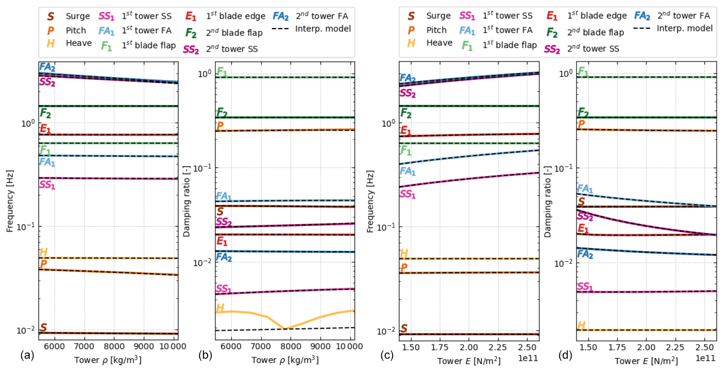
Figure 3 Variation of the system damped frequencies and damping ratios as a function of tower properties evaluated using the direct method (plain lines) and the interpolation method (dashed lines). (a, b) Variation of the tower density, ρ. (c, d) Variation of the tower Young modulus, E.

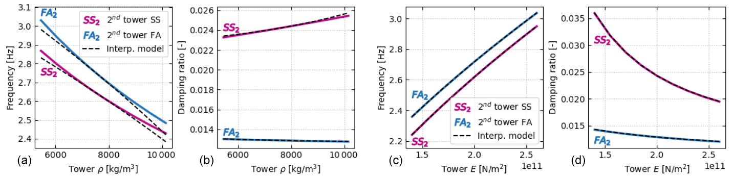
Figure 4 Variation of the second tower mode damped frequencies and damping ratios as a function of tower properties evaluated using the direct method (plain lines) and the interpolation method (dashed lines). (a, b) Variation of the tower density, ρ. (c, d) Variation of the tower Young modulus.

The results for one-dimensional variation of the tower properties are given in Fig. 3 (N_p=1). In this case, only the parameter on the abscissas is varied, and other parameters are kept at their nominal values. We used a logarithmic scale on the ordinates to better distinguish between the different modes. The following abbreviations are used in the figure for the tower modes: fore–aft (FA) bending and side–side (SS) bending. The interpolation method requires three evaluations of OpenFAST, and the direct method requires nine evaluations of OpenFAST per parameter.

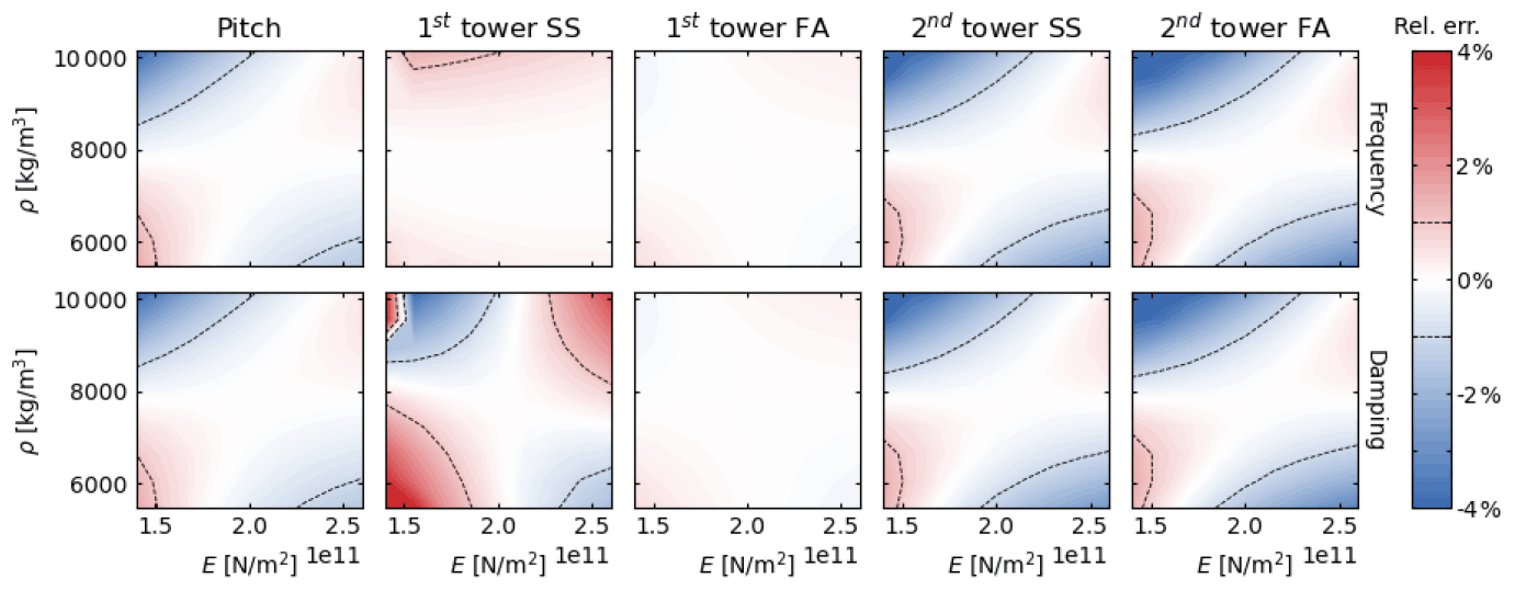
Figure 5 Relative errors in the system frequencies and damping ratios between the direct and interpolation methods as a function of tower properties (Young's modulus, E, and mass density, ρ). Top panels: relative error in damped frequencies. Bottom panels: relative error in damping ratios.

From Fig. 3, we observe that the interpolation method and the direct method are in strong agreement for all modes of the structure. With the scale provided in the figure, the curves from both methods collapse on top of each other, except for the damping of the platform-heave mode when the tower density varies. We believe this is because of the numerical sensitivity of the eigenvalue analysis and the small value of the damping of this mode. The interpolation method is only expected to return the same value as the direct method when all values of the design parameters are at the nominal value. In Fig. 3, this alignment corresponds to the middle point of the abscissas. We observe that the variations of damped frequencies and damping ratios with the tower properties are well-captured by the interpolation method, with the following expected behavior: the frequencies of the tower modes decrease with increasing density and rise with increasing stiffness. We also note that, despite the linear characteristics assumed for the state matrix in the interpolation method, the frequencies and damping ratios display nonlinear behavior after performing the eigenvalue analysis. A zoomed-in view of the variation of the second tower modes is given in Fig. 4. With this axis scale, one can observe some error between the interpolation and direct methods and that the error increases as the material density gets further away from the nominal value. No error is visible for variation of the material stiffness. This observation further exemplifies the results of Sect. 3: linearity is expected for variation of the stiffness, but variations in mass are nonlinear and hence more difficult to capture by the interpolation method.

We now present results in which the tower density and stiffness are changed together (N_p=2), using nine values for each parameter, for a total of 81 evaluations. That is, the interpolation method requires five evaluations of OpenFAST, and the direct method requires 81. The interpolated method is only expected to be exact at the center of the parametric domain, that is, at the nominal values of the tower stiffness and density. The relative error in damped frequencies and damping ratios between the interpolated and direct methods is plotted in Fig. 5 for the five modes that vary the most: the platform-pitch mode and the two first tower-bending modes in the FA and SS directions.

The results from Fig. 5 confirm that the error of the interpolation method increases as the parameters get further away from the nominal values. The error is typically smaller along lines centered on the nominal values and typically larger in the “corners”. These results are expected because the interpolation method uses slopes computed in each of the parameter directions but does not account for slopes in other (combined) directions. Overall, despite parameter variations of ±30 % of their nominal value, the error of the interpolated method remains within ±5 % for both damped frequencies and damping ratios.

In the final set of results, we present the impact of the mooring line unstretched length on the wind turbine modes as captured by both methods. Again, with N_p=1, the interpolation method requires three evaluations of OpenFAST, and the direct method requires nine evaluations of OpenFAST. As shown in Fig. 6, the mooring length mostly affects the surge mode of the semisubmersible, with some effect on the pitch mode. The interpolation method captures most of the trends, but the error in the surge mode appears more significant than what was observed for the tower study. This finding is likely the result of the strong nonlinear effect line length has on the force–displacement relationships of a catenary mooring system. Additionally, the surge mode becomes undetectable (and so is not plotted) using the state matrix obtained with the interpolation method for increased values of the mooring line unstretched length. It appears that the interpolation method fails in this situation, likely because of the numerical sensitivity of the eigenvalue analysis (i.e., the interpolation method does not provide enough precision for accurate eigensolution of all modes).

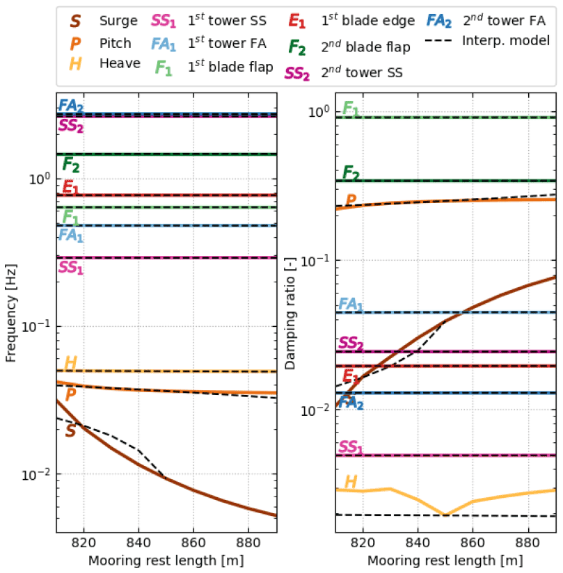
Figure 6 Variation of the system damped frequencies and damping ratios as a function of the mooring line unstretched length evaluated using the direct method (plain lines) and the interpolation method (dashed lines).

6 Conclusions

This work summarizes our efforts to better understand the impact of design parameter variations in the physical system (e.g., mass, stiffness, geometry) on the linearized system using OpenFAST. The results of this work have influenced the WEIS toolset being developed at NREL within the ATLANTIS program, with the goal of enabling CCD of the floating wind turbine structure and controller.

Theoretical developments provide some physical insights, such as the impact of design parameter variations on the operation point, the role of specific Hessians in specific state matrices and the operating point changes (including when algebraic constraint states are present) and the errors that can arise when parameters function nonlinearly within the system. These insights were further exemplified in a simple forced mass–spring–damper system example, but characteristics of the theoretical approach deterred NREL from implementing it directly within OpenFAST. Instead, we implemented a direct evaluation method and an interpolation method in the WEIS toolset, which makes use of OpenFAST, that were compared in terms of computational cost and through a numerical case study. The results from the numerical examples were encouraging for the tower study, whereby the interpolation method yielded damped frequency and damping ratio results close to the direct evaluation method despite large variation in tower density and tower Young's modulus from their nominal values. However, the interpolation method was less effective for the mooring line length study because of the strong nonlinear effect that line length has on the force–displacement relationships of a catenary mooring system. Moreover, the interpolation method failed for increased mooring rest length (with the surge mode undetectable), likely as a result of the numerical sensitivity of the eigenvalue analysis.

Improvements to the interpolation method are possible but are left as future work. For example, an N_p-linear interpolation (e.g., bilinear interpolation for N_p=2 or trilinear interpolation for N_p=3) based on values at the corners of the N_p hypercube could be used rather than using the centers of the faces of the hypercube, as is done here. Such an implementation would require ${\mathrm{2}}^{N_p}+\mathrm{1}$ evaluations of OpenFAST in the preprocessing step rather than the 2N_p+1 evaluations used here, which would improve the interpolation when multiple parameters are changed at the same time. Also, more advanced interpolations, such as N_p cubic could be postulated.

Moreover, we may reconsider implementing the calculation of Hessians directly within OpenFAST, at least for some modules and classes of parameters.