A correction method for large deflections of cantilever beams with a modal approach

Modal-based reduced-order models are preferred for modeling structures due to their computational efficiency in engineering problems. One of the important limitations of the classic modal approaches is that they are geometrically linear. This study proposes a fast correction method to account for geometric nonlinearities which stem from large deflections in cantilever beams. The method relies on pre-computed correction terms and thus adds negligibly small extra computational efforts during the time domain response analyses. The accuracy of the method is examined on a straight-beam model and International Energy Agency (IEA) 15 MW wind turbine blade model. The results show that the proposed method increases the accuracy of modal approaches significantly in secondary deflections due to nonlinearities such as axial and torsional motions for the two studied cases.

1 Introduction

Reduced-order models (ROMs) based on a modal approach are used in many structural engineering problems such as wind turbine blades (Hansen, 2015), aircraft wings (Bisplinghoff et al., 2013) and spacecraft (Marshall and Pellegrino, 2021) due to their computational efficiency and reasonable accuracy. These ROMs are based on the small-deflection assumption; in other words they use constant stiffness, mass and damping matrices which are not updated by deflections unlike nonlinear models. Hence, the accuracy of modal-based ROMs reduces as deflections increase and their errors become significant for applications with large deflections such as long and flexible wind turbine blades or aircraft wings. Moreover, the error in structural response amplifies the error in aeroelastic response and load analysis due to the coupled nature of the problem.

The large deflection effects on aeroelastic stability and loads for wind turbine blades (Kallesøe, 2011; Beardsell et al., 2016; Collier and Sanz, 2016; Riziotis et al., 2008) and aircraft wings (Cesnik et al., 2014) are now well known. Although these effects can be modeled in some aeroelastic tools by using geometric nonlinear structural solvers (Larsen and Hansen, 2019; DNV, 2016; Wang et al., 2017; Bauchau, 2009) where the stiffness matrix terms are a function of deflections or in other words nonlinear, linear modal-based ROMs are still in use even for structures with large deflections such as wind turbine blades (Branlard, 2019; Jonkman and Buhl, 2005; Branlard and Geisler, 2022) due to their speed. Therefore, it is very desirable to increase accuracy with negligible extra computational demand for such tools. This is fully aligned with the main focus of the present work.

The focus of this study is cantilever beam structures and their reduced-order models (ROMs) based on modal approaches used in coupled simulations such as aeroelasticity and load simulation of wind turbines and aircraft. A new correction method for moderately large bending deflection effects is proposed for modal-based ROMs. The method has possible minimum computational cost during the coupled analysis, since it includes only some correction terms which do not require any extra iteration during the response analysis.

Kim et al. (2009)Wang et al. (2013)Jain et al. (2017)Rutzmoser et al. (2017)Wu et al. (2018)Gözcü and Dou (2020)

Table 1 Overview of the studies with cantilever structure models. The methods, reduction bases and example cantilever structures used in the reference studies are given together with applied forces and maximum deflections in terms of span length.

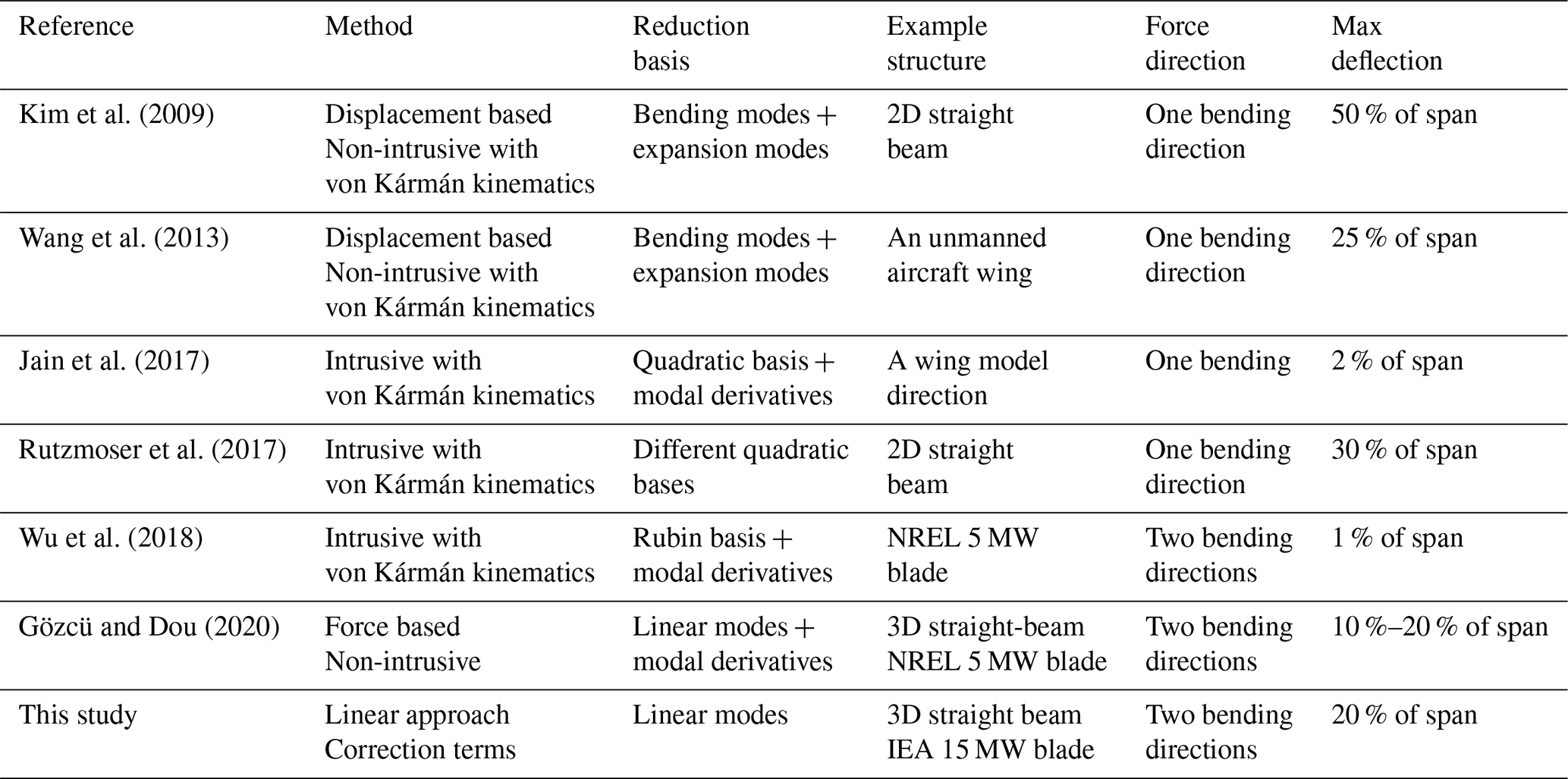
There are many studies in the literature on geometrically nonlinear ROMs, and most of them focus on clamped–clamped beams or simply supported panels. Table 1 shows some prominent works with cantilever structures from the literature together with the methods and examples used in them. The methods shown in Table 1 are either intrusive or non-intrusive. In the former, the nonlinear stiffness matrix terms in modal space are derived analytically, while the latter assumes a cubic relation between modal amplitudes and internal forces and the coefficients are determined with static analysis. As shown in the table, most of the work uses von Kármán kinematics, which are very useful for deriving the nonlinear stiffness terms as a function of displacements, and it captures the moderately large deflections accurately when plate or shell elements are used.

Intrusive and non-intrusive methods require reduction bases where the displacements are a nonlinear function of modal amplitudes. In the given studies a quadratic relation between displacements and modal amplitudes is used with modal derivatives or expansion modes which are called “dual modes” in some studies. All of these studies, except Gözcü and Dou (2020), are limited to beam models with forces applied in a single direction or forces in two bending directions with bending deflections less than 2 % of the beam span. Moreover, the methods used in existing studies require much more computational time than linear ROMs due to the iterative solutions required by nonlinear stiffness matrices. On the other hand, our proposed method uses a linear reduction basis and linear stiffness matrix for computing deflections and corrects the linear deflection results with some quadratic vectors for capturing large bending deflection effects. It may be less accurate compared to the ROMs with nonlinear stiffness terms; however it has a very similar computational speed to the existing linear ROMs and is easy to implement into existing aeroelastic tools compared to nonlinear models.

The focus of nonlinear ROMs in the literature is generally to use the same model for response and stress analysis. On the other hand, this study aims to come with a fast and accurate ROM correction method that is suitable only for response analysis and not for stress analysis. The main contributions of this paper are

• the selection of the important physics for the given applications and thus justification of particular method choice (i.e., displacement-only correction),

• a proof of method suitability using a high-fidelity model with prescribed external loads on both simple and complex geometries.

The paper is divided into the following sections. The kinematics of the cantilever beam problem relevant to this study are explained in Sect. 2, and the proposed method is explained in Sect. 3. Example cases are introduced and their results are given together with discussion in Sect. 4, and the conclusion is given in Sect. 5.

2 Relevant kinematics

This section explains the kinematics of cantilever beams and geometric nonlinear effects due to large bending deflections for symmetric beams and initially curved beams such as wind turbine blades.

Although there are many research studies about geometrically nonlinear ROMs, most of them focus on clamped–clamped beams or simply supported plates. In the clamped–clamped case, the nonlinearity arises due to the length change where a lateral deflection actually alters the length of the structure which causes an additional stiffness effect such as hardening or softening depending on the sign of length change. This effect is referred to as the membrane effect or bending–extension coupling (Touzé et al., 2021). In the case of cantilever beams, a lateral deflection due to lateral forces does not result in length change (no axial strain), so there is no bending–extension coupling for cantilever beams. However, the free end of a cantilever beam is displaced in the beam span direction to keep the length constant when it bends as shown in Fig. 1. In other words, the cantilever beams with lateral loading go through large rotations which do not result in any strain.

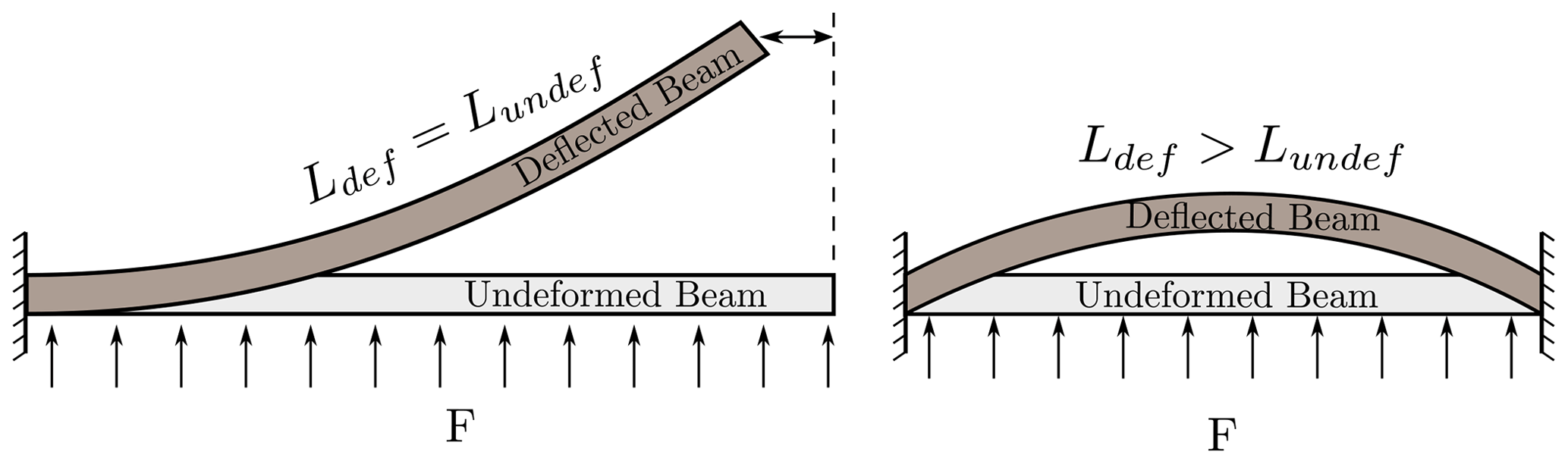
Figure 1 Displacements of a cantilever and a clamped–clamped beam under laterally distributed loads F. The deflected beam length (L_def) is equal to the undeflected length (L_undef) for the cantilever beam, resulting in zero axial strain. The clamped–clamped beam has axial strain due to elongation in beam length.

The cantilever beam in its deflected state can display a bending–torsion coupling behavior that is not seen in the undeflected state of the straight symmetric cantilever beam. Figure 2 depicts these kinematics using a straight cantilever beam. The lateral force (F_x) deflects the beam to “State-1”. Subsequently, the force perpendicular to F_x is applied to the beam which is now at “Final State”. It is observed that the beam deflects not only laterally and vertically but also in the torsion direction, even though there is no torsion load. Geometrically linear models (such as ROMs based on a modal approach) can capture bending deflections but not the torsion deflection for this problem, since their stiffness matrices are not updated by new states or deflections.

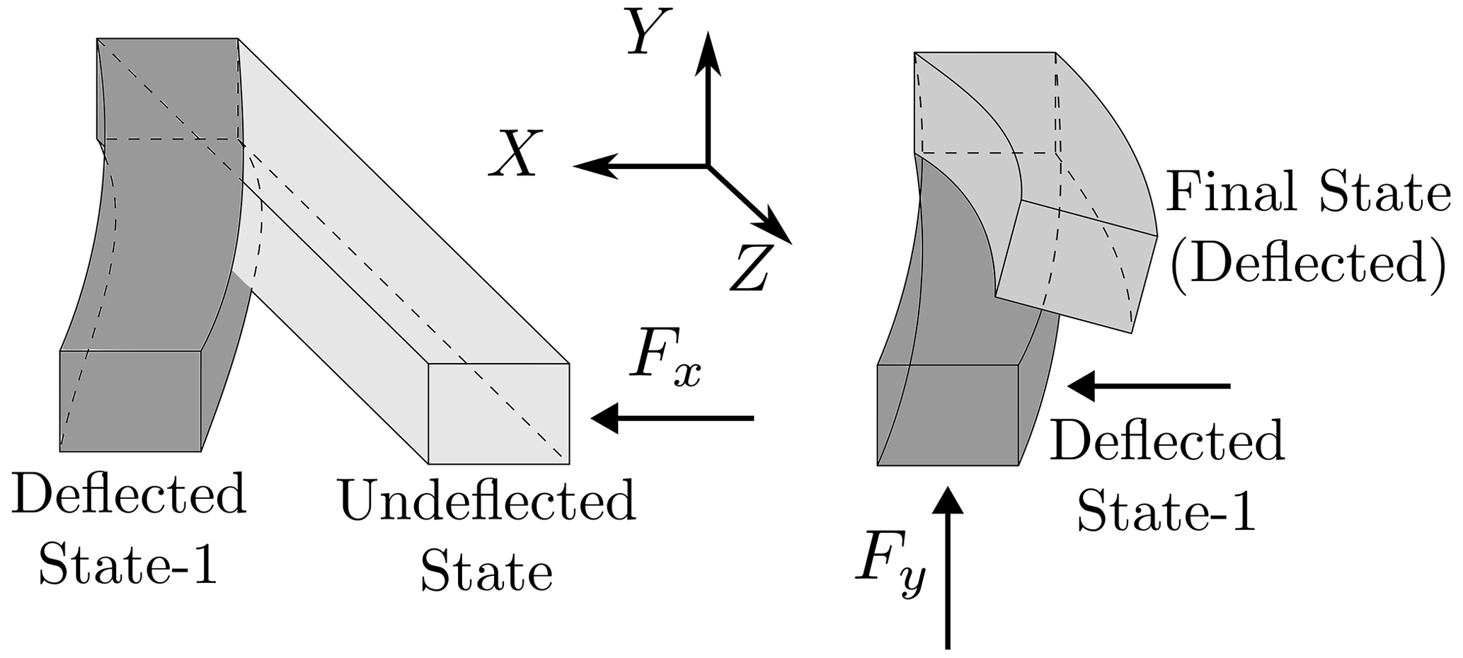
Figure 2 Illustration of beam deflections in lateral directions and the resulting torsion motion due to the bending–torsion coupling at the deflected state. The lateral (x, y) and axial (z) directions are given in beam root coordinates.

These kinematics become even more prominent for applications such as wind turbine blades, which are initially curved structures due to prebend. They already have bending–torsion couplings at their undeflected states, but the lateral deflections change the magnitude as well as the direction of this coupling. Figure 3 shows the torsion deflection due to the combination of flapwise and edgewise deflections of a wind turbine blade with prebend at its undeflected position. The edgewise and torsion motions are already coupled for a blade with prebend as shown in the figure. However this coupling first reduces and then changes sign with flapwise bending deflections. As the blade goes through sinusoidal edgewise bending deflections due to gravity and rotation, the torsion induced by edgewise–torsion coupling also alters blade loads and aeroelastic stability (Kallesøe, 2011). These coupling effects become significant for very flexible wind turbine blades. In the case geometrically linear models like classical ROMs based on modal reduction are used, the change in torsion–edgewise coupling cannot be captured correctly for large blade deflections.

Figure 3 Illustration of wind turbine deflections in flapwise (y) and edgewise (x) directions and the resulting torsion motion due to the bending–torsion coupling at the deflected state. The lateral (x, y) and axial (z) directions are given in blade root coordinates. The effective blade length is the projected length onto the root coordinate system in the axial direction. The edgewise–torsion coupling at the initial blade position has an opposite direction in comparison to the edgewise–torsion coupling at the deflected blade position.

Here, the kinematics of a cantilever beam due to bending deflections are explained and kinematics due to axial–bending coupling are left without mentioning since the proposed method is developed only for secondary effects due to large bending deflections of cantilever beams. Hence, the method cannot capture stiffening effects with centrifugal force (Wallrapp and Schwertassek, 1991; Branlard and Geisler, 2022) which comes from bending–extension coupling. However, centrifugal stiffening is already corrected for linear models in existing tools such as Flex (Branlard, 2019) and FAST (Jonkman and Buhl, 2005). In this study, mode shapes at an undeformed state without centrifugal stiffening effects are use, since the mentioned existing tools compute blade mode shapes at undeflected states. However, the method is not limited with undeflected state modal analysis, and it can also work with mode shapes computed at any deflected state.

3 Method

The nonlinear geometric effects of a cantilever beam can be captured by nonlinear ROMs using different methods (intrusive or non-intrusive; see Table 1) and a reduction basis where linear modes are used together with quadratic vectors such as expansion modes (Hollkamp and Gordon, 2008) or modal derivatives (Idelsohn and Cardona, 1985). It is observed that effects of nonlinear stiffness terms such as stiffening are not significant in bending directions for moderately large deflections of a cantilever beam. On the other hand, the geometric nonlinear effects explained in Sect. 2 are still apparent for cantilever beams.

These kinematics together with other nonlinear effects such as centrifugal stiffening are captured very accurately by geometrically nonlinear models which come with much higher computational cost compared to linear ROMs. Our method uses linear ROMs which use linear mode shapes, stiffness, mass and damping matrices for response calculation, and quadratic vectors are added to the linear response results to capture large bending deflection effects. In the studies where intrusive methods are used, modal derivatives are generally preferred as quadratic vectors for deriving nonlinear stiffness terms in modal space. For non-intrusive methods, the terms for the cubic relation between modal amplitudes and reduced stiffness terms are obtained from some static solutions and the reduction basis includes generally expansion modes. In this study, both modal derivatives and expansion modes are investigated as correction terms for large bending effects. The formulation and calculation process of these vectors are explained below.

3.1 Modal derivatives

The modal derivatives (MDs) are quadratic vectors which include secondary effects that occur due to large deflections (geometric nonlinearities) (Idelsohn and Cardona, 1985; Wu and Tiso, 2014). The quadratic relation needs to be written between physical displacements (u) and modal amplitudes (q) for defining modal derivatives. So, they can be thought of as a second derivative of physical displacements (u) with respect to modal amplitudes (q) when the displacements are represented as a function of modal amplitudes. When Taylor series expansion of the displacements around an equilibrium state (u₀=u(q₀)) is written, the first term (u(q₀)) is the equilibrium state, the first derivative represents the linear mode shapes and the second derivative term includes the modal derivatives as shown in Eq. (1).

$$\begin{array}{}\text{(1)}& \begin{array}{rl}\mathit{u}\left(\mathit{q}\right)& \approx \mathit{u}\left({\mathit{q}}_{\mathrm{0}}\right)+{\left.{\displaystyle \frac{\partial \mathit{u}}{\partial \mathit{q}}}\right|}_{{\mathit{q}}_{\mathrm{0}}}\cdot \left(\mathit{q}-{\mathit{q}}_{\mathrm{0}}\right)+{\displaystyle \frac{\mathrm{1}}{\mathrm{2}}}\left({\left.{\displaystyle \frac{{\partial }^{\mathrm{2}}\mathit{u}}{\partial \mathit{q}\partial \mathit{q}}}\right|}_{{\mathit{q}}_{\mathrm{0}}}\cdot \left(\mathit{q}-{\mathit{q}}_{\mathrm{0}}\right)\right)\\ & \cdot \left(\mathit{q}-{\mathit{q}}_{\mathrm{0}}\right)+\mathcal{O}\left({∥\mathit{q}∥}^{\mathrm{3}}\right)=\mathit{u}\left({\mathit{q}}_{\mathrm{0}}\right)+\mathbf{\Phi }\cdot \mathit{q}+{\displaystyle \frac{\mathrm{1}}{\mathrm{2}}}\left({\displaystyle \frac{\partial \mathbf{\Phi }}{\partial \mathit{q}}}\cdot \mathit{q}\right)\\ & \cdot \mathit{q}+\mathcal{O}\left(\Vert \mathit{q}{\Vert }^{\mathrm{3}}\right)\end{array}\end{array}$$

In this study, the equilibrium state is taken as the initial state where u₀=0 (undeflected state) and Eq. (1) can be written in terms of mode shapes and their derivatives at the initial state as

$$\begin{array}{}\text{(2)}& \mathit{u}\left(\mathit{q}\right)\approx \mathbf{\Phi }\cdot \mathit{q}+{\displaystyle \frac{\mathrm{1}}{\mathrm{2}}}\left({\displaystyle \frac{\partial \mathbf{\Phi }}{\partial \mathit{q}}}\cdot \mathit{q}\right)\cdot \mathit{q}+\mathcal{O}\left(\Vert \mathit{q}{\Vert }^{\mathrm{3}}\right),\end{array}$$

where Φ is linear mode shapes, u is the displacement vector and q is the modal amplitude vector. The displacement vector is a function of time (t) and position (x), whereas mode shapes are only a function of position (x) and modal amplitudes are only function of time (t). So, they can be written as u(t,x), q(t) and Φ(x); however their time and position relations are not included in the equations for simplicity. The linear mode shapes (Φ) and corresponding natural frequencies (ω) can be found by the generalized eigenvalue solution,

$$\begin{array}{}\text{(3)}& \left(\mathbf{K}-{\mathit{\omega }}_i^{\mathrm{2}}\mathbf{M}\right){\mathit{\varphi }}_i=\mathbf{0},\end{array}$$

where K and M are the tangent stiffness and mass matrices and ω_i and ϕ_i are the ith eigenvalue and corresponding eigenvector (mode shape vector). The tangent stiffness is the Jacobian of the internal force with respect to the displacement. It is a generalization of the linear stiffness matrix in the nonlinear case. Here the tangent stiffness and mass matrices are computed at the initial state (u₀=0) for the purpose of solving eigenvalue problems. As seen in the later derivation in this section, the tangent stiffness at the deflected state is also required to compute the modal derivatives. The modal derivatives are calculated by taking the derivative of the eigenvalue problem shown in Eq. (3) with respect to modal amplitude q_j.

$$\begin{array}{}\text{(4)}& \begin{array}{rl}{\displaystyle \frac{\partial }{\partial q_j}}\left(\left(\mathbf{K}-{\mathit{\omega }}_i^{\mathrm{2}}\mathbf{M}\right){\mathit{\varphi }}_i\right)& =\left({\displaystyle \frac{\partial \mathbf{K}}{\partial q_j}}-{\displaystyle \frac{\partial {\mathit{\omega }}_i^{\mathrm{2}}}{\partial q_j}}\mathbf{M}-{\mathit{\omega }}_i^{\mathrm{2}}{\displaystyle \frac{\partial \mathbf{M}}{\partial q_j}}\right){\mathit{\varphi }}_i\\ & +\left(\mathbf{K}-{\mathit{\omega }}_i^{\mathrm{2}}\mathbf{M}\right){\displaystyle \frac{\partial {\mathit{\varphi }}_i}{\partial q_j}}=\mathrm{0}\end{array}\end{array}$$

To determine the derivative of ϕ_i and ω_i with respect to the jth modal amplitude q_j, another equation is needed. This equation can be chosen as Eq. (5), where ϕ_i is the mass-normalized mode shape vector.

$$\begin{array}{}\text{(5)}& \begin{array}{rl}{\displaystyle \frac{\partial }{\partial q_j}}& \left({\mathit{\varphi }}_i^T\mathbf{M}{\mathit{\varphi }}_i\right)=\mathrm{2}{\mathit{\varphi }}_i^T{\mathbf{M}}^T{\displaystyle \frac{\partial {\mathit{\varphi }}_i}{\partial q_j}}+{\mathit{\varphi }}_i^T{\displaystyle \frac{\partial \mathbf{M}}{\partial q_j}}{\mathit{\varphi }}_i=\mathrm{0},\\ & \mathrm{where}{\mathit{\varphi }}_i^T\mathbf{M}{\mathit{\varphi }}_i=\mathrm{1}.\end{array}\end{array}$$

When Eqs. (4) and (5) are combined, the modal derivative of the ith mode shape vector ϕ_i and natural frequency ω_i with respect to the jth modal amplitude can be determined by

$$\begin{array}{}\text{(6)}& \left[\begin{array}{cc}\left(\mathbf{K}-{\mathit{\omega }}_i^{\mathrm{2}}\mathbf{M}\right)& -\mathbf{M}{\mathit{\varphi }}_i\\ -{\left(\mathbf{M}{\mathit{\varphi }}_i\right)}^T& \mathrm{0}\end{array}\right]\left[\begin{array}{c}\frac{\partial {\mathit{\varphi }}_i}{\partial q_j}\\ \frac{\partial {\mathit{\omega }}_i^{\mathrm{2}}}{\partial q_j}\end{array}\right]=\left[\begin{array}{c}-\frac{\partial \mathbf{K}}{\partial q_j}{\mathit{\varphi }}_i+{\mathit{\omega }}_i^{\mathrm{2}}\frac{\partial \mathbf{M}}{\partial q_j}{\mathit{\varphi }}_i\\ \frac{\mathrm{1}}{\mathrm{2}}{\mathit{\varphi }}_i^T\frac{\partial \mathbf{M}}{\partial q_j}{\mathit{\varphi }}_i\end{array}\right].\end{array}$$

Equation (6) contains all the terms that are required to compute the modal derivatives. The derivation of modal derivatives is similar to the derivation of the sensitivity of eigenmodes and eigenfrequencies with respect to a design variable in structural optimization.

For computation of modal derivatives, the terms related to inertia effects (i.e., mass matrix and its derivatives) are generally ignored, since their contribution to the modal derivatives is very limited (Rutzmoser et al., 2017). The derivative of the eigenvalue can also be assumed to be zero due to the fact the eigenfrequencies of the slender cantilever beams are not sensitive to the vibration amplitude. These assumptions lead to static modal derivatives which are symmetric, whereas modal derivatives computed from Eq. (6) are not necessarily symmetric.

$$\begin{array}{}\text{(7)}& {\displaystyle \frac{\partial \mathit{\varphi }i}{\partial q_j}}=-{\mathbf{K}}^{-\mathrm{1}}{\displaystyle \frac{\partial \mathbf{K}}{\partial q_j}}{\mathit{\varphi }}_i\end{array}$$

For conciseness, the static modal derivatives are simply called modal derivatives (MDs) hereafter. In Eq. (7), the derivative of the stiffness matrix with respect to the jth modal amplitudes, i.e., $\frac{\partial \mathbf{K}}{\partial q_j}$, is needed to compute the modal derivatives. In this study, the derivative of the stiffness matrix (K) with respect to the jth modal amplitudes (q_j) is computed by central finite differences as

$$\begin{array}{}\text{(8)}& {\displaystyle \frac{\partial \mathbf{K}}{\partial q_j}}={\displaystyle \frac{\mathbf{K}\left({\mathit{\varphi }}_j{\mathit{\delta }}_j\right)-\mathbf{K}\left(-{\mathit{\varphi }}_j{\mathit{\delta }}_j\right)}{\mathrm{2}{\mathit{\delta }}_j}},\end{array}$$

where K(ϕ_jδ_j) is the tangent stiffness matrix when the system displacements equal ϕ_jδ_j. The tangent stiffness matrix at the deflected state of the structure by a given amplitude of δ_j is computed with a geometrically nonlinear beam solver based on the co-rotational formulation (https://doi.org/10.5281/zenodo.7533686) in Krenk (2005). The calculation of $\frac{\partial \mathbf{K}}{\partial q_j}$ from Eq. (8) is the only step where a geometrically nonlinear solver is required. When the stiffness matrix derivatives are ready, the computation of Eq. (7) is straightforward, since the rest of the equation consists of the stiffness matrix and linear eigenvectors at the undeflected state. The tangent stiffness matrix at the undeflected state is actually the linear stiffness matrix which is used in existing modal approaches. There are M_MD number of modal derivatives which are computed for M number of linear mode shapes. The relation between M and M_MD can be written as

$$\begin{array}{}\text{(9)}& M_{\mathrm{MD}}={\displaystyle \frac{M\times (M+\mathrm{1})}{\mathrm{2}}}.\end{array}$$

Figures 4 and 5 are used to give visual understanding of the modal derivatives. Figure 4 shows bending of a straight beam with an airfoil cross-section in one direction and its representation by a linear bending mode and its modal derivative by itself. The linear bending mode shape does not have any displacement in the axial (spanwise) direction, so the total (curved) length of the beam increases. The modal derivative vector of the bending mode shape with respect to its modal amplitude includes the axial displacement effect. When the linear bending mode and its modal derivative are summed, the axial displacement and bending effects are captured together.

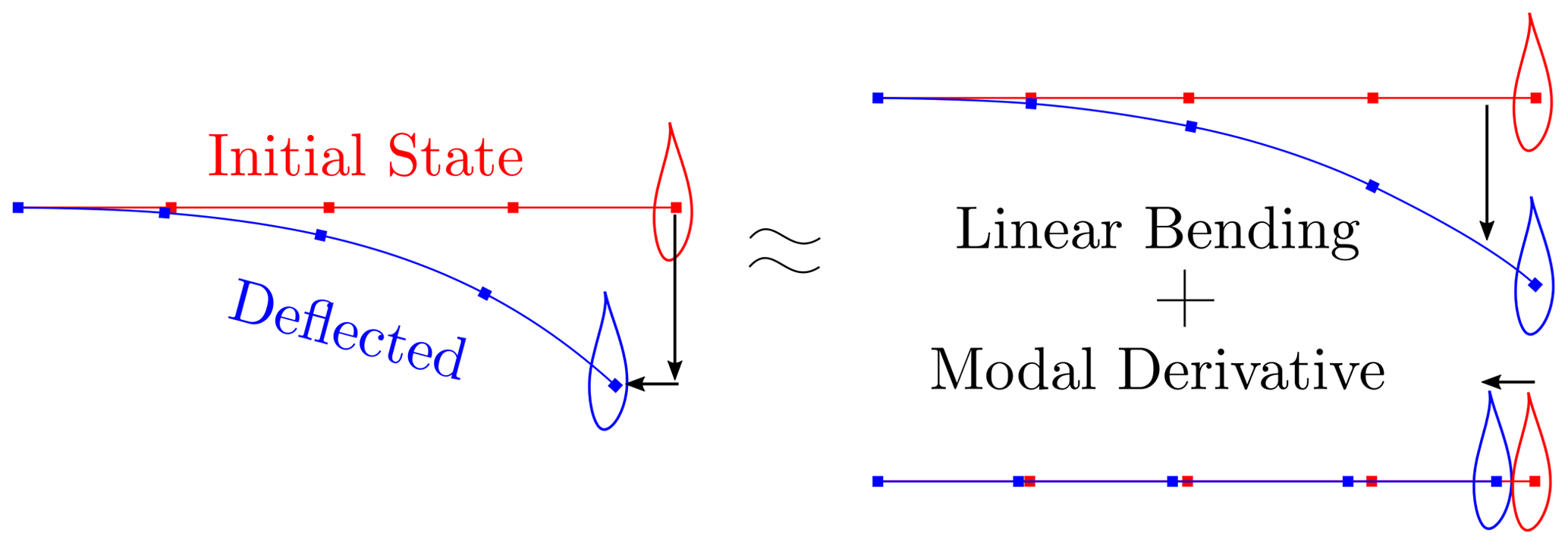
Figure 4 Bending deflection of a straight beam in the first mode shape and its representation by linear mode shape and its modal derivatives.

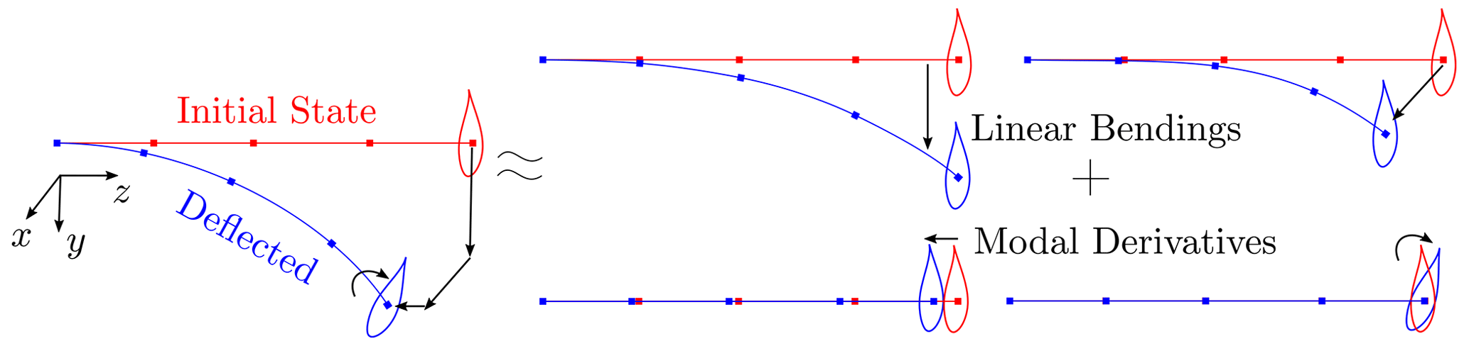
Figure 5 Bending deflections of a straight beam in lateral (x and y) directions and the representation of the deflections by linear mode shapes and their modal derivatives.

Figure 5 shows the modal derivatives that are similar to that in Fig. 4 except that the deflections occur in two bending directions at the same time. Hence, together with the axial displacements, there is also a torsion effect due to the couplings at the deflected state. The linear modal approach is only capable of capturing the bending deflections in two lateral (x and y) directions. The axial displacements are captured by the modal derivatives of each bending mode shape with respect to its own modal amplitudes in Fig. 5, whereas the torsion effects are included in the cross-modal derivative vectors which are the derivatives of one bending mode shape with respect to the modal amplitudes of another bending mode in the other direction.

3.2 Expansion modes

Expansion modes are similar to modal derivatives, but they are computed by a non-intrusive approach (Hollkamp and Gordon, 2008). The expansion modes also contain the secondary effects such as the axial and torsion motions caused by the bending motions. These vectors are computed from the difference between the deflections computed by linear ROMs and the nonlinear deflections. The difference is written as a function of the selected order of modal amplitudes, and a quadratic (second-order) relation is used in this study. Nonlinear deflections for static cases are computed in a geometrically nonlinear solver. In the expansion mode approach, the physical displacements are represented as

$$\begin{array}{}\text{(10)}& {\displaystyle }\mathit{u}(t,x)\approx \mathbf{\Phi }\left(x\right)\mathit{q}\left(t\right)+{\mathbf{\Phi }}_{\mathrm{EM}}\left(x\right){\mathit{q}}_{\mathrm{EM}}\left(t\right),\end{array}$$

where Φ and Φ_EM are the matrices whose columns are the linear modes and the expansion modes, x is position, and t is time. The expansion mode amplitudes q_EM are quadratic functions of the bending modes and can be written in terms of the M linear mode amplitudes as

$$\begin{array}{}\text{(11)}& \begin{array}{rl}& {\mathit{q}}_{\mathrm{EM}}=\\ & {\left[\begin{array}{ccccccc}{q}_{\mathrm{1}}^{\mathrm{2}}& q_{\mathrm{1}}{q}_{\mathrm{2}}\mathrm{\dots }& q_{\mathrm{1}}{q}_{\mathrm{M}}& q_{\mathrm{2}}^{\mathrm{2}}& q_{\mathrm{2}}{q}_{\mathrm{3}}\mathrm{\dots }& q_{(\mathrm{M}-\mathrm{1})}{q}_{\mathrm{M}}& q_{\mathrm{M}}^{\mathrm{2}}\end{array}\right]}^T,\end{array}\end{array}$$

where q_i is the ith linear mode amplitudes. The relation between the number of linear modes (M) and the number of corresponding expansion modes (M_EM) is

$$\begin{array}{}\text{(12)}& M_{\mathrm{EM}}={\displaystyle \frac{M\times (M+\mathrm{1})}{\mathrm{2}}}.\end{array}$$

So, there are the same number of modal derivatives and expansion modes for the same number of linear modes, since both of these vectors represent the quadratic relation between deflections and modal amplitudes.

While the above Eq. (10) defines the expansion modes, the procedure to compute the expansion modes is given below.

First, a set of static analyses are performed. The applied forces are chosen as a combination of two linear mode shapes (Φ), which can be written as

$$\begin{array}{}\text{(13)}& \mathit{f}=\mathbf{K}\left({\mathit{\lambda }}_i{\mathbf{\Phi }}_i+{\mathit{\lambda }}_j{\mathbf{\Phi }}_j\right),\end{array}$$

where λ_i and λ_j are the prescribed scaling factors for the ith and jth linear mode shape. The nonlinear displacements (u) are computed with a geometrically nonlinear solver for the loads f.

Second, the amplitudes of the linear modes, i.e., q, are computed from the applied loads as

$$\begin{array}{}\text{(14)}& \begin{array}{rl}& {\mathbf{\Phi }}^T\mathbf{K}\mathbf{\Phi }\mathit{q}={\mathbf{\Phi }}^T\mathit{f}={\mathbf{K}}_{\mathrm{r}}\mathit{q}={\mathit{f}}_{\mathrm{r}}\\ & \mathit{q}={\mathbf{K}}_{\mathrm{r}}^{-\mathrm{1}}{\mathit{f}}_{\mathrm{r}},\end{array}\end{array}$$

where K and K_r are the full and reduced stiffness matrices and f and f_r are the full and reduced force vectors. When the applied forces (f) are known, q can be computed.

Once we have the linear modal amplitudes (q), the corresponding expansion modal amplitudes (q_EM) can be computed by using Eq. (11).

Then, the nonlinear displacements, the amplitudes of the linear modes and the amplitudes of the expansion modes can be collected into three matrices: $\mathbf{U}\in {\mathbb{R}}^{N\times N_k}$, $\mathbf{Q}\in {\mathbb{R}}^{M\times N_k}$ and ${\mathbf{Q}}_{\mathrm{EM}}\in {\mathbb{R}}^{M_{\mathrm{EM}}\times N_k}$. Here each column of the matrices corresponds to a static load case. All load case results can be written in matrix form as

$$\begin{array}{}\text{(15)}& \mathbf{U}\approx \mathbf{\Phi }\mathbf{Q}+{\mathbf{\Phi }}_{\mathrm{EM}}{\mathbf{Q}}_{\mathrm{EM}}.\end{array}$$

Equation (15) is similar to Eq. (10) except that Eq. (15) is in matrix form where the nonlinear displacements U, the linear modes Φ and the amplitudes of the linear modes Q are known from the above steps. The only unknown in Eq. (15) is the expansion modes Φ_EM.

Finally, the expansion modes can be determined by using the least-squares method:

$$\begin{array}{}\text{(16)}& {\mathbf{\Phi }}_{\mathrm{EM}}{\mathbf{Q}}_{\mathrm{EM}}=\mathbf{U}-\mathbf{\Phi }\mathbf{Q}⟶\underset{{\mathbf{\Phi }}_{\mathrm{EM}}\in {\mathbb{R}}^{N\times M_{\mathrm{EM}}}}{\mathrm{minimize}}\left|\mathbf{U}-\mathbf{\Phi }\mathbf{Q}-{\mathbf{\Phi }}_{\mathrm{EM}}{\mathbf{Q}}_{\mathrm{EM}}\right.∥,\end{array}$$

where $\Vert \Vert$ denotes the Euclidean or L² norm of the vector and it is solved for modal expansion matrix Φ_EM.

It is noted that the expansion modes are very similar to the modal derivatives. They are identical except the numeric differences if the sets of the ith and jth are symmetric and the force amplitudes λ_i and λ_j are small enough. The computational cost of the expansion modes is more expensive than the modal derivatives, since their calculation requires solving more static problems than the calculation of the modal derivatives. The difference in the computational cost is small when the number of linear modes (M) is small. However, this difference becomes significant when the number of the linear modes is large.

Further, it is noted that one can extend Eq. (11) to include higher-order expansion modes corresponding to higher-order polynomial terms of the amplitudes of the linear modes, for example, the expansion modes for the cubic and quadratic terms of the linear modal amplitudes.

3.3 Numerical implementation

As mentioned before, the modal derivatives or the expansion modes are not included in the reduction space. Consequently, only the linear mass, stiffness and damping matrices are used in the dynamic response analysis. This is not the case for other studies in the literature (see Table 1), which have used the nonlinear stiffness terms in the modal space.

Algorithm 1 shows the procedure to obtain a structural response with correction vectors for pure structural response analysis where the forces are functions of time and for coupled response analysis where the forces are functions of both time and displacements. In this study, modal derivative and expansion mode vectors are used as correction vectors.

Algorithm 1 Response calculation with quadratic correction vectors.

• Model generation step (time independent and done once)

  1. Generate the linear ROM from the finite element model:

     1. Compute the linear modes (ϕ_i) from $\left(\mathbf{K}-{\mathit{\omega }}_i^{\mathrm{2}}\mathbf{M}\right){\mathit{\varphi }}_i=\mathbf{0}$

     2. Compute the reduced-order stiffness K_r, mass M_r and damping C_r matrices by Galerkin projection:
        K_r=Φ^TKΦ, M_r=Φ^TMΦ, C_r=Φ^TCΦ

  2. Compute the correction vectors:
     For the modal derivatives see Sect. 3.1
     For the expansion modes see Sect. 3.2

• Pure structural response analysis (forces are functions of time)

  1. Compute the modal amplitudes for the linear ROM by solving the equation of motion:
     ${\mathbf{M}}_{\mathrm{r}}\ddot{\mathit{q}}\left(t\right)+{\mathbf{C}}_{\mathrm{r}}\dot{\mathit{q}}\left(t\right)+{\mathbf{K}}_{\mathrm{r}}\mathit{q}\left(t\right)={\mathbf{\Phi }}^T\mathit{f}\left(t\right)={\mathit{f}}_{\mathrm{r}}\left(t\right)$

  2. Compute the displacements by using the linear modes, the correction vectors and the linear modal amplitudes:
     With MDs : $\mathit{u}(x,t)=\mathbf{\Phi }\left(x\right)\cdot \mathit{q}\left(t\right)+\frac{\mathrm{1}}{\mathrm{2}}\left(\frac{\partial \mathbf{\Phi }}{\partial \mathit{q}}\cdot \mathit{q}\left(t\right)\right)\cdot \mathit{q}\left(t\right)$
     With EMs: $\mathit{u}(x,t)=\mathbf{\Phi }\left(x\right)\mathit{q}\left(t\right)+{\mathbf{\Phi }}_{\mathrm{E}}\left(x\right){\mathit{q}}_{\mathrm{E}}\left(q\right)$
     The calculation of displacements (u(x,t)) does not have to be done at each time step and can be performed as a post-process after the time simulations.

• Coupled response analysis (forces are functions of time and displacements)

  1. Compute modal amplitudes for linear ROM by solving equation of motion:
     ${\mathbf{M}}_{\mathrm{r}}\ddot{\mathit{q}}\left(t\right)+{\mathbf{C}}_{\mathrm{r}}\dot{\mathit{q}}\left(t\right)+{\mathbf{K}}_{\mathrm{r}}\mathit{q}\left(t\right)={\mathbf{\Phi }}^T\mathit{f}(t,\mathit{u})={\mathit{f}}_{\mathrm{r}}(t,\mathit{u})$

  2. Compute displacements by using linear modes, correction vectors, and the linear modal amplitudes:
     With MDs: $\mathit{u}(x,t)=\mathbf{\Phi }\left(x\right)\cdot \mathit{q}\left(t\right)+\frac{\mathrm{1}}{\mathrm{2}}\left(\frac{\partial \mathbf{\Phi }}{\partial \mathit{q}}\cdot \mathit{q}\left(t\right)\right)\cdot \mathit{q}\left(t\right)$
     With EMs: $\mathit{u}(x,t)=\mathbf{\Phi }\left(x\right)\mathit{q}\left(t\right)+{\mathbf{\Phi }}_{\mathrm{E}}\left(x\right){\mathit{q}}_{\mathrm{E}}\left(q\right)$

  3. Update the loads (f(t,u)) and apply the loads

4 Results and discussion

The proposed method is demonstrated in the case studies of a straight cantilever beam and the blade of the International Energy Agency (IEA) 15 MW reference wind turbine under static and dynamic loads. The displacement results are given to evaluate the effectiveness of the correction methods based on the modal derivatives and expansion modes to capture the large bending deflection effects. The reduced-order model results are compared with HAWC2 results for both static and dynamic cases. HAWC2 (Larsen and Hansen, 2019) is an aero-servo-hydro-elastic load analysis tool for wind turbines and has been developed by DTU Wind and Energy Systems. It uses multibody formulation with Timoshenko beam and can capture geometric nonlinearities (Pavese et al., 2016). In HAWC2, the z axis is along the axial direction, whereas the x and y directions are lateral directions (see Fig. 3 for the HAWC2 coordinate system).

4.1 Straight beam

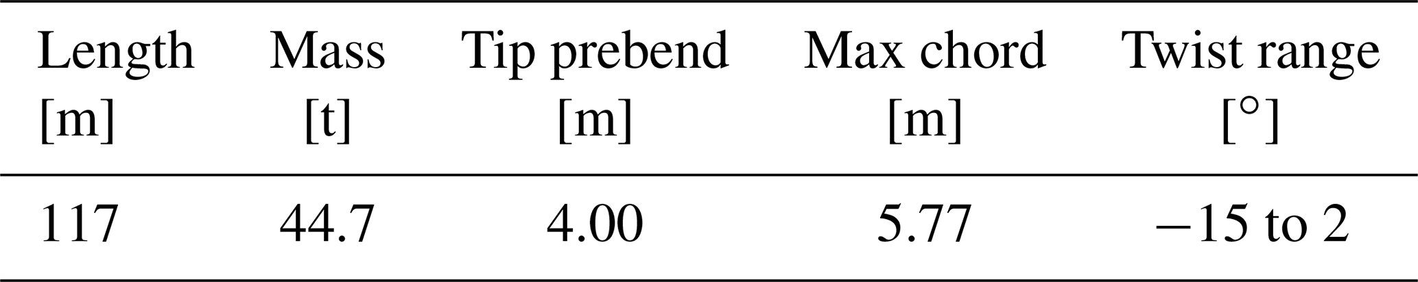
A cantilever straight-beam model is used for static and dynamic load cases. Table 2 shows the general properties of the beam, whose cross-section properties are constant along the beam length and shear coefficients are very high compared to the bending stiffness values, so it behaves like an Euler–Bernoulli beam.

Table 2 Straight-beam geometry and cross-section stiffness properties. Beam is clamped from its root.

Figure 6 shows x, y, z displacement and torsion motion components of the first two mode-shape vectors of the beam. Since the beam is straight and has no material coupling, both bending mode shapes have only one lateral-direction displacement without any axial or torsion component. The first mode shape is in the x direction, and the second one is in the y direction.

Figure 6 x, y, z and torsion components of first two mode shapes of straight beam. Beam span is along the z axis.

Figure 7 shows modal derivative (MD) and expansion mode (EM) vectors for first two mode shapes. The results are very similar for MD and EM vectors. These vectors show the sensitivity of a mode shape with respect to a modal amplitude. The vector names are given so that the first number represents the mode number for the linear mode-shape vector whose sensitivity is computed with respect to the modal amplitude of the mode number, which is given as the second number in the vector names. Hence, MD-1-1, MD-2-2, EM-1-1 and EM-2-2 show the sensitivity of a mode shape with respect to its own modal amplitude, whereas MD-1-2 and EM-1-2 illustrate the sensitivity of a mode shape with respect to another mode's modal amplitude. Since MD-2-1 and MD-1-2 are the same for static modal derivatives, only MD-1-2 results are shown here. This symmetry case is also valid for expansion modes (EMs), since they are also computed for static cases. MD-i-i and EM-i-i vectors have only axial displacements since their mode shapes are only in one lateral direction. On the other hand, MD-i-j and EM-i-j have only torsion motions, which represent the coupling between two lateral directions.

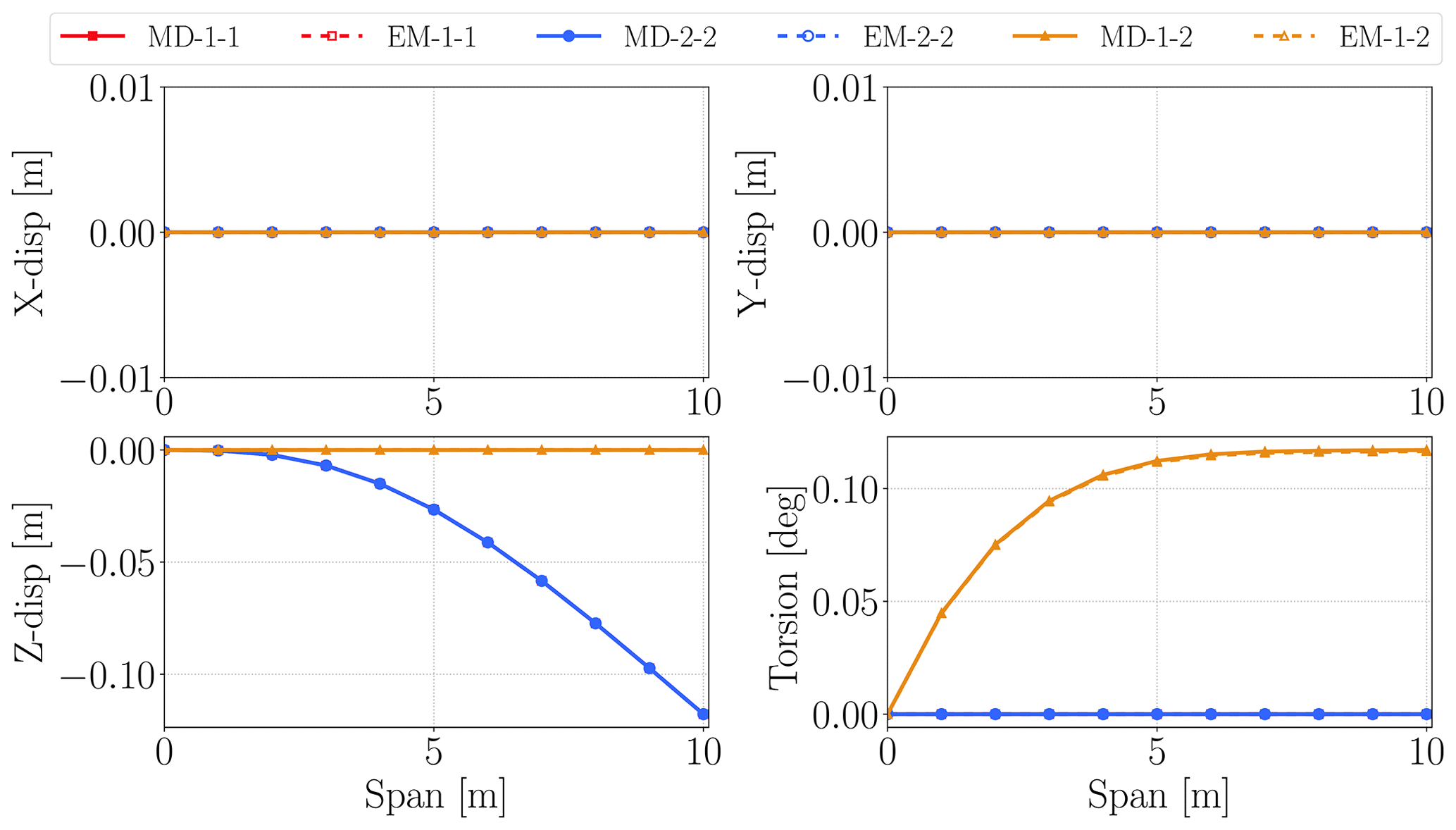
Figure 7 x, y, z and torsion components of modal derivative and expansion mode vectors. Beam span is along the z axis.

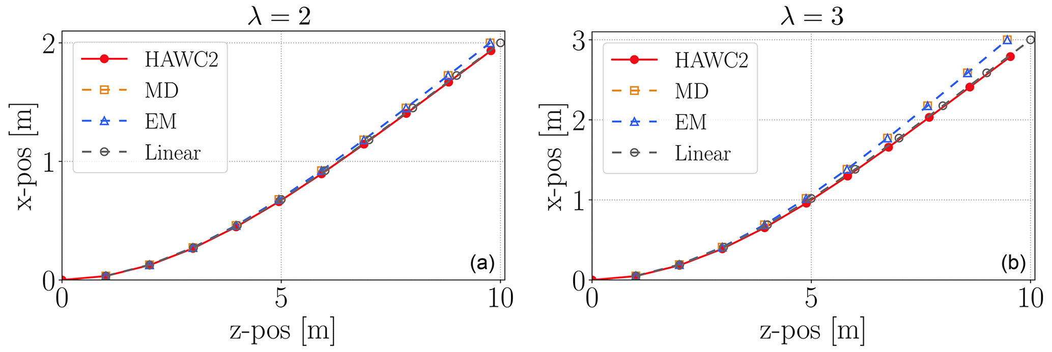
Figure 8 Straight-beam x and z (axial) positions for λ=2 (a) and λ=3 (b) load cases. The positions are shown for HAWC2, linear ROM, MD and EM corrections.

Table 3 Straight-beam lateral (x) and axial (z) tip deflection results for HAWC2, linear model, MD and EM corrections together with the errors in the models compared to HAWC2.

The first test was carried with static loads in the x direction. The applied force vectors are determined from the stiffness matrix (K), first mode shape Φ₁ and amplification factor (λ) as

$$\begin{array}{}\text{(17)}& {\mathbf{F}}_x=\mathit{\lambda }\mathbf{K}{\mathbf{\Phi }}_{\mathrm{1}},\end{array}$$

where mode shape Φ₁ is normalized according to its maximum value.

Expansion mode shape and modal derivative results are the same for this test case; therefore they are given together in Table 3, which shows the tip displacements for the linear ROM without corrections (“Lin.”) and with modal derivative (“MD”) and expansion mode (“EM”) corrections and HAWC2 results. Modal derivative, expansion mode and linear ROM results are the same for lateral (x) deflections, since uncoupled mode shapes result in zero values in lateral-direction components (see Fig. 7) of modal derivative and expansion mode vectors. Linear ROM error in the x direction increases as the deflections increases, and the error is less than 5 % for deflections of 20 % beam length. Moreover the linear model cannot capture any axial (z) displacement, whereas correction factors work quite well. The axial (z) deflection is a secondary effect and is captured by corrections coming from modal derivatives and expansion modes, whereas the linear model estimates zero displacement in the z direction and 100 % error for all solutions. Modal derivative and expansion mode errors are increasing by deflections and are much larger than bending (x) direction errors. The two main sources of error in the secondary (z) direction are truncation errors coming from Eq. (2) and the error in the bending (x) direction, which is even amplified for secondary effects due to the formulation.

Figure 8 shows x and z (axial) positions of the structural nodes computed from HAWC2, linear ROM, MD and EM models for λ=2 and λ=3 load cases. The quadratic corrections capture the secondary effects all along the beam length.

The second test case includes static loads in the x and y directions. The load components are determined by similar formulation given in Eq. (17). The x-force components are amplified by λ=2.5, and the y-force components are amplified by λ=1.0. Figure 9 shows x, y, z displacements and torsion deflections along the beam length. The linear model estimates x and y displacements quite accurately, and quadratic vectors do not alter results in these directions, since they do not have components in these directions (see Fig. 7). On the other hand they capture the secondary effects in the z and torsion directions due to geometric nonlinearities. The linear ROM cannot capture any axial (z) displacements and torsion deflections. On the other hand, MD and EM corrections result in accurate estimation of the secondary effect even though the loads are applied in two directions. Hence, they can also capture the couplings between different directions.

Figure 9 Straight-beam x, y and z displacements and torsion motion results along the beam span. The static load has x and y components.

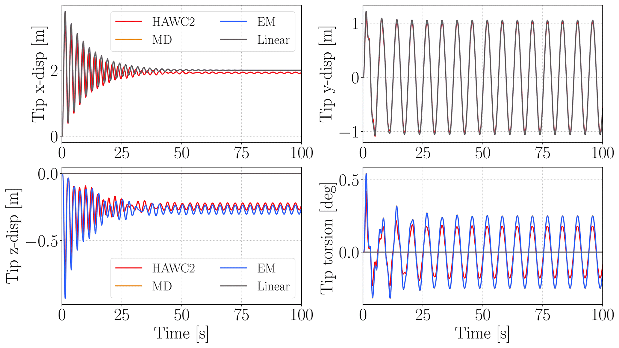
Figure 10 Straight-beam dynamic analysis tip x, y and z displacements and torsion deflections for HAWC2, linear ROM, MD and EM corrections.

The last load case with the straight-beam model includes dynamic loads in two lateral directions. The x-direction load is constant with λ=2, whereas the y-direction load is computed as

$$\begin{array}{}\text{(18)}& {\mathbf{F}}_y\left(t\right)=\mathbf{M}\mathit{g}\sin \left(\mathit{\omega }t\right),\end{array}$$

where M is the mass matrix, g is the acceleration vector and ω is a given rotation frequency of the rotor. Note that the beam does not rotate; only the load varies with the given frequency. So, there is no axial (z) force due to centrifugal effects. For this example the gravity vector has only y acceleration with a value of 9.81 m s⁻², and ω is taken as 1 rad s⁻¹. The simulation time step is 0.01 s.

Figure 10 shows tip x, y and z displacements and torsion deflections for 100 s. The linear model can capture dynamics in the y direction very accurately, and its x-direction results are very close to HAWC2 results without any fluctuations after 60 s, which cannot be captured without nonlinear stiffness terms (Gözcü and Dou, 2020). However these fluctuations are very small compared to the overall displacements in the x direction. On the other hand, linear ROM results are again zero in axial and torsion directions, whereas MD and EM corrections work very well even for the initial transition period. Moreover, there is no phase difference between HAWC2 and MD/EM results, which indicates that the nonlinear stiffness effects are very small for cantilever beams with moderate deflections. The fluctuations in the x direction due to nonlinear stiffness term effects show the limitation of this method even though the fluctuations are very small.

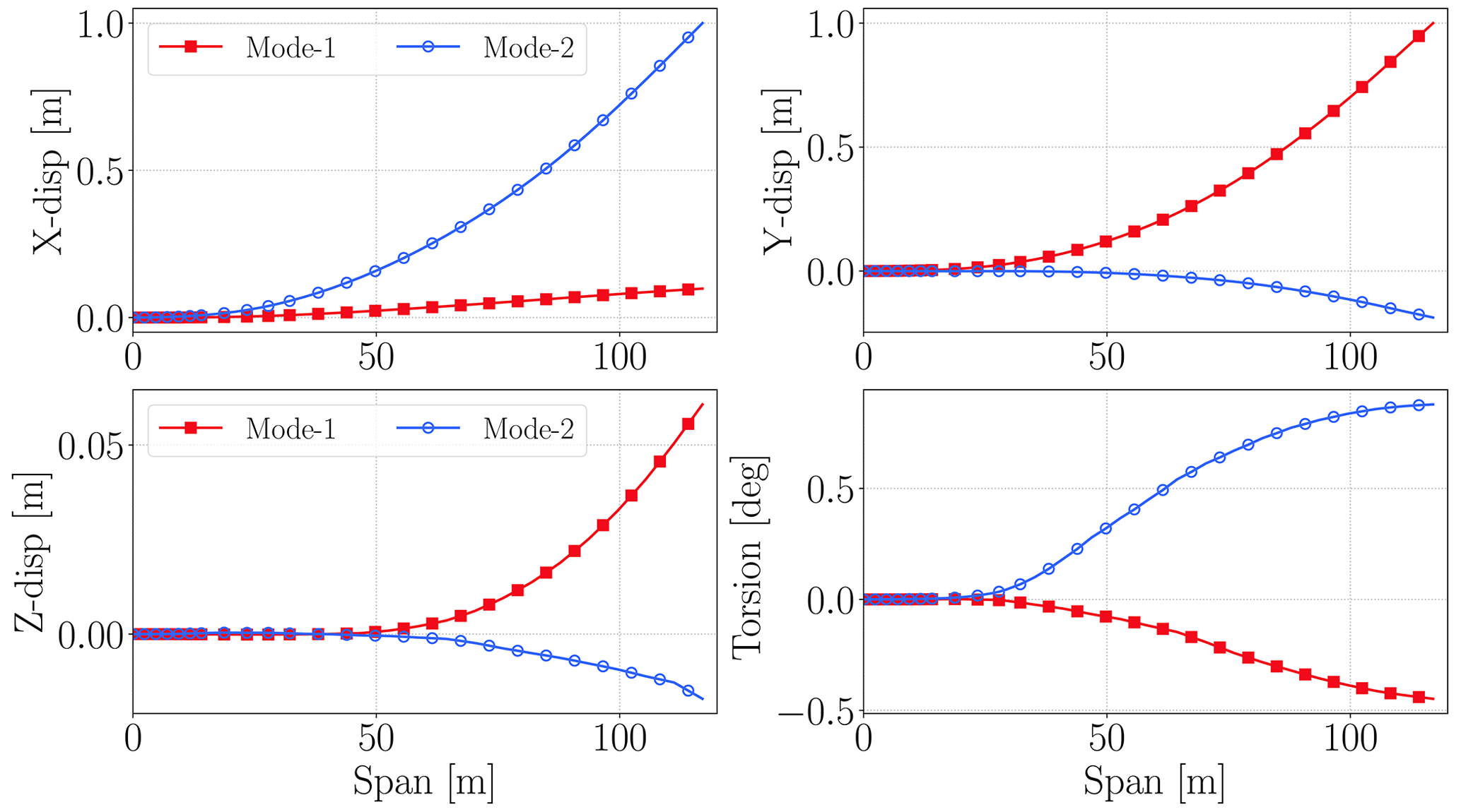
Figure 11 The lateral and torsional displacements of the first two mode shapes of the IEA 15 MW reference wind turbine blade.

4.2 IEA 15 MW turbine blade

The blade of the IEA 15 MW wind turbine is modeled as beams in HAWC2 and FAST for load analysis (Gaertner et al., 2020). It is a more complex structure in comparison to the beam studied in the previous section. The blade has material coupling terms and an initially curved shape due to prebend (mostly in the y direction), aerodynamic twist and being back-swept (mostly in the x direction). Hence, the blade mode shapes are coupled in the x, y, z and torsion directions unlike the straight-beam example. Besides, their cross-section stiffness properties change over the span and material couplings between lateral bending directions, and torsion brings additional couplings in mode shapes. Table 4 shows the relevant blade properties.

Table 4 IEA 15 MW reference wind turbine blade: geometric dimensions, mass, and initial curvature limits in the prebend (y) and twist directions.

The straight-beam example mode shapes are uncoupled so that mode-shape vectors include non-zero values only in one lateral bending direction. However, the mode shapes of the turbine blade are coupled due to its geometry and cross-section material couplings. Figure 11 shows the first two mode shapes of the blade. The first mode shape of the blade is mainly in the y (flapwise) direction with 0.5 Hz, whereas the second mode shape is mainly in the x (edgewise) direction with around 0.7 Hz. Moreover, both mode shapes have components in all directions including the z (axial) and torsion directions. The second mode shape's torsion coupling is much stronger than the first mode shape's coupling, whereas it has weaker coupling in the axial direction than the first mode shape.

Figure 12 shows x, y, z and torsion components of modal derivative and expansion mode vectors for the first two mode shapes. MD and EM vectors are very similar, and they include components in all directions due to the couplings. The difference between MD and EM vectors comes from the numerical computation process. As seen in Sect. 3.2, expansion modes (EMs) are computed via the least-squares method, which uses all displacement and modal amplitude results gathered in matrices, whereas each modal derivative (MD) is computed independently. Since the IEA 15 MW reference wind turbine blade mode shapes are coupled, there are non-zero values at off-diagonal terms in the displacement matrices used during the computation of EMs. This leads to some numerical differences between MDs and EMs for the IEA 15 MW blade case.

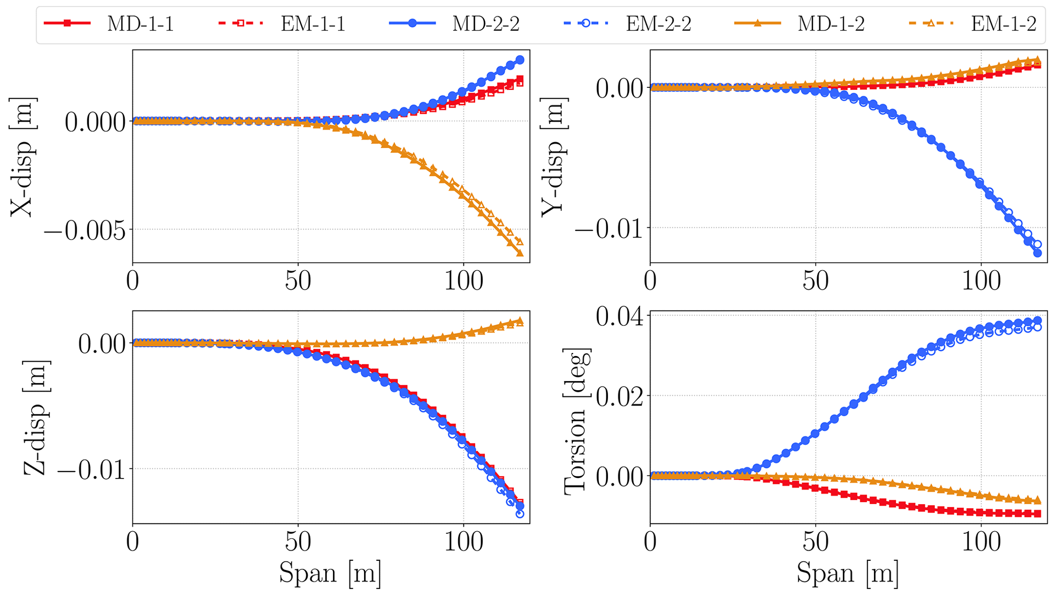
Figure 12 The first three modal derivatives and three expansion modes for the blade of the IEA 15 MW reference wind turbine. The lines show the lateral and torsional displacements along the span of the blade length.

The blade loads include aerodynamic loads at a steady 11 m s⁻¹ wind speed, which gives the highest thrust force. The steady aerodynamic loads for a symmetric rotor (no tilt, no yaw) are time independent (static), and their torsion components are not included for this example so that the torsion due to mode-shape couplings and dynamic forcing is clearer for this example. On top of the aerodynamic loads, the weight of the blade is applied in the x (edgewise) direction with the formulation given in Eq. (18), where ω is 1.0 rad s⁻¹. There are 15 linear mode shapes for the blade ROM, and quadratic vectors for the first three modes are included only, since these modes have very high modal amplitudes among all modes (see Table 5).

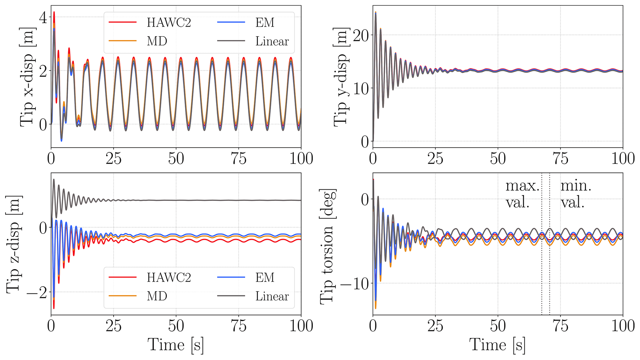
Figure 13 The lateral and torsional displacements for the blade tip of the IEA 15 MW wind turbine obtained by using HAWC2, the linear ROM, MD correction and EM correction.

Table 5 IEA 15 MW blade mean modal amplitude results for last 50 s of the analysis.

Figure 13 shows the tip displacement results of the blade in the edgewise (x), flapwise (y), axial (z) and torsion directions for linear ROM, HAWC2 and correction models. Since most of the thrust force is in the flapwise direction, the largest displacements occur in that direction with a mean displacement around 13.4 m. The fluctuations in the y direction are mostly due to couplings between mode shapes; in other words they are mostly due to linear stiffness effects and not the nonlinear stiffness effects unlike in the case for straight-beam example (see Fig. 10, x-direction results). Since nonlinear stiffness effects are very small in x and y displacements, the results are very similar in terms of magnitude and phase for all models.

Figure 14 Spanwise deflection results at the time when the maximum torsion occurs (67.5 s).

Figure 15 Spanwise deflection results at the time when the minimum torsion occurs (70.66 s).

The secondary effects become clear in the z (axial) and torsion directions. The linear model has 0.84 m mean tip axial displacement for the last 50 s due to mode-shape couplings (see Fig. 11); however the HAWC2 model has −0.41 m mean tip axial displacements for the same time period. Hence, the linear ROM estimates a 2.5 m larger rotor diameter compared to HAWC2. The modal derivative correction model has −0.29 m and expansion mode correction model has −0.23 m mean axial (z) displacements. They also represent the fluctuations in the z directions much more accurately compared to the linear model, which has almost no fluctuations for the last 50 s. The linear model maximum tip torsion error compared to HAWC2 for the last 50 s is about 1.36^∘. The maximum tip torsion errors in MD and EM models for the last 50 s are 0.63 and 0.26^∘. The correction modes also capture the phase of torsion motion more accurately than the linear model, which is out of phase with HAWC2 in the torsion direction. In this study, the load time series are prescribed and not updated with deflection. In other words, the results are not obtained for an aeroelastic analysis. On the other hand, the importance of torsion motion will increase for an aeroelastic analysis. The difference in mean torsion results is critical in static aeroelastic analysis where the steady operating conditions are determined. On the other hand, the difference in torsion fluctuations will affect the damage-equivalent loads (Gözcuü and Verelst, 2020) and aeroelastic stability analysis (Kallesøe, 2011).

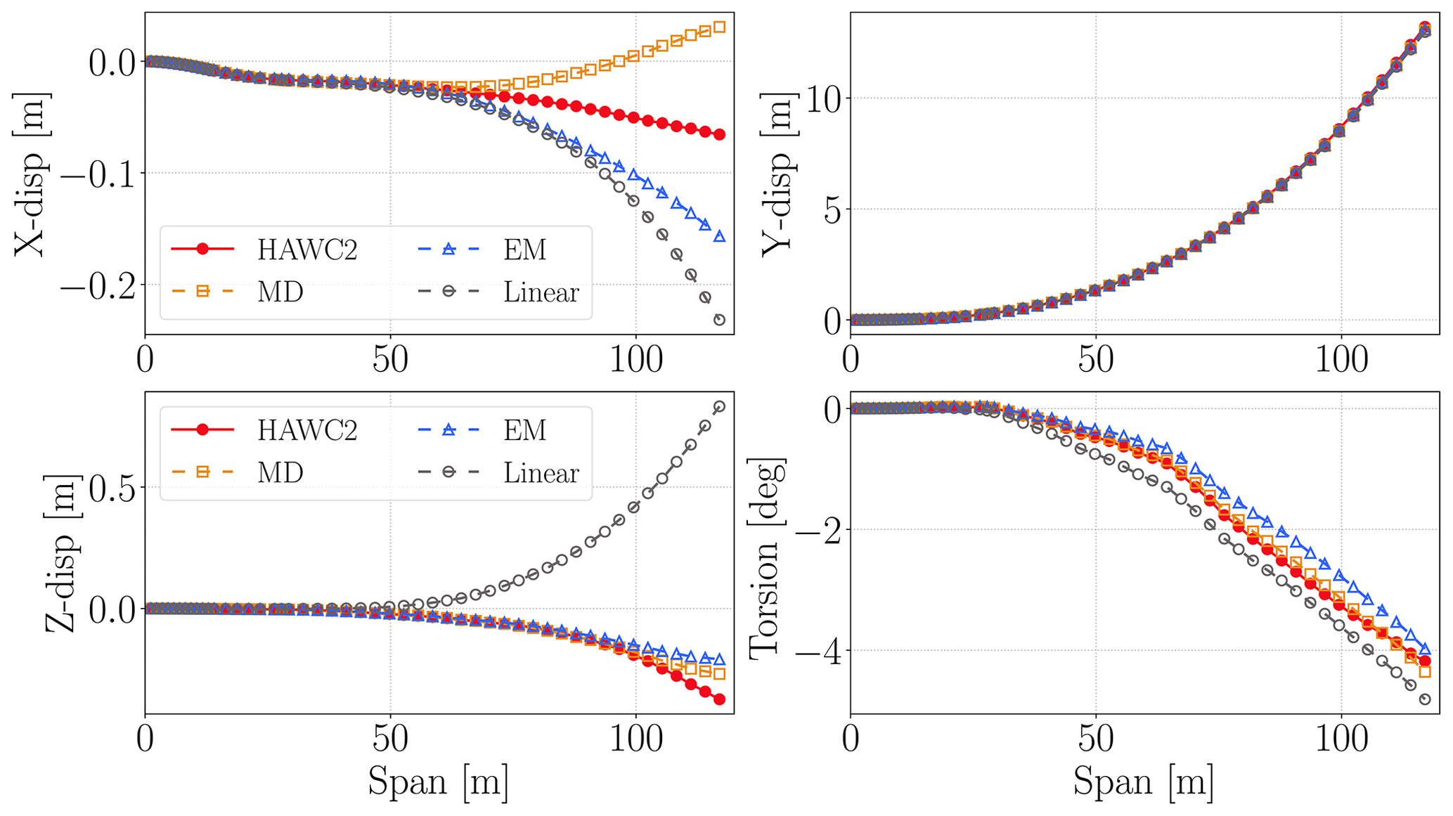
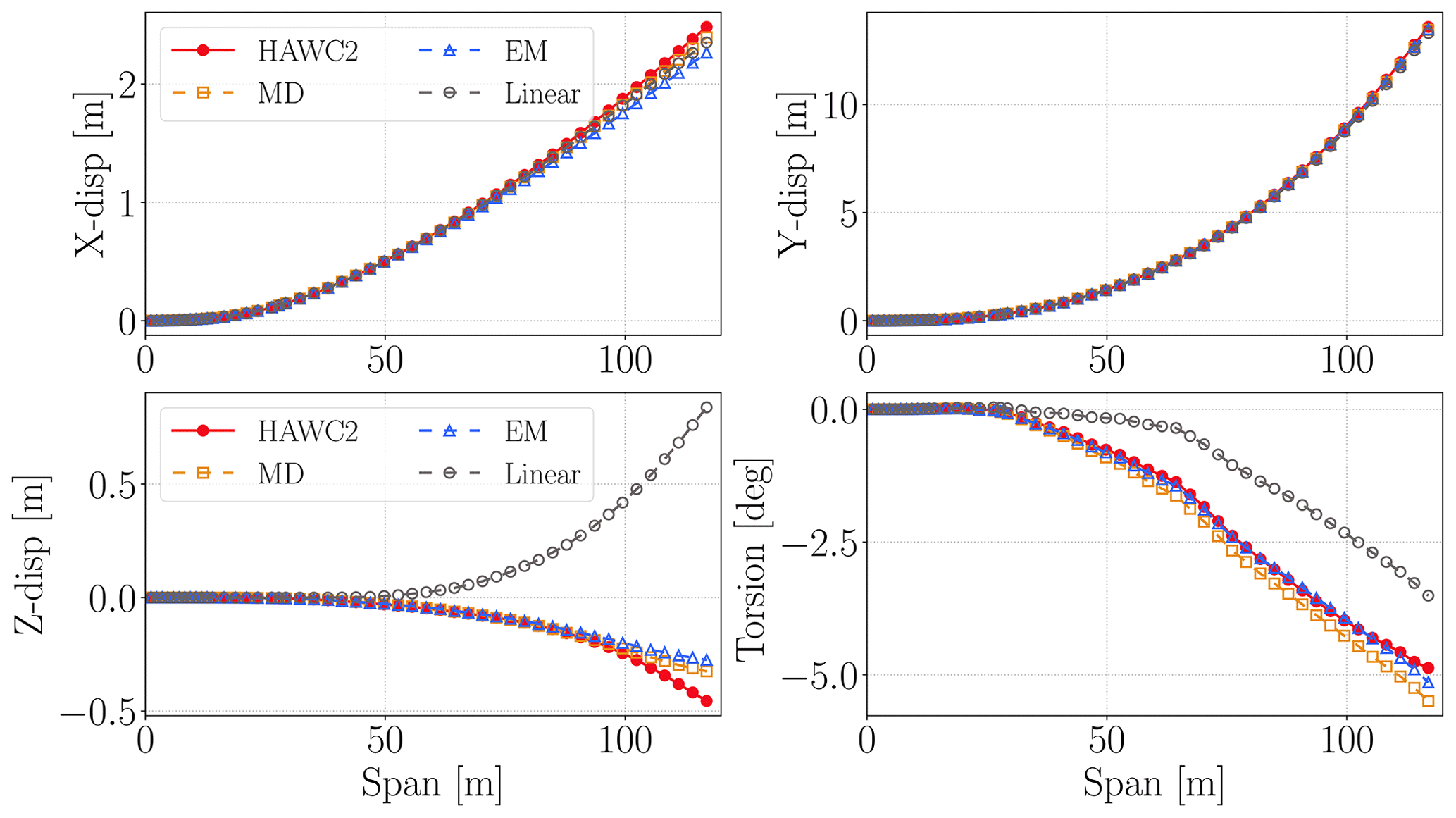
Figures 14 and 15 show the displacement results over the blade span at the two selected time steps where minimum and maximum torsion deflections are obtained in the last 50 s from HAWC2 (shown with dashed black lines). These time steps also correspond to maximum and minimum edgewise displacements. At 70.56 s, where the maximum tip torsion occurs, linear ROM results are quite accurate except z and x displacement (see Fig. 14). On the other hand, MD and EM results are much better than linear ROM results in all directions for that moment. The linear ROM has 1.29 m error in the z direction at the blade tip, whereas MD and EM errors are less than 0.17 m for the blade tip in Fig. 15. The linear ROM predicts a nonphysical elongation in the z direction because of the non-zero motion in the z direction in the linear mode shapes (particularly “Mode-1”) shown in Fig. 11. In contrast, the two correction methods in this study are not limited by the linear mode shapes. Both of the correction methods provide a correct estimation of the shortening of the blade in the axial direction.

Figure 14 shows displacement and torsion results along the blade span at the maximum tip torsion moment (67.51 s in Fig. 13). The linear ROM is quite accurate in the x and y directions; however it has low accuracy in the z and torsion directions. Its total torsion error over the blade span is 33.6^∘, whereas MD error is 7.7^∘ and EM error is 1.7^∘ along the blade span compared to HAWC2 results. The z-direction results are similar to minimum-torsion-moment results in Fig. 15.

One of the findings in Figs. 10 and 13 is that the frequency of the vibration is not affected by the large deflections of the blade. Even the linear model can predict the vibration frequency or the time period of the periodic response in good agreement with HAWC2 simulation in the main deflection directions. In practice, this means that no correction is needed for the vibration frequency in the case of large deflections. This also suits the application of the proposed correction method to a variety of slender cantilever structures including wind turbine blades. Besides, this allows using correction terms to capture secondary effects due to geometric nonlinearities for moderately large deflections.

5 Conclusions

This study introduced a correction approach for capturing the geometric nonlinear effects in the reduced-order models of cantilever beam structures which go through moderately large deflections. The approach is examined based on two different types of correction vector (i.e., the modal derivatives and expansion modes), leading to similar results. Both correction vectors can be pre-computed by using a geometrically nonlinear beam solver and then used in the dynamic response analysis. The advantage of this approach is its low computational cost during the coupled response analysis. It is suitable for integration into the aeroelastic analysis tools that use the modal-based reduced-order models for the cantilever beam structures such as wind turbine blades and airplane wings.

The proposed method is demonstrated by using two case studies, including a simple cantilever beam and the blade for the IEA wind 15 MW reference turbine. For the simple cantilever beam, its mode shapes are uncoupled in the sense that the displacements in the two bending modes are orthogonal to each other. For the turbine blade, its mode shapes are coupled because of its curved and twisted geometry and complex cross-sectional properties. In the case study of the simple cantilever beam, the correction vectors based on the modal derivatives and expansion modes have identical results and they captured geometrically nonlinear effects accurately for the lateral deflections for up to 25 % of the beam length. In the case study of the blade of the IEA 15MW reference turbine, modal derivative and expansion mode vectors have small deviations from each other, since they are computed by different numerical processes. The blade axial displacements estimated by the linear ROM are in the opposite direction to the axial displacements in the HAWC2 results. In other words, the linear ROM predicts a nonphysical elongation of the IEA 15 MW blade span for the given load case. In contrast, the two correction vectors in this study give a good estimation of the axial motion of the blade tip. Further, the torsion displacements obtained by the linear ROM are out of phase with the HAWC2 results, whereas the torsion displacements obtained by using the two correction vectors in this study are in phase with the HAWC2 results. The torsion phase difference between the nonlinear solver HAWC2 and the linear ROM is crucial for aeroelastic stability and load analysis of wind turbine blades. The comparison of these results shows that the proposed correction method is capable of accurately estimating the nonlinear dynamic response of the cantilever beam structures with large bending deflections, and it is also suitable for the wind turbine blades with curved and twisted geometry and complex cross-sectional properties.

The study can be extended with an implementation of the correction method into an aeroelastic tool that uses the reduced-order models for airplane wings or wind turbine blades. Further, the proposed correction method can also be implemented based on machine learning methods such as neural network models or adaptive kriging methods.