the Creative Commons Attribution 4.0 License.
the Creative Commons Attribution 4.0 License.
 | 12 Oct 2023
Revealing inflow and wake conditions of a 6 MW floating turbine
Jakob Mann
Camille Dubreuil-Boisclair
We investigate the characteristics of the inflow and the wake of a 6 MW floating wind turbine from the Hywind Scotland offshore wind farm, the world's first floating wind farm. We use two commercial nacelle-mounted lidars to measure the up- and downwind conditions with a fixed and a scanning measuring geometry, respectively. In the analysis, the effect of the pitch and roll angles of the nacelle on the lidar measuring location is taken into account. The upwind conditions are parameterized in terms of the mean horizontal wind vector at hub height, the shear and veer of the wind profile along the upper part of the rotor, and the induction of the wind turbine rotor. The wake characteristics are studied in two narrow wind speed intervals between 8.5–9.5 and 12.5–13.5 m s−1, corresponding to below and above rotor rated speeds, respectively, and for turbulence intensity values between 3.3 %–6.4 %. The wake flow is measured along a horizontal plane by a wind lidar scanning in a plan position indicator mode, which reaches 10 D downwind. This study focuses on the downstream area between 3 and 8 D. In this region, our observations show that the transverse profile of the wake can be adequately described by a self-similar wind speed deficit that follows a Gaussian distribution. We find that even small variations (∼1 %–2 %) in the ambient turbulence intensity can result in an up to 10 % faster wake recovery. Furthermore, we do not observe any additional spread of the wake due to the motion of the floating wind turbine examined in this study.
- Article
(8661 KB) - Full-text XML
- BibTeX
- EndNote


The increase in the global renewable energy capacity is largely based on the continuation of the current expansion rate of the wind energy sector and the reduction in the associated production costs (Wiser et al., 2021). To fill this increased capacity, wind turbines and wind farms will continue to increase in size, with a growing focus on offshore wind energy production. Despite the operational challenges that wind turbines encounter in offshore conditions, several factors favor offshore deployment: the size of the available areas, the generally strong wind, and the spatial homogeneity of wind conditions. In order to optimize the energy production of both onshore and offshore wind farms and to ensure that they are operational during their expected lifetime, it is necessary to be able to realistically model intra- and inter-farm flows, e.g. the individual wakes, the blockage in front and speed-up around the wind farms, and the wind farm wake. In the case of intra-farm flows, the wind turbines are typically located in the far wake of adjacent wind turbines, where the characteristics of the flow are mainly related to the ambient wind conditions, which are usually described by the inflow speed, shear and veer profiles, turbulence intensity, atmospheric stability, and surface roughness. A thorough review of the current state-of-the-art physical description of those flows is presented in Porté-Agel et al. (2020), who highlights the importance of a realistic physical parameterization of the flow in the far wake to enable accurate prediction of the wind turbine production and the wind-induced loads. The impact of atmospheric conditions on wake properties is investigated in numerical studies (e.g. Wu and Porté-Agel, 2012; Rodrigues et al., 2015) and wind tunnel experiments (e.g. Chamorro and Porté-Agel, 2009, 2010). For example, the results of such studies have formed our current knowledge that an increase in turbulence intensity results in a faster wake recovery and that stable atmospheric stratification favors the downwind propagation of the wake trace.
Due to the varying sea depth of the exclusive economic zone of coastal countries and the wind farm construction restrictions regarding the minimum distance from land, floating wind turbines will often be an attractive option for the development of offshore wind farms. In the case of floating wind turbines, the motion that results from the interaction of the floating structure with the wind and sea has to be considered in addition to the atmospheric conditions. The wake characteristics of floating wind turbines have been studied using numerical (Wise and Bachynski, 2020; Kleine et al., 2022; Nanos et al., 2022; Chen et al., 2022; Li et al., 2022) and wind tunnel (Fu et al., 2019; Schliffke et al., 2020) experiments. Those studies focused on the impact of the sway (Fu et al., 2019; Nanos et al., 2022; Li et al., 2022), surge (Fu et al., 2019; Schliffke et al., 2020; Chen et al., 2022), and heave (Kleine et al., 2022) motions on the turbine operation. Yet, the absence of the study of the motion of floating turbines under realistic atmospheric turbulence conditions limits our understanding of how the impact of the motion of the wind turbine on the wake properties can be utilized in control strategies that optimize the operation of wind turbines and subsequently wind farms.
In this context the conduction of field campaigns is necessary for increasing our knowledge about the physics that govern the wake flow. In this respect, the development of remote sensing sensors based on the light detection and ranging (lidar) technique has extended the study of wake flows generated by full-scale wind turbines in the atmospheric boundary layer. This was achieved since their design enables the acquisition of wind observations with high spatial and temporal resolution while operating either ground based (e.g. Iungo et al., 2013; Iungo and Porté-Agel, 2014; Archer et al., 2019; Menke et al., 2020) or nacelle mounted (e.g. Bingöl et al., 2008; Aitken et al., 2014; Aitken and Lundquist, 2014; Carbajo Fuertes et al., 2018; Schneemann et al., 2021; Cañadillas et al., 2022; Brugger et al., 2022). Wind lidars are now used to detect the propagation of the wake trace (Archer et al., 2019) and, subsequently, measure both the mean (Iungo et al., 2013; Iungo and Porté-Agel, 2014; Menke et al., 2020) and the dynamic (Carbajo Fuertes et al., 2018) wake characteristics. Thus, they are used to evaluate the accuracy of different wake models (Trujillo et al., 2011; Trabucchi et al., 2017; Brugger et al., 2022). Furthermore, the capability of scanning wind lidars to acquire long-range measurements (1–3 km) enables the investigation of the far-wake region while being installed on the ground and the nacelle of wind turbines (Archer et al., 2019; Carbajo Fuertes et al., 2018; Brugger et al., 2022).
In this study, we use two wind Doppler lidars installed on the nacelle of a floating wind turbine that is part of a small offshore wind farm with five wind turbines. Using two lidars enables the synchronous monitoring of the up- and downwind conditions. Thus it was feasible to acquire observations of the characteristics of the wake and relate those to the inflow wind statistics. Similar studies using nacelle-mounted lidars have been performed on onshore wind turbines focusing on wake model validation (Carbajo Fuertes et al., 2018) or investigating the relationship between the wake meandering and the fluctuations in the transverse wind component (Bingöl et al., 2008; Trujillo et al., 2011; Brugger et al., 2022).
Here we present, to our knowledge, the first combined inflow and wake measurements of a floating offshore wind turbine using two nacelle-mounted wind lidars. In Sect. 2, we describe the field campaign and the measuring configuration of the two wind lidars as well as the data post-processing steps. In Sect. 3, we present the two models used to describe the acquired wind lidar measurements in the up- and down-wind directions based on the characteristics of the free and wake flow. Finally, we present our results in Sect. 4 where the accuracy of both the up- and the down-wind wind lidar is assessed, the properties of the mean free wind field are estimated, and the wake flow characteristics are quantified for different inflow wind cases.
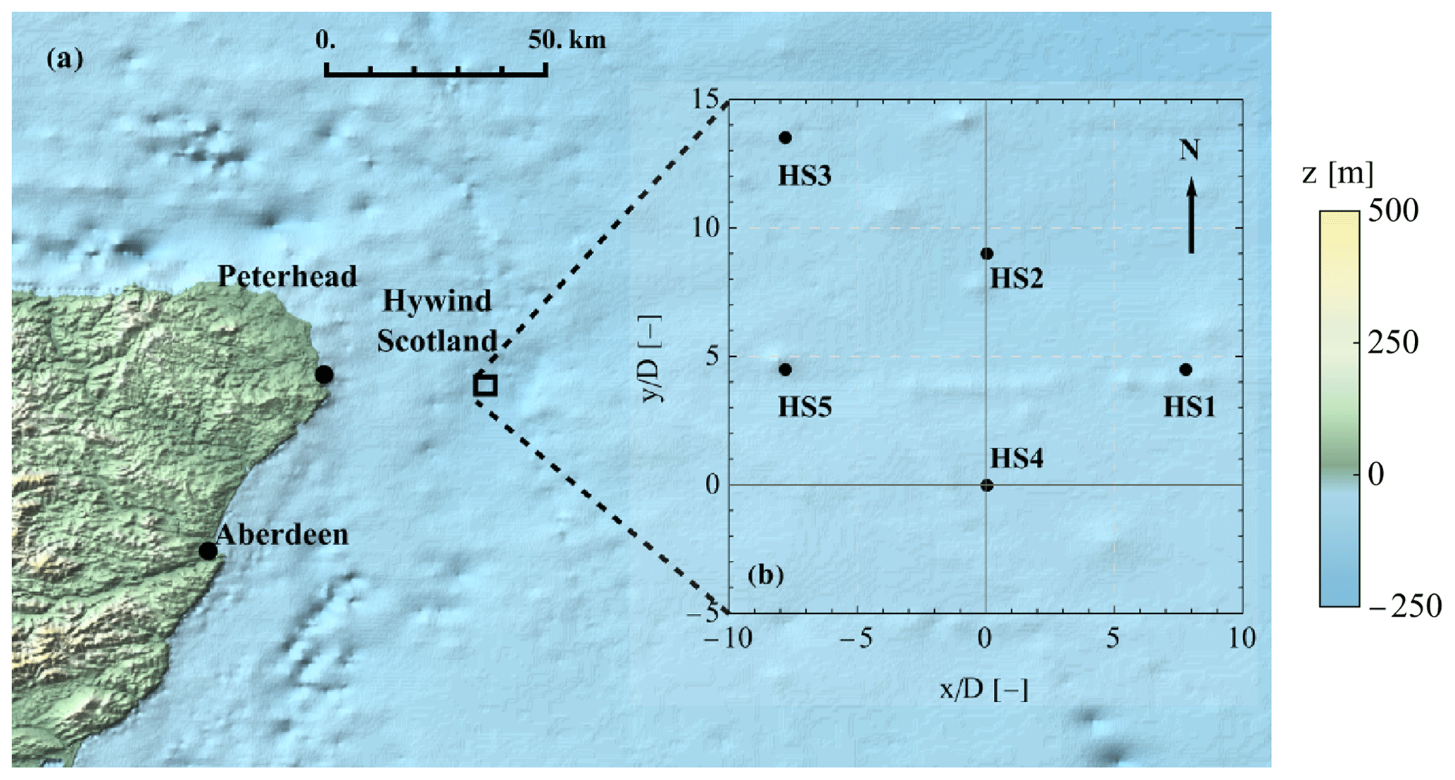
Figure 1(a) Map of the eastern coast of Scotland where the offshore Hywind Scotland wind farm is located (black rectangle). (b) Drawing of the wind farm layout consisting of five wind turbines (denoted as HS1, HS2, HS3, HS4, and HS5) using a right-handed coordinate system where the y axis is aligned to the north, and the origin is placed at the location of the wind turbine (HS4).
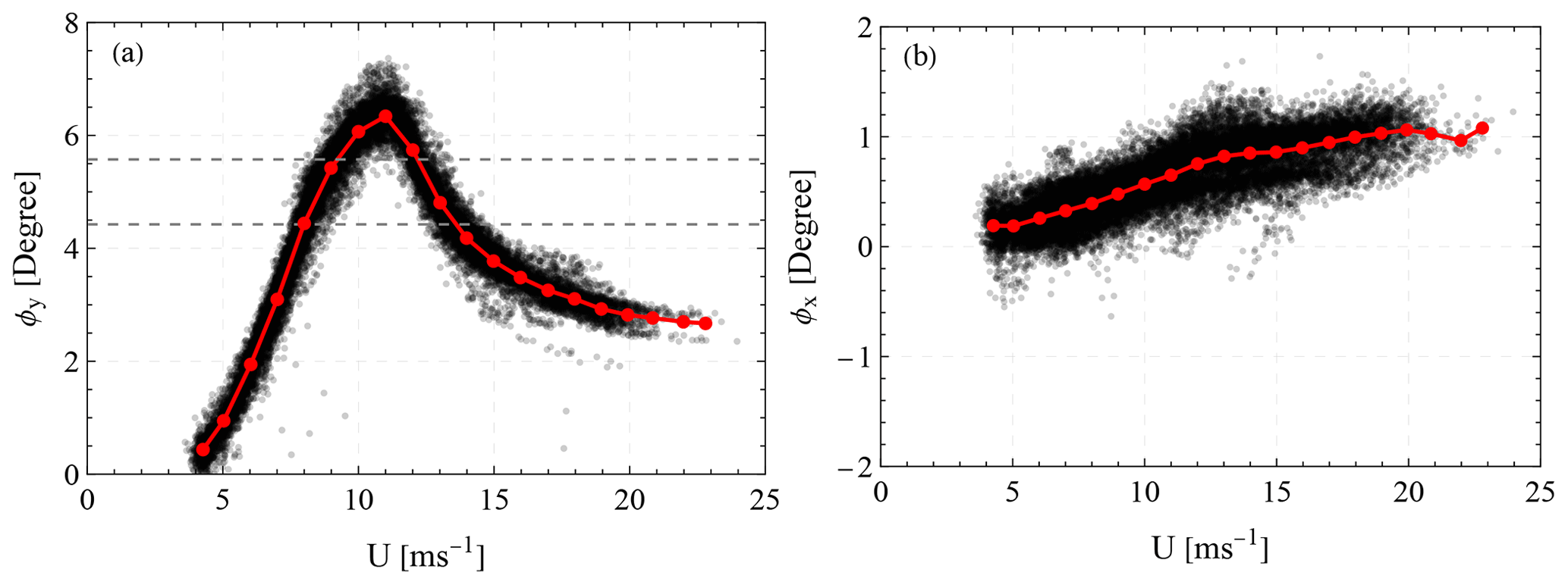
Figure 2(a) Pitch ϕy and (b) roll ϕx values of the HS4 wind turbine for different wind inflow speeds U. The data presented in black correspond to the mean measurements of the MRU installed on the nacelle over a 2 min period. The red line depicts the mean value of the pitch and roll angles per wind speed. The dashed gray lines in the pitch plot highlight the interval used in the analysis of this study (see more in Sect. 4.3).
Hywind Scotland is the world's first commercial floating offshore wind farm. It is located approximately 26 km from the east coast of Scotland (see Fig. 1a). In total, five Siemens Gamesa SWT-6.0-154 turbines with a hub height H=98.6 m, a rotor diameter D=154 m, and a rotor rated speed of ∼10 m s−1 are mounted on a ballast floating platform (Jacobsen and Godvik, 2021). The blade pitch is controlled as a conventional bottom-fixed wind turbine during operation below the rated wind speed. However, above the rated wind speed the blade pitch control system interacts with a floater motion control system. The closest distance between neighboring wind turbines is approximately equal to 1387 m (9 D). The wind turbines' (denoted as HS1, HS2, HS3, HS4, and HS5) locations form a “W”-shape layout, with a clockwise rotation of 30∘ in relation to the north, as shown in Fig. 1b. The layout is presented in a right-handed coordinate system whose y axis is aligned to the north, and the origin is the location of the HS4 wind turbine. The HS4 wind turbine was instrumented with two nacelle-mounted wind lidars: a Wind Iris lidar by Vaisala Oyj (Finland) to measure the inflow and a G4000 Galion lidar by SgurrEnergy (Scotland) to measure the wake. The two wind lidars operated for a period of 3.5 months between June and September 2020. During this period, an additional G4000 Galion wind lidar was installed on the HS2 wind turbine to measure downwind relative to the turbine. Both HS2 and HS4 wind turbines were further instrumented with a motion reference unit (MRU) to monitor the motion of the nacelle. The MRU measured the angles of rotation about the longitudinal and transverse axes in relation to the yaw direction of the turbine. The data acquired from the MRU were logged by the supervisory control and data acquisition (SCADA) system at 1 Hz. Figure 2 presents the pitch ϕy and roll ϕx angles averaged over a period of approximately 2 min as a function of the mean horizontal wind speed U. The 2 min period was selected in order to study the response of the wind turbine over a period that was similar to the duration of the wake scan performed by the G4000 Galion wind lidar (see more in Sect. 2.1). The mean pitch corresponds to a rotation about the transverse axis relative to the yaw direction and the roll about the longitudinal axis.
We observe that both the pitch and roll angles depend on the wind speed. The pitch angle has an increasing trend with wind speed, reaching approximately 7∘ at 11 m s−1 (slightly higher than the rotor rated speed), followed by a decrease down to 3∘. Positive pitch angles indicate a counterclockwise rotation of the rotor plane. The decrease to 3∘, which is observed when the wind is higher than the rotor rated speed, is attributed to a decrease in the thrust exerted on the wind turbine's rotor due to the pitch of the wind turbine's blades. The roll angle shows a constant and slightly increasing trend with increasing wind speed, which on average varies between 0 and 1∘, balancing the torque of the rotor. Jacobsen and Godvik (2021) studied the dynamic response of the wind turbines at Hywind Scotland and found an increase in the standard deviation of both the pitch and the roll angle with an increasing wind speed. However, up to mean wind speeds of 20 m s−1, those variations are normally less than 1∘, indicating that the response of the floating platform is very stable.
2.1 Wind lidars
The two nacelle-mounted wind lidars used for this study are the Wind Iris and the G4000 Galion monitoring the upwind and downwind conditions, respectively, and both are pulsed Doppler wind lidars. Doppler wind lidars measure the radial speed which corresponds to the projection of the wind vector on the line of sight of a laser beam. In the case of the Wind Iris, radial wind speed measurements are acquired over four fixed line of sights, which form the corners of a rectangle at any measuring distance. In our study, radial wind speeds were measured at a sampling rate of 0.25 Hz in 10 separate range gates corresponding to the upwind distances 50 m (0.32 D), 80 m (0.52 D), 120 m (0.78 D), 160 m (1.04 D), 200 m (1.30 D), 240 m (1.56 D), 280 m (1.82 D), 320 m (2.08 D), 360 m (2.34 D), and 400 m (2.60 D), when the Wind Iris was leveled. The first seven range gates were located within the swept area of the wind turbine, while the last three were located outside the rotor plane with respect to the transverse direction (see Fig. 3, red dots). The four telescopes that define the measuring geometry are enclosed in a single module installed 4.5 m above the rotor center, which is 103.4 m a.s.l. (above sea level), and 4 m behind the rotor plane. Furthermore, the telescope of the Wind Iris was tilted by 2.5∘ with respect to the horizontal plane to bring the center of the measuring plane to hub height at a distance of 2.5 D, when the wind turbine was not operating.
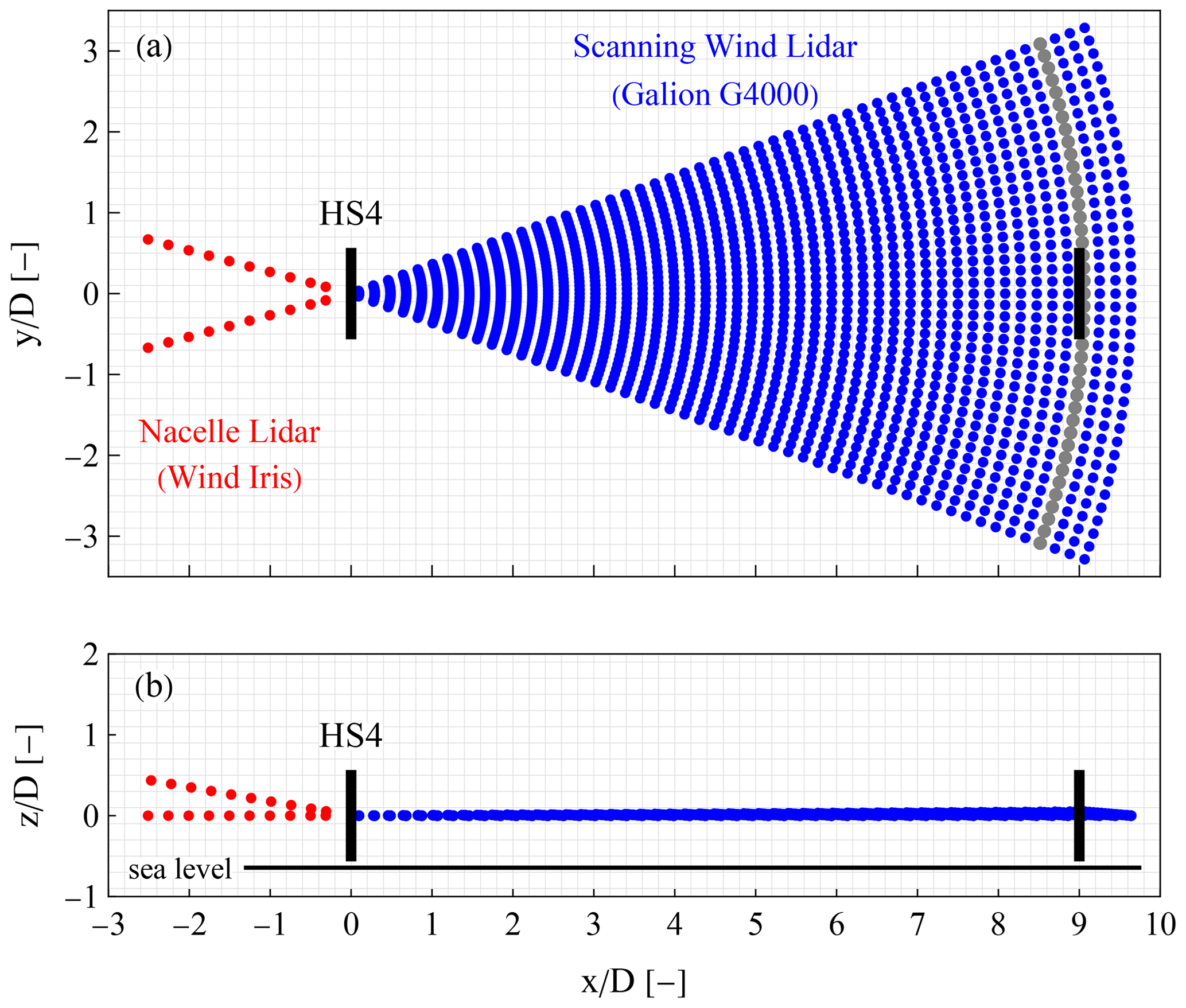
Figure 3Top (a) and side (b) view of the measuring configuration used to monitor the up- and downwind flow relative to the HS4 wind turbine when the pitch of the rotor is equal to 5∘. The scanning pattern of the G4000 Galion is presented with blue dots and the measuring locations of the Wind Iris with red dots. The coordinate system is defined such that the x axis is aligned with the downwind direction relative to the wind turbine, and its origin is located at the wind turbine's rotor. The figure also depicts the expected position of the rotor of the HS1, HS2, and HS5 wind turbines when the yaw of the HS4 was equal to 120, 180, or 240∘ (black line at 9 D). The gray arc highlights those range gates, where the rotor of the HS1, HS2, and HS5 wind turbines is expected to be located when the yaw direction of the HS4 is within the 100–140, 160–200, and 220–260∘ ranges.
The G4000 Galion mounted on the HS4 wind turbine is a pulsed Doppler lidar where a scanner controls the direction of the beam. This lidar was configured to do a plan position indicator (PPI) scan. The PPI scan consisted of 41 line-of-sight measurements spanning from −20 to 20∘ in the azimuthal direction and had a duration of approximately 2 min. Each line-of-sight measurement consisted of 50 range gates that extended from 15 to 1485 m (9.6 D), which were sampled at 0.32 Hz. The 0.32 Hz was chosen in order to ensure high data availability along the measuring range. Furthermore, the PPI scan was performed with an elevation angle of 5∘. This elevation angle was selected to compensate for the pitch angle of the wind turbine's nacelle so that the scan was horizontal when the mean wind speed was between either 8.5–9.5 or 12.5–13.5 m s−1; see Fig. 2a. The pulsed scanning Doppler lidars have the advantage that they can acquire instantaneous measurements along a beam with a fixed spatial resolution. However, the required pulse accumulation time for producing reliable estimates of the radial speed limits the scanning speed, especially when measurements at long ranges are required. For these reasons, the PPI scan duration of 2 min was chosen, followed by 26 s of resetting the scanner head to its initial position. Thus, approximately 12 scanning patterns were acquired per 30 min period, which was the time period used in the wake analysis (see more in Sect. 4.3.2). The measurements were grouped in a Cartesian grid whose x axis was aligned with the downwind direction parallel to the yaw direction of the wind turbine, with an origin at the center of the wind turbine's rotor. The grid consisted of three-dimensional cells with dimensions . The size of the cells was determined by the length of the range gates (30 m) and resulted in having at least one measurement per grid cell per scanning pattern (see Fig. 3a).
2.2 Post-processing of wind lidar data
Prior to the lidar data analysis, a quality check was performed in order to minimize biases that could originate from erroneous radial speed measurements. We present the post-processing of the two lidar data sets separately in the following two subsections.
2.2.1 Wind Iris wind lidar
In the analysis of the Wind Iris measurements, only the data flagged with a valid radial wind speed estimation were used. These data were selected based on the Radial Wind Speed Status index (RWS Status index), a parameter that is provided by the Wind Iris, which describes the quality of the radial wind speed estimation of each measurement (for more information we refer to the Wind Iris user manual; Avent Lidar Technology, Version 2.1.1). However, it was observed that on 84 % of the 1 h periods examined, on average 0.2 % erroneous estimations of the radial wind speed still remained after the valid data selection. Due to this, an additional filtering was applied, in which values outside the lower and upper outer statistical fences of the time series were treated as outliers for each 1 h period. The fences were defined by the first (lower fence) or third (upper fence) quartiles minus (lower fence) or plus (upper fence) 1.5 times the interquartile range of the distribution of the radial wind speeds per period per range gate. The highest signal-to-noise ratio (SNR) values in all four line of sights were found approximately at 200 m, corresponding to the range where the Wind Iris has the highest sensitivity, and thereafter it decreased linearly (in dB) with distance. The corresponding data availability (defined here as the ratio between the selected and total acquired data) varied between 90 % and 70 %, with a decreasing trend for increasing measuring distance. In addition, the two lower beams presented a slightly lower availability compared to the two upper beams, which could be attributed to blade blockage.
2.2.2 G4000 Galion wind lidar
As described in Sect. 4.3, the G4000 Galion wind lidar data were filtered for cases where the PPI scans were leveled. The data filtering was based on the intensity values provided by the Galion software (SgurrEnergy Ltd., Galion Toolbox, User manual Revision 2017 B3), according to which the lower threshold value of 1.01 is recommended as the lower acceptable threshold for a valid measurement. This value corresponds to an SNR of −20 dB. Even though this is a conservative threshold, in relation to the ones typically used in profiling (e.g. −29 dB in Gryning and Floors, 2019) and scanning (e.g. −24 dB in Menke et al., 2020) wind lidars, adequate data availability was observed in the acquired data set. In addition, in order to exclude erroneous wind estimations that were observed mainly in the closest and furthest range gates, an additional filter was constructed following the same method as the one applied to the Wind Iris data to detect outliers.
The parameterization of the upwind and downwind conditions was performed using a right-handed coordinate system whose x axis was anti-parallel to the axis normal to the rotor plane and thus aligned to the mean downwind direction in cases with no yaw misalignment. Furthermore, we denote the three-dimensional wind vector , where u1 is the component aligned with the x direction. Using Reynolds decomposition, we express each of the three components as the sum of a mean (denoted with an overbar symbol) and a fluctuating (denoted with a prime symbol) component: .
3.1 Upwind radial speed model
The parameterization of the inflow wind conditions was performed by assuming the following:
-
the two components of the horizontal mean wind speed , , at a given height, are horizontally homogeneous within each measuring distance;
-
the vertical wind component is negligible ( m s−1);
-
the wind shear and veer within the vertical range of the measuring area of the nacelle lidar are constant with height.
The first two aforementioned are justified by the horizontal homogeneity of the offshore mean wind field. The third assumes that in the vertical range between 68–138 m (where the Wind Iris measurements are acquired), non-linearities in the wind profile are weak at the measurement height (Peña et al., 2009). Based on the above assumptions, the mean wind vector U in any given location with coordinates (x, y, z) can be expressed only as a function of height z as
where and are the mean free horizontal velocities at the height of the Wind Iris (103.4 m), and and are the vertical gradients. The wind component u is not expected to be homogeneous along the streamwise direction due to the induction by the wind turbine. We express this blockage effect using the induction factor a that characterizes the reduction in the longitudinal wind speed along a line normal to the center of the rotor, based on the vortex sheet theory (Conway, 1995; Medici et al., 2011). This can adequately describe the wind speed evolution as it approaches a wind turbine rotor, as demonstrated in a field test by Simley et al. (2016) in the case of an onshore wind turbine, using the following formula:
where is the distance normalized by the rotor radius R=77 m. Here, it is also assumed that the induction effect does not induce a spatial variability of the transverse component of the wind and that the induction is independent of y and z for the positions of the range gates. These simplifying approximations are judged to be reasonable compared to the full expressions of Conway (1995).
Based on the above considerations the wind vector of Eq. (1) can be rewritten as
where
describes the expected reduction in the longitudinal speed across the whole rotor area, and xL is the distance between the rotor plane and the nacelle lidar (i.e. 4 m). Such parameterization formulations of the radial speed of a wind lidar have also been used in other studies of nacelle-mounted wind lidars (e.g. Borraccino et al., 2017).
The Wind Iris acquires radial wind speed νr measurements in four different upwind directions, which correspond to the projection of the wind vector U onto the unit vector of each of the line of sights of the wind lidar:
where is the three-dimensional unit vector, and the superscripts i=1, 2, 3, 4 denote the index of each beam. The unit vector n, which is defined by both the azimuth ϕ and the elevation θ angles of the line of sight, and by the pitch ϕy and roll ϕx angles of the wind turbine's nacelle, is equal to
where is equal to
where ∘ and ∘ depending on the line-of-sight direction.
Equation (5) can be written as
is the matrix of the line-of-sight unit vectors, and df is the distance from the instrument to the measurement volume. In the Wind Iris data, for each beam, an upwind distance xf is reported, which is the nominal x distance from the instrument. Thus, df can be computed by multiplying xf by the norm of the vector .
The estimation of the upwind parameters , , , and of the induction factor a was performed by solving Eq. (8). The solution was found using a non-linear model solver in Mathematica (Wolfram Research), based on the 10 min mean values of the radial speeds in all available range gates. The solver had as input the initial estimation of the wind conditions using only the radial wind speed measurements acquired in the furthest available range gate per 10 min period. In this analysis, we have selected only the 10 min periods with a radial speed availability larger than 50 %. The performance of the model, in estimating the upwind mean wind speed characteristics, is investigated through the calculation of the root mean square error (hereafter denoted as εu) between the modeled and measured radial wind speeds, for each 10 min period.
3.2 Wake radial speed model
The study of the wake characteristics was performed by expressing the radial wind speed as a function of both the upwind conditions (mean wind speed and direction) and the corresponding wind speed deficit that propagates downwind from the wind turbine, using the following expression:
where νr is the radial wind speed measurement acquired by the scanning wind lidar in different longitudinal x and transverse y distances in relation to the center of the rotor, is the mean free speed of the horizontal wind at the height of the wind lidar, ϕ is the azimuth angle of the line of sight of the scanning wind lidar equal to , γ is the mean wind direction relative to the yaw of the wind turbine equal to , σ(x) is a parameter representing the spread of the wake, yo(x) is the center of the wake defined by the location of the maximum wind speed deficit in the transverse direction at any downwind distance, y is the transverse coordinate relative to the center of the rotor, and β(x) is a scaling parameter representing the wind speed deficit.
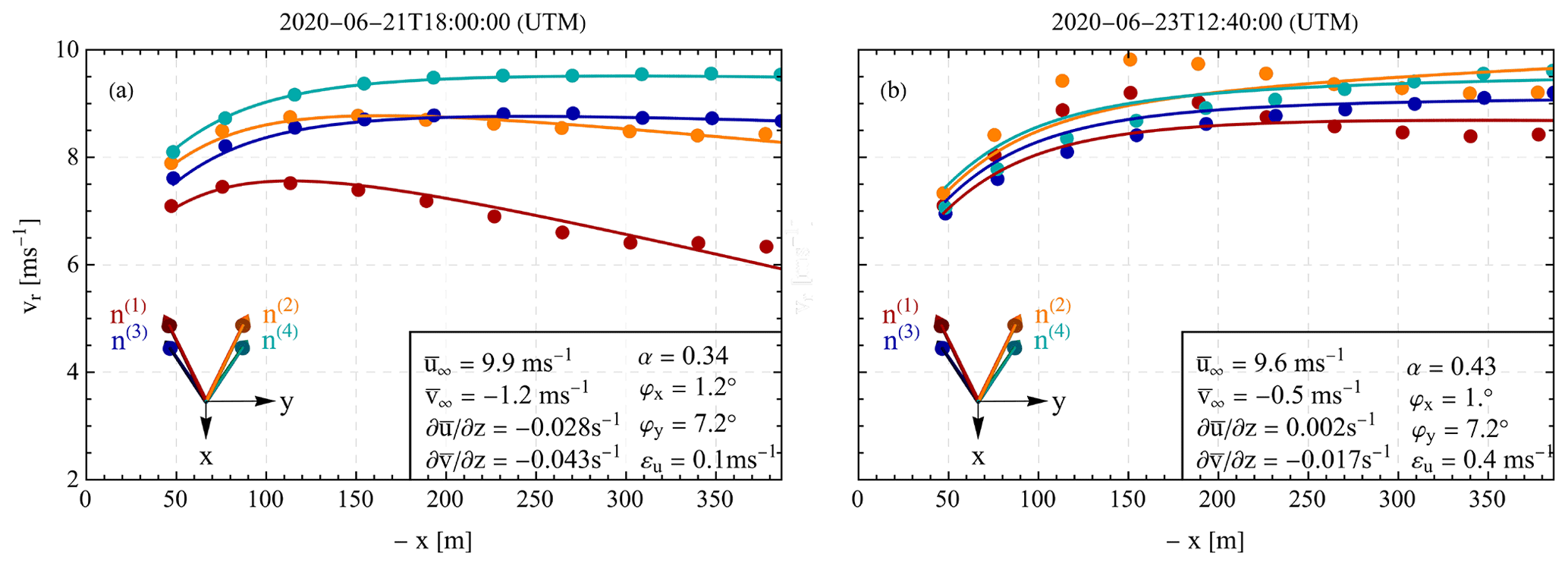
Figure 4Example of two 10 min periods where Eq. (5) either adequately (a) or inadequately (b) describes the measured radial wind speed per upwind distance. The dots correspond to the mean radial wind speed measured by the Wind Iris, and the solid lines represent the corresponding simulated radial wind speeds of each of the four line of sights for the upwind distances between 50 and 400 m, using the fitted parameters presented in the bottom-right part of each plot. The negative x axis denotes upwind distances in accordance with the coordinate system shown in Fig. 3.
We assume using Eq. (9) that the transverse profile of the flow in the wake can be described by a wind speed deficit with a Gaussian distribution. A similar wake model is presented in Aitken et al. (2014) and applied to nacelle-mounted wind lidar data in Aitken and Lundquist (2014). The parameterization of the radial speed measurements in the wake using Eq. (9) enables the investigation of not only the propagation of the wake center due to wake meandering, but also the impact of potential wind direction changes in the area scanned by the wind lidar. This is possible since each of the two aforementioned parameters induces a different pattern in the distribution of the radial wind speeds along the transverse axis. Similar to the analysis of the upwind conditions, the solution of Eq. (9) was computed using a non-linear model solver in Mathematica (Wolfram Research), based on the 30 min mean values of the radial speeds. The solver was applied in each streamwise distance, and the measurements at were chosen as an input of the initial estimation of the free wind and wake parameters. This choice is supported by the sufficient number of measurements distributed in the transverse direction and a well-defined wake profile (an example is presented in Fig. 9c).
4.1 Free wind
During the approximately 3.5-month period when the Wind Iris was operating, a total of 10 529 10 min periods of data were acquired, corresponding to a 70 % system availability. Equation (8), which describes the measured radial wind speeds as a function of the mean upwind conditions, was applied to 4502 10 min periods. They were selected on the basis that (i) both Wind Iris and SCADA data were available (9348), (ii) the wind turbine was operating (7900), (iii) radial wind speed measurements were available in all 10 ranges (7315), and (iv) the yaw direction was between either 90 and 270∘ or 12.5 and 37.5∘ (4502) to avoid cases where the Wind Iris measured partially or fully in the wake of one of the adjacent wind turbines. We selected those wind directions based on the wind farm layout (see Fig. 1b) and by investigating the standard deviation of the line-of-sight measurements of the two lower beams of the upwind-staring lidar. In those wind direction sectors, we observed consistent values of the standard deviation of the radial speeds. This finding is typical in free wind conditions, as shown by Held and Mann (2019).
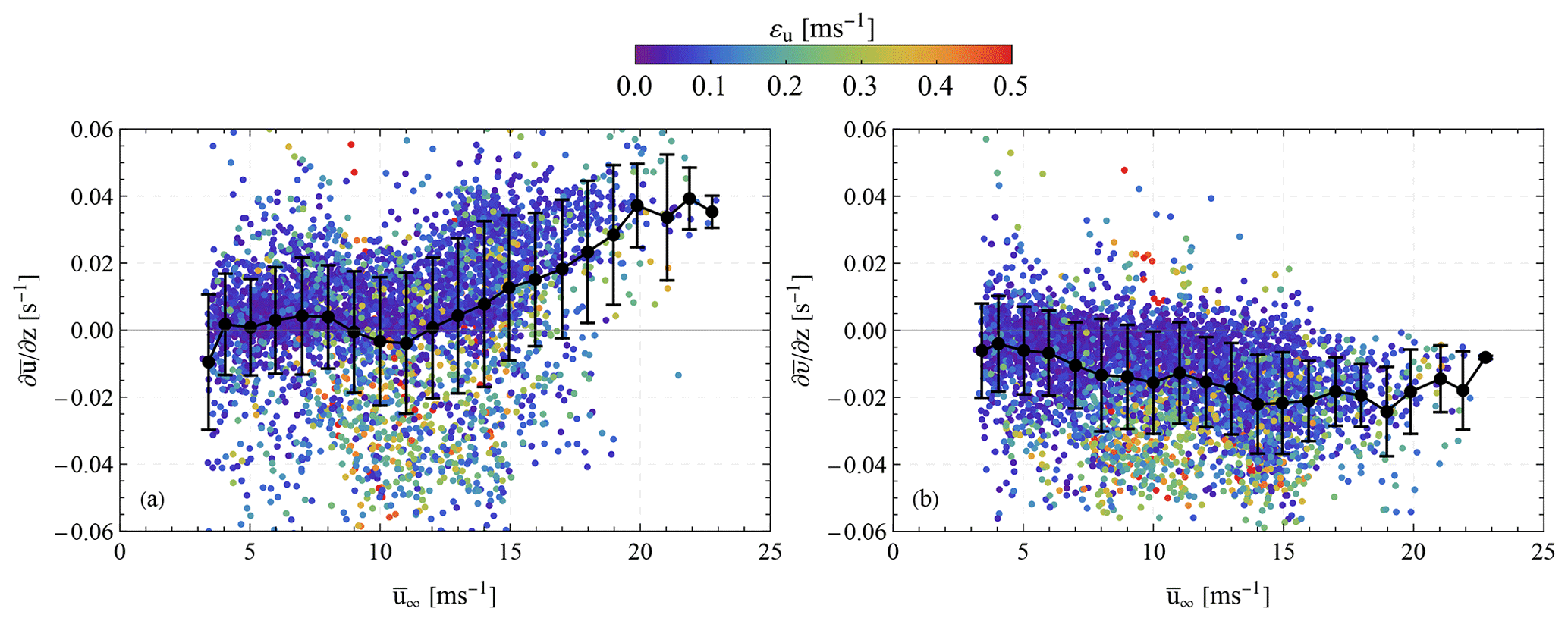
Figure 5Scatterplot of the 10 min mean wind sheer (a) and veer (b) versus the longitudinal component of the mean free wind speed. The color scale depicts the magnitude of the root mean square error εu of the fit of the 10 min mean radial wind speed measurements of the Wind Iris to Eq. (8). The mean and standard deviation sheer and veer in different 1 m s−1 bins are presented with blacks dots and error bars, respectively.
Figure 4 presents two samples of 10 min mean radial wind speed measurements of each of the four line-of-sight beams (denoted in the figure as n(1) and n(2) for the two top beams and n(3) and n(4) for the two bottom beams, shown as arrows), along with the simulated radial wind speeds using the estimated values of the upwind conditions and Eq. (8). The figure presents two cases where the applied model is found to describe either accurately (Fig. 4a) or inaccurately the wind conditions (Fig. 4b), determined by relatively low or high values of εu, respectively. In both plots, we observe that the radial speed values of all beams decrease as wind approaches the wind turbine rotor. This is attributed to the induction of the operating wind turbine. However, in Fig. 4a, we see that the radial wind speeds of the two top beams are lower than those of the corresponding bottom beams and have a decreasing trend as the upwind distance increases. This pattern corresponds to a negative wind shear as it is predicted by the model in this case, where is found to be equal to −0.028 s−1. The reason why the two right beams (n(2) and n(4)) report higher values than the left ones (n(1) and n(3)) is attributed to the negative value of the mean transverse component of the free wind . On the other hand, in Fig. 4b, even though we see a similar trend in the two bottom beams with decreasing speed closer to the rotor, the two top beams present an increase in radial wind speeds with upwind distance up to 180 m, followed by a decrease. The derived wind characteristics in both cases could be attributed to a wind speed profile with an inversion. Such wind profiles are typically observed either in very stable atmospheric stability conditions with a low atmospheric boundary layer height or in the case of low-level jets. Low-level jets are not uncommon over offshore areas in northern Europe. They are characterized by a non-linear wind shear (Emeis, 2014; Kalverla et al., 2019), which in our case results in a high root mean square error εu.
To further investigate the relationship between the fitted values of the wind shear and veer and the resulting root mean square error, we plot the fitted values of and as a function of the mean horizontal wind speed in Fig. 5. Each dot corresponds to a 10 min period, and the color highlights the corresponding value of εu. We observe that on average the wind shear is usually within 0–0.02 s−1, which can be considered to be a low range of values, typical of offshore conditions. However, an increasing trend of the wind shear values is found when the mean free wind speed is higher than 12 m s−1, as seen by the mean shear values (black dots) in Fig. 5a. Furthermore, when εu is usually higher than 0.2 m s−1 then negative wind shear cases are found. This is observed in 31 % of the 10 min periods examined. This shows that wind profile inversions are common at those heights (100–150 m) and should be considered when studying the wind turbine operation. In the case of , we find generally negative values that on average range between 0 to −0.2 s−1 (Fig. 5b). These values are expected from the Ekman spiral in the Northern Hemisphere. Similarly to the wind shear, high εu is related to strong negative values of .
For assessing the accuracy of the model of Eq. (8), we compare the 10 min mean horizontal wind speed at hub height with the corresponding values of the nacelle-mounted anemometer. Figure 6a presents a scatterplot between the estimated free wind at hub height based on the Wind Iris and the nacelle anemometer data. For this purpose we use only cases where εu<0.2 m s−1. We find an overall good agreement between the two data sets, with a bias of less than 0.1 m s−1 and a high Pearson correlation coefficient r>0.99. When studying the mean differences between the two data sets we find that the higher errors are observed between 7–9 m s−1 and between 18–22 m s−1, as it is presented in Fig. 6b. This error could be attributed to a non-optimal transfer function used in the nacelle-mounted anemometer.
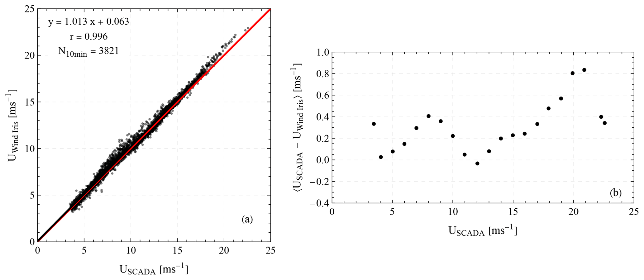
Figure 6(a) Scatterplots of the estimated free wind speed UWind Iris at hub height using the Wind Iris measurements and the corresponding 10 min mean value USCADA as measured by the nacelle-mounted anemometer. (b) Bin-averaged mean difference 〈USCADA−UWind Iris〉 as a function of USCADA.
Furthermore, the Wind Iris data were used to estimate the turbulence intensity (TI) of the ambient wind conditions. The turbulence statistics are not expected to be biased by the wind turbine operation, as it was demonstrated by Mann et al. (2018), where they have showed the induction zone mainly influences the low-frequency fluctuations. Therefore, the measurements acquired the closest to the rotor distance (i.e. 50 m) were used for the estimation of TI. This choice was based on (i) having the smallest spatial separation of the two measuring points that can introduce a bias in the estimated second-order statistics (i.e. standard deviation of u) and (ii) the fact that the vertical displacement between the two line of sights due to the roll angle was on average small, since a 1∘ mean roll angle induced a mean vertical displacement of less than half a meter. Furthermore, at those range gates, we observe the maximum data availability. The estimation was performed by using the 0.25 Hz time series of the radial wind speeds, by solving the equation . In the calculation of the standard deviation of u we do not take into account the contribution of the nacelle's motion to the radial speed. Thus, the estimated TI values are expected to be slightly biased, as it is presented in the work of Gräfe et al. (2022). However, considering the magnitude of the pitch of the wind turbine's nacelle, this error is expected to be less than 15 %.
4.2 Induction zone
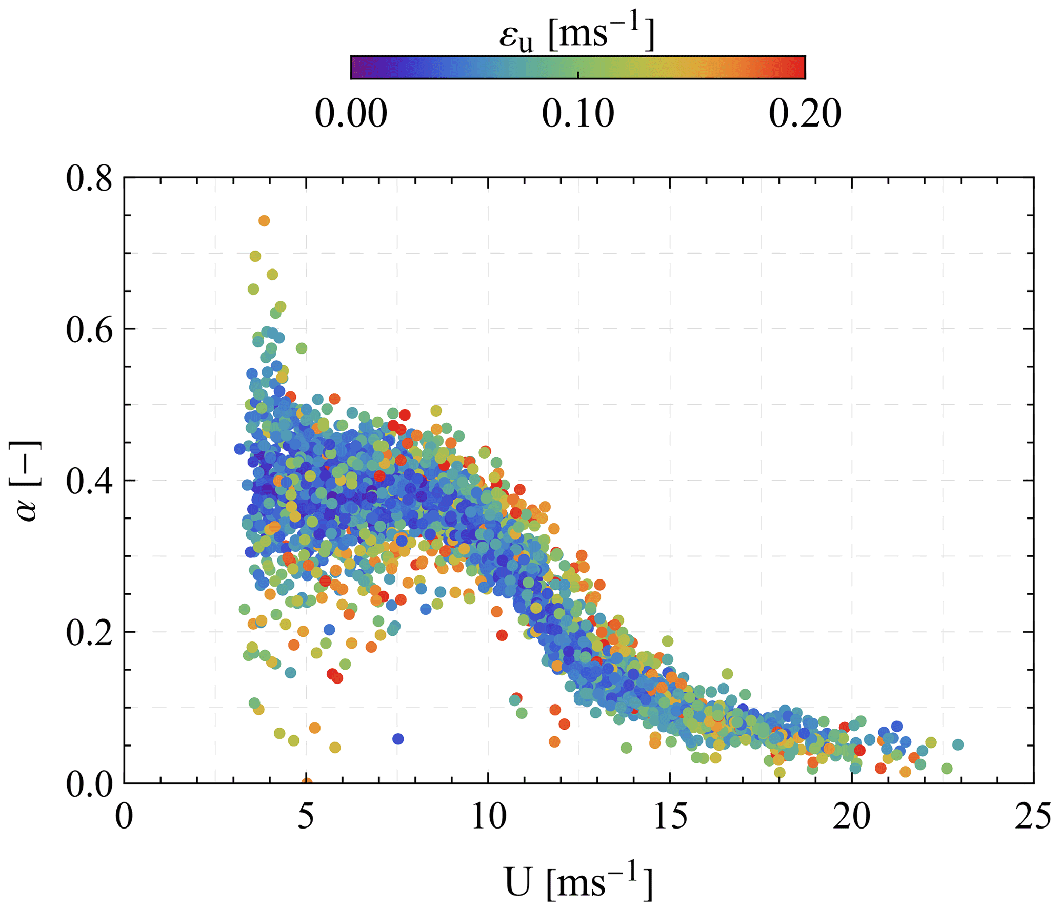
In Fig. 7, the induction factor a is presented as a function of the estimated free horizontal wind at the height of the Wind Iris. Similarly to Fig. 5, the color of each dot denotes the corresponding RMSE εu value of Eq. (8). An increase in the εu results in a spread of the estimated induction factor values per wind speed. In general, we observe that the induction factor is on average equal to 0.37±0.07 in the below rated wind speed range, between 4 and 10 m s−1. These values are close to the theoretical Betz limit, assuming that the operation of a wind turbine can be simulated using an actuator disk model (Hansen, 2015, Chap. 4). Above that wind speed range, the induction factor is decreased until it reaches 0.05±0.02 when the wind speed exceeds 18 m s−1. Overall, we do not observe any correlation between the induction factor and the estimated wind speed shear or veer (plots not shown).
4.3 Wake
In addition to the selection criteria listed in Sect. 4.1 for the characterization of the upwind flow, four additional criteria were included for the wake study. First, only G4000 Galion wind lidar data acquired during periods when the mean tilt angle of the wind turbine was within 4.425 and 5.575∘ were selected, to ensure that the PPI scan was approximately horizontal. This tilt angle range results in a vertical displacement of the furthest range gate by , equivalent to half the dimension of one grid cell. Further, to avoid systematic biases introduced by spatial variations in the data availability, only the scans with a data availability of 75 % or higher were selected. A total of 5907 scanning pattern iterations remained after applying the two criteria above. Subsequently, to study the wake characteristics in relation to the upwind conditions, we first had to identify the 10 min periods where (i) both SCADA and Wind Iris data were available (1719), (ii) the wind turbine was operating (1719), (iii) the inflow was free from wakes (1121), and (iv) the measured radial wind speeds of the Wind Iris could be modeled using Eq. (8) with relatively low errors defined by an empirical threshold of εu<0.2 m s−1 (868).
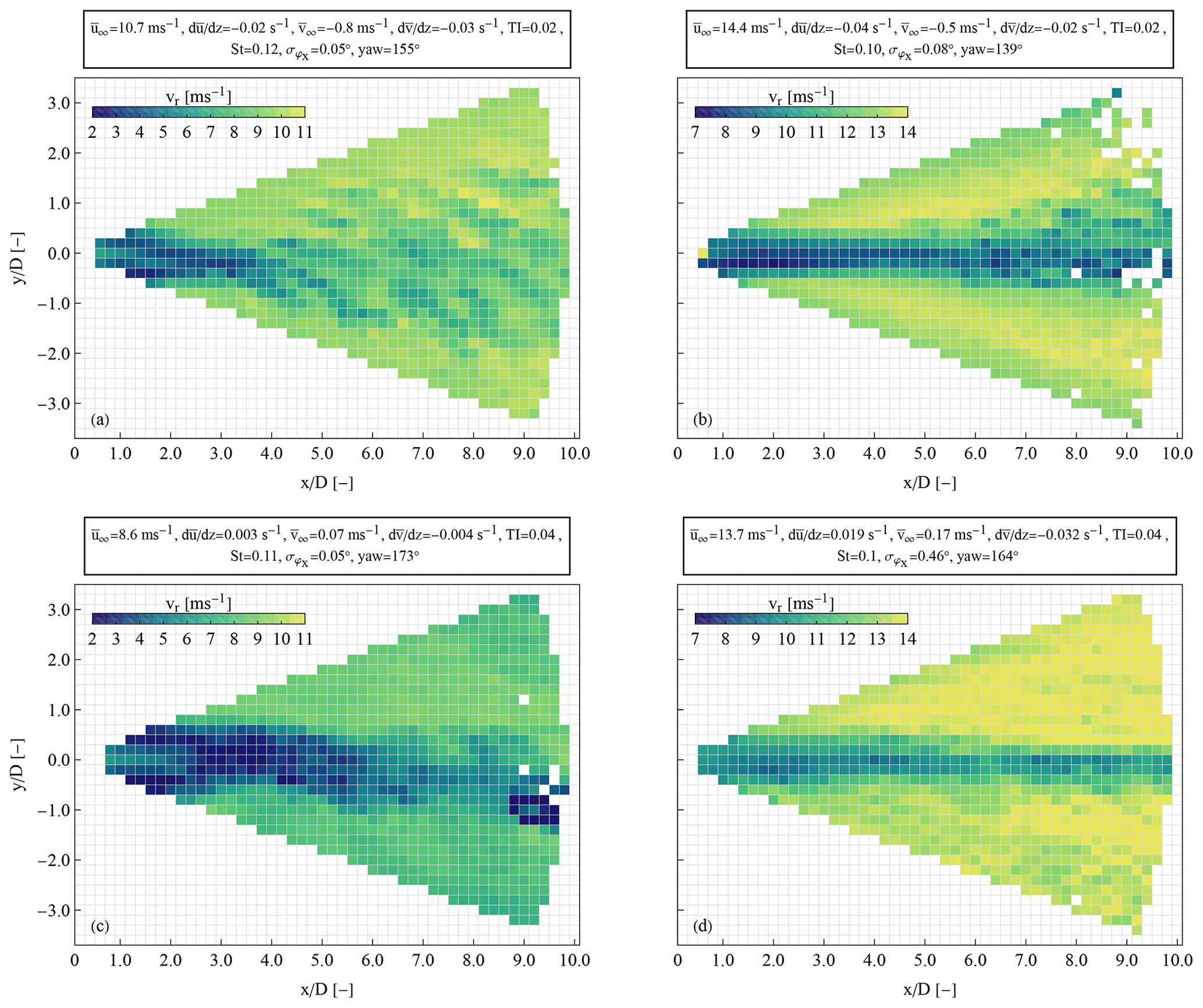
Figure 8Four examples of radial wind speed measurements in the wake flow acquired during individual PPI scans over a 2 min period. The examples correspond to cases with two different levels of turbulence intensity of ∼2 % (a, b) and ∼4 % (c, d), for mean wind speeds below (a, c) and above (b, d) rated speed. The boxes above each plot list the upwind conditions, as well as the Strouhal number (St) of the side-to-side motion, the standard deviation of the roll angle (), and the yaw direction of the wind turbine.
In the wake analysis, and in addition to the parameters of the upwind conditions, we used the variations in the pitch angle to estimate the standard deviation of the velocity of the rotor and the frequency fx of the periodic side-to-side motion to estimate the Strouhal number St for each of the selected cases as . We find that the standard deviation of the longitudinal velocity of the rotor is, on average, 6 times smaller than the standard deviation of the wind speed. Therefore, we can assume that in this field study, the impact of the longitudinal motion of the wind turbine's rotor on the wake conditions is negligible compared to the effect of the random variations in the longitudinal wind speed. Thus, we investigated the wake characteristics as a function of the mean wind speed and turbulence intensity values.
4.3.1 Single wake scan
Figure 8 presents four examples of single wake scans acquired over different 2 min periods. The examples correspond to cases with below and above rated mean wind speeds and two TI levels equal to 2 % and 4 %. The different TI levels could be attributed to the atmospheric stability conditions and possibly to the sea state. We observe that regardless of the turbulence intensity in the above rated speed (Fig. 8b and d), the trace of the wake is visible down to 9 D, without a clear wake expansion. In the case when TI is equal to 2 % (Fig. 8b), we observe a very low standard deviation of the roll angle (∘). Jacobsen and Godvik (2021) studied the response of the wind turbines at Hywind Scotland and found that very low standard deviations of the roll angle were usually associated with stable atmospheric stratification. In Fig. 8b, the wind shear appears to be negative, concordant with a very stable atmosphere, which could explain the propagation of the wake down to 9 D. However, we observe that the wake deficit is still visible but less strong when both the TI and the wind shear increase, as seen in Fig. 8d. This indicates that the different signs of the wind shear do not have a significant impact on the wake propagation, at least for the ambient conditions of the cases examined here.
When the wind was below the rotor rated speed, the 2 min scans showed less systematic characteristics. In the top-left plot (Fig. 8a), we present a case with a negative shear and low standard deviation of the roll angle, indicating a stable atmospheric stratification. The wake deficit is visible down to 4 D, while a reduced wind speed deficit in the range between 1 and 2 D downstream of the nacelle is observed. However, after 4 D, the wake is less evident. Instead, we observe wavy patterns in the distribution of the radial speeds that are spread in the longitudinal and transverse directions. This feature could be attributed to a combination of the flow characteristics (i.e. atmospheric stability and/or wind direction changes) and the relative slow scanning speed of the wind lidar. The PPI scan starts from the positive y axis and rotates towards the negative, possibly explaining the direction of the “stripes” in the plot. This feature is not a necessary characteristic of all the below rated wind speed cases, as shown in the bottom-left plot (Fig. 8c), where the wake trace reaches 9 D and meandering is visible. In Fig. 8c we can also see the effect of the induction zone of one of the adjacent wind turbines (i.e. HS2), when x∼9 D and D.
4.3.2 Mean wake scan
In order to perform a systematic study of the wake characteristics, the individual single scans that were acquired during periods that satisfied the criteria stated in Sect. 4.3 were gathered in 30 min periods and averaged to produce 170 cases of a time-averaged wake in a fixed frame of reference. Furthermore, in the analysis, we chose only periods characterized by a quasi-stationary time series of the longitudinal wind speed, based on the assumption that the time series are quasi-stationary when their dependence on time has a slope of less than 0.5 m s−1 h−1. These periods were identified by applying a linear regression on the 0.25 Hz time series of the longitudinal component measurements from the upwind wind lidar, over different 1 h periods. Finally, we selected only the 30 min periods that had at least 7 PPI scans, which resulted in 89 cases, in which the mean free wind speed was between 8.2 and 14.8 m s−1 and the TI varied between 1.4 % and 8.1 %. For those cases, we found that the fluctuations in the tilt angle of the wind turbine were either correlated or anti-correlated to the time series of the longitudinal wind speed depending on whether the mean wind speed was below or above rated speed (i.e. 10 m s−1), respectively. The mean peak-to-peak difference in the tilt angle for the selected cases equals . On the contrary, the roll angle of the nacelle was characterized by a stronger periodic sinusoidal motion with a varying phase and a mean peak-to-peak difference equal to (see also the power spectral densities presented in Fig. B1). This side-to-side motion corresponds to a mean lateral displacement of the rotor equal to approximately 98.5 m × m or less than 1 % D. The small variations in both the pitch and the roll angle show that the wind turbine is relatively stable regardless of the wind conditions, in accordance with the findings reported by Jacobsen and Godvik (2021), where neither the mean wind speed nor the atmospheric stability had a significant impact on the wind turbine response.
In Fig. 9, we present the mean and the standard deviation, over a 30 min period between 12:30–13:00 LT on 1 September 2020, of the radial wind speeds in the downwind side of the wind turbine. By averaging all scans of the period, we minimize the effect of both random noise and biases due to the natural fluctuations in the wind speed and direction during a single scan (e.g. Fig. 8a). Furthermore, we should expect that the time-averaged wake has a smaller deficit and wider distribution than an instantaneous snapshot of the wake flow. The measured plane covers the downwind propagation of the wake, where wind speed deficits can be traced down to 1500 m (9.7 D). The wake is concentrated within an area with approximately the same width as the wind turbine rotor.
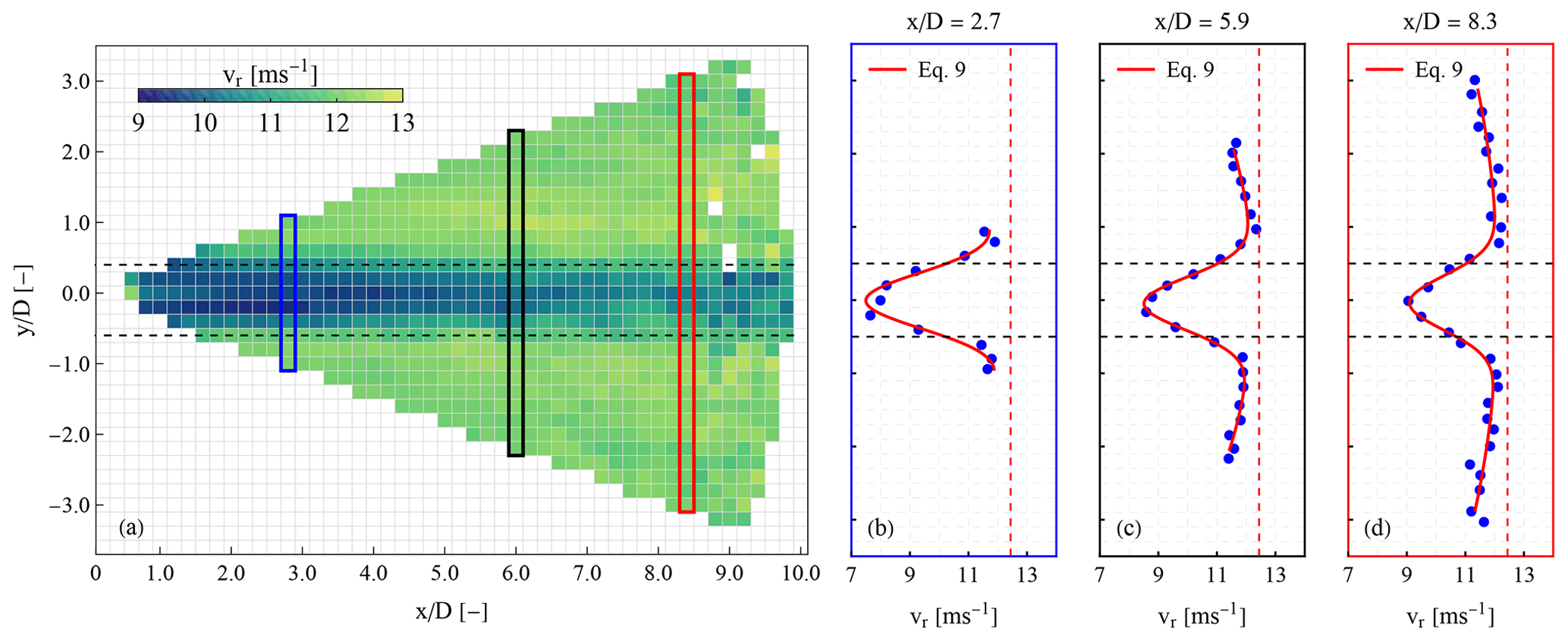
Figure 9(a) Mean radial speeds of a 30 min period over the scanned area and three examples of the transverse profile of the mean and the radial speed (b–d) at , 5.9, and 8.3. The result of the application of Eq. (9) is presented in red in plot (b)–(d).
An example of the application of the wake model of Eq. (9) is presented in Fig. 9b–d for three different downwind distances. Applying a Gaussian model to fit the wake deficit is not always suitable for describing the characteristics of the flow. We assess the model's suitability by investigating the root mean square error εd values between the model described in Eq. (9) and the radial speed profile per downwind distance for each of the 89 cases selected for this study. In Fig. 10, we present the mean values of εd per downwind distance, based on all the selected cases. At close distances, εd takes values above 0.4 m s−1 but decreases with distance. This trend is attributed to the fact that at short distances the measurements are distributed over a limited transverse range of the PPI scan and that the profile of the wake cannot typically be described by a single Gaussian deficit (e.g. Aitken et al., 2014). We empirically define the acceptable threshold of valid application of the model as εd<0.25 m s−1. Using this criterion, we conclude that the adequate model area is within the range . The increase in εd, at the range , is attributed to both the lower SNR of the measurements at those distances, which typically results in higher random errors in the measured radial speeds, and the fact that occasionally the flow in those ranges was further distorted by the induction zone of the adjacent wind turbines.
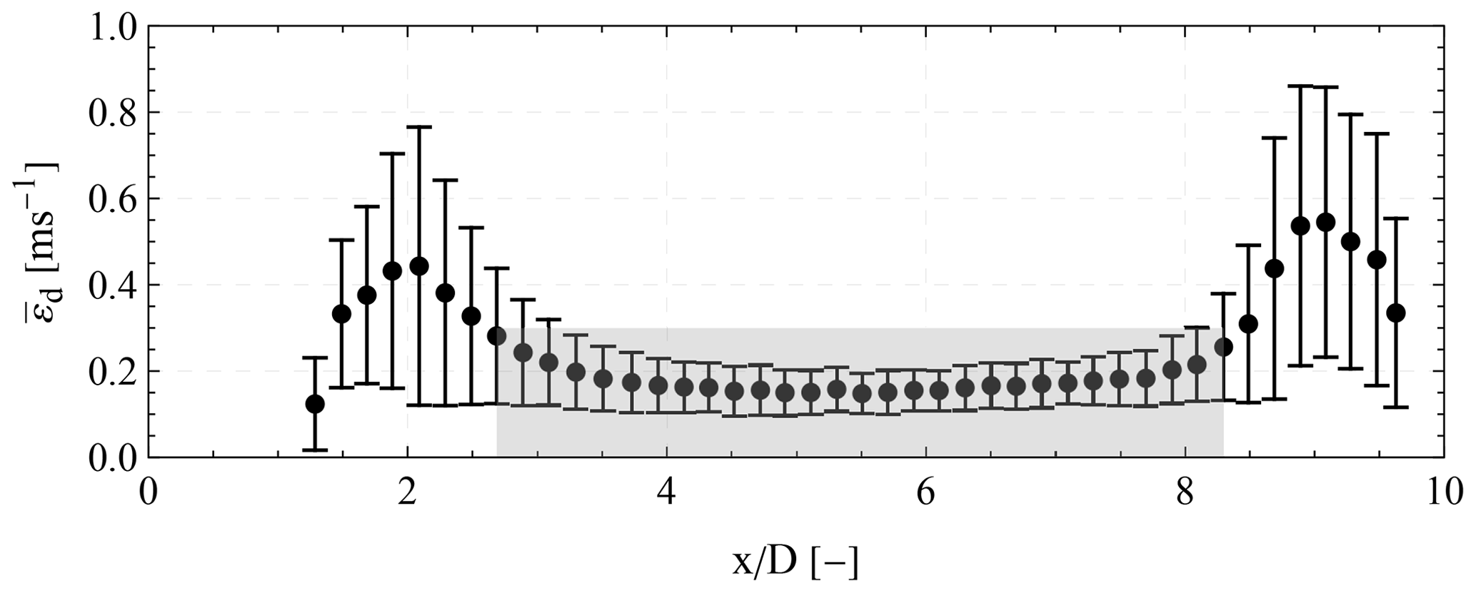
Figure 10The mean (black dots) and standard deviation (error bars) of the root mean square error εd between the acquired radial wind speeds and the Gaussian wake deficit of Eq. (9) for different downwind distances. The opaque gray rectangular area denotes the limits over which, on average, we observe acceptable εd values and thus denotes the range over which the velocity deficit in the wake can be simulated reasonably well by a Gaussian distribution.
To investigate the accuracy of Eq. (9), we assumed that the free wind speed is constant along the whole measured area where wakes are absent. Then, the ensemble average of the free wind speed is calculated based on the mean of the free horizontal wind values, U, estimated in each downwind distance between 2.7 and 8.3 D. Subsequently, the estimations are compared to the ones derived using the Wind Iris data. Using a regression analysis, based on the least-squares perpendicular distance method (Deming fit), we find that the down- and upstream estimations of the horizontal wind speed have a good correlation (i.e. r=0.99) and a small bias ( m s−1). We also find good agreement in the estimated mean yaw misalignment γ. In particular, based on the upwind-staring nacelle lidar (i.e. Wind Iris), the mean γ over the 89 examined 30 min periods is equal to , while from the downwind scanning lidar it is .
4.3.3 Self-similarity in the far wake
To investigate the similarity in the far wake, we calculate the self-similar velocity defect f as a function of the scaled cross-stream variable ξ, which, according to Pope (2000, Chap. 5), are defined as
where and σ correspond to the half width of the half maximum of the wind speed deficit and the standard deviation of the Gaussian distribution of the wind deficit, is the mean free wind speed, is the mean longitudinal wind speed, and y0 is the center of the wake. For estimating the values in the wake, we first assume that the mean vertical speed component is zero. This assumption is based on both the offshore wind conditions and the fact that the flow in the far-wake region of the wake is mainly related to the ambient wind conditions (Vermeer et al., 2003). Thus, one should not expect any rotational motion in the wake flow after , as seen in Zhang et al. (2012), which would introduce a vertical component in the wind vector. Therefore a mean radial wind speed measurement at a given point {x, y} is equal to the projection of the mean and components to the line-of-sight direction:
where γ and ϕ, similarly to Eq. (9), denote the yaw misalignment and the azimuth direction of a line of sight, respectively.
Since the ϕ angles are small {−20, 20∘}, and the mean absolute yaw misalignment, derived from the estimated values of and of the 89 selected periods, is equal to , we can neglect the term without introducing a bias. Thus, through Eq. (11) we can express the mean component as
Therefore, the longitudinal wind speed at the center of the wake y0, using Eqs. (9) and (12), is equal to
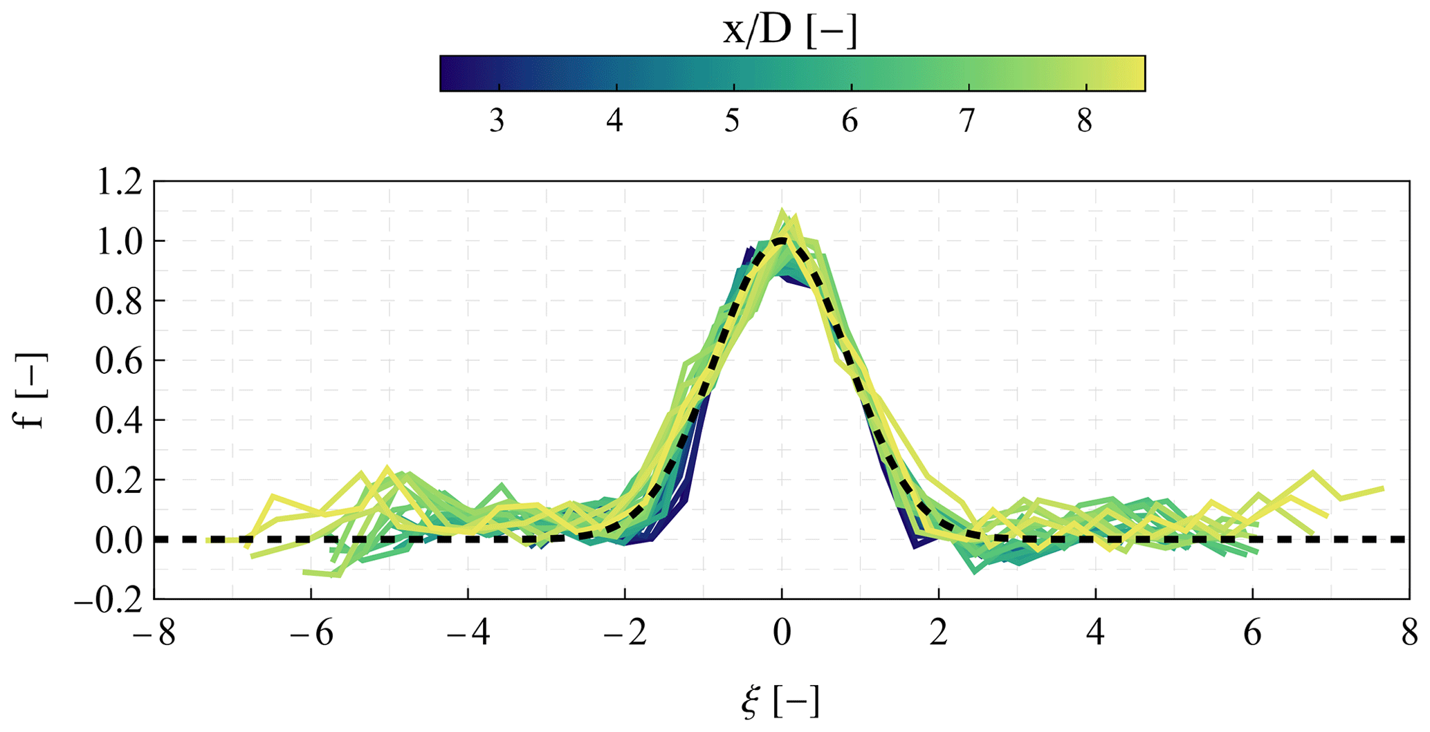
Figure 11Mean profile over a 30 min period of the self-similar velocity defect f as a function of the scaled cross-stream variable ξ for different downwind distances between . The dashed line corresponds to the theoretical distribution .
An example of using Eqs. (12) and (13) in Eq. (10) is presented in Fig. 11 for a 30 min period with a mean free speed equal to 13 m s−1. The figure presents the transverse profile of the self-similar velocity defect for different downwind distances between . We visually observe that the estimated profiles of the velocity defect f are independent of the downwind distance and can be expressed as a function of the variable ξ of Eq. (10). Furthermore, we find that the velocity defect profiles are in good agreement with a Gaussian distribution, defined as . This observation shows that in this case study, a uniform turbulent viscosity could be used to simulate the far-wake flow reasonably well (van der Laan et al., 2023).
Subsequently, we apply the same analysis for all selected 89 30 min periods. Between 3–10 D, we find relatively low RMSE εf values (<0.25 m s−1) between the estimated and modeled velocity deficit profile. This result supports the hypothesis that the profile of the velocity deficit is generally self-similar and, thus, independent of the downwind distance, regardless of the mean free wind speed and the corresponding turbulence intensity. The results here agree with the findings of Chamorro and Porté-Agel (2009), who, in a wind tunnel study, found that the vertical profile of the wind speed deficit in the wake developed over both smooth and rough surfaces is approximately symmetric.
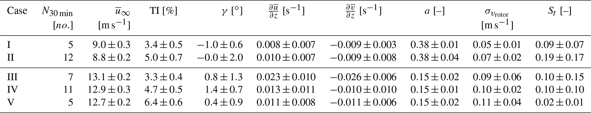
Table 1The number of 30 min periods N30 min and the corresponding characteristics of the upwind profile (longitudinal speed , turbulence intensity TI, yaw misalignment γ, shear and veer , σu) at hub height, the wind turbine's induction zone (a), the standard deviation of the wind rotor speed (), and the Strouhal number of the side-to-side motion (St) for each of the five cases examined.
4.3.4 Case studies
Before studying the wake characteristics for different ambient free wind conditions, we investigate the variability in the wake measurements between 30 min periods with the same mean wind speed and TI values. In Fig. 12, we present 11 profiles of the mean longitudinal wind speed at the center of the wake when the 30 min mean wind speed is equal to 9 m s−1 and TI is equal to 5.0 %. The wind speeds were normalized by dividing them by the mean horizontal wind speed of each 30 min period estimated using Eq. (9). The profiles are generally in agreement in the region . Profile no. 1, where a faster wake recovery (smaller velocity deficit as the downwind distance increases) is observed, is an exception, with no apparent correlation with the wind shear or veer values. Furthermore, in profile nos. 2, 5, 9, and 10, we see a decrease in the radial wind speeds when is between 8.5 and 10. This decrease is attributed to the presence of the induction zone of neighboring wind turbines. Therefore, we apply an additional filter by removing measurements beyond 8.3 D, regardless of the value of εd. Moreover, the 30 min periods with negative shear are also excluded from the analysis in order to avoid cases with inversions in the upwind wind profile.
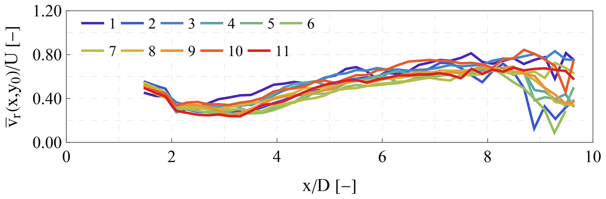
Figure 12Wind profiles of the velocity in the wake center normalized by the mean wind speed for 11 cases when the 30 min mean wind speed was equal to 9 m s−1 and the corresponding TI was equal to 5 %.
After applying the two additional filtering criteria, we examine two cases where the mean wind speed is either below (i.e. 9 m s−1) or above (i.e. 13 m s−1) rated speed. In these two mean wind speed values, we have the maximum number of cases (17 and 23, respectively), which thus enables the estimation of the statistical variability of the derived mean parameters. The data from these cases are split and examined based on their TI values. The wind conditions of these cases and the corresponding upwind profiles are presented in Table 1 and Fig. 13, respectively. We observe that, on average, the wind shear and veer have similar values for all cases. An exception is case III, where stronger shear and veer values are found. Overall, as seen in Fig. 13, we observe that the measured longitudinal and transverse wind components increase linearly with height, which supports our hypothesis of constant shear and veer in Eq. (1). In all cases, the absolute yaw misalignment is less than 2∘, and we find a Strouhal number (St) of the side-to-side motion between 0.1 and 0.2, except for case V where even lower values of St are observed. For each of the selected five cases we study the wake characteristics in terms of the downwind propagation of the wake center's position, the wake's spread, and the maximum velocity deficit.
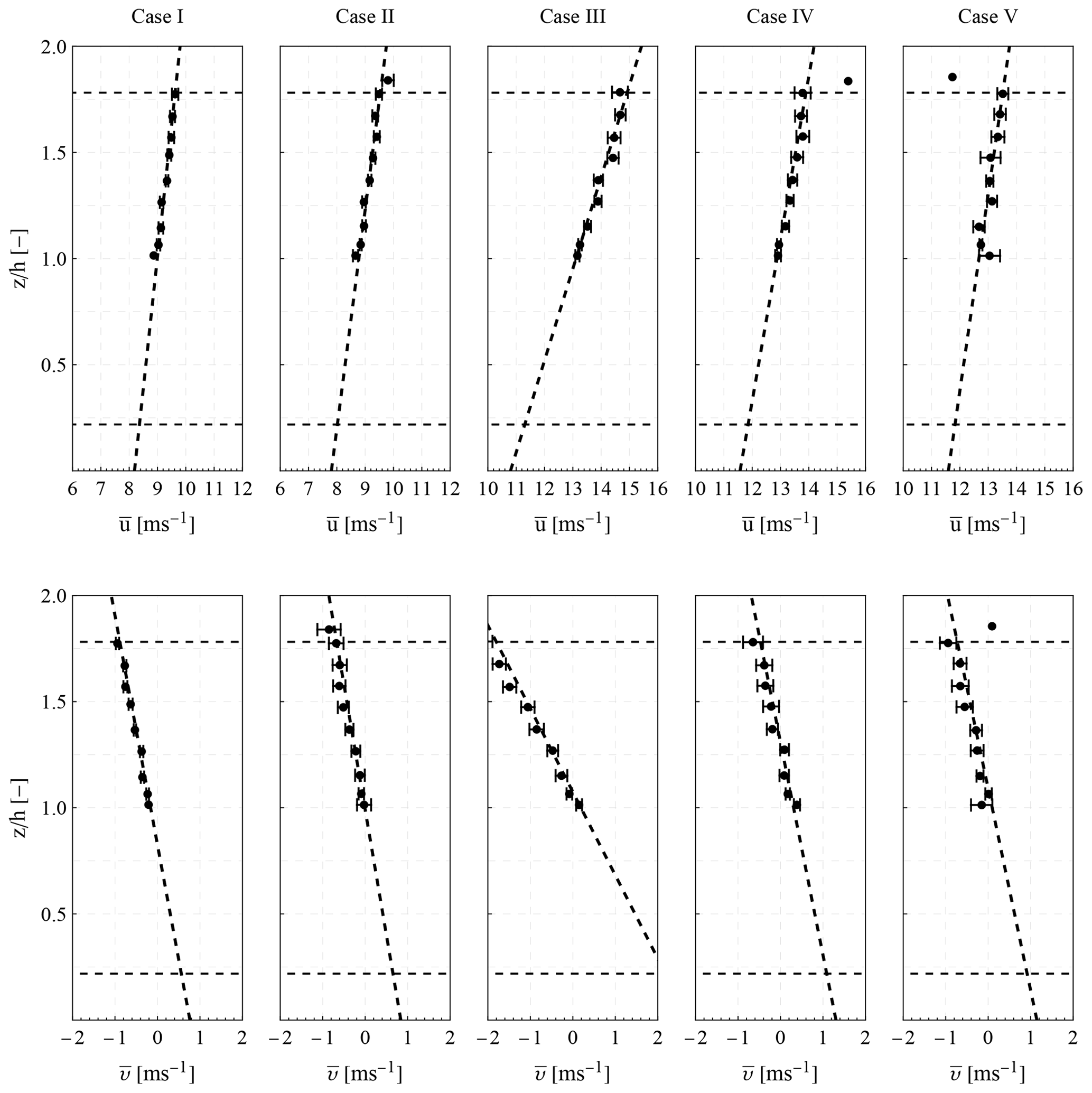
Figure 13Vertical profiles of the mean longitudinal (top row panels) and transverse (bottom row panels) components of the wind vector for each of the five cases (I–V) examined. The measurement height is normalized by hub height h, and the two horizontal dashed lines in each plot denote the lower and upper limits of the wind turbine's rotor. The error bars correspond to the standard error in each estimated mean value.
4.3.5 Wake center
The propagation of the wake center y0, normalized by the rotor diameter D, for each of the five cases is presented in Fig. 14. The y0 values are derived from fitting the radial speed model of Eq. (9) to the measurements of the scanning wind lidar in each downwind distance ranging from 2.6 to 8.3 D. Subsequently, the mean and the standard error of the y0 values for each of the cases examined were calculated. In cases I and II (Fig. 14a), we observe that the wake center is translated towards the negative y axis with an increasing trend with the downwind distance down to approximately 7 D. The observed translation of the wake center could be partially attributed to the estimated yaw misalignment angle γ values presented in Table 1. According to those values the maximum yaw misalignment of the examined cases was equal to −2∘, which could result in a transverse displacement by −0.3 D at 8 D. On the contrary, in cases III–V, even though the estimated yaw misalignment angles are of the same magnitude, the mean wake center, presented in Fig. 14b, shows hardly any translation. Specifically, it is within 0.05 and −0.10 D from the center of the rotor within the downwind range 3–8 D, with, however, larger standard error values (denoted as error bars in Fig. 14). We could not find any correlation between these trends and any other free wind condition characteristics. In all cases, the standard error of the wake center increases with the downwind distance, which could be attributed to the meandering of the wake.
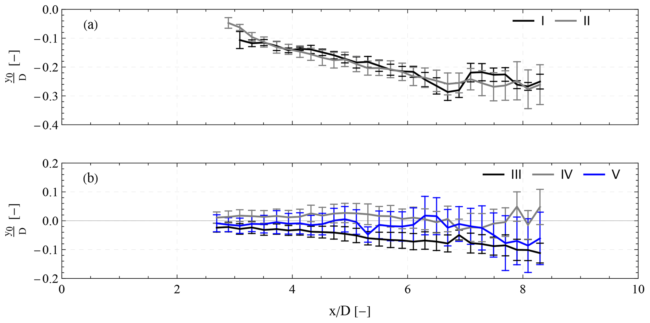
Figure 14Mean wake center along the downwind distance between 2.7 and 8.3 D in a fixed frame of reference when the mean wind speed is equal to (a) 9 m s−1 (below rated speed) and (b) 13 m s−1 for different TI levels that range from 3.4 % to 6.3 % (see Table 1). The error bars correspond to the standard error in each mean value.
4.3.6 Wake width
Similarly to Aitken et al. (2014), we define the wake width equal to 4σ, i.e. the spanwise range where the 95 % wind speed deficit is concentrated. The values are normalized by the rotor diameter D and presented in Fig. 15. In all cases, we observe an increase in the wake width with downwind distance. Below rated (cases I and II in Fig. 15a), already at a downwind distance of 3 D, the wake width is approximately equal to 1.5–2.0 D and increases up to 2 times at 8 D. This wake expansion is similar to the one reported in the case of field studies of onshore wind turbine wakes by Aitken and Lundquist (2014) and Bodini et al. (2017). Furthermore, as the ambient TI increases from 3.4 to 5.0 % the wake width also increases. In the above rated cases in Fig. 15b, we find a slowly growing width as a function of downwind distance, with values ranging between 1.3 and 2.0 D. In these cases (III–V) the observed expansion takes place after 5–6 D. The relatively constant values indicate a slow wake recovery in the 3.3 %–6.4 % TI range.
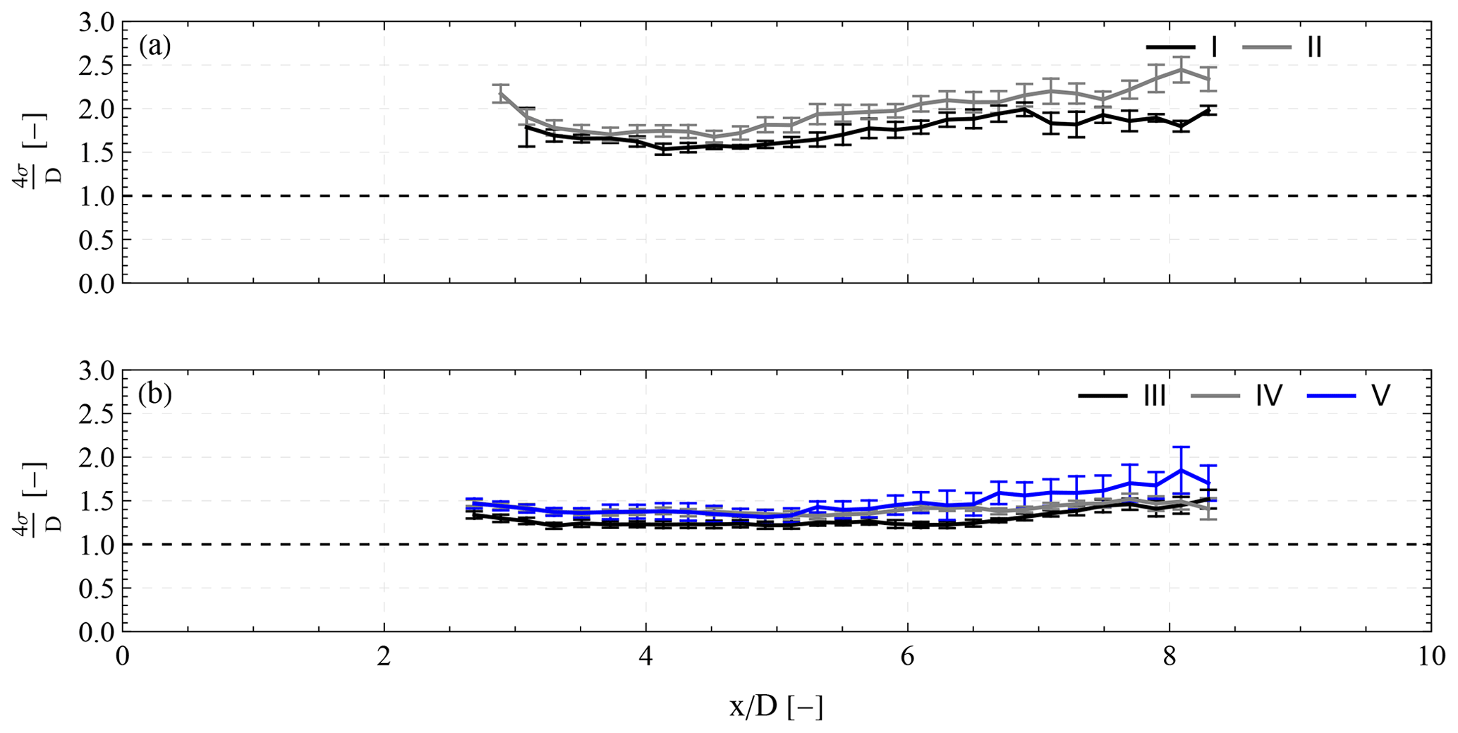
Figure 15Mean wake width along the downwind distance between 2.7 and 8 D in a fixed frame of reference when the mean wind speed is equal to (a) 9 m s−1 (below rated speed) and (b) 13 m s−1 for different TI levels. The error bars correspond to the standard error in each mean value.
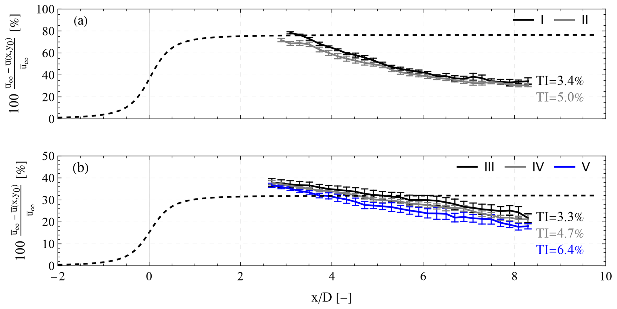
Figure 16Mean velocity deficit at the wake center along the downwind distance between 2.7 and 8.3 D when the mean wind speed is equal to either 9 m s−1 (a) or 13 m s−1 (b) (below rated speed) and for different TI levels. The dashed gray line in each plot represents the predicted longitudinal speed using Eq. (2) and the induction factor values of a=0.38 (a) and a=0.15 (b).
4.3.7 Velocity deficit
The velocity deficit in the center of the wake can be expressed as the relative difference between the mean longitudinal wind component in the center of the wake along the spanwise axis and the free wind speed . Thus, using Eq. (13) and by assuming that , the velocity deficit in the wake center is equal to
where β(x) and σ(x) correspond to the fitted values in Eq. (9). In Fig. 16, we present the percentage of the velocity deficit for different downwind distances extending from 2.7 to 8.3 D, when the mean free wind speed is 9 ms−1 (cases I–II) and 13 ms−1 (cases III–V), respectively. Below rated, in Fig. 16a, we observe a maximum velocity deficit around 69 %–78 % at 3 D that decreases to 38 %–41 % at 8 D. The estimated percentages of the velocity deficit have relatively low standard errors that, depending on the downwind distance, range between 0.7 %–3.1 %. Furthermore, we observe that a 1.6 % increase in TI results in a velocity deficit decrease of 7.5 % ± 3.0 % in the range between 3 and 8 D, which is independent of the downwind distance. The observed high-velocity deficit values at x=3 D agree with the high induction factors presented in Fig. 7. By taking into account the induction factor value and Eq. (2), we should expect a maximum relative velocity deficit, equal to twice the induction factor 2a×100 % = 76 % (which is presented by a dashed black line in Fig. 16a). We therefore find that, especially in case I, the velocity deficit at 3 D is approaching the theoretical maximum relative velocity deficit. However, in the case above rated, in Fig. 16b, we find that the velocity deficit spans from around 37 %–38 % at 3 D and decreases with increasing distance down to 27 %–29 % at 8.3 D. Thus, the observed velocity deficit at 3 D is almost 8 % higher than the theoretical deficit based on the estimated induction factor (a=0.15). Furthermore, an increase in the TI from 3.3 % to 4.7 % and from 4.7 % to 6.4 % results in a decrease in the velocity deficit of 5.7 % ± 3.4 % and 9.9 % ± 3.8 %, respectively. This decrease becomes larger as the downwind distance increases. Overall, the observed decrease in wind speed deficit is a lot slower than cases I and II. Specifically, we find that wind deficit scales with the downwind distance x on the power of −0.4, −0.5, and −0.6 for cases III–V, respectively. The slow flow recovery in cases III–V is consistent with the slow expansion of the wake width that is observed in Fig. 12. These values are lower than in cases I and II where we find that the wind deficit scales with the downwind distance on the power of −0.9, which is in close agreement with the findings of Barthelmie et al. (2004).
To investigate the impact of the ambient atmospheric wind conditions on the wake flow generated by floating wind turbines, we assumed that (i) the wind shear and veer are constant across the wind turbine rotor area; (ii) the wake flow, on overage, propagates horizontally; (iii) turbulence rather than the atmospheric stability plays the dominant role in the wake recovery; and (iv) estimations of turbulence intensity can be derived by combining radial speed measurements acquired at a 50 m upwind distance and a spanwise separation of 26.8 m (0.17 D).
Regarding the first assumption, constant and height-independent wind sheer and veer were used to parameterize the upwind conditions and simulate the radial wind speed measurements of the Wind Iris lidar. In 74 % of the cases, we have found a good agreement between the Wind Iris measurements and the upwind model of Eq. (3). Cases with a non-constant wind sheer and veer can be attributed to low atmospheric boundary layer height or low-level jets. In either case, measurements at higher and lower heights would provide insight into a more comprehensive description of the vertical profile and are recommended in future studies.
Furthermore, since we used only PPI scans in this analysis, it was not possible to study if vertical motions of the wake occurred, which could introduce a bias in the observed velocity deficits. For this reason, we had to hypothesize that the mean wake propagation takes place horizontally. Observations that support this hypothesis have been acquired by the Galion wind lidar on HS2 that was measuring in a RHI scanning mode (see more in Appendix A). The measurements of that lidar could not be analyzed in depth since, due to the layout of the wind farm (see Fig. 1) and for the wind direction sector examined in this study (southern winds), the inflow of HS2 included wake flows from adjacent wind turbines. However, when we investigated the measurements from that lidar for northern wind directions and for the same wind speed ranges (see Fig. A1), we observed that on average we could not detect a significant vertical motion of the center of the wake (see Fig. A2). Overall, assessing the wind characteristics with a scanning lidar is challenging but also offers a lot of possibilities. The acquired data sets point to the direction that wind lidars are technologically mature enough to be used in monitoring the flow around offshore floating wind turbines. As a future best practice, we recommend a combination of PPI and RHI scanning configurations to study the mean characteristics of floating wind turbine wakes. For example this would enable a more thorough study of the features that we observed in the downwind propagation of the wake center (Fig. 14). Furthermore, due to the relative stable response of the floating wind turbine examined in this study, an active motion compensation was not implemented in the scanning wind lidar. However, this could be necessary for the monitoring of the wake flow, especially in the far-wake region, in the case of floating wind turbines that are characterized by larger motions.
A limitation of this study was the lack of information about atmospheric stratification. Unfortunately, during the lidar measuring campaign, no sea surface temperature measurements were available, which could have enabled the characterization of the atmospheric stability. This knowledge would allow a more thorough investigation of the wake properties and their dependence on atmospheric conditions. However, the relatively high speeds, the strong shear values at the examined heights, and the low standard deviation of the roll angles (based on the findings of Jacobsen and Godvik, 2021) support the hypothesis that the data set was acquired during either neutral or stable atmospheric stability, and thus the impact of convective effects of the wake can be considered to be limited.
Finally, regarding the impact of the motion of the floater on the wake characteristics, and considering the measured pitch and roll variations, the amplitude of the surge and sway motions of the wind turbine used in this study was relatively small compared to the values used in numerical (Nanos et al., 2022; Chen et al., 2022) and wind tunnel (Fu et al., 2019; Schliffke et al., 2020) experiments, which focused on the study of the effect of the wind turbine motion on the wake characteristics. Comparing the standard deviation of the surge motion speed with the one of the longitudinal wind speed showed that the standard deviation of the wind was 1 order of magnitude larger. For this reason, we studied the wake characteristics as a function of the mean wind speed and TI values. Similar amplitudes of side-to-side motion with the one observed in our study, with, however, an almost double Strouhal number, have been reported in the work of Li et al. (2022). They state that the side-to-side motion amplifies the wake meandering when the ambient TI is low (<3 %), leading to a faster recovery of the wake deficit. However, in the 4 %–8 % TI regime studied here, the wake recovery of a floating wind turbine is similar to that of a fixed wind turbine, as reported by Li et al. (2022). This similarity in wake recovery could explain the agreement of the wake characteristics presented in this analysis with results from previous numerical and wind tunnel studies of fixed wind turbine wakes. In this study we have not investigated the impact of the rotational speed of the rotor and the blade pitch angles on up- and downwind conditions, which could be a subject of future work.
This study uses two nacelle-mounted wind lidars to investigate the characteristics of the up- and downwind conditions relative to an offshore floating 6 MW wind turbine, which was mounted on a ballast platform. The acquired radial wind speeds from the two lidars are parameterized as a function of the upwind and wake characteristics. In the case of the upwind conditions, we find that, in 74 % of the cases, modeling the radial speeds as a function of a linear wind shear and veer along the rotor, and of an induction factor due to the wind turbine's operation, performed adequately. Over the examined data set, we found that in 31 % of the cases, the wind shear had negative values. These negative values highlight that deviations from a linearly increasing profile at a height range between 100 and 150 m are not negligible in the wind profile at the offshore area of east of Scotland. The wake study focused on the self-similarity of the wind deficit and the downwind propagation of the wake's center, width, and deficit in the far-wake region. The knowledge of these parameters is important since they determine the inflow conditions that the adjacent wind turbines would encounter in a wind farm. The wake measurements were grouped based on the mean wind speed at hub height and the corresponding TI, allowing for a statistical analysis of the wake properties. Our findings support the hypothesis that the spanwise velocity deficit in the wake can be considered self-similar in the far-wake region (3–8 D). Finally, an increase in the ambient TI enhances the recovery of the velocity deficit and the expansion of the wake. These results indicate that the wakes of floating wind turbines, which do not experience high pitch and roll rotations, will have similar characteristics to those of fixed wind turbines. Thus, even though the rotor of the floating wind turbine investigated in this study was subject to motions induced by both wind and sea fluctuations, the primary mechanism for the wake recovery is considered to be the atmospheric turbulence.
The Galion on the HS2 wind turbine scanned in two alternating modes, i.e. a PPI and a range height indicator (RHI) scan. The PPI scan had the same characteristics as the one performed by the Galion lidar on HS4. The RHI scan consisted of 36 line-of-sight measurements with elevation angles that extended from −15 to 20∘. In our study, the RHI measurements acquired on the HS2 wind turbine were used only to investigate the average vertical motion of the wake. Figure A1 presents the mean longitudinal speed, estimated by dividing the radial wind speed measurements by the cosine of the elevation angle of the line of sight. The estimation of the mean is based on two different data sets based on the wind speed range of 7.4–10.5 and 10.6–13.5 m s−1. The two sets had 426 and 266 scans for the first and second wind speed ranges, respectively. The data are grouped based only on the mean wind speed.
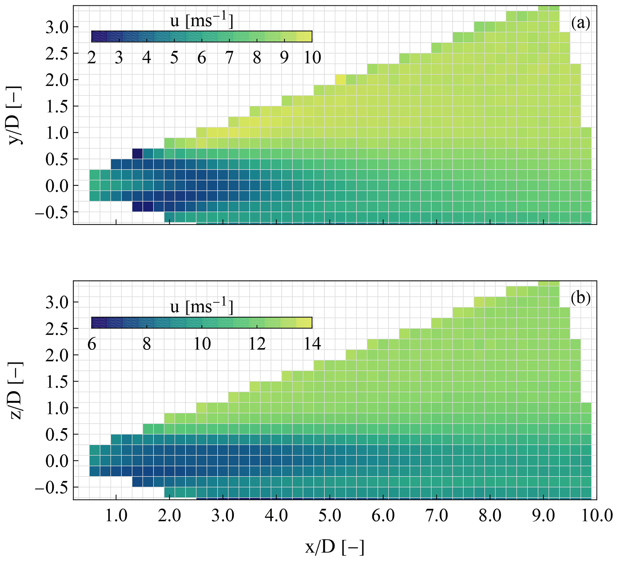
Figure A1Mean longitudinal wind speed acquired during a range height indicator scan for the two different wind speed ranges of (a) 7.4–10.5 m s−1 and (b) 10.6–13.5 m s−1.
Figure A2 presents the vertical profile of the wind speed based on the RHI scans of Fig. A1 for six different downwind distances corresponding to 3, 4, 5, 6, 7, and 8 D. Each profile is normalized by the mean free wind speed at hub height. The profiles show a visible velocity deficit for all the ranges down to 8 D. Furthermore, the maximum velocity deficit is near hub height regardless of the downwind distance. On average, the wake center shows no significant vertical motion even though the pitch angle of the wind turbine's nacelle is 5∘.

Figure A2Vertical profiles of the longitudinal wind speed at different downwind distances (3, 4, 5, 6, 7, and 8 D) and for two wind speed ranges of (a) 7.4–10.5 m s−1 and (b) 10.6–13.5 m s−1.
Figure B1 presents the power spectral density of the pitch (Fig. B1a) and roll (Fig. B1b) angles. We observe that in general higher energy levels appear in the spectrum of the pitch angle, which corresponds to oscillations longitudinal to the yaw direction. However, in the roll angles we observe a more predominant frequency peak at 0.01 and 0.03 Hz, which corresponds to the natural frequency of the sway and roll motions of the wind turbine (Jacobsen and Godvik, 2021), respectively.
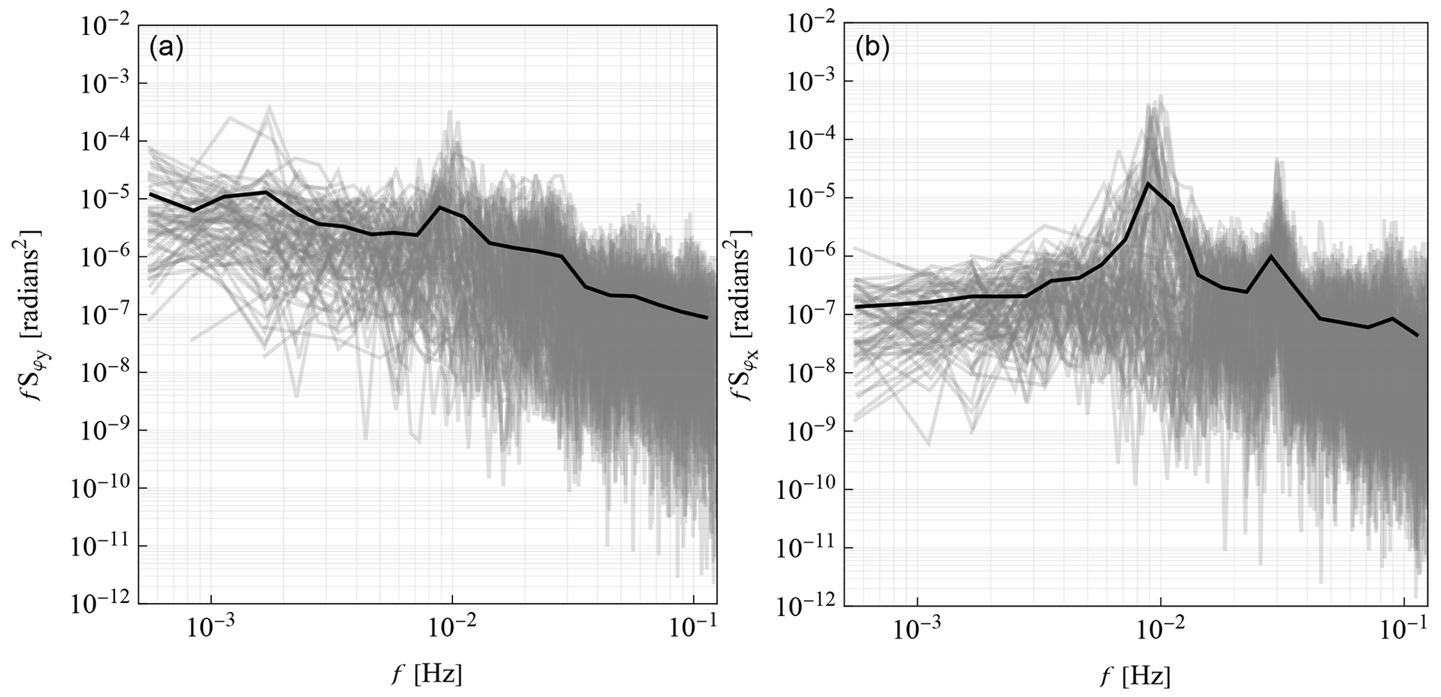
Figure B1Power spectral densities of the pitch (a) and roll (b) angles of the wind turbine measured by a motion reference unit (MRU) in the nacelle. The gray lines correspond to the individual spectra for each of the 89 30 min periods examined in this study, and the black lines depict the corresponding mean over all cases.
The post-processing, filtering, and analysis of the data were performed using the software system Wolfram Mathematica. For more information regarding the code used please contact Nikolas Angelou at nang@dtu.dk.
The data used in this study were acquired by Hywind Scotland. Hywind Scotland gave permission to DTU to analyze the data and publish the corresponding research findings. Due to a confidentiality agreement the data used in this study are not publicly available.
The Hywind Scotland wind farm and CDB planned the campaign and performed the measurements; NA and JM conceptualized the research analysis; NA analyzed the data and prepared the data visualization; NA wrote the original draft of the manuscript; and NA, JM, and CDB reviewed and edited the paper.
At least one of the (co-)authors is a member of the editorial board of Wind Energy Science. The peer-review process was guided by an independent editor, and the authors also have no other competing interests to declare.
Publisher's note: Copernicus Publications remains neutral with regard to jurisdictional claims in published maps and institutional affiliations.
Hywind Scotland is acknowledged for providing access to the data.
This research has been partially supported by the Horizon 2020 project (grant no. 101084205).
This paper was edited by Sandrine Aubrun and reviewed by two anonymous referees.
Aitken, M. L. and Lundquist, J. K.: Utility-Scale Wind Turbine Wake Characterization Using Nacelle-Based Long-Range Scanning Lidar, J. Atmos. Oceanic Tech., 31, 1529–1539, https://doi.org/10.1175/JTECH-D-13-00218.1, 2014. a, b, c
Aitken, M. L., Banta, R. M., Pichugina, Y. L., and Lundquist, J. K.: Quantifying Wind Turbine Wake Characteristics from Scanning Remote Sensor Data, J. Atmos. Ocean. Tech., 31, 765–787, https://doi.org/10.1175/JTECH-D-13-00104.1, 2014. a, b, c, d
Archer, C. L., Wu, S., Vasel-Be-Hagh, A., Brodie, J. F., Delgado, R., Pé, A. S., Oncley, S., and Semmer, S.: The VERTEX field campaign: observations of near-ground effects of wind turbine wakes, J. Turbulence, 20, 64–92, https://doi.org/10.1080/14685248.2019.1572161, 2019. a, b, c
Barthelmie, R., Larsen, G., Pryor, S., Jørgensen, H., Bergström, H., Schlez, W., Rados, K., Lange, B., Vølund, P., Neckelmann, S., Mogensen, S., Schepers, G., Hegberg, T., Folkerts, L., and Magnusson, M.: ENDOW (efficient development of offshore wind farms): modelling wake and boundary layer interactions, Wind Energy, 7, 225–245, https://doi.org/10.1002/we.121, 2004. a
Bingöl, F., Trujillo, J. J., Mann, J., and Larsen, G. C.: Fast wake measurements with LiDAR at Risø test field, IOP Conf. Ser.: Earth Environ. Sci., 1, 012022, https://doi.org/10.1088/1755-1315/1/1/012022, 2008. a, b
Bodini, N., Zardi, D., and Lundquist, J. K.: Three-dimensional structure of wind turbine wakes as measured by scanning lidar, Atmos. Meas. Tech., 10, 2881–2896, https://doi.org/10.5194/amt-10-2881-2017, 2017. a
Borraccino, A., Schlipf, D., Haizmann, F., and Wagner, R.: Wind field reconstruction from nacelle-mounted lidar short-range measurements, Wind Energ. Sci., 2, 269–283, https://doi.org/10.5194/wes-2-269-2017, 2017. a
Brugger, P., Markfort, C., and Porté-Agel, F.: Field measurements of wake meandering at a utility-scale wind turbine with nacelle-mounted Doppler lidars, Wind Energ. Sci., 7, 185–199, https://doi.org/10.5194/wes-7-185-2022, 2022. a, b, c, d
Cañadillas, B., Beckenbauer, M., Trujillo, J. J., Dörenkämper, M., Foreman, R., Neumann, T., and Lampert, A.: Offshore wind farm cluster wakes as observed by long-range-scanning wind lidar measurements and mesoscale modeling, Wind Energ. Sci., 7, 1241–1262, https://doi.org/10.5194/wes-7-1241-2022, 2022. a
Carbajo Fuertes, F., Markfort, C. D., and Porté-Agel, F.: Wind Turbine Wake Characterization with Nacelle-Mounted Wind Lidars for Analytical Wake Model Validation, Remote Sens., 10, 668, https://doi.org/10.3390/rs10050668, 2018. a, b, c, d
Chamorro, L. P. and Porté-Agel, F.: A wind-tunnel investigation of wind-turbine wakes: boundary-layer turbulence effects, Bound.-Lay. Meteorol., 132, 129–149, https://doi.org/10.1007/s10546-009-9380-8, 2009. a, b
Chamorro, L. P. and Porté-Agel, F.: Effects of thermal stability and incoming boundary-layer flow characteristics on wind-turbine wakes: a wind-tunnel study, Bound.-Lay. Meteorol., 136, 515–533, https://doi.org/10.1007/s10546-010-9512-1, 2010. a
Chen, G., Liang, X.-F., and Li, X.-B.: Modelling of wake dynamics and instabilities of a floating horizontal-axis wind turbine under surge motion, Energy, 239, 122110, https://doi.org/10.1016/j.energy.2021.122110, 2022. a, b, c
Conway, J. T.: Analytical solutions for the actuator disk with variable radial distribution of load, J. Fluid Mech., 297, 327–355, https://doi.org/10.1017/S0022112095003120, 1995. a, b
Emeis, S.: Wind speed and shear associated with low-level jets over Northern Germany, Meteorol. Z., 23, 295–304, https://doi.org/10.1127/0941-2948/2014/0551, 2014. a
Fu, S., Jin, Y., Zheng, Y., and Chamorro, L. P.: Wake and power fluctuations of a model wind turbine subjected to pitch and roll oscillations, Appl. Energy, 253, 113605, https://doi.org/10.1016/j.apenergy.2019.113605, 2019. a, b, c, d
Gräfe, M., Pettas, V., and Cheng, P. W.: Wind field reconstruction using nacelle based lidar measurements for floating wind turbines, J. Phys.: Conf. Ser., 2265, 042022, https://doi.org/10.1088/1742-6596/2265/4/042022, 2022. a
Gryning, S. E. and Floors, R.: Carrier-to-noise-threshold filtering on off-shore wind lidar measurements, Sensors, 19, 592, https://doi.org/10.3390/s19030592, 2019. a
Hansen, M. O.: Aerodynamics of Wind Turbines, in: 3rd Edn., Routledge, https://doi.org/10.4324/9781315769981, 2015. a
Held, D. P. and Mann, J.: Detection of wakes in the inflow of turbines using nacelle lidars, Wind Energ. Sci., 4, 407–420, https://doi.org/10.5194/wes-4-407-2019, 2019. a
Iungo, G. V. and Porté-Agel, F.: Volumetric Lidar Scanning of Wind Turbine Wakes under Convective and Neutral Atmospheric Stability Regimes, J. Atmos. Ocean. Tech., 31, 2035–2048, https://doi.org/10.1175/JTECH-D-13-00252.1, 2014. a, b
Iungo, G. V., Wu, Y.-T., and Porté-Agel, F.: Field Measurements of Wind Turbine Wakes with Lidars, J. Atmos. Ocean. Tech., 30, 274–287, https://doi.org/10.1175/JTECH-D-12-00051.1, 2013. a, b
Jacobsen, A. and Godvik, M.: Influence of wakes and atmospheric stability on the floater responses of the Hywind Scotland wind turbines, Wind Energy, 24, 149–161, https://doi.org/10.1002/we.2563, 2021. a, b, c, d, e, f
Kalverla, P., Duncan, J., Steeneveld, G.-J., and Holtslag, B.: Low-level jets over the North Sea based on ERA5 and observations: together they do better, Wind Energ. Sci., 4, 193–209, https://doi.org/10.5194/wes-4-193-2019, 2019. a
Kleine, V. G., Franceschini, L., Carmo, B. S., Hanifi, A., and Henningson, D. S.: The stability of wakes of floating wind turbines, Phys. Fluids, 34, 074106, https://doi.org/10.1063/5.0092267, 2022. a, b
Li, Z., Dong, G., and Yang, X.: Onset of wake meandering for a floating offshore wind turbine under side-to-side motion, J. Fluid Mech., 934, A29, https://doi.org/10.1017/jfm.2021.1147, 2022. a, b, c, d
Mann, J., Peña, A., Troldborg, N., and Andersen, S. J.: How does turbulence change approaching a rotor?, Wind Energ. Sci., 3, 293–300, https://doi.org/10.5194/wes-3-293-2018, 2018. a
Medici, D., Ivanell, S., Dahlberg, J.-A., and Alfredsson, P. H.: The upstream flow of a wind turbine: blockage effect, Wind Energy, 14, 691–697, https://doi.org/10.1002/we.451, 2011. a
Menke, R., Vasiljević, N., Wagner, J., Oncley, S. P., and Mann, J.: Multi-lidar wind resource mapping in complex terrain, Wind Energ. Sci., 5, 1059–1073, https://doi.org/10.5194/wes-5-1059-2020, 2020. a, b, c
Nanos, E. M., Bottasso, C. L., Manolas, D. I., and Riziotis, V. A.: Vertical wake deflection for floating wind turbines by differential ballast control, Wind Energ. Sci., 7, 1641–1660, https://doi.org/10.5194/wes-7-1641-2022, 2022. a, b, c
Peña, A., Hasager, C. B., Gryning, S.-E., Courtney, M., Antoniou, I., and Mikkelsen, T.: Offshore wind profiling using light detection and ranging measurements, Wind Energy, 12, 105–124, https://doi.org/10.1002/we.283, 2009. a
Pope, S. B.: Turbulent Flows, Cambridge University Press, https://doi.org/10.1017/CBO9780511840531, 2000. a
Porté-Agel, F., Bastankhah, M., and Shamsoddin, S.: Wind-Turbine and Wind-Farm Flows: A Review, Bound.-Lay. Meteorol., 174, 1–59, https://doi.org/10.1007/s10546-019-00473-0, 2020. a
Rodrigues, S., Teixeira Pinto, R., Soleimanzadeh, M., Bosman, P. A., and Bauer, P.: Wake losses optimization of offshore wind farms with moveable floating wind turbines, Energ. Convers. Manage., 89, 933–941, https://doi.org/10.1016/j.enconman.2014.11.005, 2015. a
Schliffke, B., Aubrun, S., and Conan, B.: Wind Tunnel Study of a “Floating” Wind Turbine’s Wake in an Atmospheric Boundary Layer with Imposed Characteristic Surge Motion, J. Phys.-Conf. Ser., 1618, 062015, https://doi.org/10.1088/1742-6596/1618/6/062015, 2020. a, b, c
Schneemann, J., Theuer, F., Rott, A., Dörenkämper, M., and Kühn, M.: Offshore wind farm global blockage measured with scanning lidar, Wind Energ. Sci., 6, 521–538, https://doi.org/10.5194/wes-6-521-2021, 2021. a
Simley, E., Angelou, N., Mikkelsen, T., Sjöholm, M., Mann, J., and Pao, L.: Characterization of wind velocities in the upstream induction zone of a wind turbine using scanning continuous-wave lidars, J. Renew. Sustain. Energ., 8, 013301, https://doi.org/10.1063/1.4940025, 2016. a
Trabucchi, D., Trujillo, J.-J., and Kühn, M.: Nacelle-based Lidar Measurements for the Calibration of a Wake Model at Different Offshore Operating Conditions, Energ. Proced., 137, 77–88, https://doi.org/10.1016/j.egypro.2017.10.335, 2017. a
Trujillo, J.-J., Bingöl, F., Larsen, G. C., Mann, J., and Kühn, M.: Light detection and ranging measurements of wake dynamics. Part II: two-dimensional scanning, Wind Energy, 14, 61–75, https://doi.org/10.1002/we.402, 2011. a, b
van der Laan, M. P., Baungaard, M., and Kelly, M.: Brief communication: A clarification of wake recovery mechanisms, Wind Energ. Sci., 8, 247–254, https://doi.org/10.5194/wes-8-247-2023, 2023. a
Vermeer, L., Sørensen, J., and Crespo, A.: Wind turbine wake aerodynamics, Prog. Aerosp. Sci., 39, 467–510, https://doi.org/10.1016/S0376-0421(03)00078-2, 2003. a
Wise, A. S. and Bachynski, E. E.: Wake meandering effects on floating wind turbines, Wind Energy, 23, 1266–1285, https://doi.org/10.1002/we.2485, 2020. a
Wiser, R., Rand, J., Seel, J., Beiter, P., Baker, E., Lantz, E., and Gilman, P.: Expert elicitation survey predicts 37 % to 49 % declines in wind energy costs by 2050, Nat. Energy, 6, 555–565, https://doi.org/10.1038/s41560-021-00810-z, 2021. a
Wu, Y.-T. and Porté-Agel, F.: Atmospheric turbulence effects on wind-turbine wakes: An LES study, Energies, 5, 5340–5362, https://doi.org/10.3390/en5125340, 2012. a
Zhang, W., Markfort, C. D., and Porté-Agel, F.: Near-wake flow structure downwind of a wind turbine in a turbulent boundary layer, Exp. Fluids, 52, 1219–1235, https://doi.org/10.1007/s00348-011-1250-8, 2012. a
- Abstract
- Introduction
- Field study
- Methods
- Results
- Discussion
- Conclusions
- Appendix A: Range height indicator lidar scans
- Appendix B: Pitch and roll angles of the wind turbine's nacelle
- Code availability
- Data availability
- Author contributions
- Competing interests
- Disclaimer
- Acknowledgements
- Financial support
- Review statement
- References