the Creative Commons Attribution 4.0 License.
the Creative Commons Attribution 4.0 License.
 | 28 Feb 2023
Optimization of wind farm operation with a noise constraint
Andreas Fischer
Pierre-Elouan Réthoré
Ju Feng
This article presents a method for performing noise-constrained optimization of wind farms by changing the operational modes of the individual wind turbines. The optimization is performed by use of the TopFarm optimization framework and wind farm flow modelling in PyWake as well as two sound propagation models: the ISO 9613-2 model and the parabolic equation model, WindSTAR. The two sound propagation models introduce different levels of complexity to the optimization problem, with the WindSTAR model taking a broader range of parameters, like the acoustic ground impedance, the complex terrain elevation and the flow field from the noise source to the receptor, into account. Wind farm optimization using each of the two sound propagation models is therefore performed in different atmospheric conditions and for different source/receptor setups, and compared through this study in order to evaluate the advantage of using a more complex sound propagation model. The article focuses on wind farms in flat terrain including dwellings at which the noise constraints are applied. By this, the study presents the significant gain in using a higher fidelity sound propagation model like WindSTAR over the simple ISO 9613-2 model in noise-constrained optimization of wind farms. Thus, in certain presented flow cases a power gain of up to ∼53 % is obtained by using WindSTAR to estimate the noise levels.
- Article
(6032 KB) - Full-text XML
- BibTeX
- EndNote


As the demand for onshore wind farms increases, the social acceptance of wind turbines becomes a larger challenge. One of the main factors contributing to neighbour annoyance is the aerodynamic noise from the wind turbine blades. Previous social studies have shown how neighbours to wind farms experience annoyance and sleep disturbances caused by the noise emitted from wind farms (Michaud et al., 2016; Poulsen et al., 2019, 2018). Thus, in order to successfully continue the expansion of onshore wind energy by either constructing new wind farms or by repowering existing ones, methods to ensure a low noise level are needed. Several wind turbine developers introduce multiple operational modes in the turbine design with the aim of switching to a more noise reducing operation by, for example, decreasing the rotational speed of the rotor. However, modifying the rotational speed to reduce the emitted noise causes a curtailed power output of the wind turbine. A method for effectively choosing at which operational mode each of the wind turbines should operate is therefore needed. By performing noise-constrained optimization of wind farm operations, it is possible to maximize the overall power production of a wind farm while still keeping the noise received at each neighbour under a defined limit. This is done by letting each wind turbine in a wind farm individually switch to the optimal discrete operational mode. Previously, noise-constrained optimization has been performed through layout design of onshore wind farms (Tingey and Ning, 2017; Wu et al., 2020; Sorkhabi et al., 2016; Mittal et al., 2017; Cao et al., 2020). Furthermore, optimization of discrete design variables has previously been done through other layout optimization problems (Riva et al., 2020; Feng and Shen, 2017). However, the work in this article presents a novel way of considering the discrete operational modes in noise-constrained optimization. The optimization of the operation of an existing layout can be needed in the case of repowering of a wind farm or in wind farms that are already heavily derated in order to limit the emitted sound. Currently, the ISO 9613-2 sound propagation model (DS, 1997) is extensively used to determine the location and operation of onshore wind turbines. The model is adapted to the regulations of the specific country, by considering varying values, i.e. for the acoustic hardness of the ground. Some examples of regulations in four European countries are summarized by Nieuwenhuizen and Köhl (2015). In addition, each country has specified noise limits that may vary from day to night or from area to area. In Denmark, the ISO 9613-2 model is used such that the “worst case scenario” noise is modelled. The ground type parameter is thus set to zero, representative of a hard, reflecting ground surface. The Danish regulations further set noise limits for the wind speeds U10 m=6 and 8 m s−1 at 10 m height above the ground. In noise sensitive areas the limits are, for example, defined as 37 dB(A) for U10 m=6 m s−1 and 39 dB(A) for U10 m=8 m s−1 (Nieuwenhuizen and Köhl, 2015). The noise limits are thus in general very vaguely defined by only considering the wind speed and the site of interest. This definition naturally originates from the limitations of the ISO 9613-2 model and the uncertainty of the measured wind speed and wind direction at the site. Instead, a higher fidelity sound propagation model can be used, where the wind direction and a more detailed flow field from the wind turbine to the receptor as well as the complexity of the terrain elevation can all be considered. This can yield the possibility of choosing the operation strategy of a wind farm based on more parameters than simply the wind speed at two specific weather scenarios.
Previous studies have shown how the wind direction or the upward/downward refraction of the atmosphere can have an effect on the propagation of sound (Lee et al., 2016; Bolin et al., 2020; Barlas et al., 2018; Evans and Cooper, 2012). An upward refracting atmosphere can especially cause significant acoustic shadow zones in the far field of the wind turbine and thereby result in highly reduced sound levels. In order to take phenomena like this, and in general more details about the flow and the terrain, into account, the WindSTAR model based on the parabolic equation (PE) method (Barlas et al., 2017; Barlas, 2017; Cao et al., 2022) is used along with the ISO 9613-2 model for optimization in this study. Thus, the aim of this article is first of all to present a computational framework in which both of the sound propagation models are applied to perform noise-constrained optimization of the operational modes of the wind turbines in a wind farm. Both sound propagation models are coupled with the Topfarm optimization framework (Pedersen et al., 2021; Réthoré et al., 2014) and the PyWake framework (Pedersen et al., 2019), which is used for the wind farm modelling. The WindSTAR model has previously been validated against field measurements of sound propagation (Nyborg et al., 2022; Cao et al., 2022) and compared to other sound propagation models in order to further verify it. These studies showed overall good results from the WindSTAR model. Thus, the second aim of this article is to demonstrate the advantages of using a higher fidelity sound propagation model like WindSTAR in place of the simple ISO 9613-2 model. The article thereby contributes to a novel method of introducing complex sound propagation modelling when determining the operation of a wind farm. It further emphasizes the significant effect of considering the atmospheric conditions like the wind direction relative to the receptor position when estimating the noise levels at the receptors, which can lead to a gain in the power output of the wind farm in question.
The paper is organized as follows. Section 2 shortly describes the WindSTAR and ISO 9613-2 models used for sound propagation as well as the Topfarm framework used for optimization and PyWake used for the wind farm flow modelling. Section 3 presents the optimization problem and the flowchart of the different models in question. Section 4 defines a few selected cases used for the tests of the optimization framework and further presents a sensitivity study of the CT variation in the WindSTAR model. The results of the performed optimization are presented and discussed in Sect. 5, while Sect. 6 lists the conclusions of the work done.
The modelling in the presented framework is divided into two parts: the wind farm wake modelling and the sound propagation modelling. By flow modelling and wind farm performance results obtained in PyWake, the operational modes are altered to maximize the power output by the optimizer in Topfarm. Thus, PyWake and Topfarm work in conjunction to achieve the optimal operational mode configuration of the considered wind farm. By setting a noise constraint at each receptor close to the wind farm in Topfarm, the noise level estimation is given by the considered sound propagation model and the operational modes of the wind turbine type. The following gives a brief overview of the three modelling parts, namely the PyWake flow modelling, the Topfarm optimizer and the WindSTAR and ISO 9613-2 sound propagation modelling.
2.1 Sound propagation models
The sound pressure level, Lp, of each receptor surrounding the wind farm in question sets the constraints of the optimization problem. The sound pressure level at a receptor near a source of sound is generally derived by the source strength or sound power level and the propagation of the sound through the atmosphere from the source to the receptor. The source strength of the wind turbines considered in this study is determined by the manufacturer of the wind turbine. Thus, the octave band depending sound power levels, LW, are obtained by the predefined operational modes of the wind turbine of interest. Each operational mode of the wind turbine is designed to reduce the overall emitted noise by slowing down the rotational speed of the turbine rotor or by pitching the blades. This implies that as the operational mode is switched, the LW spectrum of the wind turbine changes. As shortly mentioned, this study involves two sound propagation models of different complexities: the ISO 9613-2 model (DS, 1997) and the WindSTAR model (Barlas et al., 2017; Barlas, 2017; Shen et al., 2019). Following the ISO 9613-2 model, the general equation for the sound at a nearby receptor is given by
where f is the considered frequency of the noise and a uniform directivity is assumed leading to DC=0 while the attenuation parameter, A is expressed as
Only the attenuation caused by the geometrical spreading, Adiv; the atmospheric absorption, Aatm; and the ground effects, Agr, are included in the version of the ISO 9613-2 model implemented. The attenuation caused by barriers in the propagation path, Abar, and the attenuation caused by any miscellaneous effects, Amisc, are neglected in the presented work.
Generally, the frequency, f, dependent sound pressure level, Lp(f), can be written as (Salomons, 2001)
where α(f)d is the atmospheric absorption of the sound along the distance d between the source and the receptor. Both the ISO 9613-2 and the WindSTAR model include the atmospheric absorption, α(f)d, in the computations by following the procedure of DS (1993). The atmospheric absorption depends on the temperature and the relative humidity and is seen to become more dominant at longer distances and higher frequencies. The third right hand side term is the geometrical spreading of a spherical wave with S0 given at a reference distance of d0=1 m. Independent of the model used, the geometrical spreading of the sound is the major contributing factor to the attenuation of the sound. However, the sound pressure level relative to the free field sound pressure level, ΔLp, can contribute to the Lp being pushed over the defined constraint at a receptor. ΔLp includes any effects from atmospheric refraction and terrain elevations. The propagation terms relative to the sound pressure level in free field 1 m away from the sound source, including the geometrical spreading, the atmospheric absorption and the relative sound pressure level will henceforth be referred to under a common term, namely the transmission loss, TL. Alternatively, ΔLp can be defined by the complex sound pressure
where pfree is the propagation of a reference point source in a free field, and the complex sound pressure, pc, can be expressed by the Helmholtz wave equation (Salomons, 2001). The Helmholtz equation is solved in WindSTAR through a parabolic equation (PE) method by use of the Crank–Nicolson (Gilbert and White, 1989; West et al., 1992) approach, and by introducing a coordinate shift at ground elevation changes, the model has been adapted to propagation over complex terrain. This method is commonly referred to as the generalized terrain parabolic equation or GTPE in short (Sack and West, 1995). The GTPE method replaces the moving atmosphere with a hypothetical motionless atmosphere with an effective speed of sound, expressed as where c0 is the adiabatic speed of sound and is the wind speed field projected into the plane of propagation. In addition, the GTPE model is approximated to a 2D model by assuming independence of the direction of propagation from the source. Thus, an omnidirectional point source is assumed. The model is a one-way propagating model, meaning that back-scattering of sound is neglected. The GTPE method is one of many existing PE models of which each model introduces an individual method for solving the system of PEs. Where some approaches like the Green's function PE (GFPE) model (Gilbert and Di, 1993; Salomons, 1998) allow for a large grid step size in the radial, r, direction of the computational domain, the GTPE requires a grid resolution of , where λ is the wave length of the considered frequency (Salomons, 2001). Hence, the resolution of the grid becomes more and more refined as the frequency increases. The coordinate system is defined as the radial, r, position relative to the noise point source and the vertical, z, position relative to the ground surface. The wave length dependency of the grid spacing further introduces numerical issues at too high frequencies, f=4 and f=8 kHz. The attenuation at these frequencies is therefore obtained by the ISO 9613-2 model regardless of the sound propagation model used for the remaining frequencies. Moreover, it is experienced that the memory allocation becomes excessive at longer distances and frequencies of f=1 and f=2 kHz. Thus, for these frequencies at distances from the bottom of the turbine tower to the receptor exceeding 3.5 km, the ISO 9613-2 model replaces the WindSTAR model as well.
The bottom boundary condition of the GTPE is defined by the acoustic impedance at the ground surface computed by the model of Attenborough (1985) and characterized by the flow resistivity, σ, while an artificial absorbing layer with a thickness of 50λ is assumed at the top boundary (Salomons, 2001). The height of the computational domain is set to span 500 m from the bottom to the top boundary. The propagation of sound from a wind turbine is normally considered as the sound propagating from a point source positioned at hub height. Thus, a single point source representation is used for the ISO 9613-2 computations. The individual computations in the WindSTAR model are as well assuming a single point source at the specified location. However, in order to represent the wind turbine rotor, three point sources are positioned at z=zhub and % R where zhub is the height of the wind turbine hub above the ground and R is the rotor radius. This decision is made based on studies performed with point sources distributed at the rotor (Cotté, 2019; Barlas et al., 2017) and on the source positional study by Oerlemans et al. (2007). In previous work with the WindSTAR model 36 point sources have been used (Cao et al., 2022). The computational time of running 36 individual computations for each octave band frequency is however excessive for optimization purposes, and the use of the three distributed point sources has previously shown good comparison with field measurements (Nyborg et al., 2022). Furthermore, the use of three point sources to represent the wind turbine rotor has been compared to one and twenty-one point sources by Nyborg (2022). The three point sources are assumed to be uncorrelated and the average relative sound pressure level, , of the three point sources from the ith wind turbine to the jth receptor can be obtained by assuming equal source strength and uniform directivity
All computations are done in octave band frequencies according to the ISO 9613-2 model, since the considered LW spectra are provided in this form. The overall integrated Lp,j at the jth receptor is thus obtained by
where k is the octave band frequency index. Although accounting for the turbulence in the atmosphere can have a significant influence on the Lp,j at a receptor, this effect is not included in the optimization. Hence, only steady computations of the specific flow case are considered in order to avoid excessive computational times. The turbulence introduces increased scattering of the sound, which can result in larger sound pressure levels in regions subject to shadow zones caused by upward refraction or by complex terrain (Gilbert et al., 1990; Bolin et al., 2020). By not including the turbulence in the computations, a higher uncertainty of the estimated Lp,j is therefore expected in the case that the jth receptor is positioned in a shadow zone.
Due to the different complexities of the two sound propagation models, the computational time varies significantly as well. While the ISO 9613-2 model can be evaluated on a laptop, the amount of physics included in the WindSTAR model require a cluster for the computations. As an example, the sound propagation from a wind turbine to a receptor 1000 m away for all octave band frequencies requires a computational time of 0.005 s with the ISO 9613-2 model and ∼5 min with the WindSTAR model. Furthermore, while the computational time of the ISO 9613-2 model is independent of the distance between the wind turbine and the receptor, the computational time of WindSTAR increases for increasing distances.
2.2 Topfarm optimization framework
The optimization framework used is the Topfarm framework developed at the Technical University of Denmark (DTU) (Pedersen et al., 2021). Topfarm was developed as a package in Python with the intention of performing economical optimization of wind farms. The framework uses the OpenMDAO package for the optimization (Gray et al., 2019) and has its own implemented cost model, which estimates the levelized cost of energy (LCoE) and the annual energy production (AEP) of the wind farm in question. Topfarm has previously been used for layout optimization by introducing load constraints (Riva et al., 2020). In the work done in this article, a random search optimization algorithm is used (Feng and Shen, 2015), which has been adapted to discrete design variable problems (Feng and Shen, 2017). The adapted random search algorithm for discrete design variable problems is modified to optimize the discrete operational modes of each discrete wind turbine. The optimization thereby switches the modes of each wind turbine in question during a defined number of iterations. The number of wind turbines in question at each iteration and the corresponding operational modes are randomly chosen by the algorithm. The choice is however to a certain extent made through heuristics by choosing the operational modes based on the modes chosen in the previous iterations. When using the random search algorithm, it should be kept in mind that there is no guarantee of the algorithm finding the global optimal solution especially as the number of design variables increases. Furthermore, it should be noted that the computational time and scalability of the random search algorithm when increasing the number of design variables may not be appropriate for the optimization of larger wind farms. In these cases a gradient-based optimization method may be more appropriate (Martins and Ning, 2021), which is part of the future work with the framework presented here. However, the random search algorithm is easy to apply to an optimization problem considering discrete design variables and is deemed feasible for the purpose of this work, since it aims to demonstrate the potential of the type of optimization presented here.
2.3 Wind farm flow modelling in PyWake
The wind farm modelling is performed in the PyWake framework (Pedersen et al., 2019) in order to apply the implemented engineering wake models to the problem. The 2-dimensional flow fields obtained from the PyWake framework are interpolated to the grid points in the computational domain used in WindSTAR spanning from each wind turbine to each receptor. In this way, PyWake and WindSTAR are coupled through the parsing of the flow field information from PyWake to WindSTAR, while the computations are controlled by the Topfarm optimization framework. The computed power output from PyWake is further evaluated in each iteration by Topfarm to assist the choice of the operational modes of the wind turbines. The power output of the considered wind farm is computed by applying the power and CT (thrust coefficient) curve of the wind turbines under consideration. The wind farm is modelled iteratively from the front turbines to the rear ones relative to the wind direction. This means that any effects from a wind turbine on the upwind flow field are omitted, for example by neglecting any blockage effects of the wind turbine. In return this provides fast flow field computations of the wind farm. In the work presented, the Gaussian wake deficit model developed by Bastankah and Porté-Agel (2014) is used. Engineering wake models naturally yield a more simplified flow field than computational fluid dynamics (CFD) methods such as Reynolds-averaged Navier–Stokes (RANS) (van der Laan et al., 2015) or large eddy simulations (LES) (Jimenez et al., 2007). However, the engineering wake model provides a fast estimate of the wake field which can be more appropriate for optimization purposes. If a wind farm is located in very complex terrain, more advanced modelling such as RANS computations can be implemented in order to estimate the speed-up effects in the background flow field. In this case, the flow field including wake effects is obtained by superposition of the background flow field from the RANS computations and the velocity deficits from the engineering wake model.
In short, the optimization problem when using either of the two sound propagation models can be mathematically described as
where nwt is the total number of wind turbines in the wind farms and nrpt is the number of receptors. The objective of the optimization is to maximize the total power output at a given flow case, where U0 is the free wind speed at hub height and θ is the wind direction. The design variables are given by the operational modes of each wind turbine in the wind farm, mi, which are subject to a lower and upper bound determined by the design of the wind turbine in question. A set of constraints are given, by which the overall Lp at each receptor integrated from each wind turbine must stay under the given limit in dB(A).
Figure 1 illustrates the general flow chart of the algorithm designed for the noise-constrained optimization problem when using either the ISO 9613-2 or the WindSTAR sound propagation model. Initially, the models are provided with a flow case including the wind direction, θ; the free field wind speed, U0; as well as the temperature, T; and relative humidity, ϕ, needed for calculating the atmospheric absorption. Furthermore, site information like the terrain elevation, ground impedance and positions of the wind turbines and receptors are given. Lastly, the initial operational mode, m0,i; the lower, ml, and upper, mu, bounds of the operational modes; as well as the noise constraint at each receptor, , are provided to the optimizer.
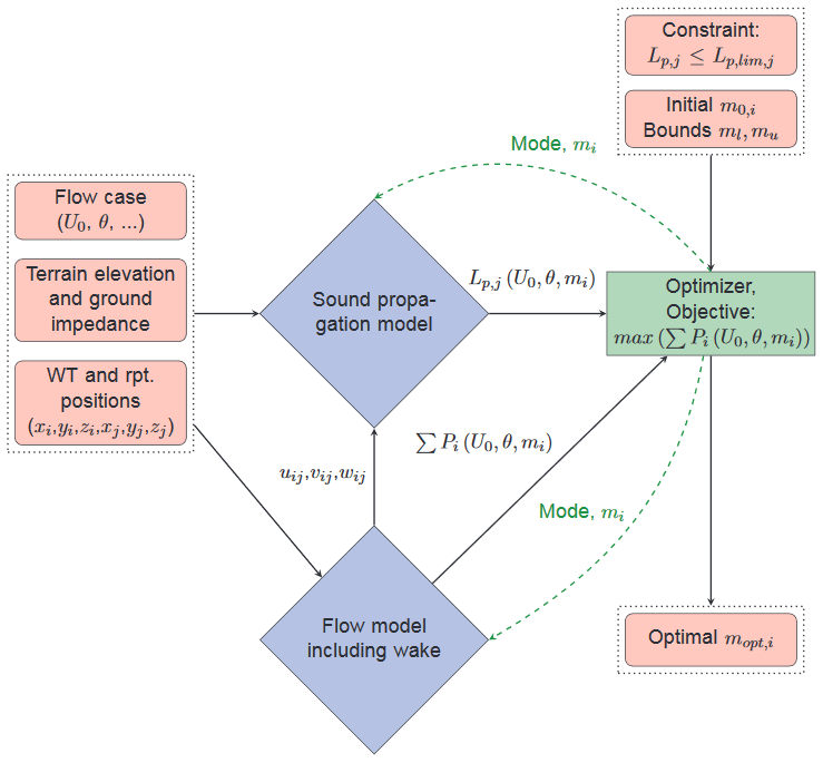
Figure 1Flow chart of the optimization framework structure. The flow chart can both be used for the ISO 9613-2 model and the WindSTAR model.
It is noted that for some wind speeds or wind directions it may be necessary to shut down a wind turbine completely if the operational modes do not provide the needed reduction in noise emission. Such a mode is, however, not included in the presented work. The updated operational mode, mi, of each wind turbine, i, is parsed into the wind farm model and the sound model in every iteration of the optimization, which in return parse the updated total power of the wind farm, , and the updated sound pressure level at each receptor, . Thus, the updated operational mode modifies the CT of the wind turbines and thereby the wakes through the wind farm, while the sound power level is likewise dependent on the operational mode causing a change in the integrated sound pressure level, Lp. The propagation of the sound itself is altered by the operational mode through the updated (uij, vij, wij) flow field parsed from the wind farm wake model to the sound propagation model. This step is only applicable for the WindSTAR model, since the ISO 9613-2 model does not take the entire flow field into account. It is later examined in Sect. 4.3 whether the sensitivity of the Lp,j provided by the WindSTAR model to the operational modes is negligible such that the sound propagation model alternatively can be computed only once prior to the optimization and used as a transfer function in each iteration. In this way, the computational time can be reduced considerably.
The flow chart can similarly be used to describe the optimization when the ISO 9613-2 model is applied to the sound propagation modelling. In this case only the effective wind speed at each wind turbine in the wind farm is needed from the (uij, vij, wij) field provided by the wind farm flow model to the sound model. Thus, since the flow field does not have any effect on the sound propagation obtained by the ISO 9613-2 model, it is only used in order to obtain the LW of the wind turbines. The flow case information and terrain elevation are still parsed as inputs to the ISO 9613-2 model as well. Thus, the terrain elevation is used to obtain the exact distances between the wind turbine hubs and the receptors. The ground impedance information is provided by the ground factor, G. Since the results from the ISO 9613-2 model are not depending on the flow field in the wind farm, the operational mode, mi, only changes the LW,i of each wind turbine. Thus, the propagation of the sound provided by the ISO 9613-2 model remains unchanged in each iteration.
4.1 Site and wind turbine types
For the optimizations done in this article, a wind farm in flat terrain is considered. For the layout of the wind turbines, the Lillgrund wind farm is used as a reference site. Although being an offshore wind farm, Lillgrund provides a flat terrain case consisting of a wind turbine type with various noise reducing operational modes. The Lillgrund wind farm has a size of 48 wind turbines, but only parts of the wind farm have been used for the tests performed in this work. Thus, the tests consider one row of the wind farm consisting of seven wind turbines and the north-east corner of the wind farm consisting of a layout of 4x5 wind turbines. Furthermore, artificial receptors, at which the noise constraints must be satisfied, are arbitrarily placed around the wind farm with a distance to the nearest wind turbine no closer than 4 times the total height of the wind turbine type.
The specifications of the wind turbine types used in this study are listed in Table 1.

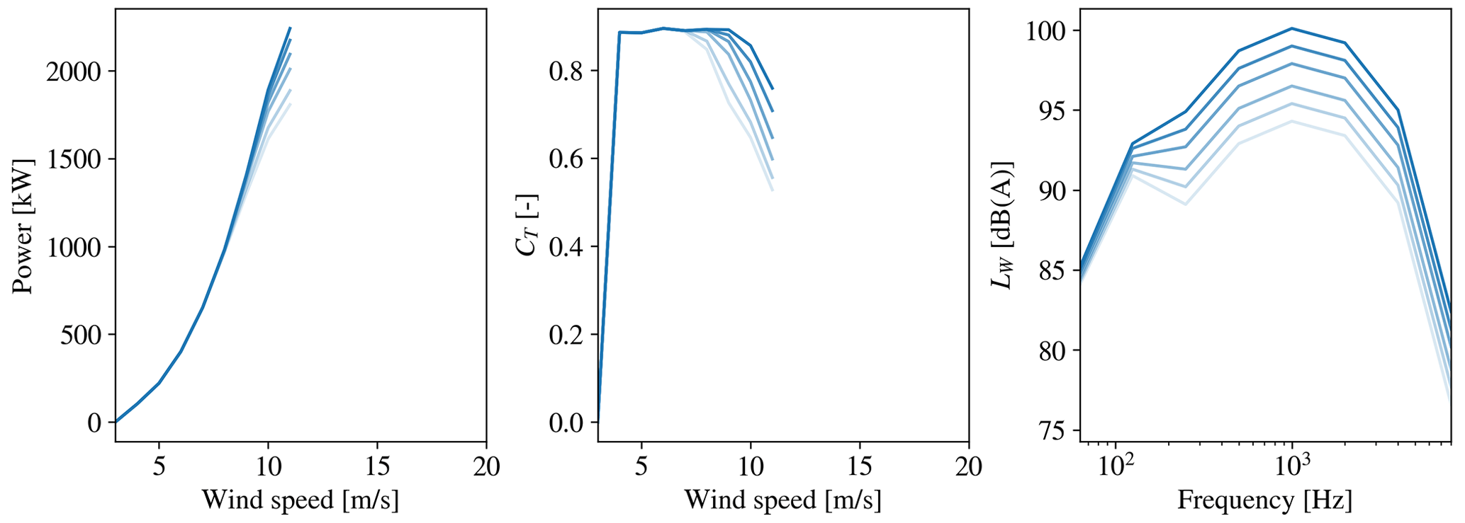
Figure 2SWT-2.3-93: the power, CT and LW curves for each operational mode at Uhub=10 m s−1. From dark to light blue is the least noise reducing mode, m=0, to the most noise reducing mode, m=6. Data are only available for wind speeds up to 11 m s−1 for this wind turbine.
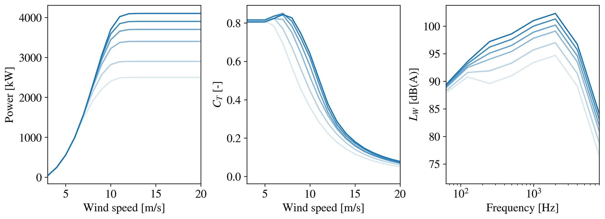
Figure 3SWT-DD-142: the power, CT and LW curves for each operational mode at Uhub=10 m s−1. From dark to light blue is the least noise reducing mode, m=0, to the most noise reducing mode, m=6.
The wind turbines in the Lillgrund wind farm are of the type Siemens SWT-2.3-93. A number of defined operational modes are provided for this wind turbine type with information about the LW spectra and the corresponding power and CT curves. The operational modes of the SWT-2.3-93 are, however, only given for hub height wind speeds up to 11 m s−1. Thus, additional optimizations using the larger Siemens SWT-DD-142 4.1 MW wind turbine are performed as well. The operational modes of the SWT-DD-142 turbine are defined for hub height wind speeds up to 20 m s−1, which allows for more exploration of the sensitivity of the Lp in a greater number of turbine operating conditions; moreover, the higher LW values of the larger turbine introduce a larger need for optimization. The power and CT curves as well as the LW spectra at Uhub=10 m s−1 are shown in Fig. 2 for the SWT-2.3-93 turbine and in Fig. 3 for the SWT-DD-142 turbine. For both turbine types a reduction in the LW at each octave band frequency as well as the corresponding power and CT is observed during the discrete steps from operational mode 0 to 6. It is further observed that the operational modes of the two turbine types introduce a similar reduction in LW while the power reduction is more distinct for the SWT-DD-142. The larger rotor diameter of the SWT-DD-142 requires a rescaling of the distance between the turbines in the chosen layouts. In the original layout using the SWT-2.3-93, the distance between turbines is 4.3 D in the direction from south-west to north-east and 3.3 D in the direction from north-west to south-east. These nondimensional distances are therefore used to scale the wind farm layout to fit the larger rotor diameter of D=142 m of the SWT-DD-142 turbine.
4.2 Test cases and constraints
For the initial tests of the optimization, the row of seven wind turbines either of the type SWT-2.3-93 or SWT-DD-142 is used. As mentioned, the distances between the turbines are scaled to fit the rotor diameter of the turbine type. As mentioned, four receptors are positioned in arbitrarily chosen locations but in such a way that some of the receptors will either be in the upwind or downwind positions of wind turbines in the farm. By choosing these positions, some of the distinct differences between the computed noise by WindSTAR and by ISO 9613-2 caused by refraction in the atmosphere are expected to be captured (Barlas et al., 2018). In the presented studies, two different wind directions are used, namely θ=0 and θ=225∘. In this way, the effect of all the wind turbines being in the free flow field compared to the majority of the wind turbines being in the wake of an upstream unit can be analysed. The temperature is T=15 ∘C and the relative humidity is ϕ=80 %. For the wind profile in the free field, a logarithmic profile for neutral conditions is used
where the roughness length is z0=0.1 m, the von Karman constant is κ=0.4 and the friction velocity is set to m s−1. The choice of parameters yield a hub height wind speed of Uhub=10 m s−1 for the SWT-DD-142 turbine with zhub=109 m and Uhub=9.3 m s−1 for the SWT-2.3-93 turbine with zhub=68.5 m. The ground flow resistivity used for computing the acoustic impedance is kept at kPa s m−2 (Wagner et al., 1996) in the WindSTAR model, while the remaining parameters of the Attenborough impedance model are defined by a pore shape factor of sp=0.75, a grain shape factor of , a porosity of Ω=0.3, a specific heat ratio of γ=1.4, a density of ρ=1.19 kg m−3 and the Prandtl number NPr=0.72. Correspondingly, the ground factor in the ISO 9613-2 model is kept at G=0 (DS, 1997). The chosen values for the ground parameters in both models are representative of a hard, reflecting ground. It is clear that using a hard, reflecting ground in the studies will lead to longer propagation of sound and higher noise levels in the far field of the wind turbines. Using instead a more absorbing ground with a lower ground flow resistivity would lead to a larger reduction in sound and thus lower noise levels at the considered receptors. We, however, keep the high ground flow resistivity to stay consistent with the Danish standard use of the ISO 9613-2 model.
In the final optimization of the presented work, the described layout of 4x5 wind turbines is considered. In this layout the larger SWT-DD-142 turbine is used. In a similar way as for the row of seven wind turbines, four receptors at different arbitrarily chosen positions near the wind farm are considered. The chosen layout results in individual WindSTAR computations. For the ISO 9613-2 model the 80 individual computations are performed in every iteration of the optimization. The noise constraint defined for the noise sensitive areas in Denmark is used for all receptors in all optimization cases presented. For the wind profile chosen, the wind speed at 10 m height is U10 m≈6 m s−1. The constraint is thus set to dB(A) (Nieuwenhuizen and Köhl, 2015). Lastly, the initial mode of every wind turbine is set to , starting the optimization from the least noise reducing mode. As a result of the study done in Sect. 4.3, the optimization with the WindSTAR model is performed by conducting the initial sound propagation computations for the specified flow cases and using the results as a transfer function for all wind farm layouts in this article.
4.3 CT sensitivity of WindSTAR
A large downside of the current optimization framework is the computational time. Thus, since the main contributor to the long computational time of the optimization framework is the computations of the sound propagation in WindSTAR, it is tested whether the sensitivity of WindSTAR results to the updated operational mode, mi, is significant or not. Since the sound propagation depends on the flow field, and thereby the CT of the wind turbines producing the flow field, mi is expected to directly affect the sound propagation. The sensitivity of the operational modes studied here does therefore not include the LW of the wind turbines, since this parameter is not influenced by the WindSTAR computations. The CT (or mi) sensitivity study of WindSTAR is done by considering two simple setups both in flat terrain. The two setups are sketched in Fig. 4.

Figure 4(a) Setup 1 with the downwind attenuation of sound from a single wind turbine at different operational modes. (b) Setup 2 with the downwind attenuation of sound from a single wind turbine in the wake of a wind turbine at different operational modes. The distance between the two wind turbines is d≈3.8 D.
The first setup considers one wind turbine with a receptor line positioned in the wake and reaching 3 km from the wind turbine. The operational mode of the wind turbine is thus switched between mode 0, 3 and 6 for different hub height wind speeds: 6, 10 and 14 m s−1 and the wind speed profile given in Eq. (8). The ground conditions are similar to the ones described in Sect. 4.2 for a flat terrain. The second setup considers two wind turbines with one wind turbine positioned in the wake of the other and the receptor line positioned in the wake of the rear turbine and reaching 3 km away. The distance between the two turbines is d≈3.8 D, where D is the rotor diameter of the wind turbines. With the layout of the Lillgrund wind farm in mind, this is expected to be a realistic distance. In this case the operational mode of the front wind turbine is switched in a similar way as in the first setup. The purpose of the second setup is to investigate the effect of changing the effective wind speed at the rear wind turbine. For each setup the largest turbine type, SWT-DD-142, is used. This is chosen due to the larger modifications of the power and CT curves observed when changing the operational mode in Fig. 3. By using the two defined cases, the sensitivity of the TL from a wind turbine operating at different modes and the TL from a wind turbine in the wake of another wind turbine operating at different modes can be investigated. Only cases with the receptor in the downwind/wake position of the wind turbines are considered, since the CT is only causing changes in the wake and not the free flow field in the upwind or crosswind position of the wind turbines. This is a result of using an engineering wake model in the framework. The range-dependent TL for the different operational modes including the geometrical spreading, the relative sound pressure level and the atmospheric absorption are shown for the first setup in Fig. 5 and for the second setup in Fig. 6. The atmospheric absorption is estimated for T=15 ∘C and ϕ=80 %. The computations in these figures are all obtained at Uhub=10 m s−1, while the results for Uhub=6 and Uhub=14 m s−1 are presented in Appendix A.
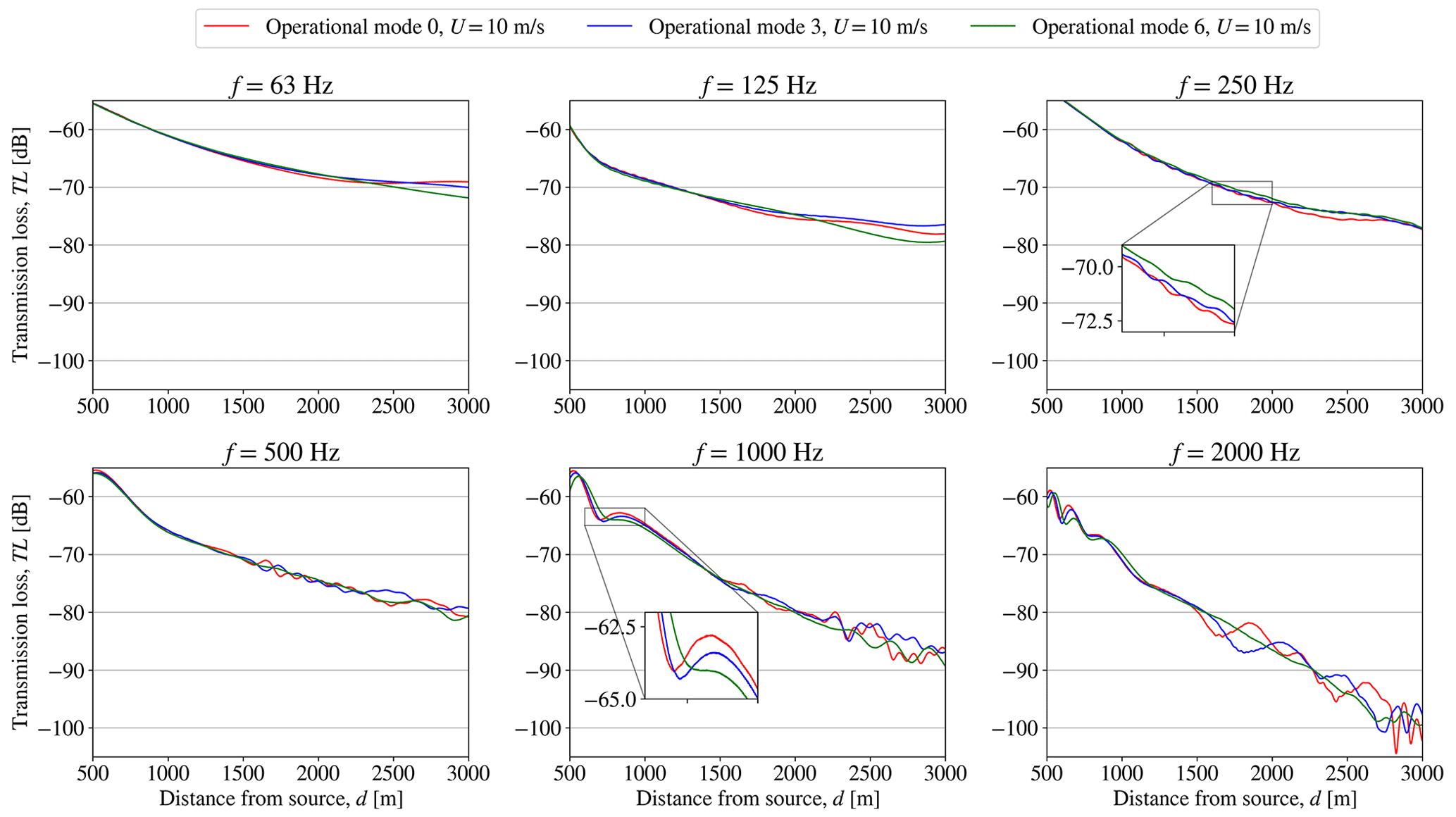
Figure 5Setup 1: the transmission loss, TL, obtained from WindSTAR computations from a single SWT-DD-142 wind turbine subject to changing operational modes at each octave band frequency at a free field wind speed of Uhub=10 m s−1 at hub height.
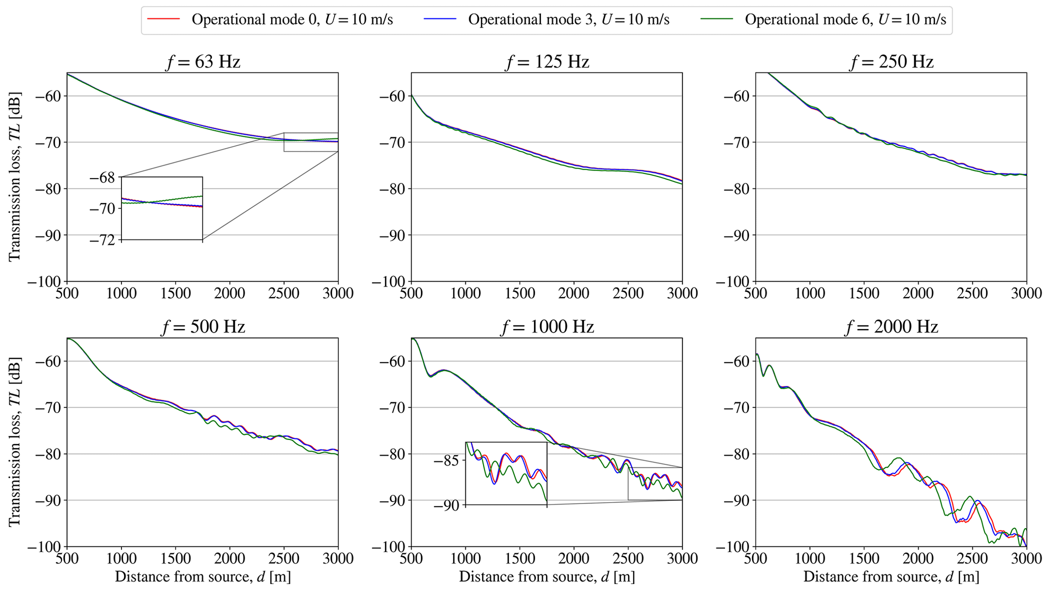
Figure 6Setup 2: the transmission loss, TL, obtained from WindSTAR computations from a single SWT-DD-142 wind turbine positioned in the wake of a wind turbine subject to changing operational modes at each octave band frequency at a free field wind speed of Uhub=10 m s−1 at hub height.
In the results presented in Fig. 5, it is observed how the range-dependent TL at each octave band frequency, fk, is altered as the operational mode of the wind turbine is switched. However, the effect of the change in operational mode is mostly observed in the far field of the wind turbine at distances longer than d=2 km. Moreover, the effects become more apparent for higher frequencies of f=1 and f=2 kHz with significant differences appearing after d=1500 m for f=2 kHz and after d=2000 m for f=1 kHz. In Fig. 6 the effect on the propagation from a wind turbine in the wake of another turbine subject to changes in operational mode can be observed. The changes in the TL are generally seen to be less significant than the ones observed for the first setup in Fig. 5. The most distinct differences are observed when switching the front wind turbines from mode 3 to mode 6. Still, the major effects are apparent at further distances and higher frequencies. When observing the TL at Uhub=6 and 14 m s−1 in Figs. A1–A4, the sensitivity of the change in operational modes is less significant at Uhub=6 m s−1. At U0=14 m s−1, the TL shows changes in the far field similar to Figs. 5 and 6. It is observed that, especially for some frequencies at Uhub=6 m s−1, the results obtained for mode 0 and mode 3 are similar, making mode 0 hardly noticeable in Figs. A1 and A3. Since the sensitivity to the operational modes in the presented cases is generally observed for longer distances at higher frequencies, the contribution to the overall sound pressure level is concluded to be negligible compared to the observed high transmission losses. The sound propagation modelling in WindSTAR can therefore be excluded from the iterative function calls during the optimization and instead performed separately prior to the optimization by using the initial modes, m0,i, of the wind turbines. The TL obtained from the initial run of WindSTAR is therefore used as a transfer function in the optimizations presented in this article.
5.1 Row of seven wind turbines
As mentioned, the optimization of the wind farm operation is done for both a row of seven SWT-2.3-93 turbines and a row of seven SWT-DD-142 turbines. The flow fields through the row of wind turbines for the chosen flow cases with the two different wind directions θ=0 and θ=225∘ are observed for the SWT-DD-142 wind turbine in Figs. 7 and 12. Figures of the flow fields for the SWT-2.3-93 turbines are not included here, since the layout is very similar to the row of SWT-DD-142 turbines. It is noticed that the four receptors will be in either the upwind, downwind or crosswind positions of the wind turbines depending on the wind direction. For θ=0∘, two receptors are positioned directly in the wake of a wind turbine, while the two remaining receptors are positioned in the free flow field directly upwind of a wind turbine. For θ=225∘ all receptors are positioned in the free flow field either dominantly downwind or upwind of the wind turbines.
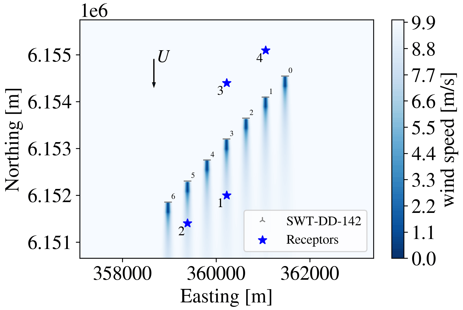
Figure 7The flow field at hub height through the row of seven SWT-DD-142 wind turbines at the wind direction θ=0∘. The distances between the turbines are scaled to be approximately 4.3 D.
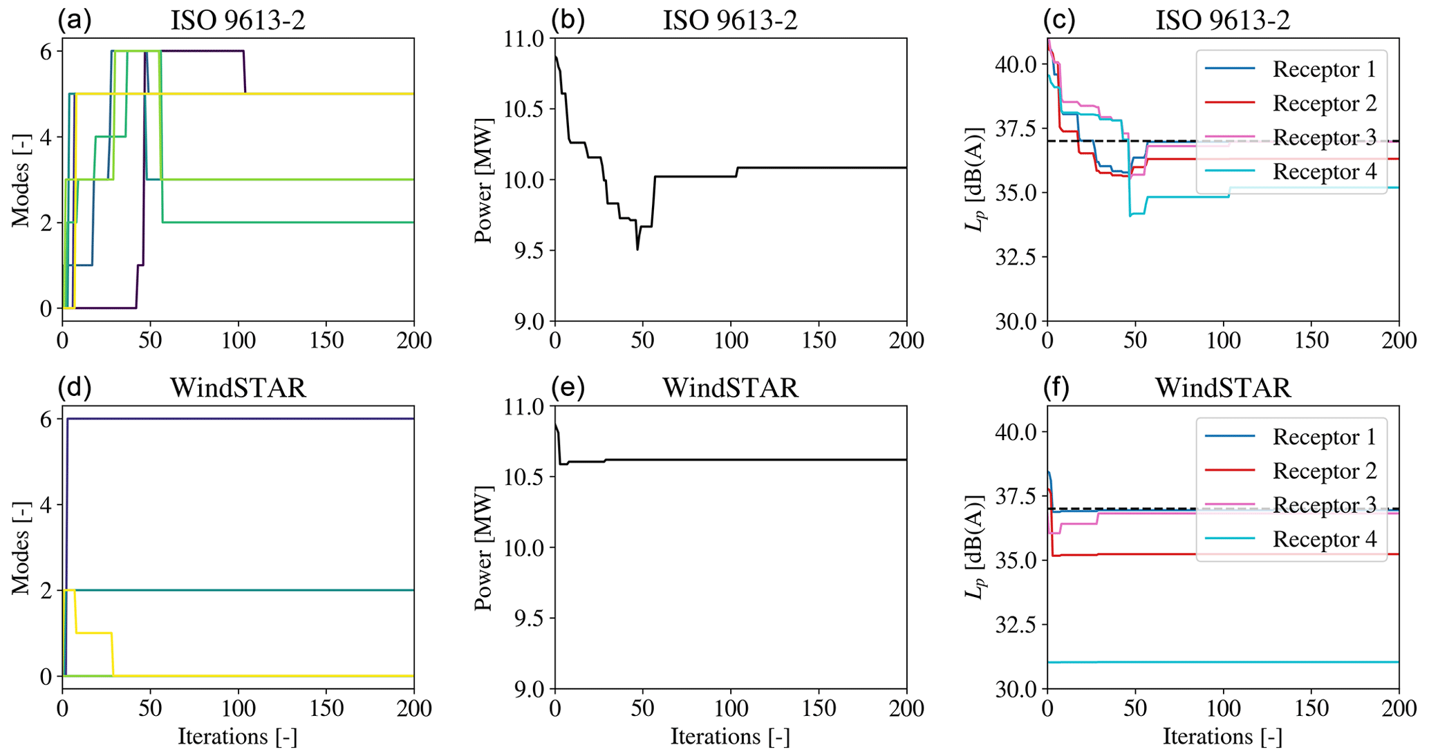
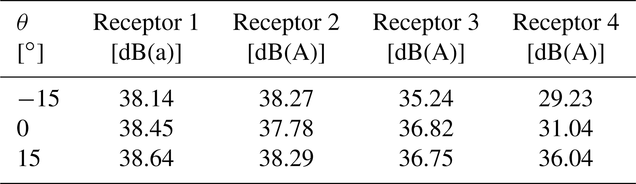
Figure 8The operational mode, mi, for each wind turbine (a, d); the overall power, P, of the row of seven SWT-2.3-93 wind turbines (b, e); and the integrated sound pressure level, Lp,j, at each receptor (c, f) during the optimization at θ=0∘ and Uhub=9.3 m s−1. The noise constraint is set to dB(A) and represented by the dashed line in the right figure.
The convergence of the total power output; the operational modes of each wind turbine, mi; and the Lp,j at each receptor during the optimization performed for the flow case of are shown in Fig. 8 for the seven SWT-2.3-93 turbines. For all presented wind farm layouts and flow cases the convergence is shown for both the optimization using the ISO 9613-2 model and for the one using the WindSTAR model outside of the iterative function calls. A total number of 1000 iterations have been chosen for the optimization, but it is observed that convergence is reached after around 100 iterations for the ISO 9613-2 model and after 50 iterations for the WindSTAR model. Thus, the optimization is observed to converge relatively fast. It is observed how the ISO 9613-2 model is generally predicting higher Lp,j values than the WindSTAR model at the initial operational mode, m0,i. This could be the cause of the larger number of iterations needed to reach convergence and a lower optimized power output of the wind farm. It is observed how the optimization with the ISO 9613-2 model first overcompensates for the violated constraint and eventually increases the Lp,j at all receptors to approach the , thus increasing the power output of the wind farm. The WindSTAR model predicts significantly lower Lp,j for all receptors causing only a few of the turbines to switch to a noise reducing mode.
Scatter plots of the operational modes of each wind turbine along with the corresponding Lp,j before, during and after the optimization are given in Fig. 9. The scatter plot at the time during the optimization represents the iteration at which the estimated power output is at its minimum. The receptors at which the noise constraint is violated are coloured red, while the ones at which the constraint is satisfied are blue. It is noticed how Lp,j estimated by ISO 9613-2 model is estimated to violate the constraint at the initial mode, m0,i. When observing the WindSTAR results for m0,i, two receptors are estimated to experience Lp,j values lower than the constraint. One receptor positioned in the upwind of all wind turbines, especially, is exposed to a significantly reduced Lp,j as a result of upward refraction. It is however noted that the uncertainty of WindSTAR in the shadow zone might be significantly higher due to the fact that turbulence is omitted. Thus, a higher Lp,j could be expected at these positions due to scattering of sound into the shadow zone. It should be kept in mind that shadow zones in the upwind positions of wind turbines cannot be generalized to all cases, as shown by Barlas et al. (2017). Here, it is seen that for some distances upwind of a wind turbine, a higher Lp,j is experienced. However, for the cases considered in our work presented in this article, shadow zones are observed for the upwind positions. In general, it should be kept in mind for all optimization cases that the optimizations are done for a single wind direction and wind speed, which in this case causes two receptors to be directly upwind. Thus, normally a small variation in, i.e. the wind direction would be expected for each considered flow case. The effect of varying the wind direction in the WindSTAR model is shortly investigated for in Table 2. Observing receptor 3 and 4, the Lp,j is further reduced when considering ∘ since the positions of the receptors become even more upwind relative to the closest wind turbine. At ∘ the position of receptor 4 relative to the closest turbine is more crosswind resulting in a distinct increase in Lp,j. On the other hand, receptors 1 and 2 experience smaller variations in the Lp,j with the change in θ. Thus, the more abrupt changes in sound propagation appear when receptors are in the upwind position. It should be noted that these variations only appear in the WindSTAR results since the propagation of the ISO 9613-2 model is not sensitive to changes in the wind direction when the wind turbines are positioned in the free field.
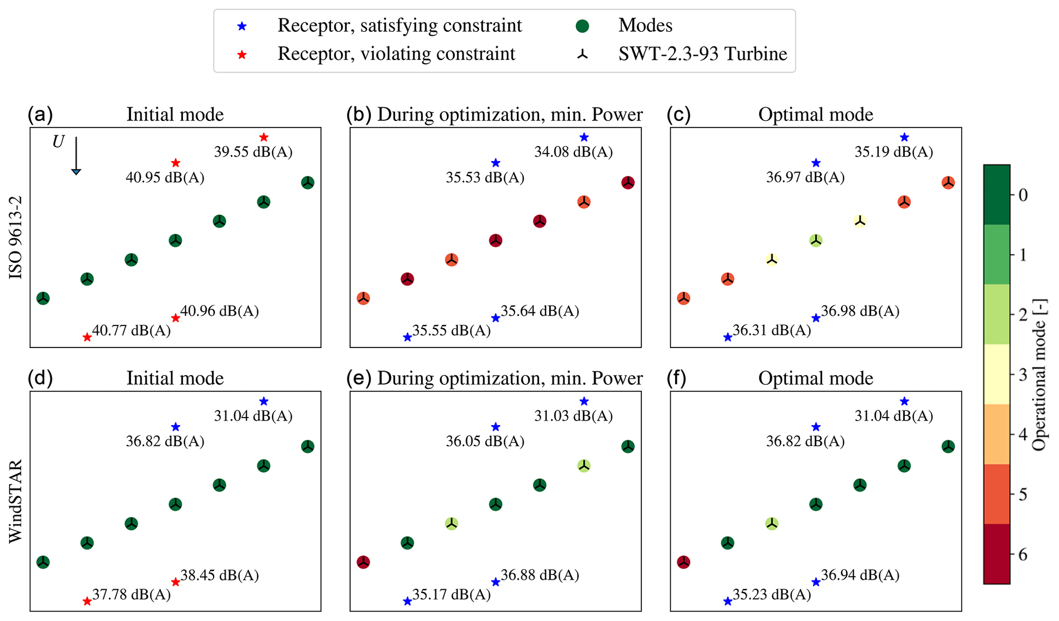
Figure 9Scatter plots of the operational modes of the seven SWT-2.3-93 wind turbines before (a, d), at the minimum power iteration during (b, e) and after (c, f) the optimization at θ=0∘ and Uhub=9.3 m s−1. The noise constraint is set to dB(A).
Table 2Overall Lp,j estimated by WindSTAR at each receptor for for the row of seven SWT-2.3-93 wind turbines operating at mi=0.
During the optimization it is observed that the noise reducing modes are distributed to all wind turbines when using the ISO 9613-2 model, while the WindSTAR optimization only modifies two–three turbines. For the optimum, all wind turbines are switched to a noise reducing mode in the ISO 9613-2 optimization while the operation of only two turbines, close to the receptors initially being subject to constraint violations, is modified in the WindSTAR optimization. For the ISO 9613-2 optimal mode it is observed that the turbines in the outer positions of the row have the highest curtailment while the turbines in the centre are less noise curtailed. This occurs even though the receptors closest to the centre of the row initially are exposed to the highest Lp,j.
Convergence plots are similarly presented for the optimization of the row of seven SWT-DD-142 turbines in Fig. 10 at θ=0∘. In general, a slightly higher Lp,j are experienced for all receptors due to the increased turbine size. It is observed that during the ISO 9613-2 optimization, the operational modes are gradually modified causing receptor 1, 2 and 4 to quickly reach Lp,j values below the constraint. However, although the Lp,j of receptor 3 initially is at the same level as the Lp,j at receptor 1 and 2, it is not as significantly reduced with the change of operational modes. Thus, the power output is seen to reach a certain level at which the constraints are satisfied and after this point not being able to optimize any further. The large curtailment in order to bring the Lp,j of receptor 3 below 37 dB(A) further causes the remaining receptors to experience an Lp,j significantly below the constraint. For the WindSTAR optimization the Lp,j at all receptors is on the other hand kept close to the constraint. Thus, although the Lp,j at receptor 3 is just below 37 dB(A), in the further iterations the optimizer still manages to find a more optimal solution that increases the power output.
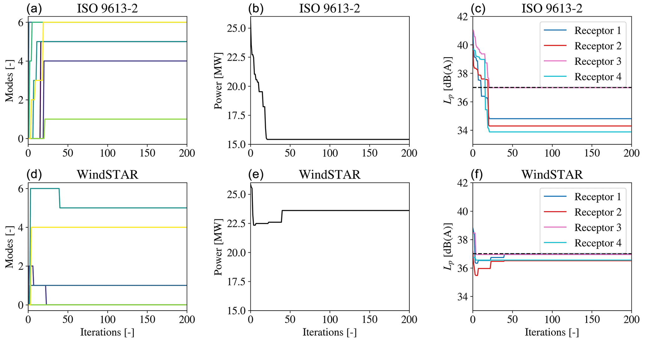
Figure 10The operational mode, mi, for each wind turbine (a, d); the overall power of the seven SWT-DD-142 wind turbines (b, e); and the integrated sound pressure level, Lp,j, at each receptor (c, f) during the optimization at θ=0∘ and Uhub=10 m s−1. The noise constraint is set to dB(A) and represented by the dashed line in the right figure.
The scatter plot in Fig. 11 emphasizes the observations done in the convergence plots in Fig. 10. Thus, it is apparent that a higher Lp,j is generally computed at each receptor. The Lp,j at receptor 2, which for the SWT-2.3-93 turbine type was estimated by the WindSTAR model to be slightly below 37 dB(A), is now violating the noise constraint. Moreover, receptor 1 with a significantly lower Lp,j in Fig. 9, which was expected to be caused by a shadow zone in the upward refracting atmosphere captured by WindSTAR, is observed to receive an Lp,j similar to the Lp,j estimated at the remaining receptors. This can be a result of the increased hub height when going from the SWT-2.3-93 to the SWT-DD-142 turbine, yielding an increased height of the source positions. The higher source positions is expected to thereby cause the sound waves to travel further before attenuating due to the upward refraction (Bolin et al., 2020). Furthermore, the three point sources are distributed over a larger area due to the increased rotor diameter. Thus, averaging over points that are further apart could further cause the effect from the shadow zone to be reduced. For the optimization using the ISO 9613-2 model it is observed how three of the wind turbines are switched to the most noise reducing mode, mi=6, and only one wind turbine is kept at mi=0. The power output is thereby heavily curtailed in order to satisfy the noise constraint. The corresponding optimization with the WindSTAR model results in a higher power output due to the estimated lower Lp,j.

Figure 11Scatter plots of the operational modes of the seven SWT-DD-142 wind turbines before (a, d), at the minimum power iteration during (b, e) and after (c, f) the optimization at θ=0∘ and U0=10 m s−1. The noise constraint is set to dB(A).
The optimization of the row of seven turbines is further performed for a flow case with a wind direction of θ=225∘. The resulting flow field in the plane at hub height is presented in Fig. 12 for the SWT-DD-142 turbines. The choice of wind direction results in the majority of the wind turbines being positioned in a wake field. This will cause reduced effective wind speeds, presumably leading to a lower Lp,j at the receptors. Furthermore, none of the receptors are positioned directly in the wake or directly upwind of a turbine. Hence, they are all positioned in a free flow field.
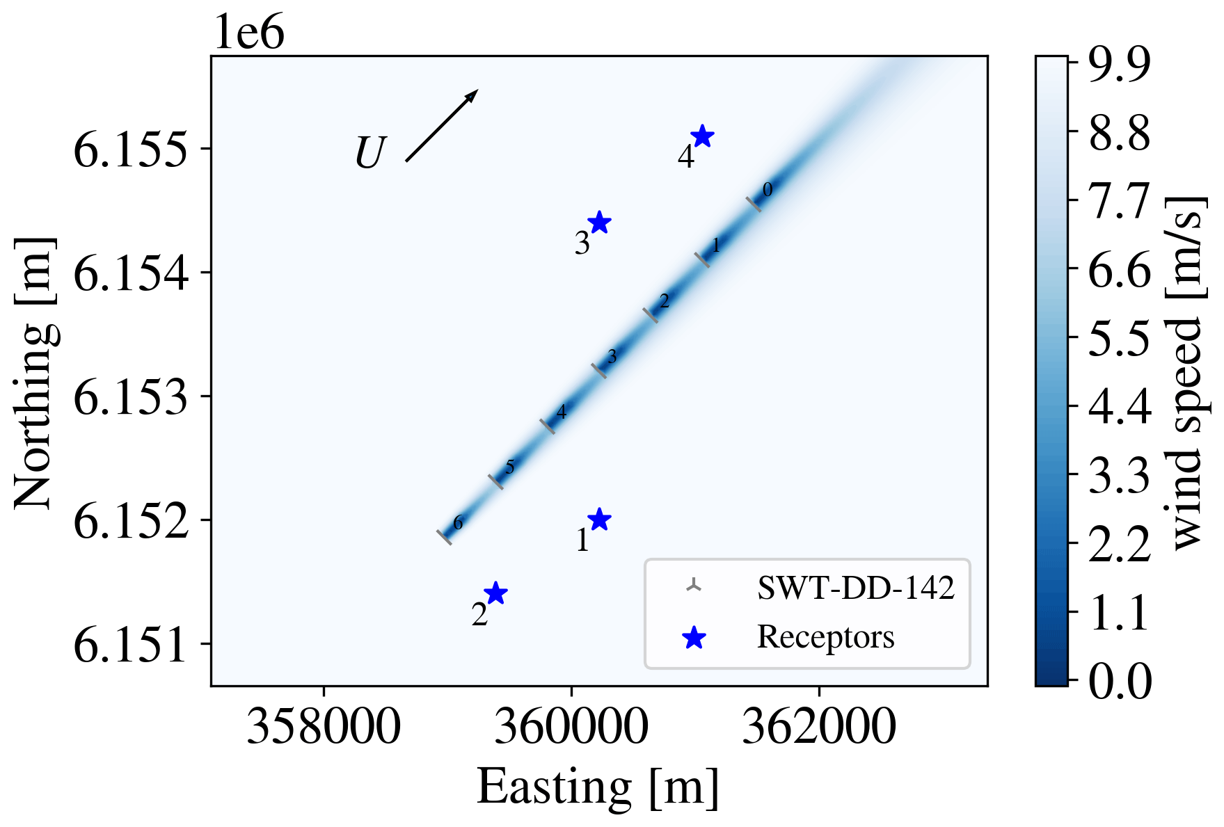
Figure 12The flow field at hub height through the row of seven SWT-DD-142 wind turbines at the wind direction θ=225∘. The distances between the turbines are scaled to be approximately 4.3 D.
When comparing the convergence for the SWT-2.3-93 turbine in Fig. 13 with the convergence for the SWT-DD-142 turbine in Fig. 14, both at θ=225∘, some noticeable differences can be observed. Similar to the flow case of θ=0∘, the optimization using the SWT-2.3-93 turbine and the ISO 9613-2 model yields reduced modes for a majority of the wind turbines in the optimized solution. It is noticed how the Lp,j at receptors 3 and 4 positioned downstream along the row of turbines is significantly lower when θ=225∘. This is caused by the reduced effective wind speed, Ueff, of the nearest wind turbines since they are now in a wake position. This reduction is more apparent when observing the WindSTAR optimization in which the Lp,j at receptor 3 and 4 is well below the defined noise constraint. Receptors 1 and 2, positioned more upstream of the row of wind turbines, are however still exposed to higher Lp,j, which for the ISO 9613-2 optimization results in the observed mode reduction. For the WindSTAR optimization, only the Lp,j at receptor 1 is violating the noise constraint leading to only two of the wind turbines operating at noise reducing modes.
A different behaviour of the optimizer is noticed when considering the row of SWT-DD-142 turbines in Fig. 14. Thus, it is observed that as the turbine operation is modified to a noise reducing mode, the power output increases. This is caused by the reduced CT at the noise reducing modes leading to a higher Ueff at the rotor positioned in the wake. Thereby, although the front turbine will produce a decreased amount of power, the overall output of the wind farm will be improved. This optimization also yields a significant decrease in the Lp,j at each receptor, automatically keeping it below the noise constraint. This tendency of the optimization is only obtained for the larger turbine type, which is expected to be caused by the larger differences in the power and CT curve observed for the SWT-DD-142 turbine at Uhub=10 m s−1 in Fig. 3 than for the SWT-2.3-93 turbine at Uhub≈9.3 m s−1 in Fig. 2. Hence, the differences between the CT curves for each of the operational modes defined for the SWT-2.3-93 may not be significant enough to cause a higher overall power output of the wind farm.

Figure 13The operational mode, mi, for each wind turbine (a, d); the overall power of the seven SWT-2.3-93 wind turbines (b, e); and the integrated sound pressure level, Lp, at each receptor (c, f) during the optimization at θ=225∘ and Uhub=9.3 m s−1. The noise constraint is set to dB(A) and represented by the dashed line in the right figure.

Figure 14The operational mode, mi, for each wind turbine (a, d); the overall power of the seven SWT-DD-142 wind turbines (b, e); and the integrated sound pressure level, Uhub=10 m s−1, at each receptor (c, f) during the optimization at θ=225∘ and U0=10 m s−1. The noise constraint is set to dB(A) and represented by the dashed line in the right figure.
5.2 4×5 wind turbines layout
Lastly, the larger wind farm layout of 4×5 wind turbines is tested by using the SWT-DD-142 turbine. The larger wind turbine type is chosen due to the more distinct differences in the defined operational modes seen in Fig. 3. The flow field including the wind turbine wakes through the wind farm are shown in Fig. 15 with θ=0∘. Similar to the row of seven wind turbines analysed thus far, 4 receptors are arbitrarily positioned around the wind farm. As can be noticed in Fig. 15, the receptors are positioned downwind, upwind or crosswind of the wind turbines.
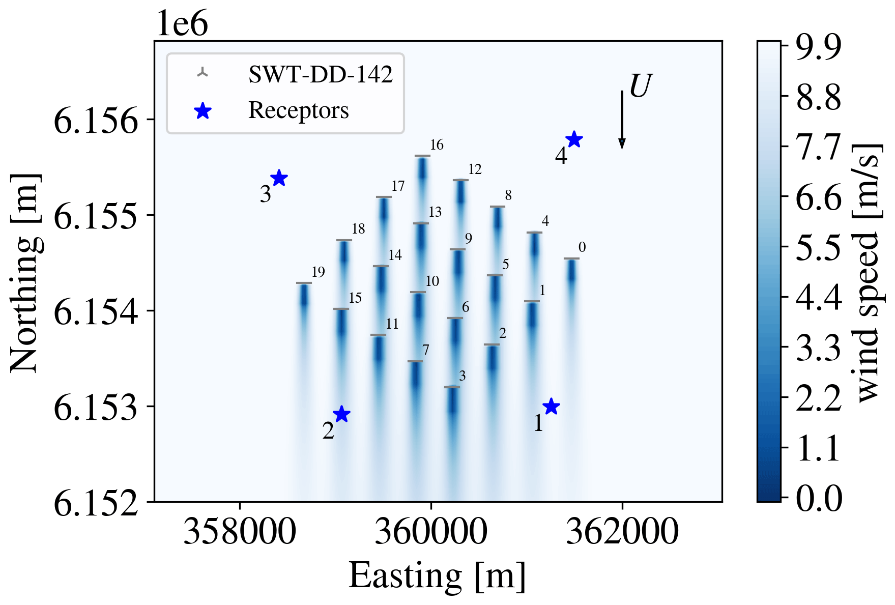
Figure 15Example of flow at hub height through the 4×5 SWT-DD-142 wind turbines at the wind direction θ=0∘. The distances between the turbines are scaled to be approximately 4.3 and 3.3 D.
The convergence of the ISO 9613-2 and WindSTAR optimization, respectively, of the 4x5 wind farm is presented in Fig. 16 and scatter plots are shown in Fig. 17. It is observed that for both the ISO 9613-2 and the WindSTAR model, the optimizer uses more iterations before reaching convergence due to the increased number of design variables. As has been discussed for the row of seven wind turbines, the WindSTAR model generally estimates a lower Lp,j at all receptors than the ISO 9613-2 model. It is further noticed that even though the size of the wind farm has increased significantly, the Lp,j is still similar to the Lp,j estimated at the row of turbines. Hence, the noise characteristics of the nearest wind turbines seem to have a larger impact on the received Lp,j than the total number of noise sources does. The upwind positions of some of the receptors are further seen to not significantly affect the Lp,j estimated by WindSTAR, which is expected to be due to the contribution from the remaining wind turbines nearby. The higher Lp,j estimated by the ISO 9613-2 model causes the wind turbines to be generally heavily curtailed. It is observed how at the iteration evaluating the minimum power output, the heavily noise reducing modes are distributed to all turbines in the wind farm. At the end of the optimization, the turbines positioned at the edges of the wind farm are more heavily curtailed, while the centre turbines are modified to lower operational modes. Although the Lp,j is estimated by WindSTAR to violate the noise constraint at almost all receptors at the initial operational mode , the WindSTAR optimization still manages to reach a power output very close to the initial power output. The computed Lp,j at receptor 4 positioned upwind of the wind farm is just below the noise constraint of 37 dB(A), resulting in the upper right row of turbines closest to receptor 4 proceeding to operate at the initial m0,i.
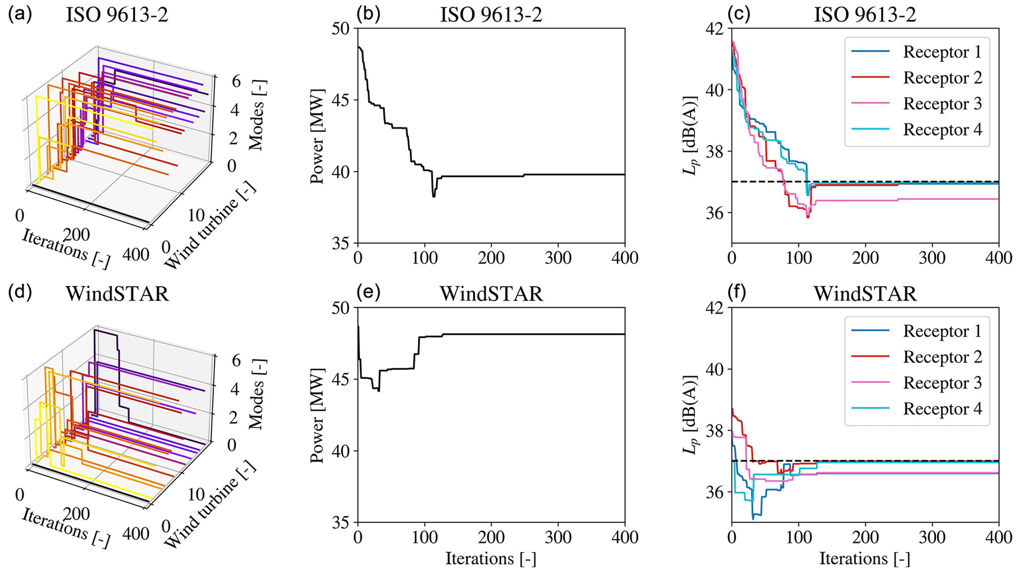
Figure 16The operational mode, mi, for each wind turbine (a, d); the overall power of the 4×5 SWT-DD-142 wind turbines (b, e); and the integrated sound pressure level, Lp,j, at each receptor (c, f) during the optimization at θ=225∘ and Uhub=10 m s−1. The noise constraint is set to dB(A) and represented by the dashed line in the right figure.
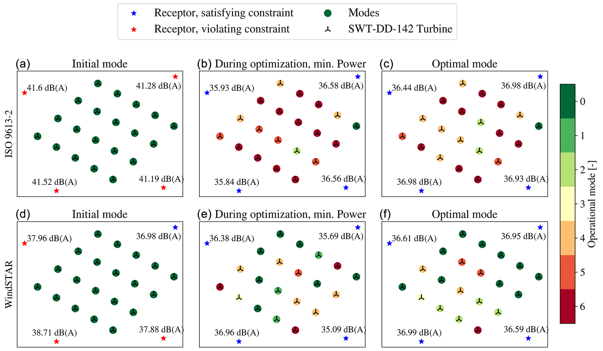
Figure 17Scatter plots of the operational modes of the 4×5 SWT-DD-142 wind turbines before (a, d), at the minimum power iteration during (b, e) and after (c, f) the optimization at θ=0∘ and U0=10 m s−1. The noise constraint is set to dB(A).
5.3 Further discussion
In the optimizations performed in the presented work, the optimization method using a random search algorithm has been applied (Feng and Shen, 2015, 2017). The method is compatible with optimization problems of discrete design variables, and by being a global search algorithm, it is more certain to find the global minimum/maximum. However, as briefly mentioned, the method has the disadvantage of getting less efficient as the size of the wind farm in question, the number of receptors or the number of possible operational modes increases. Therefore, it can be beneficial to use a gradient-based optimization method for the defined problem (Martins and Ning, 2021). The gradient-based approach requires that the functions in the optimization can be assumed to be continuous such that the gradient of the ISO 9613-2 model and the WindSTAR model, respectively, as well as the overall power output of the wind farm obtained from PyWake with respect to the discrete operational modes can be derived. By doing so, the optimization method using the WindSTAR model can be applied to larger problems and to a broader range of flow cases in order to obtain an estimate of the optimized AEP. Applying gradient-based optimization to a discrete variable optimization problem has earlier been done by Pollini (2022). It should however be noted that the optimizations presented in this article are considered a “proof of concept” of the developed approach to optimize the wind farm operation based on the advanced sound propagation modelling. The use of the random search algorithm is therefore concluded to be a feasible choice for this purpose. This had been further emphasized through this article by the fast convergence of the presented optimization studies.
The use of any of the two sound propagation models introduces an uncertainty to the predicted sound pressure level at each receptor. First of all, both the WindSTAR model and the ISO 9613-2 model compute the sound propagation based on simplified flow fields using a logarithmic inflow profile and an engineering wake model. Thus, these simplifications introduce uncertainties already in the flow field modelling, which is expected to propagate as uncertainties in the sound propagation modelling. It should however be noted that the use of the logarithmic inflow profile is deemed acceptable for the flat terrain in the studied wind farm cases. For a complex terrain wind farm, higher fidelity flow modelling like RANS should be considered in order to obtain the speed-ups in the flow field. In addition, the turbulence effects in the atmosphere are neglected due to the high computational costs. This will in some scenarios, i.e. when considering receptors in the upwind position of a wind turbine, lead to higher uncertainties due to the omitted scattering of sound. Turbulence can further have a significant impact on the noise generation at the wind turbine rotor, which is not accounted for by the noise reducing operational modes of the turbine. The turbulence effects in the sound propagation modelling of WindSTAR could be included by, i.e. developing a surrogate model based on a limited amount of model evaluations (Martins and Ning, 2021). Thus, the turbulence effects will be introduced in future work.
In general the ISO 9613-2 model is observed to estimate higher sound pressure levels at the different receptors compared to the WindSTAR model. Although this suggests that the ISO 9613-2 model is more conservative, it on the other hand gives a higher insurance that the noise constraints are not violated. Thus, the lower estimated sound pressure level of WindSTAR may lead to that the noise constraints in reality are not satisfied at the obtained optimal mode. This could, i.e. be accounted for by adding the uncertainty of the WindSTAR model to the integrated sound pressure levels prior to the optimization. However, in general the higher fidelity model gives a better prediction of the noise at each receptor and allows for a broader exploration of the flow parameters and their influence on the Lp,j.
Through the work of this article a new approach for performing optimization of wind farm operation was presented. The optimization considers noise constraints at nearby receptors of an onshore wind farm. By the use of the ISO 9613-2 and WindSTAR sound propagation models as well as the Topfarm optimization framework and PyWake flow model the overall power output is optimized in a specific flow case while assuring that the sound pressure level satisfies the given noise constraints. This is done by individually changing the defined operational modes of each wind turbine in the wind farm. The approach was tested on a smaller wind farm of seven wind turbines and four receptors, which showed a fast convergence for both sound propagation models and a significant gain in power output when using the WindSTAR model over the ISO 9613-2 model. Especially for cases in which one or more receptors are in the upwind positions of the wind farm, the use of the WindSTAR model in the optimization results in lower estimated sound pressure levels at the receptors and a higher overall power output of the wind farm. While being a more advanced sound propagation model, it is also evident that the use of the WindSTAR model requires longer computational times. It was therefore tested whether the sensitivity of the WindSTAR model to the operational modes is negligible, such that the WindSTAR computations can be performed once prior to the optimization and later used as a transfer function during the iterations in the optimization. It was shown that variations in the sound attenuation are most apparent for far distances where the sound pressure levels are already low. These variations were therefore omitted and WindSTAR was used as a transfer function. As an analysis for future work with the presented framework, the potential and uncertainty in replacing WindSTAR computations at the cases of high frequencies and long distances with ISO 9613-2 computations will be investigated. This is already done for frequencies and distances where the memory of the computations becomes too excessive. However, there is a potential value in implementing this replacement at shorter distances for f=1 and f=2 kHz and thereby ideally reducing the computational time even further.
As the optimization is performed for a single flow case with constant wind speed profile, wind direction, temperature profile and ground conditions, this can lead to uncertainties when applied to the operation of the wind turbines during, e.g. a day. Thus, the sound propagation achieved especially from WindSTAR is sensitive to the flow and temperature in the wind farm which experience frequent changes and the ground acoustic impedance which can experience seasonal changes (for example going from snow covered terrain in the winter to grass covered in the summer). Thus, to obtain the full operational strategy of a wind farm, a structured sensitivity study of WindSTAR with respect to these parameters is needed.
Finally, the optimization framework has been tested on an artificial onshore wind farm of the size of 4x5 SWT-DD-142 4.1 MW wind turbines and four nearby receptors. Although being a larger wind farm, both sound propagation models show that the sound pressure levels at each receptor do not necessarily increase, implying that the noise characteristics of the nearest wind turbines are of higher importance than the number of turbines in the considered wind farm.
As it has been discussed, the use of a random search algorithm for the optimization does not guarantee a global optimum. In order to fully exploit the capabilities of the framework and to further approach a globally optimal solution, a gradient-based approach should be implemented. This requires that the gradient of the sound pressure level at each receptor with respect to the operational modes of each wind turbine is derived. Thus, this is considered the next step in the development of the framework.
In extension to the study done in Sect. 4.3, this Appendix presents analysis figures of the thrust coefficient, CT, sensitivity of WindSTAR. Thus, to represent the different operation stages of the wind turbines, Figs. A1 and A3 present the sensitivity study for a hub height wind speed below rated, U0=6 m s−1, while Figs. A2 and A4 present the study for a wind speed well above rated, U0=14 m s−1.
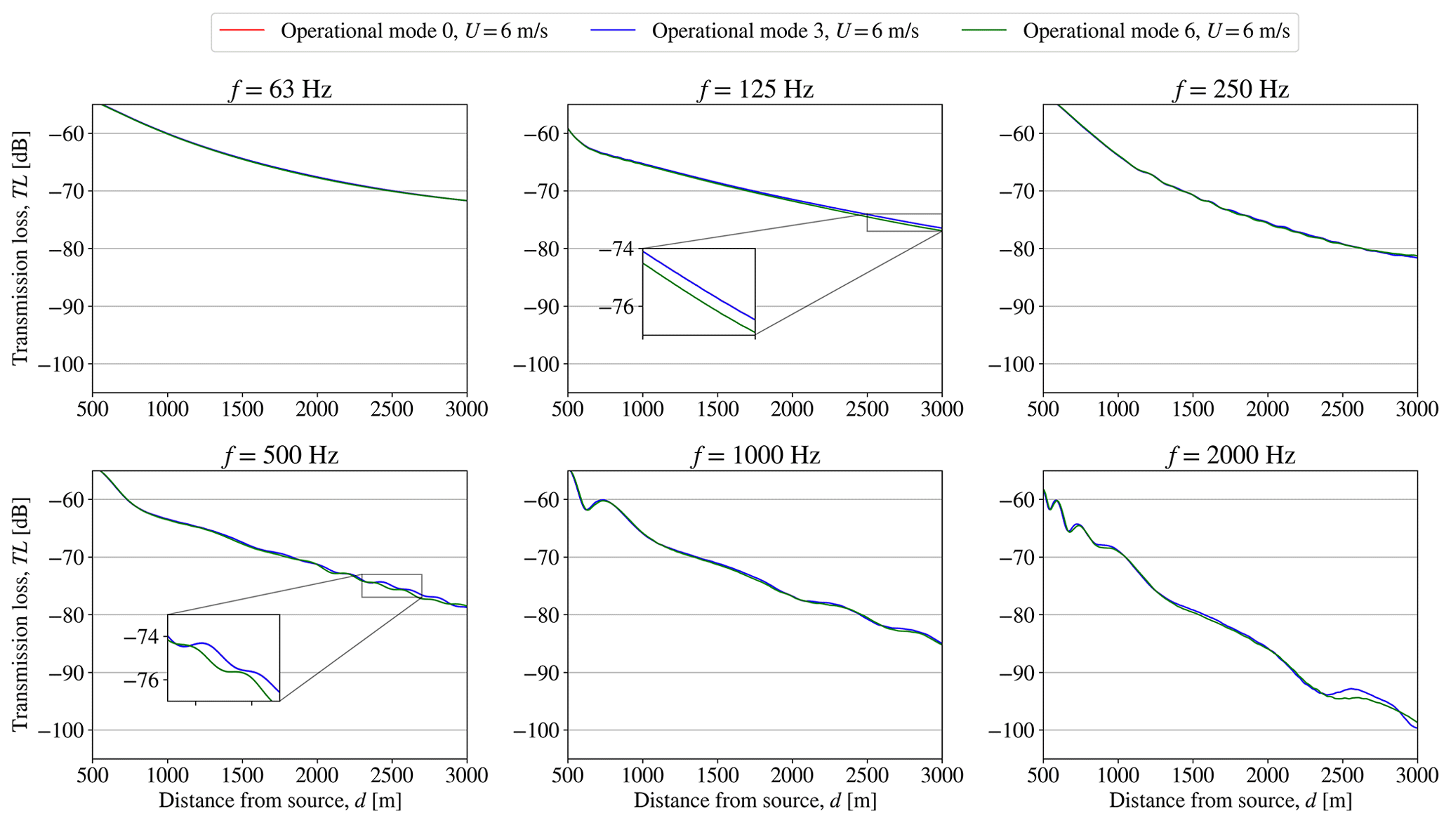
Figure A1Setup 1: CT sensitivity of WindSTAR obtained transmission loss, TL, from a single wind turbine subject to changing operational modes at each octave band frequency at a free field wind speed of U0=6 m s−1.
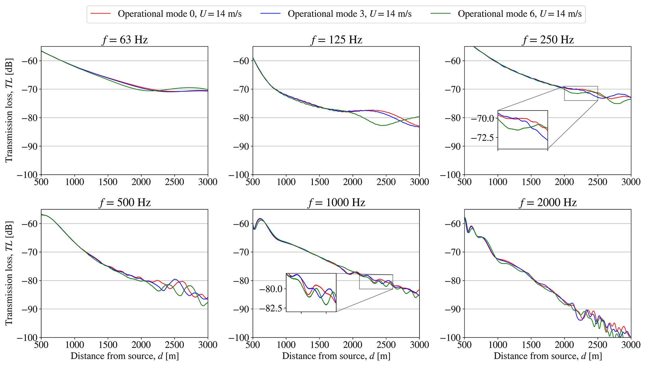
Figure A2Setup 1: CT sensitivity of WindSTAR obtained transmission loss, TL, from a single wind turbine subject to changing operational modes at each octave band frequency at a free field wind speed of U0=6 m s−1.
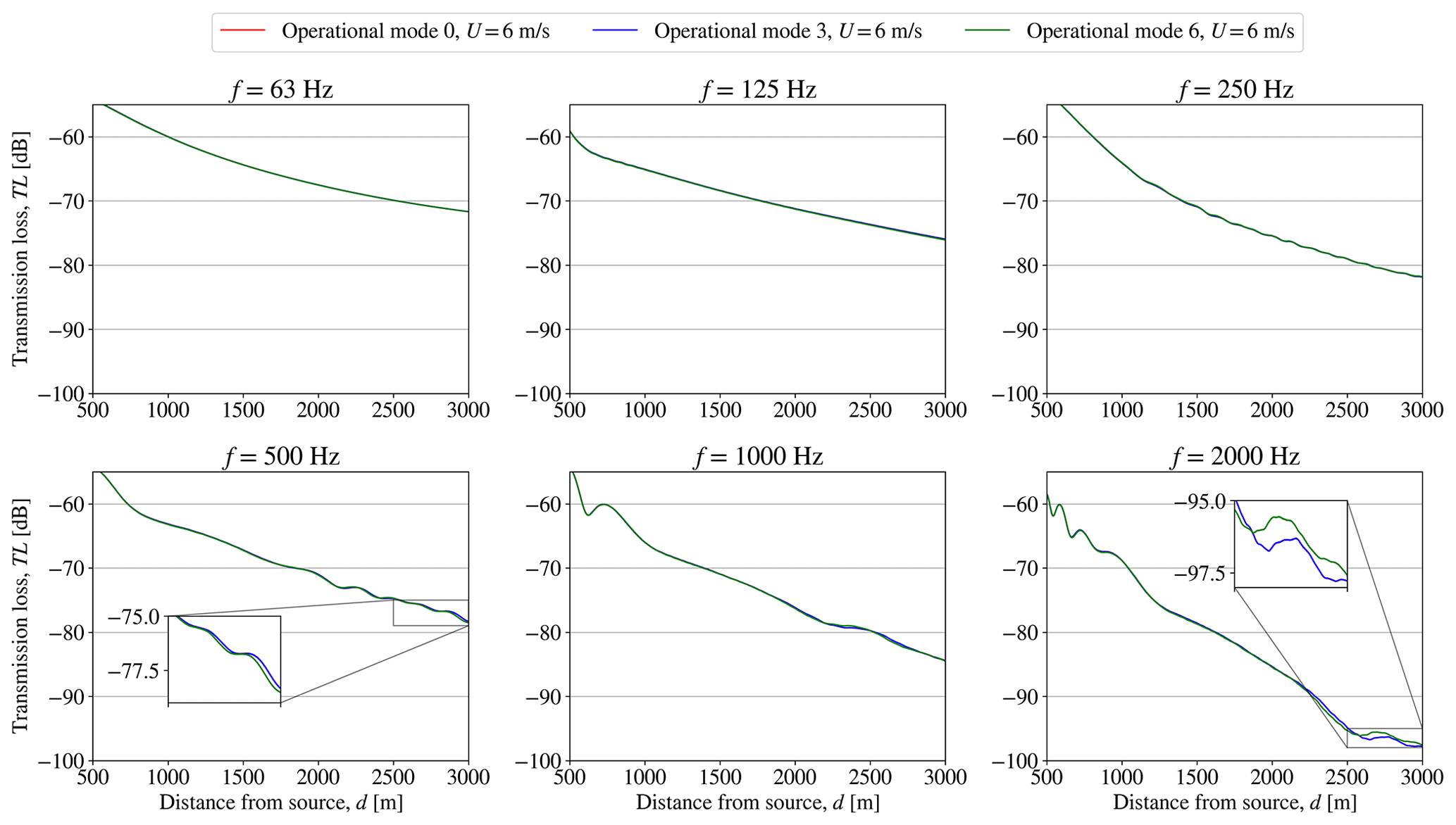
Figure A3Setup 2: CT sensitivity of WindSTAR obtained transmission loss, TL, from a single wind turbine positioned in the wake of a wind turbine subject to changing operational modes at each octave band frequency at a free field wind speed of U0=14 m s−1.

Figure A4Setup 2: CT sensitivity of WindSTAR obtained transmission loss, TL, from a single wind turbine positioned in the wake of a wind turbine subject to changing operational modes at each octave band frequency at a free field wind speed of U0=14 m s−1.
Topfarm is an open source optimization framework developed at the Technical University of Denmark. The implemented ISO 9613-2 standard model is open source, while the WindSTAR is proprietary software of the Technical University of Denmark.
Data will be made available upon request.
CMN: conceptualization, coupling of the ISO 9613-2 and WindSTAR sound propagation models to Topfarm, analysis of the sound propagation and optimization results, visualization, writing of the draft article. AF: conceptualization, analysis of the sound propagation results, supervision. PER: analysis of the optimization results, supervision. JF: conceptualization, supervision. All authors contributed to editing and finishing the article.
The contact author has declared that none of the authors has any competing interests.
Publisher's note: Copernicus Publications remains neutral with regard to jurisdictional claims in published maps and institutional affiliations.
The authors would like to thank Wen Zhong Shen at Yangzhou University for the valuable discussions regarding the optimization framework and the WindSTAR model. The authors would further like to acknowledge Jaime Liew from the Technical University of Denmark for his great help with the visualizations.
This paper was edited by Alessandro Bianchini and reviewed by Alessandro Fontanella and one anonymous referee.
Attenborough, K.: Acoustical Outdoor Impedance Models Surfaces, J. Sound Vibrat., 99, 521–544, https://doi.org/10.1016/0022-460X(85)90538-3, 1985. a
Barlas, E.: Development of an advanced noise propagation model for noise optimization in wind farm, DTU Wind Energy PhD, 80 pp., https://backend.orbit.dtu.dk/ws/files/146182107/Emre_Barlas_hele_afhandlingen.pdf (last access: 26 February 2023), 2017. a, b
Barlas, E., Zhu, W. J., Shen, W. Z., Dag, K. O., and Moriarty, P: Consistent modelling of wind turbine noise propagation from source to receptor, Appl. Acoust., 142, 3297–3310, https://doi.org/10.1121/1.5012747, 2017. a, b, c, d
Barlas, E., Wu, K. L., Zhu, W. J., Porté-Agel, F., and Shen, W. Z.: Variability of wind turbine noise over a diurnal cycle, Renew. Energy, 126, 791–800, https://doi.org/10.1016/j.renene.2018.03.086, 2018. a, b
Bastankah, M. and Porté-Agel, F.: A new analytical model for wind-turbine wakes, Renew. Energy, 70, 116–123, https://doi.org/10.1016/j.renene.2014.01.002, 2014. a
Bolin, K., Conrady, K., Karasalo, I., and Sjöblom, A.: An investigation of the influence of the refractive shadow zone on wind turbine noise, J. Acoust. Soc. Am., 148, EL166–EL171, https://doi.org/10.1121/10.0001589, 2020. a, b, c
Cao, J., Nyborg, C. M., Feng, J., Hansen, K. S., Bertagnolio, F., Fischer, A., Sørensen, T., and Shen, W. Z.: A new multi-fidelity flow-acoustics simulation framework for wind farm application, Renew. Sustain. Energ. Rev., 156, 111939, https://doi.org/10.1016/j.rser.2021.111939, 2022. a, b, c
Cao, J. F., Zhu, W. J., Shen, W. Z., Sørensen, J. N., and Sun, Z. Y.: Optimizing wind energy conversion efficiency with respect to noise: A study on multi-criteria wind farm layout design, Renew. Energy, 159, 468–485, https://doi.org/10.1016/j.renene.2020.05.084, 2020. a
Cotté, B.: Extended source models for wind turbine noise propagation, J. Acoust. Soc. Am., 145, 1363–1371, https://doi.org/10.1121/1.5093307, 2019. a
DS: International Standard 1993, ISO 9613-1: Acoustics – Attenuation of sound propagation outdoors – Part 1: Calculation of the absorption of sound by the atmosphere, Danish Standards Foundation, 1993. a
DS: International Standard 1997, ISO 9613-2: Acoustics – Attenuation of sound during propagation outdoors, Part 2: General method of calculation, Danish Standards Foundation, 1997. a, b, c
Evans, T. and Cooper, J.: Influence of wind direction on noise emission and propagation from wind turbines, Proceedings of Acoustics – Fremantle, https://www.acoustics.asn.au/conference_proceedings/AAS2012/papers/p139.pdf (last access: 26 February 2023), 2012. a
Feng, J. and Shen, W. Z.: Solving the wind farm layout optimization problem using random search algorithm, Renew. Energy, 78, 182–192, https://doi.org/10.1016/j.renene.2015.01.005, 2015. a, b
Feng, J. and Shen, W. Z.: Design optimization of offshore wind farms with multiple types of wind turbines, Appl. Energy, 205, 1283–1297, https://doi.org/10.1016/j.apenergy.2017.08.107, 2017. a, b, c
Gilbert, K. E. and Di, X.: A fast Green's function method for one-way sound propagation in the atmosphere, J. Acoust. Soc. Am., 94, 2343–2352, https://doi.org/10.1121/1.407454, 1993. a
Gilbert, K. E. and White, M. J.: Application Of The Parabolic Equation To Sound Propagation In A Refracting Atmosphere, J. Acoust. Soc. Am., 85, 630–637, https://doi.org/10.1121/1.397587, 1989. a
Gilbert, K. E., Raspet, R., and Di, X.: Calculation of turbulence effects in an upward-refracting atmosphere, J. Acoust. Soc. Am., 87, 2428–2437, https://doi.org/10.1121/1.399088, 1990. a
Gray, J. S., Hwang, J. T., Martins, J. R. R. A., Moore, K. T., and Naylor, B. A.: OpenMDAO: An open-source framework for multidisciplinary design, analysis, and optimization, Struct. Multidisciplin. Optimiz., 59, 1075–1104, https://doi.org/10.1007/s00158-019-02211-z, 2019. a
Jimenez, A., Crespo, A., Migoya, E., and Garcia, J.: Advances in large-eddy simulation of a wind turbine wake, J. Phys.: Conf. Ser., 75, 012041, https://doi.org/10.1088/1742-6596/75/1/012041, 2007. a
Lee, S., Lee, D., and Honhoff, S.: Prediction of far-field wind turbine noise propagation with parabolic equation, J. Acoust. Soc. Am., 140, 767–778, https://doi.org/10.1121/1.4958996, 2016. a
Martins, J. and Ning, A.: Engineering Design Optimization, Cambridge University Press, Cambridge, https://doi.org/10.1017/9781108980647, 2021. a, b, c
Michaud, D., Feder, K., Keith, S., Voicescu, Sonia, A., Marro, L., Than, J., Guay, M., Denning, A., McGuire, D., Bower, T., Lavigne, E. Murray, B. J., Weiss, S. K., and van den Berg, F.: Exposure to wind turbine noise: Perceptual responses and reported health effects, J. Acoust. Soc. Am., 139, 1443–1445, https://doi.org/10.1121/1.4942391, 2016. a
Mittal, P., Mitra, K., and Kulkarni, K.: Optimizing the number and locations of turbines in a wind farm addressing energy-noise trade-off: A hybrid approach, Energ. Convers. Manage., 132, 147–160, https://doi.org/10.1016/j.enconman.2016.11.014, 2017. a
Nieuwenhuizen, E. and Köhl, M.: Differences in noise regulations for wind turbines in four European countries, Euronoise, 333–338, ISSN 2226-5147, 2015. a, b, c
Nyborg, C. M.: Validation and application of advanced sound propagation modeling for optimization of wind farms, PhD thesis), DTU, https://doi.org/10.11581/dtu.00000247, 2022. a
Nyborg, C. M., Fischer, A., Thysell, E., Feng, J., Søndergaard, L. S., Sørensen, T., Hansen, T. R., Hansen, K. S., and Bertagnolio, F.: Propagation of wind turbine noise: measurements and model evaluation, J. Phys.: Conf. Ser., 2265, 032041, https://doi.org/10.1088/1742-6596/2265/3/032041, 2022. a, b
Oerlemans, S., Sijtsma, P., and Lopez, B. M.: Location and quantification of noise sources on a wind turbine, J. Sound Vibrat., 299, 869–883, 2007. a
Pedersen, M. M., van der Laan, P., Friis-Møller, M., Rinker, J., and Réthoré, P.: DTUWindEnergy/PyWake: PyWake, Zenodo [code], https://doi.org/10.5281/zenodo.2562662, 2019. a, b
Pedersen, M. M., Friis-Møller, M., Réthoré, P., Rinker, J., and Riva, R.: DTUWindEnergy/TopFarm2: v2.2.3, Zenodo [code], https://doi.org/10.5281/zenodo.4876330, 2021. a, b
Pollini, N.: Topology optimization of wind farm layouts, J. Renew. Energ., 195, 1015–1027, https://doi.org/10.1016/j.renene.2022.06.019, 2022. a
Poulsen, A., Raaschou-Nielsen, O., Peña, A., Hahmann, A. N., Nordsborg, R. B., Ketzel, M., Brandt, J., and Sørensen, M.: Short-term nighttime wind turbine noise and cardiovascular events: A nationwide case-crossover study from Denmark, Environ. Int., 114, 160–166, https://doi.org/10.1016/j.envint.2018.02.030, 2018. a
Poulsen, A., Raaschou-Nielsen, O., Peña, A., Hahmann, A. N., Nordsborg, R. B., Ketzel, M., Brandt, J., and Sørensen, M.: Impact of long-term exposure to wind turbine noise on redemption of sleep medication and antidepressants: A nationwide cohort study, Environ. Health Perspect., 127, 1–9, https://doi.org/10.1289/EHP3909, 2019. a
Réthoré, P.-E., Fuglsang, P. , Larsen, G. C., Buhl, T., Larsen, T. J., and Madsen, H. A.: TOPFARM: Multi-fidelity optimization of wind farms, Wind Energy, 17, 042035, https://doi.org/10.1002/we.1667, 2020. a
Riva, R., Liew, J. Y., Friis-Møller, M., Dimitrov, N., Barlas, E., Réthoré, P.-E., and Berzonskis, A.: Wind farm layout optimization with load constraints using surrogate modelling, J. Phys.: Conf. Ser., 1618, 042035, https://doi.org/10.1088/1742-6596/1618/4/042035, 2014. a, b
Sack, R. A. and West, M.: A parabolic equation for sound propagation in two Dimensions over any smooth terrain profile: The Generalised Terrain Parabolic Equation (GT-PE), Appl. Acoust., 45, 113–129, 1995. a
Salomons, E.: Improved Green’s function parabolic equation method for atmospheric sound propagation, J. Acoust. Soc. Am., 104, 100–111, https://doi.org/10.1121/1.423260, 1998. a
Salomons, E. M.: Computational Atmospheric Acoustics, Springer Science + Business Media, B.V., https://doi.org/10.1007/978-94-010-0660-6, 2001. a, b, c, d
Shen, W. Z., Zhu, W. J., Barlas, E., and Li, Y.: Advanced flow and noise simulation method for wind farm assessment in complex terrain, Renew. Energy, 143, 1812–1825, 2019. a
Sorkhabi, S. Y. D., Romero, D. A., Yan, G. K., Gu, M. D., Moran, J., Morgenroth, M., and Amon, C. H.: The impact of land use constraints in multi-objective energy-noise wind farm layout optimization, Renew. Energy, 85, 359–370, https://doi.org/10.1016/j.renene.2015.06.026, 2016. a
Tingey, E. B. and Ning, A.: Trading off sound pressure level and average power production for wind farm layout optimization, Renew. Energy, 114, 547–555, https://doi.org/10.1016/j.renene.2017.07.057, 2017. a
van der Laan, M. P., Sørensen, N. N., Réthoré, P.-E., Mann, J., Kelly, M. C., Troldborg, N., Schepers, J. G., and Machefaux, E.: An improved k–ϵ model applied to a wind turbine wake in atmospheric turbulence, Wind Energy, 18, 889–907, https://doi.org/10.1002/we.1736, 2015. a
Wagner, S., Bareiß, R., and Guidati, G.: Wind turbine noise, EUR 16823, Springer, https://doi.org/10.1007/978-3-642-88710-9, 1996. a
West, M., Gilbert, K., and Sack, R. A.: A tutorial on the parabolic equation (PE) model used for long range sound propagation in the atmosphere, Appl. Acoust., 37, 31–49, https://doi.org/10.1016/0003-682X(92)90009-H, 1992. a
Wu, X., Hu, W., Huang, Q., Chen, C., Jacobson, M. Z., and Chen, Z.: Optimizing the layout of onshore wind farms to minimize noise, Appl. Energy, 267, 114896, https://doi.org/10.1016/j.apenergy.2020.114896, 2020. a