the Creative Commons Attribution 4.0 License.
the Creative Commons Attribution 4.0 License.
 | 22 Mar 2023
Actuator line model using simplified force calculation methods
Gonzalo Pablo Navarro Diaz
Alejandro Daniel Otero
Henrik Asmuth
Jens Nørkær Sørensen
Stefan Ivanell
To simulate transient wind turbine wake interaction problems using limited wind turbine data, two new variants of the actuator line technique are proposed in which the rotor blade forces are computed locally using generic load data. The proposed models, which are extensions of the actuator disk force models proposed by Navarro Diaz et al. (2019a) and Sørensen et al. (2020), only demand thrust and power coefficients and the tip speed ratio as input parameters. In the paper the analogy between the actuator disk model (ADM) and the actuator line model (ALM) is shown, and from this a simple methodology to implement local forces in the ALM without the need for knowledge of blade geometry and local airfoil data is derived. Two simplified variants of ALMs are proposed, an analytical one based on Sørensen et al. (2020) and a numerical one based on Navarro Diaz et al. (2019a). The proposed models are compared to the ADM using analogous data, as well as to the classical ALM based on blade element theory, which provides more detailed force distributions by using airfoil data. To evaluate the local force calculation, the analysis of a partial-wake interaction case between two wind turbines is carried out for a uniform laminar inflow and for a turbulent neutral atmospheric boundary layer inflow. The computations are performed using the large eddy simulation facility in Open Source Field Operation and Manipulation (OpenFOAM), including Simulator for Wind Farm Applications (SOWFA) libraries and the reference National Renewable Energy Laboratory (NREL) 5 MW wind turbine as the test case. In the single-turbine case, computed normal and tangential force distributions along the blade showed a very good agreement between the employed models. The two new ALMs exhibited the same distribution as the ALM based on geometry and airfoil data, with minor differences due to the particular tip correction needed in the ALM. For the challenging partially impacted wake case, both the analytical and the numerical approaches manage to correctly capture the force distribution at the different regions of the rotor area, with, however, a consistent overestimation of the normal force outside the wake and an underestimation inside the wake. The analytical approach shows a slightly better performance in wake impact cases compared to the numerical one. As expected, the ALMs gave a much more detailed prediction of the higher-frequency power output fluctuations than the ADM. These promising findings open the possibility to simulate commercial wind farms in transient inflows using the ALM without having to get access to actual wind turbine and airfoil data, which in most cases are restricted due to confidentiality.
- Article
(5796 KB) - Full-text XML
- BibTeX
- EndNote


In recent years, large eddy simulation (LES) of wind farms has become feasible due to the emergence of fast computers and the development of the actuator disk and line methods. Hence, today it is possible to capture the interaction of the wind flow between the wind turbines (WTs) and transient problems in the atmospheric boundary layer (ABL), including the variation in the mean wind and turbulence associated with the diurnal cycle (Abkar et al., 2016; Englberger and Dörnbrack, 2018), as well as ramps and changes in wind directions (Arthur et al., 2020; Stieren et al., 2021). Using LES techniques facilitate the understanding of the interaction between the ABL and the WTs in wind farms and make it possible to capture the variation in the structure of WT wakes and their effects on loads and power losses (Abkar et al., 2016; Porté-Agel et al., 2020). The study of the variation in WT power output for different inflow conditions is also important for determining the necessary fill-in power needed to follow a signal from the grid operator (Bossuyt et al., 2016). The well-known excessive computational cost that constrains the usability of LES based on Navier–Stokes equation implementations on central processing units (CPUs) has been drastically reduced due to the new implementations in graphics processing units (GPUs), for example using the Lattice Boltzmann method (Asmuth et al., 2022), making LES studies accessible for large wind farms and for long time periods. One of the challenges when simulating transient WT wake problems is the need to access detailed wind turbine data, such as the operating setting and the geometric and aerodynamic characteristics of the blade. This information, which usually is subject to confidentiality, is needed for the calculation of blade forces using the classical blade element (BE) theory, which is an inherent part of the actuator line model (ALM) (Sørensen and Shen, 2002). In the ALM, the forces are distributed over rotating lines representing the effect of the blades on the flow, which enables transient simulations of the flow in wind farms. In most cases, however, it is only possible to get access to generic open WT data, i.e., rotor radius (R) and thrust and power coefficients (CT and CP) as a function of tip speed ratio (λ).
This kind of input data is normally sufficient for performing computations using the actuator disk method (ADM), as the loading in this method is spread over the surface (the disk) representing the swept rotor area (Navarro Diaz et al., 2019a). However, distributing the forces on a disk instead of on rotating lines does not capture correctly the physics of the vortex pattern in the wake. A LES study by Martinez et al. (2012) showed that the root and tip vortices produced by the blades in the ALM are not developed in the ADM, which only generates a shear layer surrounding the wake. A similar LES comparison was carried out by Stevens et al. (2018), who found differences between the two models up to three rotor diameters downstream. Furthermore, Marjanovic et al. (2017) carried out ALM computations in realistic ABL flows and found that the ALM generates distinct tip and root vortices that keep their coherence as helical tubes at least one diameter downstream of the rotor plane. Seen in the light of the possibility of using generic load distributions in the ADM and the advantage of the ALM to capture correctly transient flows, we here explore the possibility of combining the two methods by implementing a generic load model in the ALM.
In order to develop a generic load model for the ALM, we exploit the recent achievements of the ADM to improve the calculation of forces from local information of the flow over the disk while keeping the input parameters at a minimum. Using local flow properties allows the model to have a better performance in complex inflow conditions, such as ABL profiles in flat or complex terrain, or for rotors subject to partial- or total-wake impact. The first example is the analytical ADM developed by Sørensen et al. (2020), in which analytical expressions specify the radial distribution for both the normal and tangential components of the blade body force. This formulation assumes that the rotor disk is subject to a constant circulation corrected for tip and root effects and has the advantage that it for a given wind turbine size only demands the thrust and power coefficients as a function of tip speed ratio as input. The calculation of the forces is done locally; hence, the model is capable of handling non-uniform velocity fields over the rotor, for example, produced by the vertical velocity profile of the ABL or the impact of wakes from surrounding wind turbines. The model was recently extended to determine the annual energy production in small and large wind farms by van der Laan et al. (2022). Another example is the model by Navarro Diaz et al. (2019b), where the local adaptation of the ADM is obtained by using a numerical approach. This procedure consists of deriving two pre-calibrated tables for a wide range of WT operating conditions, which subsequently are used for the calculation of the local forces on the rotor plane. The analytical and numerical approaches perform very well for velocities below the rated power, as the authors explain in their original papers (Sørensen et al., 2020; Navarro Diaz et al., 2019a). For velocities above the rated power, however, the two approaches still need some improvements.
The novelty of the present work is the development of two new ALMs which, based on the earlier developed analytical and numerical ADM approaches, are capable of simulating transient WT wake flows without the need of blade geometry and local airfoil data. The models are verified and compared for a wide range of flow cases, covering both uniform inflow and partial-wake impact subject to non-turbulent and turbulent ambient conditions in the ABL. Furthermore, the capabilities of the ALMs to improve the time-dependent response of the turbine are studied.
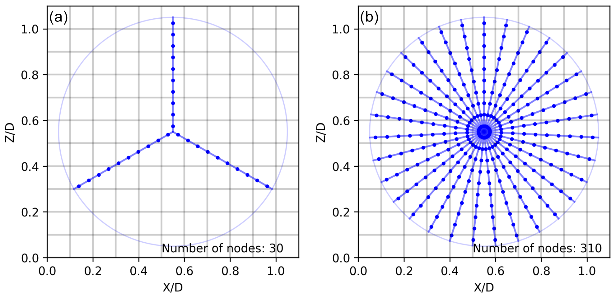
Figure 1Example of the node distribution strategy on lines for the ALM (a) and the ADM (b). In this example, a coarse mesh of 10 cells along the diameter is taken to make the node distribution clearer for the reader.
This work is organized as follows. First, in Sect. 2.1 the similarities and differences between the ADM and the ALM concepts are described, followed by the formulation for the local force calculation based on three different approaches: one requiring detailed airfoil data as input (Sect. 2.1.1) and the two others only requiring the thrust and power coefficients as input parameters (Sect. 2.1.2 and 2.1.3). The Open Source Field Operation and Manipulation (OpenFOAM) software configuration is described in Sect. 2.2, followed by the description of the National Renewable Energy Laboratory (NREL) 5 MW reference WT (Sect. 2.3). The models are tested in Sect. 3 for different inflow conditions: first, for a uniform non-turbulent inflow with a single-WT layout (Sect. 3.1.1) and a layout with two non-aligned WTs (Sect. 3.1.2), and second, for a turbulent ABL inflow with two non-aligned WTs (Sect. 3.2). Finally, in Sect. 4 conclusions are presented.
2.1 Force modeling
The basic idea behind the actuator disk is to replace the three-dimensional geometry of the blades by equivalent forces acting on the flow. This strategy allows us to save computational costs, avoiding the need to resolve the blade boundary layer and replacing the otherwise boundary-fitted mesh around the solid blade surface by a coarse mesh with distributed volumetric forces (Sanderse et al., 2011).
Figure 1 depicts the two most common actuator WT models. First, in the actuator line model, ALM, the WT is represented by rotating lines moving with a rotational speed, ω. In this model, the number of lines, nl, is equal to the number of blades, B. These lines are discretized in nodes, i, which represent the contribution of a radial fragment of the blade, Δb, where the normal, Fn,i, and tangential, Fθ,i, forces are calculated. The separation between the nodes, Δb, is recommended to be dependent on the horizontal cell size, Δx, assuming Δb=0.5Δx (Asmuth et al., 2020). In the actuator disk model, ADM, the forces are instead distributed over the entire rotor swept area. To make an analogy to the ALM, in this work the disk is represented by multiple non-rotating artificial lines (Nathan et al., 2015; Martinez et al., 2012). The idea behind the proposed technique is that there exists a full correspondence between the ADM and the ALM such that the advantage of using generic WT data in the ADM also can be exploited in the ALM. To ensure that there is at least one node in each cell at the tip of the ADM, the number of lines, nl, in the ADM is calculated as
where R is the radius of the rotor blade. In the ADM, using the described method, for each time step in the solution procedure the forces are computed and distributed on all nodes on the entire disk surface. In contrast to this, in the ALM only the nodes representing the blades are active as carriers of the forces. Due to the rotation of the blades, the active points move as a function of time. Using a time step,
ensures that the blade tip does not translate faster than one cell per time step (see Fig. 1). One important characteristic to mention is the number of nodes needed in each model, since this quantity has a direct relation with the computational cost of the model for each time step. Using the analogy between the ADM and the ALM presented here, the ADM seems to demand 10 times more nodes than the ALM. However, in reality significantly fewer points are needed in an actual computation using the ADM, and the ALM will generally be more computationally demanding due to the limitation of the time step. In both models, ALM and ADM, the normal (ΔFn,i) and tangential (ΔFθ,i) forces per area unit are calculated based on the force's calculation method adopted and are then concentrated (Fn,i and Fθ,i) for each node i as
where ΔAi is the disk area corresponding to each node, obtained as
and ri the local radial position from the center of the turbine.
It should be noted that, in this work, the only difference between the ALM and the ADM is the number of lines nl and the tip and root corrections adopted. To express the normal and tangential forces per length unit along the blade (fn,i and fθ,i), node forces are divided by the blade element length Δb as
Finally, the total thrust, T, and power, P, are obtained as
To avoid numerical instability, the normal and tangential forces in each node are then distributed by means of a three-dimensional Gaussian function using a regularization kernel (ηcell) (Porté-Agel et al., 2011) in neighboring cells:
where d is the distance between the node and the center of the cell and ε is the smearing factor, commonly fixed as ε=2Δx (Howland et al., 2016). To take into account this force distribution in non-uniform meshes, the volume of the cell (Vcell) is considered in the force Eqs. (10) and (11).
WTs in wind farms are affected by non-uniform velocity fields due to the ABL flow, the influence of the topography and the upstream WT wakes. This creates the necessity of a local force calculation in the ALM and the ADM in order for the model to give a better and more realistic response to this complex velocity field. The local calculation of ΔFn,i and ΔFθ,i depends on the available information of the WT. If the operating setting and the geometrical and aerodynamic characteristics of the blade are available, the classic BE theory can be used. On the other hand, if only generic WT data, i.e., R, CT, CP and λ, are available, then the forces can be calculated by means of the analytical (Sørensen et al., 2020) or numerical (Navarro Diaz et al., 2019b) approach.
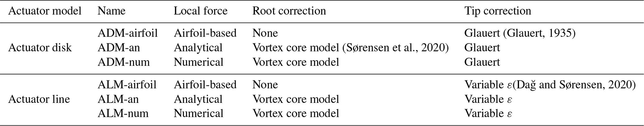
Based on the two types of actuator models (ALM and ADM) and the three approaches to calculate the local forces (BE, analytical and numerical), six models in total are implemented. Table 1 shows an overview of the different models, specifying the tip and root corrections, as well as the naming convention. In the following, the calculation procedure of the local forces is explained for the various models.
(Glauert, 1935)(Sørensen et al., 2020)(Dağ and Sørensen, 2020)Table 1Actuator disk and actuator line models employed in this work, describing the differences in the local force calculation and the chosen tip and root corrections.
2.1.1 Airfoil-based forces
The first ADM combining BE theory with computational fluid dynamics (CFD) is from Sørensen and Myken (1992) and Sørensen and Kock (1995). This model was later extended to the ALM and used in combination with LES (Sørensen and Shen, 2002; Nathan et al., 2018; Sørensen et al., 2015; Nathan et al., 2017; Asmuth et al., 2020). Later developments combining LES with the ADM are, for example, from Porté-Agel et al. (2011) and van der Laan et al. (2015). Using a BE approach requires detailed knowledge regarding the WT operating setting, as well as the geometrical and aerodynamic characteristics of the rotor blade.
First, the general operating regime of the WT needs to be obtained, which is related to the reference velocity Uref. Knowing Uref the pitch angle Θp and rotational speed ω can be extracted from the WT characteristics. In cases when Uref is unknown, a torque controller is the standard method that provides the rotational speed of the turbine. In cases when a torque controller is not possible to implement due to the lack of blade information, a simple calibration table can be used (van der Laan et al., 2015) by creating a calibration table with the relation between the average velocity over the disk (〈Ud〉) and the Uref. This approach can not account for inertial affects on the rotational speed of the rotor.
Once the operating regime is determined, the forces are calculated for each node, as described in the following. First, the relative velocity Urel in the blade element is obtained as
where Un and Uθ are the local normal and tangential velocities, respectively. It is important to clarify that the local velocity vector is calculated by linear interpolation with the eight closest cells to the node position. The angle between Urel and the rotor plane is calculated as
The local angle of attack is determined as , where β is the sum of the flow angle Θp and the “twist” of the blade in the local radial position r. Then, the lift, ΔFL, and drag, ΔFD, forces per unit area are obtained as
where the airfoil information needed includes the chord length c, the lift and drag coefficients CL and CD, and the lift and drag unit vectors eL and eD. In these equations ρ is the air density, B is the number of blades (B=3) and ℱtip and ℱroot are the tip and root corrections, respectively. The corrections used in this work are separately explained in Sect. 2.1.4. Finally, the normal and tangential components per unit of area are obtained as
2.1.2 Analytical force distribution
The analytical local force calculation was originally proposed by Sørensen et al. (2020) to be used in the ADM, analyzing the performance of this new model for both a single WT and two aligned WTs in an ABL inflow. Also, this model was validated in Sørensen and Andersen (2020) for four different WTs operating under a wide range of conditions. The main advantage of this analytical ADM is that the expressions only depend on global parameters, such as rotor radius R, tip speed ratio λ, and thrust coefficient CT.
In this work, the implementation of this model is done following the next steps. First, in the cases where Uref is not fixed and needs to be estimated, the average velocity over the rotor disk 〈Ud〉 is determined and the WT operating regime is obtained by determining Uref using the following analytical formulation,
which is based on the same relation present in Eq. (26). Due to the fact that commercial WTs, as well as the reference turbine used in this work, have a CT curve depending on Uref, an iterative process of calculating Uref is needed. Next, the tip speed ratio, λ, is calculated as
This model formulation requires the tip ℱtip and root ℱroot corrections for all the radial positions. Thus the dimensionless reference circulation, q0, is calculated as
where a1 and a2 are the result of integrating ℱtip and ℱroot along the blade as
where is the non-dimensional radial distance, depending on the local radius r. Finally, the local normal, ΔFn,i, and tangential, ΔFθ,i, forces over the disk area for each node i are calculated as
In these two equations U∞ is the upstream unperturbed velocity for force calculation, which is defined in the analytical ADM as
where Ud,i is the local disk velocity at the node.
2.1.3 Numerical force distribution
A local calculation of forces using a numerical approach was originally proposed by Navarro Diaz et al. (2019b) to improve the performance of the ADM for complex flows in wind farm simulations. This methodology was also used in four ADMs with increasing levels of complexity (Navarro Diaz et al., 2019a), proving that the local calculation improves the solution for wake interaction cases. The model has shown a satisfactory performance for capacity factor estimation in an onshore wind farm (Navarro Diaz et al., 2021).
In the formulation from the original publication, with no tip and root corrections included, the non-corrected normal and tangential forces per unit of area are calculated as
In this numerical adaptation approach, U∞ is the upstream velocity which, for uniform incoming flows, can be assumed equivalent to Uref.
In order to apply the tip ℱtip and root ℱroot corrections and conserve the total thrust and power output, the normal ΔFn and tangential ΔFθ forces per unit of area are scaled as
where b1 and b2 are scale factors for the normal and tangential forces, respectively, obtained as
In the cases when the upstream reference wind velocity Uref, which defines the turbine setting given by CP, CT and ω, is unknown, it needs to be estimated from the average wind velocity over the disk area 〈Ud〉. Note that the wind velocity at a certain location on the disk Ud,i does not necessarily have to coincide with 〈Ud〉, especially under complex flow patterns. This Ud,i is the velocity that defines the local effect of the actuator disk on the flow. So, given a particular turbine setting defined by Uref, at each location there will be a relation between Ud,i and a corresponding unperturbed upstream wind velocity U∞ which will determine the local forces. This differentiation between the wind velocity adopted in the WT setting Uref and the unperturbed wind velocity used to calculate the ADM forces U∞, introduced by Navarro Diaz et al. (2019a), provides the ADM with the capability to adapt the forces in areas that work under off-design conditions.
The numerical ADM implementation requires a calibration process where the turbine is operated to face different uniform inflow cases. This process allows us to establish a relationship between local velocities at the ADM and the corresponding unperturbed velocities: firstly, the relation between 〈Ud〉 and Uref (defining the respective CT and CP); and secondly for each Uref configuration, the relation between Ud,i and ΔFn,i and ΔFθ,i. These relations are expressed in Tables 2 and 3. To construct Table 2, a simulation is run for each inflow velocity U∞ in the WT operating range, making the ADM impose the forces ΔFn,i and ΔFθ,i on the fluid according to the thrust and power at that given velocity. In each of these simulations, the turbine stands alone in the middle of the domain, following the same detailed specifications that are addressed in Sect. 2.2 for the mesh sensitivity analysis case. Thus, the resulting average velocity 〈Ud〉 is measured, disclosing the relation between 〈Ud〉 and the reference velocity Uref assumed equal to the U∞ in that case, in a procedure similar to that proposed by van der Laan et al. (2015). The second and third columns of Table 2 come from the WT manufacturer specifications.
Table 2Example of the table defining the relation between the average velocity on the disk (〈Ud〉) and the reference operational velocity of the WT (Uref), with the corresponding coefficients CT and CP. The values were calculated using the ADM-airfoil and corresponds to inflow velocities below and above rated velocity (Uref=11.4 m s−1) for the NREL 5 MW.
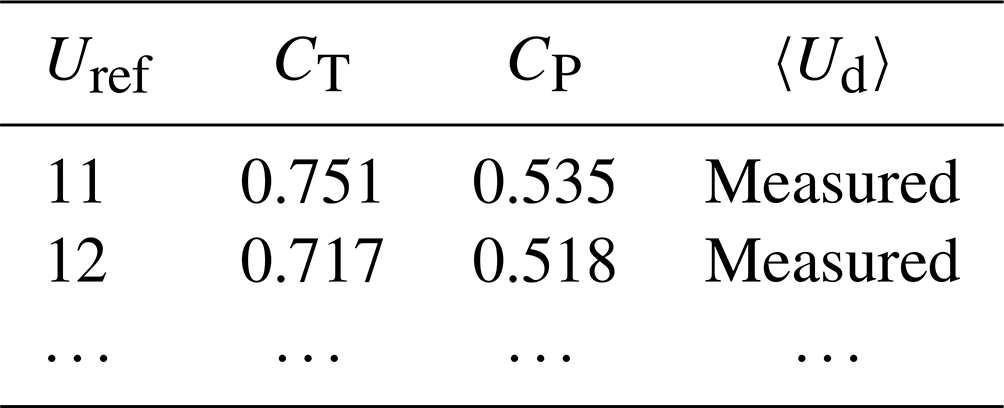
Table 3Example of the calibration table to obtain the relations between the local velocity on the node (Ud,i) and the unperturbed velocity (U∞) used for the local force calculation on the node.
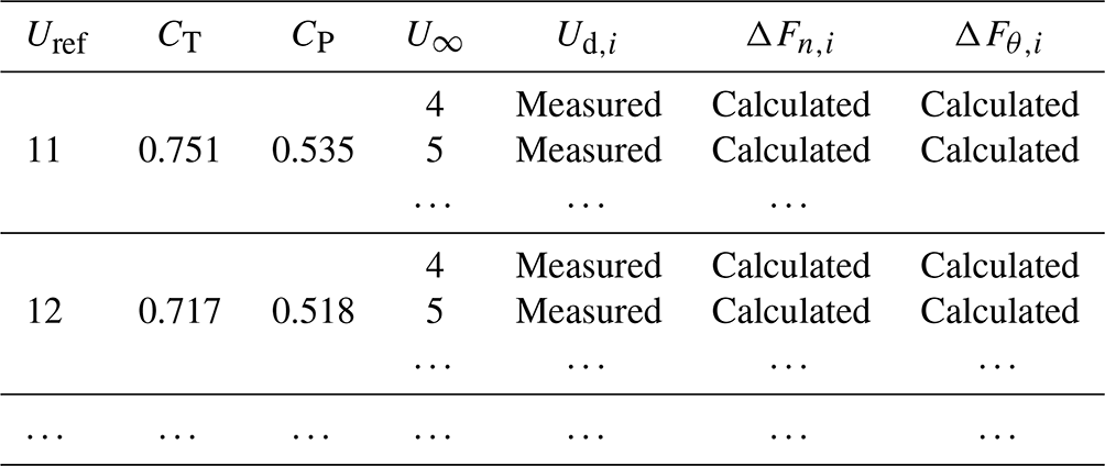
To construct Table 3, for each CT, CP and λ in accordance to a reference velocity Uref in the WT operating range, different inflow velocities U∞ are imposed in each simulation along with the resulting ADM forces, saving the local velocity Ud,i and forces ΔFn,i and ΔFθ,i for each discrete radial position ri (columns 5 to 7 of Table 3). Compared to the procedure followed in Navarro Diaz et al. (2019a) where there was no tip and root correction, the values of ΔFn,i and ΔFθ,i are needed in this case as they include these corrections.
Afterwards, in each time step of the wind farm simulation, the ADM implementation takes the average velocity over the disk, 〈Ud〉, and uses Table 2 to interpolate Uref and obtain the CT and CP values. Then, in each ADM node, it takes the velocity Ud,i and by means of Table 3 interpolates the corresponding ΔFn and ΔFθ.
2.1.4 Tip and root corrections
The tip and root corrections adopted in each ADM and ALM are summarized in Table 1. In the case of the ADM, this model assumes that the flow is azimuthally uniform in the rotor plane and thus requires a tip loss correction to take into account the effect of a finite number of blades. For this work, the Glauert tip loss correction (Glauert, 1935) is used, following the recommendation by Sørensen and Andersen (2020). This correction was developed from the study of Prandtl (Zhong et al., 2019) and can be expressed as
In the ALM there is also the need of introducing another type of correction to address the problem of the thickness of the shed vortices in the ALM produced by smearing the blade forces into the CFD domain. This has lately been discussed and solved in the works by Jha and Schmitz (2018) and Dağ and Sørensen (2020). The correction proposed by Jha and Schmitz (2018) is the most suitable for this work due to the small amount of blade information needed in the formulation. This correction consists of making ϵ dependent on the local radial position, with restricting it to ϵ=1 at the tip. The only limitation on this correction is the need of the chord length values at each airfoil section. To overcome this, a simpler ϵ variation is proposed, setting ϵ=2 from the root up to the middle of the blade and then reducing it linearly to ϵ=1 at the tip.
The root correction ℱroot is based on a vortex core model, used in the original work of the ADM-an (Sørensen et al., 2020), to account for the inner non-lifting part of the rotor. This part of the blade is only correctly described in the ADM-airfoil and the ALM-airfoil, avoiding the need of root correction. For the rest of the models, the correction is expressed as
where b=4 and a=2.335 are two coefficients whose values are adopted from the original analytical ADM paper. is the vortex core, defined as the non-dimensional distance from the root to the point where the lift force becomes active. This distance depends on the blade, and, for the reference turbine used in this work, a value gives the best fit compared to the ADM based on airfoil data.
2.2 Numerical setup
In this work the open-source software OpenFOAM (version 2.3.1) is used in conjunction with the Simulator for Wind Farm Applications (SOWFA) libraries (Churchfield et al., 2012b) developed by the NREL. LES is chosen in order to capture the transient flow solution using the ALM and compare it with the ADM. Both sets of turbine models, ALM and ADM, have been re-implemented in the comparison with the original code provided in SOWFA following the abovementioned developments. This implementation strategy allows the ALM and the ADM to have the same base code, meaning that the node distribution and tip and root corrections are the only sources of differences. A simple one-equation eddy viscosity approach is employed as a sub-grid-scale (SGS) model (Yoshizawa, 1986). Two flow situations, uniform and ABL inflows, are considered to analyze the model performance for different ambient turbulence conditions.
Both single-turbine and double-turbine interaction configurations are performed for the uniform inflow case. In the single-turbine case, two domains are used. For the mesh sensitivity analysis a cubic domain configuration with dimensions of 6 D on each side is specified, with the turbine located at the center of the domain. For the model and wake comparison a longer domain in the streamwise direction is used, consisting of a 10 D long domain located downstream of the turbine position. The mesh consists of cubic cells, having different refinement zones near the turbine in order to achieve the desired resolution in the rotor disk. The details of the refinement zones can be seen in Fig. 2. In the double-turbine interaction case, the turbines (WT1 upstream and WT2 downstream) are 5 D apart in the streamwise direction and 0.5 D in the spanwise direction. This layout generates a half-wake impact on the rotor plane of the downstream turbine, WT2, representing one of the most complex flow conditions that a turbine model can face. This layout is similar to the one used in Navarro Diaz et al. (2019a). The turbine positions, together with the mesh refinement zones, can be seen in Fig. 2. The simulation is performed in a time span of 660 s, with the last 60 s, corresponding to 9.15 blade revolutions, sampled for analysis.

Figure 2Horizontal domain size and cell size in the mesh refinement zones for the non-turbulent inflow cases: (a) and (b) for the mesh sensitivity analysis and (c) for the wake analysis with a single turbine. In (d) the domain for the double-WT layouts is shown. The only difference between the single-turbine cases is the cell sizes.
For the ABL inflow, a neutral stratified condition is simulated, and the turbulent solution is achieved by means of a precursor simulation with periodic boundary conditions. In this stage, a horizontal domain extension of and a total height of 1 km are chosen (Churchfield et al., 2012b). In this domain, a capping inversion starting from 700 m above the ground is fixed. The inclusion of the capping inversion and the domain dimensions follow the recommendation by Churchfield et al. (2012b), who remark that the capping inversion in neutral conditions helps to slow the vertical growth of the boundary layer with time. In SOWFA, a desired horizontal average velocity and direction at hub height can be forced in every time step by adjusting the magnitude and direction of the driving pressure gradient. Because this is an idealized study case, the terrain is flat and the Coriolis force is not included in the simulations. Due to the fact that the Coriolis force is neglected, the average velocity vector does not veer with height, and, if the velocity direction is fixed at 270∘, very large streamwise-elongated coherent structures would only have 3 km to travel before entering again into the domain. This situation is problematic in the solution when periodic boundary conditions are chosen, as also addressed by Munters et al. (2016). In order to avoid this problem, a direction which is not aligned with the domain sides is forced, giving more distance for the coherent structures to travel before entering from the same inlet face position. This strategy was also used in SOWFA by Wang et al. (2018). If a maximum coherent structure spanwise dimension (dy) similar to the ABL height ( m) is assumed, the inclination angle can be calculated as ∘. With this inclination, the structures travel through a total distance of lxcos (γ)=12.46 km (more than 4 times lx). This configuration can be seen in Fig. 3 with the total distance remarked as a continuous line in the left image. In the precursor, the cells in the mesh have a horizontal dimension of 16 m (approximately ) and a vertical dimension that grows with height, starting with 2.5 m and finishing with 60 m at the top. The roughness length (z0) is determined according to the desired turbulence intensity (TI) at hub height, defined as
where TKE is the turbulent kinetic energy also at hub height. The relation between this TI and the standard one obtained with a cup anemometer for a neutral ABL is (van der Laan et al., 2015). In this work, z0=0.1 m is adopted, corresponding to TI=7.8 % (TIcup=9.75 %), which is similar to the one used in the double-WT interaction study on an onshore wind farm from van der Laan et al. (2015). The precursor is computed for 5 h (18 000 s) to obtain a quasi-steady state (Churchfield et al., 2012a). In the next 1 h and 10 min the values at the corresponding inlet faces are recorded for each time step in order to use them for the farm.
In the farm stage, the mesh is refined in the wake zone and near the turbines. Figure 3 shows more details of the domain size and mesh refinement zones in horizontal and vertical planes. It is important to remark that, when the flow enters the refinement region of , it travels a distance of 10.74 D (1353 m) before reaching the first turbine, a distance that is long enough to develop the eddy structures in the new refined mesh. The cylindrical zone around each turbine is refined to with the objective to follow the mesh sensitivity study recommendation near the rotor plane (Sect. 3.1.1) without developing new eddy structures.
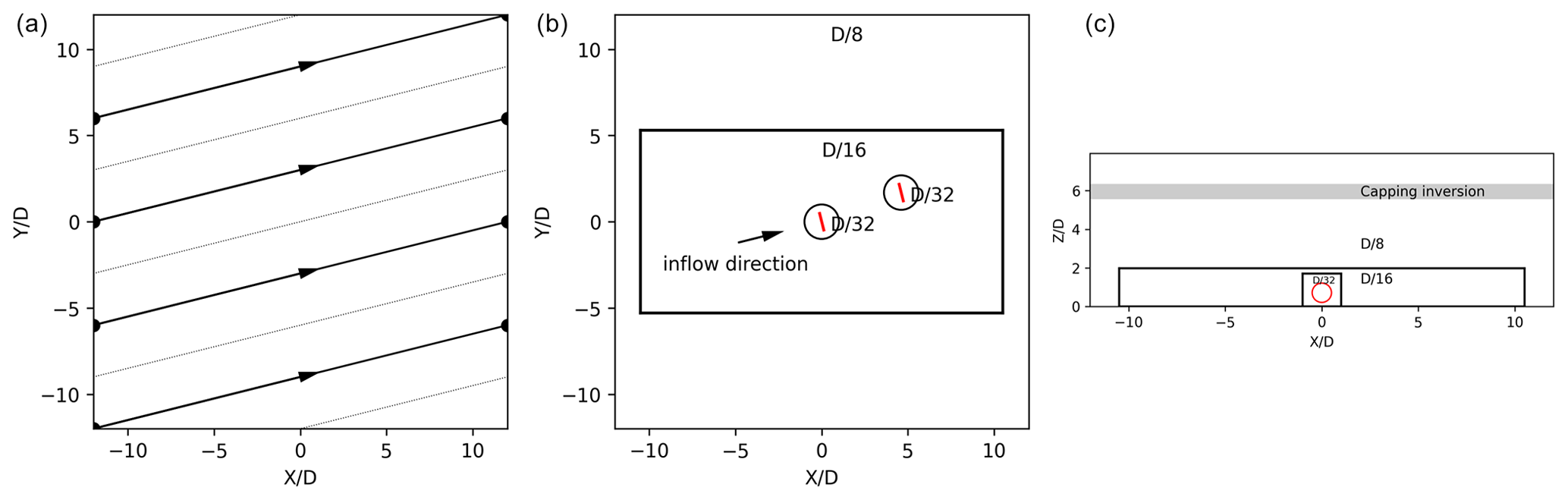
Figure 3Domain size and mesh refinement zones for the ABL inflow case: (a) total distance traveled by the coherent structure before entering again into the domain in the same position and mesh refinement zones in a (b) horizontal and (c) vertical plane.
2.3 Reference wind turbine
In the present study, the widely employed NREL 5 MW reference WT (Jonkman et al., 2009), which is equipped with a three-bladed rotor of diameter D=126 m and tower height H=90 m, is used for the computations. Regarding the WT operational configuration the turbine has two control regimes: one below the rated wind speed (Uref=11.4 m s−1), where ω grows linearly (with a λ=7.55) and θp=0∘, and one above the rated wind speed, where ω remains constant and θp increases. In contrast to the previous work (Navarro Diaz et al., 2019a), the CT and CP curves of the NREL 5 MW are in the present work not taken from Ponta et al. (2016) but use the two curves resulting from the ADM-airfoil and ALM-airfoil. This ensures a fair comparison between the actuator disk and actuator line model families.
The results are separated between the uniform and turbulent ABL inflow conditions. First, a single turbine is simulated with uniform inflow to compare all the variations in the ADM and the ALM proposed in this work. This comparison is done for a below-rated inflow velocity Uhub=8 m s−1. Once the models are tested in a single-turbine setting, another step in the inflow complexity is achieved, locating two turbines in a non-aligned layout, in order to test the models for a half-wake impact situation on the rotor plane. This pair of turbines is located under uniform and turbulent ABL inflow conditions, with Uhub=8 m s−1 at hub height. This difference in the turbulent condition will change the wake impact on the perturbed WT.
3.1 Uniform inflow
3.1.1 Single wind turbine
First, a preliminary mesh sensitivity study is necessary to find the dependency of the force's distribution and the wake on the number of cells along the diameter. This pre-study can be found in Sect. A in the Appendix. From the results obtained in this mesh sensitivity study, the resolution has been chosen for the simulations in this work. This choice aligns with recommendations from other authors for the ALM simulations under uniform and turbulent ABL inflow conditions (Asmuth et al., 2020, 2022).
Once the mesh resolution is chosen, the next step is the comparison of the six models for a basic case with a single turbine facing a uniform inflow velocity of Uhub=8 m s−1, a condition that determines Ω, CT and CP but not the local force calculation. In order to obtain the CT and CP for the analytical and numerical models, the ADM-airfoil and ALM-airfoil are run for all the velocities Uref in the productive range with constant λ=7.55, and the resulting values of CT and CP are saved in two tables, one for the ADM group and another one for the ALM group. The separation in two tables is required since the obtained coefficients are affected by the different tip and root corrections adopted in the ADM-airfoil and in the ALM-airfoil, respectively. These tables are used by the ADM-an, ADM-num, ALM-an and ALM-num. In Fig. 4 the normal fn and tangential fθ force distributions can be seen, separating the results in two groups, ADMs and ALMs. In both groups of models, the major differences can be found in the tip and root regions, while in the middle of the blade the constant circulation assumption matches very well with the calculations based on airfoil data. Specially for the tangential force distribution at the root, the models have large discrepancies due to the assumptions in the root correction compared to the use of airfoil data. It is important to notice that despite the use of tip correction in the ALM, there is a slight overestimation of fn and fθ in the last 10 % of the blade.
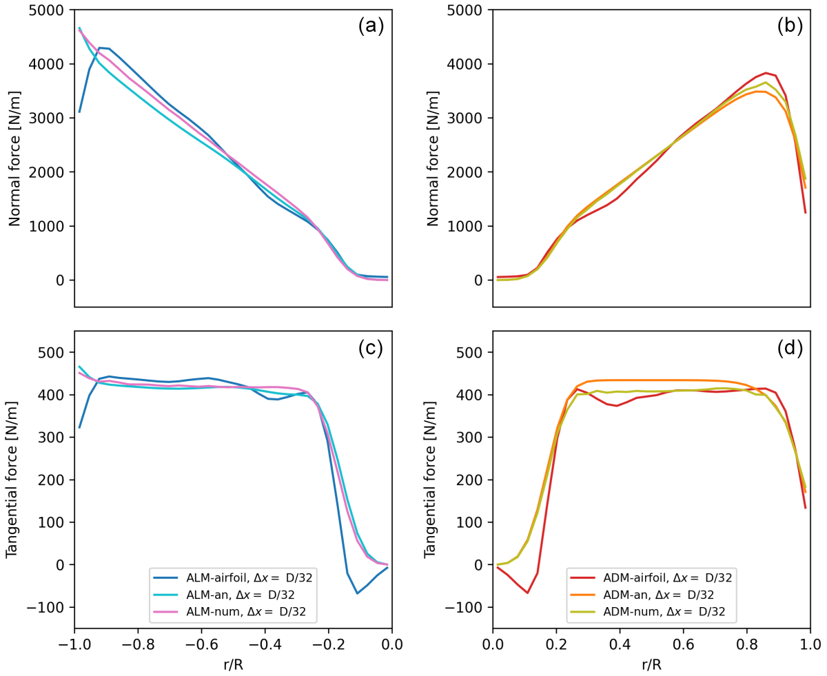
Figure 4Model comparison for the single-turbine case under uniform velocity inflow conditions of U∞=8 m s−1 and fixed conditions Uref=8 m s−1: normal fn (a, b) and tangential fθ (c, d) force distributions using different models.
In order to analyze how the differences in the force's distribution affect the wake, in Fig. 5 the velocity magnitude is compared at four distances downstream of the turbines: 1, 2.5, 5 and 7.5 D. The wakes obtained with each model are remarkably close, with the major differences located in the central part of the rotor. As expected, the wakes tend to collapse on the same shape at the far-wake region due to the use of the same CT. The non-turbulent inflow condition increases the necessary distance for the wake results to coincide, reaching in this case more than 7.5 D.
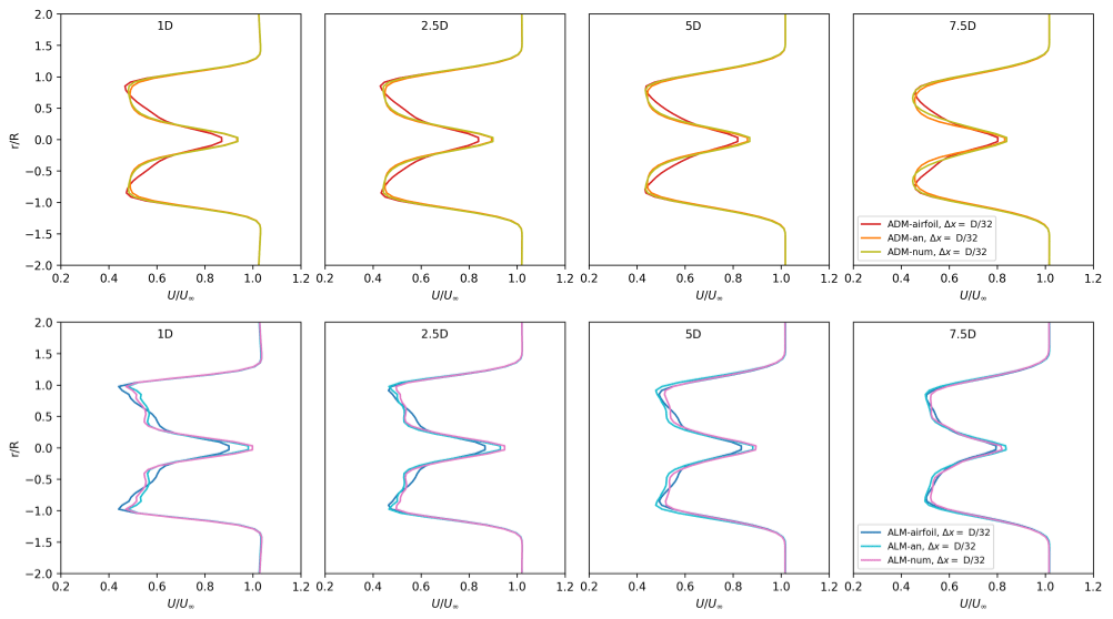
Figure 5Velocity magnitude comparison of the wake using different models for the single-turbine case under uniform velocity inflow conditions of U∞=8 m s−1: ADM (top panels) and ALM (bottom panels).
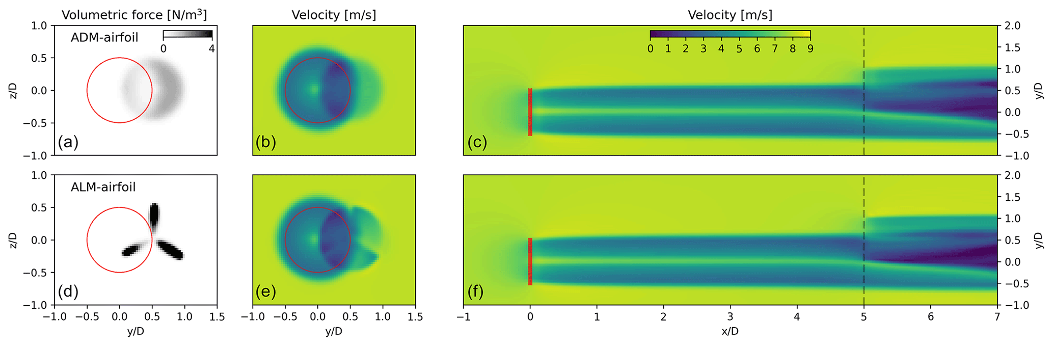
Figure 6Model comparison for two turbines under uniform velocity inflow conditions of U∞=8 m s−1, using the ADM-airfoil in WT1 and testing the ADM-airfoil and the ALM-airfoil in WT2: instantaneous force (a, d) and velocity (b, e) in a vertical plane at the WT2 location. The WT1 rotor plane is marked by the red circle. (c, f) Instantaneous velocity in a horizontal plane at hub height, where the WT2 vertical plane position is marked with a dashed line.
3.1.2 Wind turbine interaction
The next step is to analyze how the models perform under non-uniform inflow conditions, in this case when WT1 generates a wake which afterwards affects WT2. Particularly for this work, the ADM-airfoil is always used to simulate WT1 in order to create the same wake inflow condition for WT2. Also, in WT2 the reference velocity Uref is fixed, a condition that determines the rotation speed Ω. In order to find the Uref for WT2, a preliminary simulation is carried out using the ADM-airfoil also in WT2 but in which Uref is estimated based on the average velocity on the disk Ud. In order to find a relation between Ud and Uref, a pre-calculated table is used. Because the estimated value of Uref for each time step is different due to the non-uniform inflow, the value of Uref that will be used in the next simulations is computed by time-averaging the values, resulting in this case in Uref=5.992 m s−1, with a corresponding Ω=0.719 s−1.
Figure 6 shows the instantaneous volumetric force and velocity on a vertical plane at the WT2 position for the ADM-airfoil and ALM-airfoil. In the same figure the velocity field on a horizontal plane at hub height is shown. In the region of wake impact on the WT2 rotor the local reduction in the forces can be noticed in both the ADM-airfoil and ALM-airfoil due to a lower inflow velocity. Especially for the ALM-airfoil, every time that the blade passes this wake region, the forces are instantaneously reduced. For this transient problem, the period T is deduced as the time that the blade in WT2 (Ω=0.719 s−1) takes to move 120∘ (; s). In order to see how this transient problem affects the turbine power output, in Fig. 7 the power along four periods (11.6 s) using the three ALMs is shown. As expected, the ADM-airfoil cannot capture the variation in power and only reports a constant value (not shown in the figure), while all the ALMs show the same pattern when a blade enters and exits the wake. Taking ALM-airfoil as the reference, the normalized power amplitude is 0.28. ALM-airfoil is the model that reports the higher amplitude, followed by ALM-num and ALM-an.
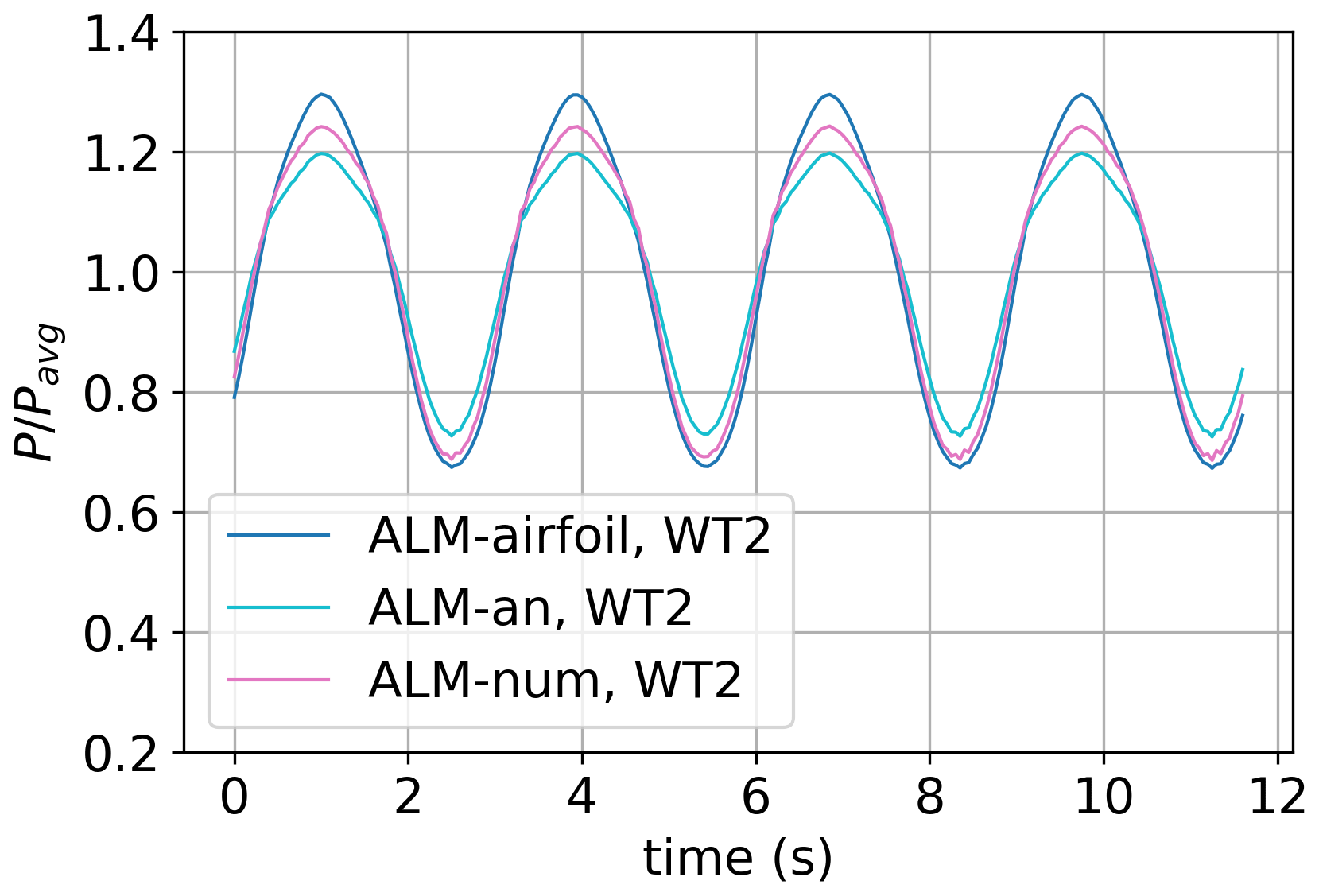
Figure 7ALM comparison of the time-varying power output P normalized with the time-averaged power Pavg for WT2 being partially waked by WT1. The rotational speed Ω is fixed in all the models.
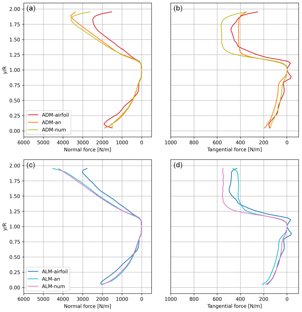
Figure 8Model comparison for two turbines under uniform velocity inflow conditions of U∞=8 m s−1: time-averaged (a, c) normal and (b, d) tangential force distributions for WT2 for the azimuthal angles ( from 0 to 1) and the azimuthal angles ( from 1 to 2).
In order to study how the models distribute the forces in this uneven spatial inflow, in Fig. 8 the average normal fn and tangential fθ force distributions on the WT2 rotor, for both the impacted and free side, are shown. When the ADMs are compared, the ADM-an and the ADM-num have a similar response at each side of the rotor, finding minor differences not only for the waked side but also for the free side. Compared to the more realistic ADM-airfoil, the tendencies in both sides are similar, with major differences on the free side. When the three ALMs are compared, similar observations can be obtained. It is important to notice that the overestimation of the normal force on the free side by the numeric approach is counteracted by an underestimation of the tangential force in the same rotor area. The major difference on the free side explains the reason why the peaks in the power output time series correspond to the moments when the models show the greatest differences. It can be noticed that the uniform laminar inflow induces a wake impact with a strong local velocity deficit on the rotor. This complex condition makes it difficult for simple analytical and numerical approaches to have satisfactory performance in the entire rotor area.
3.2 ABL inflow
The last step is to compare the model performance in a turbulent neutral ABL inflow condition, which is related to the problem of simulating wind farms in real field conditions. For this inflow condition, the same layout of two turbines as the uniform inflow case is simulated. At hub height a time-averaged velocity of U∞=8 m s−1 and a typical onshore site turbulence intensity, as measured with a cup anemometer, of approximately TIcup=9.75 % are specified.
As in the previous case, the ADM-airfoil is used to simulate WT1 in order to create the same wake inflow condition for WT2. Also, in WT2 the reference velocity Uref is fixed, a condition that determines the rotation speed Ω. Following the same procedure as for uniform free-stream inflow applied to the ABL case, the fixed values for WT2 are Uref=6.867 m s−1 with a corresponding Ω=0.823 s−1. It is important to remark that no change is needed in the analytical (ADM-an and ALM-an) or the numerical approaches (ADM-num and ALM-num) to be applied in turbulent inflows. This means that the analytical relations are still valid, as well as the calibration tables obtained for uniform flow.
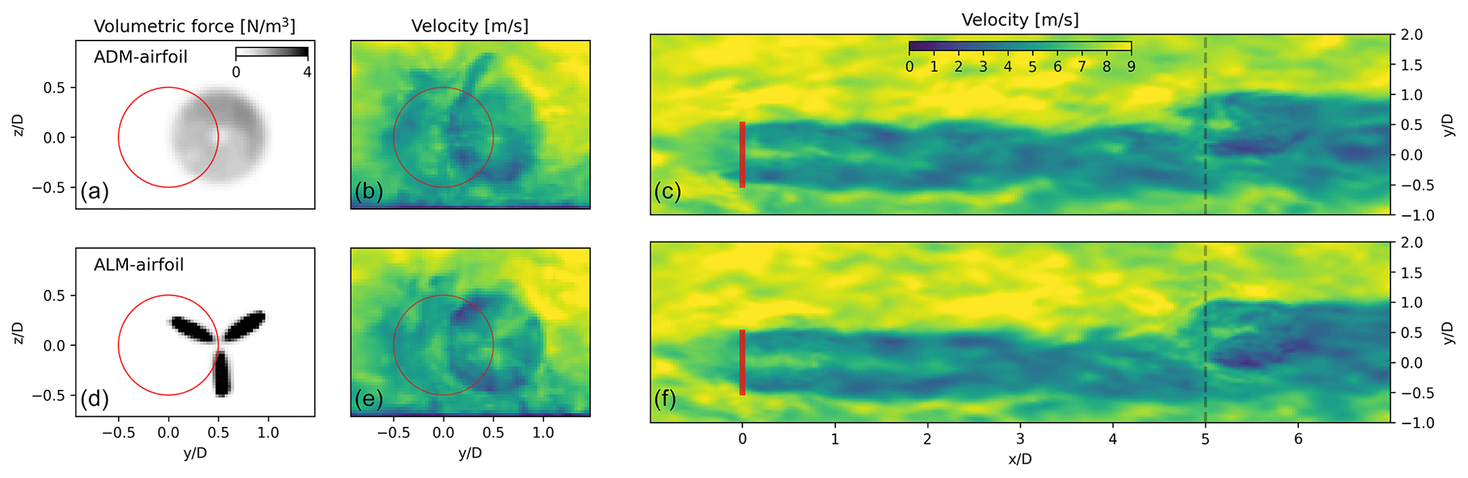
Figure 9Model comparison for two turbines in an ABL under horizontally averaged velocity inflow conditions at hub height of U∞=8 m s−1: instantaneous force (a, d) and velocity (b, e) in a vertical plane at the WT2 location. The WT1 rotor position is indicated with a red circle. (c, f) Instantaneous velocity in a horizontal plane position at hub height, with the WT2 vertical plane marked with a dashed line.
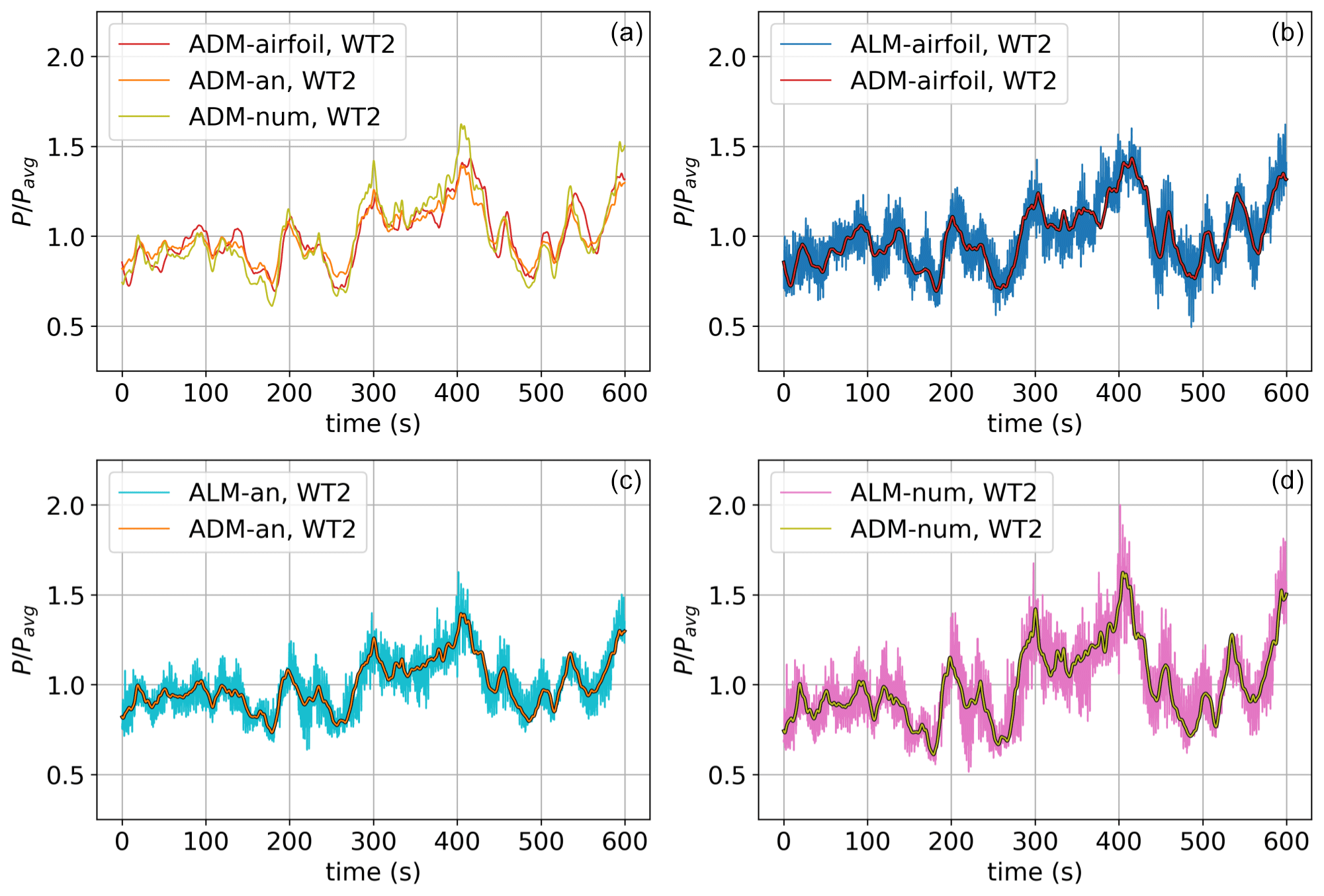
Figure 10Model comparison of the power output time variation normalized with its time-averaged value (Pavg) for two turbines in the ABL under average velocity inflow conditions at hub height of U∞=8 m s−1. (a) Comparison of the three ADMs. (b–d) The comparisons of the same groups of ADMs and ALMs are shown.
In Fig. 9 the solutions for the ADM-airfoil and the ALM-airfoil are presented, showing the instantaneous volumetric force and velocity on a vertical plane normal to the flow at the WT2 position, as well as the velocity on a horizontal plane at hub height. It can be noticed that the local force distribution on the ADM reacts to the non-uniform spatial distribution of the velocity field on the rotor plane. As can be seen in the instantaneous velocity field, in this complex inflow condition the models need to respond not only to the partial-wake impact but also to the time-varying velocity due to the vertical boundary layer profile. This response is clearly different between the ADM-airfoil and the ALM-airfoil. To visualize this difference, in Fig. 10 the time variation in the power output of both models during a 10 min period is shown. The power output of the ADM-airfoil is only related to the variation in the average velocity over the disk. On the other hand, the ALM-airfoil in addition manages to correctly capture the power variation due to the blades passing through areas of low velocity, including the partial-wake and the non-uniform vertical wind profiles. When the three ADMs are compared, a good match of the simplified models with the ADM-airfoil is achieved. The major differences are seen when the power reaches local maximums or minimums, registering a stronger response in the ALM-num. When the ADM and the ALM based on the same formulation are compared, it can always be seen that the ALM can capture additional power variations.
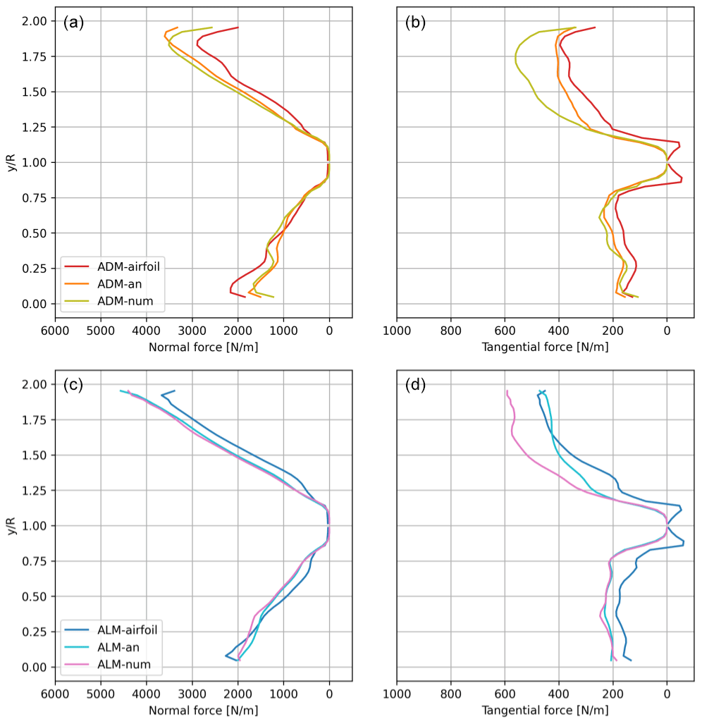
Figure 11Model comparison for two turbines in an ABL under average velocity inflow conditions of Uhub=8 m s−1: average (a, c) normal and (b, d) tangential force distributions for WT2 for the azimuthal angles 90±10 ( from 0 to 1) and the azimuthal angles 270±10 ( from 1 to 2).
In order to analyze how all the models distribute the forces in this turbulent wake inflow, in Fig. 11 the time-averaged normal fn and tangential fθ force distributions on the WT2 rotor are shown for both the wake-impacted and free sides. Due to the ambient turbulence produced by the ABL flow the wake decay and expansion are larger, resulting in a more distributed wake impact over the rotor area and less of a velocity deficit in the impacted half-side of the rotor. Compared to the uniform free-stream inflow case, a similar trend in the force distributions can be found at both sides of the rotor. Given that in this ABL case the time-averaged velocity varies in both the lateral and vertical directions, the force distributions on the rotor area are shown in Figs. 12 and 13. In Fig. 12 the normal force distribution over the impacted WT2 rotor for the six models is compared. It is clear how analytical and numerical approaches manage to follow the same trend compared with the airfoil formulation, finding the highest force values in the upper part of the free side of the rotor and the lowest values in the bottom part of the waked side. Both the analytical and numerical approaches slightly overestimate values on the free side of the rotor, particularly the ADM-num and the ALM-num. In Fig. 13 a similar comparison is shown for the tangential force distribution, finding again the same overestimation of forces on the free side of the rotor by the ADM-num and the ALM-num. It is easy to notice that the force distribution along the radius is less homogeneous than in the uniform inflow case. This problem is due to the local velocity interpolation being affected by the non-aligned position of the rotor area with the mesh, which affects in the same manner all the models. Later studies would have to analyze this phenomenon and how to reduce its effect on the results.
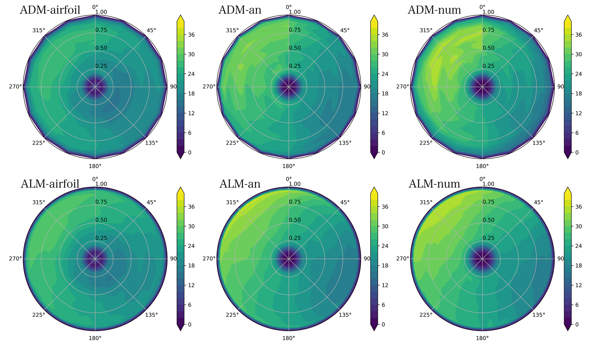
Figure 12Model comparison for the time-averaged normal force distribution (N m−2) on the impacted rotor (WT2) for ABL inflow. The wake from WT1 impacts the right side of the rotor plane (Fig. 1).
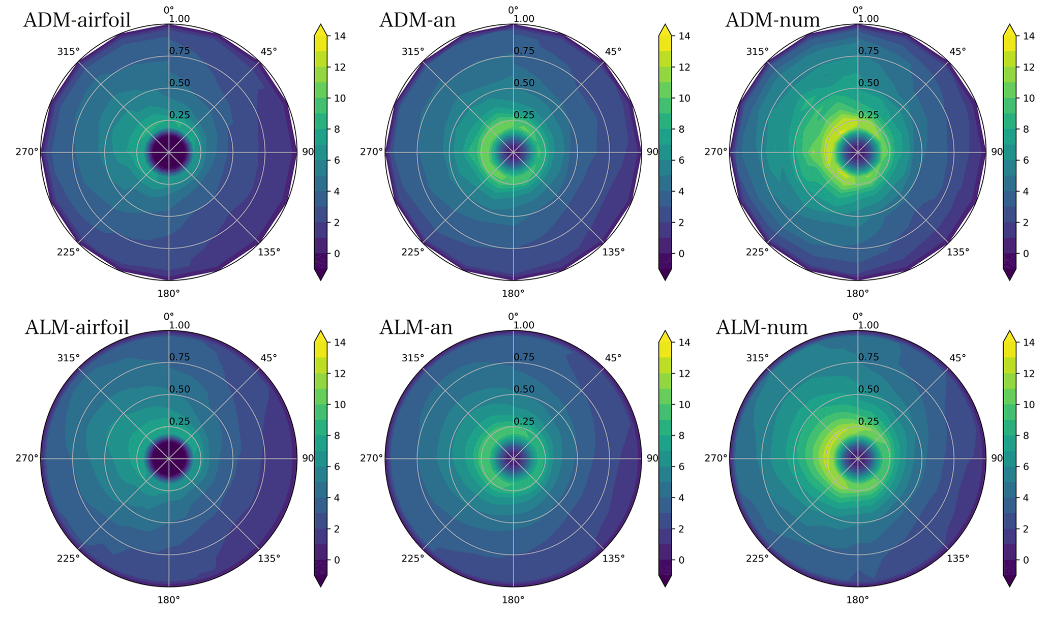
Figure 13Model comparison for the time-averaged tangential force distribution (N m−2) on the impacted rotor (WT2) for ABL inflow. The wake from WT1 impacts the right side of the rotor plane.
In this work the previous developments for an ADM with local force calculations based on analytical (Sørensen et al., 2020) or numerical (Navarro Diaz et al., 2019b) approaches are extended to the ALM. These two approaches share the advantage that only limited and basic manufacturer WT information is needed, i.e., any combination of the thrust and power coefficient and the tip speed ratio. The ADM and the ALM built from these two approaches are compared with the equivalent advanced models based on blade element theory, which provides more realistic force distributions but requires information about the operating setting and the geometric and aerodynamic characteristics of the blade.
When a single turbine facing a uniform free-stream inflow is simulated, a close normal and tangential force distribution along the blade is found between all the models. The difficulties in capturing the root and tip force distributions obtained with the airfoil data are the major source of differences with the simpler models. The two new ALMs have the same distribution as the corresponding ADMs, with the only difference being the particular tip correction needed in the ALMs.
The models are tested in the challenging case of a WT partially affected by an up-steam wake, for both uniform non-turbulent inflow and turbulent neutral ABL. The analytical and numerical approaches manage to correctly capture the different force distributions at the different regions of the rotor, with a consistent overestimation of the normal force on the free side and a sub-estimation on the waked side. Looking at the tangential force distribution, the numerical approach tends to overestimate the values on the free side. In general, the analytical approach shows a slightly better performance in wake impact cases compared to the numerical one. The three ALMs show the additional capacity of capturing higher frequencies in the power output variation in time. In the uniform inflow case, the clear sign on how the power is reduced when one of the blades passes through the wake region is captured in an equivalent way by the three models. This added feature of the ALM is also visible in the ABL inflow case. The numerical approach has shown higher power fluctuations in both the ADM and the ALM. Finally, the extension of both the analytical and numerical approaches from the ADM to the ALM has shown promising results, opening the possibility to simulate commercial wind farms in transient inflows with the ALM without the restriction of private manufacturer blade data.
For this study the well-known ADM-airfoil and the ALM-airfoil are chosen. The inflow velocity is fixed at Uhub=8 m s−1 and the tip speed ratio at λ=7.55 in order to compare the results with the ones published by Asmuth et al. (2020). At this velocity, the rotational speed is approximately Ω=9.15 rpm = 0.95 s−1. These authors carried out a mesh sensitivity study for the ALM-airfoil without tip correction. Particularly, the results for using the software EllipSys3D are chosen for comparison.
This pair of models is tested for a wide range of mesh resolutions, which are defined by the cell size in relation to the rotor diameter D: , , , and . It is important to remark that the separation between nodes Δb and ε are defined in relation to the cell size Δx. In the case of the ADM, the number of lines nl (Eq. 1) also depends on the mesh resolution.
In Fig. A1 it can be seen how the maximum instantaneous vorticity in the near wake changes when the mesh resolution is increased. In the case of the ADM-airfoil, the values of vorticity in the tip and root regions increase when the cell size is reduced. On the other hand, in the ALM-airfoil this pattern is also followed by the development of tip and root helical tubes when the resolution is closer to or higher. The comparison of the vorticity fields between the ADM and the ALM and the dependency of the development of helical structures with the mesh resolution were also studied by Martinez et al. (2012), who arrived at similar conclusions as this sensitivity study.
In Fig. A2 the normal fn and tangential fθ force distributions along the blade for both models are shown. In the case of the ADM-airfoil, when the resolution is increased, the forces near the tip and root regions are reduced, maintaining the values in the rest of the disk. For the ALM-airfoil this pattern is also seen but with minor changes in the values. A good agreement between the results of Asmuth et al. (2020) and the ones obtained in this work can be seen along the blade. Expected small differences are found due to the tip correction adopted in this work, where ε varies depending on the radial position.
In order to see how the force distributions converge when the mesh is refined, the L2 error for the normal force fn distribution is calculated for 32 fixed radial positions j along the blade as
where is the solution for the higher resolution (). The same expression is used for the tangential force fθ. In Fig. A3 it can be observed how the L2 error is reduced rapidly when the mesh is refined, showing similar values for both models. The error for the normal force is lower compared to the results for the tangential force. For the specific resolution, the L2 errors in the normal force are 1.2 % and 1.4 % for the ADM-airfoil and ALM-airfoil, respectively. In the case of the tangential force, the errors are 3.5 % and 3.8 %. The changes in the forces are reflected in the thrust T and power output P, as can be seen also in Fig. A3. In the case of the ADM-airfoil, T and P are reduced with the increasing resolution. This relation between the reduction in ε, or reduction in the cell size Δx, and the decrease in the power was also found by Martinez et al. (2012). When the resolution is compared with the higher resolution, the thrust force is 0.5 % higher with the ADM-airfoil and 0.7 % with the ALM-airfoil. The power output is 2.0 % higher with the ADM-airfoil and 1.7 % with the ALM-airfoil.
From the results obtained in this mesh sensitivity study, the resolution has been chosen for the simulations in this work. This choice is a compromise between a low L2 error in the force distributions and the turbine outputs and the affordable computational cost for ABL simulations. This cost is especially important in this work due to the fact that the new ALMs, based on basic manufacture information, are created in order to open the possibility to simulate big wind farms with commercial WTs and long transient ABL problems.

Figure A1Mesh sensitivity study for the ADM-airfoil and the ALM-airfoil: instantaneous vorticity on a plane at hub height. Part of the extension of the force distributions is marked with a rectangle, assigning a total rectangle width of 2ε.

Figure A2Mesh sensitivity study for the ADM-airfoil and the ALM-airfoil: normal fn (a, b) and tangential fθ (c, d) force distributions along the blade using different mesh resolutions. The EllipSys LES result from Asmuth et al. (2020) for the resolution of the ALM-airfoil (no tip correction) is also plotted.
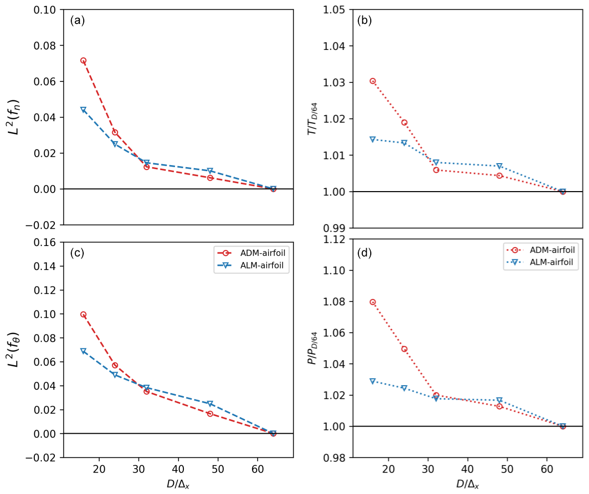
Figure A3Mesh sensitivity study for the ADM-airfoil and the ALM-airfoil: (a, c) L2 error for the normal fn (a) and tangential fθ (c) force distributions in different mesh resolutions. The error is calculated by comparing with the distribution of the higher-resolution case. Thrust T (b) and power P (d), where the values are divided by the value obtained with the higher resolution.
The SOWFA framework on which this work is based is made available by NREL (https://github.com/NREL/SOWFA/; NREL, 2023). The code developed for the new models proposed in this work is not publicly available.
All data presented in this study can be made available upon request.
GPND developed the model code, performed the simulations, plotted the results and wrote the manuscript. ADO, HA, JNS and SI contributed with ideas, corrections and modifications both in the choice of models and in the results and text.
At least one of the (co-)authors is a member of the editorial board of Wind Energy Science. The peer-review process was guided by an independent editor, and the authors also have no other competing interests to declare.
Publisher's note: Copernicus Publications remains neutral with regard to jurisdictional claims in published maps and institutional affiliations.
The simulations were performed on resources provided by the Swedish National Infrastructure for Computing (SNIC).
This paper was edited by Alessandro Bianchini and reviewed by two anonymous referees.
Abkar, M., Sharifi, A., and Porté-Agel, F.: Wake flow in a wind farm during a diurnal cycle, J. Turbulence, 17, 420–441, 2016. a, b
Arthur, R. S., Mirocha, J. D., Marjanovic, N., Hirth, B. D., Schroeder, J. L., Wharton, S., and Chow, F. K.: Multi-scale simulation of wind farm performance during a frontal passage, Atmosphere, 11, 245, https://doi.org/10.3390/atmos11030245, 2020. a
Asmuth, H., Olivares-Espinosa, H., and Ivanell, S.: Actuator line simulations of wind turbine wakes using the lattice Boltzmann method, Wind Energ. Sci., 5, 623–645, https://doi.org/10.5194/wes-5-623-2020, 2020. a, b, c, d, e, f
Asmuth, H., Navarro Diaz, G. P., Madsen, H. A., Branlard, E., Forsting, A. R. M., Nilsson, K., Jonkman, J., and Ivanell, S.: Wind turbine response in waked inflow: A modelling benchmark against full-scale measurements, Renew. Energy, 191, 868–887, 2022. a, b
Bossuyt, J., Howland, M. F., Meneveau, C., and Meyers, J.: Wind tunnel study of the power output spectrum in a micro wind farm, J. Phys.: Conf. Ser., 753, 072002, https://doi.org/10.1088/1742-6596/753/7/072002, 2016. a
Churchfield, M., Lee, S., Moriarty, P., Martinez, L., Leonardi, S., Vijayakumar, G., and Brasseur, J.: A large-eddy simulation of wind-plant aerodynamics, in: 50th AIAA Aerospace Sciences Meeting including the New Horizons Forum and Aerospace Exposition, 9–12 January 2012, Nashville, Tennessee, USA, p. 537, https://doi.org/10.2514/6.2012-537, 2012a. a
Churchfield, M. J., Lee, S., Michalakes, J., and Moriarty, P. J.: A numerical study of the effects of atmospheric and wake turbulence on wind turbine dynamics, J. Turbulence, 13, N14, https://doi.org/10.1080/14685248.2012.668191, 2012b. a, b, c
Dağ, K. O. and Sørensen, J. N.: A new tip correction for actuator line computations, Wind Energy, 23, 148–160, 2020. a, b
Englberger, A. and Dörnbrack, A.: Impact of the diurnal cycle of the atmospheric boundary layer on wind-turbine wakes: a numerical modelling study, Bound.-Lay. Meteorol., 166, 423–448, 2018. a
Glauert, H.: Airplane propellers, in: Aerodynamic theory, Springer, 169–360, https://doi.org/10.1007/978-3-642-91487-4_3, 1935. a, b
Howland, M. F., Bossuyt, J., Martínez-Tossas, L. A., Meyers, J., and Meneveau, C.: Wake structure in actuator disk models of wind turbines in yaw under uniform inflow conditions, Journal of Renewable and Sustainable Energy, 8, 043301, https://doi.org/10.1063/1.4955091, 2016. a
Jha, P. K. and Schmitz, S.: Actuator curve embedding–an advanced actuator line model, J. Fluid Mech., 834, R2, https://doi.org/10.1017/jfm.2017.793, 2018. a, b
Jonkman, J., Butterfield, S., Musial, W., and Scott, G.: Definition of a 5-MW reference wind turbine for offshore system development, Technical Report No. NREL/TP-500-38060, National Renewable Energy Laboratory, Golden, CO, https://doi.org/10.2172/947422, 2009. a
Marjanovic, N., Mirocha, J. D., Kosović, B., Lundquist, J. K., and Chow, F. K.: Implementation of a generalized actuator line model for wind turbine parameterization in the Weather Research and Forecasting model, J. Renew. Sustain. Energ., 9, 063308, https://doi.org/10.1063/1.4989443, 2017. a
Martinez, L., Leonardi, S., Churchfield, M., and Moriarty, P.: A comparison of actuator disk and actuator line wind turbine models and best practices for their use, in: 50th AIAA Aerospace Sciences Meeting including the New Horizons Forum and Aerospace Exposition, 9–12 January 2012, Nashville, Tennessee, USA, p. 900, https://doi.org/10.2514/6.2012-900, 2012. a, b, c, d
Munters, W., Meneveau, C., and Meyers, J.: Shifted periodic boundary conditions for simulations of wall-bounded turbulent flows, Phys. Fluids, 28, 025112, https://doi.org/10.1063/1.4941912, 2016. a
Nathan, J., Masson, C., Dufresne, L., and Churchfield, M. J.: Analysis of the sweeped actuator line method, in: E3S Web of Conferences, vol. 5, National NREL – Renewable Energy Lab., Golden, CO, USA, https://doi.org/10.1051/e3sconf/20150501001, 2015. a
Nathan, J., Forsting, A. R. M., Troldborg, N., and Masson, C.: Comparison of OpenFOAM and EllipSys3D actuator line methods with (NEW) MEXICO results, J. Phys.: Conf. Ser., 854, 012033, https://doi.org/10.1088/1742-6596/854/1/012033, 2017. a
Nathan, J., Masson, C., and Dufresne, L.: Near-wake analysis of actuator line method immersed in turbulent flow using large-eddy simulations, Wind Energ. Sci., 3, 905–917, https://doi.org/10.5194/wes-3-905-2018, 2018. a
Navarro Diaz, G. P., Saulo, A. C., and Otero, A. D.: Comparative study on the wake description using actuator disc model with increasing level of complexity, J. Phys.: Conf. Ser., 1256, 012017, https://doi.org/10.1088/1742-6596/1256/1/012017, 2019a. a, b, c, d, e, f, g, h, i
Navarro Diaz, G. P., Saulo, A. C., and Otero, A. D.: Wind farm interference and terrain interaction simulation by means of an adaptive actuator disc, J. Wind Eng. Indust. Aerodynam., 186, 58–67, 2019b. a, b, c, d
Navarro Diaz, G. P., Saulo, A. C., and Otero, A. D.: Full wind rose wind farm simulation including wake and terrain effects for energy yield assessment, Energy, 237, 121642, https://doi.org/10.1016/j.energy.2021.121642, 2021. a
NREL: SOWFA, GitHub [code], https://github.com/NREL/SOWFA/, last access: 21 March 2023. a
Ponta, F. L., Otero, A. D., Lago, L. I., and Rajan, A.: Effects of rotor deformation in wind-turbine performance: the dynamic rotor deformation blade element momentum model (DRD–BEM), Renew. Energy, 92, 157–170, 2016. a
Porté-Agel, F., Wu, Y.-T., Lu, H., and Conzemius, R. J.: Large-eddy simulation of atmospheric boundary layer flow through wind turbines and wind farms, J. Wind Eng. Indust. Aerodynam., 99, 154–168, 2011. a, b
Porté-Agel, F., Bastankhah, M., and Shamsoddin, S.: Wind-turbine and wind-farm flows: a review, Bound.-Lay. Meteorol., 174, 1–59, 2020. a
Sanderse, B., Pijl, S., and Koren, B.: Review of computational fluid dynamics for wind turbine wake aerodynamics, Wind Energy, 14, 799–819, 2011. a
Sørensen, J. N. and Andersen, S. J.: Validation of analytical body force model for actuator disc computations, J. Phys.: Conf. Ser., 1618, 052051, https://doi.org/10.1088/1742-6596/1618/5/052051, 2020. a, b
Sørensen, J. N. and Kock, C. W.: A model for unsteady rotor aerodynamics, J. Wind Eng. Indust. Aerodynam., 58, 259–275, 1995. a
Sørensen, J. N. and Myken, A.: Unsteady actuator disc model for horizontal axis wind turbines, J. Wind Eng. Indust. Aerodynam., 39, 139–149, 1992. a
Sørensen, J. N. and Shen, W. Z.: Numerical modeling of wind turbine wakes, J. Fluids Eng., 124, 393–399, 2002. a, b
Sørensen, J. N., Mikkelsen, R. F., Henningson, D. S., Ivanell, S., Sarmast, S., and Andersen, S. J.: Simulation of wind turbine wakes using the actuator line technique, Philos. T. Roy. Soc. A, 373, 20140071, https://doi.org/10.1098/rsta.2014.0071, 2015. a
Sørensen, J. N., Nilsson, K., Ivanell, S., Asmuth, H., and Mikkelsen, R. F.: Analytical body forces in numerical actuator disc model of wind turbines, Renew. Energy, 147, 2259–2271, 2020. a, b, c, d, e, f, g, h, i
Stevens, R. J., Martínez-Tossas, L. A., and Meneveau, C.: Comparison of wind farm large eddy simulations using actuator disk and actuator line models with wind tunnel experiments, Renew. Energy, 116, 470–478, 2018. a
Stieren, A., Gadde, S. N., and Stevens, R. J.: Modeling dynamic wind direction changes in large eddy simulations of wind farms, Renew. Energy, 170, 1342–1352, 2021. a
van der Laan, M. P., Sørensen, N. N., Réthoré, P.-E., Mann, J., Kelly, M. C., Troldborg, N., Schepers, J. G., and Machefaux, E.: An improved k–ε model applied to a wind turbine wake in atmospheric turbulence, Wind Energy, 18, 889–907, 2015. a, b, c, d, e
van der Laan, M. P., Andersen, S. J., Réthoré, P. E., Baungaard, M., Sørensen, J. N., and Troldborg, N.: Faster wind farm AEP calculations with CFD using a generalized wind turbine model, J. Phys.: Conf. Ser., 2265, 022030, https://doi.org/10.1088/1742-6596/2265/2/022030, 2022. a
Wang, J., Wang, C., Castañeda, O., Campagnolo, F., and Bottasso, C.: Large-eddy simulation of scaled floating wind turbines in a boundary layer wind tunnel, J. Phys.: Conf. Ser., 1037, 072032, https://doi.org/10.1088/1742-6596/1037/7/072032, 2018. a
Yoshizawa, A.: Statistical theory for compressible turbulent shear flows, with the application to subgrid modeling, Phys. Fluids, 29, 2152–2164, 1986. a
Zhong, W., Wang, T. G., Zhu, W. J., and Shen, W. Z.: Evaluation of Tip Loss Corrections to AD/NS Simulations of Wind Turbine Aerodynamic Performance, Appl. Sci., 9, 4919, https://doi.org/10.1063/1.865552, 2019. a