the Creative Commons Attribution 4.0 License.
the Creative Commons Attribution 4.0 License.
 | 15 May 2024
Aerodynamic characterisation of a thrust-scaled IEA 15 MW wind turbine model: experimental insights using PIV data
André Ribeiro
Koen Boorsma
Carlos Ferreira
This study presents results from a wind tunnel experiment on a three-bladed horizontal axis wind turbine. The model turbine is a scaled-down version of the IEA 15 MW reference wind turbine, preserving the non-dimensional thrust distribution along the blade.
Flow fields were captured around the blade at multiple radial locations using particle image velocimetry. In addition to these flow fields, this comprehensive dataset contains spanwise distributions of bound circulation, inflow conditions and blade forces derived from the velocity field. As such, the three blades' aerodynamics are fully characterised. It is demonstrated that the lift coefficient measured along the span agrees well with the lift polar of the airfoil used in the blade design, thereby validating the experimental approach.
This research provides a valuable public experimental dataset for validating low- to high-fidelity numerical models simulating state-of-the-art wind turbines. Furthermore, this article establishes the aerodynamic properties of the newly developed model wind turbine, creating a baseline for future wind tunnel experiments using this model.
- Article
(5061 KB) - Full-text XML
- BibTeX
- EndNote


Wind tunnel experiments are vital in progressing horizontal axis wind turbine (HAWT) technology. They help in improving the understanding of e.g. the turbine's aerodynamic, aeroelastic or acoustic characteristics. Equally important, the gathered data can be used to validate and improve numerical models that aim to simulate reality as closely as possible.
In light of these two goals, arguably the two most relevant experiments on HAWTs are the Unsteady Aerodynamics Experiment (UAE) and the Model Rotor Experiment in Controlled Conditions (MEXICO). NREL executed the UAE in multiple phases. While Phases I–IV, conducted between 1989 and 1997, were field experiments (Butterfield et al., 1992; Simms et al., 1999), Phase VI was a wind tunnel experiment conducted in 2000. A two-bladed rotor of 10 m diameter was heavily instrumented and placed in the NASA Ames wind tunnel (Hand et al., 2001). The MEXICO experiment was conducted in 2006 in the German–Dutch Wind Tunnel (DNW). Detailed aerodynamic measurements, including pressure, loads and 3D flow field characteristics using particle image velocimetry (PIV), were taken on a three-bladed rotor with 4.5 m diameter (Schepers and Snel, 2007; Boorsma and Schepers, 2009). Its successor project “New Mexico” was conducted in 2014 to obtain additional data (Boorsma and Schepers, 2015). The results of these two experimental campaigns have been analysed in great detail and have been used for the validation and calibration of simulation tools of varying fidelity. For an extensive review of the literature related to these two experiments, the reader is referred to the work of Schepers and Schreck (2018).
Given the success of these two experiments, the existing databases were extended by conducting further experiments on scaled versions of the two rotors. The wake of a 1:8 scaled version of the UAE Phase VI rotor was measured using PIV by Xiao et al. (2011). At the Korean Aerospace Research Institute (KARI), Cho and Kim (2014) tested the Reynolds number effect on torque and power on a 1:5 scaled model of the UAE Phase VI turbine. Comparable experiments were done by the same researchers for a 2:4.5 scaled version of the MEXICO rotor (Cho and Kim, 2012). The Spanish National Institute for Aerospace Technology (INTA) tested a 1:4 scaled MEXICO rotor. Results of the scaled models are compared against the original MEXICO data in IEA Task 29 by Schepers et al. (2012).
Complementary to experimental investigations, HAWTs are studied extensively using numerical simulations. To enable numerical benchmarks between different simulation tools and to facilitate collaboration between academic and industrial research, multiple reference wind turbine (RWT) models have been developed in recent years, e.g. the NREL 5 MW RWT (Jonkman et al., 2009), the DTU 10 MW RWT (Bak et al., 2013) and the IEA 15 MW RWT (Gaertner et al., 2020). While not representing existing wind turbines, these open-source reference models reflect current trends and developments of HAWT technology. Wind tunnel campaigns with scaled versions of these reference wind turbines have been conducted to provide experimental datasets that can be used to validate numerical simulations. Berger et al. (2018) developed a model turbine based on the NREL 5 MW RWT, which has since been used to study dynamic inflow phenomena due to pitch steps (Berger et al., 2021) and fluid–structure interaction by means of photogrammetry (Langidis et al., 2022; Nietiedt et al., 2022). Fontanella et al. (2021a) ran experiments on a scaled DTU 10 MW wind turbine mimicking the motions of a floating offshore wind turbine (FOWT). In addition to load cell measurements on the turbine, the wake was characterised using PIV measurements. Similar experiments were conducted by Taruffi et al. (2024), extending the mimicked floater motions to six degrees of freedom and larger amplitudes and frequencies. Fontanella et al. (2022) performed another set of experiments on a 1:100 scaled model of the IEA 15 MW RWT developed by Allen et al. (2020). Here, rotor loads were measured using load cells, and the wake was characterised using hot-wire velocity measurements. A 1:70 scaled model of the IEA 15 MW was tested by Kimball et al. (2022) with a focus on verifying thrust and torque curves and validating the utilised pitch controller. While these studies on scaled-down versions of the RWTs provide valuable data regarding rotor-level aerodynamics, they lack more detailed data on the blade level.
Such blade-level data can be obtained using non-intrusive measurement techniques such as laser Doppler velocimetry (LDV) or stereoscopic particle image velocimetry (SPIV). Phengpom et al. (2015a, b, 2016) studied the flow field in the direct vicinity of the blade using LDV. Akay et al. (2013) researched the vortex structure around the blade root of a two-bladed wind turbine with a 2 m diameter based on SPIV measurements. Similarly, Lignarolo et al. (2014) investigated the wake development of a smaller model (two blades, 0.6 m diameter) focusing on the tip vortices. Continuing this line of research, the generation of the tip vortex was investigated in more detail on a different two-bladed wind turbine model of 2 m diameter by Micallef et al. (2014, 2015). Furthermore, and most relevant to the present work, SPIV was employed to derive the spanwise blade load distribution of a HAWT in axial and yawed inflow by del Campo et al. (2014, 2015).
The present work studies the spanwise aerodynamic characteristics of a 1:133 scaled model of the IEA 15 MW RWT and thus of the most recent available reference wind turbine. SPIV is used to measure the flow field around various radial sections of the blade and consequently to derive the spanwise aerodynamic properties of this model wind turbine. By characterising the blades in terms of induction values, inflow angle and angle of attack, circulation, and blade loads, this study provides a more complete dataset of blade-level aerodynamics than previous wind tunnel experiments. As such, this research aims to enable further multi-fidelity numerical benchmarking as well as to establish a reference dataset that can be used as a starting point for future experimental studies on this wind tunnel model turbine.
This paper is structured as follows: Sect. 2 describes the scaling approach used to develop the wind tunnel model's blades. Furthermore, details of the experimental setup are given and the equations used to derive blade aerodynamic quantities from the measured flow fields are provided. Section 3 initially details the challenge of estimating deviations from the design twist distribution. It then presents the results of the experimental campaign in terms of flow fields, distributed blade aerodynamics and airfoil polars. Finally, conclusions are drawn in Sect. 4 and an outlook for further research is given.
2.1 Scaled wind turbine model
The model HAWT tested in this experiment is a scaled version of the IEA 15 MW RWT (Gaertner et al., 2020), preserving non-dimensional thrust. The main model characteristics are given in Table 1 alongside their full-scale equivalents.
Table 1Specifications of the IEA 15 MW RWT and the scaled wind tunnel model.
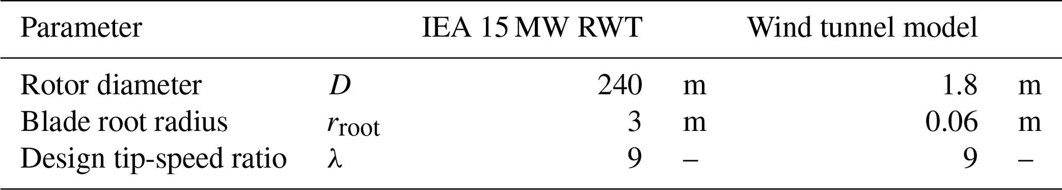
The geometric scaling factor of 1:133 applied to the rotor diameter cannot be maintained at the blade root. Here, mechanical and electronic components necessitate a larger blade root radius, leading to a scaling factor of 1:50. The ratio of root to tip radius is in close agreement with comparable wind tunnel models; see Fontanella et al. (2022).
Multiple challenges occur when creating a scaled-down wind tunnel model of a wind turbine. Arguably, the largest challenge lies in the fact that the chord Reynolds number Rec present on a full-scale wind turbine generally cannot be achieved in a wind tunnel. A difference in Rec of multiple orders of magnitude necessitates the use of airfoils designed explicitly for low Reynolds numbers. One such airfoil is the SD7032 airfoil, which has a maximum relative thickness of 10 % and was characterised experimentally by Fontanella et al. (2021b). The lift and drag coefficient of the SD7032 airfoil for different Reynolds numbers is given in Fig. 1. A characteristic of this airfoil, making it useful for small-scale wind turbines, is the relative insensitivity of the lift polar to the Reynolds number over a large range of angles of attack. The well-documented wind tunnel polars, as well as the airfoil's application in comparable wind tunnel campaigns (Kimball et al., 2022; Fontanella et al., 2022), motivated the choice for the SD7032 airfoil.
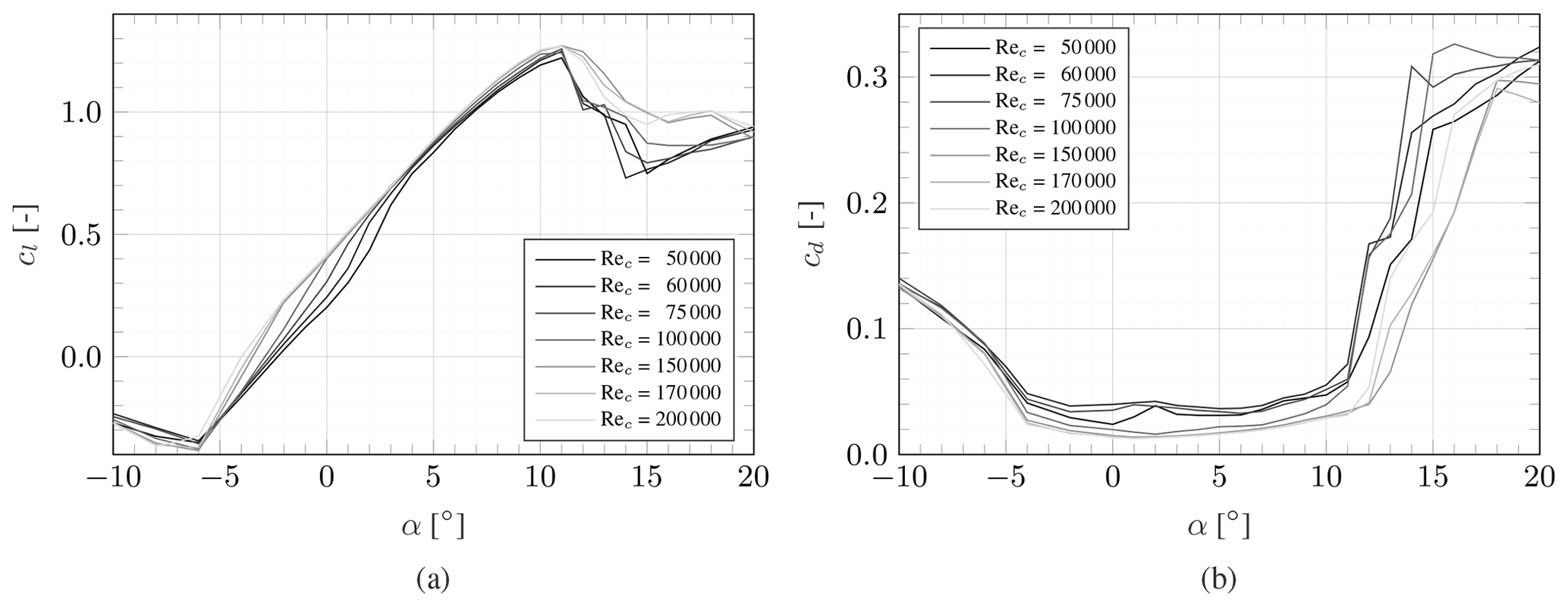
Figure 1Lift coefficient cl (a) and drag coefficient cd (b) of the SD7032 airfoil for varying Reynolds numbers (Fontanella et al., 2021b).
Instead of using various airfoils along the span, the developed model blades are defined by this single airfoil, which transitions into a cylindrical section at the blade root. The polars of the wind tunnel model differ from those of the airfoils used on the full-scale turbine. Thus, even at identical angles of attack, the non-dimensionalised lift distribution will differ between the model and original. Bayati et al. (2017) detail a scaling approach designed to ensure comparable non-dimensionalised blade loads. In this approach, the model chord distribution cM is calculated as
where cO is the original chord distribution, λL is the geometric scaling factor, and KlO and KlM are the lift slopes in the linear region of the original and model airfoil polars, respectively. The model twist distribution βM is calculated as
where βO is the original twist distribution and and are the lift coefficient values at zero angle of attack of the original and model airfoil polars, respectively.
Since the IEA 15 MW RWT's blade is very slender, applying this scaling approach leads to blades with very small chord values. Using the SD7032 airfoil to create the geometry, such low chord values entail very thin blades. To avoid unnecessary challenges during the manufacturing process of the wind tunnel model blades, a constant factor is applied to the chord scaling so that
with Cc=1.5. Furthermore, this factor ensures angles of attack well away from the stall margin of the SD7032 airfoil. Inboard of , a cubic spline is used to reduce the chord to a cylindrical root section with Droot=4 cm. This is a common practice for scaled wind tunnel models (Bayati et al., 2017; Muggiasca et al., 2021) motivated by manufacturing and assembly constraints, and it is expected to have little impact on rotor aerodynamics due to the generally lower aerodynamic forces acting in the root region.
Rather than matching the lift force, a comparable thrust distribution along the blade is targeted. Therefore, equal thrust coefficient distributions are enforced.
FN is the axial force per unit span, ρ is the density of air, U∞ is the freestream velocity and r is the radial coordinate. The local axial force coefficient cN can be expressed as
with Vrel being the local relative inflow velocity, ϕ the local inflow angle, and cl and cd the lift and drag coefficients, respectively. Substituting Eq. (4b) in Eq. (5) yields a minimum function with βM as variable.
Here, , with aO and being the axial and tangential induction factors, respectively, and ω the angular rotation frequency. Based on Eq. (6b), the model twist distribution can be determined. The original flow properties ϕO, FN,O, aO and are taken from numerical simulations of the full-scale IEA 15 MW RWT based on blade element momentum theory (BEM). The underlying algorithm has previously been used for simulations of the IEA 15 MW RWT (Fritz et al., 2022) and was validated in the same work against the established lifting line algorithm, AWSM (Grasso et al., 2011). For these simulations, an inflow velocity of m s−1 is chosen, corresponding to operation just below rated. U∞,M is set to match the targeted wind tunnel inflow velocity. The resulting chord and twist distributions of the wind tunnel model blade are given in Fig. 2.
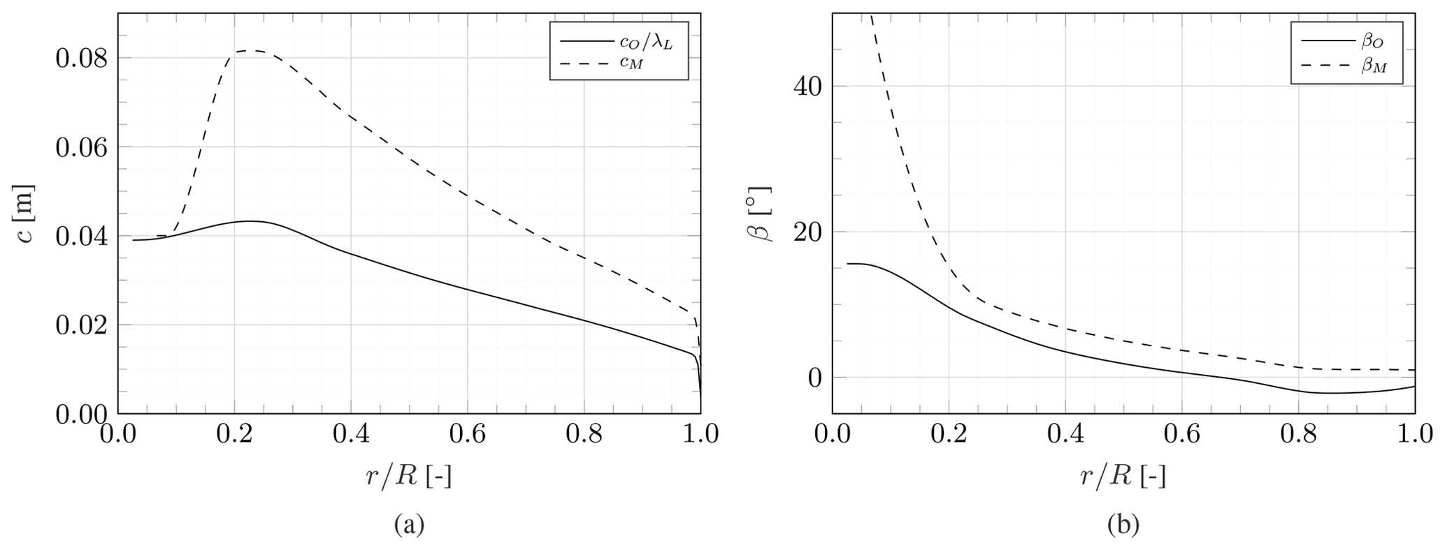
Figure 2Chord (a) and twist (b) distribution of the geometrically scaled IEA 15 MW RWT and the wind tunnel model.
The presented scaling approach ensures close resemblance of the model's non-dimensionalised thrust distribution to that of its reference. It should, however, be noted that other flow physics, such as flow transition or separation, can be fundamentally different due to the changes in airfoil and chord Reynolds number.
2.2 Experimental setup and measurement system
The experiments were conducted in the Open Jet Facility at the TU Delft Faculty of Aerospace Engineering, which is a closed-circuit open jet wind tunnel. The jet exit is an octagon of 2.85 m×2.85 m. The turbine was operated at an approximate tip-speed ratio of λ=9 and an inflow velocity of U∞=3.75 m s−1. To achieve the desired tip-speed ratio, the turbine is driven by a motor that closely maintains the set rotational speed. Inflow conditions of the wind tunnel were logged for each measurement point and showed no significant variation. The wind tunnel was kept at a constant temperature of 20 °C.
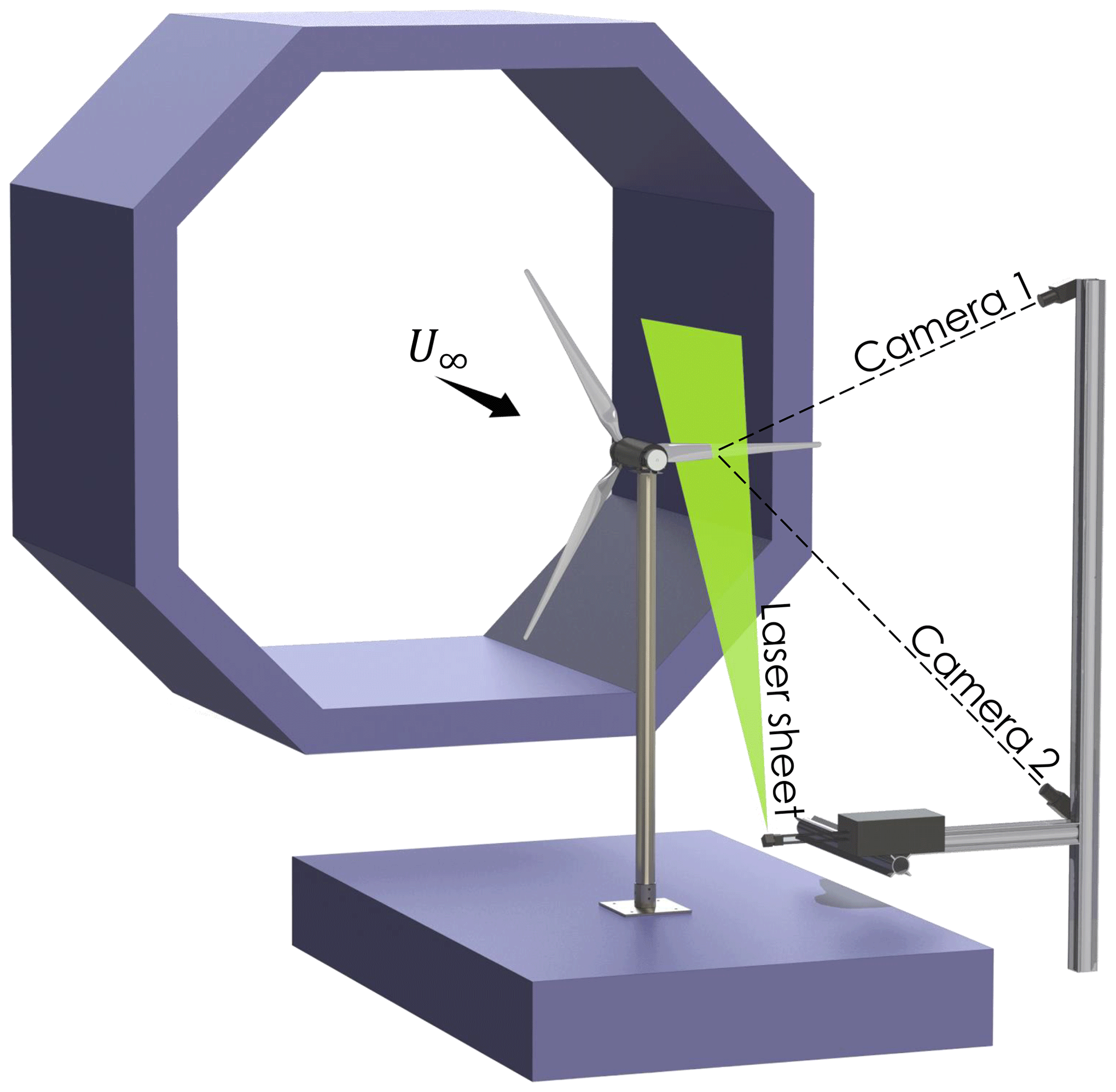
In this campaign, SPIV was used to non-intrusively measure the flow around the blades. A Quantel Evergreen double-pulsed neodymium-doped yttrium aluminium garnet (Nd:YAG) laser provides the light source. Using laser optics, a thin vertical laser sheet was generated that illuminates the area around the targeted blade cross-section. To reduce reflections of the laser, the blades and most other turbine components were spray-painted matt black. A Safex smoke generator produced smoke particles with a median diameter of 1 µm, which were used as tracers. The smoke generator was placed downstream of the tunnel test section, ensuring homogeneous mixing during the flow recirculation.
Two LaVision Imager sCMOS cameras with lenses of 105 mm focal length and an aperture of captured the illuminated particles during the two laser pulses. The laser and cameras were simultaneously triggered by an optical sensor that was activated by a notch in the rotor shaft once per revolution. A time delay between the optical sensor's signal and the laser and camera trigger ensured the blade was in the horizontal position during its upward movement when taking the images. The delay value of 41 ms was determined by comparing images captured during operation with pictures captured during standstill with the blade fixed in the desired horizontal position. This comparison was conducted close to the blade tip where the rotational velocity is highest and thus the position of the cross-section in the field of view most sensitive to the time delay value. The image pairs were taken with a time separation of 150 µs, which allowed the tracing of the particles' movement. This time separation is equivalent to a particle movement of approximately 5 pixels and a turbine rotation of 0.3°. At each measurement location, 120 phase-locked images were taken, which are used in post-processing to obtain an average flow field and its standard deviation. The images are acquired and processed using the LaVision Davis 8 software. The field of view (FOV) resulting from this measurement setup is approximately and the final image resolution is 8.81 pixels mm−1.
Both cameras and laser were mounted rigidly on a traversing system. This way, velocity measurements could be conducted at multiple radial stations without the need to refocus the cameras and calibrate the software. Figure 3 shows a schematic of the measurement setup.
A total of 22 measurement planes were placed along the blade span as follows.
-
for
-
for
-
for
This selection aims at accurately representing the stronger gradients in blade aerodynamics typically present close to the tip. At four radial locations, namely at , measurements were taken for all three blades to evaluate how representative the main measurement blade is for the remaining two blades.
When illuminating a cross-section, the blade casts a shadow where no particles could be traced. Thus, the flow field was captured in two steps. In a first step, the blade's pressure side was evaluated by placing the laser upstream of the turbine and angling the laser sheet downstream. Following that, the laser was relocated downstream of the rotor plane and its laser sheet was tilted upstream to capture the suction side (as shown in Fig. 3). In a post-processing step, the two flow fields averaged individually over the phase-locked upstream and downstream images were stitched together, resulting in the entire flow field around a blade cross-section.
2.3 Deriving blade-level aerodynamics from PIV measurements
This section presents the equations used to derive the distributed blade aerodynamics regarding bound circulation, induction, inflow angle and angle of attack, and blade loads. Based on these quantities, it is possible to calculate the experimental lift polar, too. In this study, the equations presented below are applied under the assumption of local two-dimensional flow; i.e. only the velocity components in the measurement plane are considered.
2.3.1 Determination of bound circulation
The bound circulation Γ at each measurement location can be calculated as the line integral of the measured velocity field u along a curve S enclosing the blade cross-section (e.g. Anderson, 2017, p. 176).
A study of the sensitivity to the bounding curve's size is presented in Appendix A. It revealed that the circulation and also the forces calculated using Noca's method (see Sect. 2.3.3) do not exhibit perfect convergence with varying control volume size. As a consequence, the methods presented in this section are applied for multiple control volumes with different sizes, from which a mean value and standard deviation are calculated.
2.3.2 Determination of induced velocities, inflow angle and angle of attack
Several methods for determining the local inflow conditions exist. The inverse BEM approach (Bruining et al., 1993; Snel et al., 1994; Bak et al., 2006) uses measured and/or simulated forces as input to the blade element momentum equations and iteratively solves for the inflow conditions. Other methods characterise the inflow based on the annulus average flow field (Hansen and Johansen, 2004; Johansen and Sørensen, 2004) or based on the wake induction at the plane exactly between two blades (Herráez et al., 2018). Other approaches use the bound circulation strength to estimate local induced velocity and consequently the inflow conditions (Shen et al., 2007, 2009; Jost et al., 2018). Several benchmarks of these methods have been conducted based on CFD and/or experimental data (Guntur and Sørensen, 2014; Herráez et al., 2018; Rahimi et al., 2018).
The approach denoted as the Ferreira–Micallef method in Rahimi et al. (2018) is used here. It relies on potential flow theory to estimate the induced velocities at each spanwise location. This theory states that the velocity at any point can be expressed by the sum of the relative velocity and the velocities induced by free and bound vorticity such that the measured velocity at a point p is given as
The Biot–Savart law is employed to determine the sum of the induced velocities at a set of control points located along S so that
where xp and x are the position vectors of the control point and inducing vortex element, respectively. By minimising the error between up and uind using a least-squares approach, the relative inflow vector Vrel is determined, yielding the local axial and tangential induction factors.
Knowing the induced velocities, the local inflow angle and angle of attack can then be calculated as
2.3.3 Determination of blade loads
Noca's method. The forces exerted by an immersed body on the surrounding fluid can be evaluated by integrating the change of momentum over a finite control volume. Noca et al. (1999) presented an alternative formulation of the momentum conservation equation, solely relying on surface integrals of flow quantities placed on the boundary of the control volume. The forces can thus be derived from the measured velocity field and its spatial and time derivatives. This approach has been successfully applied to PIV data collected on a vertical-axis wind turbine by LeBlanc and Ferreira (2022). The force per density is given by
where n is the normal vector of the bounding curves, γ is the flux term, S is the outer boundary curve of the control volume surrounding the immersed body, SB is the control volume's inner boundary curve prescribed by the immersed body's surface and uB is the velocity vector of the immersed body's surface.
The term is related to the flow through the inner boundary curve SB. Given the solid airfoil surface, this term is zero. The third term describes the force due to acceleration of the inner boundary surface. As the model wind turbine was running at a constant speed during the experiment, the velocity of the airfoil representing the inner boundary surface can be approximated as constant within the measurement plane. Therefore, this term is zero, too. The flux term γ can be determined as
where I is the identity matrix, 𝒩 is the dimensional constant, ω is the vorticity vector and τ is the Reynolds stress tensor.
There are two possible frames of reference in which to apply the equations given above. On the one hand, a stationary reference frame can be chosen, where the measured blade cross-section moves vertically through the control volume; see Fig. 4a. On the other hand, a reference frame rotating with the investigated cross-section can be used; see Fig. 4b. While the original PIV data are captured in a stationary reference frame, they can easily be converted to a rotating frame by adding the apparent rotational velocity to the measured vertical velocity component v.
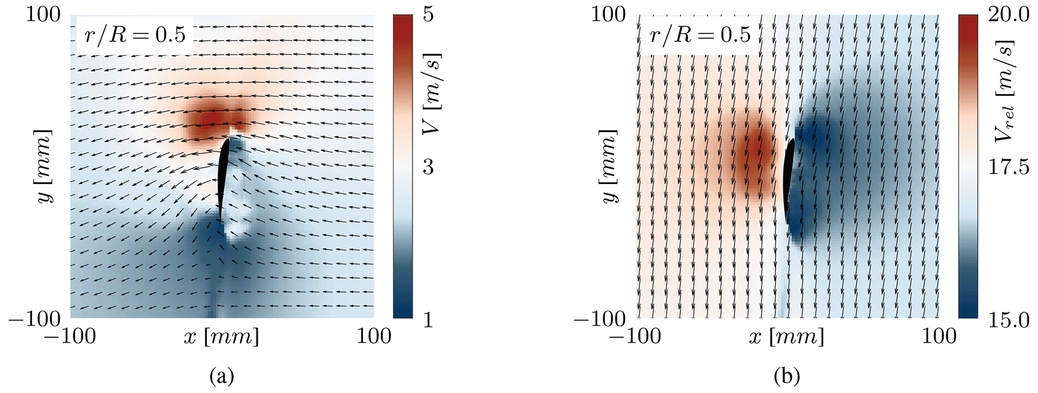
For the analysis performed in the present work, a rotating frame of reference is chosen. In this reference frame, the time derivatives of Eq. (15) are zero.
Kutta–Joukowski theorem (KJ). Alternatively to Noca's method, the forces can be derived from the bound circulation using the Kutta–Joukowski theorem (e.g. Anderson, 2017, p. 282), which states that the sectional lift force is given by L=ρ Vrel Γ. This formulation can be decomposed to yield the forces normal and tangential to the rotor plane.
It should be noted that the Kutta–Joukowski theorem is based on potential flow theory. Thus, e.g. the viscous drag contribution to the tangential force is neglected.
3.1 Determination of the combined pitch and twist offset
The blades used in this experiment are made of vacuum-infused carbon-fibre-reinforced material. This partially manual manufacturing approach led to minor differences between the three blades. Based on visual inspection, one blade was chosen on which the measurement campaign was mainly conducted, hereafter called blade 1. However, measurements were taken for blades 2 and 3 at to estimate the main measurement blade's representation of the other two blades.
Early investigations into the gathered data indicated non-negligible differences in blade aerodynamics between the three blades. To explain this behaviour, the blade cross-sections visible in the raw images were visually inspected and compared against the original design of the blade. This approach is visualised in Fig. 5a, where the blade cross-section is illuminated in white. The original design is overlaid as a red airfoil shape. Then, the correct local twist is found by rotating this airfoil around the trailing edge until its pressure side approximately follows the same curve as the pressure side of the illuminated cross-section. This correction was determined with a precision of 0.1°. The corrected airfoil is shown in green. Based on this comparison, it became apparent that the blade cross-sections were positioned at different angles than designed, resulting in the offset in twist and pitch shown in Fig. 5b.
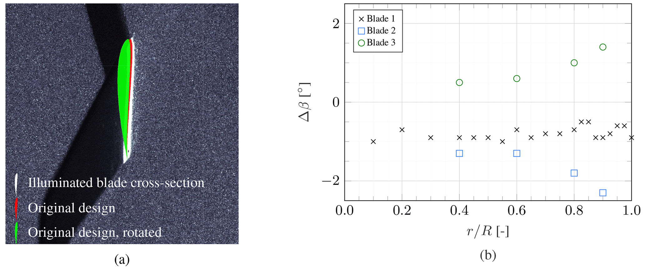
Figure 5Approach of determining actual local airfoil orientation (a), as well as the twist and pitch offset determined by comparing experimentally captured blade cross-sections to the original design (b).
For blade 1, where many data points are available along the span, a quadratic fit is used to describe the trend and balance out the fluctuations likely due to human error in the interpretation of the raw images. Blade 1 appears to have a pitch offset of approximately −1 ° and additionally shows slight twist deformation towards the tip. More extreme twist deformations can be observed for blades 2 and 3, with opposite directions. This shows how challenging the use of vacuum-infused carbon-fibre composite blades is. Despite having the same fibre lay-up, the manufacturing process is a highly manual task where minor differences can impact the structural properties of the blade. The pitch offset can be explained by the model turbine's connection between blade root and hub: the turbine is equipped with a manual pitch mechanism which is fixed in the desired position using set screws. Despite being used with care, this manual mechanism is likely the origin of the pitch deviations between the three blades. As these deviations from the intended design were only found in post-processing after the campaign had ended, no correction to the pitch angle could be made.
3.2 Flow field
The flow fields represent the primary data collected during this experiment using stereoscopic PIV. Figure 6 depicts the measured velocity magnitude fields at the four radial stations where data for all three blades are available. Overall, the general flow patterns are in good agreement. However, the twist and pitch offset described in the previous section leads to differences in the angle of attack, explaining minor discrepancies in velocity magnitudes. For example, blade 2, exhibiting twist deformations towards higher angles of attack, induces higher velocities, while the opposite holds for blade 3.
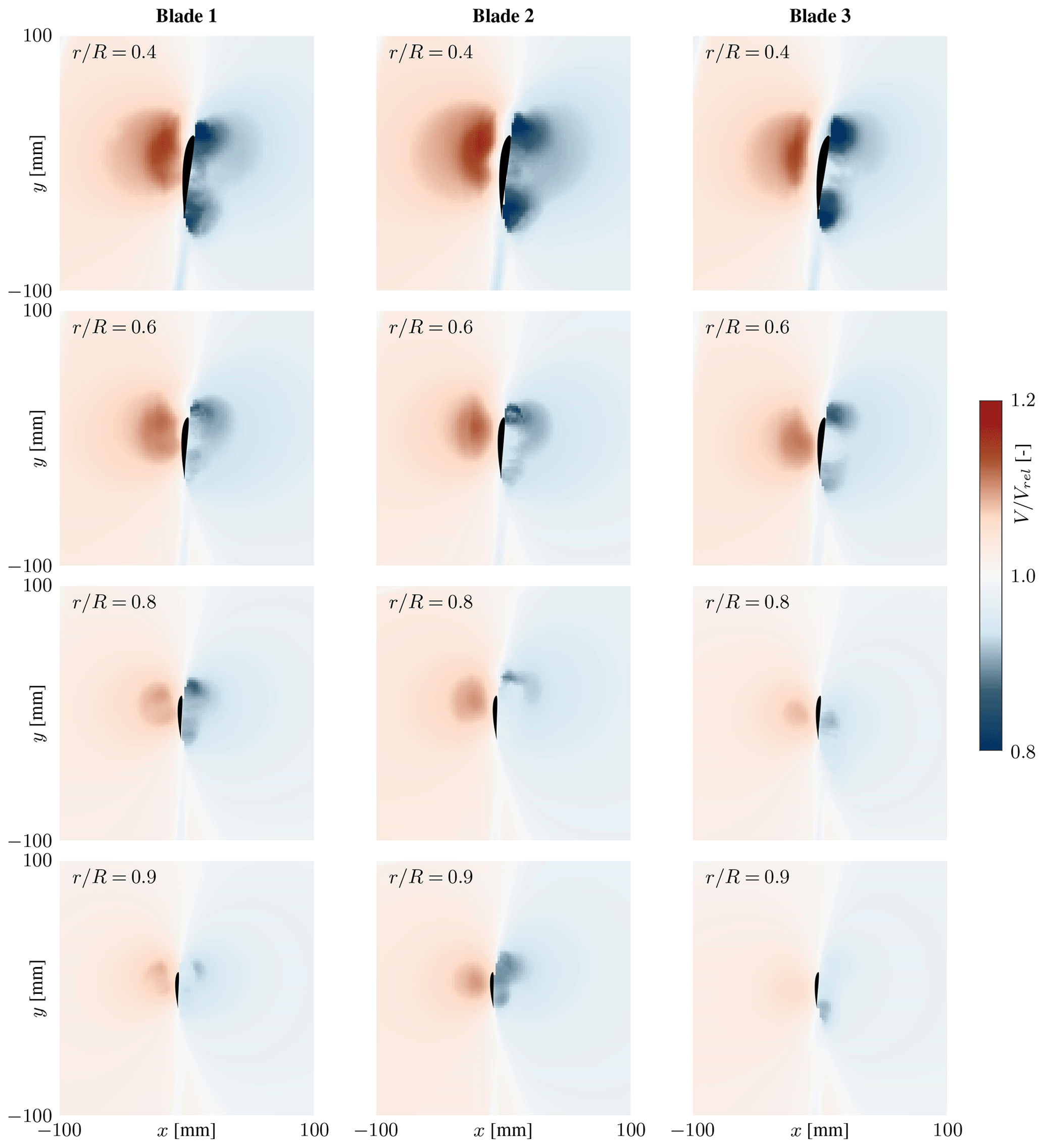
Figure 6Non-dimensionalised velocity magnitudes at the radial stations measured for all three blades.
Notably, many measurement points have low-velocity regions close to the suction side surface. Here, laser reflections from the blade surface reduce the accuracy of the PIV processing. This is less the case on the pressure side, where the concave blade surface causes lower reflections.
3.3 Blade aerodynamics
All plots presented in this section contain error bars. These represent the 95 % confidence interval and are based on variations in the measured velocity field during the capturing of the PIV images as well as in the processing with various control volume sizes; see Appendix A. This uncertainty is a measure of both the quality of the phase lock and the unsteadiness of the flow. While almost all data points have very low uncertainty, the measurement point closest to the root suffers from the laser reflecting off the nacelle and hub, increasing measurement uncertainty. This effect is visible to a varying degree in all derived aerodynamic quantities.
Figure 7 shows the circulation distribution of the three blades. The effect of varying pitch angles and twist deflection expresses itself in the different circulation levels of the three individual blades.
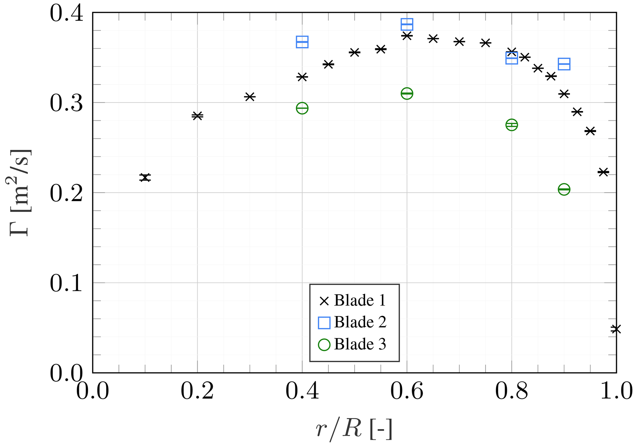
Figure 7Spanwise distribution of bound circulation, with error bars representing the 95 % confidence interval.
The axial and tangential induction factor distribution is shown in Fig. 8. Compared to the circulation distribution, differences in induction are minor between the three blades. This is a significant finding in support of fundamental BEM theory, which uses a rotor-averaged induction factor.
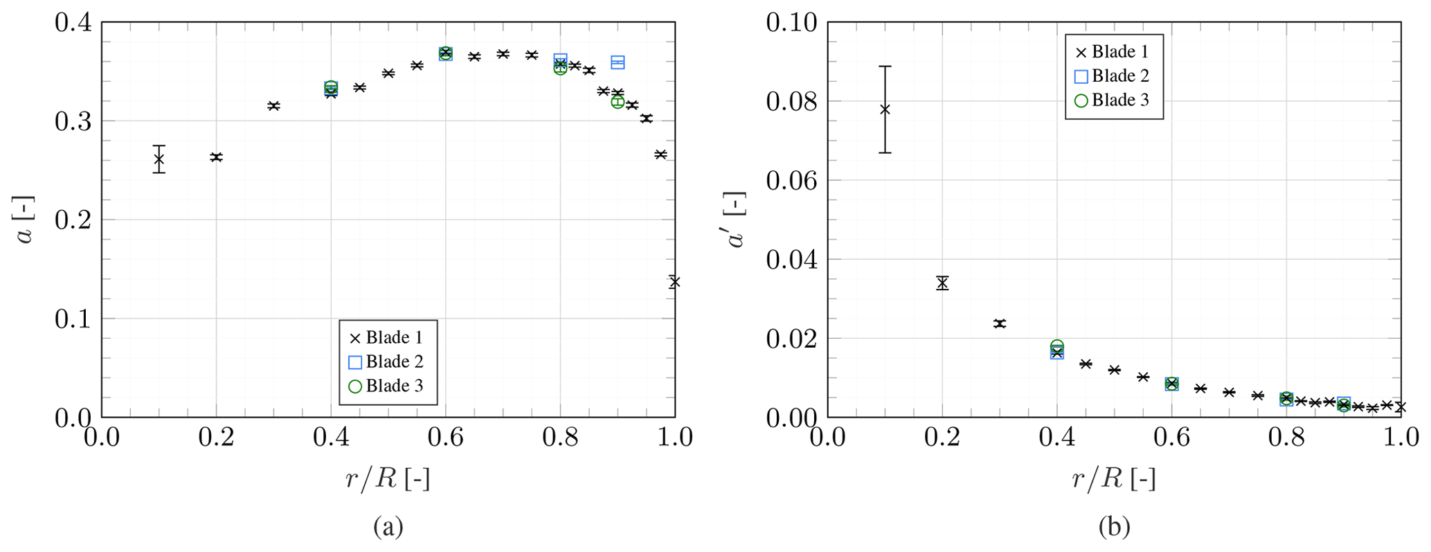
Figure 8Spanwise distribution of axial (a) and tangential (b) induction factors, with error bars representing the 95 % confidence interval.
Figure 9 depicts the local inflow angle and angle of attack distribution. Given that the blades have a cylindrical cross-section at , the value of the angle of attack at this location is meaningless and reported for completeness only. The angle of attack distribution is evidently influenced by the pitch and twist variations between the three blades. Despite these variations, all derived angles of attack are well within the linear region of the design airfoil's lift polar.
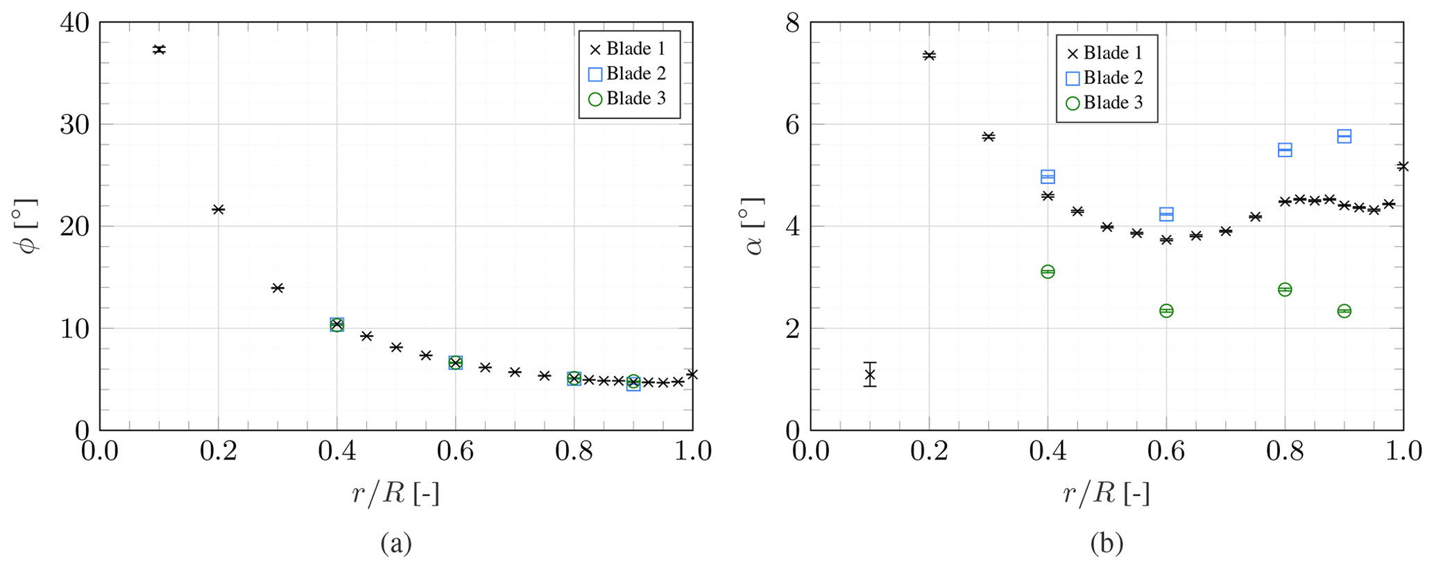
Figure 9Spanwise distribution of inflow angle (a) and angle of attack (b), with error bars representing the 95 % confidence interval.
The axial and tangential force distributions are presented in Fig. 10. Two methods are employed to derive the normal force distribution, namely Noca's method and the Kutta–Joukowski (KJ) theorem. Both methods are in close agreement; a linear fit between the results of all three blades yields with R2=0.9965. By integrating the normal force distribution, the rotor thrust can be calculated and non-dimensionalised to obtain the thrust coefficient. To this end, piecewise cubic curves are fit to the experimental results. Where no data are available at blade root and tip, zero loading is assumed. The resulting thrust coefficients are and . For a tip-speed ratio of λ=9, the IEA 15 MW RWT has a thrust coefficient of CT=0.8 (Gaertner et al., 2020). Thus, the relative deviation of the thrust-scaled blades to their reference corresponds to % and %, respectively.
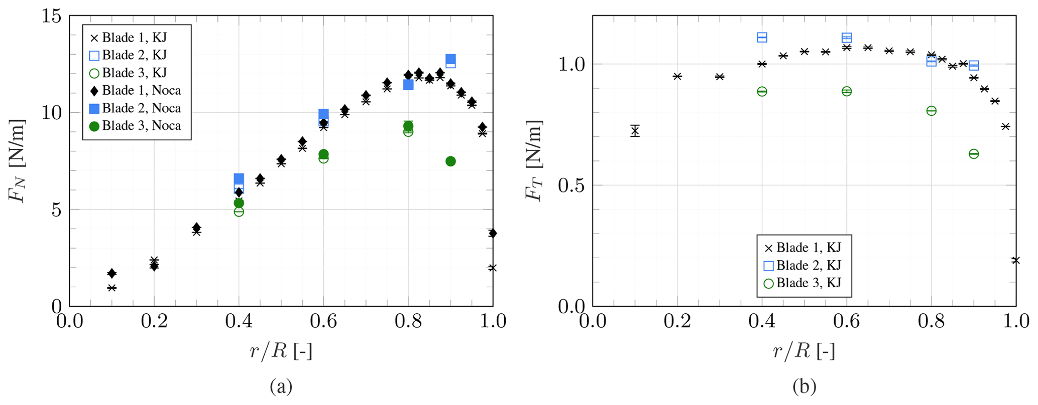
Figure 10Spanwise distribution of normal (a) and tangential (b) force, with error bars representing the 95% confidence interval.
As demonstrated in Appendix A, Noca's method is, however, unreliable when estimating the tangential force from this experimental dataset. Therefore, only the tangential force derived using the Kutta–Joukowski theorem is presented here. It is noteworthy that this method neglects viscous effects and consequently misses the contribution of the viscous drag. Overall, the normal and tangential force trends are consistent between the three blades. However, the magnitude is fairly different, with blade 2 having, on average, slightly higher values than blade 1, while blade 3 exhibits lower values than the other two blades. These differences are in line with the pitch and twist offset discussed in Sect. 3.1.
3.4 Lift polar
Based on the aerodynamic quantities presented in the previous section, the lift coefficient is derived. The lift force is calculated using the force distributions based on the Kutta–Joukowski theorem.
Figure 11a shows the experimental lift polar compared to the SD7032 airfoil (Fontanella et al., 2021b) at Reynolds numbers resembling those present in this experiment, which vary between approximately 40 000 and 65 000 depending on the radial position. For clarity, only the mean values are reported. The two measurements closest to the root are omitted as these cross-sections are defined by a cylinder and a blend between a cylinder and the SD7032 airfoil. Additionally, the two measurements closest to the tip are omitted because the tip vortex causes highly three-dimensional flow features, which should not be compared to two-dimensional airfoil polars. The remaining measurement points are in good agreement with the lift coefficient curve of the design airfoil.
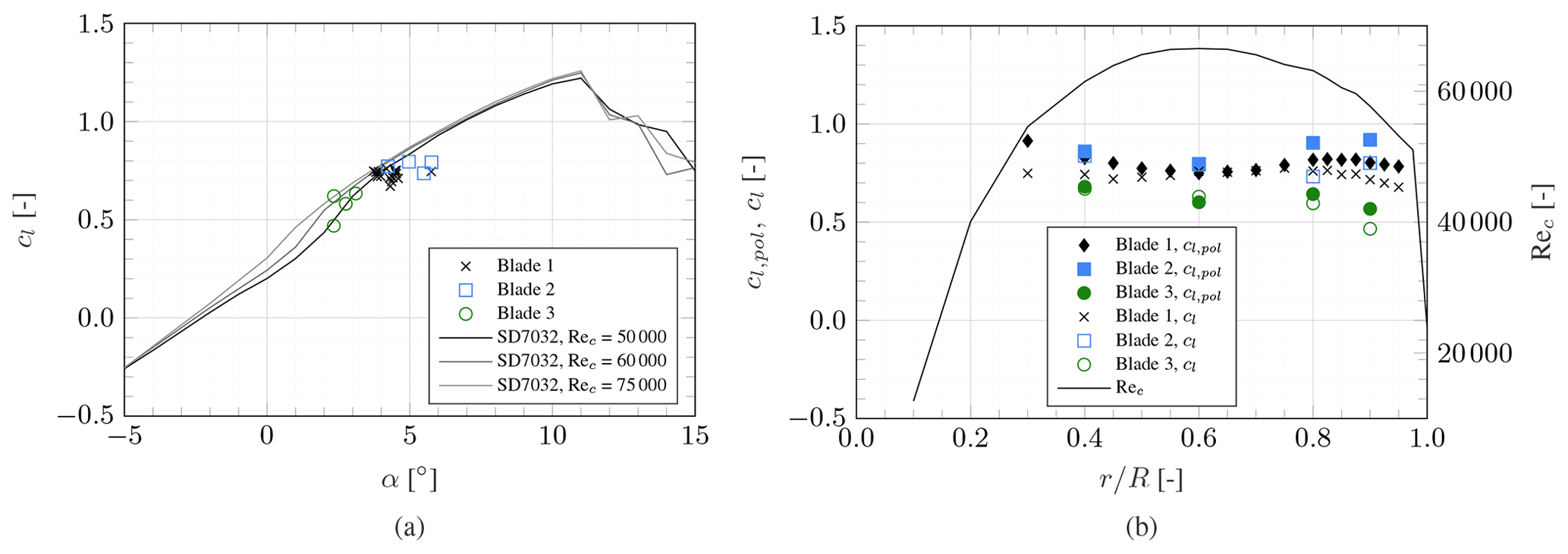
Figure 11Experimental lift polar compared to the SD7032 airfoil lift polar (a) and comparison between the lift coefficient derived from measured forces to that expected based on the design lift polars, alongside the chord Reynolds number distribution (b).
While giving an indication of the experimentally derived lift polar, Fig. 11a does not represent the variable Reynolds number along the blade. Alternatively, the design airfoil polars can be interpolated for the experimentally derived Reynolds number and angle of attack to obtain a polar-based, expected lift coefficient cl,pol. These values are plotted alongside the lift coefficient based on the measured forces and the spanwise distribution of the chord Reynolds number in Fig. 11b. It demonstrates that, in the root and tip region, the blades used in this experiment produce less lift than would be expected. It can be hypothesised that this is a consequence of differences in surface finish between the used blades and the airfoil measured by Fontanella et al. (2021a), as well as minor inaccuracies in the manually produced geometry.
This study presents the results from an experimental campaign on a thrust-scaled version of the IEA 15 MW RWT. Particle image velocimetry is used to measure the flow field at multiple radial stations around the blade. Various aerodynamic blade properties are derived directly from the measured flow field along a closed curve around the blade cross-sections: the circulation is determined from the velocity integral, the inflow conditions by removing the blade induction from the measured flow field using elemental potential flow solutions, and the forces based on Noca's method and the Kutta–Joukowski theorem.
Early analyses revealed that the blades were mounted with minor deviations from the desired pitch angle and, on top of that, exhibited twist deformations. This leads to considerable differences in the angle of attack and consequently blade loads among the three blades, which is consistently reflected in their experimentally derived spanwise distributions. In contrast, the derived induction values remain nearly constant between the three blades, indicating that induction can be considered a rotor-averaged phenomenon. This is an experimental confirmation of one of the fundamental assumptions in blade element momentum theory.
The dataset created in this wind tunnel experiment fully characterises the three blades in terms of the surrounding flow field, bound circulation, local inflow conditions and blade loads. The normal force distributions derived using Noca's method and the Kutta–Joukowski theorem were found to be in good agreement. Knowing these aerodynamic parameters, it can be demonstrated that the lift coefficient measured along the span follows the trend of the lift polar used in the blade design. There are, however, slight deficits in lift production in the root and tip regions compared to the expected values based on the design airfoil's lift polar.
The experimental data presented here can be used in future numeric model validation studies. It provides data relevant for validating low-fidelity models, such as algorithms based on blade element momentum theory or lifting line theory, and for mid- to high-fidelity models, such as panel codes and computational fluid dynamics. Since the model blade is based on the IEA 15 MW RWT, the non-dimensionalised loads resemble the current state of the art of real offshore wind turbines and numerical reference models. Furthermore, the newly created model wind turbine can be used in future experiments investigating the aerodynamics of this reference wind turbine.
To reduce the impact of blade deformations in future research, it is recommended to either produce a new set of blades with less variation in their stiffness properties or to apply more advanced deformation tracking techniques such as photogrammetry. To improve the accuracy in pitch setting, the manual pitch mechanism could be exchanged for a variable pitch mechanism controlled by a motor. This would then require an initial calibration before a new experimental campaign.
In this study, the blade's aerodynamic quantities are determined by interrogating flow information along a closed curve enclosing the investigated blade cross-section. A circular curve is chosen with the blade cross-section positioned in its centre. To verify the methods presented in Sect. 2.3, a panel code developed by Ribeiro et al. (2022) based on the work of Katz and Plotkin (2001) is used to replicate the wind tunnel experiment numerically. The panel code simulates the three-dimensional surface of the blade and can be used to derive flow fields at locations equivalent to the measurement planes of the experiment. Such results then offer the opportunity to derive circulation and loads based on the velocity field around the blade (“indirect”) but also from the aerodynamic solution on the blade (“direct”). By comparing these two approaches, the methods for deriving aerodynamic quantities from the flow field can be verified before applying them to the experimental data.
Figure A1 shows the sensitivity of the calculated circulation and of the forces based on Noca's method to the control volume's size, given as the ratio of its radius rCV to the local chord, at three radial locations. When calculating the forces based on the Kutta–Joukowski theorem, they are directly proportional to the circulation distribution and are thus not presented here.
The sensitivity is investigated for both the experimental data and the panel code results. Generally, there is a conflict of interest between the data points per control volume size, which favours a large control volume, and the approximation of two-dimensional flow in a flat measurement surface, which favours a small control volume.
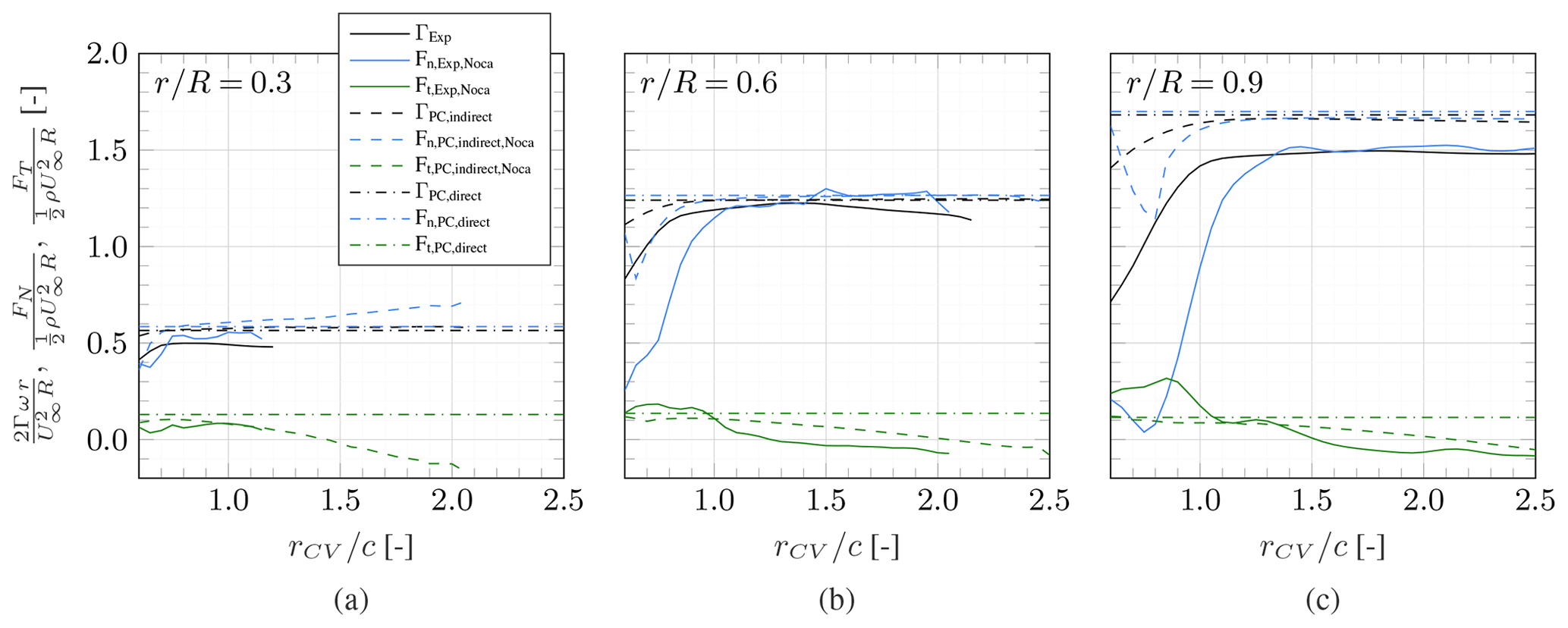
Figure A1Sensitivity of determined blade loads and circulation to the chosen boundary curve size at various radial stations.
For the panel code (PC) results, it can be observed that the indirectly determined circulation converges against the directly determined value with increasing control volume size. For the normal force, this is only true for the two outboard sections shown in Fig. A1b and c. The discrepancy between the direct and indirect approach at the inboard section can be attributed to the increasing flow curvature in this region, which stands in contrast to the two-dimensional control volume.
In contrast to circulation and normal force, the tangential force does not converge anywhere along the span but rather decreases with increasing control volume size. The high tip-speed ratio of the model turbine entails very low torque values and the tangential force is very small. As such, the momentum change corresponding to the tangential force is difficult to capture with the Noca method. Based on this finding, only the tangential force calculated via the Kutta–Joukowski theorem is presented in this article.
The circulation and forces determined based on the experimental data largely follow the same trends observed for the panel code results. However, given the less clean flow field, the convergence is not as steady and shows slight deviations even after the initial, clearly unconverged, ramp. This is particularly true for the forces calculated using Noca's method, which relies on sensitive derivatives of the velocity field. To limit the influence of the control volume, the convergence is evaluated individually for each measurement plane and the endpoint of the initial convergence ramp is identified. The aerodynamic quantities are determined for multiple control volumes with sizes beyond the initial convergence ramp and then averaged over these. This approach yields the results presented in Sect. 3.3. It should further be noted that for the experimental results, the largest possible control volume is dictated by the available field of view. Thus, the convergence of methods such as Noca's should be taken into consideration when defining the PIV setup and consequently the field of view.
| Latin letters | |
| Axial and tangential induction factor | |
| Cc | Chord scaling constant |
| CT | Thrust coefficient |
| c | Chord |
| cl, cd | Lift and drag coefficient |
| Lift coefficient at zero angle of attack | |
| D | Rotor diameter, drag force |
| Droot | Diameter of the blade root section |
| F | Force vector |
| FN, FT | Normal and tangential force |
| I | Identity matrix |
| Kl | Lift slope |
| L | Lift force |
| 𝒩 | Dimensional constant |
| n | Normal vector |
| R | Blade tip radius |
| Rec | Chord Reynolds number |
| r | Radial coordinate |
| rroot | Blade root radius |
| S, SB | Outer- and inner boundary curve of a control volume |
| t | Time |
| U∞ | Freestream velocity |
| u | Velocity vector |
| u, v | Velocity components |
| Vrel | Relative inflow velocity |
| Vrot | Rotational velocity |
| x | Position vector |
| Greek letters and other symbols | |
| α | Angle of attack |
| β | Blade twist angle |
| Γ | Circulation |
| γ | Flux term |
| λ | Tip-speed ratio |
| λL | Geometric scaling factor |
| ρ | Density of air |
| τ | Reynolds stress tensor |
| ϕ | Inflow angle |
| ω | Angular velocity |
| ω | Vorticity vector |
| ∇ | Nabla operator |
| Subscripts | |
| CV | Control volume |
| ind | Induced |
| KJ | Kutta–Joukowski |
| M | Model |
| O | Original |
| pol | Based on design polars |
The data presented in this study, as well as information regarding the blade planform and logged wind tunnel operating conditions, are openly available on the 4TU.ResearchData repository at https://doi.org/10.4121/164890ab-39d7-4af8-8b3c-9e21f789b80a (Fritz et al., 2024).
EF designed the wind turbine model, built the model blades, planned and executed the experiment, and post-processed and analysed the measurement data. AR contributed to the experiment execution and data analysis and provided numerical simulations to help the development of post-processing methods. KB acquired funding and contributed to the experiment planning and the data analysis. CF acquired funding and contributed to the experiment planning and execution, the development of post-processing methods, and the data analysis.
The contact author has declared that none of the authors has any competing interests.
Publisher’s note: Copernicus Publications remains neutral with regard to jurisdictional claims made in the text, published maps, institutional affiliations, or any other geographical representation in this paper. While Copernicus Publications makes every effort to include appropriate place names, the final responsibility lies with the authors.
This contribution has been financed with Topsector Energiesubsidie from the Dutch Ministry of Economic Affairs under grant no. TEHE119018. The wind tunnel experiment was financed by internal TU Delft funding.
This paper was edited by Jonathan Whale and reviewed by two anonymous referees.
Akay, B., Ragni, D., Ferreira, C. S., and van Bussel, G.: Experimental investigation of the root flow in a horizontal axis wind turbine, Wind Energy, 17, 1093–1109, https://doi.org/10.1002/we.1620, 2013. a
Allen, C., Viscelli, A., Dagher, H., Goupee, A., Gaertner, E., Abbas, N., Hall, M., and Barter, G.: Definition of the UMaine VolturnUS-S Reference Platform Developed for the IEA Wind 15-Megawatt Offshore Reference Wind Turbine, Tech. Rep. NREL/TP-5000-76773, National Renewable Energy Lab. (NREL), Golden, CO (United States), Univ. of Maine, Orono, ME (United States), https://doi.org/10.2172/1660012, 2020. a
Anderson, J. D.: Fundamentals of aerodynamics, McGraw-Hill series in aeronautical and aerospace engineering, McGraw-Hill Education, New York, NY, sixth edn., ISBN 978-1-259-12991-9, 2017. a, b
Bak, C., Johansen, J., and Andersen, P. B.: Three-dimensional corrections of airfoil characteristics based on pressure distributions, in: Proceedings of the european wind energy conference, 1–10, 2006. a
Bak, C., Zahle, F., Bitsche, R., Kim, T., Yde, A., Henriksen, L. C., Hansen, M. H., Blasques, J. P. A. A., Gaunaa, M., and Natarajan, A.: The DTU 10-MW Reference Wind Turbine, in: Danish Wind Power Research 2013, https://orbit.dtu.dk/files/55645274/The_DTU_10MW_Reference_Turbine_Christian_Bak.pdf (last access: 15 May 2024), 2013. a
Bayati, I., Belloli, M., Bernini, L., and Zasso, A.: Aerodynamic design methodology for wind tunnel tests of wind turbine rotors, J. Wind Eng. Ind. Aerod., 167, 217–227, https://doi.org/10.1016/j.jweia.2017.05.004, 2017. a, b
Berger, F., Kröger, L., Onnen, D., Petrović, V., and Kühn, M.: Scaled wind turbine setup in a turbulent wind tunnel, J. Phys. Conf. Ser., 1104, 012026, https://doi.org/10.1088/1742-6596/1104/1/012026, 2018. a
Berger, F., Onnen, D., Schepers, G., and Kühn, M.: Experimental analysis of radially resolved dynamic inflow effects due to pitch steps, Wind Energ. Sci., 6, 1341–1361, https://doi.org/10.5194/wes-6-1341-2021, 2021. a
Boorsma, K. and Schepers, J.: Description of experimental set-up. Mexico measurements, Tech. Rep. ECN-X-09-0XX, Energy Research Center of the Netherlands, 2009. a
Boorsma, K. and Schepers, J.: Description of experimental setup, New Mexico experiment, technical report Tech. Rep. ECN-X15-093 ECN, 2015. a
Bruining, A., Van Bussel, G., Corten, G., and Timmer, W.: Pressure distribution from a wind turbine blade; field measurements compared to 2-Dimensional wind tunnel data, Institute for Windenergy, Delft University of Technology, 1993. a
Butterfield, C., Musial, W., and Simms, D.: Combined experiment phase 1. Final report, Tech. Rep. NREL/TP-257-4655, Office of Scientific and Technical Information (OSTI), https://doi.org/10.2172/10105837, 1992. a
Cho, T. and Kim, C.: Wind tunnel test results for a 2/4.5 scale MEXICO rotor, Renew. Energ., 42, 152–156, https://doi.org/10.1016/j.renene.2011.08.031, 2012. a
Cho, T. and Kim, C.: Wind tunnel test for the NREL phase VI rotor with 2 m diameter, Renew. Energ., 65, 265–274, https://doi.org/10.1016/j.renene.2013.10.009, 2014. a
del Campo, V., Ragni, D., Micallef, D., Akay, B., Diez, F. J., and Simão Ferreira, C.: 3D load estimation on a horizontal axis wind turbine using SPIV, Wind Energy, 17, 1645–1657, https://doi.org/10.1002/we.1658, 2014. a
del Campo, V., Ragni, D., Micallef, D., Diez, F. J., and Ferreira, C. J. S.: Estimation of loads on a horizontal axis wind turbine operating in yawed flow conditions, Wind Energy, 18, 1875–1891, https://doi.org/10.1002/we.1794, 2015. a
Fontanella, A., Bayati, I., Mikkelsen, R., Belloli, M., and Zasso, A.: UNAFLOW: a holistic wind tunnel experiment about the aerodynamic response of floating wind turbines under imposed surge motion, Wind Energ. Sci., 6, 1169–1190, https://doi.org/10.5194/wes-6-1169-2021, 2021a. a, b
Fontanella, A., Bayati, I., Mikkelsen, R., Belloli, M., and Zasso, A.: UNAFLOW: UNsteady Aerodynamics of FLOating Wind turbines, Zenodo [data set], https://doi.org/10.5281/zenodo.4740006, 2021b. a, b, c
Fontanella, A., Facchinetti, A., Di Carlo, S., and Belloli, M.: Wind tunnel investigation of the aerodynamic response of two 15 MW floating wind turbines, Wind Energ. Sci., 7, 1711–1729, https://doi.org/10.5194/wes-7-1711-2022, 2022. a, b, c
Fritz, E. K., Ferreira, C., and Boorsma, K.: An efficient blade sweep correction model for blade element momentum theory, Wind Energy, 25, 1977–1994, https://doi.org/10.1002/we.2778, 2022. a
Fritz, E., Ribeiro, A., Boorsma, K., and Ferreira, C.: Supporting data belonging to the publication Aerodynamic characterisation of a thrust-scaled IEA 15 MW wind turbine model: Experimental insights using PIV data, 4TU.ResearchData [data set], https://doi.org/10.4121/164890ab-39d7-4af8-8b3c-9e21f789b80a, 2024. a
Gaertner, E., Rinker, J., Sethuraman, L., Zahle, F., Anderson, B., Barter, G., Abbas, N., Meng, F., Bortolotti, P., Skrzypinski, W., Scott, G., Feil, R., Bredmose, H., Dykes, K., Shields, M., Allen, C., and Viselli, A.: Definition of the IEA wind 15-megawatt offshore reference wind turbine Tech. Rep. NREL/TP-5000-75698, https://www.nrel.gov/docs/fy20osti/75698.pdf (last access: 14 May 2024), 2020. a, b, c
Grasso, F., van Garrel, A., and Schepers, G.: Development and validation of generalized lifting line based code for wind turbine aerodynamics, in: 49th AIAA aerospace sciences meeting including the new horizons forum and aerospace exposition, American Institute of Aeronautics and Astronautics, 146–164, https://doi.org/10.2514/6.2011-146, 2011. a
Guntur, S. and Sørensen, N. N.: An evaluation of several methods of determining the local angle of attack on wind turbine blades, J. Phys.-Conf. Ser., 555, 012045, https://doi.org/10.1088/1742-6596/555/1/012045, 2014. a
Hand, M. M., Simms, D. A., Fingersh, L. J., Jager, D. W., Cotrell, J. R., Schreck, S., and Larwood, S. M.: Unsteady aerodynamics experiment phase VI: Wind tunnel test configurations and available data campaigns, Tech. Rep. NREL/TP-500-29955, Office of Scientific and Technical Information (OSTI), https://doi.org/10.2172/15000240, 2001. a
Hansen, M. O. L. and Johansen, J.: Tip studies using CFD and comparison with tip loss models, Wind Energy, 7, 343–356, https://doi.org/10.1002/we.126, 2004. a
Herráez, I., Daniele, E., and Schepers, J. G.: Extraction of the wake induction and angle of attack on rotating wind turbine blades from PIV and CFD results, Wind Energ. Sci., 3, 1–9, https://doi.org/10.5194/wes-3-1-2018, 2018. a, b
Johansen, J. and Sørensen, N. N.: Aerofoil characteristics from 3D CFD rotor computations, Wind Energy, 7, 283–294, https://doi.org/10.1002/we.127, 2004. a
Jonkman, J., Butterfield, S., Musial, W., and Scott, G.: Definition of a 5-MW Reference Wind Turbine for Offshore System Development, Tech. Rep. NREL/TP-500-38060, 947422, https://doi.org/10.2172/947422, 2009. a
Jost, E., Klein, L., Leipprand, H., Lutz, T., and Krämer, E.: Extracting the angle of attack on rotor blades from CFD simulations, Wind Energy, 21, 807–822, https://doi.org/10.1002/we.2196, 2018. a
Katz, J. and Plotkin, A.: Low-speed aerodynamics, Cambridge University Press, https://doi.org/10.1017/cbo9780511810329, 2001. a
Kimball, R., Robertson, A., Fowler, M., Mendoza, N., Wright, A., Goupee, A., Lenfest, E., and Parker, A.: Results from the FOCAL experiment campaign 1: turbine control co-design, J. Phys. Conf. Ser., 2265, 022082, https://doi.org/10.1088/1742-6596/2265/2/022082, 2022. a, b
Langidis, A., Nietiedt, S., Berger, F., Kröger, L., Petrović, V., Wester, T. T. B., Gülker, G., Göring, M., Rofallski, R., Luhmann, T., and Kühn, M.: Design and evaluation of rotor blades for fluid structure interaction studies in wind tunnel conditions, J. Phys. Conf. Ser., 2265, 022079, https://doi.org/10.1088/1742-6596/2265/2/022079, 2022. a
LeBlanc, B. and Ferreira, C.: Estimation of blade loads for a variable pitch vertical axis wind turbine from particle image velocimetry, Wind Energy, 25, 313–332, https://doi.org/10.1002/we.2674, 2022. a
Lignarolo, L., Ragni, D., Krishnaswami, C., Chen, Q., Ferreira, C. S., and van Bussel, G.: Experimental analysis of the wake of a horizontal-axis wind-turbine model, Renew. Energ., 70, 31–46, https://doi.org/10.1016/j.renene.2014.01.020, 2014. a
Micallef, D., Akay, B., Ferreira, C. S., Sant, T., and van Bussel, G.: The origins of a wind turbine tip vortex, J. Phys. Conf. Ser., 555, 012074, https://doi.org/10.1088/1742-6596/555/1/012074, 2014. a
Micallef, D., Ferreira, C. S., Sant, T., and van Bussel, G.: Experimental and numerical investigation of tip vortex generation and evolution on horizontal axis wind turbines, Wind Energy, 19, 1485–1501, https://doi.org/10.1002/we.1932, 2015. a
Muggiasca, S., Taruffi, F., Fontanella, A., Di Carlo, S., and Belloli, M.: Aerodynamic and Structural Strategies for the Rotor Design of a Wind Turbine Scaled Model, Energies, 14, 2119, https://doi.org/10.3390/en14082119, 2021. a
Nietiedt, S., Wester, T. T. B., Langidis, A., Kröger, L., Rofallski, R., Göring, M., Kühn, M., Gülker, G., and Luhmann, T.: A Wind Tunnel Setup for Fluid-Structure Interaction Measurements Using Optical Methods, Sensors, 22, 5014, https://doi.org/10.3390/s22135014, 2022. a
Noca, F., Shiels, D., and Jeon, D.: A comparison of methods for evaluating time-dependant fluid dynamic forces on bodies, using only velocity fields and their derivatives, J. Fluid. Struct., 13, 551–578, https://doi.org/10.1006/jfls.1999.0219, 1999. a
Phengpom, T., Kamada, Y., Maeda, T., Murata, J., Nishimura, S., and Matsuno, T.: Study on blade surface flow around wind turbine by using LDV measurements, J. Therm. Sci., 24, 131–139, https://doi.org/10.1007/s11630-015-0765-3, 2015a. a
Phengpom, T., Kamada, Y., Maeda, T., Murata, J., Nishimura, S., and Matsuno, T.: Experimental investigation of the three-dimensional flow field in the vicinity of a rotating blade, Journal of Fluid Science and Technology, 10, JFST0013, https://doi.org/10.1299/jfst.2015jfst0013, 2015b. a
Phengpom, T., Kamada, Y., Maeda, T., Matsuno, T., and Sugimoto, N.: Analysis of wind turbine pressure distribution and 3D flows visualization on rotating condition, IOSR Journal of engineering, 6, 18–30, 2016. a
Rahimi, H., Schepers, J., Shen, W., García, N. R., Schneider, M., Micallef, D., Ferreira, C. S., Jost, E., Klein, L., and Herráez, I.: Evaluation of different methods for determining the angle of attack on wind turbine blades with CFD results under axial inflow conditions, Renew. Energ., 125, 866–876, https://doi.org/10.1016/j.renene.2018.03.018, 2018. a, b
Ribeiro, A., Casalino, D., and Ferreira, C.: Surging wind turbine simulations with a free wake panel method, J. Phys. Conf. Ser., 2265, 042027, https://doi.org/10.1088/1742-6596/2265/4/042027, 2022. a
Schepers, J. and Snel, H.: Model experiments in controlled conditions, final report, Tech. Rep. ECN-E-07-042, Energy Research Center of the Netherlands, https://publications.tno.nl/publication/34628817/8d6E4g/e07042.pdf (last access: 14 May 2024), 2007. a
Schepers, J. G., Boorsma, K., Cho, T., Gomez-Iradi, S., Schaffarczyk, P., Shen, W. Z., Lutz, T., Stoevesandt, B., Schreck, S., and Micallef, D.: Analysis of mexico wind tunnel measurements. Final report of IEA task 29, mexnext (phase 1), https://publications.tno.nl/publication/34629143/5lE9u6/e12004.pdf (last access: 14 May 2024), 2012. a
Schepers, J. G. and Schreck, S. J.: Aerodynamic measurements on wind turbines, Wires Energy Environ., 8, e320, https://doi.org/10.1002/wene.320, 2018. a
Shen, W. Z., Hansen, M. O. L., and Sørensen, J. N.: Determination of angle of attack (AOA) for rotating blades, in: Wind energy, Springer, Berlin, Heidelberg, 205–209, https://doi.org/10.1007/978-3-540-33866-6_37, 2007. a
Shen, W. Z., Hansen, M. O. L., and Sørensen, J. N.: Determination of the angle of attack on rotor blades, Wind Energy, 12, 91–98, https://doi.org/10.1002/we.277, 2009. a
Simms, D. A., Hand, M. M., Fingersh, L. J., and Jager, D. W.: Unsteady aerodynamics experiment phases II-IV test configurations and available data campaigns, Tech. Rep. NREL/TP-500-25950, Office of Scientific and Technical Information (OSTI), https://doi.org/10.2172/12144, 1999. a
Snel, H., Houwink, R., and Bosscher, T.: Sectional prediction of lift coefficients on rotating wind turbine blades in stall, netherlands, Tech. Rep. ECN-C-93-052, Energy Research Center of the Netherlands, 1994. a
Taruffi, F., Novais, F., and Viré, A.: An experimental study on the aerodynamic loads of a floating offshore wind turbine under imposed motions, Wind Energ. Sci., 9, 343–358, https://doi.org/10.5194/wes-9-343-2024, 2024. a
Xiao, J.-p., Wu, J., Chen, L., and Shi, Z.-y.: Particle image velocimetry (PIV) measurements of tip vortex wake structure of wind turbine, Appl. Math. Mech., 32, 729–738, https://doi.org/10.1007/s10483-011-1452-x, 2011. a