Validation of aeroelastic dynamic model of active trailing edge flap system tested on a 4.3 MW wind turbine

Active trailing edge flap (ATEF) is a promising technology for controlling wind turbine loads and enhancing energy production. The integration of this technology in the design of commercial wind turbines requires dedicated flap aeroelastic models, as aeroelastic simulations have an essential role in the wind turbine design process. Several aeroelastic codes developed specific flap modules. However, these models were only partially validated, with the risk of incorrect performance prediction that could jeopardize the development of commercial wind turbines equipped with ATEFs. This article describes the validation of the flap aeroelastic models developed by two aeroelastic codes, HAWC2 and BHawC, aiming to reduce the uncertainty of the dynamic response of the two flap aeroelastic models. The validation relies on field data from a 4.3 MW wind turbine equipped with an ATEF on one blade and operating in normal power production. The validation consists of three steps. At first, the actuator models of the flap are tuned based on the video recording of the flap deflections. The aerodynamic flap models are tuned and validated in the second step through the mean lift coefficient transient response. The lift coefficient is obtained with an innovative autonomous add-on measurement system placed on the blade in the middle of the spanwise extension of the flap. Finally, the aeroelastic ATEF models are validated based on the mean blade-to-blade moment transient response obtained from 3 months of field data under varying weather conditions. The validations show a good agreement between the simulated and measured mean transient responses. Furthermore, additional measurements are suggested to improve the flap model tuning. The validation confirms that the studied aeroelastic models provide a reliable and precise estimation of the dynamic impact of the flap actuation on the wind turbine aerodynamics and loading, a fundamental step in the safe implementation of the active flap in the design of commercial wind turbines.

1 Introduction

In recent years, the steady growth in the size of utility-scale wind turbines led by the pursuit of a lower levelized cost of energy resulted in a significant increase in the load carried by the wind turbine components. One of the most promising technologies to mitigate the load increase consists of actively controlled flaps located at the blade trailing edge, the so-called active trailing edge flap (ATEF). From the pioneering works of Van Wingerden et al. (2008), Andersen (2010), Lackner and Van Kuik (2010), Aagaard Madsen et al. (2010), and Castaignet et al. (2011) to some of the more recent research by Bergami and Poulsen (2015), Barlas et al. (2016), Fischer and Aagaard Madsen (2016), and Bernhammer et al. (2016), several studies support the fact that trailing edge flaps can be actively controlled to reduce extreme and fatigue loads in several wind turbine components. For example, Ungurán and Kühn (2016) estimate a 10 % reduction in the flapwise blade root bending moment and a 6 % reduction in the tower side–side bending moment with an individual flap control strategy. These load reductions can be exploited to lower the components' cost or increase the energy production, as shown by Pettas et al. (2016) and Abbas et al. (2023), which estimated a potential reduction in the levelized cost of energy of 1.3 %.

Currently, the design of commercial wind turbines heavily relies on low-fidelity aeroelastic models thoroughly validated with field measurements. Therefore, the field validation of the flap aeroelastic models is paramount for integrating the active flap into the wind turbine design. An extensive validation ensures the soundness of the simulation results, reducing the uncertainty and associated risks (and costs) that could jeopardize the introduction of active flaps in the wind turbine design.

Flap models have been developed in most of the aeroelastic codes, like HAWC2 (Larsen and Hansen, 2023), FAST (Jonkman and Buhl, 2005), and Bladed (Bossanyi, 2013). However, their field validation is limited, particularly at commercial scale. This limitation arises mainly from the substantial financial investment needed for experimental testing activities, particularly in publicly funded research, and the absence of an existing reliable design of the active flap system, which limits the interest from the private sector.

When measurement data are missing, the aeroelastic codes are usually validated by comparison against higher-fidelity models, which are better trusted. Prospathopoulos et al. (2021) performed an extensive code-to-code comparison of various existing models for simulating active flaps on rotating blades, where state-of-the-art blade element momentum (BEM) models (hGAST, HAWC2, and FAST) were compared with higher-fidelity models, including free-wake lifting line (GENUVP) and fully resolved computational fluid dynamics (CFD) models (MaPFlow and FLOWer). The comparison concluded that the BEM models cannot reproduce the correct distribution of the local thrust forces in the proximity of the flap edges because they neglect the three-dimensional (3D) effects originated by the vorticity trailed from the edges and along the span of the flap section. However, these BEM models reasonably estimate the impact of an oscillating flap on the integrated overall thrust when the oscillating frequency is 1 P. This result is explained by the overprediction of the flap impact in the flap region being overall compensated by the flap impact underprediction in the blade regions near the flap edges. With the increase in the flap actuation frequency, BEM model accuracy decreases. Finally, the study showed that modifying the BEM models to account for 3D effects due to the vorticity trailed from the flap edges (HAWC2 with near-wake model and modified FAST) improved their prediction of both the local and the global impact of the flap on the thrust force.

The code-to-code validation is a powerful tool. However, experimental measurements are still necessary to verify that the calculated behavior of the aerodynamic forces reflects reality as the CFD calculations still present limitations (Ferreira et al., 2016). Therefore, ATEF subsystem validation was carried out through a variety of experimental methods, including wind tunnel tests (Barlas et al., 2013) and outdoor rotating rig experiments (Gonzalez et al., 2020; Barlas et al., 2018). Recently, 3D lab-scale tests were performed within the large wind tunnel of TU Berlin on BeRT, a 3 m diameter research turbine equipped with ATEFs on each blade. The ability of different controllers employing trailing edge flaps to reduce fatigue (Bartholomay et al., 2022) and extreme (Bartholomay et al., 2023) flapwise blade root bending moments was assessed while providing datasets for future validation of numerical models. Regarding full-scale validation, only three field tests have been reported so far. These tests include the Sandia field test on a Micon $\mathrm{65}/\mathrm{13}$ turbine (115 kW) (Berg et al., 2013), the DTU and Vestas test on a V27 (225 kW) turbine (Castaignet et al., 2014), and the Siemens Gamesa Renewable Energy (SGRE) and DTU tests on an SWT-4.0-130 (4.0 MW) turbine as part of the INDUFLAP2 project (Gonzalez et al., 2020). Although these field tests confirmed the potential of active flaps in controlling aerodynamic loads, they also highlighted the need for further development and validation of numerical models for ATEFs.

To address this gap, between 2019 and 2022, SGRE and DTU carried out the Validation of Industrial Aerodynamic Active Add-ons (VIAs) project to further develop, demonstrate, and validate active flow technologies for rotor blades at full scale, as described in Gomez Gonzalez et al. (2022). As part of this project, a prototype wind turbine (named Prototype in this paper) with a rated power of 4.3 MW and a diameter of 120 m was equipped with a pneumatically actuated ATEF on a single blade. From May 2020 to February 2021, extensive testing of the active flap was conducted with both time-fixed on–off flap actuation (shifting between two different flap positions at fixed time intervals) and 1 P cyclic on–off flap actuation (cyclic activation of the flap both in phase and counter phase with the blade azimuthal position). In time-fixed on–off actuation, the flap impacted the mean blade root flapwise bending moment between 3 % and 20 %, depending on the flap actuation level and wind speed. In 1 P cyclic actuation, the flap showed a potential reduction of 13 % on the fatigue flapwise bending moment at blade root. Furthermore, the data collected in VIAs field tests allowed Gamberini et al. (2022) to validate for flap stationary activated state the ATEF model of the aeroelastic engineering tools BHawC (Fisker Skjoldan, 2011) and HAWC2 (Larsen and Hansen, 2023; Aagaard Madsen et al., 2020). The study relied on the measurements of the 10 min mean and maximum blade bending moments at the root of the three blades of the Prototype collected with the flap locked in a fully activated or deactivated position. A one-to-one validation approach was followed, where the aeroelastic simulations were performed under the wind conditions measured during the test campaign. The validation showed that the BHawC and HAWC2 tools equipped with ATEFs agree with each other (difference within 2 % for maximum and mean blade loads) and can estimate the blade loads with accuracy within ±5 % for ATEF stationary activated state.

After the validation of the ATEF aeroelastic model under a stationary flap state, the subsequent step is validating the model's dynamic response to flap actuation. In this article, the transient response of the BHawC and HAWC2 ATEF models to flap actuation (activation and deactivation) is investigated and compared to the field data obtained from the VIAs project. BHawC and HAWC2 ATEF have similar but different aerodynamic flap models, with the latter not only computing the two-dimensional (2D) steady aerodynamic properties of a flap section but also directly computing the unsteady aerodynamic forces and pitching moments due to arbitrary deflection and motion of the flap. The validation is focused only on the step flap actuation because the simple flap actuation system of the Prototype did not allow more complex controller strategies, like a sinusoidal flap actuation. The validation aims to enable reliable aeroelastic modeling of the load reduction strategies based on the actuation of trailing edge flaps, a fundamental milestone in the design of future wind turbines equipped with ATEF.

In this article, Sect. 2 resumes the active flap system installed on the Prototype, and Sect. 3 describes the Prototype aeroelastic model developed in BHawC and HAWC2, together with the structure of the ATEF model. The validation of the aeroelastic model is conducted in three steps, schematically depicted in Fig. 3. Step 1 is the tuning of the flap actuator model, described in Sect. 4. This step covers both the pneumatic system and flap subsystem response. Step 2 is the initial validation of the aerodynamic model, described in Sect. 5. It is based on a 3 h field campaign where the lift coefficient (Cl) was measured on a specific blade section of the Prototype. Step 3 is the extended validation of the aeroelastic model, described in Sect. 6. The flap aeroelastic model built and tuned in the previous steps is validated with a 3-month field campaign, covering a broad range of wind conditions but relying only on blade root loads. Section 7 briefly explores the impact of accounting for 3D effects due to the vorticity trailed from the flap edges by activating the near-wake model in HAWC2. Finally, the overall results are discussed in Sect. 8.

2 Flap system and measurement setup

The VIAs project implemented an ATEF system on a single blade of the SGRE Prototype located at the Høvsøre test site (DK). Gomez Gonzalez et al. (2022) provide a detailed description of the active flap system, which consisted of a pneumatic supply system located in the hub and connected with a hose to the active flap. The flap, shown on the left of Fig. 1, was placed on the trailing edge of the outer 20 m of the blade, between 64 % and 98 % of the blade radius. The pneumatic supply system consisted of an accumulator tank, a pump system, and a pressure valve. A remotely programmable control system regulated the target air pressure value and the pressure valve activation state (open or “to atmosphere”). The flap system allowed two actuation phases: in the activation phase, the pressure valve is open, the pressure in the hose rises to the target value, and the flap deflects to increase the local lift; in the deactivation phase, the pressure valve opens to the atmosphere, the pressure in the hose and the flap drops to zero, and the flap returns to a load neutral position. Therefore, the controller signal of the pressure valve state, named the flap control state signal in this paper, controlled the flap actuation state. Meanwhile, the target air pressure value defined the maximum flap deflection: the higher the pressure, the higher the flap deflection and the consequent local lift increase. The VIAs field campaign tested three target air pressures: low, middle, and high. The difference in angular flap deflection between the low- and high-actuation-pressure state corresponded with approximately 10°. However, sufficient data for the flap model validation were collected only with middle pressure. Throughout the field campaign, the Prototype was equipped with a data acquisition system that continuously logged operational parameters, such as power, pitch, and rotor speed, with a 25 Hz sampling rate. The same sampling rate was used to measure the flapwise and edgewise bending moments of all three blades by strain gauges located in the blades at 3 m from the root. Also, the pressure at the pressure valve in the hub was recorded and integrated into the data acquisition system. Furthermore, a met mast located approximately 2.5 diameter (300 m) in front of the wind turbine provided the wind speed and direction at three different heights, the atmospheric pressure, the temperature, and the humidity.

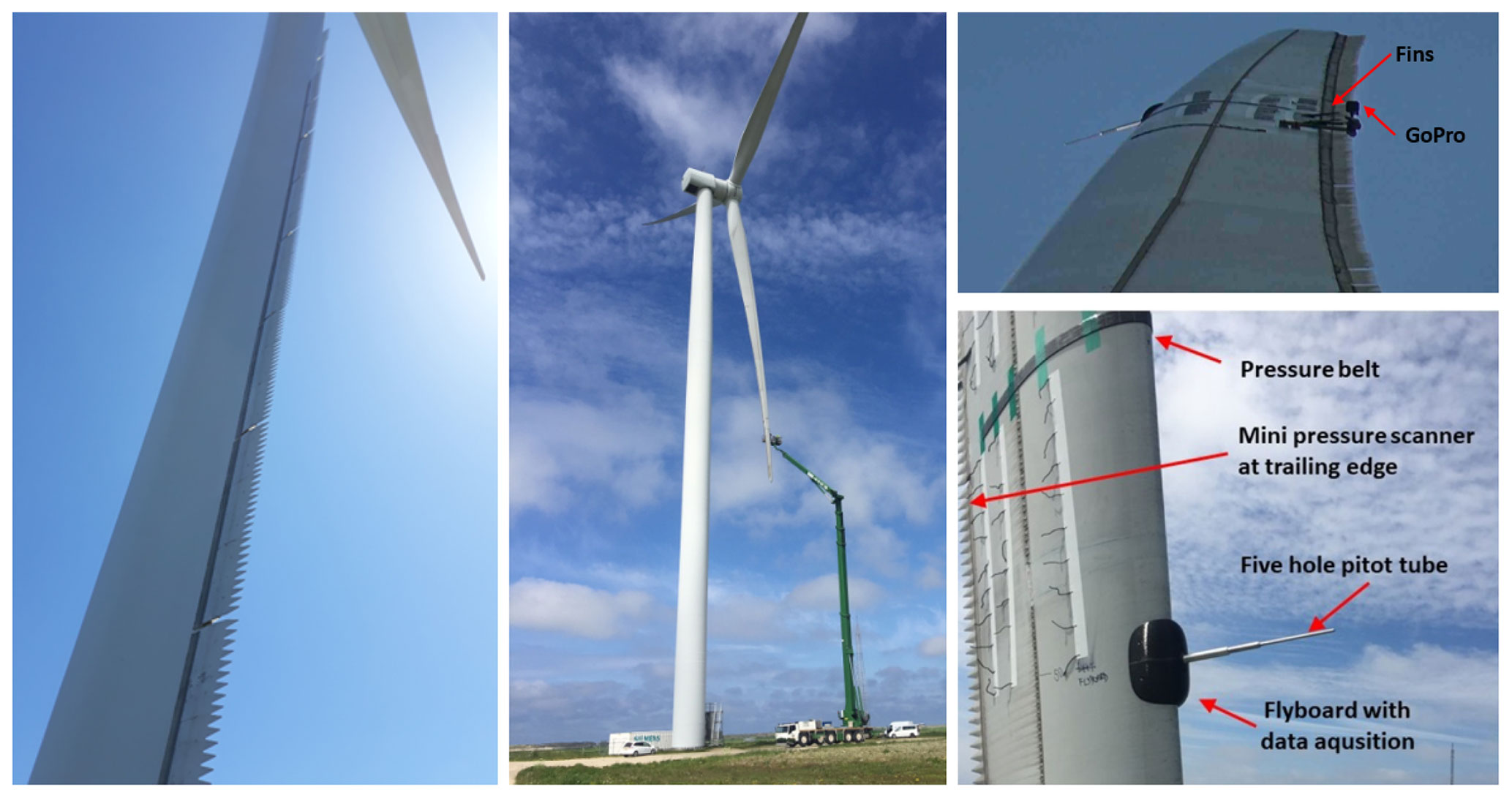
Figure 1 Left photo: active flap placed on the trailing edge of the blade of the Prototype at the Høvsøre test field. Central photo: installation of the flyboard and pressure belt in June 2020. Bottom right photo: close look at the flyboard and the pressure belt. Top right photo: camera and fins installed to measure the flap deflection. Photos courtesy of SGRE and DTU.

In June 2020, an inflow and pressure measurement system was temporarily added to the Prototype to measure the aerodynamic properties at a specific ATEF section, as described in Madsen et al. (2022) and shown in the central photo of Fig. 1. The system, developed by DTU, consisted of an inflow five-hole pitot tube sensor, a belt with 15 pressure taps, and an autonomous data acquisition and transmission system (flyboard). Both pitot tube and flyboard were installed on the blade leading edge at 50 m from the hub flange, in the middle of the spanwise extension of the flap. The pressure belt was wrapped around the blade at a spanwise position of 49 m. The inflow and pressure measurement system provided data with a 100 Hz sampling rate that was synchronized with the Prototype measurement data by the recorded GPS time. A close view of the pressure belt and flyboard is shown in the bottom right photo of Fig. 1.

Additionally, two couples of small plastic fins were installed near the pressure belt location to analyze the ATEF deflection visually. The fins of each couple lay aligned on the same blade section, with the two couples spaced around 0.5 m apart spanwise. For each couple, one fin was attached to the moving ATEF and the other to the blade structure. A GoPro camera was installed close by to record the flap deflection using the fins as reference points, as shown in the top right picture of Fig. 1.

3 Aeroelastic setup

3.1 BHawC model

SGRE has internally developed and validated the aeroelastic engineering tool BHawC, based on the blade element momentum (BEM). Furthermore, SGRE has developed an ATEF module to model the flap aerodynamic and actuator system. The model uses the instantaneous value of the flap angle (or flap state) to interpolate the instantaneous steady 2D aerodynamic characteristics of the flap sections from a pre-generated set of 2D steady aerodynamic properties provided for a range of flap angles (or flap states). These properties are then provided to the global wind turbine model to replace the 2D aerodynamic blade characteristics in the blade sections equipped with flaps.

The BHawC model adopted in this paper was provided by SGRE and fine-tuned by the authors in Gamberini et al. (2022), where the aeroelastic model was able to estimate the Prototype operational parameters with a maximum error lower than ±3 % and blade loads within ±2 % for the flap in stationary state. The current paper covers the tuning and validation of the ATEF actuator and aerodynamic model during the dynamic actuation of the flap.

3.2 HAWC2 model

HAWC2 is the BEM aeroelastic engineering tool developed by DTU Wind. It models the active flap with ATEFlap, an advanced “engineering” model that not only computes the 2D steady aerodynamic properties of a flap section but also directly computes the unsteady aerodynamic forces and pitching moments due to arbitrary deflection and motion of the flap. Under the assumption of plane wake separation, trailing edge stall separation, and uniform upwash velocity along the chord, ATEFlap can describe the dynamic of the forces related to the flow separation and the effects of the vorticity shed into the wake (Bergami and Gaunaa, 2012).

The authors tuned the HAWC2 model of the SGRE Prototype in Gamberini et al. (2022), based on the BHawC model, obtaining negligible code-to-code differences (maximum difference below 1 %) for mass properties and wind turbine operational parameters and a maximum difference within 4 % for the blade loads. For the ATEFlap model, the suggested values of the coefficients for the indicial response exponential function and the exponential potential flow step response were used. These parameters were tuned to describe the step response of the NACA 64-418 airfoil (18 % thickness), which can be considered an acceptable approximation for the modeled flap.

3.3 Modeling of the flap system

The ATEF system installed on the Prototype is simplified as a controlled pneumatic system regulating the pressure inside the hose connected to the active flap. Increasing the air pressure inflates the hose that deflects the flap. The flap deflection changes the blade section shape, consequently modifying the local aerodynamic forces and affecting the loading of the whole Prototype.

In the ATEF aeroelastic model, depicted in Fig. 3, the pneumatic system and the flap structure are merged in the actuator model. This model directly links the controller signal of the flap state to the flap deflection, disregarding the air pressure signal. This simplification is possible because the controller system controlled only the final pressure value and the pressure valve actuation time. The variation in the air pressure inside the hose after the valve actuation depended only on the layout of the pneumatic and flap systems after the valve (for example the length, diameter, and material of the hose and the stiffness of the flap). Therefore, the air pressure and the corresponding flap deflection were expected to have a similar transient response for each pressure valve actuation.

The actuator model provides the flap deflection to the aerodynamic model that computes the dynamic aerodynamic properties of the flap section, which is needed by the aeroelastic code to calculate the Prototype loads. In both codes, the ATEF aerodynamic model relies on the flap airfoils' stationary lift and drag coefficient (Cl and Cd) data for active and deactivated flap states. The flap was installed over a longitudinal blade section with thickness ranging from 24 % to 18 % of the chord; therefore, the aerodynamic characteristics of the flap airfoils with thickness between 24 % and 18 % are needed. SGRE provided the aerodynamic characteristics of the 21 % thickness airfoil of the blade equipped with the flap. Similar to the method described in Gomez Gonzalez et al. (2018), SGRE measured the aerodynamic characteristics in a wind tunnel campaign performed at the low-speed, low-turbulence wind tunnel facilities of the faculty of aerospace of TU Delft. The measurements, most of them run at a Reynolds number of 4 million, focused on the 21 % thickness airfoil where three different shapes of the deflected flap were modeled with a corresponding fixed add-on. The measurements provided the aerodynamic characteristics for the flap that was not active and active at low and high actuation pressures. The data for middle actuation pressure are obtained by interpolation, as previous tests in the VIAs project showed a linear relation between flap deflection and pressure for the studied ATEF system. The aerodynamic characteristics of the 24 % and 18 % thickness airfoils are computed assuming that the same flap deflection leads to the same lift and drag variation across the family of flap airfoils. Under this assumption, from the 21 % thickness airfoil, the lift and drag increases due to a specific flap deflection are calculated as a function of the angle of attack. These ΔCl and ΔCd are added to the 24 % and 18 % thickness airfoil properties after being linearly scaled to adjust to the actual chord length of the new airfoils. Figure 2 shows an example of curves of the normalized Cl versus angle of attack for flap not active (black line) and active at low pressure (red line) of the 21 % (left), 18 % (top right), and 24 % (bottom right) thickness airfoils. It also shows the ΔCl obtained from the 21 % thickness airfoil (center). The ATEFlap model of HAWC2 requires the aerodynamic properties to be in a specific format, where aerodynamic coefficients are given as a function of the angle of attack and the angle of flap deflection. This format is obtained utilizing the Preproc ATEFlap tool. The BHawC flap model directly provides the instantaneous stationary 2D aerodynamic properties to the global wind turbine model. Instead, the HAWC2 ATEFlap model computes already the unsteady effects due to flow separation and the vorticity shed into the wake, providing the instantaneous dynamic aerodynamic properties to the global wind turbine model.

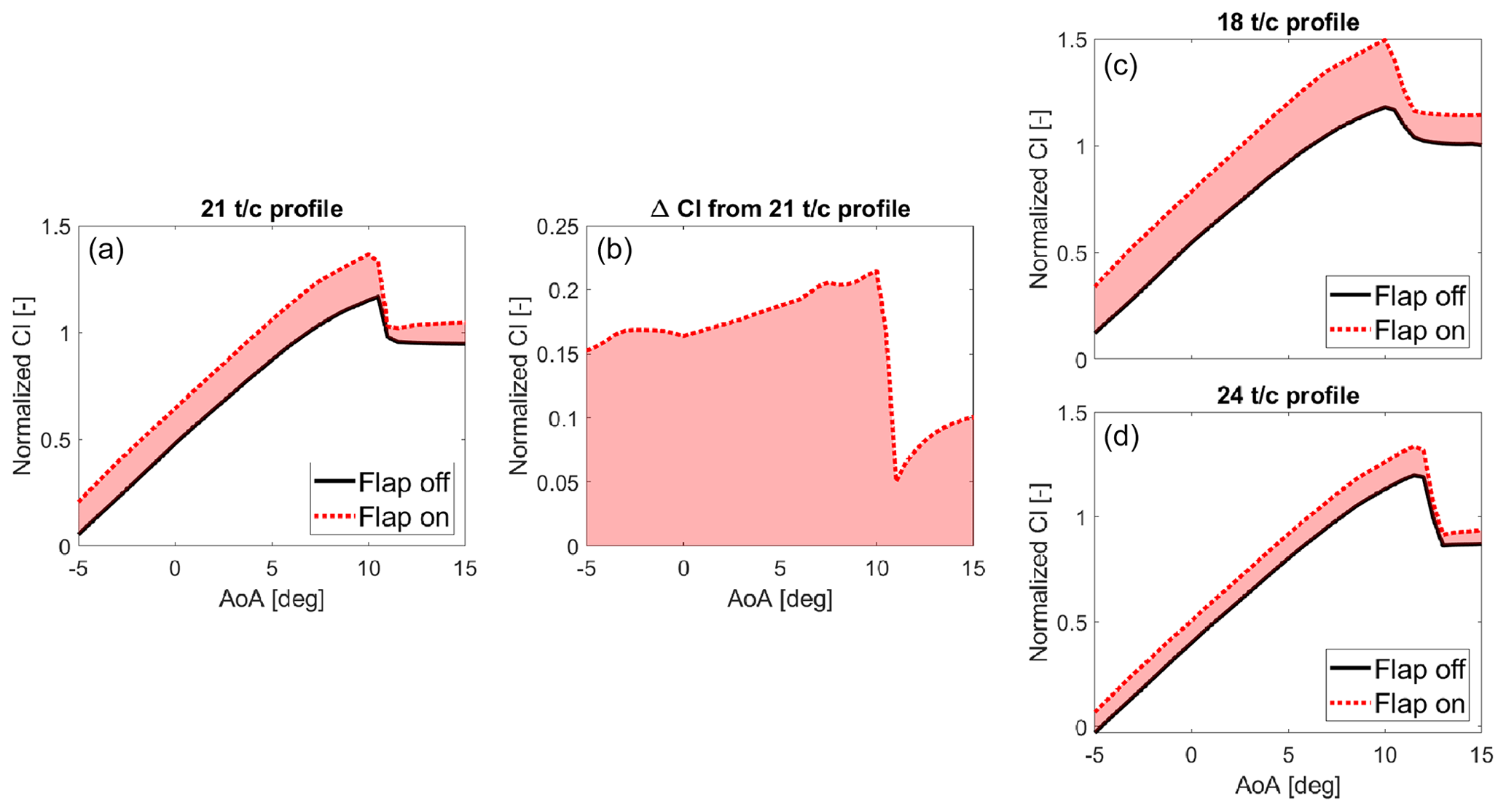
Figure 2 (a) Normalized Cl versus angle of attack (AoA) of the 21 % thickness airfoil with flap not active (black) and active at low pressure (red dotted line). (b) ΔCl from the 21 % thickness airfoil due to flap activation. Normalized Cl versus angle of attack of 18 % (c) and 24 % (d) thickness airfoils with flap active at low pressure (red dotted line) obtained by adding the scaled ΔCl from the 21 % thickness airfoil to the curves with flap not active (black lines).

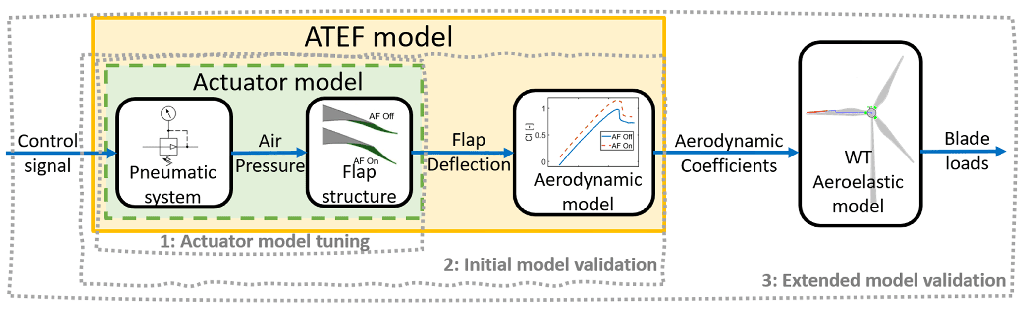
Figure 3 Structure of the ATEF aeroelastic model implemented in BHawC and HAWC2. Dotted-edged rectangles indicate the model elements involved in the three validation steps.

4 Actuator model tuning

To validate the aerodynamic model, a reliable flap actuator model is needed to compute the position and motion of the flap. In this paper, the tuning of the flap actuator model is obtained by the analyses of video recordings of the Prototype flap actuation.

In June 2020, a GoPro camera and two sets of plastic fin were temporarily installed on the Prototype blade. The camera captured the movements of the flap during its activation and deactivation under three distinct actuation pressure levels (low, middle, and high) and two operational states of the wind turbine: idling mode and normal operation at 6 rpm. Each combination was repeated four times to ensure data reliability. The video analysis and modeling tool Tracker (Brown et al., 2023) is utilized to extract the flap deflection in each video by tracking the relative position of the two fins during the flap activation and deactivation. For each combination, the four recorded cases consistently yield a similar flap deflection response during flap activation; their binning and normalization result in the characteristic flap activation deflection response (activation deflection curve) that ranged between 0 (flap not active) and 1 (flap fully deployed). The characteristic flap deflection response for deactivation (deactivation deflection curve) is obtained with a similar process.

The comparison of the flap deflection responses shows a substantial overlap of the curves obtained for middle and high actuation pressure, with the low-pressure case being slightly faster. Although increasing the actuation pressure results in higher flap deflection, the normalized flap deflection curve is independent of the activation pressure for middle- and above-pressure values. Furthermore, the flap displays a slower activation and a faster deactivation when the wind turbine is in normal operation compared to the idling state. The latter behavior can be attributed to the effect of the aerodynamic pressure distribution on the blade section, which generates an aerodynamic force opposing the flap deflection during activation and supporting it during deactivation. The magnitude of this aerodynamic force, higher in the normal operation state compared to the idling state, directly affects the time required for full activation and deactivation, with higher forces resulting in slower activation and quicker deactivation.

In modeling the flap actuator, it is assumed that the activation and deactivation curves are independent of the target actuation pressure. This assumption is valid for high- and middle-actuation-pressure scenarios covering most of the available Prototype field data. The actuator model should also include the impact of the aerodynamic loads on the flap dynamic, which varies in the function of the wind speed and wind turbine operational state. Therefore, the middle- and high-pressure deflection curves for normal production were selected, assuming a negligible change in the impact of the aerodynamic load around the measured operative condition. The neglection of the impact of the aerodynamic loads on the total flap deflection is also based on the results from Gamberini et al. (2022), where the stationary flap properties were validated for a wide range of wind speeds.

On the Prototype pneumatic system, the signal of the flap state controller was not recorded. Therefore, the pressure channel is initially used to identify the flap controller activation time, assuming no delay between the controller activation and the opening of the pressure valve. The flap actuator is finally modeled as a simple second-order transfer function without poles. A fourth-order polynomial function was added to improve the similarity to the deflection curve data. In Fig. 4a, the activation deflection curve for middle and high actuation pressure (black line) with the error band of 1 standard deviation (SD) is compared with the modeled second-order transfer function (blue dotted line) and the improved model with the fourth-order polynomial function (red dashed line with circles). Similarly, Fig. 4b compares the experimental and modeled flap deactivation curves.

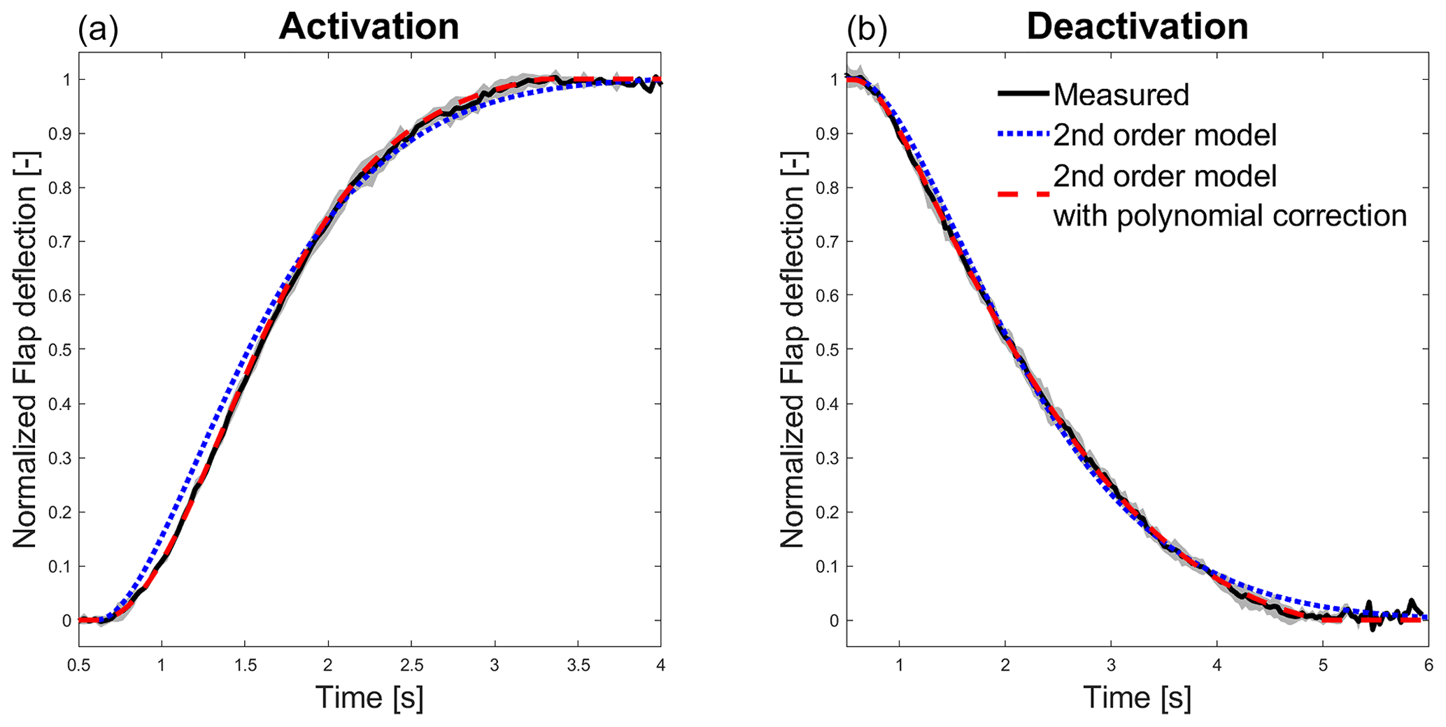
Figure 4 Normalized flap deflection curves measured with the video tracking (black line), obtained from the second-order transfer function model (blue dotted line) and from the second-order transfer function model fine-tuned with a fourth-order polynomial function (red dashed line with circles) for flap activation (a) and deactivation (b). The measured lines are shown with the mean value line enveloped by the gray 1 SD error band.

5 Initial ATEF aerodynamic model validation

The aerodynamic model of the ATEF aeroelastic module is initially validated for a single Prototype blade section equipped with the active flap. This validation relies on a 3 h measurement dataset with an almost constant wind speed. It compares the transient response of the lift coefficient measured on the Prototype blade section with the Cl transient response curve calculated via aeroelastic simulations during the flap activation and deactivation. In addition, the validation includes comparing the measured and simulated transient responses of the blade-to-blade flapwise bending moment at the root of the blades.

5.1 Measurements

In June 2020, an inflow and pressure measurement system was temporarily mounted on the Prototype in the middle of the blade span equipped with the active flap for around 1 d (Madsen et al., 2022). The measurement system comprised a pressure belt with 15 taps, a “flyboard” with the data acquisition system, and a five-hole pitot tube measuring the local inflow to the blade section. The data acquisition system in the flyboard sampled the data from the pressure scanners and the five-hole pitot tube with a sampling rate of 100 Hz. The captured raw data from the flyboard and pressure belt were processed and converted into quantities of interest. This process included calibrating the pitot tube pressure data and conversion into two flow angles (inflow and sideslip angles) and a velocity. The inflow measurement quantities were further corrected to transform the pitot tube inflow angle into the airfoil angle of attack and relative velocity. This transformation was based on 2D CFD simulations performed by SGRE on the airfoil section for zero and full flap states, where the flow velocity and angle at the point of measurement of the pitot tube were extracted as a function of the geometric angle of attack (see Madsen et al., 2022). The pressure belt data were integrated into 2D aerodynamic forces by chordwise trapezoidal integration of the pressures, where a trailing edge pressure was added as an average of the two nearest points. The local pressure and lift coefficients (Cl) were calculated using the corrected dynamic pressure and angle of attack from the pitot tube. Due to uncertainties in the conversion process based on 2D CFD, the absolute value of the angle of attack and the consequent absolute Cl cannot be used for the validation. Therefore, the lift coefficient validation focuses on comparing the normalized Cl transient responses that are unaffected by the conversion uncertainties.

During most of the measurement period, the wind speed was relatively low, between 4 and 6 m s⁻¹, keeping the wind turbine close to the minimum operational rotor speed. For the validation, a 3 h time interval characterized by a relatively constant wind (10 min mean wind speed between 4 and 5 m s⁻¹) with low turbulence intensity (below 10 %) is selected from the measurement period. The low variation in mean wind speed and low turbulence intensity is beneficial in reducing the variability range of the lift coefficient, facilitating the calculation of the average Cl transient curve during flap actuation. In the selected time interval, the flap was performing on–off actuation cycles, switching between 60 s at middle-pressure actuation and 60 s at deactivated state, completing a total of 90 cycles.

5.2 Aeroelastic simulations

The aerodynamic setup of the BHawC and HAWC2 models is configured as similarly as possible to minimize the differences between the aeroelastic models. Both models have the BEM implemented on a polar grid, as described in Aagaard Madsen et al. (2020), to better account for the rotor induction imbalance due to the flap equipped on only one blade. Furthermore, they implement a potential flow tower shadow model linked to the tower top movements.

The same set of aeroelastic simulations is performed with the two aeroelastic codes to compute the average Cl transient curve during flap activation and deactivation. The set consists of 12 simulations with flap actuation happening at evenly spaced azimuth angles. All simulations are 2 min long, with a constant wind speed of 5 m s⁻¹ without turbulence, with standard air pressure and a wind shear of 0.2. The flap starts in the deactivated position, is activated at t=30 s, and is deactivated after 60 s, at t=90 s, reproducing the activation and deactivation cycles performed on the Prototype. The flap actuator models of both BHawC and HAWC2 Prototype aeroelastic models are updated to match the tuning described in Sect. 4. The Cl is calculated at the blade section where the pressure measurement system was installed.

5.3 Average lift coefficient transient response curve on a wind turbine blade section

The rotor cone and tilt angles of the wind turbine, together with the variations in wind speed resulting from wind shear, veer, and large turbulence structures, contribute to periodic fluctuations in the lift coefficient. These fluctuations challenge the detection and characterization of the CL transient response caused by flap actuation. The averaging of cases with flap actuation occurring at different azimuthal positions substantially reduces the azimuth-dependent variation in Cl, with the quality of the average Cl transient curve improving as the flap actuation azimuthal positions are more evenly spread and balanced. Ideally, the curve should be obtained by averaging an equal number of actuation responses starting at every azimuthal angle.

In the case of the aeroelastic simulations, the average Cl transient curve is derived through the binning (based on the simulation time) of the 12 simulations, each with the flap actuation happening at an evenly spaced azimuth angle. Figure 5a shows the Cl time series (dotted lines), normalized to the average Cl increase, from the BHawC simulations around the flap activation time (t=0 s). The azimuth-dependent oscillations of Cl amount to around 40 % of the Cl variation due to flap activation (ΔCl_F) and affect the slope and shape of the Cl transient curve during the flap activation. Instead, the average of the Cl curves (black line) is constant before the activation; then, it rises at an almost constant rate until it settles to a constant value after approximately 2.5 s. A similar pattern, but with a longer settling time of around 5 s, is exhibited during flap deactivation, as shown in Fig. 5b. The results from the HAWC2 simulations are almost identical to the BHawC results and are not included in this chapter for brevity.

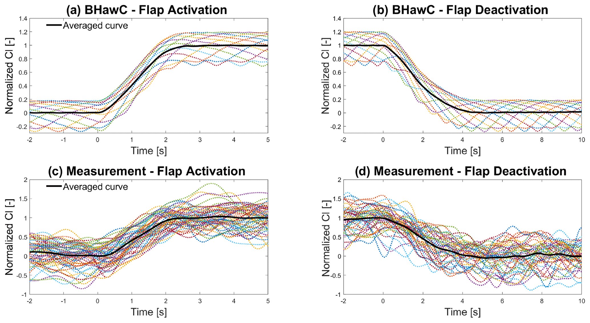
Figure 5 Panels (a) and (b) show the normalized averaged Cl transient curve (black line) for flap activation and deactivation obtained from averaging the Cl signal of 12 BHawC simulations (dotted lines). Similarly, panels (c) and (d) show the normalized averaged Cl transient curve (black line) for flap activation and deactivation obtained from averaging the measured Cl signals (dotted lines).

Regarding the measurement data, the times of flap actuation (both activation and deactivation) are determined by identifying the instant at which the gradient of the flap actuation pressure started to change. Subsequently, the Cl time series are segmented into temporal windows centered around the flap actuation time and synchronized accordingly. The average Cl transient curve is finally obtained by binning the Cl signals based on the time window. Different filtering techniques have been tested to reduce the oscillation of the averaged curve caused by turbulence and measurement noise. The best results are achieved with a low-pass, zero-phase digital filter set to attenuate frequencies above 9 P (9 times the rotor rotational frequency) without affecting the slope of the Cl transient. For accurate validation, synchronizing the Cl measurements with the Prototype measurements is crucial in ensuring the precise timing of the Cl variation relative to flap actuation pressure. The synchronization relies on the GPS time recorded by the flyboard, further refined by aligning the time of maximum acceleration along the blade length (also measured on the flyboard) with the time the blade is oriented toward the ground. In the average Cl curve calculation, some measurements are discarded due to insufficient data quality, reducing the transient cases to 46 for activation and 63 for deactivation. The measurements have an acceptable distribution of the azimuthal angle at flap actuation, as shown in Table 1, with three cases or more for all sectors. Figure 5c shows the normalized measured Cl curve during flap activation (dotted lines). These curves exhibit a higher variability than the aeroelastic simulation curves, with a range of the same order of amplitude as the increase in Cl due to flap activation. The wind turbulence is another cause of the measurement's variability, a parameter omitted in the simulations due to the difficulties in estimating the correct turbulence value for a very short simulation time. Nevertheless, the averaged Cl transient curve (black line) exhibits a clear and almost linear variation from a slightly decreasing value before the activation to an almost constant value after the activation. The averaged Cl transient during flap deactivation (black line in Fig. 5d) shows a higher fluctuation behavior than the activation transient but is still considerably smoother than the measurements.

Table 1 Number and azimuth distribution of measured cases used to calculate the average Cl transient and average blade-to-blade moment difference (BMD) during flap activation and deactivation.

5.4 Blade-to-blade azimuth-based blade root moment

Another crucial aspect for validating the aeroelastic model of the ATEF is the analysis of the blade root bending moment transient response resulting from flap actuation. However, measuring this load transient proved challenging due to its high-frequency response, often hidden within the complex dynamics of the blades responding to factors such as turbulence, shear, vibrations, and rotation. Gomez Gonzalez et al. (2021) introduced a blade-to-blade (b2b) analysis method to compute the load transient response caused by the ATEF actuation. This approach involves calculating the difference between the loads acting on the blade with the flap and the load acting on another blade without the flap but delayed by a time corresponding to a third of one rotor rotation. This artificial time shift aims to synchronize the load time series of blades in the same azimuthal position, thereby mitigating the influence of periodic signal dynamics resulting from rotation, forced vibrations, and wind shear.

This paper proposes a novel azimuth-based b2b method (az-b2b) calculating the load difference by interpolating the loads based on the cumulative azimuth position instead of relying on time shifting. The method comprises three steps. Firstly, the cumulative sum of the azimuthal angle is calculated for each blade. Secondly, the load of the blades without the flap is interpolated as a function of the cumulative sum of the azimuthal angle of the blade with the flap. Lastly, the difference between the load of the blade with the flap and the interpolated load of the blade without the flap is calculated.

Notably, the az-b2b method eliminates the need to initially segment the time series around the relevant event, as the previous b2b method required, and it can be applied directly to the entire time series in a single run. Additionally, the az-b2b method is not dependent on the calculated mean rotor speed, which is influenced by the time extension of the segments. This characteristic makes it less sensitive to minor variations in rotor speed. By ensuring that the load difference is calculated between two blades positioned at the same azimuthal location, the az-b2b method effectively reduces azimuthal-dependent load fluctuations. However, the precise measurement of the azimuthal angle is essential to avoid errors during the interpolation phase. Like the original b2b method, the az-b2b method is still sensitive to high rotor speed variation that can result in a significant variation in data density for azimuthal angle, potentially affecting the quality of the interpolation result.

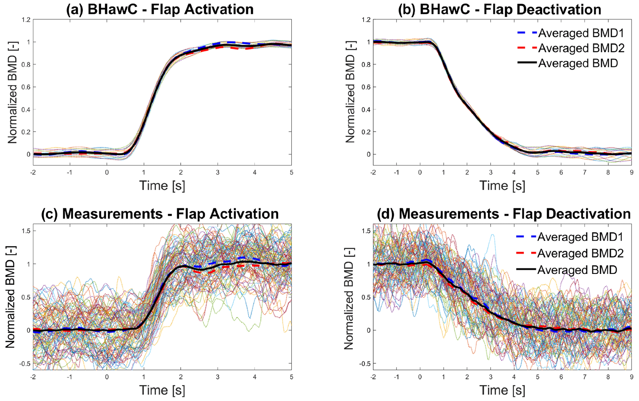
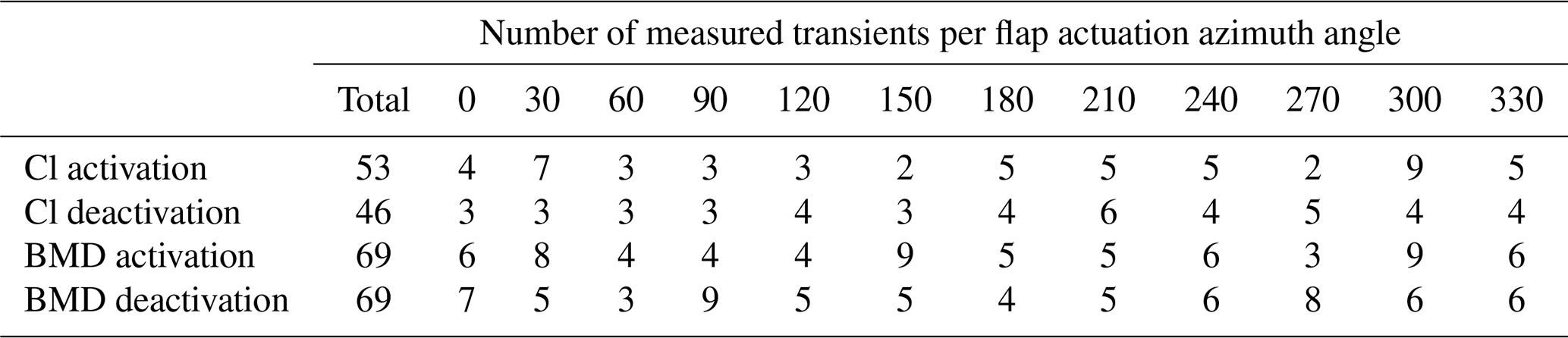
Figure 6 Panels (a) and (b) show the normalized averaged b2b bending moment difference at blade root (BMD) transient curve (black line) for flap activation and flap deactivation, obtained from the averaging of the BMD signals of 12 BHawC simulations (dotted lines). Similarly, panels (c) and (d) show the averaged normalized BMD transient curve (black line) for flap activation and deactivation, obtained from averaging the measured BMD signals (dotted lines). All the plots also include the b2b bending moment difference between the blade with the flap and blade 1 (BMD1: blue dashed line) and blade 2 (BMD2: red dashed line).

The az-b2b method is utilized to calculate the differences in flapwise bending moments at the blade root between the blade with the flap and the remaining blades (blade 1 and blade 2) in the aeroelastic simulation sets of BHawC and HAWC2. As shown later in this paper, the two blade-to-blade differences do not differ significantly in both simulations and measurements; therefore, the mean of the two azimuth-based blade-to-blade flapwise bending moment differences at the blade roots (BMD in the remaining part of the paper) is used as a reference channel. Finally, the binning (as a function of the simulation time) of the 12 simulation signals computes the average BMD transient curve. Figure 6a shows the normalized BMD curves (dotted lines) obtained from the BHawC simulations, together with the normalized average BMD transient curve (black line). All the signals are normalized in order to make the increase in the b2b moment due to flap actuation unitary. The azimuthal variability in the BMD curves is present but significantly lower than the Cl curves, being less than 10 % of the average transient curve. The average BMD curve is almost constant before the flap actuation, and then it rises smoothly from around 0.5 s until it converges to an almost constant value after 2 s. The average curves of the individual b2b differences (blue dotted line and red dotted line) exhibit only a slight difference between themselves. Similar considerations are valid for the BMD curves during flap deactivation shown in Fig. 6b. The BMD curves from the HAWC2 simulations were almost identical to the BHawC results and are not included in this chapter for brevity.

Regarding the measurement data, the same methodology employed for the Cl transient is applied to compute the blade load difference. The measurement signals are segmented into temporal windows centered around the actuation time and synchronized accordingly. Subsequently, the consistency of the azimuthal angle signal is verified, and the rotor speed is leveraged to compute the missing or erroneous values. Afterward, the BMD curves are computed, and the average BMD transient curve is obtained using the binning approach. The average BMD calculation uses the same number of measured time series (69) for flap activation and deactivation. The distribution among the rotor sector of the flap actuation azimuthal angle is also acceptable, with most sectors having at least five cases. Similar to the results from the Cl transient curves, the BMD-measured transient curves (dotted lines in Fig. 6c) show a high oscillation, partly caused by the wind turbulence, with a range comparable with the load increase due to the flap activation. Nevertheless, the averaged BMD transient curve (black line) is almost constant before the activation and then smoothly increases and converges to the flap actuation value with minor oscillations. The average curves of the individual b2b differences are also close to each other, with a maximum difference of 0.1 normalized BMD. Similar considerations can be given for the flap deactivation case, shown in Fig. 6d.

5.5 Initial validation results and discussion

To compare the simulation results with the measurements, the actuation pressure signal is used to synchronize the transient curves. In detail, the time the flap pressure gradient undergoes a quick change is aligned with the flap activation time in the simulations. For the deactivation case, an additional delay of 0.3 s is added to the simulation flap deactivation time to properly align the simulated Cl and blade-to-blade loads with the measurements. The authors believe this delay is related to the structure of the pneumatic actuator system, and it would have been identified during the actuator system tuning if the flap state controller signal had been available. For the activation phase, a time delay is not clearly needed.

Figure 7 Comparison of the normalized averaged Cl transient curves obtained from BHawC (blue dashed line with x marker) and HAWC2 (red dash-dotted line) simulations and measurements (black line with asterisk marker) during flap activation (a) and deactivation (b), including an error band of 1 SD of the matching colors. The normalized measured flap pressure (blue dotted line) and the estimated flap control signal (black dashed line) are also included.

Figure 7a compares the simulated and measured Cl transient curves for flap activation and Fig. 7b for flap deactivation. In the figures, the synchronized flap actuation time is indicated by the estimated flap control signal (black dashed line), used in the simulation to actuate the flap, and the measured flap pressure signal (blue dotted line). The average Cl curves from BHawC (blue dashed line with x marker) and HAWC2 (red dash-dotted line) simulations closely match each other, with a maximum difference below 6 % of the ΔCl generated by the flap actuation in both flap activation and deactivation cases, mainly caused by an offset of two time steps (0.04 s) between the two transients. The simulated average Cl curves are significantly similar to the measurements (black line with round markers). In the activation case, the maximum difference is below 40 % of the measurement SD, below 8 % of the ΔCl, with the simulated Cl curves starting to increase 0.1 s (5 % of the time for full flap activation) before the measurement curves but at a lower slope, and they converge to full activation with a delay of 0.15 s (7.5 % of the complete flap activation time). In deactivation, the maximum difference is below 6 % of the measurement SD, below 8 % of the ΔCl. The simulated Cl curves start to decrease with a delay of 0.2 s (4 % of the full flap deactivation time) that quickly recovers. Afterward, they precede the measurement curve by less than 0.1 s (2 % of the full flap deactivation time) until full deactivation. The SDs of the simulated curves are often equivalent. They are nearly half of the measurement SD, mainly due to the omission of turbulence in the aeroelastic simulations.

The b2b moment transient curves are compared in Fig. 8a for flap activation and Fig. 8b for flap deactivation. Similar to the Cl comparison, the average BMD transient curves from BHawC (blue dashed line with x marker) and HAWC2 (red dash-dotted line) simulations closely match each other, with a maximum difference below 7 % of the ΔBMD due to the flap actuation in both flap activation and deactivation cases, mainly caused by an offset of 0.06 s between the two curves. Both curves have an SD significantly smaller compared to the Cl curves, showing the benefit of the az-b2b method in removing the impact of the azimuthal load oscillations. The HAWC2 curve shows an SD almost twice that of the BHawC simulations. The main reason is a higher oscillation in the rotor speed originating from an imperfect implementation of the SGRE controller in the HAWC2 code. The simulated average BMD curves are similar to the measurements (black line with round markers). In the activation case, the maximum difference is below 55 % of the measured SD and 17 % of the ΔBMD due to the flap activation. Mirroring the Cl transient curves, the simulated BMD begins to increase 0.2 s (10 % of the complete flap activation time) before the measured BMD but at a lower slope, and it converges to full activation within the measurement fluctuation transient. In the deactivation, the maximum difference is below 60 % of the measured SD, below 20 % of the ΔBMD. The simulated Cl curves start to decrease with a delay of 0.2 s (5 % of the complete flap deactivation time) that is quickly recovered. Afterward, they precede the measurement slope by less than 0.1 s until complete deactivation.

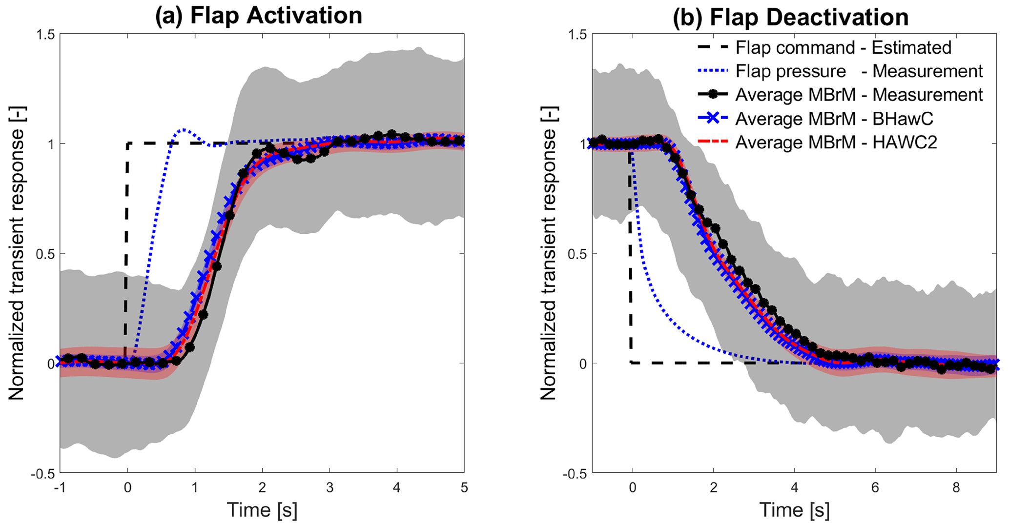
Figure 8 Comparison of the normalized averaged b2b blade root bending moment (BMD) transient curves obtained from BHawC (blue dashed line with x marker) and HAWC2 (red dash-dotted line) simulations and measurements (black line with asterisk marker) during flap activation (a) and deactivation (b), including an error band of 1 SD of the matching colors. The normalized measured flap pressure (blue dotted line) and the estimated flap control signal (black dashed line) are also included.

Another purpose of the initial validation is tuning the ATEF model to ensure the proper synchronization between the simulated and measured Cl and BMD transient curves. Figure 9a shows all the signals relevant for the ATEF aeroelastic model tuning during flap activation. The flap state controller signal was not recorded in the measurement campaign. Therefore, the measured flap pressure (blue dotted line) synchronizes the simulated flap control signal (black dotted line). This control signal commands the flap deflection (red dashed line with circular markers), the deflection obtained from the postprocessing of the flap deflection videos (green squared markers). The Cl transient follows the flap deflection by a few milliseconds in the simulations (blue line with squares and orange line) and by 0.1 s in the measurements (gray line with arrow marker). The slight difference between the simulated and measured Cl transients (especially if compared to the measurement SD) confirms the current model (with a linear relation between flap deflection and Cl variation) provides reliable results. The simulated BMD curve rises 0.5 s after the Cl increase, anticipating the measured curve by 0.2 s. Figure 9b shows the signals relevant for the ATEF model tuning during flap deactivation. To properly align the simulated Cl and BMD curves with the measurements, a delay of 0.3 s is introduced in the actuator model between the flap state controller and the flap deflection during deactivation only.

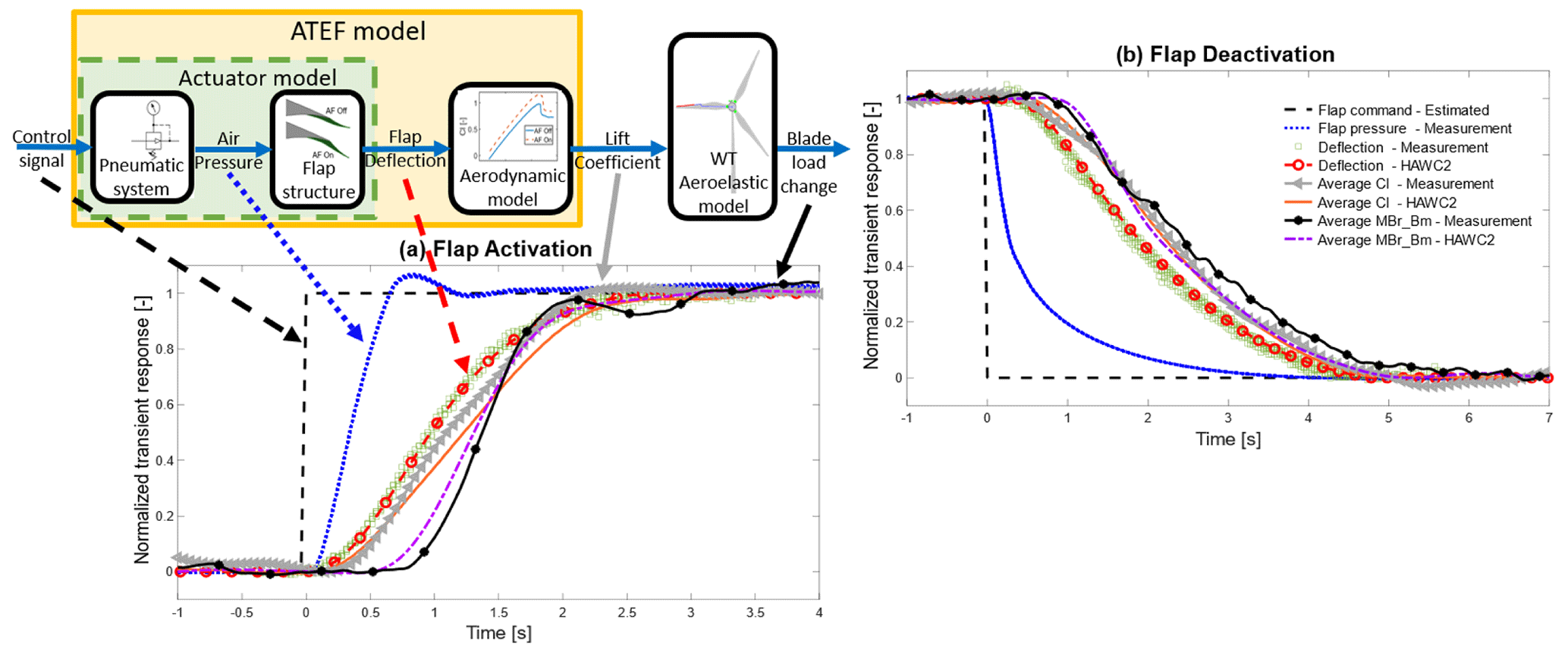
Figure 9 (a) Signals relevant for modeling and validating the flap model during flap activation linked to the ATEF model scheme. Estimated flap state controller (black dashed line), normalized flap pressure (blue dotted line), measured and simulated flap deflection (green squares and red dashed line with circles), measured and simulated Cl curves (gray line with triangle and red line), and measured and simulated BMD curves (black line with asterisks and violet dash-dotted line) are plotted to verify the time tuning of the aeroelastic model. (b) Signals relevant for the modeling and validation of the flap model during flap deactivation.

In conclusion, the initial validation showed a good agreement between the simulated and measured average Cl and BMD transient curves. However, small differences in the curves motivate the broader validation described in the following section.

6 Extended ATEF aerodynamic model validation

The validation of the ATEF aerodynamic models is extended to a wider range of environmental conditions with the measurements obtained from the Prototype field campaign run between October and December 2020. In this part of the test campaign, the flyboard was not present, and the validation can rely only upon comparing the transient of the blade-to-blade moment at the blade root during flap activation and deactivation. The validation follows the so-called one-to-one approach, where the measurements are compared with a set of simulations reproducing the wind turbine operating under the same environmental conditions measured at the time of the flap actuation. As the validation focuses on the short transient happening within 10 s after the flap activation and deactivation, the simulations rely not on the 10 min averaged environmental condition but on the actual condition measured at the flap actuation time.

6.1 Field campaign

Between October and December 2020, the ATEF system on the Prototype was tested for several actuation pressure and activation patterns. The measurements of full activation and deactivation cycles at middle actuation pressure with the Prototype operating in normal production are selected for validation. Additional filtering removes the measurements at which the wake of the Prototype or the nearby wind turbines affected the met mast measurements. As a change in the wind turbine operative condition could result in a BMD variation and interfere with the load transient response due to flap actuation, only flap actuation occurring when the Prototype was in almost stationary condition is selected. This selection is achieved by removing the cases where, within 10 s before and after the flap actuation, the pitch angle varied by more than 1°, the rotor speed more than 0.5 rpm, and the yaw direction more than 1°. Finally, a total of 150 measurements for flap activation and 135 for flap deactivation are obtained, distributed between 5 and 20 m s⁻¹, as shown in Fig. 10a.

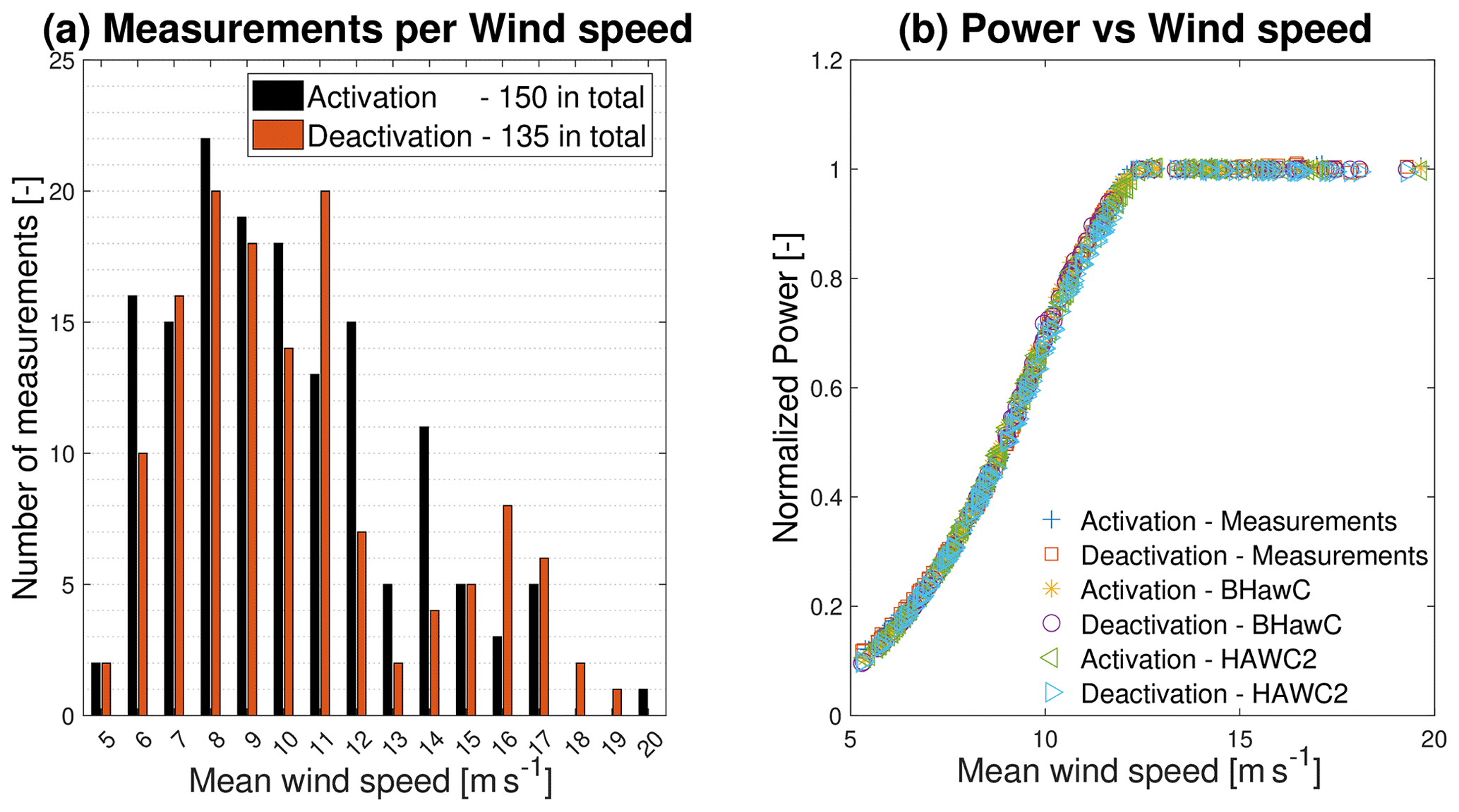
Figure 10 (a) Number of selected measurements per wind speed for flap activation (black) and deactivation (red). (b) Normalized power curve of the selected measurements and simulations (BHawC and HAWC2) for flap activation and deactivation.

6.2 Model and simulation setup

The BHawC and HAWC2 models from the initial validation described in Sect. 5 are used for this validation, including the additional 0.3 s deactivation delay in the flap actuator model.

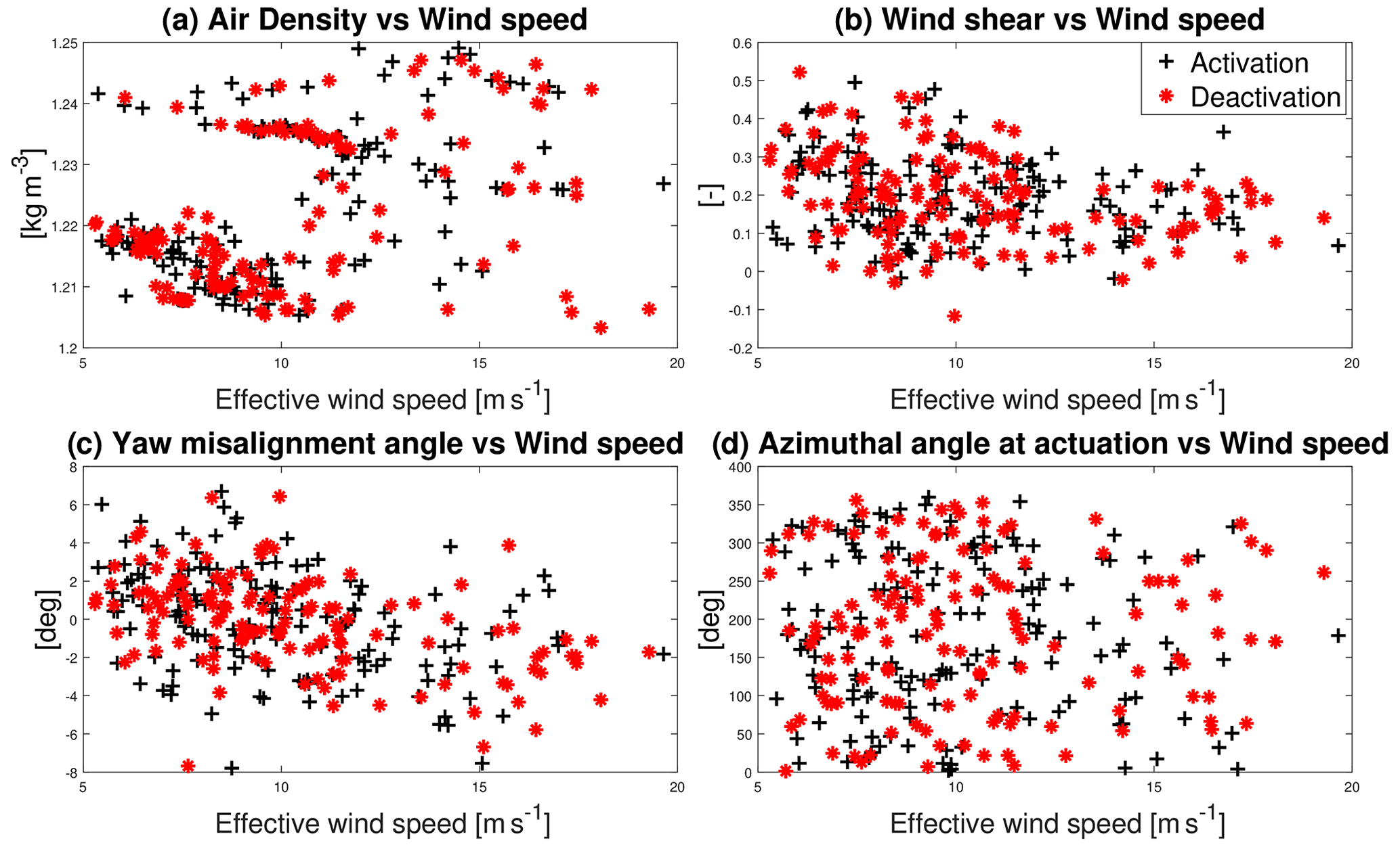
Figure 11 Distribution of air density (a), wind shear (b), yaw misalignment angle (c), and azimuthal angle at flap actuation (d) in function of the effective wind speed used for the flap activation (black cross) and deactivation (red asterisk marker) aeroelastic simulations.

To properly calculate the b2b load transient curve during flap actuation, the simulation setup has to match the environmental conditions at the wind turbine at the specific time of the flap actuation. The environmental conditions were measured at the met mast, located 300 m in front of the Prototype. This distance introduced a time delay T_d corresponding to the time the wind needs to cover the distance D_m between the met mast, where it was measured, and the wind turbine rotor. This delay is inversely proportional to the wind speed (T_d=60 s for a low 5 m s⁻¹ wind speed and T_d=15 s for 20 m s⁻¹ wind). For a discrete and constant sampling time ΔT, T_d is calculated as

$$\begin{array}{}\text{(1)}& T_{\mathrm{d}}=k\cdot \mathrm{\Delta }T,\end{array}$$

where k is the first time step, preceding the flap actuation time t₀, for which the sum of the distances traveled by the sampled wind speeds w_(−i) covers the distance D_m.

$$\begin{array}{}\text{(2)}& k=\min \left(i\in Z^{+}|\sum _{i=\mathrm{0}}^k{w}_{(-i)}\cdot \mathrm{\Delta }T{D}_{\mathrm{m}}\right)\end{array}$$

The flap actuation time t₀ is identified by using the flap actuation pressure gradient, as described in Sect. 5. A 20 s time interval centered on the actuation time, corrected by the corresponding T_d, is selected for each flap actuation. For each time interval, the mean values of air density, wind shear, and the misalignment angle between the wind direction and the wind turbine yaw angle are input to the aeroelastic simulations. As for the simulated wind speed, the effective wind speed value is preferred to the measured wind speed. The effective wind speed is the wind speed that makes the wind turbine operate at the measured rotor speed, generator power, and pitch angle. This wind speed is obtained by interpolating the measured characteristic power, pitch, and rotor speed curves at the corresponding mean values measured in the selected time interval. The BMD transient curve comparison in Sect. 5 shows that turbulence has a small impact on the average load transient response to flap actuation. The average BMD curve is instead affected by the input data distribution among the azimuthal angle at which the flap actuation happens. These conclusions supported the decision to omit the turbulence in the current validation, avoiding the additional complexity of measuring and modeling the equivalent turbulence. At the same time, in the simulations, the flap is actuated at the same azimuthal angle that was actuated in the field. Figure 11 shows the distribution of air density (Fig. 11a), wind shear (Fig. 11b), yaw misalignment angle (Fig. 11c), and azimuthal angle at flap actuation (Fig. 11d) in the function of the effective wind speed used in the simulations. Figure 10b shows the mean power obtained in the simulations matching the measured one for all the flap actuation cases.

6.3 Extended validation results

The extended validation of the ATEF aerodynamic models relies on the comparison of the average BMD transient curves. The measured and simulated BMD curves are calculated and synchronized as described in Sect. 5.

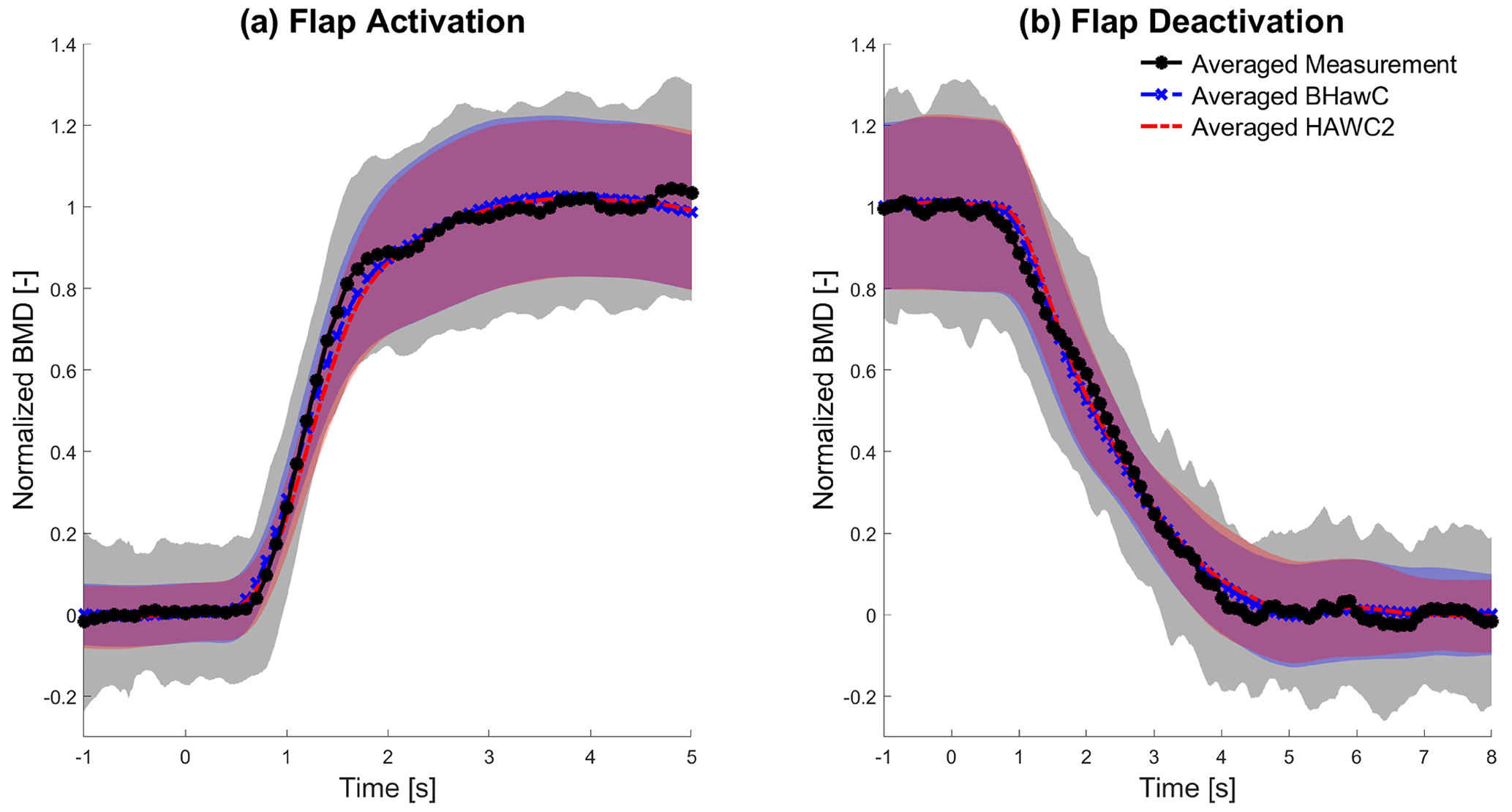
Figure 12 Comparison of the normalized averaged b2b blade root bending moment (BMD) transient curve obtained from all BHawC (blue dashed line with x marker) and HAWC2 (red dash-dotted line) simulations and all measurements (black line with asterisk marker) during flap activation (a) and deactivation (b), including an error band of 1 SD of the matching colors.

Figure 12a shows the comparison of the average BMD transient curve during flap activation of the measurements (black line with asterisk marker), BHawC simulations (blue dashed line), and HAWC2 simulations (red dash-dotted line) based on all the available data. The simulation curves are almost equivalent, with a maximum time shift within 0.6 s (less than three time steps), keeping the maximum load difference within 5 % of the ΔBMD. The transient curves also differ from the curves obtained in the initial validation. The load keeps increasing and fluctuates after the flap's full activation, a behavior also shown by the measurement transient. This behavior is probably caused by averaging the load difference obtained from all the different wind conditions. The simulation curves are well within the error band of measurement transient, with a maximum difference below 50 % of the measured SD and below 10 % of the ΔBMD due to the flap activation. Similar to the initial validation, the simulation curves start to increase earlier (around 0.1 s, 5 % of the actuation time of 2 s) but with a lower slope, underpredicting the load increase in the second half of the flap activation and accumulating a delay of 0.2 s (10 % of the actuation time) and then converging within the measured oscillating transient curve. As observed in the initial validation, the simulations cannot reproduce the S-shaped behavior the measurements manifest.

Figure 12b compares the average BMD transient curves during flap deactivation. The simulation curves differ by less than 3 % of the ΔBMD, with a maximum time shift within 0.08 s (four time steps). The simulation curves are well within the measured error band, with a maximum difference below 60 % of the measured SD and below 15 % of the ΔBMD. The simulation transient decreases 0.2 s (4 % of the 4.5 s deactivation time) later than the measured curve, but they quickly converge within the measurement oscillation curve.

During the actuator model tuning, the flap displays a slower activation and a faster deactivation when the wind turbine is in normal operation compared to the idling state. This behavior suggests that the aerodynamic loading on the blade section may influence the deflection of the flap. To investigate this hypothesis, the averaged BMD transient curves are computed for wind speed intervals with a 2 m s⁻¹ range, a wind interval with expected similar aerodynamic load values. The averaged transient curves are shown in Fig. 13 for flap activation and Fig. 14 for flap deactivation. For wind speed intervals up to 13 m s⁻¹, the simulated transient curves closely resembled the corresponding measured curves, exhibiting differences similar to those observed in the global transient curves. The data are scarce for the intervals above 13 m s⁻¹, resulting in irregular and oscillating transient curves. From the comparison of the measured averaged curves shown in Fig. 15a for flap activation and Fig. 15b for flap deactivation, a correlation between the wind speed and the transient curve does not emerge clearly. The measured transients all lie within a range of 0.2 s in both the activation and deactivation phases without a clear relation to the aerodynamic loads.

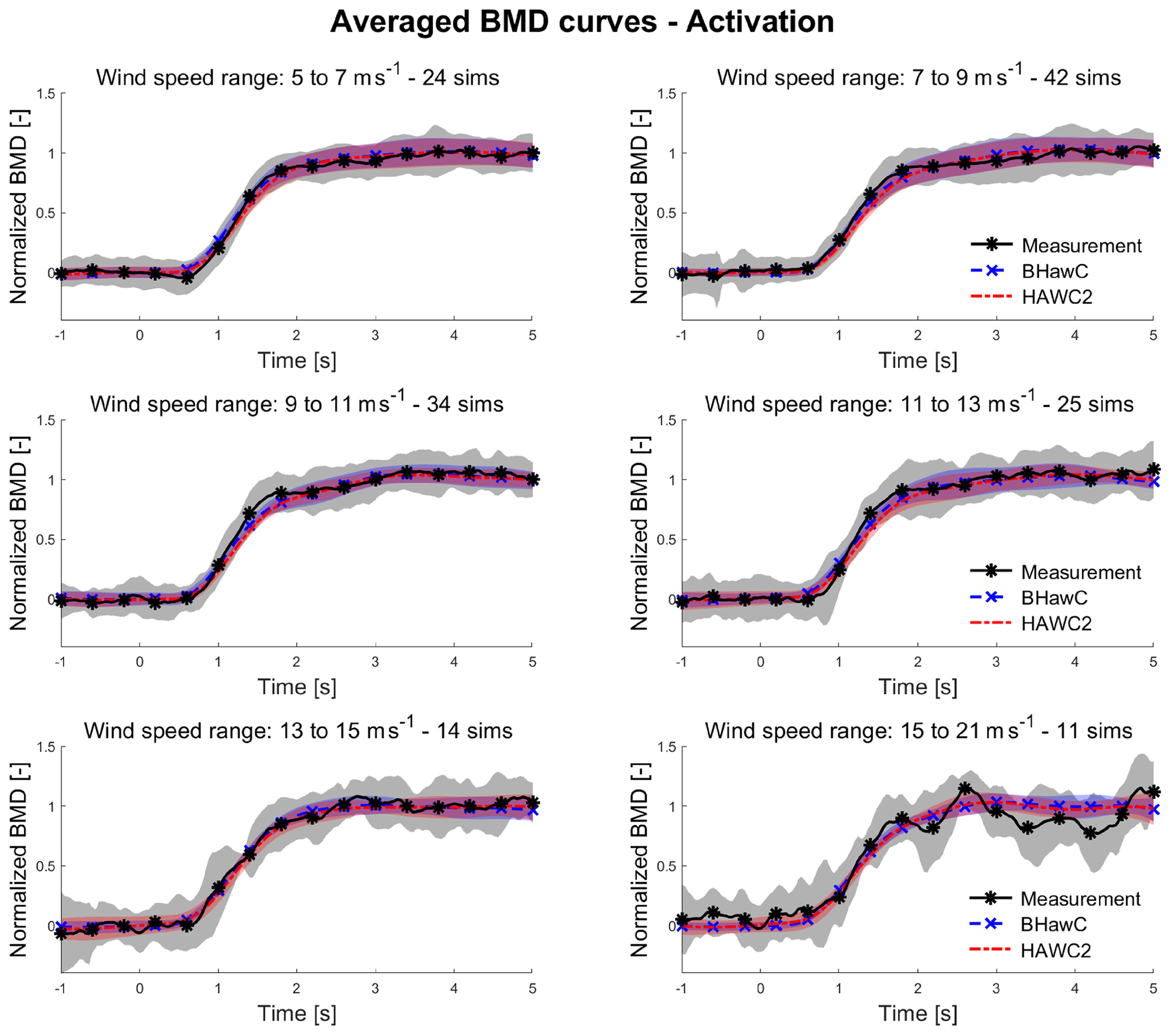
Figure 13 For BHawC (blue dashed line with x marker), HAWC2 (red dash-dotted line), and measurements (black line with asterisk marker), averaged BMD transient curves obtained for wind speed intervals of 2 m s⁻¹ during flap activation. The number of data points (sims) per wind interval is also specified.

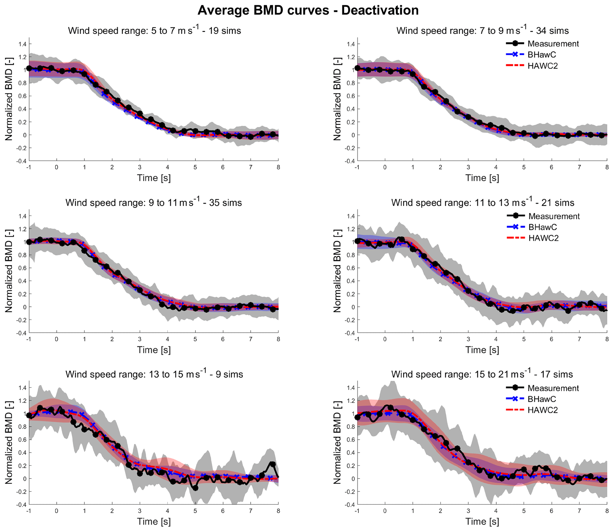
Figure 14 For BHawC (blue dashed line with x marker), HAWC2 (red dash-dotted line), and measurements (black line with asterisk marker), averaged BMD transient curves obtained for wind speed intervals of 2 m s⁻¹ during flap deactivation. The number of data points (sims) per wind interval is also specified.

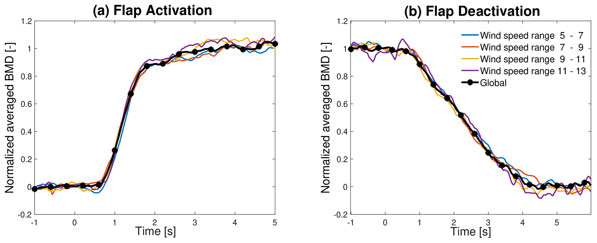
Figure 15 Comparison of the measured BMD transient curves obtained for different wind speed intervals for flap activation (a) and flap deactivation (b).

7 Near-wake model study

In the ATEF model validations described in the previous sections, as well as in the stationary validation of the same ATEF models described in Gamberini et al. (2022), the aeroelastic codes did not model the 3D effects originated by the vorticity trailed from the edges and along the span of the flap section. The HAWC2 code can account for these 3D effects via the optional near-wake induction model at the cost of higher model and computational complexity. This model, introduced by Pirrung et al. (2017), is a simplified version of the lifting line model specifically designed to examine the wake near each blade. The near-wake model accounts for the temporal evolution of the trailed vorticity. The vorticity is traced between all the aerodynamic sections on the blade, allowing the model to capture various vortices, such as tip and root vortices. Furthermore, the model considers vorticity trailed at the edges of flaps and vorticity resulting from radial load fluctuations in turbulent inflow. The strength of the trailed vortex at each trailing point is determined by computing the disparity in bound vorticity between adjacent aerodynamic blade sections. This calculation incorporates an approximation of the buildup of unsteady circulation.

Prospathopoulos et al. (2021) showed that the near-wake induction model improves the prediction of the flap's local and global impact on the thrust forces. These changes in flap performance are investigated by performing the initial and extended validations also with the near-wake model enabled in HAWC2 (HAWC2-NW). The near-wake model impacts the ΔCl at the analyzed flap location, reducing the increase in Cl during flap actuation of 7 % compared to the HAWC2 results without the near-wake model. The averaged Cl transient curves differ by less than 3 % of the ΔCl during flap activation, mainly due to a time shift of almost two time steps, and less than 4 % of the ΔCl (time shift around three time steps) during flap deactivation. The near-wake model reduces the ΔBMD of the flap actuation between 2 % and 2.5 %. Meanwhile, the HAWC2-NW BMD transient curve is almost equivalent to the HAWC2 curve, with a difference below 1 % of the ΔBMD during flap activation and below 0.6 % of the ΔBMD during flap deactivation.

8 General discussion

The validations described in Sects. 5 and 6 show the HAWC2 and BHawC aeroelastic models of the ATEF implemented on the Prototype provide almost equivalent results during the flap activation and deactivation. In the initial validation based on the blade section measurements, the respective HAWC2 and BHawC Cl transients have a time shift below 0.04 s, leading to a maximum difference lower than 6 % of the ΔCl occurring during flap actuation. In the extended validation, the simulated b2b load transients differ by less than 5 % of the ΔBMD caused by the flap actuation, with the difference mainly originating by a maximum time shift of 0.1 s.

The validations proved that the simulations are in good agreement with the measurements. The simulated average Cl transient curves are well within the error band of the measured curves, with a maximum difference below 8 % of the ΔCl during flap activation and deactivation. The differences between the simulated and measured average BMD transient curves are below 10 %. Within this error margin, the simulations cannot completely reproduce the average transients' shape, especially during the flap actuation, where the measurements rise later but steeply, reaching full activation value earlier. The main proposed causes of this difference in the transient shape are as follows.

• Incomplete flap deflection model. The actuator model is tuned with the flap deflections measured only at one wind speed. The flap deflection transients may vary as the external conditions, like aerodynamic forces or the rotational speed, change. As shown in Fig. 15, there is no clear correlation between the BMD transient curves from different wind speed intervals and the wind conditions. However, the differences between the averaged curves have a magnitude comparable to the validation error margin, suggesting that the variation in the external conditions can partly justify the differences observed between simulations and measurements. Furthermore, the flap deflection data were measured only at one blade section, which does not ensure the flap has a constant deflection along its whole 20 m length. A spanwise variation in the flap deflection could justify the steeper shape of the BMD transient. Additional measurements of the flap deflection at different blade locations, wind speeds, and wind turbine operative conditions can improve the deflection model, reducing the transient shape difference.

• Accuracy of aerodynamic properties for airfoils including flap. The Cl and Cd curves used in the aeroelastic simulations were all derived from the wind tunnel measurement of the 21 % thickness airfoil. New wind tunnel measurements for the 18 % and 24 % airfoils and different relative sizes of flap and chord can verify if the flap airfoils' aerodynamic properties are correct or responsible for the observed difference in the transient curves' shape.

• Uneven distribution of the azimuthal angle at flap actuation time in the measurements. The Cl and BMD transient are strongly affected by the azimuthal angle at which the flap actuation is initiated, as shown in Sect. 5. In the available measurements, the azimuthal angle at flap actuation was not evenly distributed on the whole rotor, leading to a distorted averaged transient. In the one-to-one process, this was partly compensated for by simulating the flap activation at the measured azimuthal angle at flap actuation. Additional measurements aiming to balance the distribution of this angle at all wind speeds can potentially improve the quality of the measured transient curves and reduce the difference between measurement and simulation.

• Incomplete flap aerodynamic model. The transient curve difference can suggest a delay of the change in aerodynamic flow compared to the flap actuation, a delay dependent on the flap position (as it is not present during flap deactivation) that is quickly recovered during the activation. CFD simulations modeling the exact geometry of the flap deflection can verify this hypothesis.

Based on the experience gained in the validations presented in this paper, some recommendations are suggested to improve future validation campaigns of active flaps:

• The correct estimation of the flap deflection is crucial in the validation of the aerodynamic model of the ATEF. If continuous measurements of the flap position are unavailable, the deflection curve should be measured for several wind and operative conditions to ensure the correct tuning of the actuator model.

• Uncertainties about the aerodynamic properties of the flap airfoils reduce the accuracy at which the aerodynamic model can be validated. Proper measurements of all the relevant flap airfoils should be conducted. If that is not possible, the Cl and Cd impact of the flap can be derived from similar airfoils with acceptable accuracy.

• The correct time synchronization of all the different measurement systems is crucial to ensure the proper time precision in measuring and validating the transient curves of the Cl and load signals. Therefore, the flap actuator control (or any other channel that can be used to estimate the flap actuation time) is required.

• The azimuthal angle at which the flap is actuated strongly affects the transient curve of Cl and loads. The measurement campaign should aim to obtain measurements with a balanced distribution of these angles.

In Sect. 7, the HAWC2 near-wake induction model (model accounting for the 3D effects due to the vorticity trailed from the edges and along the span of the flap section) does not affect the average transient of ΔCl and ΔBMD as they differ respectively less than 4 % and 1 % compared to the HAWC2 model without near wake. The near-wake model impacts the value of ΔBMD marginally, reducing it between 2 % to 2.5 %. This reduction, even if small, improves the model's accuracy to estimate the ΔBMD as the HAWC2 model overestimates it, as shown in Gamberini et al. (2022). This result confirms the conclusions of Prospathopoulos et al. (2021), which are that a BEM model without 3D trailed vorticity effects overestimates the flap contribution at the flap location and the blade root. However, the difference in the integral loads is rather small when the flap actuation frequency is below 1 P, like in the validation described in the current paper.

Finally, the azimuth-based b2b method proved to be a reliable methodology to estimate the asymmetrical loading caused by the ATEF equipped on a single blade of the Prototype. This methodology can be applied in other asymmetrical rotor loading conditions, for example, in the case of individual pitch, pitch error, or blade degradation.

9 Conclusions

Within the framework of the VIAs project, an active trailing edge flap system was installed on a 4.3 MW test wind turbine and underwent a field test campaign for over 1.5 years. The campaign provided the measurement data to validate the aerodynamic ATEF model of the aeroelastic engineering tool BHawC and the more advanced ATEFlap model of HAWC2. The validation focused on the dynamic response of the ATEF models during flap actuation and consisted of three phases. At first, the flap actuator model was tuned to accurately reproduce the flap deflection during the 2 s activation and the 5 s deactivation. In the second phase, the aerodynamic flap model was tuned and validated through the lift coefficient transient responses measured at a blade section equipped with the flap. Finally, the aeroelastic ATEF model was validated under varying weather conditions based on the blade load transient responses over 3 months, from October to December 2020. A novel approach to computing the blade load impact of the flap was introduced. This method is an azimuth-based variation in the blade-to-blade approach, and it computes the difference between azimuthal synchronized loads of adjacent blades.

The validation showed that for the tested actuator model, the two aeroelastic ATEF models provide almost identical transients during flap activation and deactivation, with the main difference caused by a relative time shift lower than 0.04 s (two time steps) between the Cl transients and below 0.08 s between the load transients. The validation showed that the simulation transient responses of Cl and BMD are in good agreement with the corresponding measured responses, confirming that the aeroelastic ATEF models provide a reliable and precise estimation of the impact of the flap on the wind turbine during flap actuation. In comparison with the field data, the maximum differences between the simulated and the measured Cl transient curves are below 8 % of the ΔCl and within 0.15 s of time shift during flap activation and below 8 % of the ΔCl and within 0.2 s of time shift during flap deactivation. Regarding the BMD transient curves, the maximum difference is below 1 % of the mean blade load during flap activation and below 1.7 % during flap deactivation, with a delay within 0.2 s for both flap actuation cases. Additional measurements of the flap deflection at different blade locations, under wide wind turbine operational conditions, and the direct measurement of the aerodynamic properties of all flap airfoils are suggested solutions to fine-tune the ATEF model.

To the authors' knowledge, this validation is the most extensive published study of the aeroelastic ATEF model transient responses in terms of wind conditions, time, and flap size. This validation was enabled by measuring the aerodynamic response at a blade section during flap activation/deactivation with a unique inflow and pressure belt system. Combined with the complementary validation of the static properties of the aeroelastic ATEF model, this validation increases the safety and reliability of the aeroelastic design environment for the wind turbine equipped with active flaps. It provides a validated and reliable foundation for further exploration of the ATEF technology, a fundamental milestone in designing future wind turbines equipped with ATEFs. Future research should aim to identify the limits of application of the ATEF models in terms of, for example, actuator performance (e.g., maximum speed or deflection) or external conditions (e.g., wind misalignment, extreme wind speed, or direction change).