Wind tunnel investigations of an individual pitch control strategy for wind farm power optimization

This article presents the results of an experimental wind tunnel study which investigates a new control strategy named Helix. The Helix control employs individual pitch control for sinusoidally varying yaw and tilt moments to induce an additional rotational component in the wake, aiming to enhance wake mixing. The experiments are conducted in a closed-loop wind tunnel under low-turbulence conditions to emphasize wake effects. Highly sensorized model wind turbines with control capabilities similar to full-scale machines are employed in a two-turbine setup to assess wake recovery potential and explore loads on both upstream and downstream turbines. In a single-turbine study, detailed wake measurements are carried out using a fast-response five-hole pressure probe. The results demonstrate a significant improvement in energy content within the wake, with distinct peaks for clockwise and counterclockwise movements at Strouhal numbers of approximately 0.47. Both upstream and downstream turbine dynamic equivalent loads increase when applying the Helix control. The time-averaged wake flow streamwise velocity and rms value reveal a faster wake recovery for actuated cases in comparison to the baseline. Phase-locked results with azimuthal position display a leapfrogging behavior in the baseline case in contrast to the actuated cases, where distorted shedding structures in the longitudinal direction are observed due to a changed thrust coefficient and an accompanying lateral vortex shedding location. Additionally, phase-locked results with the additional frequency reveal a tip vortex meandering, which enhances faster wake recovery. Comparing the Helix cases with clockwise and counterclockwise rotations, the latter exhibits slightly higher gains and faster wake recovery. This difference is attributed to Helix' additional rotational component acting in either the same or the opposite direction as the wake rotation. Overall, both Helix cases exhibit significantly faster wake recovery compared to the baseline, indicating the potential of this technique for improved wind farm control.

1 Introduction

The growing demand for renewable energy sources has led to the increased deployment of wind turbines in many parts of the world. However, the power output of wind turbines can be significantly impacted by the complex flow dynamics in their wakes. The reduction in the incoming wind velocity and increased turbulence caused by the wake can reduce the efficiency of downstream turbines, limiting the overall power output of a wind farm. Therefore, understanding and controlling the wake behavior is critical to enhance the efficiency of wind farms and increase their power output. Therefore, wind farm control is identified as being important for fulfilling the main challenges in wind energy science stated by Veers et al. (2019). The last decades' vast research was directed at understanding the wake and applying different techniques to control it with various aims, from power optimization to load reduction. A comprehensive review of recent wind farm flow control strategies was published by Meyers et al. (2022).

Lately, wake-mixing techniques, which aim at enhancing recovery by perturbing the wake at specific frequencies attracted the attention of the research community. In the literature, several control strategies that aim to influence the turbulent mixing of wind turbine wakes are presented. An example of such a control strategy is to periodically change the yaw misalignment with respect to the incoming wind, which results in bending perturbations in the wake that lead to a faster recovery. This was investigated numerically by Kimura et al. (2019), who showed the potential of this technique. In another study Munters and Meyers (2018a) showed that a dynamic turbine excitation triggers wake meandering. Moreover, they showed that this effect is decreased for increasing turbulence intensity. Dynamic induction control (DIC), where the induction factor is dynamically varied by a combination of pitch and torque control is another possibility to enhance wake mixing. In this way, axial perturbations are generated in the wake. This control strategy was investigated numerically by Munters and Meyers (2017) and Yılmaz and Meyers (2018) and also experimentally by Frederik et al. (2020b). However, these studies show that the application of this technique results in increased dynamic loads on the downstream turbines. Furthermore, Munters and Meyers (2018b) suggest that it is only efficient applying such a technique to first-row turbines in low-turbulence conditions. The loads on the upstream and downstream turbine should be limited by another way of dynamically influencing the wake by mixing, which is termed the Helix approach, introduced by Frederik et al. (2020a). In the Helix approach, individual pitch control (IPC) is used to sinusoidally change the blade pitch, resulting in a variation in the fixed-frame tilt and yaw moments. Consequently, an additional excitation of the wake is introduced. In their computational fluid dynamics (CFD) study, Frederik et al. (2020a) explain the concept of the Helix technique and show the meandering of the wake and the potential for enhanced wake mixing. In another numerical study, Frederik and van Wingerden (2022) investigate the influence of DIC and Helix on the tower and blade loads. They show that both wake-mixing techniques increase the loads of upstream and downstream turbines, whereas the Helix approach has a higher effect on the turbine blades than on the tower. The authors conclude that despite the increased loads, wake-mixing techniques are an option for full-scale applications. A CFD analysis was conducted by van den Berg et al. (2022) to evaluate the effect of the Helix approach applied to floating wind turbines. Their results suggest that the Helix control strategy can even be more efficient when applied to floating turbines compared to bottom fixed machines. In a more recent study, Taschner et al. (2023a) perform large-eddy simulations of a two-turbine wind farm and check the effect of various pitch amplitudes. They find an increasing mixing effect with increasing pitch angles showing no saturation in the investigated pitch angle range, which reaches up to pitch angles of 6°. Furthermore, they show the occurrence of increasing loads when increasing the pitch amplitudes, suggesting an optimal operation of the Helix as a trade-off between power gain and loading. Since most of these studies focus on the numerical investigation of the Helix approach, a thorough experimental verification cannot be found to date. For this reason, this study investigates the potential of the Helix approach experimentally in a wind tunnel (W/T) and should give a detailed insight into the wake aerodynamics. To provide such a detailed insight, the flow in the wind tunnel has to be a clean lab flow which is uniform and is characterized by a very small turbulence intensity. Such clean inflow will not only highlight the effects of the control technique in the wake but also influence their effectiveness. Wake-mixing techniques like Helix add turbulence to the wake. Consequently, if the turbine inflow is already characterized by higher ambient turbulence, the effect of wake mixing will be mitigated. In a recent study Mühle et al. (2024) compare power gains for wake mixing by dynamic yaw for different inflow turbulence. They found a strong reduction in the effect on the power of a two-turbine setup in the case of high inflow turbulence and thus confirm the findings of Munters and Meyers (2018a). Nevertheless, they suggest that wake mixing has the potential to improve the power output of a wind farm in the case the wakes are strong and persistent.

This present study is guided by two research questions. Firstly, the effects of the Helix approach are examined, focusing on both the turbine-level observations and the fluid flow in the turbine wake. This will allow an assessment of whether Helix can enhance the entrainment of incoming wind flow and improve the efficiency of power extraction in wind farms. Secondly, the identification of the underlying mechanisms in the wake that lead to faster wake recovery are investigated. This will provide insights into the complex flow dynamics behind wind turbine wakes and the role that Helix plays in modifying these dynamics. Understanding these flow mechanisms is critical to optimize the use of Helix in wind farm design and operation. By addressing these research questions, a contribution to the development of more effective control strategies for wind turbines and a deeper understanding of the flow dynamics in wind turbine wakes should be achieved.

To address the research questions outlined above, a methodology that combines wind tunnel (WT) experiments with detailed wake analyses is applied. At first, turbine-level experiments to study the effects of the Helix approach on the wind turbines in tandem configuration are conducted. This involves installing sensors on the wind turbine to measure its performance and analyzing the data to assess the impact of the Helix strategy on power output and experienced loads. This allows an assessment of the performance of the wind turbine under different Helix control conditions and identifies any improvements resulting from the application of Helix. Finally, a detailed wake analysis to identify the mechanisms in the wake leading to faster wake recovery is carried out. This involves analyzing the mean flow field as well as phase-locked flow structures behind the wind turbine in order to provide an understanding of the effects of Helix on the performance of wind turbines and the complex flow dynamics in their wakes.

In the following sections, the control strategy (Sect. 2) – the Helix approach – and the experimental setup (see Sect. 3) will be described in detail, with emphasis on the advanced techniques employed for data acquisition and processing. In the section on the wind tunnel results, Sect. 4, the turbine-level results will be presented and analyzed first, identifying interesting excitation strategies for further investigation. The wake study results will be presented in two parts – a time-averaged wake analysis and detailed phase-locked studies of the tip vortex area. Here, the discussion deals with the interpretation of the results and shows implications for wind turbine design and operation. Finally, the conclusions and outlook in Sect. 5 will summarize the key findings and their significance, as well as offer an outlook for further research and development of control strategies in wind turbine technology.

2 Individual pitch control: the Helix approach

In order to optimize the power output of wind farms, it is essential to understand the aerodynamics of the wind turbine wake. The low-speed region governing the wake is the reason that multiple successive wind turbines need to be separated with a certain spatial distance between them. By controlling the upstream turbine wake, e.g., introducing additional instabilities into the flow, synergetic effects on the entire wind turbine farm can be achieved. Hence, controlling and influencing the wake recovery has a huge potential for wind farm power optimization. Basically, the flow behind a wind turbine is defined by the continuous sheet of vorticity which rolls up to two bigger vortices: the tip vortex and the root vortex. The root vortex imposes a rotary movement on the wind turbine wake that is counter-rotating to the turbine rotation. The tip vortices build a helical system in the wake of the wind turbine. The wake aerodynamics can be separated into three main phenomena: the vortex shedding, the tip vortex pairwise instability (also known as leapfrogging instability), and the turbulent mixing (see Lignarolo et al., 2015, Sarmast et al., 2014, and Sørensen, 2011). If it is possible to influence the tip vortex breakdown, and thereby increase the net entrainment of kinetic energy, the wake can be re-energized and, therefore, recover earlier. The predominant instability mode in wind turbine wakes is the mutual inductance instability, where adjacent helical filaments influence each other and start to roll up, which results in the leapfrogging phenomenon (Lignarolo et al., 2015).

A control strategy, taking these mechanisms into account, was introduced by Frederik et al. (2020a). In the so-called Helix approach, the wind turbine blades experience a dynamic individual pitch control/excitation (DIPC), resulting in a variation in the fixed-frame tilt and yaw moments and a dynamic variation in the direction of the thrust force. Thereby, they show a meandering of the wake in either a clockwise (CW) or counterclockwise (CCW) direction, depending on the slightly out-of-sync excitation frequency. In their proof of concept, Frederik et al. (2020a) show the potential of this technique and demonstrate that if it is applied, a faster wake recovery is detected. However, in the literature, only results of computational simulations are present so far. For this reason, in this article, the potential of the Helix approach is experimentally investigated in a wind tunnel (W/T) and should give insight into the wake aerodynamics.

In the following, the dynamic individual pitch control strategy, which was implemented in the model wind turbines to achieve a sinusoidal variation in the fixed-frame tilt and yaw moments and consequently a dynamic variation in the thrust force direction, will be explained.

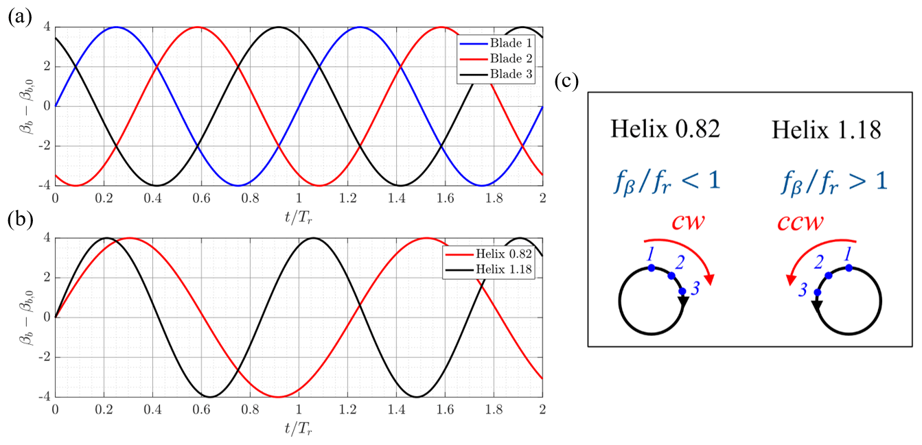
Figure 1 (a) Blade pitch for all three blades for f_r=1 P, (b) blade pitch of blade 1 for f_r<1 P and f_r>1 P with $\widehat{\mathit{\beta }}=\mathrm{4}\mathit{°}$ as a function of the normalized time $t/T_{\mathrm{r}}$, and (c) explanation of the Helix directions.

The turbine was controlled by individual pitch control (IPC), where each blade experiences a pitch excitation that varies with the azimuthal position. This is shown schematically for the excitation with the rotational frequency $f_{\mathrm{r}}={\mathit{\omega }}_{\mathrm{r}}/\mathrm{60}=\mathrm{1}\mathrm{P}$ in Fig. 1a. This is in contrast to collective pitch control (CPC), where each blade experiences the same pitch excitation at the same time.

In the case of a clean lab flow (low turbulence intensity Tu < 0.5 %, no shear), a sinusoidal variation in the fixed-frame tilt and yaw moments is assumed to be achieved by a sinusoidal variation in pitch amplitudes. A proof of this assumption will be given in Sect. 4.1. As a result, in the present study, the pitch angle β_b(t) amplitudes served as input for the controller. The blades are individually controlled with a sinusoidal excitation with a frequency $f_{\mathit{\beta }}=f_{\mathrm{r}}\pm f_{\mathrm{e}}$ which is out of sync with the rotational frequency f_r=1 P. The additional excitation frequency f_e is either added to or subtracted from the rotational frequency, leading to the CCW or CW wake meandering, respectively.

Blade pitch signals for the two cases, f_β<1 P (Helix 0.82) and f_β>1 P (Helix 1.18), are visualized in Fig. 1b for a fixed blade pitch offset ${\mathit{\beta }}_{\mathrm{b},\mathrm{0}}=\mathrm{0}\mathit{°}$.

The following equation shows the transient blade pitch angle β_b(t) for each of the three blades $b=\mathit{\{}\mathrm{1},\mathrm{2},\mathrm{3}\mathit{\}}$:

$$\begin{array}{}\text{(1)}& {\mathit{\beta }}_{\mathrm{b}}\left(t\right)={\mathit{\beta }}_{\mathrm{b},\mathrm{0}}+\stackrel{\mathrm{\Delta }\mathit{\beta }}{\overbrace{\widehat{\mathit{\beta }}\cdot \sin (\mathrm{2}\mathit{\pi }\underset{f_{\mathit{\beta }}}{\underbrace{(f_{\mathrm{r}}\pm f_{\mathrm{e}})}}t+{\mathit{\theta }}_{\mathrm{b},\mathrm{0}})}}.\end{array}$$

Here, the blade pitch excitation amplitude is denoted as $\widehat{\mathit{\beta }}$, the respective blade pitch offset β_b,0, and the azimuthal blade position ${\mathit{\theta }}_{\mathrm{b},\mathrm{0}}=-(\mathrm{2}\mathit{\pi }/\mathrm{3})\cdot (b-\mathrm{1})$ at t=0 s. Since, the G1 model is three-bladed, the azimuthal blade positions are ${\mathit{\theta }}_{\mathrm{1},\mathrm{0}}=\mathrm{0}\mathit{°}$, ${\mathit{\theta }}_{\mathrm{2},\mathrm{0}}=-\mathrm{120}\mathit{°}$, and ${\mathit{\theta }}_{\mathrm{2},\mathrm{0}}=-\mathrm{240}\mathit{°}$.

In the case f_e is subtracted, $f_{\mathit{\beta }}/f_{\mathrm{r}}$ will be smaller than 1 (Helix 0.82). Consequently, the additional rotation will be in the same rotational direction as the rotor, as one pitch period is longer than one rotation period of the rotor. This is schematically shown in Fig. 1c for a clockwise-rotating turbine, where the blue line indicates the turbine rotation and the red line indicates the additional rotation for three pitch periods. In contrast, in the Helix 1.18 case (adding f_e), the pitch period is shorter than the rotor rotation, and thus the additional rotation is in the opposite direction of the rotor rotation.

To be able to better compare the Helix excitation methodology with other dynamic control strategies, the additional frequency f_e can also be expressed in terms of the Strouhal number, correlating the additional excitation frequency f_e with the blockage-corrected inflow velocity U_∞,corr. It is calculated as $S{t}_{\text{add}}=\frac{f_{\mathrm{e}}D}{U_{\mathrm{\infty },\text{corr}}}$, where D is the rotor diameter. In this way the Strouhal numbers will be identical if the same f_e is added or subtracted, and the difference will be indicated by specifying a CW or CCW rotational direction. In the article, values for both notations $f_{\mathit{\beta }}/f_{\mathrm{r}}$ and St will be provided.

3 Experimental setup

In the following section, the experimental setup of the wind turbine model tests conducted in the boundary layer wind tunnel at the Technical University of Munich (TUM) is described. The section is separated into giving details on the model wind turbines, the wind tunnel itself, and the measurement stages.

3.1 Model wind turbines

For the wind tunnel tests, two identically scaled wind turbine models are arranged in a tandem configuration. The rotor diameter of the machines, depicted as G1 models in the following, is D = 1.1 m. A detailed description of the G1s is given by Bottasso and Campagnolo (2021). Nevertheless, a brief summary of the applied sensors and controls is given in the following. The operating rotor speed of the three-bladed G1 is 840 rpm. The blades are manufactured out of unidirectional carbon fiber. Each blade is equipped with an individual pitch actuator and a built-in relative encoder measuring the pitch angle. The rotor azimuthal position θ is detected via an optical encoder. Furthermore, a torque meter can measure the torque in front of the torque generator. Moreover, full-bridge strain gauges are used to measure the torque and the two out-of-plane bending moments on the rotating shaft between the rotor and the front bearing. Similarly, sensors located at the tower base allow measuring the fore–aft and side–side bending moments therein. Finally, nacelle nodding and yawing bending moments are derived by projecting the shaft rotating loads into a fixed-axis system. The G1 model is controlled with an industrial real-time Bachmann M1 controller that samples the azimuth and the rotating loads every 0.4 ms and all other quantities (e.g., tower loads and blade pitch) every 4 ms. The controller is connected to a supervisory PC, where all settings and recordings concerning the wind turbine can be done. The control algorithm for the Helix strategy is implemented in the turbine controller. While the rpm is kept fixed at an optimum value throughout the experiments, the demanded blade pitch is varied according to Eq. (1).

3.2 Wind tunnel

The wind tunnel experiments are carried out in the closed-loop (Göttingen-type) low-speed wind tunnel C (W/T-C) of the Chair of Aerodynamics and Fluid Mechanics of the Technical University of Munich (TUM-AER). Besides power measurements of the wind turbine itself, transient fast-response five-hole pressure probe measurements in the wake of the wind turbine model are intended. The W/T-C closed test section has a size of 1.8 × 2.7 × 21.0 m³ (height × width × length). The ceiling of the wind tunnel is adjustable to minimize the pressure gradient in the longitudinal direction. Turbulence intensity lies below Tu < 0.5 %. In general, in order to simulate the atmospheric boundary layer as seen in the real-world case, it is possible to equip the wind tunnel with a vortex generator and roughness elements. Nevertheless, in this study, the boundary layer instrumentation is omitted in order to emphasize the aerodynamic effects of the Helix actuation while operating the wind tunnel with low turbulence intensity. The blockage ratio $\mathit{\alpha }=A_{\text{turbine}}/A_{\text{wind\hspace{0.17em}\hspace{0.17em}tunnel}}$ in the experiment lies at α=0.2, which is rather high. To account for this blockage effect, the wind tunnel free-stream velocity was adjusted to U_∞≈ 5.3 m s⁻¹, which is lower than the rated wind speed of the G1 models (Bottasso and Campagnolo, 2021). As a result of the blockage, the fluid is however accelerated, resulting in a higher velocity experienced by the turbines. To account for such an effect on the turbine performance, it can be corrected by applying analytical models, and a recent review is presented in the study by Steiros et al. (2022). More information is presented by Ross and Polagye (2020), who conducted an experimental assessment of such models and their application to different wind turbine concepts. In the present study, the performance was corrected by a calculation of the rotor effective wind speed (REWS) for the upstream G1, done as described in Campagnolo et al. (2022). This revealed a blockage-corrected free-stream velocity $U_{\mathrm{\infty },\text{corr}}\approx$ 5.9 m s⁻¹, which correlates to the rated wind speed of the model wind turbine. Consequently, the turbine is operated at a tip speed ratio of approx. λ=8.2. Based on the authors' knowledge, there are no analytical blockage correction models that would allow us to quickly assess the influence of the wind tunnel walls on the wake. One possible way to investigate this is to use computational fluid dynamics (CFD). Zaghi et al. (2016) studied the effect of blockage on a model wind turbine with a Reynolds-averaged Navier–Stokes (RANS) simulation. They analyzed the streamwise wake velocity and found increased velocities in the area behind the rotor but also in the outer region of the wake in the case a wind tunnel wall was present. In a more detailed analysis Sarlak et al. (2016) used large-eddy simulation (LES) combined with the actuator line technique to investigate wake velocity and Reynolds stresses for different blockage ratios up to α=0.2. They found a significant impact on the mean wake velocity in the case of the highest blockage ratio. Especially in the region outside of the rotor, the velocity is found to increase; this augmentation is mitigated in the rotor area but is still present. Furthermore, they concluded that blockage has no considerable effect on the wake mixing rate as maximum and minimum velocities do not differ significantly. In a combined experimental and numerical study, McTavish et al. (2014) investigated the influence of wind tunnel blockage on the wake width and found that the wake compresses when blockage increases. Consequently, the wake results of the present study are expected to be characterized by slightly higher streamwise velocities and a narrower wake compared to a full-scale test. As a result, in the analysis of the measurements conducted in Sect. 4, the presence of low inflow turbulence and the rather high blockage should be considered when interpreting the results, especially when applying the findings to realistic wind turbine flows. Consequently, the data have to be seen as tendencies and not providing insight into realistic power gains of full-scale wind turbine tandem configurations.

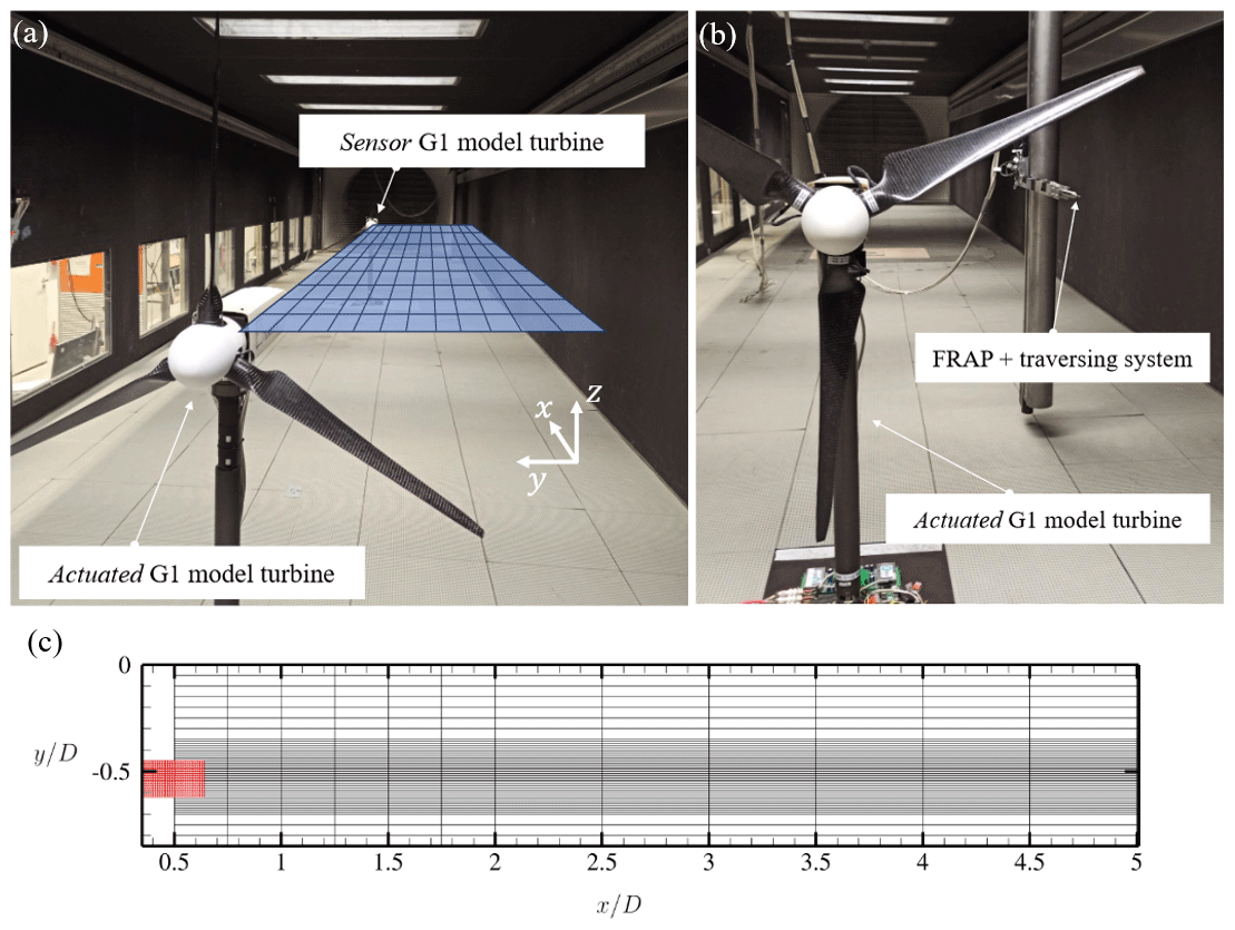
Figure 2 Wind tunnel setup for the two measurement stages: (a) two G1 wind turbine models and a schematic representation of the FRAP measurement grid and (b) one G1 turbine and the FRAP in TUM-AER W/T-C; (c) measurement grids for wake measurements (black) and refined wake measurements (red).

3.3 Measurement stages

The measurement campaign is divided into two scenarios/stages.

In the first stage (see Fig. 2a), two turbines are placed in line with a longitudinal distance of 5 D (see Fig. 2a). The upstream turbine is actuated following the control strategy introduced in Sect. 2. The downstream turbine acts purely as a sensor, providing an integral insight into the energy content in the wake and thus the recovery behind the first turbine. With this setup, a vast variety of different actuation frequencies and amplitudes can be tested in order to identify the control settings characterized by the most prominent and promising effects.

As pretests, a range of pitch amplitudes $\widehat{\mathit{\beta }}=(\mathrm{1}\mathit{°}:\mathrm{1}\mathit{°}:\mathrm{5}\mathit{°})$ were tested to investigate the capabilities of the pitch system and specifically to assess the largest achievable amplitude given the ultimate currents and pitch rate of the available actuators. As a result, within the present investigation, the Helix actuation implemented on the upstream turbine (actuated G1) is achieved with a pitch amplitude $\widehat{\mathit{\beta }}=\mathrm{4}\mathit{°}$. This control is expected to produce the greatest possible effects on the wake shed by the machine without exceeding the actuation limits.

In this study, tests were therefore conducted by solely changing the additional pitch excitation frequency f_e, which is controlled by setting a desired pitch frequency f_β in the Bachmann M1 controller. For the test with the two-turbine setup, f_β was varied within the range $\mathrm{10.1}:\mathrm{0.3}:\mathrm{17.9}\mathrm{Hz}$. In the controlled and uncontrolled configuration, the upstream turbine is operated with a constant rotational frequency of $f_{\mathrm{r}}=\mathrm{840}\mathrm{rpm}/\mathrm{60}=\mathrm{14}\mathrm{Hz}$ and an optimal collective pitch offset of β₀=0.4°. With these adjustments, the turbine operates at the desired G1 tip speed ratio λ=8.2 at $U_{\mathrm{\infty },\text{corr}}\approx$ 5.9 m s⁻¹. These controls result in a non-dimensional actuation frequency of $f_{\mathit{\beta }}/f_{\mathrm{r}}=(\mathrm{0.72}:\mathrm{0.02}:\mathrm{1.28})$, which corresponds to a Strouhal number St_add within the range $\mathrm{0}:\mathrm{0.052}:\mathrm{0.73}$ in both CW and CCW directions. For each investigated actuation frequency, the measurement time is set to t_s = 40.0 s. With this recording time and the beat frequency of f_e = 2.5 Hz, the rotation of the fixed-frame moments induced by the Helix control is recorded 100 times in one measurement interval. The downstream turbine (sensor G1) instead serves as a sensor. To this aim, it is down-rated and operates at a constant rotational velocity of f_r = 750 rpm with a pitch offset of β₀ = 0°. This rotational velocity was adjusted based on wake measurements at the location of the downstream turbine behind the uncontrolled upstream turbine so that the tip speed ratio of the sensor turbine was approx. λ=8.2. Around this tip speed ratio, the C_P−λ curve of the G1 is rather flat. Changing inflow conditions due to the Helix should therefore only have a minor impact on the power coefficient of the sensor turbine.

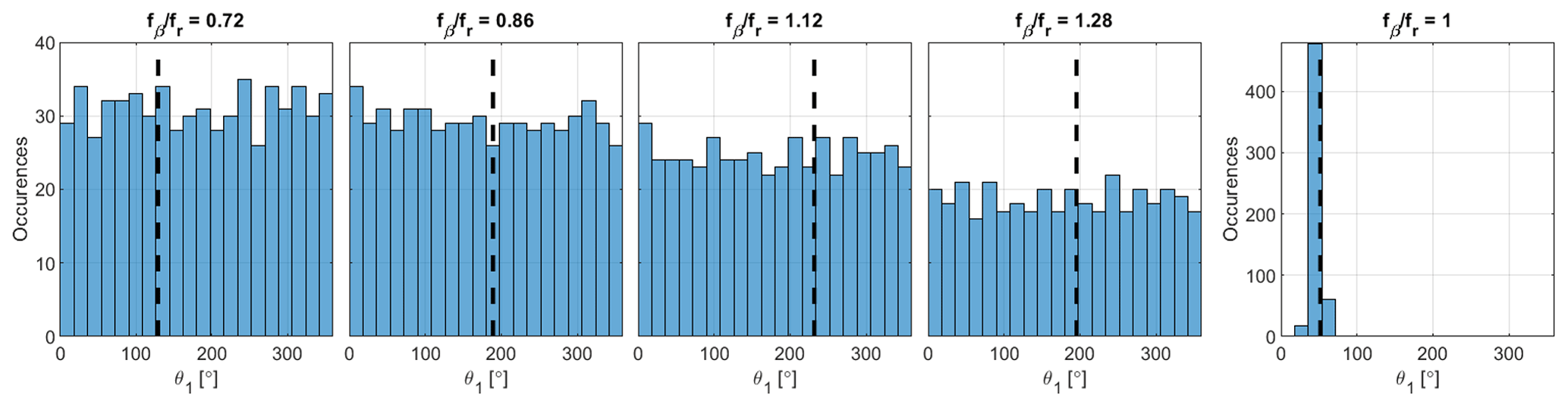
Figure 3 Distributions of the first blade azimuth (θ₁) detected when the required pitch is close to β_max and with $f_{\mathit{\beta }}/f_{\mathrm{r}}=[\mathrm{0.72},\mathrm{0.86},\mathrm{1.12},\mathrm{1.28},\mathrm{1}]$. The dashed black lines mark θ_1,ini, i.e., the azimuth position recorded at the very first time the required pitch is within the range $\mathrm{0.98}{\mathit{\beta }}_{\text{max}}<{\mathit{\beta }}_{\mathrm{1}}<\mathrm{1.02}{\mathit{\beta }}_{\text{max}}$.

During each experiment, the Helix was activated a few seconds before the start of the acquisition to allow for the downstream propagation of the new wake. The activation of the Helix, however, was not synchronized to a specific azimuth position of the rotor. For f_β≠f_r this aspect is not relevant and does not affect the results. In this regard, each plot in Fig. 3 shows, for five of the experiments conducted, the distribution of the first blade azimuth (θ₁) detected when the required pitch is within the range $\mathrm{0.98}{\mathit{\beta }}_{\text{max}}<{\mathit{\beta }}_{\mathrm{1}}<\mathrm{1.02}{\mathit{\beta }}_{\text{max}}$, with ${\mathit{\beta }}_{\text{max}}=\widehat{\mathit{\beta }}+{\mathit{\beta }}_{\mathrm{0}}=\mathrm{4}\mathit{°}+\mathrm{0.4}\mathit{°}$ the maximum requested pitch angle. The dashed black line instead marks the azimuth position (θ_1,ini) at the very first time the required pitch is within the range $\mathrm{0.98}{\mathit{\beta }}_{\text{max}}<{\mathit{\beta }}_{\mathrm{1}}<\mathrm{1.02}{\mathit{\beta }}_{\text{max}}$. For experiments conducted with f_β≠f_r, the pitch is detected around β_max for the whole range of azimuth positions (the distribution is not completely homogeneous solely due to the discrete sampling), regardless of the value of θ_1,ini. This implies that the fixed-frame moments produced by the Helix rotate over the entire range of azimuth positions, which leads to the expected effects on the wake.

Different is the case with f_β=f_r; the maximum pitch is indeed always detected at the same azimuth position, i.e., around θ_ini. Previous experimental (Campagnolo et al., 2016) and numerical (Fleming et al., 2014) investigations found that the azimuth position of maximum pitch affects the achieved amount of wake deflection. However, the study of Wang et al. (2016) revealed that the power gains observed on the downstream machine may only be a little higher than the power losses experienced by the upstream machine, at the price of a significantly increased loading of the upstream machine. In this article, it was therefore preferred to exclude the case f_β=f_r from the following discussions. A complete analysis would, indeed, require investigating the effect of the azimuth position of maximum pitch. Furthermore, previous results have shown the poor performance of this specific implementation of the Helix, thus making it uninteresting.

The results gathered by testing with the two turbines were used to identify the two control set points ($f_{\mathit{\beta }}/f_{\mathrm{r}}>\mathrm{1}$ and $f_{\mathit{\beta }}/f_{\mathrm{r}}<\mathrm{1}$) capable of triggering the fastest wake recovery, i.e., the ones inducing the largest increases in the power produced by the downstream machine.

In the second stage (see Fig. 2b), the downstream turbine is removed from the wind tunnel. To better understand the underlying physics of the Helix approach, the wake shed by the actuated G1 is traversed with a fast-response five-hole pressure probe (FRAP). Specifically, the wake is captured at hub height and along an x–y plane spanning only the right side of the turbine (see Fig. 2a). The wake measurements are performed for three different actuation cases: the reference one, characterized by $\widehat{\mathit{\beta }}$ = 0°; “Helix 0.82/CW”, with $f_{\mathit{\beta }}/f_{\mathrm{r}}=\mathrm{0.82}$ and St_add=0.47; and “Helix 1.18/CCW”, with $f_{\mathit{\beta }}/f_{\mathrm{r}}=\mathrm{1.18}$ and St_add=0.47. These two Helix cases were the ones producing the largest increase in power production for the downstream G1, as discussed in Sect. 4.1.

The measurement grid is shown in Fig. 2c. Radial mappings at hub height were taken at 13 downstream locations $x/D=[\mathrm{0.5}:\mathrm{0.25}:\mathrm{2.0},\mathrm{2.0}:\mathrm{1.0},\mathrm{5.0}]$, with $x/D=\mathrm{0}$ the position of the rotor disk. For each radial mapping, measurements were taken at unevenly spaced locations $y/D=[\mathrm{0}:\mathrm{0.05}:\mathrm{0.35},\mathrm{0.35}:\mathrm{0.01}:\mathrm{0.7},\mathrm{0.7}:\mathrm{0.05}:\mathrm{0.85}]$. In addition, a refinement region ($y/D=\mathrm{0.46}:\mathrm{0.01}:\mathrm{0.62}$ and $x/D=\mathrm{0.35}:\mathrm{0.01}:\mathrm{0.64}$) in the very near wake of the turbine, highlighted in red in Fig. 2c, is used to further investigate the vortex shedding mechanism.

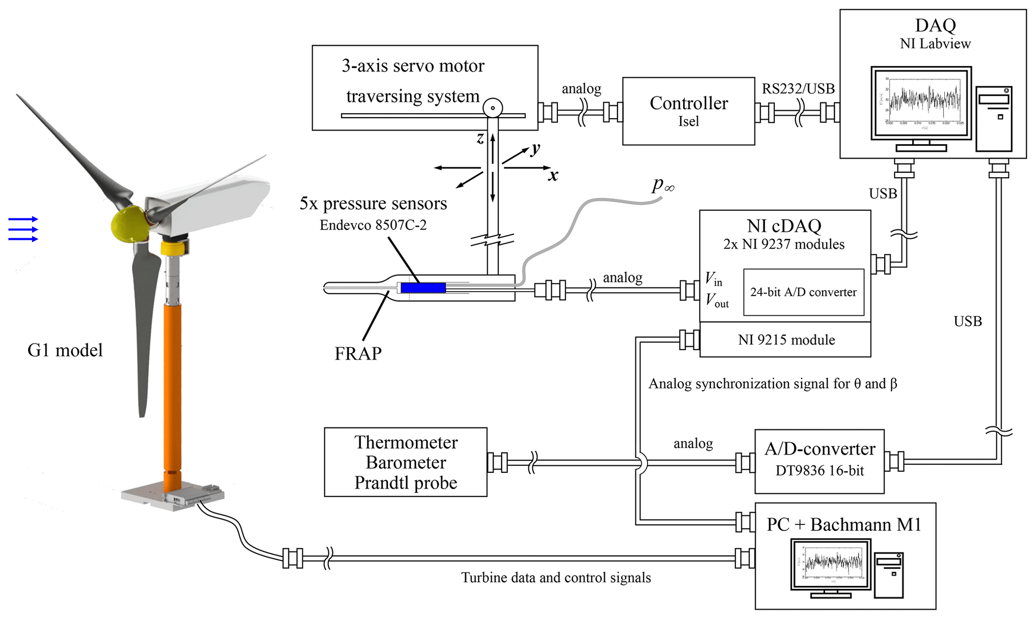
Figure 4 Schematic fast-response five-hole probe and G1 wind turbine model measurement setup for TUM-AER W/T-C.

In Fig. 4, a schematic visualization of the W/T FRAP wake measurement setup is given.

The spatial and temporal characteristics and the underlying calibration process of the FRAP can be found in the literature (see Heckmeier et al., 2019; Heckmeier and Breitsamter, 2020; Heckmeier et al., 2021; Heckmeier, 2022): a high spatial accuracy below 0.2° both in flow angles and 0.1 m s⁻¹ in the reconstructed velocity can be achieved. The spatial and temporal resolution of the applied FRAP has been investigated and hence shows the suitability of the usage of the FRAP for this experiment.

The FRAP is mounted on a three-axis traversing system. The servo traversing motors are controlled with an isel servo controller managed by LabVIEW. Moreover, the ambient air properties (static pressure p_s and temperature T_∞) and the dynamic pressure of the undisturbed inflow q_∞ are measured. The free-stream velocity is monitored with a Prandtl probe that is installed, at hub height, approx. 2 D upstream of the actuated G1 turbine. Data are acquired with a Data Translation 16-bit A/D converter. The FRAP pressure data are sampled with NI cDAQ 9237 full-bridge modules operated at a sampling frequency of f_s = 10 kHz. In order to account for aliasing problems, a low-pass filter below the Nyquist–Shannon frequency $f_{\text{LP}}\le f_{\mathrm{s}}/\mathrm{2}$ is applied in the NI cDAQ 9237 measurement card. For each position of the measurement grid, the measurement time is set to t_s = 40.0 s. In addition to the acquisition of the five pressure sensor signals, the azimuthal position θ₁ and the blade pitch β₁ of the first blade of the actuated G1 are digitized with a NI-9215 analog input cDAQ module. This allows the FRAP and wind turbine measurements to be synchronized through a dedicated postprocessing routine. Moreover, it allows the use of phase-locking techniques for a transient investigation of the full wake of the wind turbine. A similar approach has been followed by Mühle et al. (2020) for studying the effects of winglets on the tip vortex interaction within the wake shed by a wind turbine model.

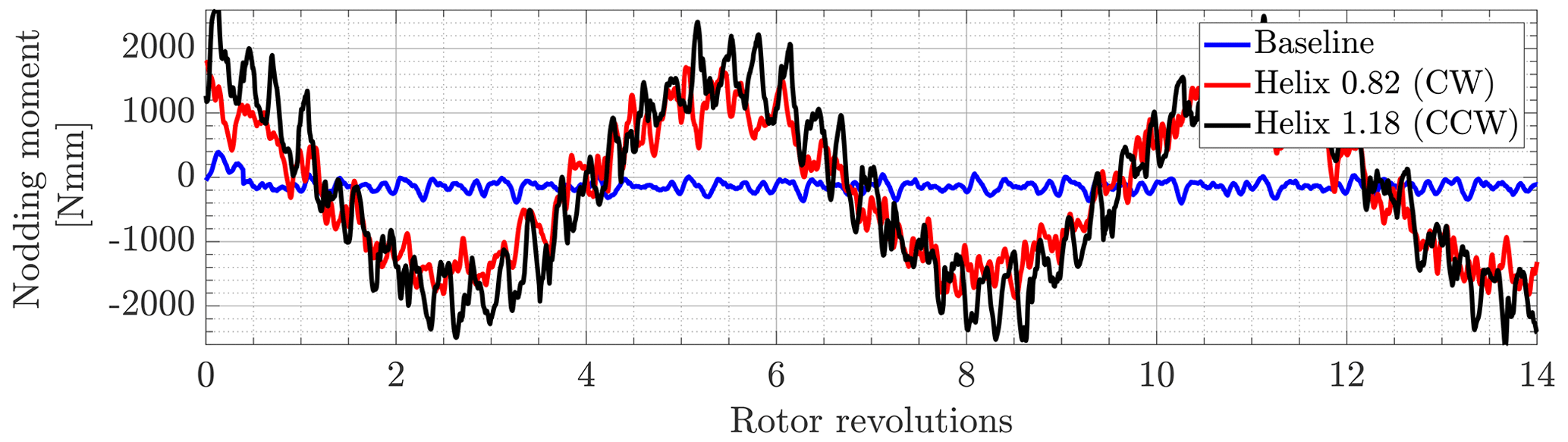
Figure 5 Fixed-frame nodding moment (time domain) for baseline (blue), Helix 0.82 (red), and Helix 1.18 (black).

4 Results

In the following section, the results of the experimental measurement campaign will be presented and discussed. Firstly, the results on turbines level will be analyzed to see how the turbine is influenced by applying the Helix technique and to identify how the turbine performance is affecting the wake and its recovery. Secondly, the results of the wake will be presented. Here, the section starts with a time-averaged analysis and is followed by results from a phase-locked investigation using the rotor azimuth position and the additional Helix frequency for phase locking.

4.1 Turbine data

The turbine data presented in this chapter were gathered by the sensors located on board the G1s, which are described in more detail in Sect. 3.

Figure 5 shows the fixed-frame nacelle nodding moment of the upstream turbine, corrected by the gravity-induced load. Specifically, the figure depicts the moment recorded during 14 rotor revolutions (equivalent to 1 s of measurement) for the baseline case, the Helix 0.82/CW case, and the Helix 1.18/CCW case. The yawing moment would show similar behavior, just offset by 90°, and would not reveal new insight. For this reason, it is not reported here. The graph confirms the expectation, e.g., that the implemented pitch actuation leads to the desired behavior of the nodding and yawing moments. The moment for the baseline case is indeed only fluctuating slightly due to mechanical vibrations and the not null turbulence intensity of the wind tunnel inflow. The nodding moment for the two Helix cases instead shows a very clear sinusoidal variation at the desired frequency, i.e., 2.5 Hz.

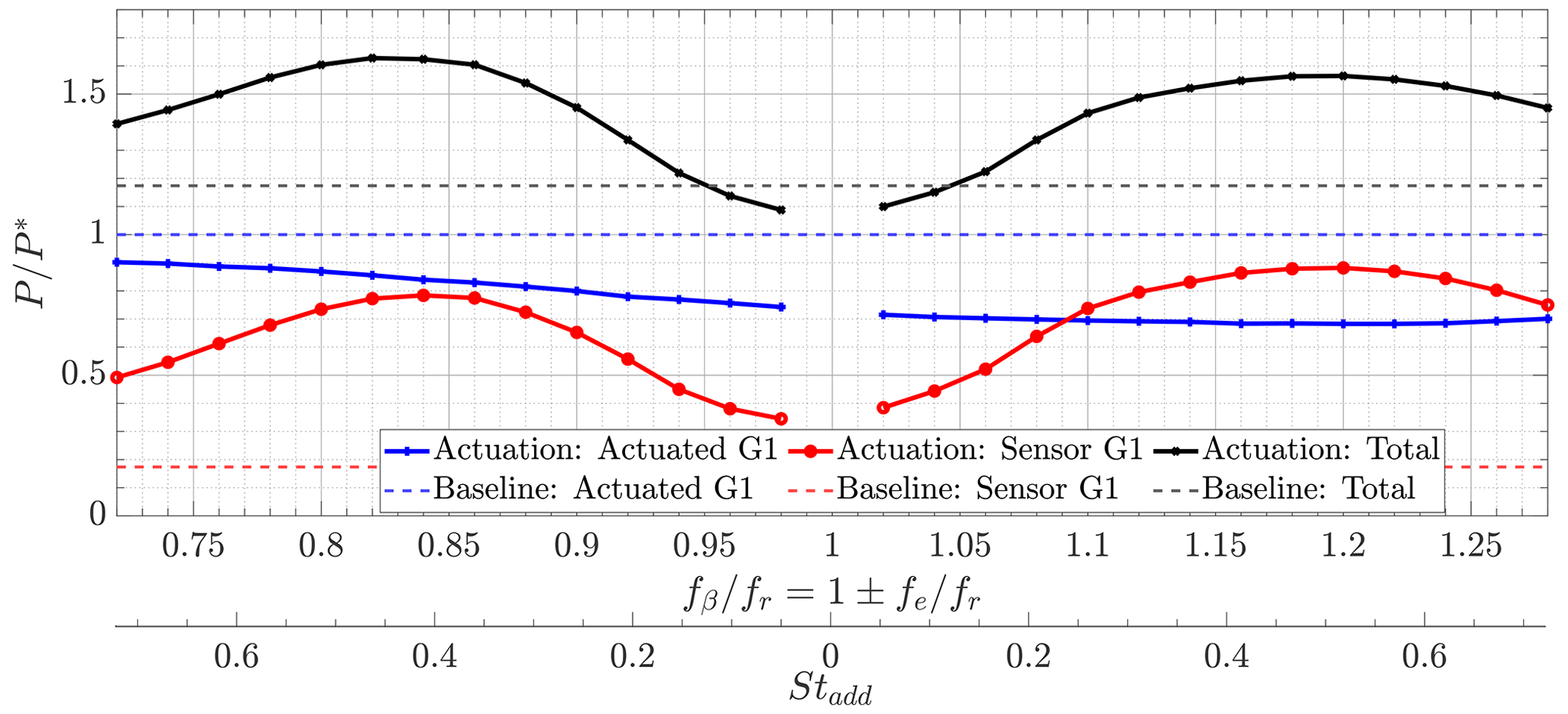
Figure 6 Extracted power of the upstream/actuated turbine, downstream/sensor turbine, and combined turbine array for changing pitch frequencies $f_{\mathit{\beta }}/f_{\mathrm{r}}=(\mathrm{0.72}:\mathrm{0.02}:\mathrm{1.28})$ compared to the baseline case without any actuation f_β=0 (dashed line).

This is confirmed by the Fourier transformation single-sided amplitude spectra of the nodding and yawing moments in the fixed-frame coordinate system. In addition to the peak at the rotational frequency f_r = 14 Hz, the Helix cases also experience a significant peak at the additional frequency f_e≈0.18f_r = 2.5 Hz, which is more than 1 order of magnitude bigger than the rotational frequency events.

The extracted powers of both wind turbines can be seen as an integral metric for the turbine performance. The summation of the two powers shows the overall performance of the whole setup. Figure 6 depicts the results of the power investigations by changing the actuation frequency of the first turbine in the range of $f_{\mathit{\beta }}/f_{\mathrm{r}}=(\mathrm{0.72}:\mathrm{0.02}:\mathrm{1.28})$. The extracted powers P are normalized by the power of the upstream/actuated turbine in the baseline scenario P^∗, where no actuation is present and the pitch is kept constant at $\mathit{\beta }={\mathit{\beta }}_{\mathrm{0}}\ne f\left(t\right)$.

In general, the extracted power of the actuated turbine decreases for all frequencies, since it is operated in a non-optimal operating point. With an increasing actuation frequency, this effect is also increasing. The decrease is particularly significant (around 30 %) for the highest actuation frequencies and is remarkably higher than the values (a few percent) noted in previous research works based on CFD (Frederik et al., 2020a) and aeroelastic (Taschner et al., 2023b) simulations. Whatever the reason for this difference may be – different performance of the G1 compared to that of a full-scale machine, wall blockage affected by the actuation frequency, physical effects not modeled in the simulation environments – further investigation is needed.

The behavior in terms of extracted power of the downstream/sensor turbine shows a remarkable trend. The curves are not perfectly mirrored along an axis in the 1 P frequency, but clearly, two distinct local maxima can be identified at $f_{\mathit{\beta }}/f_{\mathrm{r}}<\mathrm{1}$ and $f_{\mathit{\beta }}/f_{\mathrm{r}}>\mathrm{1}$. As already discussed in Frederik et al. (2020a), these two peaks are located at the identical additional excitation frequency of f_e=0.18f_r, referring to identical Strouhal numbers St_add≈0.47. Moreover, it can be seen that the trend of decreasing power with higher excitation does not apply to the downstream turbine, where the effect is the opposite, which is suggesting higher available power in the wake with a faster pitch excitation of the front turbine. When looking at the total power of the two-turbine setup, which is presented by the black line in Fig. 6, one can see that the opposite power behavior of the upstream and downstream turbines is almost evened out. The result is a nearly symmetrical behavior for clockwise and counterclockwise rotation. In the following, the wake investigations will focus on these two peaks. The corresponding scenarios are named according to the helical movement of the wake in either a clockwise (CW) $f_{\mathit{\beta }}/f_{\mathrm{r}}<\mathrm{1.0}$ or counterclockwise direction (CCW) $f_{\mathit{\beta }}/f_{\mathrm{r}}>\mathrm{1.0}$. The identified pitch frequencies are $(f_{\mathit{\beta }}/f_{\mathrm{r}}){|}_{\text{CW}}=\mathrm{0.82}$ and $(f_{\mathit{\beta }}/f_{\mathrm{r}}){|}_{\text{CCW}}=\mathrm{1.18}$, and the two cases are hereafter referred to as Helix 0.82 and Helix 1.18, respectively.

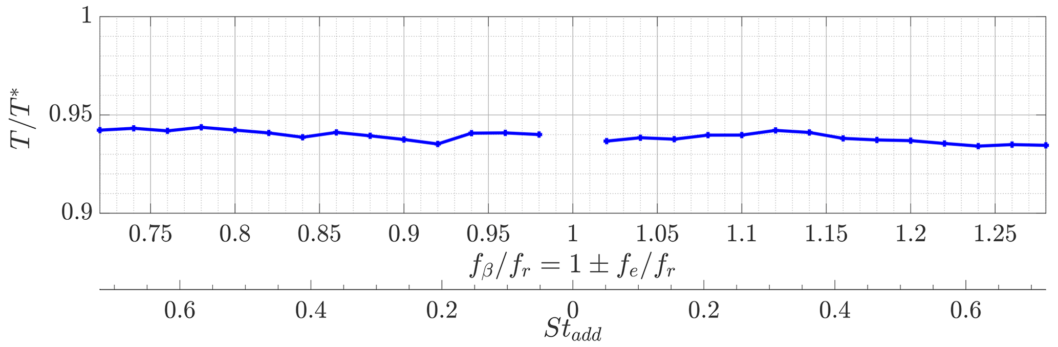
Figure 7 Thrust T of the upstream turbine for changing pitch frequencies $f_{\mathit{\beta }}/f_{\mathrm{r}}=(\mathrm{0.72}:\mathrm{0.02}:\mathrm{1.28})$, normalized with the thrust T^∗ of the baseline case.

Figure 7 shows the thrust T of the actuated upstream turbine, normalized by the thrust of the upstream/actuated turbine in the baseline scenario T^∗. The trend for T differs from the one of the normalized power of the upstream turbine in Fig. 6: the thrust is indeed reduced by the Helix but remains quite constant with increasing actuation frequencies (only a minor reduction is observed). Once again, the reason for the different trends observed for power and thrust requires further analysis.

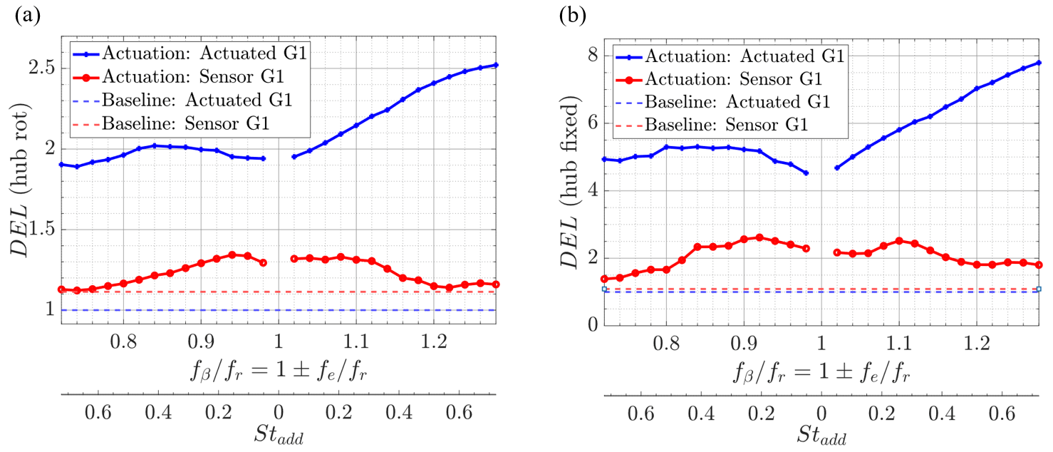
Figure 8 Normalized DELs of the upstream/actuated turbine and downstream/sensor turbine for (a) rotating hub and (b) fixed hub for changing pitch frequencies $f_{\mathit{\beta }}/f_{\mathrm{r}}=(\mathrm{0.72}:\mathrm{0.02}:\mathrm{1.28})$ compared to the baseline case without any actuation f_β=0 (dashed line).

The almost constant trend of the thrust would suggest a velocity deficit in the wake that does not depend on the actuation frequency. However, the available power for the downstream turbine has a higher peak for $f_{\mathit{\beta }}/f_{\mathrm{r}}>\mathrm{1.0}$ than f_βf_r<1.0. Consequently, the differences in power peaks of the sensor turbine for $f_{\mathit{\beta }}/f_{\mathrm{r}}\ne \mathrm{1.0}$ must come from mixing mechanisms in the wake, which might be caused by the opposite rotational direction of the additional wake rotation. Moreover, as seen in Fig. 7, the $P/P^{\ast }$ graph of the sensor turbine has two distinct peaks at almost identical Strouhal numbers for CW and CCW rotational direction. These two peaks are not present for the actuated upstream turbine, which is barely dependent on the Strouhal number. Additionally, it can be assumed that this effect is influenced by wake-mixing mechanisms and is not influenced by the performance of the upstream turbine.

In addition, the application of the IPC for the Helix control technique is without a doubt increasing the duty cycles of the pitch mechanism compared to the non-actuated baseline case, as the IPC control demands a constant operation of the pitch motors. Figure 8 reports the damage equivalent loads (DELs) at the rotating shaft (HubRotDEL; Fig. 8a) and at the nacelle (HubFixedDEL; Fig. 8b) for both G1s, which were computed as follows. First, load signals were filtered above 6 times the rotor frequency (6 × Rev) to remove high-frequency load components. Signal demodulation was then adopted for correcting the nacelle loads of their 1 × Rev harmonic component due to a slight inertial and aerodynamic imbalance of the rotor. Once the imbalance-induced spurious harmonic was removed, the loads were then projected back to the rotating frame to obtain corrected values of the rotating shaft loads. Moreover, DELs were obtained by projecting the corresponding two orthogonal bending moments on the direction associated with the maximum DEL. Furthermore, the figure depicts normalized DEL, obtained dividing the DELs by $\mathrm{1}/\mathrm{2}\mathit{\rho }\mathit{\pi }{R}^{\mathrm{3}}{V}_{\text{REWS}}^{\mathrm{2}}$. The depicted data, reported as a function of $f_{\mathit{\beta }}/f_{\mathrm{r}}=(\mathrm{0.72}:\mathrm{0.02}:\mathrm{1.28})$, highlight that the loads are increasing, for both the upstream and downstream turbines and for both load channels, if the front turbine implements the Helix. For the upstream turbine, the loads increase with ascending actuation frequency.

For the sensor turbine, the loads do not show a dependency on the actuation frequency but towards the Strouhal number. They almost show an identical shape for a CW and a CCW actuation. For lower Strouhal numbers the loads are larger. At the optimal Strouhal number (St_add≈0.47) they are almost at the level of the reference case. The dependency on the Strouhal number is similar to the behavior of the available power behind the actuated turbine. However, for the loads investigation, there are no distinct peaks comparable to the ones observed for $P/P^{\ast }$ of the downstream turbine.

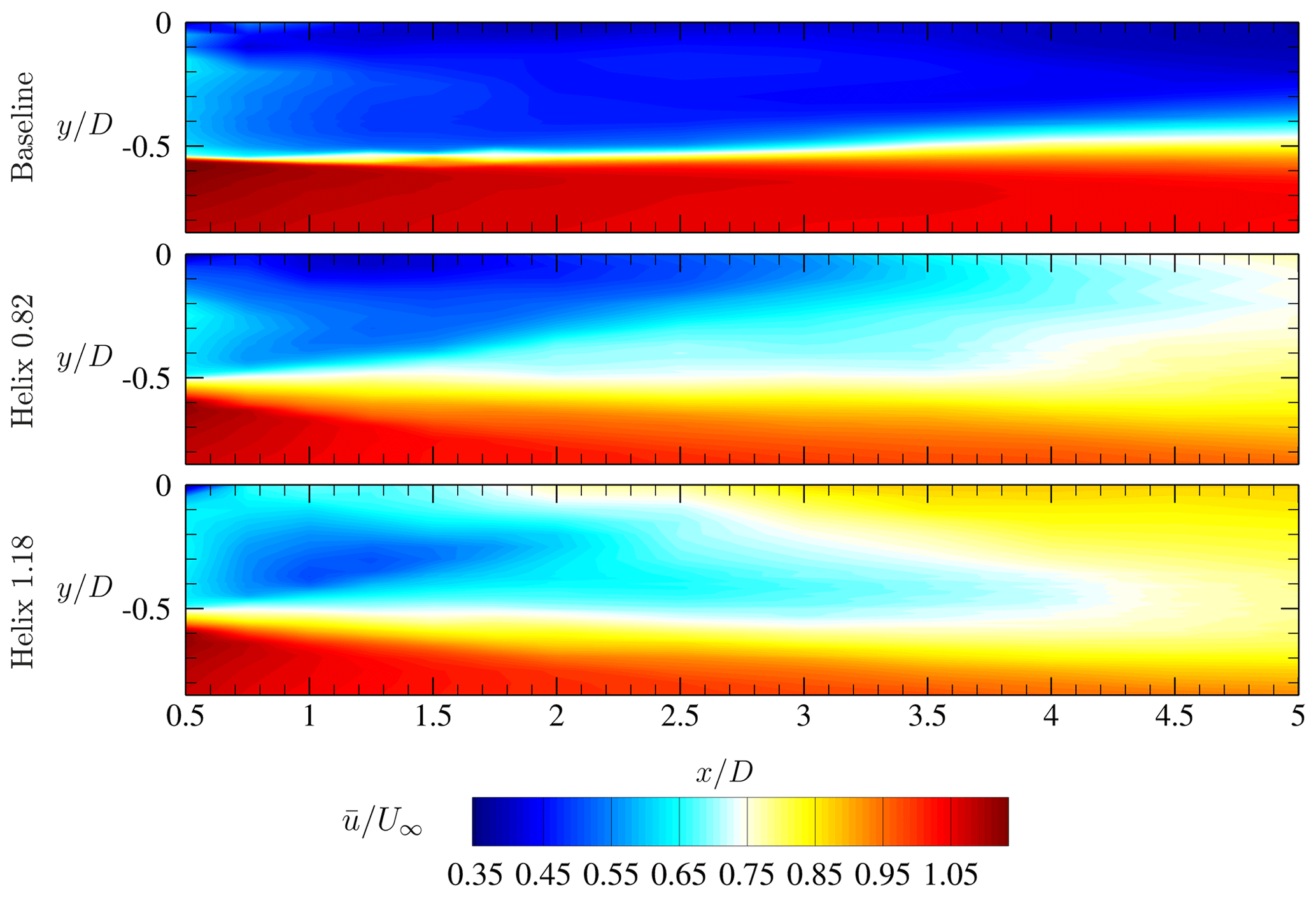
Figure 9 Contour plot of the normalized time-averaged streamwise velocity component $\stackrel{\mathrm{‾}}{u}/U_{\mathrm{\infty }}$ for the baseline case and the two actuated cases Helix 0.82 and Helix 1.18.

The design of most wind turbine components, such as the tower, blades, or main shaft, is mainly driven by (1) the need to withstand the expected fatigue loads over their entire lifespan and (2) the need to withstand the ultimate loads that might act on the wind turbine even only once in its lifetime. To what extent the design is driven by the fatigue or ultimate loads depends on the machine itself and the component under consideration. The impact of the increased fatigue loads induced by the Helix should, therefore, be assessed specifically for each machine on which it is to be implemented and can be more or less significant depending on the role played by fatigue in the design process.

To summarize, a sinusoidal individual pitch actuation causes a sinusoidal variation in the nodding and yawing moment with strong energy content at the additional rotation frequency. The hub loads for the actuated and sensor turbines are increasing in the case the Helix control is applied, whereas the actuated turbine shows a larger load increase than the sensor turbine. If the turbine is controlled with the Helix technique, the power decreases with ascending additional actuation frequency. However, the power readings of the sensor turbine show very strong gains of the available power behind the actuated turbine with two distinct local maxima at almost identical Strouhal numbers St_add. These cases with the maximum extracted power ($(f_{\mathit{\beta }}/f_{\mathrm{r}}){|}_{\text{CW}}=\mathrm{0.82}$ and $(f_{\mathit{\beta }}/f_{\mathrm{r}}){|}_{\text{CCW}}=\mathrm{1.18}$ at St_add≈0.47) are chosen for the wake investigations in the next section and are compared to the wake of the reference case.

4.2 Wake data

The following section covers the main results of the measurements conducted with the FRAP in the wind turbine wake for the reference case and the two actuated cases $(f_{\mathit{\beta }}/f_{\mathrm{r}}){|}_{\text{CW}}=\mathrm{0.82}$ and $(f_{\mathit{\beta }}/f_{\mathrm{r}}){|}_{\text{CCW}}=\mathrm{1.18}$ at St_add≈0.47. Hence, the downstream turbine is removed from the W/T (second stage setup), and the probe is traversed according to the measurement grid described in Sect. 3. All measurements are conducted at hub height $z/D=\mathrm{0}$.

4.2.1 Time-averaged wake flow

Firstly, the time-averaged flow field will be presented and discussed. In Fig. 9, contour plots of the normalized time-averaged streamwise velocity component $\stackrel{\mathrm{‾}}{u}/U_{\mathrm{\infty }}$ for the baseline, Helix 0.82, and Helix 1.18 cases are shown. In accordance with the findings in the extracted power observations, the wake velocity has recovered earlier for the actuated cases. This effect is already noticeable at a short distance behind the rotor where a weaker wake border is present for the actuated scenarios and is getting more pronounced at larger downstream distances. However, small differences in the wake shape can be seen between the two actuated cases. The Helix 1.18 streamwise velocities at lateral positions close to the centerline recover earlier and show higher wake velocities. While the baseline case wake provides a sharper border in the tip vortex region, it starts to show entrainment at downstream distances around $x/D=\mathrm{2}$. Nevertheless, a clear separation between the low- and high-energy flow fields is still present at $x/D=\mathrm{5}$. In the actuated cases, already at the most upstream measurement location $x/D=\mathrm{0.5}$, the tip vortex region is quite broad and no distinct sharp wake border can be identified. Consequently, the wake is not shielded from the outer, high-energy flow, and entrainment of energy starts much earlier as in the baseline case. This leads to a faster recovery, which can be confirmed by the higher velocities in the wake region. Both actuated cases show streamwise velocities above $\stackrel{\mathrm{‾}}{u}/U_{\mathrm{\infty }}>\mathrm{0.7}$ at the former location of the downstream turbine (sensor G1 in first stage setup) at $x/D=\mathrm{5.0}$, confirming the two distinct power peaks observed in Fig. 6.

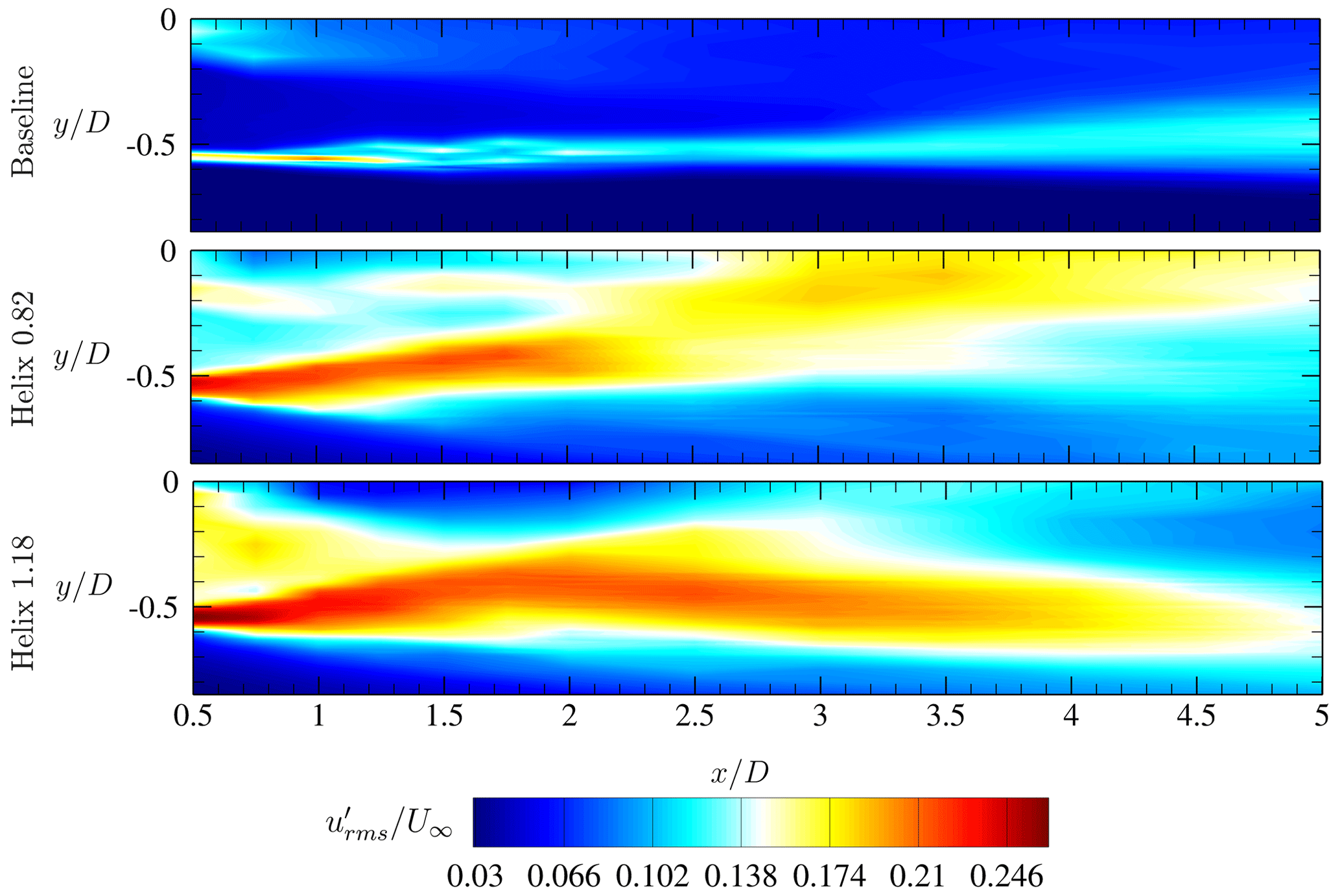
Figure 10 Contour plot of the normalized time-averaged rms values of the streamwise fluctuations $u_{\text{rms}}^{\prime }/U_{\mathrm{\infty }}$ for the baseline case and the two actuated cases Helix 0.82 and Helix 1.18.

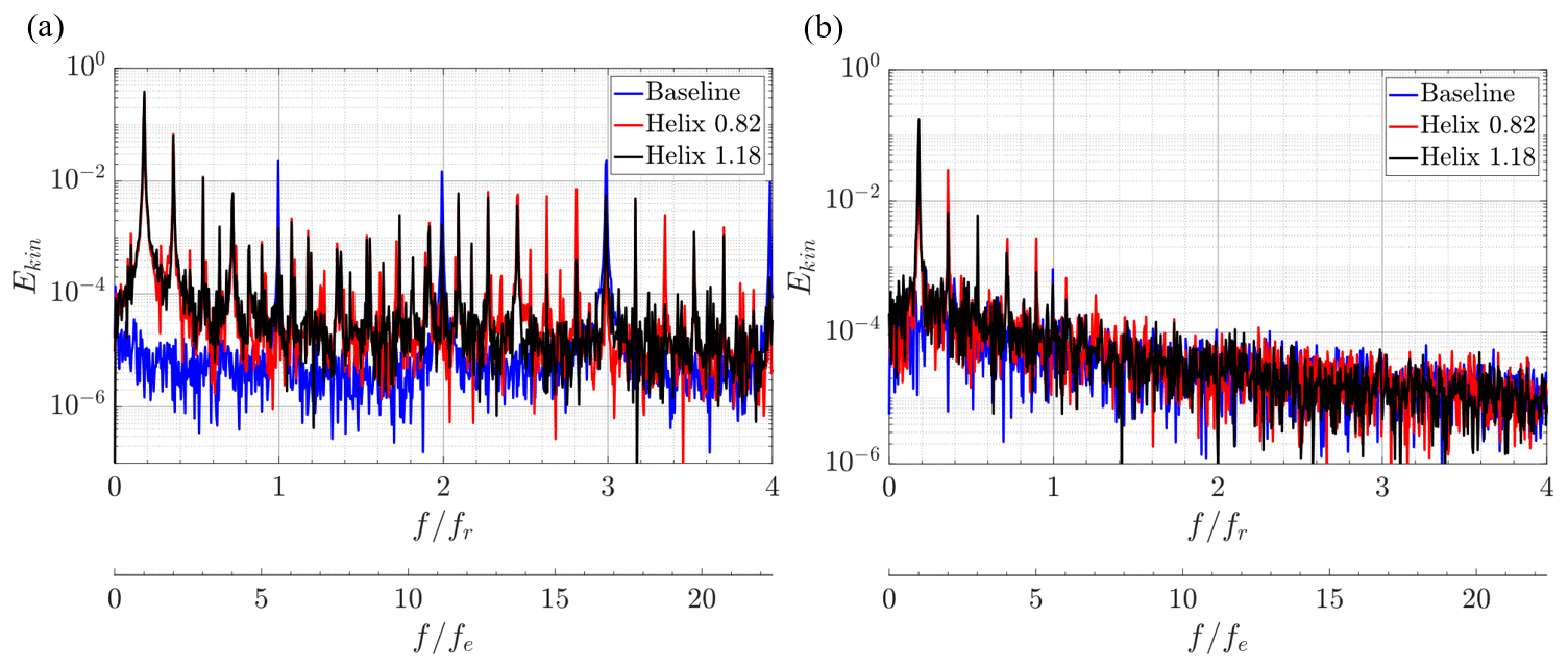
Figure 11 Kinetic energy spectra E_kin at various measurement locations in the turbine wake at $x/D=\mathrm{0.5}$ and (a) $y/D=-\mathrm{0.55}$ and (b) $y/D=-\mathrm{0.15}$.

In order to determine the instability mechanisms that are dominant and the location where they occur, Fig. 10 shows contour plots of the normalized time-averaged rms values of the streamwise fluctuations $u_{\text{rms}}^{\prime }/U_{\mathrm{\infty }}$ for the three cases. For the baseline case, the highest fluctuations occur in the region where the tip vortices move downstream and separate the wake. Between $x/D=(\mathrm{1.0},\mathrm{2.0})$, the onset of a mixing process can be detected, and hence, leapfrogging is expected. In contrast to the flow patterns in the baseline case, in the actuated cases, increased fluctuation contents are already detectable in the wake. These fluctuations enable an entrainment of the energy-containing flow from outside into the wake. Thereby, mixing is promoted, and an earlier recovery of the wake is visible.

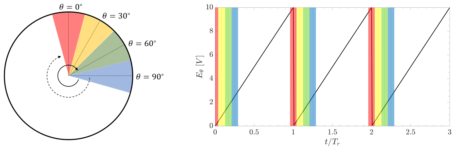
Figure 12 Phase-locking principle visualized by the rotational location of the blade θ and the acquired analog output signal voltage E_θ.

As a next step, in order to discover the governing mechanisms in the actuated cases, kinetic energy spectra are calculated for various locations in the wake of the turbine. Figure 11 shows the spectra at two locations: $P\mathrm{1}=(x/D,y/D)=(\mathrm{0.5},-\mathrm{0.55})$ and $P\mathrm{2}=(\mathrm{0.5},-\mathrm{0.15})$. As expected, the baseline spectra solely experience peaks at the rotational frequency f_r = 14 Hz and its higher harmonics. In the more inward locations inside the wake at $y/D=-\mathrm{0.15}$, these peaks are barely detectable. Looking at the spectra of the actuated cases, the system is governed by multiple higher harmonic peaks, based on the first harmonic of the additional excitation frequency f_e = 2.5 Hz. As already seen in the turbine hub moments, the system is governed by the excitation frequency f_e instead of the rotational frequency f_r as seen in the baseline flow. Especially at the low bandwidth, additional energy is added for the actuated cases. Together with the velocity plots already shown in Fig. 9, it can be concluded that low-bandwidth content due to the additional out-of-sync actuation is introduced in the entire wake $|y/D|<\mathrm{0.5}$, leading to earlier entrainment and faster wake recovery.

In addition, transient flow data are analyzed with respect to phase-locked information.

4.2.2 Wake flow analysis: results phase-locked with the rotor azimuthal position

In this section, a more detailed analysis of the transient wind turbine wake is conducted using phase-locked postprocessed data obtained from the FRAP measurements and the azimuthal blade position signal. Figure 12 schematically depicts the principle of the phase-locking process. Each rotation with a rotational period T_r is equally divided into N segments. In this schematic figure, the full rotation is exemplarily divided into N=12 segments $\mathrm{\Delta }\mathit{\theta }=\mathrm{360}\mathit{°}/N=\mathrm{30}\mathit{°}$. All data points inside a segment and in corresponding segments of the same phase (same color) in the upcoming rotational periods are gathered and averaged to a single value, i.e., the phase-locked value for this segment. In the wake measurements, the azimuthal position θ is processed in the form of a saw tooth analog signal, where E_θ = 0 V and E_θ = 10 V correspond to θ = 0° and θ = 360°, respectively. So the FRAP measurements can be conducted without any further trigger mechanism and are fully synchronized in the postprocessing steps via the phase-locking procedure shown.

In the following analysis, one rotational period was divided into 120 segments. Thus, each phase-locked value maps data of a segment of Δθ = 3°.

It has to be noted that the results present the phase-locking with the rotational period T_r. Since the actuation of the blade pitch is slightly out of sync, the results cannot fully show a transient behavior as it really occurs at the blade. Only a phase-locked-averaged investigation is possible. For the baseline case, since no blade pitch actuation is active, the phase-locked results represent a realistic visualization of the flow over one rotor revolution.

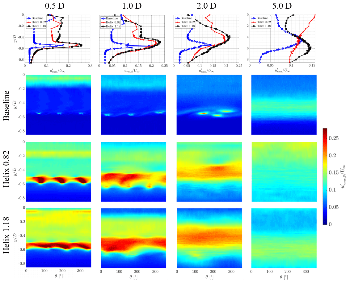
Figure 13 Normalized phase-locked rms values of the streamwise fluctuations $u_{\text{rms},\mathit{\theta }}^{\prime }/U_{\mathrm{\infty }}$ at multiple downstream positions $x/D=\mathit{\{}\mathrm{0.5},\mathrm{1.0},\mathrm{2.0},\mathrm{5.0}\mathit{\}}$.

Figure 13 represents the basis for the discussion of the rotor azimuth phase-averaged results of the turbine wake. Data were gathered at four downstream line locations $x/D=\mathit{\{}\mathrm{0.5},\mathrm{1.0},\mathrm{2.0},\mathrm{5.0}\mathit{\}}$ and are shown for the phase-averaged rotation θ = 0–360°. Furthermore, in order to link to the time-averaged results from Sect. 4.2.1, time-averaged line plots are also shown in the figure. For the sake of consistency, the axes are switched to have a matching y axis with the phase-locked contour plots. The phase-averaged results for $u_{\text{rms},\mathit{\theta }}^{\prime }/U_{\mathrm{\infty }}$ will be discussed in the following, as they contain the necessary information to explain the mechanisms in the wake. The index ()_θ indicates the phase-averaged property.

Closely behind the rotor, the baseline case experiences three distinct, separated peaks at $y/D\approx -\mathrm{0.55}$ due to the three tip vortices per revolution. Furthermore, the fluctuation level resulting from the root vortex system near the centerline $y/D\approx -\mathrm{0.05}$ is increased, and higher fluctuations are detected. In the baseline case, between $x/D=(\mathrm{1.0},\mathrm{2.0})$, the leapfrogging instability mechanism occurs, which is shown by a representation of the normalized phase-locked rms values of the streamwise fluctuations $u_{\text{rms},\mathit{\theta }}^{\prime }/U_{\mathrm{\infty }}$. At $x/D=\mathrm{1.0}$, a clear separation of three distinct vortices per revolution can still be detected. The phase difference between the occurrence of the vortices is still approximately Δθ=120°, as expected for a three-bladed turbine. However, a first inward movement is seen, and hence, the instability and interaction between the helical vortices are introduced. In more downstream positions, the roll-up process of multiple vortices starts and results in an almost complete merging of the three vortices to a single structure at $x/D=\mathrm{2.0}$. At $x/D=\mathrm{5.0}$ the individual vortices merged completely into a coherent structure.

When discussing the velocity fluctuations in the line plots in the top row of Fig. 13, higher levels of perturbations can be seen throughout all lateral positions $y/D$ for the Helix cases for all investigated downstream distances $x/D$. Thus, more mixing is already present in the very near wake of the actuated cases. It is therefore assumed that no conventional instability mechanism, like the leapfrogging mechanism, can be accounted for in the wake recovery. This observation is enhanced by the contour plots for the actuated cases. At the nearest downstream line location at $x/D=\mathrm{0.5}$, a band of high fluctuations with separated peaks (Δθ≈ 120°) is detected for both Helix cases. These structures do not show coherent vortex filaments as in the baseline case. They are already merged at the downstream location $x/D=\mathrm{1.0}$. At $x/D=\mathrm{5.0}$ the flow for the actuated cases is almost uniform along the phase-locked time. Compared to the Helix 0.82 case, the Helix 1.18 case shows a more uniform and higher fluctuation level throughout the full revolution. As can be seen in the more downstream contour figure, the additional fluctuations provoke an earlier mixing and entrainment of higher-velocity flow from the outer area leading to a more uniform fluctuation level at $x/D=\mathrm{5.0}$.

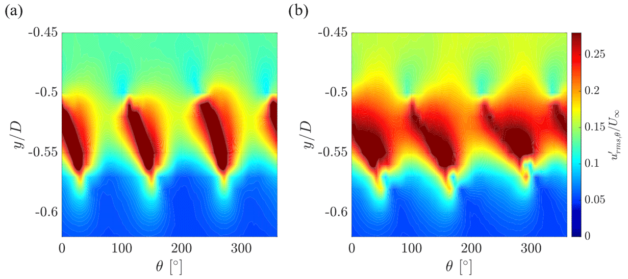
Figure 14 Normalized phase-locked rms values of the streamwise fluctuations $u_{\text{rms},\mathit{\theta }}^{\prime }/U_{\mathrm{\infty }}$ at a downstream position of $x/D=\mathrm{0.35}$ for (a) Helix 0.82 and (b) Helix 1.18.

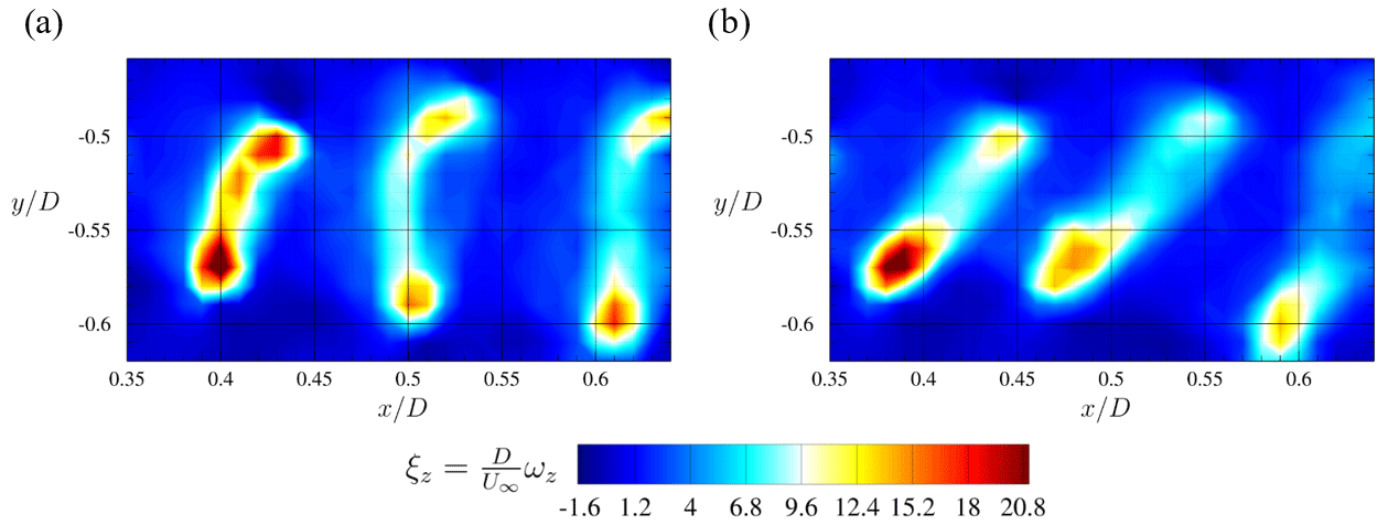
Figure 15 Normalized phase-locked vorticity in z direction ξ_z at azimuthal position θ= 90° for (a) Helix 0.82 and (b) Helix 1.18. Video link: https://youtu.be/ta3KwE5yuSQ.

In order to understand the flow physics for the actuated cases better and to explain the band of high fluctuations directly behind the rotor, further refinement at locations closer to the turbine is performed. A refined measurement grid in the region between $y/D=(-\mathrm{0.45},-\mathrm{0.62})$ and $x/D=(\mathrm{0.35},\mathrm{0.64})$ (shown in red in Fig. 2 c) for both actuated cases is defined, and additional measurements are conducted. The spatial distance between the points is fixed to $\mathrm{\Delta }(y/D)=\mathrm{\Delta }(x/D)=\mathrm{0.01}$ in each direction. The contour plots in Fig. 14 show the normalized phase-locked rms values of the streamwise fluctuations $u_{\text{rms},\mathit{\theta }}^{\prime }/U_{\mathrm{\infty }}$ over one rotation at the closest distance $x/D=\mathrm{0.35}$ for both actuation cases. As already mentioned before, both cases experience high fluctuation levels of around $u_{\text{rms},\mathit{\theta }}^{\prime }/U_{\mathrm{\infty }}\approx \mathrm{0.25}$ between lateral locations $y/D=(-\mathrm{0.5},-\mathrm{0.57})$. However, the Helix 1.18 contours are more smeary, and hence, a more constant input of fluctuation is seen over one rotor revolution. As already mentioned, this representation does not show realistic vortex shedding since the actuation is out of sync with the rotational frequency, which is the basis for the phase-locking procedure. The phenomena shown here describe multiple flow situations that occur throughout the actuation time.

To get a more thorough view of the whole area of the refined grid, phase-locked contour plots of the entire refined measurement x–y plane are shown in Fig. 15. In this figure, the normalized phase-locked vorticity in the z direction (out of plane) ξ_z is shown for the azimuth blade position θ = 90°. The figures are screenshots of a video consisting of multiple phase-locked positions corresponding to azimuth blade positions θ = 0–360°. The videos for the two Helix cases can be found via the following link: https://youtu.be/ta3KwE5yuSQ. The normalized vorticity in z direction is calculated as follows:

$$\begin{array}{}\text{(2)}& {\mathit{\xi }}_z={\displaystyle \frac{D}{U_{\mathrm{\infty }}}}{\mathit{\omega }}_z={\displaystyle \frac{D}{U_{\mathrm{\infty }}}}\left({\displaystyle \frac{\partial v}{\partial x}}-{\displaystyle \frac{\partial u}{\partial y}}\right).\end{array}$$

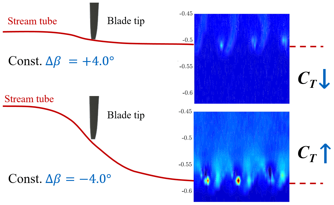
Figure 16 Normalized phase-locked rms values of the streamwise fluctuations $u_{\text{rms},\mathit{\theta }}^{\prime }/U_{\mathrm{\infty }}$ for fixed pitch $\mathrm{\Delta }\mathit{\beta }=-\mathrm{4}\mathit{°}$ and Δβ=4° at a downstream position of $x/D=\mathrm{0.35}$.

Once again, both actuated cases are directly compared in the figure. Here, vortex-sheet-shaped elongated structures travel downstream and broaden. Nevertheless, since solely phase-locked results are shown, which were locked with the rotational frequency f_r and not with the additional rotational frequency f_e, the “vortex sheets” visualize an averaged representation of the flow structures traveling downstream. For the Helix 0.82 case, the two vortices at the extreme $y/D$ positions move downstream with an almost identical speed. A C-shaped lateral elongated structure corresponding to the sinusoidal vortex shedding with different vortex strengths forms. In contrast to that, the Helix 1.18 case shows an additional delay in the shedding of the two extreme positions. A diagonal-shaped structure travels downstream in the phase-locked flow field.

To understand the elongated vortex structures in Fig. 15 better, two additional constant-pitch experiments are conducted. Within these measurements, the additional blade pitch is changed to a constant value matching either the minimum or the maximum of the dynamic blade pitch motion of the actuated cases $\mathrm{\Delta }\mathit{\beta }=\text{ const. }=\pm \mathrm{4}\mathit{°}$. Figure 16 shows the vortex shedding (visualized by $u_{\text{rms},\mathit{\theta }}^{\prime }/U_{\mathrm{\infty }}$) over one rotor revolution for the extreme fixed-pitch cases together with a sketch of the stream tube. For the Δβ = −4° case, blade loading and consequently C_T are increasing. Thus, a stronger vortex forms at the blade tip. With an increased C_T, the stream tube is expanding, leading to the tip vortex being shed rather outside at around $y/D=-\mathrm{0.57}$. The opposite happens for the Δβ = +4° case, where the high pitch angle leads to an unloaded turbine blade with a decreased C_T. Consequently, weaker tip vortices form and the wake stream tube does not widen up as for lower blade pitch angles and travels downstream at a more inward position of around $y/D=-\mathrm{0.50}$. The lateral position of the detectable vortices for the fixed-pitch cases matches the maximum values measured for the dynamically pitched Helix cases in Fig. 14 and explains the elongated shape of the tip vortices.

To get the full view of the transient flow behavior in the wake of the dynamically actuated wind turbine, further analysis can be conducted. Instead of phase-locking the data with the rotor azimuth as presented in this chapter, the additional excitation frequency f_e is used for phase-locking to see and understand what is happening with the wake flow during one additional rotation which is created by the Helix control.

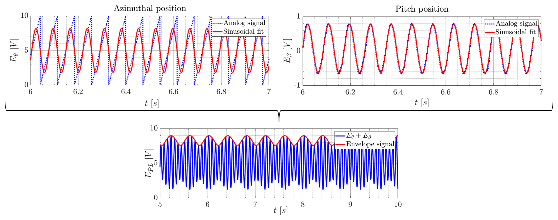
Figure 17 Schematic visualization of the process of extracting the envelope/beat frequency from the blade azimuthal and pitch position for phase-locking with the additional frequency.

4.2.3 Wake flow analysis: results phase-locked with the additional excitation frequency

In the following, phase-locked results are presented which use the additional excitation frequency f_e = 2.5 Hz as the phase-locking frequency. Since the measured data solely consist of the azimuth and the blade 1 pitch positions, the additional frequency signal has to be extracted from these signals at first. This is done by taking the envelope/beat frequency of the superposition of the two acquired signals. The output of this preprocessing step is a sinusoidal signal with f_e = 2.5 Hz that is used in the following to phase-lock the measured FRAP data. The process of extracting the envelope/beat frequency from the blade azimuth and pitch position is visualized in Fig. 17. After extracting the time series for the beat frequency for each individual measurement point, the measured FRAP data are phase-averaged with the beat frequency. Readings of all measurement points can thereby be correlated.

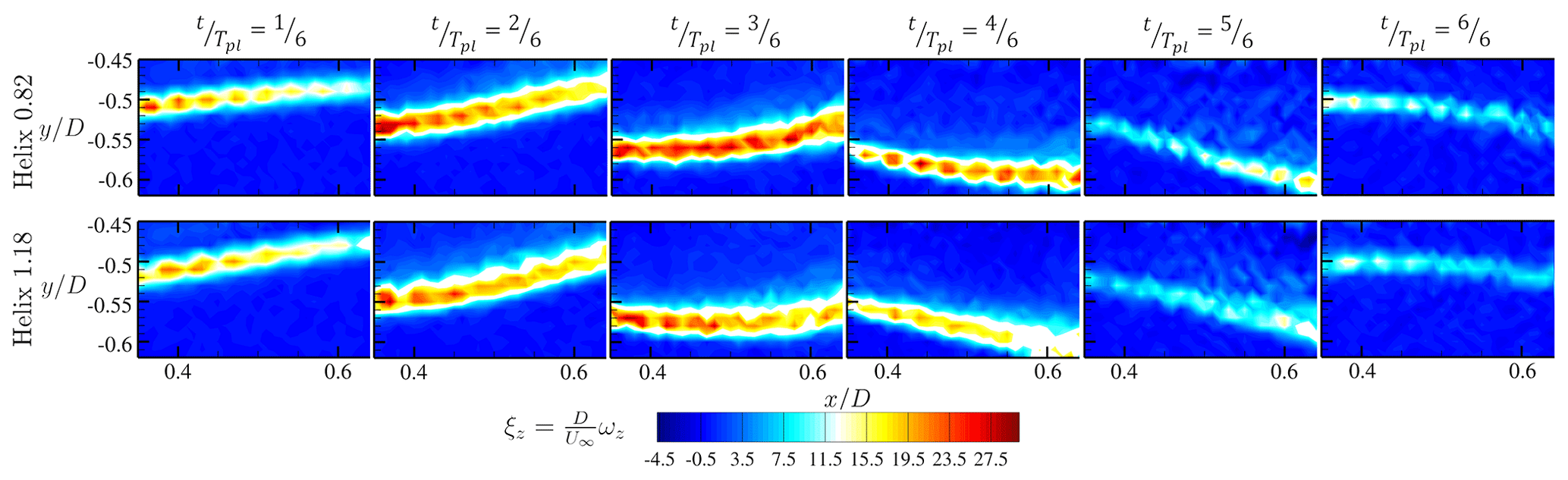
Figure 18 Normalized phase-locked vorticity in z direction ξ_z taken from the 12 s video for one additional rotation at the time steps $t/T_{\text{pl}}=\mathrm{1}/\mathrm{6}$, $t/T_{\text{pl}}=\mathrm{2}/\mathrm{6}$, $t/T_{\text{pl}}=\mathrm{3}/\mathrm{6}$, $t/T_{\text{pl}}=\mathrm{4}/\mathrm{6}$, $t/T_{\text{pl}}=\mathrm{5}/\mathrm{6}$, and $t/T_{\text{pl}}=\mathrm{6}/\mathrm{6}$ for Helix 0.82 (top) and Helix 1.18 (bottom). Video link: https://youtu.be/0x432E6h-7E.

In Fig. 18, the results of the phase-locking process with the additional frequency are compared for both actuated cases (Helix 0.82 top and Helix 1.18 bottom). The contour plots show the normalized phase-locked vorticity in the z direction (out of plane) ξ_z, which is calculated according to Eq. (2). In this way, the results can be compared to the ones from Fig. 15, which are representative of the phase-locking analysis with the azimuth position. An analysis of the streamwise fluctuations $u_{\text{rms}}^{\prime }/U_{\mathrm{\infty }}$ phase-locked with the additional frequency f_e resulted in similar plots that showed the same meandering motion and are for this reason not presented here. The figures show snapshots of multiple phase-locked positions for one complete phase-locking period T_pl. The six contour plots are taken with time steps of $\mathrm{\Delta }t=\mathrm{1}/\mathrm{6}\cdot T_{\text{pl}}$. The videos for the two Helix cases can be found via the following link: https://youtu.be/0x432E6h-7E.

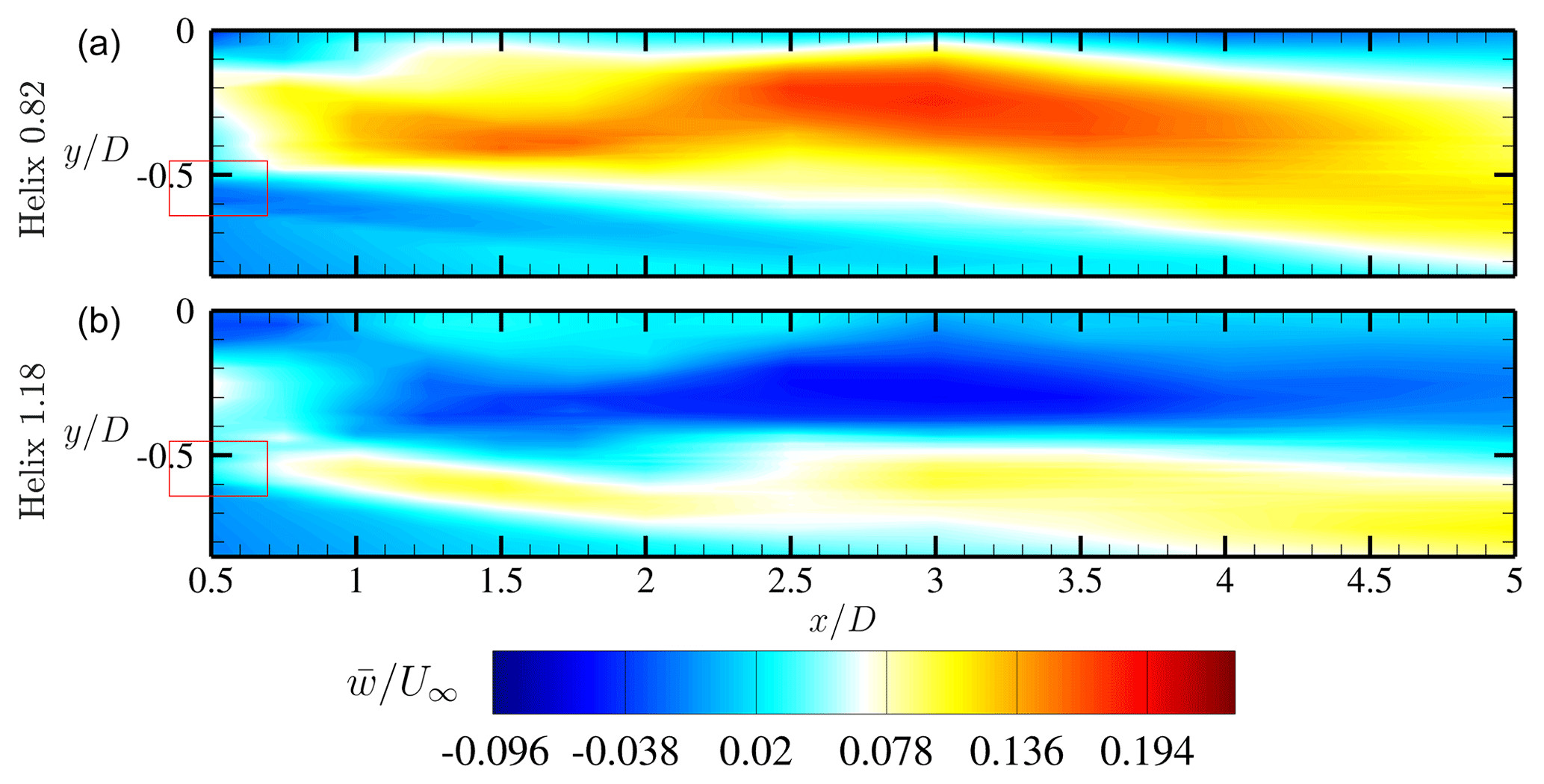
Figure 19 Contour of flow field for normalized average velocity in the out-of-plane component $\stackrel{\mathrm{‾}}{w}/U_{\mathrm{\infty }}$ for the two actuated cases Helix 0.82 (a) and Helix 1.18 (b). The red square defines the plane of the refined tip vortex analysis.

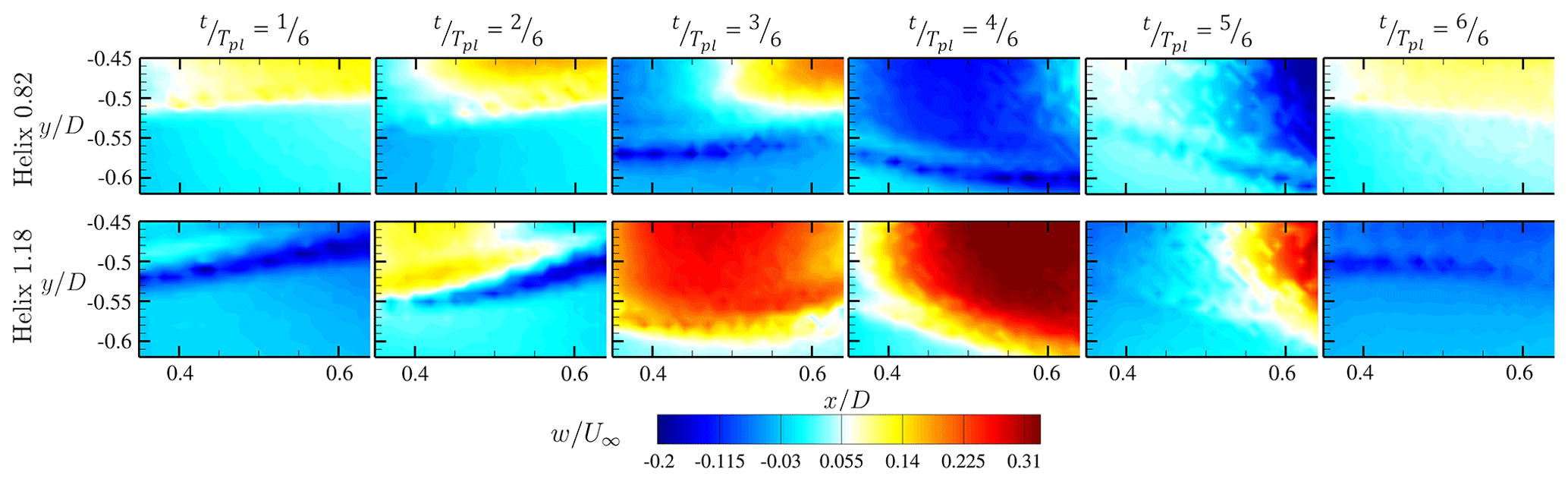
Figure 20 Normalized phase-locked velocity component $w/U_{\mathrm{\infty }}$ in z direction ξ_z taken from the 12 s video for one additional rotation at the time steps $t/T_{\text{pl}}=\mathrm{1}/\mathrm{6}$, $t/T_{\text{pl}}=\mathrm{2}/\mathrm{6}$, $t/T_{\text{pl}}=\mathrm{3}/\mathrm{6}$, $t/T_{\text{pl}}=\mathrm{4}/\mathrm{6}$, $t/T_{\text{pl}}=\mathrm{5}/\mathrm{6}$, and $t/T_{\text{pl}}=\mathrm{6}/\mathrm{6}$ for Helix 0.82 (top) and Helix 1.18 (bottom). Video link: https://youtu.be/KH06Y7n5_gA.

When analyzing the results in Fig. 18, it is clearly visible that different flow structures can be observed to be dependent on the locking frequency. Due to the rather long phase-locking period applied in this section ($T_{\text{pl}}=\mathrm{1}/f_{\mathrm{e}}$), the contours do not show the typical shedding of the three vortices but rather a vortex path which shows the shedding locations of multiple blade tip vortices over time. During one revolution of the additional rotational component, the tip vortex at $x/D=\mathrm{0.35}$ starts at $y/D\approx -\mathrm{0.50}$ at $t=\mathrm{1}/\mathrm{6}\cdot T_{\text{pl}}$ and travels laterally outwards until $y/D\approx -\mathrm{0.57}$ at $t=\mathrm{3}/\mathrm{6}\cdot T_{\text{pl}}$, from where it moves back towards the wake center. Furthermore, at this movement, a weakening of the magnitude can be observed. Looking at the farthest downstream location of the measurement plane at $x/D=\mathrm{0.64}$, the vortex path is slightly lagging behind in time and moreover shows an even wider lateral expansion than at $x/D=\mathrm{0.35}$. Hence, this indicates an increasing mixing effect at more downstream positions. The observations taken from the phase-locked data show that the tip vortex path performs a meandering movement. Moreover, the tip vortices for the two Helix cases look quite similar, both in shape and in magnitude. These observations confirm the conclusions drawn from the vorticity magnitudes in the results phase-locked with the rotor azimuth position in Fig. 15. These are backed by the findings of the C_T graph and the lateral tip vortex position changes for the constant extreme pitch angles $\mathrm{\Delta }\mathit{\beta }=\text{ const. }=\pm \mathrm{4}\mathit{°}$. Due to the changing blade pitch β and thus a varying C_T, the vortex shedding is traveling back and forth in a lateral direction over time. Furthermore, the results confirm that a traditional vortex interaction mechanism through leapfrogging as seen in the reference case is not present in the Helix actuation. Consequently, the meandering of the vortex in the blade tip region is expected to be the main driver for the increased wake mixing for the Helix technique.

4.2.4 Out-of-plane velocity

This last section of the results is intended to explain the differences between the Helix 0.82 and Helix 1.18 cases. For this, an analysis of the rotational velocity component is conducted. In the presented case, in which the velocity is mapped on an x–y plane, the velocity component w in the out-of-plane z direction represents the rotational direction of the wake. As already mentioned in the explanation of the control technique in Sect. 2, the actuation of the out-of-sync blade pitch provokes an additional clockwise or counterclockwise rotation of the wake. Figure 19 shows contours of the investigated flow field of the normalized averaged velocity in the out-of-plane component $\stackrel{\mathrm{‾}}{w}/U_{\mathrm{\infty }}$. It can be seen that the two Helix cases $\stackrel{\mathrm{‾}}{w}/U_{\mathrm{\infty }}$ are in significant contrast to each other. For the Helix 0.82 case, the velocity $\stackrel{\mathrm{‾}}{w}/U_{\mathrm{\infty }}$ in the inner part of the wake $|y/D|<\mathrm{0.5}$ is positive, whereas the outer part $|y/D|>\mathrm{0.5}$ is slightly negative, pointing in the same direction as the additional rotation of the 0.82 Helix excitation. For this case the w velocity magnitude is rather low as the additional rotational component is opposite to the wake rotation. The Helix 1.18 case, in contrast, shows a contrary behavior. The inner part shows slightly negative velocities, whereas the outer part is rotating in a CCW rotation. Here the additional rotational component of the Helix is added to the wake rotation. Hence, $\stackrel{\mathrm{‾}}{w}/U_{\mathrm{\infty }}$ has a larger magnitude compared to the Helix 0.82 case.

The formation of this contrary sheared flow can be observed when looking into the refined tip vortex region, which is presented in Fig. 20 showing contours of the normalized velocity component $w/U_{\mathrm{\infty }}$, phase-locked with the additional frequency taken from a 12 s video for one additional rotation at six time steps from $t/T_{\text{pl}}=\mathrm{1}/\mathrm{6}$ to $t/T_{\text{pl}}=\mathrm{6}/\mathrm{6}$. For the Helix 0.82 case presented on top, the meandering shear border is located towards the center of the wake. The phase-locked velocity $\stackrel{\mathrm{‾}}{w}/U_{\mathrm{\infty }}$ is positive in the inner section at the beginning of the period T_pl and changes its sign when meandering outwards $t/T_{\text{pl}}>\mathrm{2}/\mathrm{6}$. The opposite can be observed for the Helix 1.18 case, where a change from negative to positive velocities is observed after the wake is meandering from the center $t/T_{\text{pl}}\le \mathrm{2}/\mathrm{6}$ outward $t/T_{\text{pl}}\ge \mathrm{3}/\mathrm{6}$. The strongest magnitudes can be observed when the meandering border reaches the utmost point at time steps $t/T_{\text{pl}}=\mathrm{3}/\mathrm{6}$ and $t/T_{\text{pl}}=\mathrm{4}/\mathrm{6}$. Here the observation of the averaged velocity component is confirmed. For $\stackrel{\mathrm{‾}}{w}/U_{\mathrm{\infty }}$ in the Helix 0.82 case, a small velocity magnitude in the direction of wake rotation can be seen. However, for the Helix 1.18 case, the magnitude is significantly bigger, pointing in the same direction as the wake rotation.

Due to the larger rotational velocity observed in Figs. 19 and 20, a stronger sheared flow between the inner wake region and the more energetic outer flow is introduced in the Helix 1.18 case. This is the reason for the faster wake recovery observed in the initial turbine setup analysis with two tandem turbines. Even though the analysis demonstrates the differences and a possible explanation between the Helix 0.82 and 1.18 cases from the FRAP measurements, further detailed analysis of the flow is necessary to fully understand the wake aerodynamics and the detailed mechanisms responsible for the different wake recovery for the Helix 0.82 and 1.18 cases.

5 Conclusions and outlook

In this article, the potential of the Helix control technique was investigated by experimental wind tunnel tests. In the Introduction, a motivation for investigating the relatively new and thus not completely understood Helix approach was provided and the research questions on the Helix approach and the wake mechanism were stated. In the following section, the Helix control technique was introduced, and the pitch excitations causing the additional rotational movement were explained. The experimental setup section presented the G1 model wind turbines and the atmospheric boundary layer wind tunnel at TUM used for the measurements. Furthermore, the different measurement stages with the tandem-turbine and single-turbine setups were shown. In the Results section, the findings of the measurements were presented and discussed. Results of the first measurement stage, the turbine data, were presented, and the influence of applying the Helix technique and dependencies towards the actuation frequency was analyzed. For the wake data, the time-averaged wake aerodynamics was presented first. Furthermore, two different phase-locking analyses were discussed: flow measurements phase-locked with the rotor azimuth position θ and results phase-locked with the additional frequency f_e. At the end of the analysis part, results of the out-of-plane velocity component w were provided in order to explain the differences between Helix 0.82 and Helix 1.18 actuation.

The tests were conducted at lower-than-rated wind speeds (partial load region or Region II), in which, usually, a wind turbine is operated with a constant blade pitch and tip speed ratio. Neglecting spatial and turbulence-induced variations in the wind speed, the resulting distribution of the angle of attack along the blade span does not depend on the mean wind speed. It follows that the distributions of the axial induction coefficient and non-dimensional circulation along the blade span, the intensity of the trailed vorticity shed by the blades, and the pitch of the helical vortex do not vary with the mean wind speed. Although not supported by experimental evidence, it is therefore reasonable to assume that the results, here gathered at a lower-than-rated wind speed, can be similarly observed over the entire range of Region II wind speeds.

The presented tests were also conducted under laminar inflow conditions to intentionally highlight the flow effects in the wake and not blend the effects due to a rather high – despite more realistic – inflow turbulence intensity. Further, it is noted again that these conditions are not as realistic as would be seen by a full-scale wind turbine (farm). Consequently, the results should be considered as such and not taken as absolute gains for a real-world application but rather as trends and potentials when applying the Helix control strategy.

The general findings and conclusions of this study are summarized in the following:

• Both Helix cases (CW and CCW rotation) are characterized by a significantly faster wake recovery compared to the baseline case, which can be seen in the high-energy content in the wake experienced by the sensor turbine.

• The performance gains occur at similar additional Strouhal numbers St_add with a distinct maxima for both actuated cases.

• If the helix control is applied, the loads of the actuated turbine and the sensor turbine operating in the wake are increased compared to the baseline case, whereas this accretion is more dominant for the actuated turbine.

• The wake has higher turbulent fluctuation, stronger interaction with the outer flow, and faster wake expansion whenever the Helix actuation is applied. A detailed view into the tip vortex shedding indicates that no conventional vortex interaction mechanism like leapfrogging occurs in the wake of the actuated turbine.

• The higher turbulence intensity levels and the increased mixing are introduced from a radial tip vortex meandering, which is causing the vortices to interact faster, shortening the shielding mechanism of the vortices and thus leading to faster wake recovery.

• The Helix 1.18 case with CCW rotation has slightly higher gains and a faster wake recovery compared to the Helix 0.82 case with CW rotation, which is also accompanied by higher loads seen by a downstream turbine. These differences are mainly due to the different rotational direction of the Helix additional excitation, which was mainly demonstrated in the w velocity component in the presented case. This additional component is acting either in the same (Helix 0.82) or in the opposite (Helix 1.18) direction as the wake rotation and thus increasing mixing for the Helix 1.18 case compared to the Helix 0.82 one.

• The findings suggest preferring the slower actuation $f_{\mathit{\beta }}/f_{\mathrm{r}}<\mathrm{1.0}$ over $f_{\mathit{\beta }}/f_{\mathrm{r}}>\mathrm{1.0}$. Even though the wake mixing is stronger for Helix 1.18, the power gains of the two different actuation settings are almost identical. However, when also including the loads and duty cycles, the Helix 0.82 case is to be favored.

Hence, the results collected in this work indicate that the Helix method is a very interesting wake-mixing technique and it is a potential alternative or addition to standard wake control.

Nevertheless, the Helix technique and its real-world realization are just at the beginning of its development. Consequently, this study can only provide a first insight into its potential and wake-mixing mechanisms. Additional wake analysis with different Strouhal numbers is required to prove that the wake meandering is the main driver for increased mixing. Moreover, an investigation of the influence of inflow turbulence on wake mixing is needed to understand its potential in more realistic inflow conditions characterized by higher levels of ambient turbulence. Further, testing the Helix technique in wind farm control studies could be promising.