A sensitivity-based estimation method for investigating control co-design relevance

Control co-design is a promising approach for wind turbine design due to the importance of the controller in power production, stability, load alleviation, and the resulting coupled effects on the sizing of the turbine components. However, the high computational effort required to solve optimization problems with added control design variables is a major obstacle to quantifying the benefit of this approach. In this work, we propose a methodology to identify if a design problem can benefit from control co-design. The estimation method, based on post-optimum sensitivity analysis, quantifies how the optimal objective value varies with a change in control tuning.

The performance of the method is evaluated on a tower design optimization problem, where fatigue load constraints are a major driver, and using a linear quadratic regulator targeting fatigue load alleviation. We use the gradient-based multi-disciplinary optimization framework Cp-max. Fatigue damage is evaluated with time-domain simulations corresponding to the certification standards. The estimation method applied to the optimal tower mass and optimal cost of energy show good agreement with the results of the control co-design optimization while using only a fraction of the computational effort.

Our results additionally show that there may be little benefit to using control co-design in the presence of an active frequency constraint. However, for a soft–soft tower configuration where the resonance can be avoided with active control, using control co-design results in a taller tower with reduced mass.

1 Introduction

Control co-design (CCD) is a sub-field of dynamic system design where the controller is designed simultaneously with the structure. Wind turbine design is a promising field of study within CCD because these structures are driven by load constraints, while at the same time control is important for optimal energy production and for reducing loads (Garcia-Sanz, 2019; Veers et al., 2023).

Though CCD is not yet widely used in the field of wind energy, several research groups have shown the potential of the method. Chen et al. (2017) include an automatic controller synthesis for the design of a wind turbine blade with individual pitch control and trailing edge flaps, leading to a decrease in the levellized cost of energy (LCOE). Deshmukh and Allison (2016) achieve an 8 % improvement in annual energy production (AEP) with a CCD approach compared to a sequential approach, considering torque control only and using a simple set of structural constraints and a linearized model for the turbine dynamics. Pao et al. (2021) report how including control tuning in the design process leads to a cost-effective extreme-scale 13 MW downwind turbine rotor. This result was achieved with an iterative design process instead of a fully coupled approach.

Most wind turbine optimization frameworks rely heavily on steady-state analysis (Zahle et al., 2016) or a nested/decoupled frozen-load approach (Bottasso et al., 2016) to reduce the computation effort of the optimization. Yet, CCD requires expensive time domain simulations to be executed within the optimization loop to assess the effect of changing the control. Such changes to an optimization framework are expensive, both in the code development phase and during execution. This high computational cost makes it difficult to identify designs relevant to CCD, since the design process often requires a trial-and-error approach. Therefore, a tool is needed to estimate which problems can benefit from CCD without an excessive computational burden.

From a mathematical point of view, the difference between a CCD and a standard physical design optimization problem can be seen as the addition of the design variables describing the controller action. A promising problem for CCD applications is one that is likely sensitive to control tuning. Indeed, an integrated design approach is recommended when the physical system and control system are strongly coupled (Allison and Herber, 2014). Therefore, we propose a method to estimate how the optimal objective value of a given problem changes when the control changes, in the context of gradient-based optimization. The estimator is formulated using post-optimum sensitivity analysis (POSA) (Castillo et al., 2008) on a standard structural optimization problem with fixed control and can be used to estimate the results of the more complicated CCD optimization. While POSA is not widely used in the field of wind energy, a recent study by McWilliam et al. (2022) uses this approach to identify the design drivers for swept blades.

The proposed estimation method is applied to the design of a wind turbine tower driven by fatigue damage constraints. Several authors have developed control strategies to reduce fatigue damage (Johnson et al., 2012; Camblong et al., 2012), reducing tower side–side loads by 8 % (Kim et al., 2020) and fore–aft fatigue loads by 14 % (Nam et al., 2013). Since fatigue damage can be a driving constraint for wind turbine towers (Canet et al., 2021; Dykes et al., 2018), CCD has the potential to improve the design of this component. In the context of CCD however, fatigue reduction is more challenging due to the many long-running time-domain simulations that are needed for accurate fatigue calculations. Therefore, an estimation method is particularly relevant for this type of problem before applying CCD directly.

Another important constraint in the design of wind turbine towers is the frequency constraint, which prevents resonance with the rotor rotational frequency. Recent developments in control design have allowed researchers to design towers without this constraint, called soft–soft towers, where resonance avoidance is managed by active control. Soft–soft towers generally have a lower mass than standard ones (also called soft–stiff configuration), and their designs can also be driven by fatigue damage (Dykes et al., 2018). In this work, both the standard and the soft–soft configurations are studied in order to assess the performance of the presented estimation method on two different design problems with different sets of constraints.

The paper is organized as follows. Section 2 describes two estimation methods: a first-order estimator taking into account a linear dependency of the problem with control tuning and a high-order estimator that includes non-linear effects but is also subject to additional assumptions. Section 3 describes the tower design problem and control architecture in detail, and Sect. 4 shows how to apply the estimator formula in practice. Section 5 compares the estimator to the solution of the corresponding control co-design optimization problem. Finally, the limitations of this study and potential applications are discussed in Sect. 6. A nomenclature is provided in Appendix A.

2 Methodology

We consider the control co-design problem (Eq. 1) below, where c and x represent the control and structural design variables, respectively:

$$\begin{array}{}\text{(1)}& \begin{array}{rl}& \underset{\mathit{x},\mathit{c}}{\mathrm{minimize}}f(\mathit{x},\mathit{c})\\ & \mathrm{subject}\mathrm{to}{g}_i(\mathit{x},\mathit{c})\le \mathrm{0}i=\mathrm{1},\mathrm{\dots },n.\end{array}\end{array}$$

In the general case, the objective function f and the constraints g_i, i=1, …, n depend on both x and c. Most existing wind turbine optimization frameworks do not allow for the direct solution of Eq. (1). Several frameworks are implemented in such a way that the controller design is fixed during the design process. In this context, adding the control design variable c to the existing optimization requires significant development effort. In addition, having the control design variable in the optimization problem requires updating the time-dependent loads on the structure at each iteration of the optimization. As a consequence, the computational effort required for the optimization becomes large, and the direct solution of the problem is generally impractical.

Instead, it is possible to solve an optimization problem with frozen control, represented by Eq. (2), where the control variable is fixed to its reference value c_r:

$$\begin{array}{}\text{(2)}& \begin{array}{rl}& \underset{\mathit{x}}{\mathrm{minimize}}z=f\left(\mathit{x},{\mathit{c}}_{\mathrm{r}}\right)\\ & \mathrm{subject}\mathrm{to}{g}_i\left(\mathit{x},{\mathit{c}}_{\mathrm{r}}\right)\le \mathrm{0}i=\mathrm{1},\mathrm{\dots },n.\end{array}\end{array}$$

The aim of this work is to understand if the design problem benefits from a CCD approach. In other words, are there sufficient potential improvements to justify the additional effort to solve Eq. (1)? If Eq. (2) can benefit from a CCD reformulation, the optimal objective value is likely to be sensitive to a change in the control parameter c_r. This means that solving the problem at c_r or c_r+dc will give a significant change in the optimal objective value $\mathrm{d}{z}^{*}\left(\mathrm{d}\mathit{c}\right)=z^{*}({\mathit{c}}_{\mathrm{r}}+\mathrm{d}\mathit{c})-z^{*}\left({\mathit{c}}_{\mathrm{r}}\right)$. We use post-optimum design sensitivity (Castillo et al., 2008) to estimate dz^*(dc) from the solution of Eq. (2).

The change in optimal objective value due to a change in the control parameter dc can be written as a first-order approximation using the gradients of f:

$$\begin{array}{}\text{(3)}& \begin{array}{rl}\mathrm{d}{z}^{*}\left(\mathrm{d}\mathit{c}\right)& =f\left({\mathit{x}}^{*}+\mathrm{d}{\mathit{x}}^{*},{\mathit{c}}_{\mathrm{r}}+\mathrm{d}\mathit{c}\right)-f\left({\mathit{x}}^{*},{\mathit{c}}_{\mathrm{r}}\right)\\ & \simeq {\mathrm{\nabla }}_{x}f{\left({\mathit{x}}^{*},{\mathit{c}}_{\mathrm{r}}\right)}^T\mathrm{d}{\mathit{x}}^{*}+{\mathrm{\nabla }}_{\mathrm{c}}f{\left({\mathit{x}}^{*},{\mathit{c}}_{\mathrm{r}}\right)}^T\mathrm{d}\mathit{c}.\end{array}\end{array}$$

In this equation, the change in optimal solution dx^* is not directly known but can be characterized with the first-order optimality conditions: the constraints are satisfied, and the stationarity condition, described in the following paragraphs, holds.

First, the satisfaction of the constraints means that $g_i({\mathit{x}}^{*}+\mathrm{d}{\mathit{x}}^{*},{\mathit{c}}_{\mathrm{r}}+\mathrm{d}\mathit{c})=g_i({\mathit{x}}^{*},{\mathit{c}}_{\mathrm{r}})=\mathrm{0}$, i∈ℐ, where ℐ is the set of active constraints. We assume that the active set does not change with dc. This equation can be expanded by using a first-order approximation around point (x^*, c_r) on the left-hand term, resulting in

$$\begin{array}{}\text{(4)}& {\mathrm{\nabla }}_x{g}_i{\left({\mathit{x}}^{*},{\mathit{c}}_{\mathrm{r}}\right)}^T\mathrm{d}{\mathit{x}}^{*}=-{\mathrm{\nabla }}_{\mathrm{c}}{g}_i{\left({\mathit{x}}^{*},{\mathit{c}}_{\mathrm{r}}\right)}^T\mathrm{d}\mathit{c},i\in \mathcal{I}.\end{array}$$

Then, we can relate the gradient of the constraints to the gradient of the objective function ${\mathrm{\nabla }}_{x}f({\mathit{x}}^{*},{\mathit{c}}_{\mathrm{r}})$ in Eq. (3) using the stationarity condition. For unconstrained optimization, the optimum is a stationarity point of the objective function; i.e. ${\mathrm{\nabla }}_{x}f({\mathit{x}}^{*},{\mathit{c}}_{\mathrm{r}})=\mathrm{0}$. This condition gives practical methods to find the optimum, e.g. with root-finding algorithms. However, for constrained optimization, ${\mathrm{\nabla }}_{x}f({\mathit{x}}^{*},{\mathit{c}}_{\mathrm{r}})\ne \mathrm{0}$ in general, in the presence of active constraints. In this case, we can characterize the optimum by considering stationarity points of the Lagrangian function ℒ instead, also called augmented cost function:

$$\begin{array}{}\text{(5)}& \mathcal{L}\left(\mathit{x},{\mathit{c}}_{\mathrm{r}},\mathit{\lambda }\right)=f\left(\mathit{x},{\mathit{c}}_{\mathrm{r}}\right)+{\mathit{\lambda }}^T\mathit{g}\left(\mathit{x},{\mathit{c}}_{\mathrm{r}}\right),\end{array}$$

where λ values are the Lagrange multipliers. Here, we simplify the problem by considering only the active constraints. For values of x satisfying the constraints, the value of the Lagrangian function matches the value of the objective function, $\mathcal{L}(\mathit{x},{\mathit{c}}_{\mathrm{r}},\mathit{\lambda })=f(\mathit{x},{\mathit{c}}_{\mathrm{r}})$. Then, it is possible to find a set of Lagrange multipliers (noted λ^*) so that the optimum x^* corresponds to a stationarity point of ℒ; i.e. ${\mathrm{\nabla }}_x\mathcal{L}({\mathit{x}}^{*},{\mathit{c}}_{\mathrm{r}},{\mathit{\lambda }}^{*})=\mathrm{0}$. Hence, the stationarity condition is obtained:

$$\begin{array}{}\text{(6)}& {\mathrm{\nabla }}_{x}f\left({\mathit{x}}^{*},{\mathit{c}}_{\mathrm{r}}\right)+\sum _{i\in \mathcal{I}}{\mathit{\lambda }}_i^{*}{\mathrm{\nabla }}_x{g}_i\left({\mathit{x}}^{*},{\mathit{c}}_{\mathrm{r}}\right)=\mathbf{0}.\end{array}$$

The Lagrange multiplier can be interpreted as the rate of change in the objective function relative to a change in the constraint function. For formal proof of the stationarity condition, the reader is referred to the Karush–Kuhn–Tucker optimality conditions and textbooks on convex and non-linear optimization (Boyd and Vandenberghe, 2004).

The stationarity condition is reformulated by post-multiplying it by dx^*. Using Eq. (4), the Jacobian of the constraints with respect to x can be replaced by the Jacobian with respect to c:

$$\begin{array}{}\text{(7)}& {\mathrm{\nabla }}_{x}f{\left({\mathit{x}}^{*},{\mathit{c}}_{\mathrm{r}}\right)}^T\mathrm{d}{\mathit{x}}^{*}=\sum _{i\in \mathcal{I}}{\mathit{\lambda }}_i^{*}{\mathrm{\nabla }}_{\mathrm{c}}{g}_i{\left({\mathit{x}}^{*},{\mathit{c}}_{\mathrm{r}}\right)}^T\mathrm{d}\mathit{c}.\end{array}$$

The expression for ${\mathrm{\nabla }}_{x}f({\mathit{x}}^{*},{\mathit{c}}_{\mathrm{r}}{)}^T\mathrm{d}{\mathit{x}}^{*}$ in Eq. (3) can be replaced by Eq. (7), obtaining the following first-order estimator:

$$\begin{array}{}\text{(8)}& \mathrm{d}{z}_{\mathrm{est}}^{*}\left(\mathrm{d}\mathit{c}\right)={\mathrm{\nabla }}_{\mathrm{c}}f{\left({\mathit{x}}^{*},{\mathit{c}}_{\mathrm{r}}\right)}^T\mathrm{d}\mathit{c}+\sum _{i\in \mathcal{I}}{\mathit{\lambda }}_i^{*}{\mathrm{\nabla }}_{\mathrm{c}}{g}_i{\left({\mathit{x}}^{*},{\mathit{c}}_{\mathrm{r}}\right)}^T\mathrm{d}\mathit{c},\end{array}$$

which is valid under the assumption that the feasible set does not change with dc. The first term of the estimator represents how the objective function changes with dc, assuming the optimal design x^* does not change. The second term gives the change in the optimal objective value due to a variation in the constraints, which results in a change in the optimal design x^*. This formulation is based on a first-order differentiation. Figure 1 illustrates the roles of the two terms of the estimator.

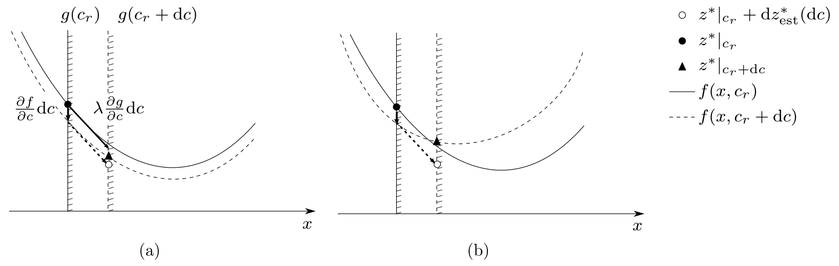
Figure 1 Illustration of the estimator on a quadratic problem, with one scalar design variable x and one constraint g, for weak (a) and strong (b) couplings.

A purely linear estimator only takes into account the linear variation in the problem with dc and cannot capture non-linear effects such as diminishing returns. Thus we propose an extension of the estimator that captures the non-linear behaviour of the constraints, called the high-order estimator. By using a higher-order expansion instead of a first-order one, the following formula is obtained:

$$\begin{array}{}\text{(9)}& \mathrm{d}{z}_{\mathrm{est}}^{*}\left(\mathrm{d}\mathit{c}\right)=\mathrm{\Delta }f\left(\mathrm{d}\mathit{c}\right)+\sum _{i\in \mathcal{I}}{\mathit{\lambda }}_i^{*}\mathrm{\Delta }{g}_i\left(\mathrm{d}\mathit{c}\right),\end{array}$$

where $\mathrm{\Delta }{g}_i\left(\mathrm{d}\mathit{c}\right)=g_i({\mathit{x}}^{*},{\mathit{c}}_{\mathrm{r}}+\mathrm{d}\mathit{c})-g_i({\mathit{x}}^{*},{\mathit{c}}_{\mathrm{r}})$, i∈ℐ, and $\mathrm{\Delta }f\left(\mathrm{d}\mathit{c}\right)=f({\mathit{x}}^{*},{\mathit{c}}_{\mathrm{r}}+\mathrm{d}\mathit{c})-f({\mathit{x}}^{*},{\mathit{c}}_{\mathrm{r}})$. The high-order estimator is valid under the following assumptions:

• the objective function and constraints are linear in x

• there are no couplings between x and c in the objective function and constraints; i.e. ${\mathrm{\nabla }}_{x,c}^{\mathrm{2}}f$ and ${\mathrm{\nabla }}_{x,c}^{\mathrm{2}}g$ are negligible

• the active set does not change with a small variation dc.

The derivation and explanation of these assumptions can be found in Appendix B. In the case that the assumptions are violated, the precision of the estimator is likely to decrease, but the method can still capture the underlying trend effects of varying the control parameter. Appendix C illustrates this aspect on a simple quadratic programme. In addition, Fig. 1 illustrates how the violation of the coupling assumption impacts the precision of the estimator. The estimated optimum (white circle) is close to the real optimum (black triangle) in the weak coupling case but less precise when the coupling is strong.

3 Case study

In this section, we present the tower design case study used to evaluate the estimator. We first describe the optimization problem on which the estimator is applied. The second part of this section focuses on the adopted linear quadratic regulator (LQR) control law and its parametrization. A description of the analysis and fatigue damage models concludes the section.

3.1 Optimization problem

We consider a wind turbine tower optimization problem with the objective of reducing the cost of energy (CoE). Two configurations of the tower design are considered: a standard configuration, where the natural frequencies of the structure are required not to interact with the rotor rotational frequency, and a soft–soft configuration, where the natural frequencies can be lower than the passing frequency, and resonance is avoided through active control. The tower design is parameterized with the tower height h, the diameter d, and the wall thickness t of each tower segment. The total tower mass is denoted by m. Geometrical constraints are set on taper, continuity of wall thickness, and maximum tower diameter. The load constraints, g_D,j, j=1, …, n_s, ensure that the fatigue damage does not exceed the value of 1 along the full length of the tower. Finally, for the standard configuration, a frequency constraint is set so that the first and second natural frequencies f₁ and f₂ are sufficiently far from the rotor 1P frequency f_1P, with a threshold δf. In this work, the controller design of the soft–soft configuration is kept simple in order to focus on the objective function sensitivity. We assume that the controller is designed in such a way as to operate immediately below and above the resonant frequency, using a classical frequency skipping approach (Bossanyi, 2000). However, for simplicity, we did not implement this feature in the controller, and we simply avoided running simulations in proximity of the resonant condition.

The optimization is represented by Eq. (10), where c=c_r represents the scalar control tuning set at its reference value:

$$\begin{array}{}\text{(10)}& \begin{array}{rl}& \underset{h}{\mathrm{minimize}}z=\mathrm{CoE}\left(m^{*}\left(h,c_{\mathrm{r}}\right),h,c_{\mathrm{r}},{\mathit{d}}^{*}\left(h,c_{\mathrm{r}}\right),{\mathit{t}}^{*}\left(h,c_{\mathrm{r}}\right)\right)\\ & \mathrm{with}{m}^{*}\left(h,c_{\mathrm{r}}\right)=\underset{\mathit{d},\mathit{t}}{\mathrm{minimize}}\left\{m(\mathit{t},\mathit{d},h),(\mathit{t},\mathit{d})\in \mathcal{S}\left(h,c_{\mathrm{r}}\right)\right\}\\ & \left[{\mathit{d}}^{*}\left(h,c_{\mathrm{r}}\right),{\mathit{t}}^{*}\left(h,c_{\mathrm{r}}\right)\right]=\underset{\mathit{d},\mathit{t}}{\mathrm{argmin}}\left\{m(\mathit{t},\mathit{d},h),\right.\\ & \left.(\mathit{t},\mathit{d})\in \mathcal{S}\left(h,c_{\mathrm{r}}\right)\right\}.\end{array}\end{array}$$

The following two sets of constraints, 𝒮₁ and 𝒮₂, are considered, corresponding to the standard and soft–soft configurations, respectively:

$$\begin{array}{}\text{(11)}& {\displaystyle }\begin{array}{rl}& (\mathit{t},\mathit{d})\in {\mathcal{S}}_{\mathrm{1}}(h,c)\leftrightarrow \\ & \left\{\begin{array}{ll}{g}_{{\mathrm{D}}_j}(\mathit{d},\mathit{t},h,c)\le \mathrm{0},& j=\mathrm{1},\mathrm{\dots },n_{\mathrm{s}}\\ f_k(\mathit{d},\mathit{t},h)\ge \frac{f_{\mathrm{1}\mathrm{P}}}{\mathrm{1}-\mathit{\delta }f,}& k=\mathrm{1},\mathrm{2}\\ \mathrm{Geometrical}\mathrm{constraints}& \end{array},\right.\end{array}\text{(12)}& {\displaystyle }\begin{array}{rl}& (\mathit{t},\mathit{d})\in {\mathcal{S}}_{\mathrm{2}}(h,c)\leftrightarrow \\ & \left\{\begin{array}{ll}{g}_{{\mathrm{D}}_j}(\mathit{d},\mathit{t},h,c)\le \mathrm{0},& j=\mathrm{1},\mathrm{\dots },n_{\mathrm{s}}\\ \mathrm{Geometrical}\mathrm{constraints}& \end{array}\right..\end{array}\end{array}$$

Equation (10) is formulated using a nested formulation, where the tower mass is the objective function of the inner optimization problem and acts as an intermediate variable to calculate the CoE. Solving the equivalent monolithic problem would require excessive computational resources. This is because a large number of aeroelastic simulations are required to accurately estimate the loads. An additional contribution to the computational cost comes form the fact that we use finite difference to estimate the gradient of the objective function and of the constraints. To limit cost, a frozen-load approach is used (Bottasso et al., 2016), where the loads are not updated within the inner optimization problem. If the change between the initial and current designs is greater than a given threshold, the aeroelastic simulations are evaluated using the current design to update the loads, and the process is iterated. This method is valid under the assumption that the load envelope varies slowly with changes in the inner tower design variables (d, t). While this approach can potentially lead to non-optimal design, it is widely used in wind energy and provides satisfying results.

3.2 Control parametrization

We use a wind-scheduled multi-input multi-output (MIMO) LQR controller with integral action (Bottasso et al., 2012b). The controller states are the tower top displacement and velocity, the rotational speed, the pitch angle, the pitch rate, and the electrical torque. The integral of the rotational speed is added to eliminate the steady-state error of the controller. The controller inputs are the pitch angle and the electrical torque. At each wind speed considered, the controller gains are computed by applying LQR theory to the linearized system of the turbine dynamics; see Hendricks et al. (2008) for more details.

The tuning of an LQR controller is done through the choice of the entries of the weight matrices associated with the states and inputs, noted Q and R. In this work, the controller is tuned by changing the diagonal term of Q associated with the tower top velocity, labelled c. The following expression reports the parametrization of the weight matrices:

$$\begin{array}{}\text{(13)}& \begin{array}{rl}& \mathbf{Q}\left(c\right)=\left[\begin{array}{ccccccc}\mathrm{0}& & & & & & \\ & c& & & & & \\ & & \mathrm{0}& & & & \\ & & & \frac{\mathrm{1}}{{\mathit{\beta }}_{\max }^{\mathrm{2}}}& & & \\ & & & & \mathrm{0}& & \\ & & & & & \mathrm{0}& \\ & & & & & & q\end{array}\right],\mathbf{R}=\left[\begin{array}{cc}r& \mathrm{0}\\ \mathrm{0}& \mathrm{0.1}\end{array}\right],\\ & \mathrm{with}\left\{\begin{array}{l}q=\min (\mathrm{0.1},\mathrm{0.015}\cdot (V-\mathrm{3})+\mathrm{0.01})\\ r=\min (\mathrm{1.0},\max (\mathrm{0.1},\mathrm{1}-\mathrm{0.18}\cdot (V-\mathrm{9})\left)\right),\end{array}\right.\end{array}\end{array}$$

where β_max is the maximum pitch angle of the turbine power regulation strategy. The parameters r and q are used for gain scheduling and are varied according to the wind speed V. The reference value for the control tuning is c_r=0.

Figure 2 shows that, by varying the only free parameter c, the average fatigue damage can be reduced by up to 6.8 %. However, the fatigue damage reduction varies depending on where the fatigue damage constraint is calculated on the tower.

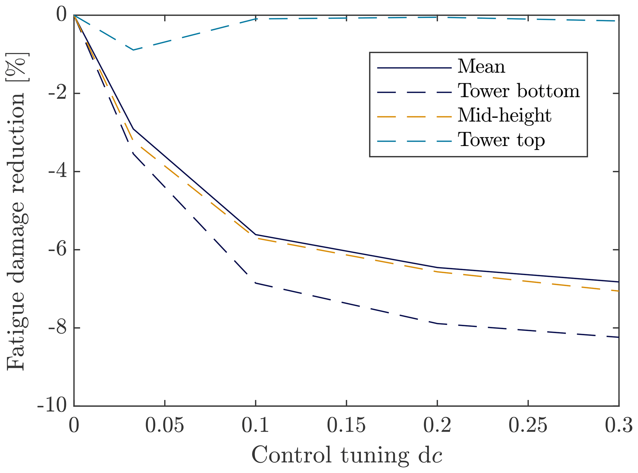
Figure 2 Impact of the control tuning on the mean fatigue damage and at three locations along the tower.

3.3 Analysis model

The numerical experiments presented in this work are conducted using the multi-disciplinary wind turbine design optimization framework Cp-max. The details of the framework can be found in the available literature (Bottasso et al., 2012a, 2014, 2016). We highlight the aspects that are important for the tower design optimization and fatigue calculations in this section.

The tower is modelled as a steel tubular structure, divided into n_e elements. Each tower element is characterized by its radius at the top and bottom and its wall thickness. The tower is then modelled as a non-linear geometrically exact shear- and torsion-deformable beam. This is used in turn in the multi-body model of the wind turbine for the aeroelastic simulations, using the solver Cp-Lambda. The aerodynamics of the wind turbine are modelled using the blade element momentum method.

The fatigue load analysis is performed according to certification standards (International Electrotechnical Commission, 2005). Simulations are run from the cut-in to the cut-out wind speed with increments of 2 m s⁻¹. At each considered wind speed, a turbulent wind field is generated with TurbSim (Jonkman, 2009). Simulations are run for 600 s for six different turbulent seeds, excluding an initial transient period of 30 s. Once the aeroelastic simulations are run, loads are extracted at n_s stations along the tower to compute the stress loading on the structure. A rain-flow counting algorithm is then used on the stress time history to identify the number of loading cycles and their amplitude. Miner's rule and the material S–N curve are used to estimate the lifetime fatigue damage at each station (Sutherland, 1999).

The cost of energy is calculated following the NREL cost model (Fingersh et al., 2006):

$$\begin{array}{}\text{(14)}& \mathrm{CoE}(m,h,c,\mathit{d},\mathit{t})={\displaystyle \frac{\mathrm{FCR}\cdot \mathrm{ICC}\left(m\right)}{{\mathrm{AEP}}^{\mathrm{net}}(h,c,\mathit{d},\mathit{t})}}+\mathrm{AOE},\end{array}$$

where the fixed charged rate (FCR) and the annual operating expenses (AOEs) are assumed to be independent of the design variables. The initial capital cost (ICC) varies only with the tower mass m (which, in turn, depends on the tower height h, controller tuning c, and inner tower design variables d and t), since the rest of the wind turbine design is assumed fixed. Finally, the net annual energy production (AEP^net) is calculated from aeroelastic simulations.

4 Application of the estimation method to the case study

This section describes how the first-order and high-order estimation formulas derived in Sect. 2 are applied to the tower design optimization problem to estimate the benefits of a control co-design approach. In principle, Eq. (10) could be promising for a CCD approach since the control tuning c has a direct impact on the dynamic response of the wind turbine, which in turn influences fatigue loads. As a result, it is reasonable to expect that the integrated design of control and tower could improve the design through reductions in the fatigue damage constraints.

The estimation formulas presented in Sect. 4 are derived from a monolithic optimization problem, not a nested one. Therefore, it is not possible to apply it directly to Eq. (10). Instead, we apply Eqs. (8) and (9) to the nested optimization problem, which is monolithic. Regarding the validity assumptions of the high-order estimator, a preliminary study on the impact of the control tuning on the fatigue damage constraint ensured the robustness of the active set with the chosen range of control tuning variation. In addition, the objective and constraints can be assumed to be linear in x provided the change in design is small. However, the validity assumption related to the coupling is more difficult to prove due to the complexity of the problem considered. Therefore, the high-order estimator may be unprecise.

The objective function for the considered problem is $m(\mathit{t},\mathit{d},h)$ and does not depend on the control parameter. Therefore the first term in the estimator equations is 0: ${\mathrm{\nabla }}_{\mathrm{c}}f={\mathrm{\nabla }}_{\mathrm{c}}m=\mathrm{0}$ and $\mathrm{\Delta }f\left(\mathrm{d}c\right)=\mathrm{\Delta }m\left(\mathrm{d}c\right)=\mathrm{0}$. Among the constraints of the problem, the fatigue damage constraint is the only one impacted by the tuning of the controller. Therefore, the second term of the estimation formulas only depends on g_D,j, j=1, …, n_s. This leads to the following estimate functions for the change in optimal tower mass:

$$\begin{array}{}\text{(15)}& \mathrm{d}{m}_{\mathrm{est}}^{*}\left(\mathrm{d}c\right)=\left\{\begin{array}{ll}\sum _{j=\mathrm{1}}^{n_{\mathrm{s}}}{\mathit{\lambda }}_{\mathrm{D},j}{\mathrm{\nabla }}_{\mathrm{c}}{g}_{\mathrm{D},j}\mathrm{d}c& \mathrm{first}\mathrm{order}\\ \sum _{j=\mathrm{1}}^{n_{\mathrm{s}}}{\mathit{\lambda }}_{\mathrm{D},j}\mathrm{\Delta }{g}_{\mathrm{D},j}\left(\mathrm{d}c\right)& \mathrm{high}\mathrm{order},\end{array}\right.\end{array}$$

where λ_D,j represents the Lagrange multipliers of the inner problem associated with the fatigue damage constraint g_D,j. The Lagrange multipliers are obtained by solving the nested optimization at the reference value of the control parameter c_r. The terms ∇_cg_D,j and Δg_D,j(dc) are calculated by running aeroelastic simulations and evaluating the fatigue damage for different values of dc and using the optimal tower design (d^*, t^*) obtained with the reference control tuning. The terms ∇_cg_D,j are evaluated using forward finite differences with a step of 0.03.

While the estimator formula cannot be applied directly to the outer optimization problem, it can inform on the sensitivity of CoE with regard to control changes. In Eq. (14), CoE depends on the controller tuning for the calculation of the AEP and the ICC through the optimal tower mass m^*. However, the net annual energy production is mostly driven by the tower height, whereas the impact of the controller tuning and the inner tower design is marginal in comparison: ${\mathrm{AEP}}^{\mathrm{net}}(h,c,\mathit{d},\mathit{t})\simeq {\stackrel{\mathrm{̃}}{\mathrm{AEP}}}_{\mathrm{est}}^{\mathrm{net}}\left(h\right)$. The following CoE estimate is written as a function of tower height and control tuning only:

$$\begin{array}{}\text{(16)}& \begin{array}{rl}{\mathrm{CoE}}_{\mathrm{est}}(h,\mathrm{d}c)& ={\displaystyle \frac{\mathrm{FCR}\cdot \mathrm{ICC}\left(m_{\mathrm{est}}^{*}\left(h,c_{\mathrm{r}}+\mathrm{d}c\right)+\mathrm{d}{m}_{\mathrm{est}}{|}_h\left(\mathrm{d}c\right)\right)}{{\stackrel{\mathrm{̃}}{\mathrm{AEP}}}_{\mathrm{est}}^{\mathrm{net}}\left(h\right)}}\\ & +\mathrm{AOE}.\end{array}\end{array}$$

The term dm_est is varied with the tower height. The Lagrange multipliers are updated with h. However, the change in fatigue damage constraints is calculated for the reference tower height h₀ only, assuming that the term is relatively insensitive to height changes.

This function can be used to gauge the optimal CoE that would have been obtained by solving the minimization problem including control tuning as a design variable, i.e. using CCD. This is done by minimizing the CoE estimate with respect to h and dc:

$$\begin{array}{}\text{(17)}& {\mathrm{CoE}}_{\mathrm{est}}^{*}=\underset{h,\mathrm{d}c}{\mathrm{minimize}}{\mathrm{CoE}}_{\mathrm{est}}(h,\mathrm{d}c).\end{array}$$

5 Results

In this section, the estimation method presented in Sect. 4 is applied to redesign the tower of the IEA 3.4 MW reference onshore wind turbine (Bortolotti et al., 2019). We compare the high-order estimator of the optimal tower mass and CoE to optimization results. The computational effort of the estimation method is reported at the end of the section.

All optimization problems are solved using the active-set optimization algorithm implemented in the fmincon routine of MATLAB (The MathWorks Inc., 2019). The outer optimization is solved with a tolerance on the expected objective function change ${\mathit{ϵ}}_{\mathrm{obj}}={\mathrm{10}}^{-\mathrm{5}}$. The inner optimization is solved with ${\mathit{ϵ}}_{\mathrm{obj}}={\mathrm{10}}^{-\mathrm{4}}$ and with a tolerance on constraint violation ${\mathit{ϵ}}_{\mathrm{con}}={\mathrm{10}}^{-\mathrm{2}}$. The objective functions for the outer and inner problems are both scaled by the corresponding value of the initial design. The number of tower elements is n_e=10, and the number of fatigue damage constraints is n_s=19. The threshold for the frozen-load method is set to 1 %.

5.1 Estimator performance on the optimal tower mass

In this section, the change in optimal tower mass due to a control tuning variation is estimated. Then, this estimate is compared to the solution of the tower mass optimization problem run for different variations in the control parameter at the reference tower height.

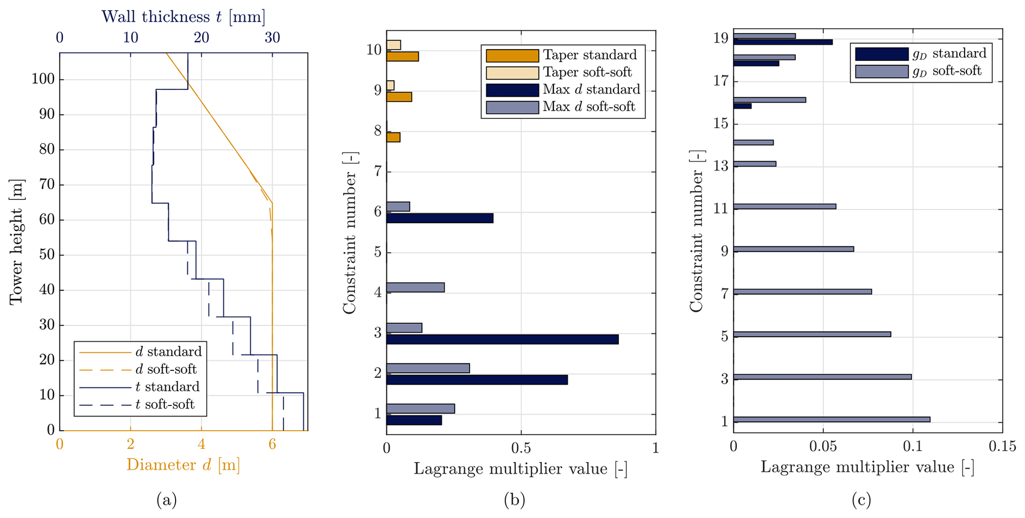
Figure 3 Characteristics of the optimal standard and soft–soft tower designs for the reference height h_r=110 m and control tuning c=0: optimal tower design (a) optimal Lagrange multipliers associated with the geometric (b) and fatigue damage constraints (c).

We first look at the importance of the different constraints on the design by solving the inner tower optimization problem with fixed control tuning c=0 and fixed tower height h_r=110 m. Figure 3 reports the optimal design and the Lagrange multipliers for the two considered configurations. For both configurations, the designs are similar. However, the presence of the frequency constraints in the standard configuration drives the wall thickness up in the bottom half of the tower. Analysis of the Lagrange multiplier shows that for the soft–soft configuration, geometric constraints are the primary drivers. However, these constraints are also insensitive to control tuning. The next most important constraint is fatigue, which can be mitigated by control, indicating potential benefits from CCD. In the standard configuration, the largest Lagrange multiplier is associated with the added frequency constraint, with λ_f=2.44. The Lagrange multipliers associated with fatigue are 1 order of magnitude smaller, showing a lower relative importance of these constraints and a reduced potential for CCD compared to the soft–soft case.

Using the value of the Lagrange multipliers, the first-order and high-order estimators are calculated and reported in Fig. 4. The results of the optimization for dc=0.1, 0.2, and 0.3 are also reported. The high-order estimator accurately predicts the change in optimal mass for the standard configuration, whereas it under-predicts the results for the soft–soft configuration. Both estimators are able to show that the soft–soft configuration benefits significantly more from a change in control tuning than the standard one, in accordance with the constraint analysis. However, the high-order estimator more precisely quantifies this benefit, whereas the first-order estimator fails to capture the effect of diminishing returns on controller tuning.

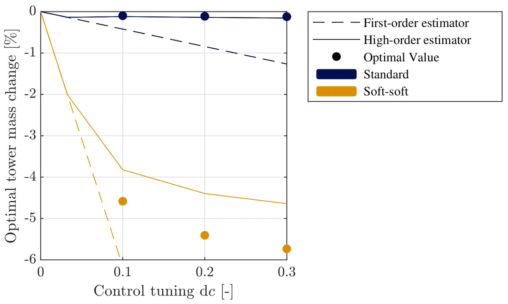
Figure 4 Comparison between the optimum mass change dm^* and the estimated mass change $\mathrm{d}{m}_{\mathrm{est}}^{*}$ calculated with the first-order and high-order estimator, for different values of the control parameter and for the two configurations. The tower height is fixed to the reference height.

5.2 Estimator performance on the CoE

In this section, we want to understand if the CoE can be reduced by the combined action of control load alleviation and changed tower height through CCD and if the proposed estimation method can predict the CCD results.

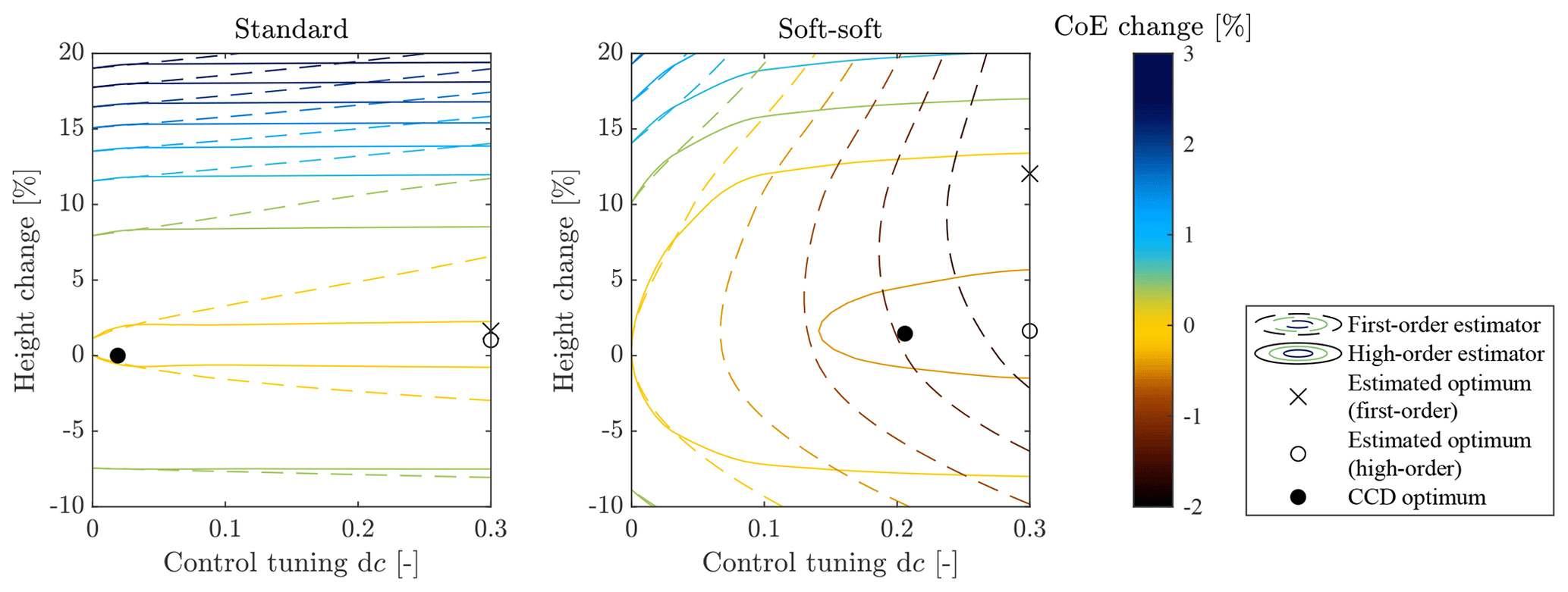
Figure 5 Relative change in CoE as a function of the tower height change and control tuning parameter calculated using the first-order and high-order estimators, for the standard and soft–soft configuration. The reference CoE is the optimal value for the non-CCD problem with c=0.

Figure 5 reports the contour plot of the CoE estimate function for the standard and soft–soft configurations, calculated as described in Sect. 4 for different tower heights (0.9 h_r, h_r, 1.1 h_r, 1.2 h_r) and for dc=0, 0.03, 0.1, 0.2, 0.3. Both the first-order and the high-order estimate functions are represented. As expected, there is little coupling between the tower height and the control parameter in the standard configuration, with the CoE showing only marginal variations with control tuning. For the soft–soft configuration instead, the CoE can be reduced by simultaneously changing the control parameter and the tower height. The estimated change in optimal CoE is calculated as the minimum of the estimate function and marked in Fig. 5 as a cross and a white circle for the first-order and high-order methods, respectively.

In order to assess the accuracy of the CoE estimator, we solve the tower optimization problem with a non-CCD formulation (corresponding to Eq. 10 with c=0) and with a CCD formulation where the control tuning is bounded between 0 and 0.3. Table 1 reports the change in optimal CoE brought by the use of CCD calculated directly with the optimization results and with the estimation method (first order and high order). The two estimation methods correctly predict that the soft–soft configuration benefits much more from CCD than the standard configuration. In addition, the estimated improvement is accurate in the high-order case compared to the optimization results. Instead, the first-order estimator significantly over-predicts the benefits of CCD, which is in agreement with the limitations of the approach. We note that the estimated change in optimal design is far from the actual one in Fig. 5. This is in agreement with the goal of the presented method to quantify the sensitivity of the optimal objective value and not of the optimum.

Table 1 Percentage improvement in the optimal CoE using a CCD approach, calculated with optimization results and the estimation method.

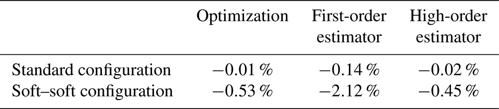
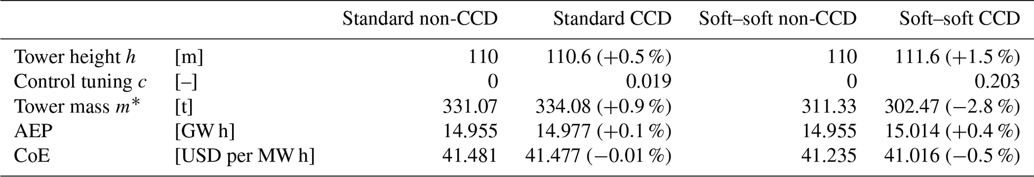
Table 2 documents the optimization results used to compute the data in Table 1. The data show that the optimal CCD soft–soft tower is 2.8 % lighter and 1.5 % higher than the version calculated without CCD, which implies a gain in power capture in sheared inflow. This reduction in tower mass and increase in power capture explain why the CoE is more impacted for the soft–soft configuration than for the standard configuration.

Table 2 Characteristics of the optimal design for the non-CCD and CCD problems and for the standard and soft–soft configuration. The percentage change between the CCD and the non-CCD cases is reported in parentheses.

5.3 Computational effort

In terms of computational costs, calculating the high-order estimator requires evaluating (i) the Lagrange multipliers by solving the optimization problem at the reference control and (ii) the constraints for different values of the control parameter. In this section, we compare this computational effort to the one needed to solve the CCD optimization problem, applied to the CoE.

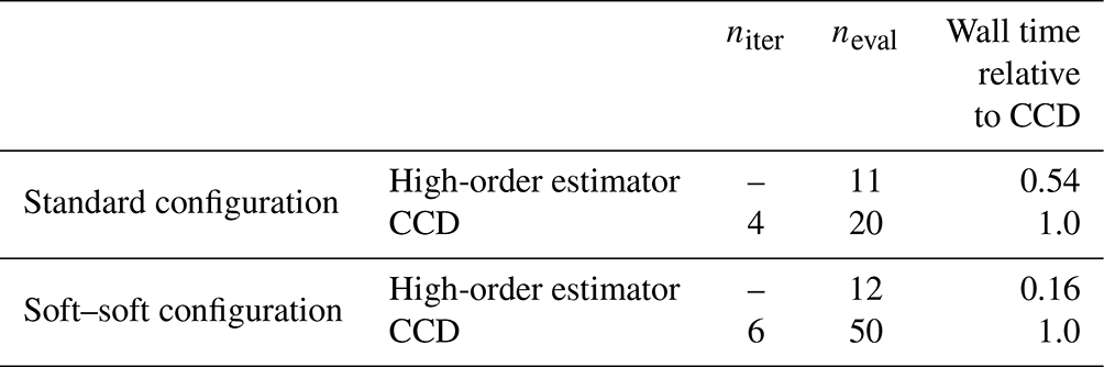
Table 3 reports different metrics to compare the computational cost between the high-order estimator and the CCD optimization. The number of evaluations of the full set of aeroelastic simulations, noted n_eval, is used as the main comparison metric, since it is the most computationally expensive step of the design process. The fatigue damage constraints are evaluated for four different values of the control tuning and require one full-set evaluation each. The Lagrange multipliers are evaluated for four different tower heights and require between one and two full-set evaluations each, depending on the number of iterations in the frozen-load loop. As a result, the estimator is calculated using a total of 11 or 12 full-set evaluations depending on the configuration. Instead, the CCD optimization requires 20 and 50 full-set evaluations for the standard and soft–soft configurations, respectively. In terms of wall time, the estimation method is computed in around half and a sixth of the time required to solve the CCD problem for the two configurations. Therefore, the presented estimation method is computationally efficient. We note that the number of iterations for the outer optimization for the two CCD cases is low. For more complex problems or when using a tighter optimization tolerance, the number of iterations is likely to increase significantly, and the computational effort of the CCD process will also increase.

Table 3 Computational effort for the CoE estimator and for the CCD optimization: number of iterations for the outer optimization n_iter, number of evaluations of the full set of aeroelastic simulations n_eval, and wall time relative to the CCD case.

6 Discussion

A CCD approach can incur major computational costs when compared to the simpler non-CCD optimization. At the same time, our results show that CCD is not always guaranteed to provide benefits to the final design compared to a more straightforward non-CCD approach. Without knowing a priori the potential benefit, there is a significant risk, in terms of engineering time, code development, and computational resources, in attempting a CCD optimization. This work suggests that results from the simplified optimization problem can be used in conjunction with the high-order estimator to determine whether a given problem can benefit from a CCD approach. The first-order estimator shows similar results, with a reduced precision. Furthermore, the analysis of the Lagrange multipliers and constraint sensitivity in the proposed method gives a justification for why a CCD approach would fail. This information is generally not readily available when running a CCD optimization directly because optimization algorithms can fail for technical reasons (inadequate parameters, scaling, or problem formulation).

The method is applicable to similar problems where the optimum design is driven by a load constraint, when loads can be alleviated by control action (for example, the design of wind turbine support structures or blades). The computational cost reduction should be similar in problems where the fatigue damage constraints are driving the design. In cases where the driving constraints are easier to evaluate, there should be a greater reduction in computational effort, since the estimator would be less expensive to compute. In addition, while the estimation method was developed to target CCD applications, the mathematical derivations and associated assumptions are developed in the general case, where c can be any parameter. Therefore, it can be applied to any optimization problem to disentangle the effects of one parameter from the rest of the solution.

The precision of the high-order estimator depends on several assumptions on the objective functions and constraints. When the assumptions are violated, the estimator can under-predict the benefits of CCD, as shown in our results. In addition, the estimator uses local sensitivity information of the non-CCD optimum, and therefore it will be inaccurate when a CCD approach significantly changes the design. Consequently, there may still be a benefit of using a CCD approach, even if the estimator fails to show it.

In this study, we perform CCD using one tuning parameter of the LQR controller. However, the proposed method is general and does not depend on the control architecture. The applicability of the method to parametrizations with a large number of design variables is left for future work on the topic.

Finally, this work shows how CCD can be used for the design of wind turbine towers. In the presence of an active frequency constraint, CCD may not give significant improvements. Instead, the use of active load alleviation enables a taller and lighter-mass tower compared to the non-CCD design. Our results are specific to one particular wind turbine and may not be generally applicable. Notwithstanding these limitations, the results reported here highlight the importance of performing a thorough analysis of the driving constraints through the use of Lagrange multipliers before attempting a complex and computationally expensive optimization.

7 Conclusion

This study shows how design sensitivity analysis can be used to estimate the change in optimal objective value caused by a change in control. Using the solution of an optimization problem with fixed control, we can characterize the results of the more complex control co-design problem without the associated computational effort. Two estimators are presented, based on first-order and high-order approximations, where the latter captures non-linear effects.

The proposed estimation method is applied to the redesign of a wind turbine tower driven by fatigue loads, using an LQR controller targeting fatigue load alleviation. High computational resources are required to calculate fatigue damage accurately, which makes this problem an ideal application for the estimator. Two design configurations are considered: a standard configuration, where a frequency constraint is enforced to avoid resonance with the rotational frequency of the rotor, and a soft–soft configuration, where resonance is avoided using active control. The proposed first-order and high-order estimators are applied to the optimal tower mass and optimal CoE problems. We have shown that the high-order estimator accurately predicts how the tower mass changes with control tuning compared to optimization results. The first-order estimator is inaccurate for large values of control tuning but captures the difference between the standard and soft–soft configurations. Combined with a simple CoE model, the high-order estimator predicts a 0.45 % reduction in optimal CoE for the soft–soft tower, while running the CCD optimization gives an improvement of 0.53 %. The proposed estimation method is accurate and uses only a fraction of the computational resources of the CCD optimization. Our results additionally show that the standard tower configuration does not benefit from a CCD approach due to the presence of an active frequency constraint. Changing the control is beneficial for the soft–soft tower because the fatigue damage constraint is the primary design driver and can be alleviated by control action. In this case, the use of CCD yields a taller tower with lower mass, which impacts the CoE significantly.

As shown in this work, design sensitivity analysis allows one to identify relevant design problems for CCD from the results of a simplified non-CCD solution. In a context where computational effort is an obstacle to the wide use of CCD, the proposed method can help identify and quantify the benefits of this approach for wind energy applications.

Appendix A: Nomenclature

Symbols used for generic optimization problems
λ	Lagrange multipliers
c or c	Variables or parameters describing the
	controller
cr or cr	Reference value for the control variables
f	Objective function
gi, i=1, …, n	Constraints
x	Design variable of the optimization
	problem, except control
z	Objective function value
ℐ	Set of active constraints
∇x□	Jacobian or gradient of □ with regards
	to x
${\square }^{*}$	Value at the optimum
d□	Small variation

d□est	Estimated value of the variation
	in □
Symbols used for the tower design optimization problem
λD,j, j=1, …, ns	Lagrange multipliers associated
	with the fatigue damage constraint
λf	Lagrange multipliers associated
	with the first frequency constraint
d	Diameter of the tower elements
f1, f2, f1P	First and second natural
	frequencies of the turbine and
	rotor 1P passing frequency
gD,j, j=1, …, ns	Fatigue damage constraints
h	Tower height
m	Mass of the tower
ne, ns	Number of tower elements and
	fatigue damage constraints
r, q	Gain-schedule parameters for the
	LQR control gains
t	Thickness of the tower elements
Abbreviations
AEP	Annual energy production
AOEs	Annual operating expenses
CCD	Control co-design
CoE	Cost of energy
FCR	Fixed charge rate
ICC	Investment capital cost
LQR	Linear quadratic regulator

Appendix B: High-order estimator

In this appendix, we derive the high-order estimator expressed by Eq. (9) and explain the validity assumptions, listed below:

• A1. The objective function and constraints are linear in x.

• A2. There are no couplings between x and c in the objective function and constraints; i.e. ${\mathrm{\nabla }}_{x,\mathrm{c}}^{\mathrm{2}}f$ and ${\mathrm{\nabla }}_{x,\mathrm{c}}^{\mathrm{2}}g$ are negligible.

• A3. The active set does not change with a small variation dc.

We consider the following non-linear optimization problem:

$$\begin{array}{}\text{(B1)}& \begin{array}{rl}& \underset{\mathit{x}}{\mathrm{minimize}}z=f\left(\mathit{x},{\mathit{c}}_{\mathrm{r}}\right)\\ & \mathrm{subject}\mathrm{to}{g}_i\left(\mathit{x},{\mathit{c}}_{\mathrm{r}}\right)\le \mathrm{0}i=\mathrm{1},\mathrm{\dots },n.\end{array}\end{array}$$

The change in optimal objective value due to a change in the control parameter dc is defined as

$$\begin{array}{}\text{(B2)}& \mathrm{d}{z}^{*}\left(\mathrm{d}\mathit{c}\right)=f\left({\mathit{x}}^{*}+\mathrm{d}{\mathit{x}}^{*},{\mathit{c}}_{\mathrm{r}}+\mathrm{d}\mathit{c}\right)-f\left({\mathit{x}}^{*},{\mathit{c}}_{\mathrm{r}}\right).\end{array}$$

We assume that the objective function f is linear in x (A1) and does not have a coupling between the variables x and c (A2). Using these assumptions on a second-order Taylor expansion of Eq. (B2) gives

$$\begin{array}{}\text{(B3)}& \begin{array}{rl}\mathrm{d}{z}^{*}\left(\mathrm{d}\mathit{c}\right)& =f\left({\mathit{x}}^{*}+\mathrm{d}{\mathit{x}}^{*},{\mathit{c}}_{\mathrm{r}}+\mathrm{d}\mathit{c}\right)-f\left({\mathit{x}}^{*},{\mathit{c}}_{\mathrm{r}}\right)\\ & ={\mathrm{\nabla }}_{x}f{\left({\mathit{x}}^{*},{\mathit{c}}_r\right)}^T\mathrm{d}{\mathit{x}}^{*}+{\mathrm{\nabla }}_{\mathrm{c}}f{\left({\mathit{x}}^{*},{\mathit{c}}_{\mathrm{r}}\right)}^T\mathrm{d}\mathit{c}\\ & +{\displaystyle \frac{\mathrm{1}}{\mathrm{2}}}\mathrm{d}{\mathit{x}}^{{*}^T}{\mathrm{\nabla }}_x^{\mathrm{2}}f\left({\mathit{x}}^{*},{\mathit{c}}_{\mathrm{r}}\right)\mathrm{d}{\mathit{x}}^{*}\\ & +{\displaystyle \frac{\mathrm{1}}{\mathrm{2}}}\mathrm{d}{\mathit{c}}^T{\mathrm{\nabla }}_{\mathrm{c}}^{\mathrm{2}}f\left({\mathit{x}}^{*},{\mathit{c}}_{\mathrm{r}}\right)\mathrm{d}\mathit{c}\\ & +\mathrm{d}{\mathit{x}}^{{*}^T}{\mathrm{\nabla }}_{x\mathrm{c}}^{\mathrm{2}}f\left({\mathit{x}}^{*},{\mathit{c}}_{\mathrm{r}}\right)\mathrm{d}\mathit{c}+o\left(\left|\right|\mathrm{d}\mathit{c}|{|}^{\mathrm{2}}\right).\end{array}\end{array}$$

We use the notation ${\mathrm{\nabla }}_x^{\mathrm{2}}\square$ for the Hessian of a function with respect to x. Due to the assumptions A1 and A2 on f, the second-order terms dependent on dx^* are negligible. The remaining terms dependent on dc can be identified with the second-order Taylor expansion of the function $\mathit{c}\mapsto f({\mathit{x}}^{*},\mathit{c})$ around the point c=c_r. Therefore, the expression can be rewritten as

$$\begin{array}{}\text{(B4)}& \mathrm{d}{z}^{*}\left(\mathrm{d}\mathit{c}\right)={\mathrm{\nabla }}_{x}f{\left({\mathit{x}}^{*},{\mathit{c}}_{\mathrm{r}}\right)}^T\mathrm{d}{\mathit{x}}^{*}+\mathrm{\Delta }f\left(\mathrm{d}\mathit{c}\right)+o\left(\left|\right|\mathrm{d}\mathit{c}|{|}^{\mathrm{2}}\right),\end{array}$$

where $\mathrm{\Delta }f\left(\mathrm{d}\mathit{c}\right)=f({\mathit{x}}^{*},{\mathit{c}}_{\mathrm{r}}+\mathrm{d}\mathit{c})-f({\mathit{x}}^{*},{\mathit{c}}_{\mathrm{r}})$. Assumptions A1 and A2 on the constraints lead to the following expression:

$$\begin{array}{}\text{(B5)}& \begin{array}{rl}{g}_i& \left({\mathit{x}}^{*}+\mathrm{d}{\mathit{x}}^{*},{\mathit{c}}_{\mathrm{r}}+\mathrm{d}\mathit{c}\right)-g_i\left({\mathit{x}}^{*},{\mathit{c}}_{\mathrm{r}}\right)={\mathrm{\nabla }}_x{g}_i{\left({\mathit{x}}^{*},{\mathit{c}}_{\mathrm{r}}\right)}^T\mathrm{d}{\mathit{x}}^{*}\\ & +\mathrm{\Delta }{g}_i\left(\mathrm{d}\mathit{c}\right)+o\left(\left|\right|\mathrm{d}\mathit{c}|{|}^{\mathrm{2}}\right),i=\mathrm{1},\mathrm{\dots },n,\end{array}\end{array}$$

where $\mathrm{\Delta }{g}_i\left(\mathrm{d}\mathit{c}\right)=g_i({\mathit{x}}^{*},{\mathit{c}}_{\mathrm{r}}+\mathrm{d}\mathit{c})-g_i({\mathit{x}}^{*},{\mathit{c}}_{\mathrm{r})}$, i=1, …, n. We consider the set ℐ of active constraints. Assuming that the active set does not change with dc (A3), one has $g_i({\mathit{x}}^{*}+\mathrm{d}{\mathit{x}}^{*}$, ${\mathit{c}}_{\mathrm{r}}+\mathrm{d}\mathit{c})=g_i({\mathit{x}}^{*}$, c_r)=0, i∈ℐ, and therefore

$$\begin{array}{}\text{(B6)}& {\displaystyle }{\mathrm{\nabla }}_x{g}_i{\left({\mathit{x}}^{*},{\mathit{c}}_{\mathrm{r}}\right)}^T\mathrm{d}{\mathit{x}}^{*}=-\mathrm{\Delta }{g}_i\left(\mathrm{d}\mathit{c}\right)+o\left(\left|\right|\mathrm{d}\mathit{c}|{|}^{\mathrm{2}}\right),i\in \mathcal{I}.\end{array}$$

We can relate the gradient of the objective function to the gradient of the constraints using the optimality conditions. We assume that f and g_i, i=1, …, n are differentiable and that strong duality holds for Eq. (B1). Then, if x^* is optimal, there is a set of Lagrange multipliers λ^* satisfying the Karush–Kuhn—Tucker conditions (Boyd and Vandenberghe, 2004). Among these, the stationarity condition states

$$\begin{array}{}\text{(B7)}& {\mathrm{\nabla }}_{x}f\left({\mathit{x}}^{*},{\mathit{c}}_{\mathrm{r}}\right)+{\left({\mathit{\lambda }}^{*}\right)}^T{\mathrm{\nabla }}_x\mathit{g}\left({\mathit{x}}^{*},{\mathit{c}}_{\mathrm{r}}\right)=\mathbf{0}.\end{array}$$

The stationarity condition is reformulated by post-multiplying it by dx^* and by separating active and inactive constraints:

$$\begin{array}{}\text{(B8)}& \begin{array}{rl}{\mathrm{\nabla }}_{x}f{\left({\mathit{x}}^{*},{\mathit{c}}_{\mathrm{r}}\right)}^T\mathrm{d}{\mathit{x}}^{*}& =-\sum _{i\notin \stackrel{\mathrm{‾}}{\mathcal{I}}}{\mathit{\lambda }}_i^{*}{\mathrm{\nabla }}_x{g}_i{\left({\mathit{x}}^{*},{\mathit{c}}_{\mathrm{r}}\right)}^T\mathrm{d}{\mathit{x}}^{*}\\ & -\sum _{i\in \mathcal{I}}{\mathit{\lambda }}_i^{*}{\mathrm{\nabla }}_x{g}_i{\left({\mathit{x}}^{*},{\mathit{c}}_{\mathrm{r}}\right)}^T\mathrm{d}{\mathit{x}}^{*}.\end{array}\end{array}$$

The terms corresponding to inactive constraints are 0 since λ_i=0. The terms corresponding to active constraints can be reformulated using Eq. (B6). Following these considerations, Eq. (B8) becomes

$$\begin{array}{}\text{(B9)}& {\mathrm{\nabla }}_{x}f{\left({\mathit{x}}^{*},{\mathit{c}}_{\mathrm{r}}\right)}^T\mathrm{d}{\mathit{x}}^{*}=\sum _{i\in \mathcal{I}}{\mathit{\lambda }}_i^{*}\mathrm{\Delta }{g}_i\left(\mathrm{d}\mathit{c}\right)+o\left(\left|\right|\mathrm{d}\mathit{c}|{|}^{\mathrm{2}}\right).\end{array}$$

The expression for ${\mathrm{\nabla }}_{x}f({\mathit{x}}^{*},{\mathit{c}}_{\mathrm{r}}{)}^T\mathrm{d}{\mathit{x}}^{*}$ in Eq. (B4) can be replaced by Eq. (B9), which gives the equation for the high-order estimator:

$$\begin{array}{}\text{(B10)}& \mathrm{d}{z}^{*}\left(\mathrm{d}\mathit{c}\right)=\sum _{i\in \mathcal{I}}{\mathit{\lambda }}_i^{*}\mathrm{\Delta }{g}_i\left(\mathrm{d}\mathit{c}\right)+\mathrm{\Delta }f\left(\mathrm{d}\mathit{c}\right)+o\left(\left|\right|\mathrm{d}\mathit{c}|{|}^{\mathrm{2}}\right).\end{array}$$

The first term of the formula can be expanded to all constraints instead of the set ℐ since ${\mathit{\lambda }}_i^{*}=\mathrm{0}$ for inactive constraints. Furthermore, the high-order estimator formula is derived here using a second-order Taylor expansion. However, we can repeat the reasoning with an arbitrary high-order k of the Taylor expansion, resulting in an expression in $o\left(\right|\left|\mathrm{d}\mathit{c}\right|{|}^k)$ instead of $o\left(\right|\left|\mathrm{d}\mathit{c}\right|{|}^{\mathrm{2}})$.

Appendix C: Application to a quadratic programme

In this section, we illustrate how the assumptions associated with the high-order estimator impact its validity. For this purpose, we study the simple quadratic programme below, with $\mathit{x}=[x_{\mathrm{1}},x_{\mathrm{2}}{]}^T$:

$$\begin{array}{}\text{(C1)}& \begin{array}{rl}& \underset{\mathit{x}}{\mathrm{minimize}}z={\mathit{y}}^T\mathbf{P}\mathit{y}+{\mathit{q}}^T\mathit{y}+z_{\mathrm{0}},\mathrm{where}\mathit{y}=[\mathit{x},c{]}^T\\ & \mathrm{subject}\mathrm{to}\mathbf{G}\mathit{x}\le g_{\mathrm{2}}{c}^{\mathrm{2}}+g_{\mathrm{1}}c+g_{\mathrm{0}}\\ & \mathbf{H}\mathit{x}\le h_{\mathrm{0}}.\end{array}\end{array}$$

The values of P, q, G, g_i, i=0, … ,2, H, and h₀ can be adjusted to create problems that satisfy or violate the validity assumption for the estimator. The parameter z₀ is set so that the optimal objective value of the reference problem is $z^{*}=\mathrm{0}$. For each type of problem, we study how the optimum and the estimator $\mathrm{d}{z}_{\mathrm{est}}^{*}$ change with the value of dc. The reference problem is always taken for c=0, and dc varies between 0 and 1.

A1: the objective function is linear in x

In order to represent problems with objective functions linear or non-linear in x, the diagonal terms of the matrix P are varied with a parameter b. We use the following:

$$\begin{array}{}\text{(C2)}& \begin{array}{rl}\mathbf{P}=& \left[\begin{array}{ccc}b& \mathrm{0}& \mathrm{0}\\ \mathrm{0}& b& \mathrm{0}\\ \mathrm{0}& \mathrm{0}& \mathrm{0}\end{array}\right],\mathit{q}=\left[\begin{array}{c}-\mathrm{10}\\ \mathrm{1}\\ \mathrm{0}\end{array}\right],\mathbf{G}=\left[\begin{array}{cc}\mathrm{1}& \mathrm{0}\end{array}\right],\\ & g_{\mathrm{2}}=-\mathrm{4},g_{\mathrm{1}}=\mathrm{3},g_{\mathrm{0}}=\mathrm{1},\mathbf{H}=\mathbf{0},h_{\mathrm{0}}=\mathrm{0}.\end{array}\end{array}$$

When b=0, the objective function is strictly linear in x. With increasing values of b, the non-linear terms in the objective function dominate the linear term more and more. We study how the estimator performs for b=20, 5, and 0.1. For this problem, the objective function is not dependent on c.

Figure C1 shows the value of the objective as a function of x₁ and x₂. The constraint $\mathbf{G}\mathit{x}\le g_{\mathrm{2}}{c}^{\mathrm{2}}+g_{\mathrm{1}}c+g_{\mathrm{0}}$ is represented for different values of c as a yellow line, and the optimum is marked as an asterisk. The figure shows that the optimal design changes in a similar way for the different values of b. Figure C2 reports the value of the optimum change dz^* and of the first-order and high-order estimator $\mathrm{d}{z}_{\mathrm{est}}^{*}$ for the different values of b. For low values of b when the objective function is mostly linear in x, the high-order estimator follows the optimal value more closely. In addition, we observe that the first-order estimator follows the slope of the optimal value at c=0. This indicates which problems see the most change in optimal value when c is varied.

A2: there is no coupling between x and c in the objective function

In order to represent the coupling between x and c in the objective function, the non-diagonal terms of the matrix P corresponding to x₂ and c are set to −b. We use the following:

$$\begin{array}{}\text{(C3)}& \begin{array}{rl}\mathbf{P}=& \left[\begin{array}{ccc}\mathrm{0.1}& \mathrm{0}& \mathrm{0}\\ \mathrm{0}& \mathrm{0.1}& -b\\ \mathrm{0}& -b& \mathrm{0}\end{array}\right],\mathit{q}=\left[\begin{array}{c}-\mathrm{10}\\ \mathrm{0}\\ \mathrm{0}\end{array}\right],\mathbf{G}=\left[\begin{array}{cc}\mathrm{1}& \mathrm{0}\end{array}\right],\\ & g_{\mathrm{2}}=-\mathrm{5},g_{\mathrm{1}}=\mathrm{6},g_{\mathrm{0}}=\mathrm{1},\mathbf{H}=\mathbf{0},h_{\mathrm{0}}=\mathrm{0}.\end{array}\end{array}$$

The problem is solved for b=10.0, 5.0, and 0.1. The higher the value of b, the stronger the coupling between x₂ and c. Figure C3 shows the objective value as a function of x₁ and x₂ as well as the constraint value for c=0.1 and c=0.2. The higher the coupling, the larger the changes in the objective function. Figure C4 shows that the estimator performs well only in the case of b=0.1, where the coupling terms are small. Note that in this case, the first-order and high-order estimators do not change with parameter b, since they assume that the coupling term is negligible; i.e. b=0.

A3: the active set does not change with changes in c

To study how a change in the active set impacts the validity of the estimator, a constraint is added so that it is not active for c=0 and becomes active as c increases. We use the following:

$$\begin{array}{}\text{(C4)}& \begin{array}{rl}\mathbf{P}=& \left[\begin{array}{ccc}\mathrm{0.1}& \mathrm{0}& \mathrm{0}\\ \mathrm{0}& \mathrm{0.1}& \mathrm{0}\\ \mathrm{0}& \mathrm{0}& \mathrm{0}\end{array}\right],\mathit{q}=\left[\begin{array}{c}-\mathrm{5}\\ \mathrm{5}\\ \mathrm{0}\end{array}\right],\mathbf{G}=\left[\begin{array}{cc}\mathrm{1}& \mathrm{0}\end{array}\right],\\ & g_{\mathrm{2}}=-\mathrm{5},g_{\mathrm{1}}=\mathrm{6},g_{\mathrm{0}}=\mathrm{1},\mathbf{H}=[\mathrm{1},\mathrm{0}],h_{\mathrm{0}}=\mathrm{0}.\end{array}\end{array}$$

Figure C5a reports the objective function with the constraint $\mathbf{G}\mathit{x}\le g_{\mathrm{2}}{c}^{\mathrm{2}}+g_{\mathrm{1}}c+g_{\mathrm{0}}$ in yellow and the constraint Hx≤h₀ in blue. For c=0 and c=0.1, the yellow constraint is active. However, for c=0.7, the yellow constraint is no longer active, and the blue constraint becomes active. Therefore, the optimum is set where the blue constraint is and not where the yellow constraint is. When the active set changes (c>0.2), the high-order estimator does not follow the optimal value anymore.

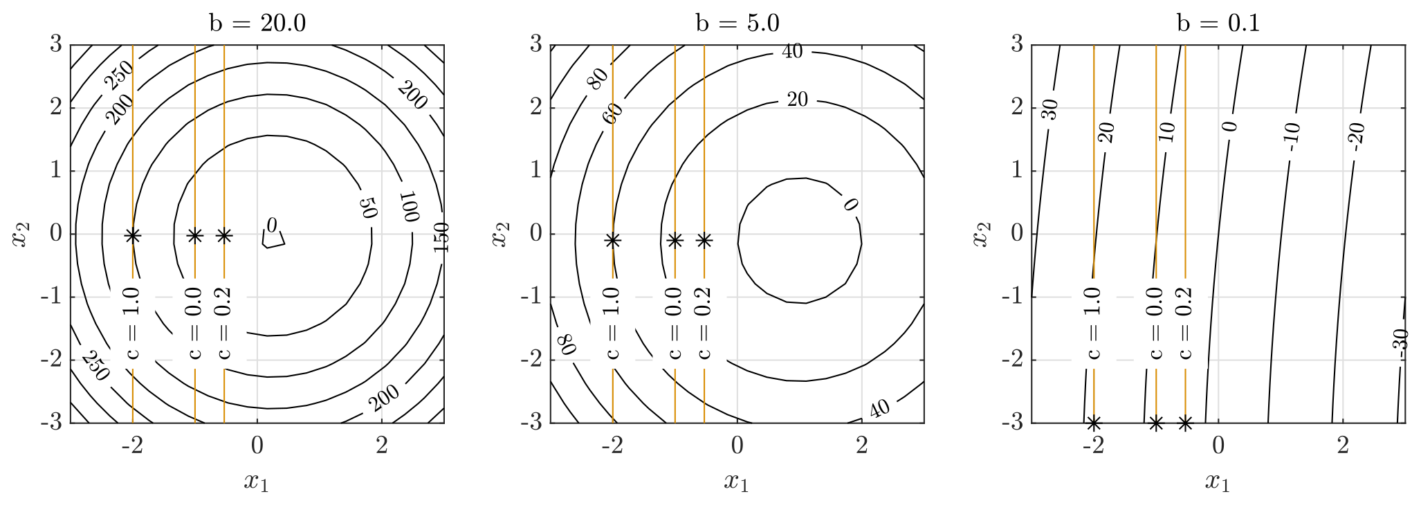
Figure C1 Contour plot of the objective function with the optimal value marked with an asterisk (^*), for objective functions with varying degrees of non-linearity in x. The higher the value of b, the more dominant the non-linear terms compared to the linear terms in the objective function. The constraint is represented as a yellow line and varies with c.

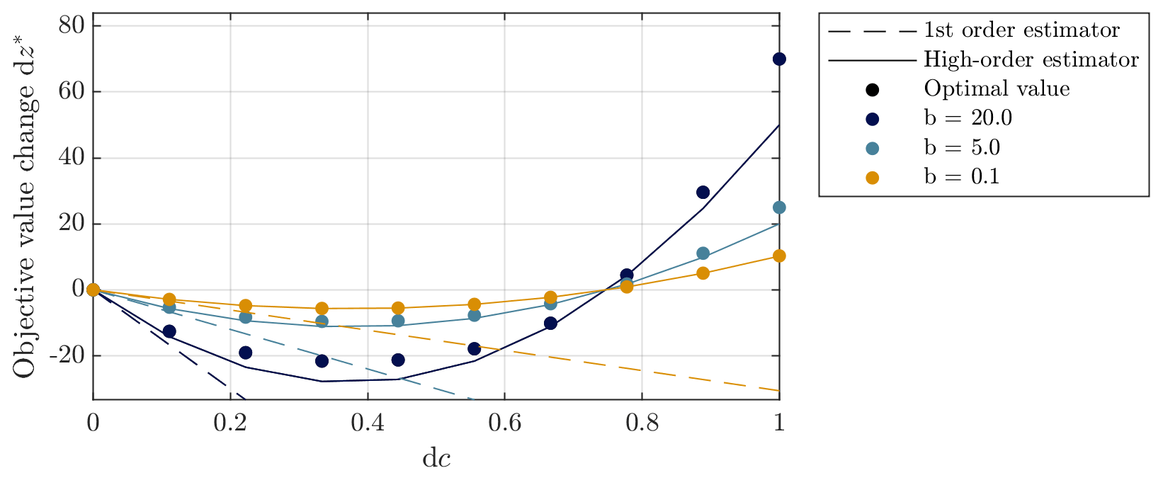
Figure C2 Comparison of the optimal objective value with the first-order estimator and the high-order estimator for objective functions with varying degrees of non-linearity in x. The higher the value of b, the more dominant the non-linear terms compared to the linear terms in the objective function.

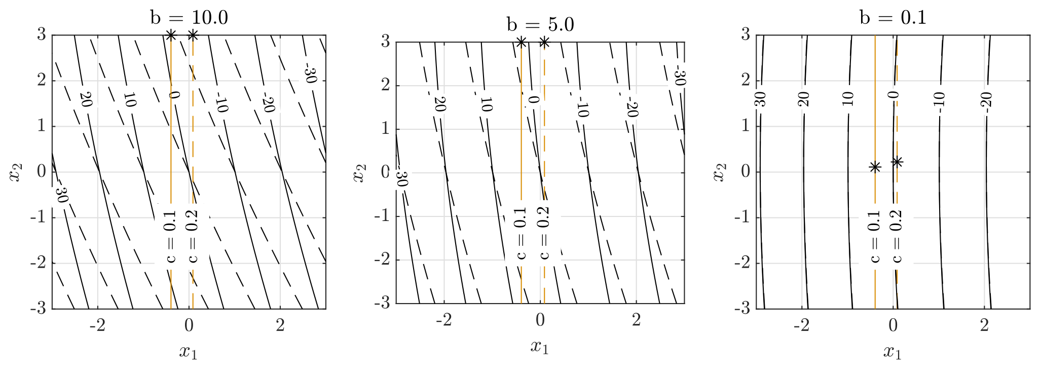
Figure C3 Contour plot of the objective function with the optimal value marked with an asterisk (^*), for problems with varying degrees of coupling between x and c in the objective function. The higher the value of b, the more dominant the coupling terms compared to the linear terms in the objective function. Results are represented with a solid line for c=0.1 and with a dashed line for c=0.2 in order to highlight the magnitude of the coupling between x and c.

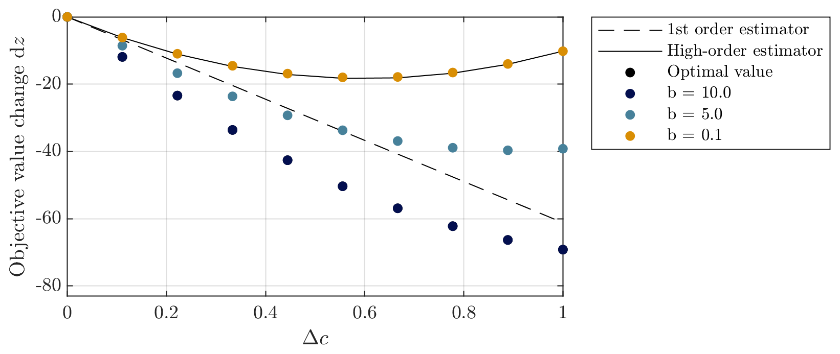
Figure C4 Comparison of the optimal objective value with the first-order estimator and the high-order estimator, for problems with varying degrees of coupling between x and c in the objective function. The higher the value of b, the more dominant the coupling terms compared to the linear terms in the objective function. The high-order estimator assumes b=0.

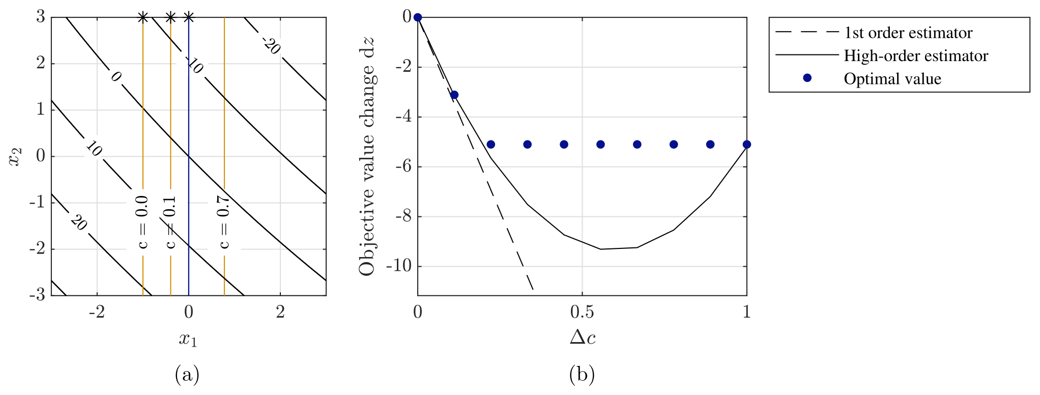
Figure C5 Contour plot of the objective function with the optimal value marked with an asterisk (^*), where the blue line represents the constraint non-dependent on c (a). Comparison between the first-order estimator, the high-order estimator, and the optimal objective value for variations in c (b).