the Creative Commons Attribution 4.0 License.
the Creative Commons Attribution 4.0 License.
 | 09 Jul 2024
Synchronised WindScanner field measurements of the induction zone between two closely spaced wind turbines
Anantha Padmanabhan Kidambi Sekar
Paul Hulsman
Marijn Floris van Dooren
Martin Kühn
Field measurements of the flow interaction between the near wake of an upstream wind turbine and the induction zone of a downstream turbine are scarce. Measuring and characterising these flow features in wind farms under various operational states can be used to evaluate numerical flow models and design of control systems. In this paper, we present induction zone measurements of a utility-scale 3.5 MW turbine with a rotor diameter of 126 m in a two-turbine wind farm operating under waked and unwaked conditions. The measurements were acquired by two synchronised continuous-wave WindScanner lidars that could resolve longitudinal and lateral velocities by dual-Doppler reconstruction. An error analysis was performed to quantify the uncertainty in measuring complex flow situations with two WindScanners. This is done by performing a large-eddy simulation while using the same measurement layout, modelling the WindScanner sensing characteristics and simulating similar inflow conditions observed in the field. The flow evolution in the induction zone of the downstream turbine was characterised by performing horizontal-plane dual-Doppler scans at hub height. The measurements were conducted for undisturbed, fully waked and partially waked flows. Evaluation of the engineering models of the undisturbed induction zone showed good agreement along the rotor axis. In the full-wake case, the measurements indicated a deceleration of the upstream turbine wake due to the downstream turbine induction zone as a result of the very short turbine spacing. During a wake steering experiment, the interaction between the laterally deflected wake of the upstream turbine and the induction zone of the downstream turbine could be measured for the first time in the field. Additionally, the analyses highlight the affiliated challenges while conducting field measurements with synchronised lidars.
- Article
(6293 KB) - Full-text XML
- BibTeX
- EndNote


During operation, wind turbines create a reduced-velocity region upstream due to rotor thrust, i.e. the induction zone. To account for the induction zone, the IEC 61400-12-1 (International Electrotechnical Commission, 2022) standard recommends performing freestream velocity measurements more than 2 to 4 rotor diameters (D) upstream of the turbine. Wind turbines also create wakes, the main driver of unfavourable aerodynamic interactions in a wind farm where the downstream turbine extracts less power and is subject to higher structural loads due to reduced wind speeds and high wake turbulence. The near wake of a turbine extends 2.0D to 4.0D downstream and is highly influenced by rotor aerodynamics (Göçmen et al., 2016). Therefore, for tightly packed wind farms, the induction zone of a downstream turbine can overlap with the near wake of an upstream turbine.
The upstream induction zone of a wind turbine has consequences for many wind power applications. The velocity deficit upstream of the turbine is responsible for the estimation bias in power curve measurements for isolated turbines (Slinger et al., 2020) and global blockage at the wind farm level (Schneemann et al., 2021). Moreover, the flow slowdown and expansion around the turbine also affect lidar-based feed-forward controllers, which require precise information on the velocity magnitudes and arrival times at the rotor (Dunne et al., 2014). Several approaches have previously been followed to numerically (Medici et al., 2011; Branlard and Gaunaa, 2015; Troldborg and Meyer Forsting, 2017) and experimentally (Asimakopoulos et al., 2014; Simley et al., 2016; Mikkelsen et al., 2020) investigate the induction zone in free inflow conditions. The most detailed three-dimensional triple-synchronised lidar characterisation of the induction zone by Simley et al. (2016) was performed around a Vestas V27 turbine with a diameter of 27 m, which is not representative of modern utility-scale multi-megawatt turbines.
Wind turbines operating in the downstream rows of wind farms are not always exposed to undisturbed inflow. Depending on the farm layout, wind direction, and wake effects such as meandering (Trujillo et al., 2011) and wake deflection strategies (Jiménez et al., 2009), the downstream turbines operate under partial or fully waked inflow. High-resolution measurements of the induction zone in partial and fully waked inflows are still limited.
Engineering models of the induction zone have been developed to accurately estimate the annual energy yield and implement flow control strategies. Medici et al. (2011) presented a one-dimensional model for the induction zone using a vortex sheet method. Branlard and Gaunaa (2015) developed a two-dimensional induction zone model based on a vortex cylinder implementation. Troldborg and Meyer Forsting (2017) presented a self-similar analytical two-dimensional induction zone model. Branlard and Meyer Forsting (2020) coupled these models with the wind farm simulation tool FLOw Redirection and Induction in Steady State (FLORIS) (NREL, 2023) to provide flow estimations for wind farm control purposes. Although the coupling was evaluated against actuator disc simulations, a comparison with full-field data has not yet been performed because of the lack of high-quality field measurements.
Lidars are capable of measuring the velocity through the Doppler shift remotely and provide a way to measure the flow around wind turbines in the field (Werner and Streicher, 2005). Field measurement campaigns using scanning lidars provide valuable data which can be used to characterise the induction zone behaviour for highly dynamic inflow conditions, atmospheric stabilities and turbine interactions. However, conducting full-field measurements is challenging because of the complicated installation; highly dynamic inflow conditions; finite number of measurement sensors; and their associated limitations and uncertainties, which add complexity during post-processing. Multi-lidar systems such as WindScanners (Simley et al., 2016) can perform user-defined trajectories, whereby the laser beams are synchronised in space and time, enabling the resolution of two or three wind velocity components depending on the number of devices used. These devices have previously been used to map the induction zone (Simley et al., 2016), measure the flow around trees (Angelou et al., 2021), assess helicopter downwash (Sjöholm et al., 2014) and operate in the wind tunnel (van Dooren et al., 2017; Hulsman et al., 2022b; van Dooren et al., 2022). Depending on the orientation and scan pattern, detailed two- or three-dimensional flow retrievals are possible. However, a thorough error and uncertainty assessment is required before interpreting the measurements, owing to the lidar measurement principle and scanning limitations, such as the volume-averaging effect, assumptions on the vertical velocity for dual-Doppler reconstruction, scanning speeds, beam pointing and intersection accuracies.
Several studies have been conducted to estimate the measurement accuracy of scanning lidar retrievals. An uncertainty analysis presented by van Dooren et al. (2017, 2022) considered the lidar measurement uncertainty and the artificially added uncertainty in the dual-Doppler reconstruction for a two-lidar configuration. Giyanani et al. (2022) presented an uncertainty model to reconstruct a three-dimensional wind vector considering the probe volume and the pointing accuracy for a three-lidar configuration. Emulating lidar measurement properties in high-fidelity computational fluid dynamics simulations provides a high-quality reference for error assessment and uncertainty quantification. Such approaches have been utilised extensively to understand long-range, pulsed scanning lidar measurements and their limitations (Lundquist et al., 2015; Bromm et al., 2018; Rahlves et al., 2022; Robey and Lundquist, 2022). For continuous-wave systems, Kelley et al. (2018) and Debnath et al. (2019) used virtual lidar in a large-eddy simulation (LES) approach to evaluate the accuracy of retrieving horizontal wind speeds for turbine-mounted wake scanning lidars considering effects such as probe volume averaging and assumption of zero vertical velocity and atmospheric effects such as stability. Meyer Forsting et al. (2017) utilised a virtual lidar technique to understand the influence of measurement averaging on wake measurements. They reported that the differences between lidar and point measurements are the greatest at wake edges where the probe volume extends from the wake into the freestream, reaching up to 30 % at 1D downstream and up to 60 % at 3D downstream.
In this study, two synchronised ground-based continuous-wave WindScanner lidars were used to characterise the flow region between two 3.5 MW turbines, which were spaced 2.7D apart. The very short spacing creates an interaction between the near wake of the upstream turbine and the induction zone of the downstream turbine. During the measurement campaign, we implemented an active wake steering control on the upstream turbine. The near-wake–induction zone interaction is of interest for wake steering control. Therefore, cases such as partial- and full-wake impingement with the induction zone are examined.
Considering the measurement campaign, the main objectives of the paper include the following:
-
demonstration of two-dimensional scanning of wind fields around utility-scale turbines with two synchronised WindScanner lidars;
-
identification and investigation of errors associated with performing ground-based synchronised scanning lidar measurements with two WindScanners in a controlled simulation environment;
-
characterisation of the two-dimensional induction zone behaviour and interaction between two closely spaced turbines for unwaked, waked and partially waked scenarios and evaluation of induction zone models.
The remainder of this paper is organised as follows. Section 2 describes the measurement and LES setup. The results from the LESs and the full-field measurements are discussed in Sect. 3. A discussion of the results and conclusions are presented in Sects. 4 and 5, respectively.
A description of the wind farm layout and the measurement setup is provided in Sect. 2.1. Section 2.2 contains information on the WindScanners, the programmed scan trajectories and the data processing methods. The collected datasets are presented in Sect. 2.4. The setup of the large-eddy simulation including the lidar simulator is explained in Sect. 2.5.
2.1 Test site description and inflow characterisation
The measurement campaign was conducted from November 2020 to June 2021 at a wind farm close to Kirch Mulsow in northern Germany. The site has two eno126 turbines from Eno Energy Systems GmbH with a rated wind speed of 11.4 m s−1 and power of 3.5 MW with a diameter D=126 m. The upstream and downstream turbines are abbreviated as WT1 and WT2, respectively.
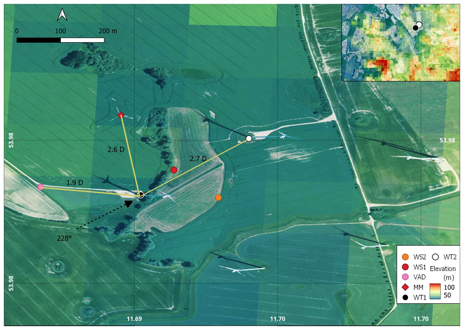
Figure 1The wind park and measurement layout at Kirch Mulsow, overlain with elevation contours. A zoomed-out image of the site is shown in the top-right corner, illustrating the hills present upstream of the wind park. MM and VAD refer to the met mast and the inflow lidar, while WS1 and WS2 refer to the two WindScanners. © Microsoft.
The layout of the site is illustrated in Fig. 1. The hub height of the downstream turbine at 137 m is 20 m higher than that of the upstream turbine at 117 m. The site itself is characterised as farmland with moderately rolling hills. The elevation data presented in Fig. 1 were obtained with a resolution of 200 m and are maintained by the German Federal Agency for Cartography and Geodesy. While the elevations at the turbine locations are approximately 52 m, abrupt changes in elevation are seen upstream, notably the presence of a small hill with an elevation of 105 m, 22D upstream of WT1 along the predominant wind direction of 228°. This creates a slope of 1.09° towards the two turbines. The village of Garvensdorf is approximately 1200 m (9.5D) upstream of WT1 along θwdir= 228°. Furthermore, a treeline exists between WT1 and WT2, extending towards the met mast with a height of approximately 15 to 20 m that can act as a windbreak and can cause perturbation to the wind flow (Counihan et al., 1974). Other treelines and clumps of forested areas are present at various upstream positions along θwdir= 228°. During the measurement campaign, wake steering tests were performed on WT1, leading to partial-wake scenarios at WT2. Additional information on the wake steering campaign is available in Hulsman et al. (2022a).
Inflow conditions were measured by a met mast placed 2.6D north of WT1, equipped with two anemometers, namely the Thies First Class Wind Transmitter anemometer of type 4.3352.00.400 at the lower tip of 54 m and close to the WT1 hub height of 116 m. The Thies First Class Wind Direction Transmitter wind vane of type 4.3151.00.212 is also installed at 112 m. All the instruments stored the data at a sampling rate of 50 Hz. To measure the atmospheric stability, an integrated open-path gas analyser and three-dimensional sonic anemometer (IRGASON, Campbell Scientific) were also installed on the mast at a height of 6 m on a boom oriented towards 136°. More details on the derivation of the Obukhov length from IRGASON are described in Bromm et al. (2018). The inflow measurements were further supported by a WindCube 200S lidar placed 1.9D upstream of the WT1. The ground-based lidar performed velocity azimuth display (VAD) scans with an elevation angle of 75° and with range gates set from 50 to 840 m with a spacing of 5 m and a pulse length of 25 m. The accumulation times and angular speeds were 0.5 s and 30° s−1, respectively. The data from the VAD scans were binned into 10 min averages from which the wind shear and veer profiles were estimated. The turbine heading of WT1 and WT2 during operation was measured precisely using a differential GPS of the Trimble Zephyr™ 3 model. All the measurement devices were synchronised to UTC time.
2.2 WindScanners
The WindScanners are continuous-wave (cw) scanning lidars with a steerable scanner head that users can programme to perform any user-defined scan trajectory (Mikkelsen et al., 2017). The steerable scanner head consists of two prisms connected to individual drives, which can be rotated independently, while a third motor is used to control the focal distance of the lidar. Each of the two prisms deflects the focused laser beam by ±30° to achieve a maximum measurement cone angle of 120°. In the present setup, the lidar can continuously sample line-of-sight speeds at a maximum sampling rate of 451.7 Hz. Two WindScanners were installed in the field in the region between the two turbines inside offshore containers for weather protection (Fig. 2a).
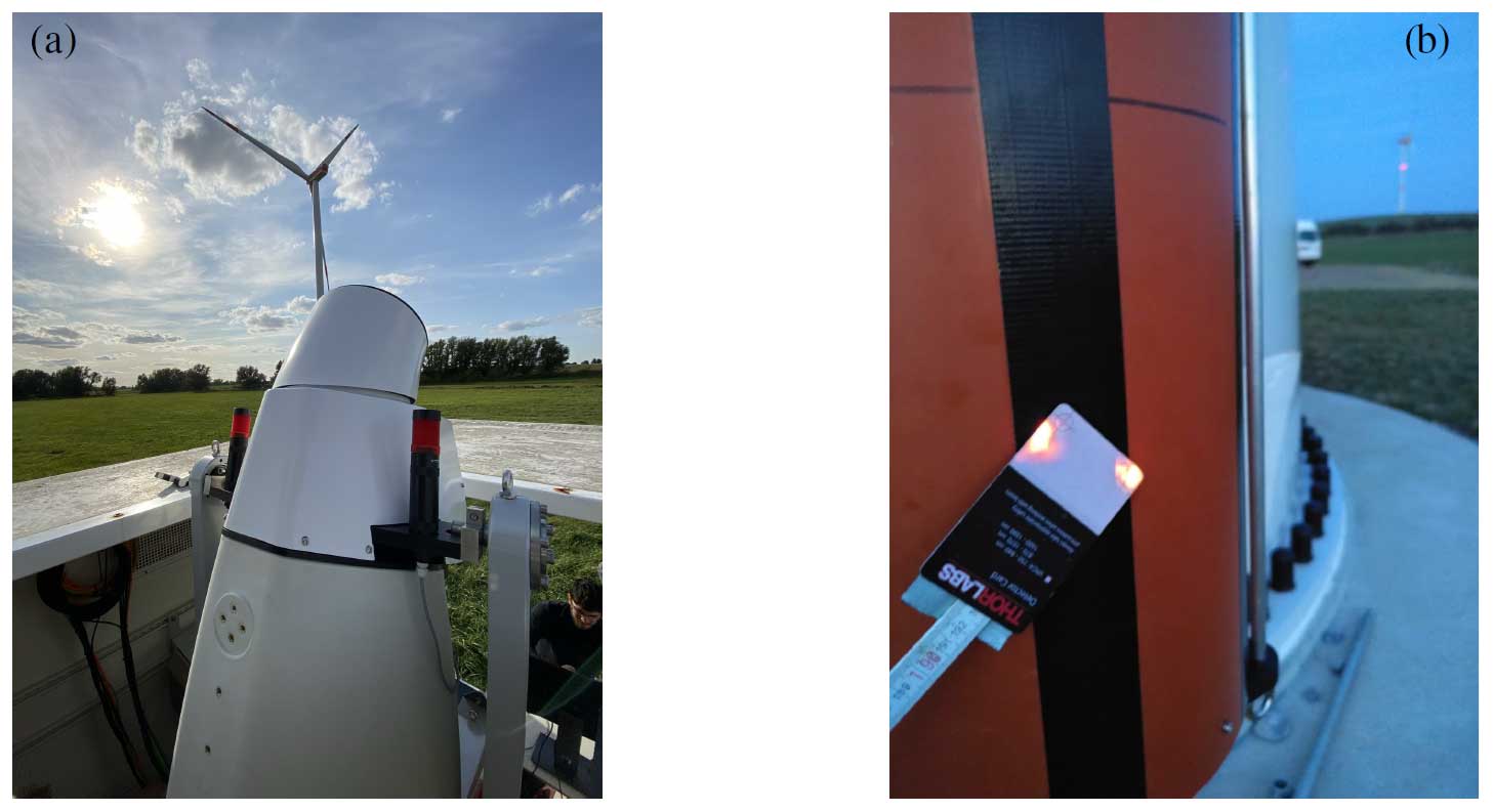
Figure 2(a) View of WS2 installed in a weatherproof container with WT1 in the background. The WindScanners were lifted through a hatch on the roof during operation using a hydraulic table. (b) The two laser beams from WS1 and WS2 simultaneously focused over a distance of approximately 200 m at WT2 onto a 5.3 cm × 8.6 cm laser beam detector card (white dots) after performing a steering calibration.
Both WindScanners synchronously provide a Doppler velocity spectrum for every measurement sample calculated from a discrete Fourier transform of the backscattered light sampled at 120 MHz. The individual Doppler spectra are averaged to reduce noise, and the shot-noise-based mean background spectrum is removed to obtain the peak of the Doppler spectra. The line-of-sight velocity is estimated by determining the spectral peak through the median peak-finding method for continuous-wave lidars, as it is less sensitive to spurious noise than the centroid and maximum methods (Angelou et al., 2012).
A single lidar can only estimate the line-of-sight (vlos) speed along the laser beam direction that contains contributions from all three velocity components:
where u, v and w are the longitudinal, lateral and vertical wind velocity components, respectively, and χ and δ are the azimuth and elevation of the laser beam, respectively. By synchronising the two WindScanners in time and space, the WindScanners can estimate the two-dimensional wind speed component projected on the plane and defined by the beams in the intersection point.
The u and v velocity components can be resolved by an additional assumption of the vertical flow component and combining the two vlos measurements by dual-Doppler wind field reconstruction by solving Eq. (2). Equation (2) can now be rewritten as
In our measurements, the actual local value of the w component is unknown. Without generalisation, we assume that the vertical flow component vanishes in our case. The uncertainty associated with measuring three-dimensional flow events with two synchronous lidars is discussed in Sect. 2.3. Another important lidar measurement property is volume averaging; that is, the vlos measurements contain weighted contributions along a volume extending on either side of the focus point along the laser beam direction. The measured line-of-sight velocities of a cw lidar at the position , vlos(x) can be mathematically expressed as the convolution of the wind vector u(x) projected along the laser beam direction and the volume-averaging function:
Here, n is the unit vector along the line-of-sight direction, and ϕ(s) is the spatial volume-averaging function following Sonnenschein and Horrigan (1971) for cw lidars approximated as a Lorentzian function, where s is the distance from the focal point along the laser beam. For cw lidars, the range weighting of line-of-sight speeds that occur along the laser beam direction at a point located at a distance f away from the lidar can be expressed as the full width at half maximum (FWHM) of the focused laser beam . Here, λ=1.56 µm and a=56 mm are the laser wavelength and effective radius of the lidar’s 6 in. (15.2 cm) aperture telescope, respectively. As the length of the measurement volume is related to f2, the measurement volume is quite large at large distances, and hence turbulent structures smaller than the measurement volume will be low-pass filtered by the lidar.
2.2.1 Scanning patterns
The region of interest within this work is the inflow of WT2. The WindScanners are programmed to perform spatially and temporally synchronised horizontal-plane scans upstream of WT2. The measurement plane is at hub height and centred around the alignment of WT1 and WT2 at 228°. The WindScanners were not perfectly symmetrical to WT2 because of a treeline that prohibited symmetrical placement of WS1 with WS2 and WT2. The measurements are visualised in a global fixed reference frame centred at the bottom of WT2, where the x axis is the connecting line between the two turbines, and the y and z axes are positive to the right looking towards WT2 and in an upward direction. The scan pattern was composed of a sinusoidal variation in the x and y coordinates of the focal point:
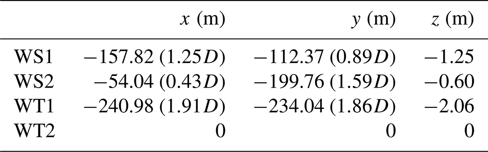
Here Ax= 0.60D and Ay= 0.59D are the amplitudes; , y0=0D and z0= 137.0 m are the offsets; and T is the time period to complete each trajectory, with each scan taking 29.6 s to complete. The horizontal-scan plane at the hub height of WT2 extends from 0.8D upstream of the turbine to 0.4D downstream, with a width of 1.18D, as shown in Fig. 3. The offsets due to the terrain-induced height differences and the vertical offset of the WindScanners inside the container mounting are included in Eq. (6) and are tabulated in Table 1.
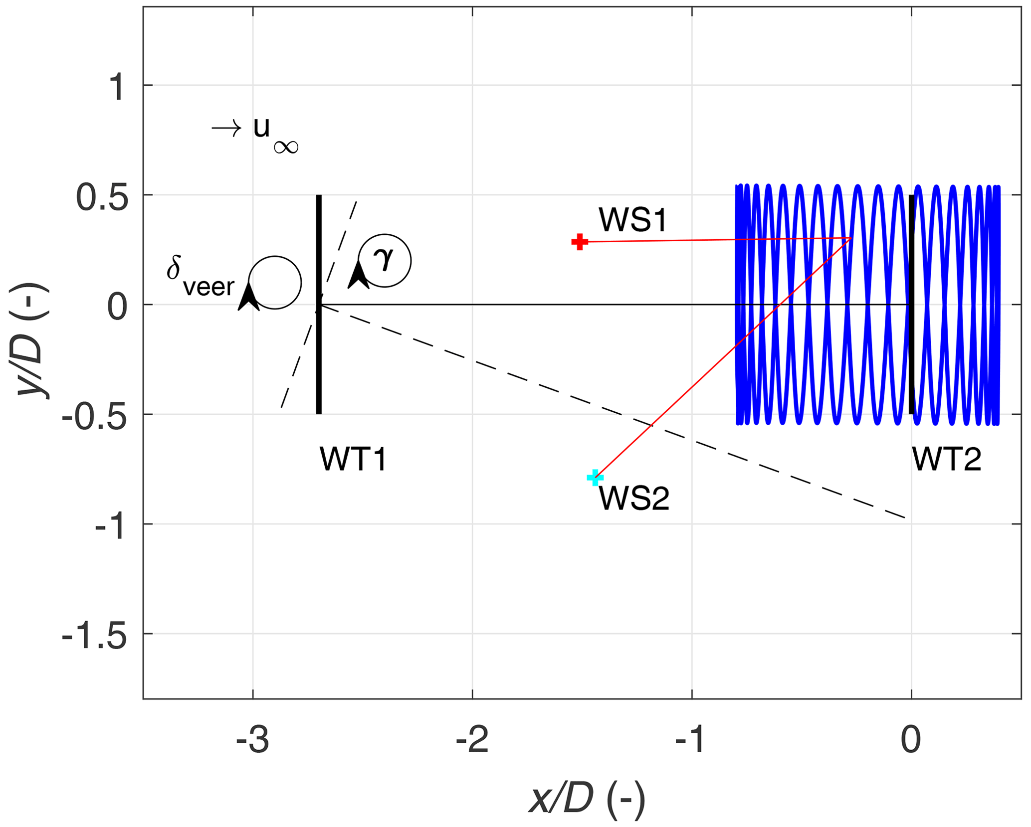
Figure 3Illustration of the horizontal scanning pattern performed by the WindScanners, indicating the relative position of the two turbines and the two WindScanners with and without an intentional misalignment. The coordinate system is centred at the bottom of WT2.
Table 1Relative and normalised distances from the bottom of WT2 and WS1, WS2 and WT1. The height offsets for WS1 and WS2 are calculated from the middle of the outer prism at the highest jacked-up position of the hydraulic table (Fig. 2a).
With a temporal sampling rate set at 451.7 Hz, each complete scan had approximately 13 079 measurement points. In this sector, active wake steering was performed by toggling between two unique wake steering controllers and one greedy controller where no wake steering is performed, each operational for 35 min. The measurement campaign regarding the active wake steering is described in detail in Hulsman et al. (2022a). The WindScanner measurements are then subdivided into 35 min blocks, each representing a different operating state of the upstream turbine. All horizontal-plane scans are grouped and averaged to obtain averaged profiles of the measured longitudinal and lateral velocities. For visualisation, the longitudinal and lateral velocities are interpolated onto a uniform grid with a spacing of 10 m using a cubic interpolation scheme. We rotated all measurements in the global reference frame into the main wind direction measured at the met mast at 1 m below WT1 hub height.
2.3 WindScanner measurement errors and uncertainties
While performing synchronised WindScanner measurements, several errors affecting the measurement accuracy can be broadly divided into single- and dual-lidar errors. For this particular site and measurement setup, the various lidar errors, their impact and their analysis methodology are tabulated in Table 2.
Table 2Summary of dual-Doppler lidar measurement errors. Here, LES and SUP refer to large-eddy simulation and standard uncertainty propagation methods that are described in the following sections.

2.3.1 Single-lidar errors and uncertainties
First, we discuss the sources of the errors associated with single-lidar systems. For WindScanners, the absolute measurement uncertainty in the lidar radial velocity estimation was experimentally determined by Pedersen and Courtney (2021) to be less than 0.1 % under nearly ideal conditions.
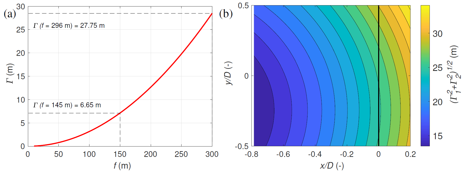
Figure 4(a) The variation in the lidar measurement volume with focus distance. The dashed lines indicate the minimum and maximum measurement ranges. (b) The variation in the effective lidar measurement volume within the scanning area.
While performing scanning cw lidar measurements, a variable measurement volume exists throughout the scan area. For the horizontal scans, the WindScanners measured at distances from 145 to 296 m, corresponding to a probe volume ranging from 6.65 m (0.05D) to 27.75 m (0.21D), as shown in Fig. 4a, b. The WindScanners, with their larger 6 in. (15.2 cm) aperture and shorter focus rods, enabled the probe volume to remain below 30 m (0.24D) even at the maximum 300 m range in comparison to the previously used 3 in. (7.6 cm) WindScanners with smaller apertures (van Dooren et al., 2017). The probe volume-averaging effect is a significant source of uncertainty, especially at considerable focus distances, as it can lead to a measured wind speed bias in a sheared flow. This effect concerns our study as it is most severe for measurements at the wake edges, as the measurement volume extends from inside the wake to the freestream, and for measurements very close to the downstream turbine WT2, as the measurement volume would extend partially into the turbine wake. Due to range weighting, velocity measurements are subject to spatial filtering that attenuates the high-frequency wind information, which makes estimates of small-scale turbulence challenging at large focal distances.
2.3.2 Dual-lidar errors and uncertainties
Next, we discuss dual-Doppler pointing accuracy, which concerns the ability to steer the focused laser beam to a predefined point in space. To enable dual-Doppler wind field reconstruction, the laser beams from the two WindScanners must focus and be spatially and temporally synchronised with each other. The scanner orientation and levelling were thoroughly checked in a controlled laboratory. The final calibration of the steering motors was performed using the turbine tower and a rotating setup as hard targets and by locating the laser beams using an infrared sensor card (Fig. 2b). A pointing accuracy of 0.1° was determined in the field from the commanded and actual positions of the motors steering the prism. The temporal synchronisation of WindScanners was validated in a previous wind tunnel campaign by van Dooren et al. (2022) and in the field by Giyanani et al. (2022). Giyanani et al. (2022) also estimated similar ranges for the pointing accuracy and calculated the effective intersection diameter at the intersection volume of laser beams to be of the order of 2 to 5 m.
Due to the spatial and temporal variation in turbulence and the scanning strategy that requires a finite amount of time to complete each scan, the dominant flow features in the induction zone would not be revealed until multiple scans are collected and averaged. The chosen averaging period must allow the mean velocity measurements to converge while maintaining similar flow conditions throughout the scan duration. Simley et al. (2016) showed that for their measurements where each longitudinal scan took 10 s to complete, the dominant flow features were revealed after averaging for at least 3 min (18 scans), while the results were presented as 10 min (60 scans) averages. In our setup, owing to the active toggling of the yaw controller on WT1, the inflow into WT2 changed every 35 min; hence, a maximum of only 71 complete scans was available for ensemble averaging over 35 min. The ability of WindScanners to capture salient flow features in the induction zone is further investigated in Sect. 3.1 through statistical uncertainty analysis.
The error in the dual-Doppler reconstruction is dependent on the relative alignment Rint of the laser beams to each other, which depends on the lidar position and measurement trajectory (Stawiarski et al., 2013; Peña and Mann, 2019). If the two laser beams are aligned with each other and with the main wind direction, the longitudinal wind component can be estimated accurately, whereas the orthogonal wind speed component cannot be accurately reconstructed. In other words, when the intersection angle tends towards 0 or 180°, the lateral component cannot be resolved. Figure 5a illustrates the variation in Rint in the scan plane, which decreases from 68° at to 34° at .
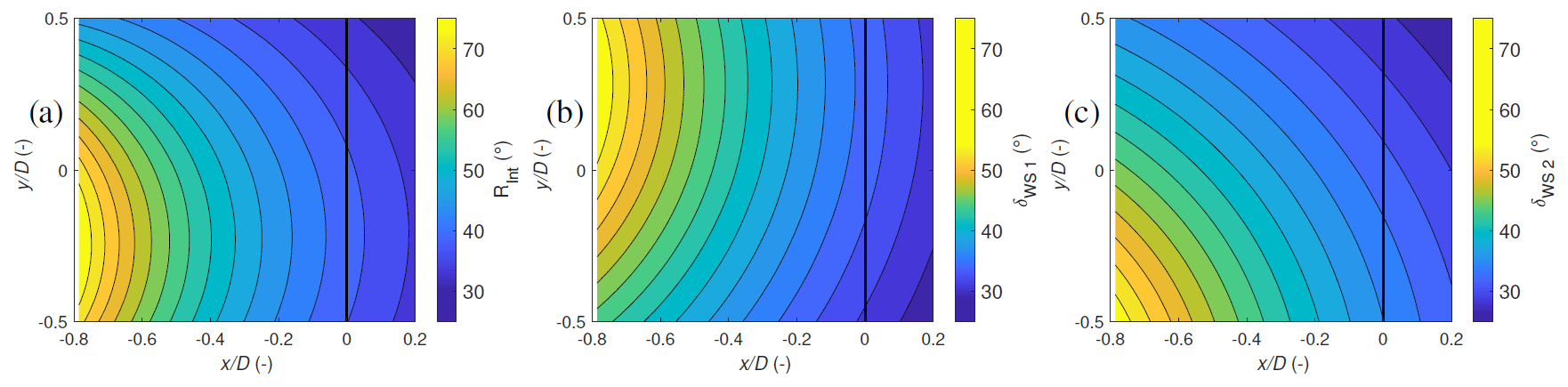
Figure 5The variation in the beam intersection angle Rint (a) and the elevation angles δWS1 (b) and δWS2 (c) in the scanning area. WT2 is represented by the black vertical line at 0.
The rotation in the wake of the upstream turbine induces a non-negligible vertical component in the flow. Therefore, the w=0 m s−1 assumption to obtain Eq. (2) contributes to an error in dual-Doppler reconstruction. As the WindScanners are programmed to scan at the WT2 hub height (137 m), the corresponding elevation angles for WS1 (28 to 55°) and WS2 (25 to 56°) introduce a directional bias (Fig. 5b, c). Hence in Eq. (1), the spatial variation in the non-zero vertical component and the corresponding sin (δ) terms are a major error source, especially at measurement points with large elevation angles. While installing the lidars closer to WT1 would reduce the required elevation angles, the lidar position was dictated and limited by the maximum achievable 300 m of range and available installation area.
Furthermore, we calculate the total uncertainty in the estimation of the longitudinal (eu) and lateral (ev) wind components by applying the standard uncertainty propagation (SUP) method (Stawiarski et al., 2013; van Dooren et al., 2017) on Eqs. (3) and (4). Assuming small errors and zero correlation between them, the method considers the total propagated uncertainty in the dual-Doppler reconstruction due to beam intersection angles, pointing errors and line-of-sight estimation errors due to neglecting the vertical flow component and is described by the following equations:
where and are line-of-sight errors; ew is the error due to the assumption of zero vertical velocity, i.e. the true value of w; and and are lidar pointing errors. All the uncertainty terms in the paper are the 1.96σ values of the corresponding error distributions; i.e. they are expected to include 95 % of all values. While SUP can be used to understand the influence of different aspects concerning measurement accuracy, not all errors can be studied in detail due to lack of references. Therefore, we also used additional lidar simulations to understand and quantify the different errors affecting the dual-Doppler reconstruction. The impact of the measurement volume, averaging times, lidar placement and trajectory on the measurements is qualitatively investigated in Sect. 3.1 using a virtual lidar within LES.
2.4 Measurements
As the region of interest was the zone between the two turbines, measurements were only performed when the turbines were aligned, i.e. when the wind direction was approximately 228°. We noticed that many measurements were also affected by unfavourable conditions, such as rainfall and lower availability of aerosols to backscatter the laser beam. For operational safety reasons, the WindScanners were operated only with on-site personnel supervision. The measurements were further influenced due to the presence of the wind turbine nacelle and the rotating blades that would systematically reduce data availabilities in the scan region. We present exemplary measurements of four cases made during February 2021, which are summarised and tabulated in Table 3.
Table 3Overview of the measurement cases acquired in the field. Each case is characterised by its freestream wind speed u∞, turbulence intensity (TI), integral length scale (Ti), mean θwdir and its standard deviation within the measurement period, stability parameter (), stability, wind veer (γ), αshear, and the yaw offset of the turbines (γWT). Here the following abbreviations are used: strongly stable (SS), weakly stable (WS) and near neutral (NN).
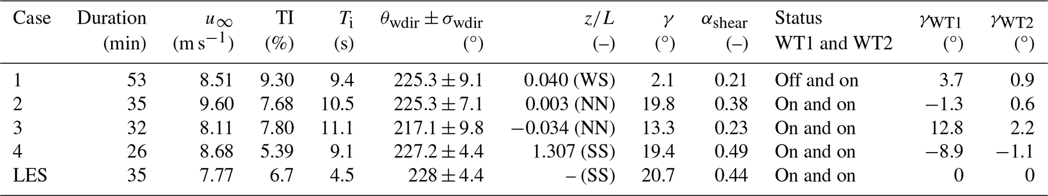
In Case 1, WT1 was switched off, while WT2 was operational; hence, an undisturbed induction zone upstream of WT2 was expected. In Case 2, the two turbines were active and aligned, creating a full-wake inflow scenario for WT2. Cases 3 and 4 are measurements conducted while the wake steering control was active on the upstream turbine with averaged measured yaw offsets of 12.8 and −8.9°, respectively, creating a partial-wake scenario at WT2.
The freestream wind speed u∞, turbulence intensity TI, wind direction θwdir and its standard deviation were calculated using the anemometer and wind vane at the hub height of WT1 placed on the met mast. The integral timescales Ti are calculated following Cheynet et al. (2016) by integrating the auto-correlation function until the first zero crossing. The atmospheric stability of the boundary layer can be characterised well by the Monin–Obukhov similarity theory (Monin and Obukhov, 1954; Barthelmie, 1999). The Obukhov parameter () was measured by the eddy covariance station at a height of 6 m above the ground. The Monin–Obukhov length was calculated as
where u* denotes the friction velocity, k=0.4 denotes the von Kármán constant, g denotes the acceleration due to gravity, θs denotes the sonic temperature and denotes the buoyancy flux. The friction velocity is estimated as . The stability classification of the Obukhov parameter is performed for 30 min averages based on Wyngaard (2010) and further used in Simley et al. (2016), where negative values indicate the presence of unstable conditions (), positive values () correspond to stable conditions and values close to zero () are related to neutral conditions.
The wind shear profile was also estimated from the VAD lidar by fitting a shear exponent αshear based on the power law between the top and bottom blade tips. The test site experienced larger-than-expected values of wind shear with an average value of 0.3 throughout the measurement campaign (Sengers et al., 2023). The wind veer γ was calculated from the VAD lidar as the difference in wind direction between the top and bottom blade tips and was clockwise positive. The actual yaw offset γWT was calculated by subtracting the GPS-measured WT1 heading from the wind direction at the hub height measured from the met mast as follows:
A positive yaw misalignment was identified when the turbine was rotated clockwise when viewed from the top (Fig. 3). Data filtering for the field measurements was performed using a kernel-density-based filter based on Beck and Kühn (2017) to identify and remove low-quality measurements. The method filters for the line-of-sight velocity and the signal-to-noise-ratio (SNR) in a bi-variate manner based upon the assumption of self-similarity of valid data. The method is applied on all the collected vvlos measurements on the measurement plane and is capable of identifying hard targets, such as the nacelle and blades, through the clusters in the vvlos SNR space. The measurements are discretised and grouped into bins based on their vvlos SNR values. The frequency distribution of data points within each bin was then determined. Bins with frequencies exceeding 20 % of the most populated bin were retained for further analysis.
2.5 Numerical simulations of the experimental site
Before interpreting results, it is necessary to quantify the effect of the lidar measurement error and uncertainties discussed in Sect. 2.3. To this end, we modelled the wind farm and inflow conditions in a simulation environment. The wind data are obtained from high-fidelity LES runs where the performance of two virtual WindScanners was assessed. The wind field was created using high-resolution LES performed with the Parallelized Large-Eddy Simulation Model (PALM). The PALM code is widely used for atmospheric boundary layer studies and works by solving the filtered, incompressible, non-hydrostatic Navier–Stokes equations. Further details of the model are available in Maronga et al. (2015). A single stably stratified LES run was performed, and the two eno126 turbines were simulated with the actuator sector method using the Fatigue, Aerodynamics, Structures, and Turbulence (FAST) v8 code (Jonkman and Buhl, 2005) of the National Renewable Energy Laboratory (NREL), which is directly coupled with the LES (Krüger et al., 2022), allowing for the transfer of forces and velocities between the two simulations. The turbine FAST model was built using the aerodynamic properties, tower properties and turbine controller provided by the farm operator. The eigenfrequencies of the FAST model of the two turbines are further tuned based on load data measured during the experiments. The WindScanners were simulated using the integrated lidar simulator (LiXim) developed by Trabucchi (2020), which can simulate lidar kinematic and optical properties. LiXim simulates the volume-averaging property by discretising Eq. (5) in the LES, while the uncertainty in beam pointing and environmental factors is not modelled.
An atmospheric boundary layer of stable stratification was simulated in a domain of dimensions with a uniform grid spacing of 5 m. Turbulence recycling (Lund et al., 1998) was applied at a distance of 15D from the inlet, where the instantaneous wind fields of the precursor simulation are introduced into the main simulation. The potential temperature at the ground was set to 280 K. A potential temperature gradient of 1 K per 100 m was prescribed from 100 m above the ground, while the simulation was performed for 4800 s sampled at 5 Hz. For the analysis, the first 600 s of the simulation was removed to avoid transient effects, and only the final 35 simulation minutes was utilised to correspond with the field measurements. The terrain was modelled by prescribing a ground roughness length of 0.1 m. The simulated wind field has a mean wind speed at hub height u∞=7.77 m s−1 and a TI = 6.7 %. The stable atmospheric boundary layer (ABL) is characterised by a strong shear exponent αshear=0.44 and a wind veer of 20.7° between the top and bottom rotor tips. The virtual WindScanners are programmed to perform horizontal-plane scans similar to the experimental setup following Eq. (6). The two operational turbines aligned in the prevailing wind direction in the LES resembled a full-wake scenario at WT2.
This section is divided into two parts. In the first section, we show the results of the virtual WindScanner simulations in the LES and estimate the uncertainty associated with the dual-Doppler reconstruction. The results from the field measurements are presented in the second section. As the measurement plane extends 0.4D downstream of WT2, laser beam blockage due to blade rotation was expected. During post-processing, it was discovered that the data quality for the measurements at was poor, and the data were hence discarded for both LES and field measurements. A comparison against engineering models of the induction zone is shown only for the undisturbed induction case.
3.1 Virtual WindScanner evaluation in LES
Line-of-sight simulations of the two WindScanners are performed using LiXim and the LES flow field, after which a dual-Doppler reconstruction is applied to resolve the longitudinal and lateral wind fields. In Fig. 6, reconstructions of the WindScanner-estimated 35 min averaged longitudinal and lateral wind profiles are presented alongside the reference LES. Good qualitative agreement between the LES and the virtual WindScanner-resolved u and v profiles is noted at most parts of the scanning area. The simulations reveal that the WindScanners can capture the spatial features in the flow, such as the wake rotation and flow expansion at the rotor tips. For the u profiles, the velocity profiles show deviations from the LES reference, presumably because of the directional bias induced by the large elevation angles and the probe volume extending through the shear layer and from the wake into the freestream. The lateral velocity profiles illustrating the wake rotation and flow expansion are captured well by the WindScanners. The profiles also indicate that the dominant flow structures in the induction zone are captured well for an average duration of 35 min when similar wind conditions are maintained for the scan duration.
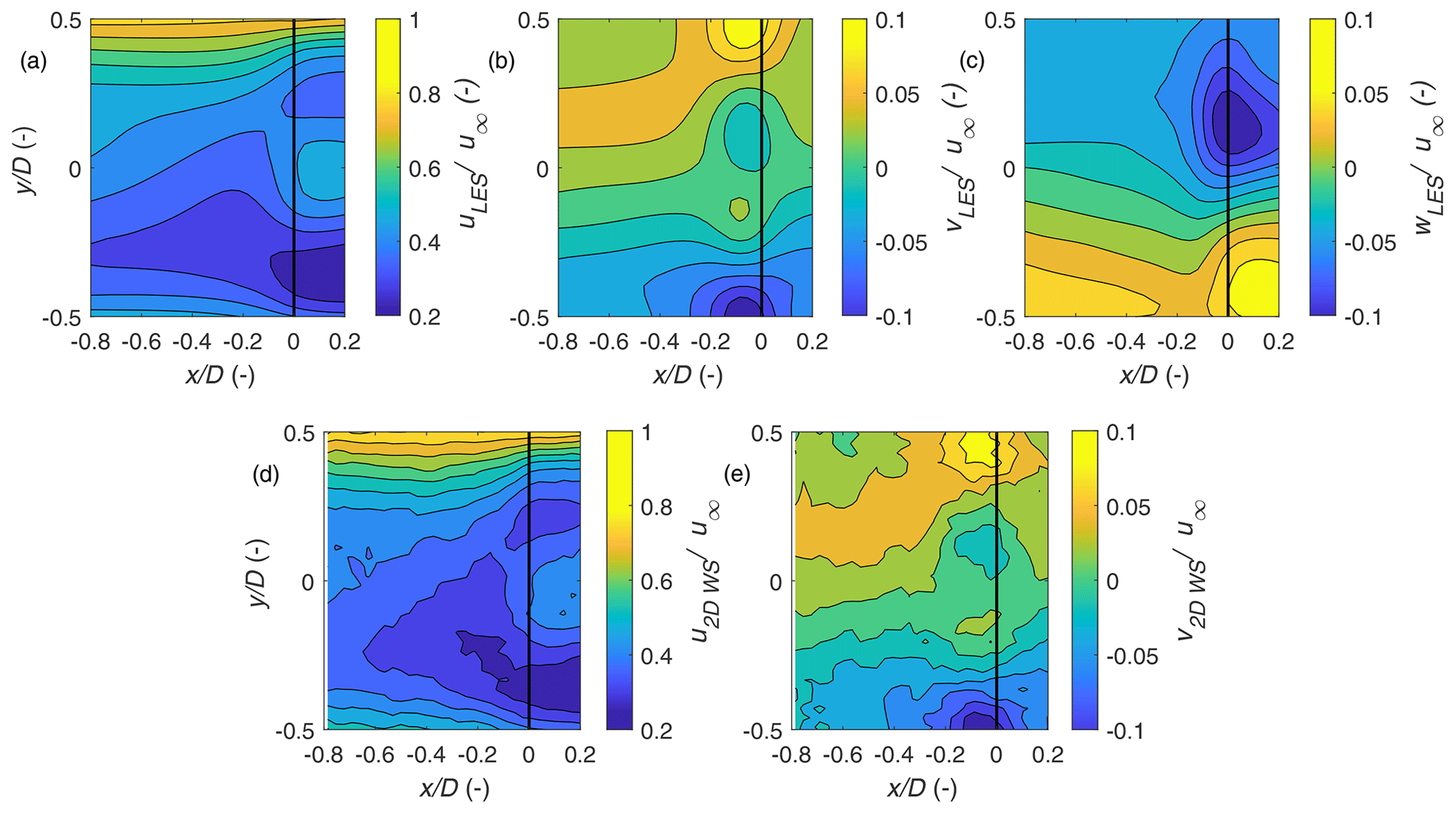
Figure 6Longitudinal (u), lateral (v) and vertical (w) velocities on the horizontal plane from the LES (a, b, c) and the results of the two-dimensional WindScanner reconstruction inside the LES (d, e), both averaged for the last 35 min of the simulation. The black vertical line at is the rotor of WT2.
3.1.1 Statistical uncertainty
First, we discuss statistical uncertainty denoting the standard error of the mean. While the total propagated uncertainty considers the propagation of uncertainty of single variables through the dual-Doppler reconstruction, the statistical uncertainty quantifies the precision of the results from different scans, with a higher number of scans typically reducing measurement noise from the statistical error. To quantify the statistical uncertainty, we use the margin of error estimated in the scanning area. It was calculated as and . Here, zγ, the confidence level, is set to 1.96, denoting the 95 % confidence interval; σu and σv are the standard deviations of the longitudinal and lateral velocity components in the scan plane obtained from the WindScanner simulations; and N is the number of samples.
Application of these equations to calculate the statistical error requires a large number of uncorrelated samples. Therefore, the independence of the measurement samples is analysed by checking if the scanning time is long enough to ensure that the samples are separated by several multiples of integral length scales (Table 3). According to Tennekes and Lumley (2018), for statistical independence, sampling the wind once every two integral timescales is adequate. For our investigated cases, the scan time multiples of the integral length scale vary from 2.6 to 6.5. Therefore, while the measurements may not be entirely independent due to the relatively short integral timescale compared to the scanning time, they may still be treated as approximately independent.
We now calculate the statistical uncertainty using to estimate the statistical uncertainty, where Ns is the number of independent samples. This effective sample size accounts for correlations in the turbulent flow, leading to a more accurate estimate of the error of the mean. The effective sample size is calculated based on Wilks (2019) as
where r is the lag-1 auto-correlation.
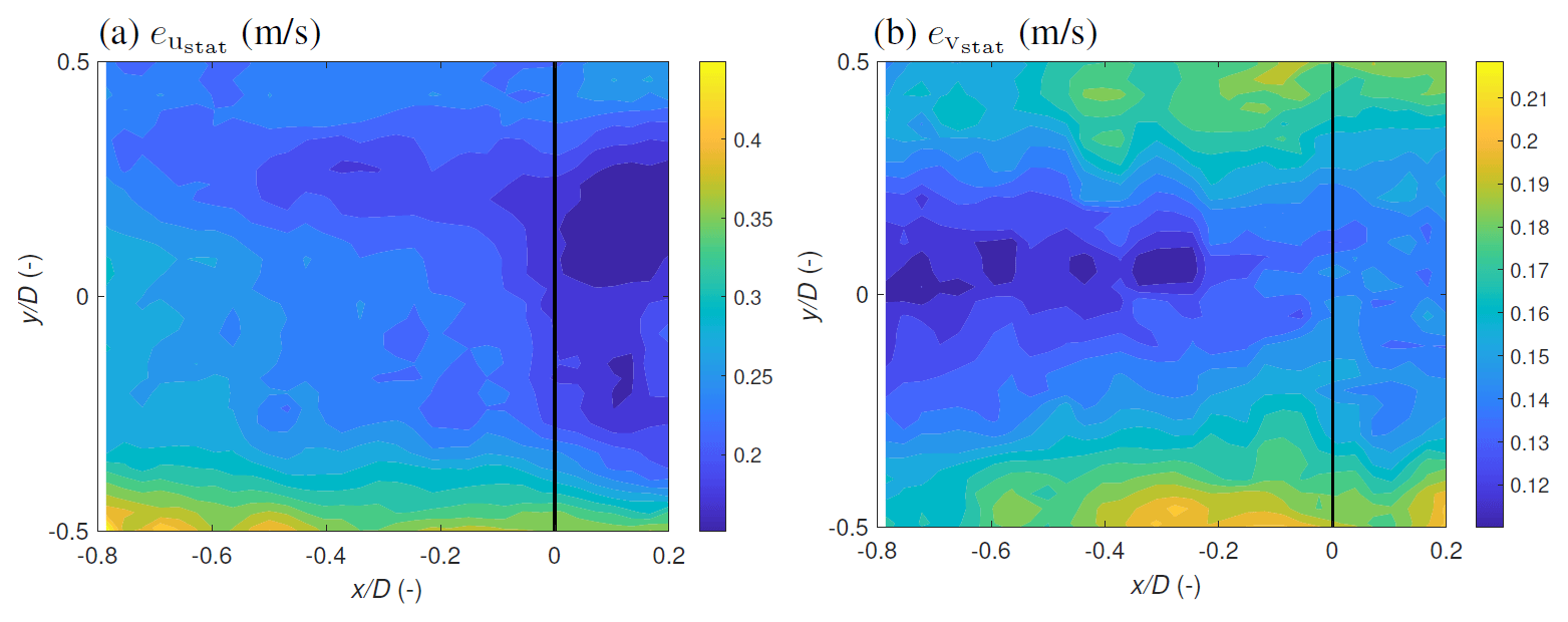
Figure 7Statistical uncertainty estimated through the margin of error for the (a) u and (b) v components for the evaluated LES flow field.
Figure 7 shows the variation in the margin of error in the scanning area for the two reconstructed components. The margin of error for the longitudinal component varies in the scan area between 0.2 and 0.4 m s−1 depending on the turbulence intensity in the wake. Similarly, for the v component, the margin of error varies up to 0.21 m s−1. The higher errors at scan edges could be attributed to the low number of data points in these locations as a consequence of the scanning patterns. In the field, we expect that the margin of error would be slightly higher than in the idealised LES due to the filtering procedure reducing data availability in each scan.
3.1.2 Dual-Doppler propagated uncertainty in LES
Secondly, we discuss the total propagated uncertainties estimated through the SUP method. The total propagated errors in the estimation of the longitudinal and lateral wind speed components are performed based on Eqs. (7) and (8) and illustrated in Fig. 8. To study the influence of spatial velocity variation in the wake, the actual LES w component in Fig. 6 is used. The u-component estimation error eu varied between 0.2 and 1 m s−1. As expected, eu is large at the WT2 rotor plane for the locations exhibiting higher w velocities. eu is the highest at the scan location closest to WS1, which has the highest elevation angles, where the lidars could only measure a small projection of the longitudinal wind speed. Similar behaviour is seen for ev as well, ranging from 0.4 to 1.1 m s−1 in the scanning area, with the highest values seen where larger w velocities are present and at the scan area where the beam intersection angles are the lowest (Fig. 5).
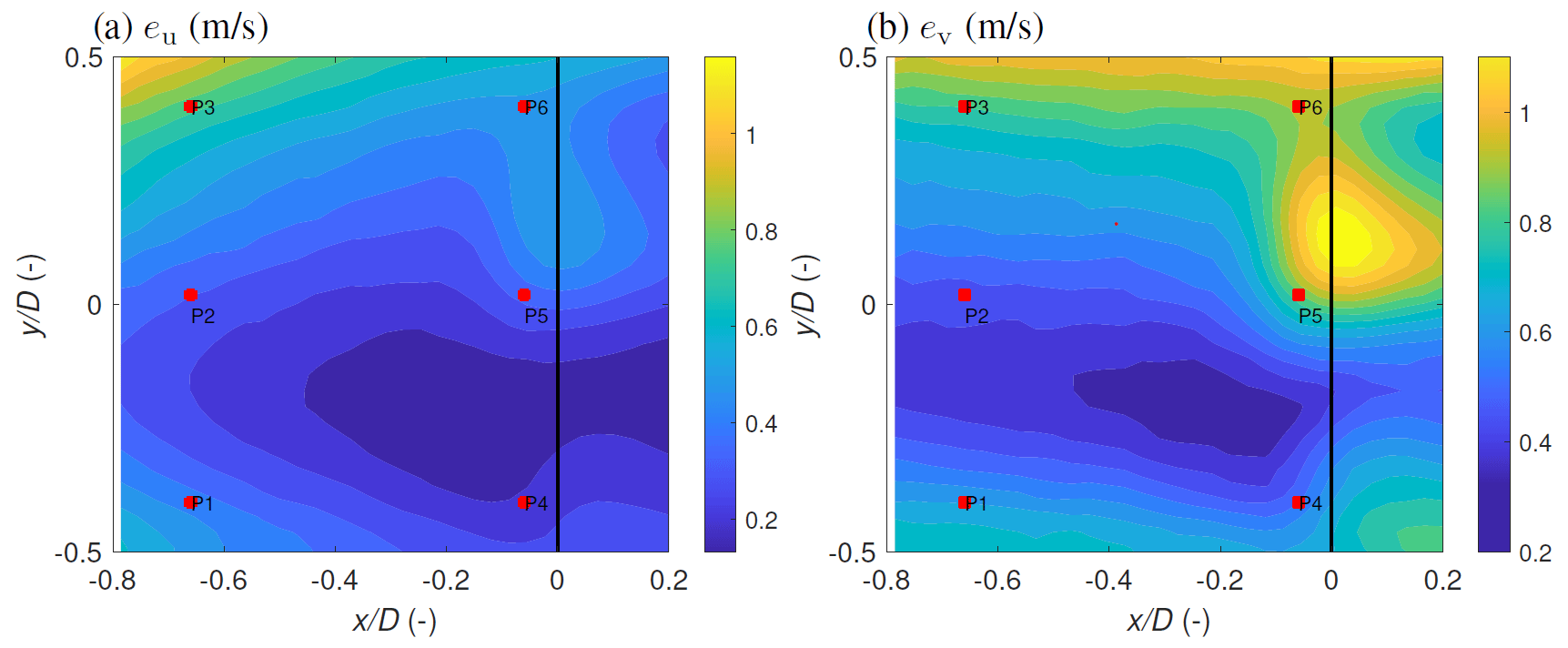
Figure 8Dual-Doppler reconstruction error for (a) the longitudinal (eu) and (b) the lateral (ev) components for the evaluated LES flow field. The markers P1–P6 indicate regions of interest.
Figure 9 illustrates the quadratic contributions of the different error terms in Eqs. (7) and (8) and the total error for the respective flow component visualised for six locations (P1, P2, … , P6) as marked in Fig. 8. To analyse the contribution of certain measurement errors, the standard uncertainty propagation is evaluated for an error in vlos of 0.1 %, a pointing accuracy of 0.1°, while the error introduced due to neglecting the vertical flow component is obtained from the local LES w component. The magnitude of the individual error contributions is normalised by the total error (eu, ev) to obtain the contribution of each term to the total error. For eu, the following trends are noticed. The contribution of the line-of-sight error evlos,i is almost negligible for all six points. The error due to the w-component assumption ew,i contributes significantly to eu, especially at P4, P5 and P6 due to the large local w at these locations. At P1, P2 and P3, has a large contribution due to the severe elevation angles required to scan at these points and the positive correlation between and δ. The varying contributions of ew,i at the points of interest can be explained by the relative alignment of the lidar with the wind direction. For a non-zero w component, an aligned lidar will contain a larger contribution of the w component projected onto its line of sight compared to the unaligned case. At P1 and P4, the contribution of ew,2 is the largest as WS2 is more aligned with the longitudinal wind component in comparison to WS1. Similarly, at P3, P5 and P6, WS1 is approximately aligned with the longitudinal wind speed component. Thus, the errors at these points are dominated by ew,1, which is the highest at P5 due to the large local w velocity in the LES field. For ev, it is clear that the errors are preliminarily driven by ew, while evlos,i is almost negligible. However, the contributions of eχ,i and eδ,i are larger compared to the contribution of eu, highlighting the sensitivity of the pointing angles to the lateral component reconstruction.
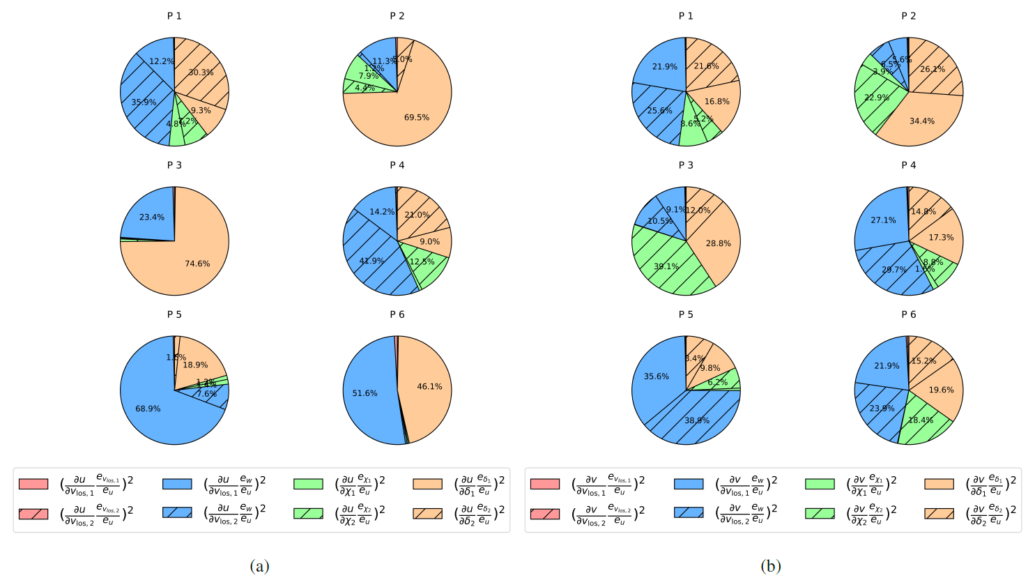
Figure 9Quadratic contributions of the different error terms in the standard uncertainty propagation (SUP) to the (a) longitudinal (eu) and (b) lateral (ev) components at the marker positions P1 to P6.
To visualise the reconstruction accuracy, horizontal velocity profiles are extracted at six upstream streamwise cross sections and compared against the LES in Fig. 10. The shaded region illustrates the total measurement uncertainty where the statistical uncertainty and the propagated uncertainty are summed in quadrature assuming a perfectly calibrated lidar with no measurement bias and uncorrelated errors. This total combined uncertainty accounts for the statistical variability in the measured flow in addition to the variability due to the lidar limitations. The longitudinal velocity profiles measured by the virtual WindScanners at exhibit deviations from the LES due to the large elevation angles required for scanning, while the estimation errors reduce towards WT2. Similarly, very close to the downstream turbine at , the WindScanner-measured u profile is lower compared to the LES close to the rotor axis as the measurement volume extends behind the rotor while scanning very close to the rotor plane. At , the maximum u error is 11.6 %, while the error reduces in the downstream direction with a maximum error of 9.7 % at . The WindScanner-measured u velocity profiles at , and agree well with the LES. Moving further downstream, the difference in the intersection angles of the two lidars decreases. Therefore, the u component is better estimated on the scan's downstream side as the laser beams align with the prevailing wind direction with reducing elevation angles. While the intersection angle reduces towards WT2, the velocity profile at shows slightly larger error bars due to a large vertical wind speed component resulting from local aerodynamic effects close to the rotor plane of WT2. The lateral velocity component profiles show good agreement with the LES, with minor differences seen at the scan edges. The error bars around the v-component profiles are larger than the differences in the LES and WindScanner-resolved profiles due to the inclusion of multiple error terms in the SUP. This indicates that the WindScanners can resolve the two-dimensional velocity profiles with the current setup. While using the local w component in the SUP, it is seen that the observed velocity reconstruction errors are dependent on both the scanning strategy and the flow dynamics.
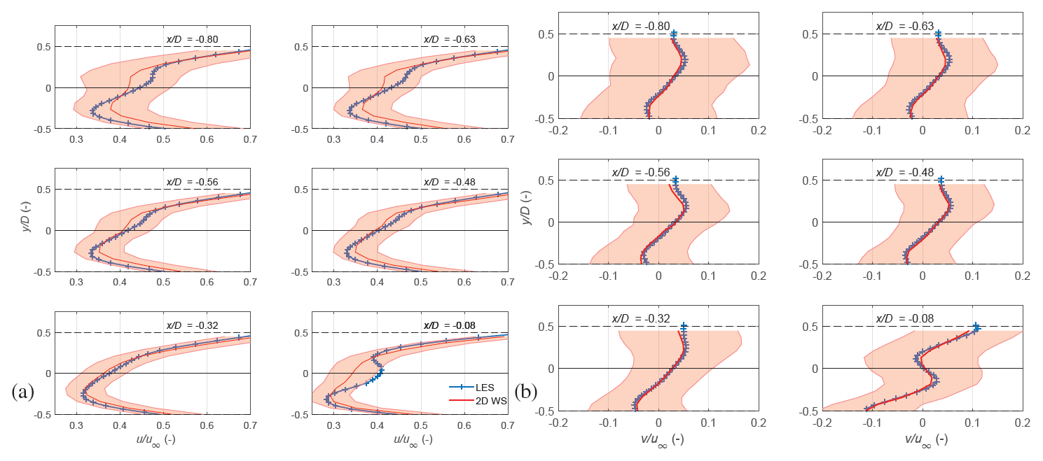
Figure 10WindScanner-estimated velocity profiles (red) of longitudinal (a) and lateral (b) velocities at six upstream cross sections compared against the reference LES (blue). The red-shaded area indicates the total combined measurement uncertainty estimated through Eqs. (7) and (8) using the local w velocity component.
3.2 Measurement results
This section illustrates and discusses the field measurements for the four measurement cases covering scenarios from undisturbed inflow to full- and partial-wake scenarios as described in Table 3. To calculate the propagated uncertainties using field data it is required to assume a constant w. For the full-wake and partial-wake cases, a value of w=1 m s−1 is applied, similar to van Dooren et al. (2017). However, assuming a constant w on the scanning area masks the velocity reconstruction error that is dependent on the flow dynamics, especially close to the rotor. Furthermore, this leads to a larger magnitude of eu and ev compared to the error when using the local w velocities directly.
3.2.1 The undisturbed induction zone
Figure 11 shows the averaged longitudinal and lateral wind velocities extracted from the WindScanner measurements of Case 1 in Table 3 with a mean wind speed of 8.51 m s−1 and a weakly stable stratification. The non-operating upstream turbine had an average yaw misalignment of 3.7°, whereas the downstream turbine had an average misalignment of 0.9° during the measurement period. The extent of the induction zone can be visualised by the u-component deceleration and is very strong within upstream of WT2. This strong velocity deficit can be attributed to high axial induction and weakly stable stratification during the measurement period, inhibiting vertical displacement of air particles and further enhancing the blockage. The induction effect is the strongest at the inboard blade stations and decreases towards the blade tips. The induction zone also exhibits a slightly asymmetrical distribution between the left () and right sides () of the rotor.

Figure 11Case 1: longitudinal (a) and lateral (b) velocities measured while WT1 was not operating and WT2 was operational. In (c), the quiver plot is based on the measured horizontal velocities.
Looking downwind, this slight asymmetry could be attributed to the presence of a tall treeline in between WT1 and WT2 perturbing the flow by acting as a windbreak (Counihan et al., 1974; Tobin et al., 2017) and the strong vertical shear αshear=0.21 that causes a vertical wind speed gradient varying the relative wind speed and the angle of attack of the blades during a rotation. Additionally, the induced velocities at the rotor plane are influenced by the counter-rotating wake, creating a momentum transfer between the lower and upper rotor regions, leading to a difference in flow magnitude between and (Madsen et al., 2012). Hence, the blade sections would experience varying blade forces that vary the local thrust coefficient and the corresponding deceleration. The lateral velocity component is non-zero close to the blade tips, indicating a flow expansion around the rotor. The large lateral velocities present close to the rotor plane can be attributed to the lower data availability due to blade passage; improper tracking of wind direction by WT2, which influences the induced velocities; and neglecting vertical velocity in the dual-Doppler reconstruction. In Fig. 11c, the u and v wind components within the scanning plane are combined to illustrate the wind direction behaviour in the scan plane, exhibiting an induction zone asymmetry and flow expansion around the WT2 rotor.
In Fig. 12, horizontal inflow profiles at five upstream distances moving towards WT2 are plotted. The shaded regions indicate the total measurement uncertainty bounds calculated for the dual-Doppler reconstruction using Eqs. (7) and (8). Here, a constant vertical component w=0.2 m s−1 is assumed, as no wakes propagate from the non-operational upstream turbine, and no direct measurements of the w component were available in the scanned area. The u-component uncertainty due to the dual-Doppler reconstruction decreases moving towards the rotor. The horizontal profiles at exhibit asymmetrical behaviour between the left () and right () blade tips, whereas at , the asymmetry disappears. The magnitude of the velocity deviations lies within the calculated uncertainty bounds. The lateral velocity profiles show a large magnitude very close to the rotor tips due to the flow expansion.

Figure 12Case 1: inflow longitudinal (a) and lateral (b) profiles extracted at various positions upstream of WT2. The shaded area represents the total combined measurement uncertainty calculated from the standard uncertainty propagation method (eu) with w= 0.2 m s−1, as WT1 was not operational.
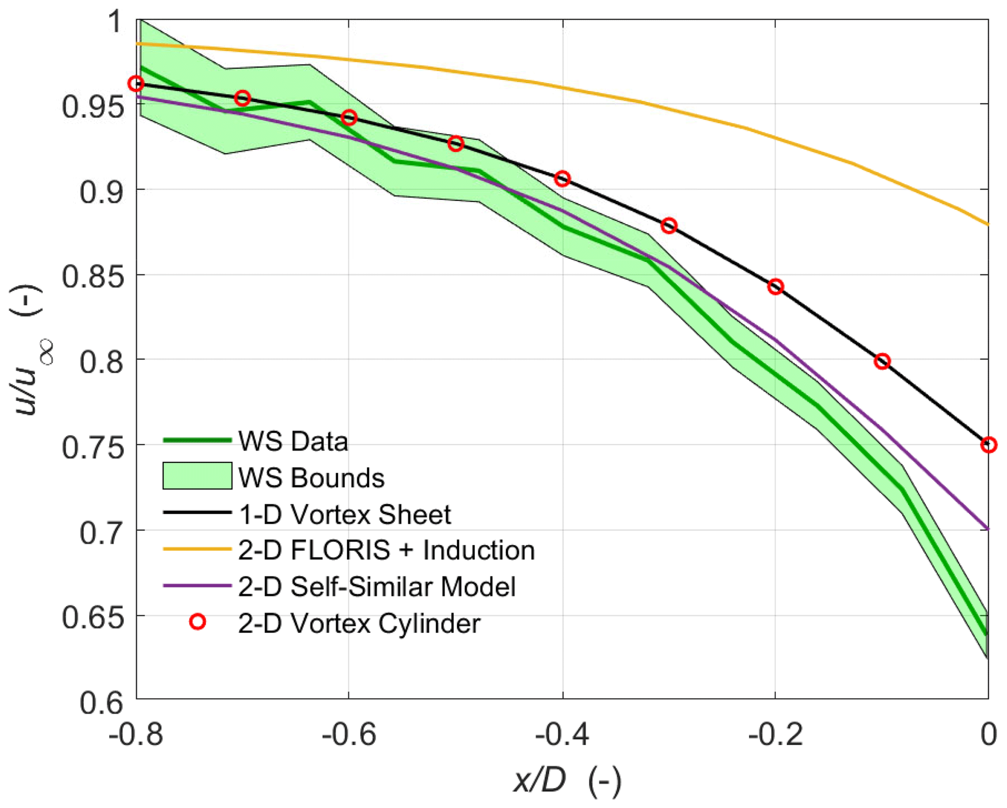
Figure 13Case 1: comparison of the velocity deceleration along the rotor axis against the predictions from different induction zone models. The green-shaded area represents the upper and lower bounds of the total measurement uncertainty.
We compared the different induction zone models against the measurements along the rotor axis, as illustrated in Fig. 13. The upper and lower bounds of the WindScanner represent the propagated uncertainty bounds. Data availability between is reduced due to the presence of the nacelle and therefore excluded. Also plotted is the velocity deceleration predicted by the one-dimensional vortex sheet theory (Medici et al., 2011) using the freestream velocity measured at the met mast, extrapolated to WT2 hub height using the shear exponent, and the axial induction factor of 0.23 estimated from the turbine thrust curve. The model-predicted velocity deceleration falls within the WindScanner bounds until , while the slowdown is under-predicted close to the rotor plane. Simley et al. (2016) also noted similar bias, the reasons for which were that the model does not consider atmospheric stability or the presence of the tower- and nacelle-induced deceleration.
The velocity deceleration predicted by the vortex cylinder (VC) model (Branlard and Gaunaa, 2015), FLORIS coupled with the induction model (FLORIS+Induction) (Branlard and Meyer Forsting, 2020) and the self-similar model (Troldborg and Meyer Forsting, 2017) is also illustrated in Fig. 13 using the inflow conditions in Table 3 as input parameters. Although these models can predict the upstream velocity deceleration in the horizontal plane, they do not consider the vertical shear. Therefore, only the deceleration along the rotor axis is displayed. The FLORIS+Induction model also utilises the said VC method to predict the induction deceleration coupled with the Gaussian wake model in FLORIS accessed from Branlard (2019). As expected, the VC model shows excellent agreement with the one-dimensional vortex sheet results but exhibits an under-prediction of the velocity decrease compared to the measurements. A similar under-prediction of the velocity decrease by the VC model was noted in Meyer Forsting et al. (2021) as no wake expansion is considered to affect the momentum balance upstream and downstream of the rotor, which increases with increasing thrust coefficients. Also shown in Fig. 13 are the results of the self-similar model proposed by Troldborg and Meyer Forsting (2017). Along the rotor axis, the model is similar to the VC model but contains an additional thrust-dependent scaling term to correct for the systematically underestimated axial induction. Applying the thrust correction factor of Troldborg and Meyer Forsting (2017), better agreement with the WindScanner measurements is obtained until . The FLORIS+Induction model consistently under-predicts the magnitude of the velocity decrease along the centre line, with the effect becoming more severe towards the rotor. The axial induction and, therefore, the deceleration obtained from the FLORIS model were lower compared to the field measurements.
3.2.2 The fully waked induction zone
This section presents the results of Case 2, with u∞=9.60 m s−1, and wind veer γ=19.8° in a near-neutral stratification. During the measurement period, the upstream turbine was operated by a greedy controller that introduced an average yaw misalignment of −1.3°, while WT2 was misaligned with an average of 0.6° with the prevailing wind direction. Hence, a full-wake scenario at WT2 occurs. The WindScanners were programmed to perform horizontal scans at the hub height of WT2. This resulted in scans capturing the WT1 wake on a horizontal plane 0.16D above the hub height of WT1 owing to the hub height difference.
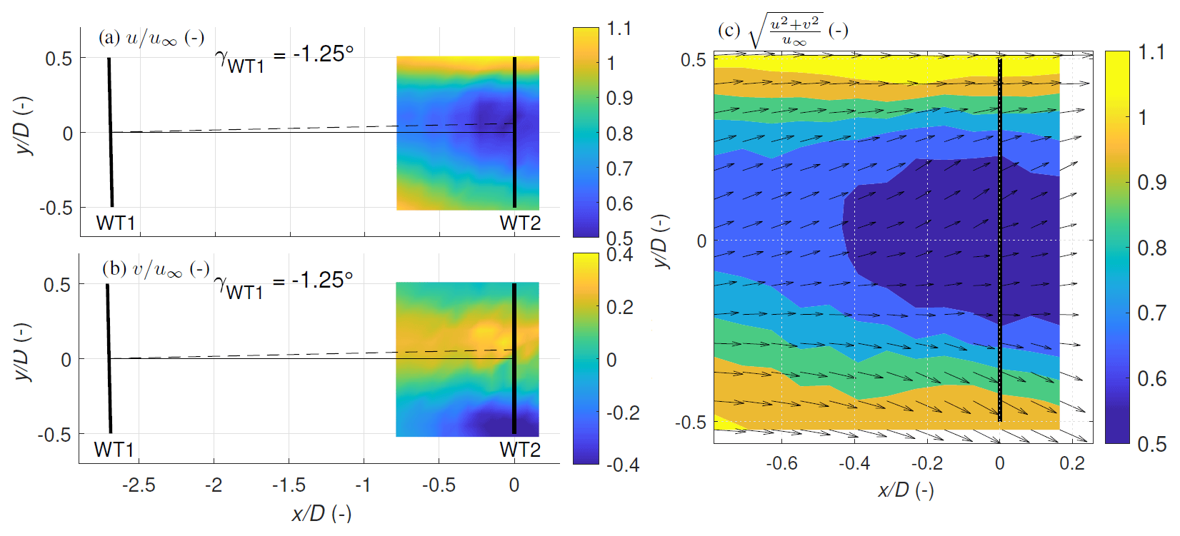
Figure 14Case 2: longitudinal (a) and lateral (b) velocities measured for the full-wake case. The contour of the magnitude of the horizontal velocity and its vector field are plotted in (c).
Due to the downstream turbine operation, an induction zone deceleration is observed inside the wake between upstream of the rotor, as shown in Fig. 14. The lateral velocity component is dominated by a lateral flow towards the left side () of the rotor looking downstream. The flow expansion around the downstream turbine can be observed with stronger lateral velocities on the left side of the rotor () looking downwind. In the region where and , a strong cross-wind component is introduced into the wake that rotates in the opposite direction to that of the clockwise-rotating rotor. By combining the u and v velocities, the local wind vector in the horizontal-scan plane can be estimated. Plotted in Fig. 14c is the total horizontal velocity magnitude U superimposed with streamlines. A clear induction zone is visible centred around the rotor axis in the region where , while the wake is expanded around the strong induction. Due to the proximity between the two turbines, an interaction between the induction zone of the downstream turbine with the wake of the upstream turbine is observed, while the wake deficit is further increased as the induction zone blocks and expands the flow around it.
The horizontal flow profiles were plotted at five locations upstream of WT2, as shown in Fig. 15, to investigate the effect of WT2 induction on the wake profiles. As no measurements of the w component were available, a conservative value of 1 m s−1 has been utilised to estimate the upper and lower uncertainty bounds of the profiles. Instead of recovering, the longitudinal velocity profiles show a deceleration towards WT2. The effect of induction is the strongest close to the rotor axis between , where a velocity reduction of 27 % is observed between and . The lateral velocity component shows a non-zero component between , indicating that the flow is pushed towards the blade tips and around the induction zone. The lateral velocity variations at the blade tips are due to the reduced data availability close to the blades () due to blade passage and the yaw error of the downstream turbine. The turbine does not follow the wind direction perfectly; hence, time-varying yaw errors can be introduced, which would induce movement of the rotor within the scan area, leading to erroneous estimates in the measurements. The lateral velocity profiles at different upstream positions exhibit a slight asymmetry. While terrain heterogeneity could explain some of the measured features, further differences with the undisturbed inflow case are expected due to the WT1 wake and differences in inflow conditions. For Case 2, the inflow is characterised by high shear and veer between the top and bottom rotor blade tips, in contrast to Case 1. This interaction of vertical shear with the wake can lead to an asymmetric velocity distribution as the wake rotation mixes the different layers of fluid in the vertically sheared flow (Sezer-Uzol and Uzol, 2013; Xie and Archer, 2017; Abkar et al., 2018). At all five upstream positions, the wake at exhibited stronger velocity reductions than the wake at ; however, the magnitude of the velocity deviations is within the calculated uncertainty bounds.
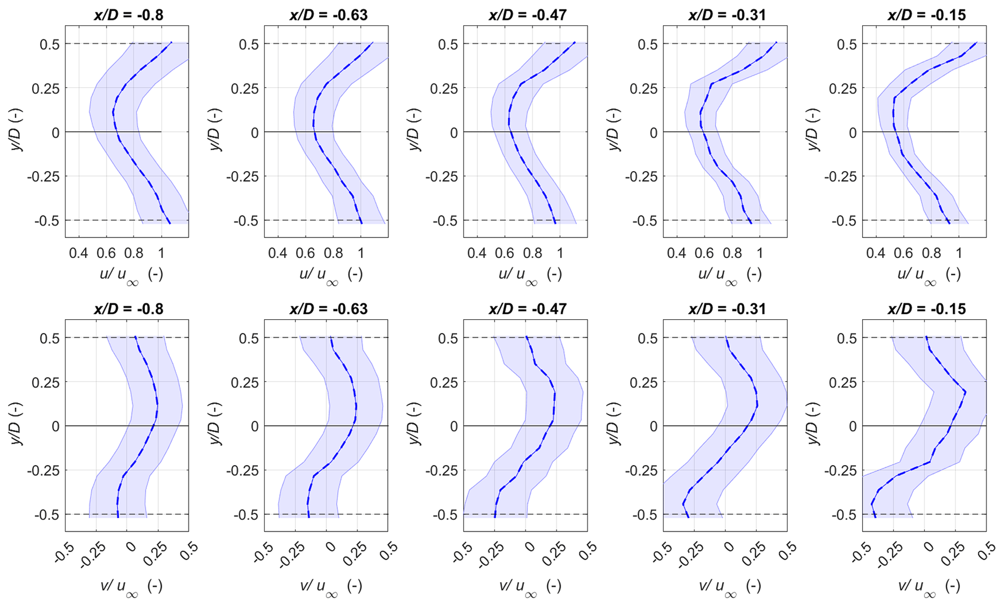
Figure 15Case 2: longitudinal and lateral velocities measured for the full-wake case. The shaded area represents the total combined uncertainty calculated from the standard uncertainty propagation method (eu) with w= 1 m s−1, as WT1 was operational.
3.2.3 The partially waked induction zone
Finally, we present the measurements of the induction zone upstream of WT2 during a partially waked condition shown in Fig. 16. The results for both positive and negative yaw offsets of WT1 are illustrated in Fig. 16. For a positive offset (Case 3: γWT1=12.8°), a wake deflection towards the left of the rotor () is observed in the u component looking downstream, while the wake deflects to the right of the rotor () for the negative offset (Case 4: ). For both cases, the partially waked inflow into WT2 is caused by a combination of the yaw offset applied on WT1 and the misalignment of the wind direction with the orientation of the WT1–WT2 axis. For Case 3, the lateral velocity component is characterised by a flow towards the left side of the rotor () due to a combination of the counter-clockwise wake rotation and the lateral force applied on the flow due to the intentional yawing of the turbine. The opposite effect is observed for Case 4, where a lateral flow towards the right side of the rotor plane is seen. The findings correspond to Fleming et al. (2018), where a stronger wake deflection for the positive yaw case is seen due to the aggregated effect of the wake rotation and counter-rotating vortices in comparison to the negative deflection case.

Figure 16Cases 3 and 4: longitudinal and lateral velocities measured for positive yaw offset (Case 3, a, b) and negative yaw offset (Case 4, c, d). The dashed red line represents the average wind direction during the measurement period.
In both cases, the maximum magnitude of the lateral velocity inside the deflected wake is approximately 0.2 u∞ to 0.25 u∞. The positive yaw offset case exhibits a comparatively more substantial lateral flow component compared to the negative yaw offset due to the 10° misalignment between the turbine orientation and the wind direction as the lateral velocity would be increased by the projection of misaligned inflow into the defined coordinate system. As the measurements are in the near-wake region of WT1, the lateral velocity would be additionally influenced by the aerodynamic effects of the rotor, while the effect of yaw steering on the lateral component would be dominant further downstream. In both cases, the lateral component increases towards the blade tips to account for the flow expansion close to the downstream turbine. It is noted that for the positive offset case, the spatial distribution of the u component seems to move near the rotor axis instead of deflecting towards . This could be potentially attributed to the 10° misalignment between the wind direction and the turbine orientation direction in addition to the large variability of the wind direction from 208 to 223°, which was the highest of all investigated cases.
Figure 17 illustrates the horizontal wake profiles of the longitudinal and lateral velocities at five distances upstream of WT2 for the two wake deflection cases. The dots correspond to the wake centre position determined by fitting a Gaussian through the measured wake profiles (Hulsman et al., 2022b). For the positive offset γWT1=12.8°, the wake centre deflects further to the left of the rotor to approximately . Similarly, the wake centre is deflected to the right to approximately for negative offset . In both cases, the wake centre in the horizontal profiles does not exhibit significant lateral movement, evidenced by the clustered wake centre locations in Fig. 17. In both cases, a yaw-induced lateral flow is observed inside the deflected wake with a magnitude depending on the yaw offset and is present at the location of the maximum velocity deficit.

Figure 17Cases 3 and 4: wake profiles of the normalised longitudinal component (a, b) and the lateral velocity (c, d) extracted at various positions upstream of WT2 during active wake steering at WT1. The dots correspond to the wake centre at each location. The shaded area represents the total combined uncertainty calculated using the SUP method with w=1 m s−1.
We characterise the interaction of the near wake and the induction zone between two closely spaced turbines with two synchronised scanning lidars. During the measurement campaign, yaw control is implemented on the upstream turbine. Hence, two-dimensional characterisation of the induction zone of the downstream turbine is achieved for unwaked, waked and partially waked conditions.
Measurement campaigns require a comprehensive description of the measurement setup and appropriate uncertainty quantification to interpret results. As only two lidars were available for the experiment, an assumption on the vertical flow component, e.g. w=0 m s−1, for the dual-Doppler reconstruction is necessary to extract two-dimensional horizontal flow fields. The location of the lidar and scanning trajectory have a significant impact on the measured velocity profiles. Therefore, to quantify the effect of the measurement setup and WindScanner limitations, we simulate the measurement scenario using a high-fidelity LES and a lidar simulator. Although such simulations might not completely capture the spatio-temporal dynamics observed in the field, they provide a complementary methodology for performance and quality assessment.
A comparison between the LES and the virtually simulated WindScanner indicates that the WindScanners can capture the main flow structures within a horizontal plane despite the assumption used (w=0 m s−1) and the inherent measurement principle limitations, such as directional bias and probe volume averaging. Analysis of the statistical and propagated uncertainties revealed that the former had in comparison a smaller uncertainty. For the longitudinal component, a maximum statistical uncertainty of 5 % and a maximum propagated uncertainty of 15 % relative to the mean wind speed were observed. A deeper analysis of the propagated uncertainties indicated that the main contribution to the uncertainty to estimate the u and v components was the w=0 m s−1 assumption. Other important sources of the uncertainty were the probe volume-averaging effect, the inaccuracy of the beam intersection angles and the beam pointing errors.
The simulations highlight that spatial error variation also depends on the local vertical velocity distribution in the scanning area. This means that the reconstruction accuracy is not only lidar dependent but also flow field dependent. Furthermore, the combination of the lidar-dependent errors and the vertical velocity increases the error, especially for a large elevation angle δ. Because no local vertical velocity measurements were available in the scanning area, a local vertical assumption was required to conduct the SUP. Therefore, the approach of van Dooren et al. (2016) was followed by assuming a conservative vertical velocity of either 0.2 m s−1 (unwaked) or 1 m s−1 (waked) over the scanning area. This assumption masks the influence of the flow dynamics on the propagated errors and significantly increases the magnitude of the propagated errors. This complicates the analyses with respect to determining significant flow features from field measurements, especially in waked cases. Further measurements with a third synchronised lidar are suggested to avoid the assumption of neglecting the vertical velocity and provide measurements with a lower uncertainty in the flow within the induction zone.
In the second part of this study, the full-scale experimental measurements using synchronised scanning lidar systems are analysed. Although accurate spatial and temporal synchronisation was achieved after careful calibration in the field, uncertainties inherent in the scanning lidar measurements need to be evaluated. The applied error of 0.1 % for vlos might be low for this measurement campaign. The work of Pedersen and Courtney (2021) suggested a 0.1 % error in a highly controlled environment. van Dooren et al. (2022) used the same WindScanner lidars in a wind tunnel study and quantified the error against a hot-wire anemometer with a mean average error metric of less than 2 %. However, the probe lengths in their study were of the order of 13 cm. In the current field measurements, probe lengths of the order of 6.75 to 27.75 m are measured, increasing the expected error. Further measurements are required to obtain a representative evlos. This can be achieved by focusing the lidar next to a sonic anemometer to determine the impact of the probe volume effect on the line-of-sight measurements. Further WindScanner simulations indicated that the total propagated error was insensitive to a higher and more realistic 2 % line-of-sight error. An important aspect to consider during cw scanning measurements is the trade-off between spatial and temporal resolution. With a slower scan speed, the measurements cannot capture the fluctuating behaviour of the flow but only a fingerprint of the highly turbulent near wake. Moreover, the variable probe length during the scan causes a focal-distance-dependent bias and therefore a variable low-pass-filtering effect throughout the scan. Correcting for this effect is a challenging task and requires precise knowledge of the filtered and unfiltered spectra to either construct or model a transfer function (Angelou et al., 2012; van Dooren et al., 2022). This was not performed in the current measurements.
As expected, the measurements reveal the influences of the wake of WT1 on the induction zone of WT2. A longitudinal speed reduction towards the rotor plane is observed in the free inflow case. The lateral component shows a non-zero speed component towards the edges of the rotor, which indicates a flow expansion. An asymmetrical induction zone at hub height was also recorded and can be caused by multiple effects. This asymmetry can potentially be attributed to the dynamic interaction between the vertical shear and the rotating blades, which was noted by Bastankhah and Porte-Agel (2017) using wind tunnel measurements. Madsen et al. (2012) suggested that the induction zone at the rotor plane could be influenced by the counter-rotating wake creating a momentum transfer between the different rotor areas. Another possible effect of the observed asymmetry is the presence of a long and staggered treeline between the two turbines, which acts as a windbreak to the flow, perturbing in the region between the two turbines (Counihan et al., 1974; Tobin et al., 2017). Previous studies at the site (Hulsman et al., 2022a) have indicated the influence of a treeline on the met mast measurements at 100 m elevation by comparing the measurements against the ground-based lidar. A possible flow diversion by the treeline would indicate a larger vertical velocity component. This will lead to a larger uncertainty due to the necessary assumption of w=0 m s−1 to apply the dual-Doppler reconstruction. The magnitude of these terrain effects on the flow and the lidar measurements could not be quantified as no measurements were available when both turbines were non-operational. A high-resolution LES study incorporating the terrain and the treeline could be used to provide insights into the flow behaviour. However, the LES runs were intended to study the lidar measurement accuracy and were therefore only initialised with a roughness length similar to the terrain.
An evaluation of various induction zone models is conducted, highlighting that the velocity deceleration modelled by the self-similar model (Troldborg and Meyer Forsting, 2017) is in good agreement with the measurement data. More measurements covering more extensive operating and stability regimes would provide more insight. When both turbines were operational and aligned with the prevailing θwdir (fully waked), a clear overlap of the wake of WT1 and the induction zone of WT2 was observed. While vertical-plane scans would have revealed the vertical shear and veer interaction with the wake, this was not investigated in the current study. The measurements during yaw steering show partial-wake conditions impinging on either side of the rotor. It was expected that due to the partial-wake inflow into WT2, the aerodynamic induction between the waked and unwaked parts of the rotor would differ, impacting the distribution of induction zone deceleration over the rotor. However, these effects were not quantified in our study as the measured effects were within the uncertainty bounds of the measurements and therefore not significant enough. Additional measurements during partial-wake conditions would be beneficial, especially with a third synchronised lidar, to study these interactions. While the hub height difference of 20 m between the two turbines would influence the measured induction zone and wake interaction, the effect could not be characterised as the presented study is specific to this two-turbine layout. The results of this study are based on four measurement cases containing two-dimensional flow within a horizontal scan performed at the hub height of the downstream turbine. However, future investigations should include measurements conducted with turbines at the same hub height and measure vertical planes or full rotor planes. This will aid in investigating the influence of atmospheric effects such as wind shear and veer. Multiple vertical-plane measurements can also be performed to study the evolution of the flow field between the two turbines. A longer measurement campaign covering a range of shear and veer conditions, including negligible veer and shear, is suggested to investigate any possible correlations between atmospheric effects and the behaviour of the induction zone.
In this paper, results of a measurement campaign using two synchronised WindScanner lidars, which were used to capture the flow between two 3.5 MW utility-size turbines spaced 2.7 diameters (D=126 m) apart, are presented. The lidar measurements were further supported by a ground-based lidar, a met mast and an eddy covariance station to accurately characterise the inflow. A detailed error analysis is performed by recreating the measurement procedure in a large-eddy simulation where two virtual WindScanners were simulated to evaluate the dual-Doppler reconstruction accuracy. The reconstruction accuracy is influenced by the limitations of the measurement device, the reconstruction principle and the spatial variability of the vertical flow. The narrow turbine spacing and active wake steering on the upstream turbine allowed for the characterisation of the induction zone flow behaviour for free inflow, fully waked and partially waked scenarios. To the best of the authors' knowledge, capturing the two-dimensional flow within both the near wake and the induction zone during an intentional yaw misalignment in the field is measured for the first time. For a fully waked inflow, the impact of the induction zone on the wake was observed. This increased the wake deficit close to the rotor.
The study further highlights the challenges in conducting field measurements and the additional considerations needed to characterise the induction zone behaviour. As field data are accepted as the ground truth and demanded for validating numerical models, a thorough characterisation of the site, the lidars, the measurements and their associated uncertainties is provided to ensure comprehensive traceability of the measurements. Further measurements, covering a larger range of inflow scenarios, preferably with a third synchronised lidar to avoid neglecting the vertical velocity in the dual-Doppler reconstruction, in conjunction with high-resolution simulations, are suggested for further work to obtain a deeper understanding of the induction zone behaviour for various operational states of the turbine.
The turbine operational data cannot be made public due to an existing non-disclosure agreement with the operator. The lidar and inflow data can be made available on request.
APKS and PH prepared and installed the WindScanner setup of the experiment and jointly measured the data. APKS focused on the measurements in a horizontal plane of the induction zone, while PH mainly dealt with investigating the vertical plane (not shown in this paper). APKS and PH analysed the measurement data obtained by the WindScanner, the met mast and the two turbines. APKS performed the virtual WindScanner simulations, extended the uncertainty quantification methodology and wrote the paper, while PH calibrated the turbine model and executed the LES runs. APKS interpreted the WindScanner results with regard to the induction zone. PH analysed and prepared the VAD data for further use. MFvD assisted during the design and execution of the measurement campaign, helped interpret the data, and contributed to the uncertainty quantification methodology. MK was involved in the design of the measurement campaign, provided extensive reviews and had a supervisory role. All authors contributed to fruitful discussions and reviewed the paper.
The contact author has declared that none of the authors has any competing interests.
Publisher’s note: Copernicus Publications remains neutral with regard to jurisdictional claims made in the text, published maps, institutional affiliations, or any other geographical representation in this paper. While Copernicus Publications makes every effort to include appropriate place names, the final responsibility lies with the authors.
This work was partly funded by the Federal Ministry for Economic Affairs and Energy according to a resolution by the German Federal Parliament, in the scope of the research projects DFWind (ref. no. 0325936C) and CompactWind II (ref. no. 0325492H). We acknowledge Eno Energy Systems GmbH for their support during the measurements. Special mention is given to Stephan Stone for his major support during the measurement campaign and to Andreas Rott for discussions regarding the uncertainty quantification. We also acknowledge Torben Mikkelsen, Mikael Sjoholm and Claus Brian Munk Pedersen from the Technical University of Denmark for sharing their expertise on the WindScanner systems and for their support in solving technical issues.
This research has been supported by the Bundesministerium für Wirtschaft und Energie (DFWind (ref. no. 0325936C) and CompactWind II (ref. no. 0325492H)).
This paper was edited by Rebecca Barthelmie and reviewed by three anonymous referees.
Abkar, M., Sørensen, J. N., and Porté-Agel, F.: An Analytical Model for the Effect of Vertical Wind Veer on Wind Turbine Wakes, Energies, 11, 1838, https://doi.org/10.3390/EN11071838, 2018. a
Angelou, N., Mann, J., Sjöholm, M., and Courtney, M.: Direct measurement of the spectral transfer function of a laser based anemometer, Rev. Sci. Instrum., 83, 033111, https://doi.org/10.1063/1.3697728, 2012. a, b
Angelou, N., Mann, J., and Dellwik, E.: Scanning Doppler lidar measurements of drag force on a solitary tree, J. Fluid Mech., 917, A30, https://doi.org/10.1017/jfm.2021.275, 2021. a
Asimakopoulos, M., Clive, P., More, G., and Boddington, R.: Offshore compression zone measurement and visualization, in: European Wind Energy Association 2014 Annual Event, Barcelona, Spain, 2014. a
Barthelmie, R. J.: The effects of atmospheric stability on coastal wind climates, Meteorol. Appl., 6, 39–47, https://doi.org/10.1017/S1350482799000961, 1999. a
Bastankhah, M. and Porte-Agel, F.: Wind tunnel study of the wind turbine interaction with a boundary-layer flow: Upwind region, turbine performance, and wake region, Phys. Fluids, 29, 065105, https://doi.org/10.1063/1.4984078, 2017. a
Beck, H. and Kühn, M.: Dynamic Data Filtering of Long-Range Doppler LiDAR Wind Speed Measurements, Remote Sensing, 9, 561, https://doi.org/10.3390/rs9060561, 2017. a
Branlard, E.: Wiz, wake and induction zone model, GitHub [code], https://github.com/ebranlard/wiz (last access: 23 April 2022), 2019. a
Branlard, E. and Gaunaa, M.: Cylindrical vortex wake model: right cylinder, Wind Energy, 18, 1973–1987, https://doi.org/10.1002/WE.1800, 2015. a, b, c
Branlard, E. and Meyer Forsting, A. R.: Assessing the blockage effect of wind turbines and wind farms using an analytical vortex model, Wind Energy, 23, 2068–2086, https://doi.org/10.1002/we.2546, 2020. a, b
Bromm, M., Rott, A., Beck, H., Vollmer, L., Steinfeld, G., and Kühn, M.: Field investigation on the influence of yaw misalignment on the propagation of wind turbine wakes, Wind Energy, 21, 1011–1028, https://doi.org/10.1002/we.2210, 2018. a, b
Cheynet, E., Jakobsen, J. B., Snæbjörnsson, J., Mikkelsen, T., Sjöholm, M., Mann, J., Hansen, P., Angelou, N., and Svardal, B.: Application of short-range dual-Doppler lidars to evaluate the coherence of turbulence, Exp. Fluids, 57, 184, https://doi.org/10.1007/s00348-016-2275-9, 2016. a
Counihan, J., Hunt, J. C., and Jackson, P. S.: Wakes behind two-dimensional surface obstacles in turbulent boundary layers, J. Fluid Mech., 64, 529–564, https://doi.org/10.1017/S0022112074002539, 1974. a, b, c
Debnath, M., Doubrawa, P., Herges, T., Martínez-Tossas, L. A., Maniaci, D. C., and Moriarty, P.: Evaluation of Wind Speed Retrieval from Continuous-Wave Lidar Measurements of a Wind Turbine Wake Using Virtual Lidar Techniques, J. Phys. Conf. Ser., 1256, 012008, https://doi.org/10.1088/1742-6596/1256/1/012008, 2019. a
Dunne, F., Pao, L. Y., Schlipf, D., and Scholbrock, A. K.: Importance of lidar measurement timing accuracy for wind turbine control, P. Amer. Contr. Conf., 3716–3721, https://doi.org/10.1109/ACC.2014.6859337, 2014. a
Fleming, P., Annoni, J., Churchfield, M., Martinez-Tossas, L. A., Gruchalla, K., Lawson, M., and Moriarty, P.: A simulation study demonstrating the importance of large-scale trailing vortices in wake steering, Wind Energ. Sci., 3, 243–255, https://doi.org/10.5194/wes-3-243-2018, 2018. a
Giyanani, A., Sjöholm, M., Rolighed Thorsen, G., Schuhmacher, J., and Gottschall, J.: Wind speed reconstruction from three synchronized short-range WindScanner lidars in a large wind turbine inflow field campaign and the associated uncertainties, J. Phys. Conf. Ser., 2265, 022032, https://doi.org/10.1088/1742-6596/2265/2/022032, 2022. a, b, c
Göçmen, T., Laan, P. V. D., Réthoré, P. E., Diaz, A. P., Larsen, G. C., and Ott, S.: Wind turbine wake models developed at the technical university of Denmark: A review, Renew. Sust. Energ. Rev., 60, 752–769, https://doi.org/10.1016/J.RSER.2016.01.113, 2016. a
Hulsman, P., Sucameli, C., Petrović, V., Rott, A., Gerds, A., and Kühn, M.: Turbine power loss during yaw-misaligned free field tests at different atmospheric conditions, J. Phys. Conf. Ser., 2265, 032074, https://doi.org/10.1088/1742-6596/2265/3/032074, 2022a. a, b, c
Hulsman, P., Wosnik, M., Petrović, V., Hölling, M., and Kühn, M.: Development of a curled wake of a yawed wind turbine under turbulent and sheared inflow, Wind Energ. Sci., 7, 237–257, https://doi.org/10.5194/wes-7-237-2022, 2022b. a, b
International Electrotechnical Commission: Wind turbines, Part 12-1: Power performance measurements of electricity producing wind turbines,, International Electrotechnical Commission, 3 Edn. , 2005, 179, https://webstore.iec.ch/publication/68499 (last access: 8 July 2024), 2022. a
Jiménez, Ã., Crespo, A., and Migoya, E.: Application of a LES technique to characterize the wake deflection of a wind turbine in yaw, Wind Energy, 13, 559–572, https://doi.org/10.1002/we.380, 2009. a
Jonkman, J. M. and Buhl Jr., M. L.: FAST user's guide, National Renewable Energy Laboratory, Golden, CO, Technical Report No. NREL/EL-500-38230, https://www.nrel.gov/docs/fy06osti/38230.pdf (last access: 5 July 2024), 2005. a
Kelley, C. L., Herges, T. G., Martinez, L. A., and Mikkelsen, T.: Wind turbine aerodynamic measurements using a scanning lidar, J. Phys. Conf. Ser., 1037, 052014, https://doi.org/10.1088/1742-6596/1037/5/052014, 2018. a
Krüger, S., Steinfeld, G., Kraft, M., and Lukassen, L. J.: Validation of a coupled atmospheric–aeroelastic model system for wind turbine power and load calculations, Wind Energ. Sci., 7, 323–344, https://doi.org/10.5194/wes-7-323-2022, 2022. a
Lund, T. S., Wu, X., and Squires, K. D.: Generation of Turbulent Inflow Data for Spatially-Developing Boundary Layer Simulations, J. Comput. Phys., 140, 233–258, https://doi.org/10.1006/jcph.1998.5882, 1998. a
Lundquist, J. K., Churchfield, M. J., Lee, S., and Clifton, A.: Quantifying error of lidar and sodar Doppler beam swinging measurements of wind turbine wakes using computational fluid dynamics, Atmos. Meas. Tech., 8, 907–920, https://doi.org/10.5194/amt-8-907-2015, 2015. a
Madsen, H. A., Riziotis, V., Zahle, F., Hansen, M. O., Snel, H., Grasso, F., Larsen, T. J., Politis, E., and Rasmussen, F.: Blade element momentum modeling of inflow with shear in comparison with advanced model results, Wind Energy, 15, 63–81, https://doi.org/10.1002/we.493, 2012. a, b
Maronga, B., Gryschka, M., Heinze, R., Hoffmann, F., Kanani-Sühring, F., Keck, M., Ketelsen, K., Letzel, M. O., Sühring, M., and Raasch, S.: The Parallelized Large-Eddy Simulation Model (PALM) version 4.0 for atmospheric and oceanic flows: model formulation, recent developments, and future perspectives, Geosci. Model Dev., 8, 2515–2551, https://doi.org/10.5194/gmd-8-2515-2015, 2015. a
Medici, D., Ivanell, S., Dahlberg, J.-Ã., and Alfredsson, P. H.: The upstream flow of a wind turbine: blockage effect, Wind Energy, 14, 691–697, https://doi.org/10.1002/we.451, 2011. a, b, c
Meyer Forsting, A., Rathmann, O., Laan, M. v. d., Troldborg, N., Gribben, B., Hawkes, G., and Branlard, E.: Verification of induction zone models for wind farm annual energy production estimation (2019 J. Phys.: Conf. Ser. 1934 012023), J. Phys. Conf. Ser., 1934, 012024, https://doi.org/10.1088/1742-6596/1934/1/012024, 2021. a
Meyer Forsting, A. R., Troldborg, N., and Borraccino, A.: Modelling lidar volume-averaging and its significance to wind turbine wake measurements, J. Phys. Conf. Ser., 854, 012014, https://doi.org/10.1088/1742-6596/854/1/012014, 2017. a
Mikkelsen, T., Sjöholm, M., Angelou, N., and Mann, J.: 3D WindScanner lidar measurements of wind and turbulence around wind turbines, buildings and bridges, IOP Conf. Ser.-Mat. Sci., 276, 012004, https://doi.org/10.1088/1757-899X/276/1/012004, 2017. a
Mikkelsen, T., Sjöholm, M., Astrup, P., Peña, A., Larsen, G., van Dooren, M. F., and Kidambi Sekar, A. P.: Lidar Scanning of Induction Zone Wind Fields over Sloping Terrain, J. Phys. Conf. Ser., 1452, 012081, https://doi.org/10.1088/1742-6596/1452/1/012081, 2020. a
Monin, A. S. and Obukhov, A. M.: Basic laws of turbulent mixing in the surface layer of the atmosphere, Tr. Akad. Nauk SSSR Geophiz. Inst, 24, 163–187, https://gibbs.science/efd/handouts/monin_obukhov_1954.pdf (last access: 7 July 2024), 1954. a
NREL: FLORIS. Version 3.4, GitHub [code], https://github.com/NREL/floris, 2023. a
Pedersen, A. T. and Courtney, M.: Flywheel calibration of a continuous-wave coherent Doppler wind lidar, Atmos. Meas. Tech., 14, 889–903, https://doi.org/10.5194/amt-14-889-2021, 2021. a, b
Peña, A. and Mann, J.: Turbulence Measurements with Dual-Doppler Scanning Lidars, Remote Sensing, 11, 2444, https://doi.org/10.3390/rs11202444, 2019. a
Rahlves, C., Beyrich, F., and Raasch, S.: Scan strategies for wind profiling with Doppler lidar – an large-eddy simulation (LES)-based evaluation, Atmos. Meas. Tech., 15, 2839–2856, https://doi.org/10.5194/amt-15-2839-2022, 2022. a
Robey, R. and Lundquist, J. K.: Behavior and mechanisms of Doppler wind lidar error in varying stability regimes, Atmos. Meas. Tech., 15, 4585–4622, https://doi.org/10.5194/amt-15-4585-2022, 2022. a
Schneemann, J., Theuer, F., Rott, A., Dörenkämper, M., and Kühn, M.: Offshore wind farm global blockage measured with scanning lidar, Wind Energ. Sci., 6, 521–538, https://doi.org/10.5194/wes-6-521-2021, 2021. a
Sengers, B. A. M., Steinfeld, G., Hulsman, P., and Kühn, M.: Validation of an interpretable data-driven wake model using lidar measurements from a field wake steering experiment, Wind Energ. Sci., 8, 747–770, https://doi.org/10.5194/wes-8-747-2023, 2023. a
Sezer-Uzol, N. and Uzol, O.: Effect of steady and transient wind shear on the wake structure and performance of a horizontal axis wind turbine rotor, Wind Energy, 16, 1–17, https://doi.org/10.1002/WE.514, 2013. a
Simley, E., Angelou, N., Mikkelsen, T., Sjöholm, M., Mann, J., and Pao, L. Y.: Characterization of wind velocities in the upstream induction zone of a wind turbine using scanning continuous-wave lidars, J. Renew. Sustain. Ener., 8, 013301, https://doi.org/10.1063/1.4940025, 2016. a, b, c, d, e, f, g
Sjöholm, M., Angelou, N., Hansen, P., Hansen, K. H., Mikkelsen, T., Haga, S., Silgjerd, J. A., and Starsmore, N.: Two-Dimensional Rotorcraft Downwash Flow Field Measurements by Lidar-Based Wind Scanners with Agile Beam Steering, J. Atmos. Ocean. Tech., 31, 930–937, https://doi.org/10.1175/JTECH-D-13-00010.1, 2014. a
Slinger, C. W., Harris, M., and Pitter, M.: Wind speed measurement for absolute power curve determination from induction zone lidar measurements, J. Phys. Conf. Ser., 1618, 032027, https://doi.org/10.1088/1742-6596/1618/3/032027, 2020. a
Sonnenschein, C. M. and Horrigan, F. A.: Signal-to-Noise Relationships for Coaxial Systems that Heterodyne Backscatter from the Atmosphere, Appl. Opt., 10, 1600, https://doi.org/10.1364/ao.10.001600, 1971. a
Stawiarski, C., Traumner, K., Knigge, C., and Calhoun, R.: Scopes and challenges of dual-doppler lidar wind measurements-an error analysis, J. Atmos. Ocean. Tech., 30, 2044–2062, https://doi.org/10.1175/JTECH-D-12-00244.1, 2013. a, b
Tennekes and Lumley: A First Course in Turbulence, The MIT Press, ISBN 9780262536301, https://mitpress.mit.edu/9780262536301/a-first-course-in-turbulence/ (last access: 5 July 2024), 2018. a
Tobin, N., Hamed, A. M., and Chamorro, L. P.: Fractional Flow Speed-Up from Porous Windbreaks for Enhanced Wind-Turbine Power, Bound.-Lay. Meteorol., 163, 253–271, https://doi.org/10.1007/s10546-016-0228-8, 2017. a, b
Trabucchi, D.: Lidar Measurements and Engineering Modelling of Wind Turbine Wakes, PhD thesis, Carl von Ossietzky Universitat Oldenburg, https://www.shaker.de/de/content/catalogue/index.asp?lang=de&ID=8&ISBN=978-3-8440-7516-8 (last access: 5 July 2024), 2020. a
Troldborg, N. and Meyer Forsting, A. R.: A simple model of the wind turbine induction zone derived from numerical simulations, Wind Energy, 20, 2011–2020, https://doi.org/10.1002/we.2137, 2017. a, b, c, d, e, f
Trujillo, J. J., Bingöl, F., Larsen, G. C., Mann, J., and Kühn, M.: Light detection and ranging measurements of wake dynamics. Part II: Two-dimensional scanning, Wind Energy, 14, 61–75, https://doi.org/10.1002/we.402, 2011. a
van Dooren, M. F., Trabucchi, D., and Kühn, M.: A methodology for the reconstruction of 2D horizontal wind fields of wind turbinewakes based on dual-Doppler lidar measurements, Remote Sensing, 8, 809, https://doi.org/10.3390/rs8100809, 2016. a
van Dooren, M. F., Campagnolo, F., Sjöholm, M., Angelou, N., Mikkelsen, T., and Kühn, M.: Demonstration and uncertainty analysis of synchronised scanning lidar measurements of 2-D velocity fields in a boundary-layer wind tunnel, Wind Energ. Sci., 2, 329–341, https://doi.org/10.5194/wes-2-329-2017, 2017. a, b, c, d, e
van Dooren, M. F., Kidambi Sekar, A. P., Neuhaus, L., Mikkelsen, T., Hölling, M., and Kühn, M.: Modelling the spectral shape of continuous-wave lidar measurements in a turbulent wind tunnel, Atmos. Meas. Tech., 15, 1355–1372, https://doi.org/10.5194/amt-15-1355-2022, 2022. a, b, c, d, e
Werner, C. and Streicher, J.: Lidar: Range-Resolved Optical Remote Sensing of the Atmosphere, Springer, 102, ISBN 0-387-40075-3, 2005. a
Wilks, D. S.: Statistical Methods in the Atmospheric Sciences, Fourth Edition, Statistical Methods in the Atmospheric Sciences, Fourth Edition, Elsevier, 1–818, https://doi.org/10.1016/C2017-0-03921-6, 2019. a
Wyngaard, J. C.: Turbulence in the Atmosphere, Cambridge University Press, Cambridge, ISBN 9780521887694, https://doi.org/10.1017/CBO9780511840524, 2010. a
Xie, S. and Archer, C. L.: A Numerical Study of Wind-Turbine Wakes for Three Atmospheric Stability Conditions, Bound.-Lay. Meteorol., 165, 87–112, https://doi.org/10.1007/s10546-017-0259-9, 2017. a