On the importance of wind predictions in wake steering optimization

Wake steering is a technique that optimizes the energy production of a wind farm by employing yaw control to misalign upstream turbines with the incoming wind direction. This work highlights the important dependence between wind direction variations and wake steering optimization. The problem is formalized over time as the succession of multiple steady-state yaw control problems interconnected by the rotational constraints of the turbines and the evolution of the wind. Then, this work proposes a reformulation of the yaw optimization problem of each time step by augmenting the objective function by a new heuristic based on a wind prediction. The heuristic acts as a penalization for the optimization, encouraging solutions that will guarantee future energy production. Finally, a synthetic sensitivity analysis of the wind direction variations and wake steering optimization is conducted. Because of the rotational constraints of the turbines, as the magnitude of the wind direction fluctuations increases, the importance of considering wind prediction in a steady-state optimization is empirically demonstrated. The heuristic proposed in this work greatly improves the performance of controllers and significantly reduces the complexity of the original sequential decision problem by decreasing the number of decision variables.

1 Introduction

As global energy consumption increases, there is a strong willingness and necessity to decarbonize electricity production. Hence, renewable energies are becoming increasingly important (Chu and Majumdar, 2012). Wind energy, particularly, is the focus of considerable research and development, with turbines becoming larger and more numerous within wind farms. Ensuring efficient control as wind turbines operate is necessary to maximize the benefits of wind energy.

In the context of global warming, designing more efficient wind farms is essential. Wake steering is the subject of growing interest within the community to optimize the energy production of wind farms. However, most research regarding wind farm control technologies disregards the relevance of the wind direction variation. This work is motivated by a central question: from what magnitude of wind direction fluctuations is it necessary to consider the wind evolution in a wake steering optimization? To answer this question, this work proposes a new controller based on wind predictions and conducts a synthetic sensitivity analysis of wake steering and wind evolution using steady-state models and artificial wind data.

In wind farm optimization, the use of low-fidelity models (usually based on steady-state models) is favored over higher-fidelity models (usually based on computational fluid dynamics and real-time wake interaction) due to the complexity and computational load associated with solving dynamic equations for every turbine in the farm. Some recent works such as Janssens and Meyers (2024) explore real-time optimal control of wind farms using large-eddy simulations (LESs). However, this research area is still in the early stages and for large-scale wind farm optimization, steady-state models are still widely used.

In wind farm flow control (WFFC), developing effective closed-loop controllers is essential for scaling to larger wind farms and dealing with unpredictable wind conditions. These controllers dynamically adapt their strategies in real time using continuous sensor feedback to guide their decisions. Model-based, closed-loop controllers, in particular, rely on simulators of the environment to conduct continuous optimization while the farm is in operation. Fast and computationally efficient simulation is crucial for these controllers to quickly react to wind and turbines changes. This work focuses on the optimization process itself, adhering to community standards by using widely accepted, open-source, low-fidelity simulators.

1.1 Wake effect

A single wind turbine reaches its maximum power output when fully aligned with the wind. When the wind direction changes, a turbine uses its yaw to rotate its nacelle on a horizontal plane. By using active yaw control, a wind turbine can keep track of the changes in the wind direction and ensure maximum energy production over time by minimizing its misalignment with the wind. It corresponds to greedy control, where a wind turbine solely tries to maximize its power output (Yang et al., 2021).

In the space immediately behind a turbine, the wind speed is slower and more turbulent. Such a phenomenon is called the “wake effect” and is the natural consequence of wind power extraction by the machine. When a wind turbine is located in the wake of another, its power output is reduced (because of a slower wind speed) and its fatigue increased (because of the turbulence). Within a wind farm, depending on the wind direction and the farm layout, most of the turbines can be affected by the wake of others.

Because of wake effects, greedy control can be suboptimal within a farm. Therefore, instead of keeping every turbine aligned with the wind, yaw control can also be used to voluntarily misalign some turbines in relation to the direction of the wind (Boersma et al., 2017). When a turbine is misaligned with the wind, its wake effect is steered. By intelligently yawing the turbines and steering the wake effects, the wind flow across the turbines can be optimized. Such a method is known as WFFC (Meyers et al., 2022). A simple example of a two-turbine wind farm is given in Fig. 1.

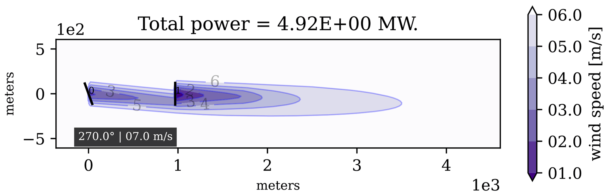
Figure 1 Example of WFFC on a two-turbine wind farm with the wind coming from the west. The first (upstream) turbine is misaligned and its wake effect is steered away from the second (downstream) turbine. By letting the wind flow more freely to the second turbine, the misalignment of the first turbine increases the total power output of the farm.

Current implemented wake steering strategies usually involve lookup tables (LUTs) (Fleming et al., 2017; Siemens Gamesa Renewable Energy, 2019). Wake steering strategies are computed for a finite set of different wind conditions prior to the farm operation. The yaw angles of each turbine are computed with steady-state models, regardless of the wind and turbine dynamics. Because a wake steering strategy creates misalignment with the wind, it is highly dependent on variations in the direction of the wind. The wind direction can change over time, and yaw control is constrained by the limited rotational speed of the nacelles. If the wind varies in directions and frequencies that the yaw actuators cannot easily track, computing adequate wake steering strategies over time can be a challenging task.

1.2 Wind direction dynamics

The study of wind direction dynamics is gaining interest within the research community. Wind direction dynamics can be broken down into large-scale drifts and small-scale fluctuations (van Doorn et al., 2000) and can be observed on different scales: the synoptic scale describes long distances and extended time periods, the mesoscale depicts the farm level and time periods from days to weeks, and the microscale corresponds to the turbine level and variations from seconds to minutes. The wind direction is fundamentally nonstationary, and there is incomplete knowledge regarding the physical and statistical characteristics of wind direction fluctuations across specific length scales and timescales that are essential for effective WFFC (Dallas et al., 2024).

As the farm operates, the wind direction varies in both time (at the farm level) and space (at the turbine level). The study by von Brandis et al. (2023) found that spatial wind direction changes relevant to the operation of wind farm clusters in the German Bight exceed 11° in 50 % of cases. In this present work, numerical simulations are run with steady-state wake models. Therefore, only variations in the wind at the farm level are studied. When the direction varies over time, this work considers it to affect the whole wind farm.

WFFC is most beneficial at low wind speeds because this is where small changes in the wind speeds can lead to important power output variations. The same wake steering strategy will lead to higher power gains at low speeds compared to higher wind speed. Because the wind direction variability is higher for low wind speeds (von Brandis et al., 2023; van Doorn et al., 2000; Dallas et al., 2024), the study of dependence between wind direction variations and yaw control is important. Also, because the impact of climate change on wind dynamics is unknown, designing robust controllers is necessary for long-term operation.

1.3 Related works

As tracking wind direction is essential for wind turbines, the literature is rich in studies seeking better wind direction tracking mechanisms. Song et al. (2018) developed a model predictive control (MPC)-based controller on a finite control set to track the wind directions. Hure et al. (2015) designed a yaw controller based on very short-term wind predictions. But performing WFFC and wake steering is a more complex optimization problem.

LUTs can be adapted for dynamic control with different methods. Usually, a low-pass filter is used to apply control only for high variations of the direction. A sampling method can be used to adjust the yaw control frequency, and hysteresis mechanisms avoid unnecessary yaw control and restrict the yaw actuators (Kanev, 2020a). Simley et al. (2021) improved a traditional LUT by anticipating the wind direction changes ahead of upstream turbines. Kanev (2020b) performed WFFC with a receding horizon using gradient-based optimization and ran tests in large-eddy simulations under realistic variations in wind direction and speed. But the wake steering strategies of an LUT fundamentally do not consider the wind dynamics; only their implementation does.

Regarding machine learning (ML) methods, and more particularly reinforcement learning (RL), which is becoming a source of great interest to the scientific community, wind direction variations are often overlooked. The importance of the wind direction dynamics is clearly pointed out by Saenz-Aguirre et al. (2019) and Saenz-Aguirre et al. (2020), but most of the studies carried out later only consider static or quasi-static wind directions. Some recent works have started to consider time-varying wind directions in WFFC optimization (Kadoche et al., 2023).

1.4 Contributions

The remainder of this paper is structured to mirror the three main contributions. Each contribution forms the basis of an individual section, and Sect. 5 concludes. The contributions and their corresponding sections are as follows.

• This work proposes a discretized formalization of the WFFC problem over time as the succession of multiple steady-state optimization problems interconnected by the rotational constraints of the turbines and the evolution of the wind. Due to the discretization hypothesis and the yaw actuation constraints, the important hypotheses regarding the transition between one steady state and the next are formulated. This formalization is conducted in Sect. 2.

• To develop a prediction-based controller, this work presents a reformulation of the instantaneous, steady-state original sequential decision problem over a future time window. The default objective function is augmented by a new heuristic, computed on a prediction of the wind. The proposed heuristic acts as a penalization for the optimization without increasing its dimension and encourages solutions that will guarantee future energy production. The heuristic and the other studied controllers are detailed in Sect. 3.

• This work conducts a sensitivity analysis of the wind direction variations and wake steering optimization. It empirically demonstrates the importance of a wind-prediction-based control when the magnitude of the wind direction fluctuations becomes large. The new proposed heuristic greatly improves the performance of a traditional steady-state wake steering optimization when the variations of the wind direction are important. Numerical simulations using synthetic wind data are conducted in Sect. 4.

2 Problem formalization

The environment is composed of a wind farm and some exogenous variables related to the wind direction and the wind speed. The wind farm consists of N interconnected wind turbines. Over time, each turbine is controlled via its yaw. An episode consists of a succession of H time steps during which the turbines are controlled, with H the horizon length. The transition from a time step t to a time step t+1 corresponds to a specific time window of a constant length of Δt minutes. The environment evolves from one time step t to the next time step t+1 in Δt minutes, with $t\in \mathit{\{}\mathrm{0},\mathrm{1},\mathrm{\dots },H-\mathrm{1}\mathit{\}}$.

2.1 Wind data

At a time step t, the exogenous variables are a global incoming wind direction $K_t\in [\mathrm{0},\mathrm{360}]$ [°] and a global incoming wind speed $V_t\in [{\mathit{\nu }}_{\text{min}},{\mathit{\nu }}_{\text{max}}]$ [m s⁻¹]. The wind data can be measured or predicted. Then, a controller does not have access to K_t and V_t directly but to $K_t^{\prime }$ [°] and $V_t^{\prime }$ [m s⁻¹], with $K_t^{\prime }$ a noisy wind direction defined as $K_t^{\prime }=K_t+{\mathit{ϵ}}_{K,t}$, and $V_t^{\prime }$ is a noisy wind speed defined as $V_t^{\prime }=V_t+{\mathit{ϵ}}_{V,t}$. The random noises ϵ_K,t and ϵ_V,t can come from either measurement imprecisions or prediction errors.

Because the turbines alter the wind flow inside the farm, the wind in front of a turbine can be different from the global incoming wind. Then, at a time step t, in front of a turbine i, the local wind direction is denoted as ${\mathit{\kappa }}_t^i$ [°] and the local wind speed is denoted as ${\mathit{\nu }}_t^i$ [m s⁻¹]. The computation of the local velocities is based on complex fluid mechanics and is subject to numerous uncertainties. This work conducts numerical experiments where such computations are done using a low-fidelity, steady-state simulator: FLOw Redirection and Induction in Steady State (FLORIS) NREL (2021). The local wind directions stay equal to the global wind direction for any time step, i.e., ${\mathit{\kappa }}_t^i=K_t\forall i\in \mathit{\{}\mathrm{0},\mathrm{1},\mathrm{\dots },N-\mathrm{1}\mathit{\}}$, as is common for low-fidelity, steady-state simulations.

2.2 Turbines

At a time step t, a turbine i is characterized by its absolute angular position ${\mathit{\beta }}_t^i\in [\mathrm{0},\mathrm{360}]$ [°] and its relative orientation or yaw (often used to compute the power output) ${\mathit{\alpha }}_t^i=f_{\text{yaw}}(K_t,{\mathit{\beta }}_t^i)\in [-\mathrm{180},\mathrm{180}]$ [°] such that

$$\begin{array}{}\text{(1)}& f_{\text{yaw}}(K_t,{\mathit{\beta }}_t^i)=(K_t-{\mathit{\beta }}_t^i+\mathrm{180})\mathrm{mod}\mathrm{360}-\mathrm{180}.\end{array}$$

Adding and subtracting by 180 ensures that the yaw stays in the range $[-\mathrm{180},\mathrm{180}]$. As illustrated in Fig. 2, the yaw corresponds to the rotational movement going from the absolute angular position ${\mathit{\beta }}_t^i$ to the wind direction K_t such that ${\mathit{\beta }}_t^i+{\mathit{\alpha }}_t^i\mathrm{mod}\mathrm{360}=K_t$. Positive values of the yaw indicate that the turbine is rotated anticlockwise from the wind direction, and negative values of the yaw indicate that the turbine is rotated clockwise from the wind direction.

At a time step t, the yaw setting $u_t^i\in [u_{\text{min}},u_{\text{max}}]$ [°] of a turbine i corresponds to the rotational movement of the turbine between time steps t and t+1. Because of mechanical constraints related to the yaw actuator of the nacelle, the yaw setting is bounded between two consecutive time steps. As illustrated in Fig. 2, the setting is used to update the orientation of the turbine ${\mathit{\beta }}_{t+\mathrm{1}}^i=f_{\text{control}}({\mathit{\beta }}_t^i,u_t^i)$ such that

$$\begin{array}{}\text{(2)}& f_{\text{control}}({\mathit{\beta }}_t^i,u_t^i)=({\mathit{\beta }}_t^i+u_t^i)\mathrm{mod}\mathrm{360}.\end{array}$$

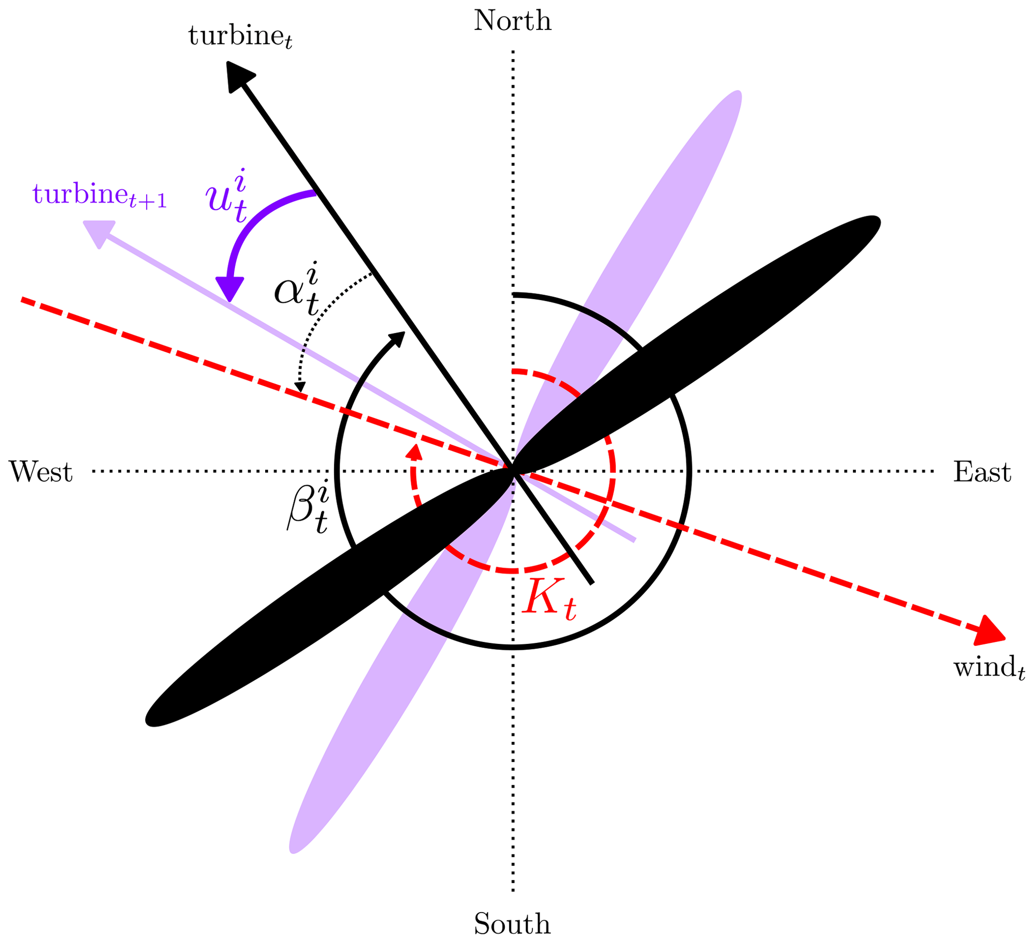
Figure 2 Example of a wind turbine i seen from above at a time step t. The variables are the wind direction K_t, the absolute angular position ${\mathit{\beta }}_t^i$ of the turbine, and the yaw ${\mathit{\alpha }}_t^i$ of the turbine. The wind direction indicates where the wind is coming from; e.g., a wind direction of 270° indicates a wind coming from the west. Here, the nacelle is misaligned with the incoming wind direction: the turbine is rotated clockwise from the wind, so ${\mathit{\alpha }}_t^i<\mathrm{0}$. The yaw setting $u_t^i$ gives the next orientation of the turbine at time step t+1.

2.3 Power

The power curve Φ of a turbine gives the theoretical power output (megawatts, MW; y axis) of the machine as a function of the wind speed ν [m s⁻¹] (x axis), considering no yaw misalignment, such that

$$\begin{array}{}\text{(3)}& \mathrm{\Phi }\left(\mathit{\nu }\right)={\displaystyle \frac{\mathrm{1}}{\mathrm{2}}}\cdot \mathit{\rho }\cdot A\cdot {\mathit{\nu }}^{\mathrm{3}}\cdot C_{\mathrm{P}}\left(\mathit{\nu }\right),\end{array}$$

with ρ [kg m⁻³] the air density, A [m²] the rotor blade area, and C_P the power coefficient of the turbine. The theoretical power output is strictly positive if the wind speed is within certain bounds [ν_cut-in,ν_cut-out] [m s⁻¹].

At a time step t, the power output of a turbine i considering yaw misalignment $P_t^i=f_{\text{power}}({\mathit{\nu }}_t^i,{\mathit{\alpha }}_t^i)$ [MW] is computed from the power curve and the yaw angle such that

$$\begin{array}{}\text{(4)}& f_{\text{power}}({\mathit{\nu }}_t^i,{\mathit{\alpha }}_t^i)=\mathrm{\Phi }\left({\mathit{\nu }}_t^i\right)\cdot {\cos }^p\left({\mathit{\alpha }}_t^i\right)\cdot {\text{𝟙}}_{\mathit{\{}{\mathit{\alpha }}_{\text{cut-in}}⩽{\mathit{\alpha }}_t^i⩽{\mathit{\alpha }}_{\text{cut-out}}\mathit{\}}},\end{array}$$

with p a parameter accounting for power losses due to misalignment and [α_cut-in,α_cut-out] [°] a safety bound for the yaw taken into account by the indicator function. Because too much misalignment with the wind can damage the machine, if the yaw is too great, the turbine is shut down and its power output is null.

2.4 Policy

A policy π is a function returning the yaw settings $(u_t^{\mathrm{0}},u_t^{\mathrm{1}},\mathrm{\dots },u_t^{N-\mathrm{1}})$ of all the turbines at a time step t given a state s_t. Each wind farm controller is associated with a specific policy. In this work, the state s_t may be composed of

• the current orientations of the turbines $\mathit{\{}{\mathit{\beta }}_t^i{\mathit{\}}}_{i\in \mathit{\{}\mathrm{0},\mathrm{1},\mathrm{\dots },N-\mathrm{1}\mathit{\}}}$,

• an observation of the current wind $(K_t^{\prime },V_t^{\prime })$,

• a prediction of the wind at time step t+1 $(K_{t+\mathrm{1}}^{\prime },V_{t+\mathrm{1}}^{\prime })$,

• a prediction of the wind at time step t+2 $(K_{t+\mathrm{2}}^{\prime },V_{t+\mathrm{2}}^{\prime })$, and

• until time step t+L, with L the prediction horizon.

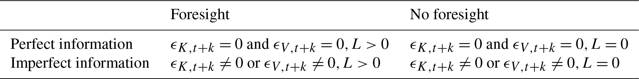
Therefore, the general form of a state is $s_t=\mathit{\{}{K}_t^{\prime },V_t^{\prime },K_{t+\mathrm{1}}^{\prime },V_{t+\mathrm{1}}^{\prime },\mathrm{\dots },K_{t+L}^{\prime },V_{t+L}^{\prime },\mathit{\{}{\mathit{\beta }}_t^i{\mathit{\}}}_{i\in \mathit{\{}\mathrm{0},\mathrm{1},\mathrm{\dots },N-\mathrm{1}\mathit{\}}}\mathit{\}}$. States can be categorized based on two distinct properties: with perfect or imperfect information and with or without foresight knowledge. Depending on the possible combinations, there are four classes of states, listed in Table 1.

Table 1 Four different classes of states based on two distinct properties, with $t\in \mathit{\{}\mathrm{0},\mathrm{1},\mathrm{\dots },H-\mathrm{1}\mathit{\}}$ and $k\in \mathit{\{}\mathrm{0},\mathrm{1},\mathrm{\dots },L\mathit{\}}$. With perfect information, the state comprises exact wind data (no noise). Without foresight, the state only comprises the current wind data (no predictions).

2.5 System evolution

An episode is defined by H time steps during which turbines are controlled via their yaw. An episode is characterized by time series for the wind directions and the wind speeds as well as initial positions for the nacelles. During an episode, it is assumed that all the states belong to the same class (defined in Table 1) and the policy is presumed to be stationary (it does not change over time).

The full evolution of an episode is described in Algorithm (1). At each time step, the policy returns the yaw settings based on the current state, the system is updated, and the power output of the farm is computed. The yaw setting of a turbine i at the end of time step t is indexed t+1 (because it has been updated) and it is the one used for the power computation of time step t.

Algorithm 1 Full episode evolution over time.

Input: $\mathit{\{}{K}_k,V_k{\mathit{\}}}_{k\in \mathit{\{}\mathrm{0},\mathrm{1},\mathrm{\dots },H+L-\mathrm{1}\mathit{\}}}$ true wind data time series

$\mathit{\{}{\mathit{\beta }}_{\mathrm{0}}^i{\mathit{\}}}_{i\in \mathit{\{}\mathrm{0},\mathrm{1},\mathrm{\dots },N-\mathrm{1}\mathit{\}}}$ initial orientations

π yaw control policy

for $t=\mathit{\{}\mathrm{0},\mathrm{1},\mathrm{\dots },H-\mathrm{1}\mathit{\}}$ do

$s_t=\mathit{\{}{K}_t^{\prime },V_t^{\prime },K_{t+\mathrm{1}}^{\prime },V_{t+\mathrm{1}}^{\prime },\mathrm{\dots },K_{t+L}^{\prime },V_{t+L}^{\prime },\mathit{\{}{\mathit{\beta }}_t^i{\mathit{\}}}_{i\in \mathit{\{}\mathrm{0},\mathrm{1},\mathrm{\dots },N-\mathrm{1}\mathit{\}}}\mathit{\}}$

▹ state

$(u_t^{\mathrm{0}},u_t^{\mathrm{1}},\mathrm{\dots },u_t^{N-\mathrm{1}})=\mathit{\pi }\left(s_t\right)$

▹ control policy

${\mathit{\beta }}_{t+\mathrm{1}}^i=f_{\text{control}}({\mathit{\beta }}_t^i,u_t^i),\forall i\in \mathit{\{}\mathrm{0},\mathrm{\dots },N-\mathrm{1}\mathit{\}}$

▹ angular positions update

${\mathit{\alpha }}_{t+\mathrm{1}}^i=f_{\text{yaw}}(K_t,{\mathit{\beta }}_{t+\mathrm{1}}^i),\forall i\in \mathit{\{}\mathrm{0},\mathrm{\dots },N-\mathrm{1}\mathit{\}}$

▹ yaw angles computation

${\mathit{\nu }}_t^i=f_{\text{simulation}}^i(K_t,V_t,\mathit{\{}{\mathit{\alpha }}_{t+\mathrm{1}}^j{\mathit{\}}}_{j\in \mathit{\{}\mathrm{0},\mathrm{1},\mathrm{\dots },N-\mathrm{1}\mathit{\}}}),\forall i\in \mathit{\{}\mathrm{0},\mathrm{\dots },N-\mathrm{1}\mathit{\}}$

▹ local velocities computation

$P_t^i=f_{\text{power}}({\mathit{\nu }}_t^i,{\mathit{\alpha }}_{t+\mathrm{1}}^i),\forall i\in \mathit{\{}\mathrm{0},\mathrm{\dots },N-\mathrm{1}\mathit{\}}$

▹ power outputs computation

end for

Output: ${\sum }_{t=\mathrm{0}}^{H-\mathrm{1}}{\sum }_{i=\mathrm{0}}^{N-\mathrm{1}}{P}_t^i$ farm power output

At a time step t, to compute the power output of each turbine, local wind velocities are needed. Such computations rely on complex fluid mechanics, depending on the incoming wind and the updated yaw angles of each turbine. For optimization, performing such complex computations is computationally expensive. Therefore, in this work, these computations are carried out by a steady-state simulator ${\mathit{\nu }}_t^i=f_{\text{simulation}}^i(K_t,V_t,\mathit{\{}{\mathit{\alpha }}_{t+\mathrm{1}}^j{\mathit{\}}}_{j\in \mathit{\{}\mathrm{0},\mathrm{1},\mathrm{\dots },N-\mathrm{1}\mathit{\}}})$, which is used as a substitute for real-life measurements.

The simulation is said to be steady-state because it only depends on the current global wind data and the updated yaw angles. It does not consider previous wind data, previous yaw angles, or time delays in the wake propagation. The evolution of an episode over time is constrained by the rotational bounds of the turbines and the variations of the wind.

At each time step, during the “control policy” operation, a controller knows the evolution mechanisms of the system; i.e., it can conduct any computations with the $f_{\text{control}},f_{\text{yaw}},f_{\text{simulation}}^i$, and f_power functions but based on the wind data provided by the state. Because such data can be noisy, all the computed values can be inexact. For example, at a time step t, if a controller computes the yaw of a turbine i based on its updated orientation ${\mathit{\beta }}_{t+\mathrm{1}}^i$, it would be equal to ${{\mathit{\alpha }}_{t+\mathrm{1}}^i}^{\prime }=f_{\text{yaw}}(K_t^{\prime },{\mathit{\beta }}_{t+\mathrm{1}}^i)$. Because the observed wind direction $K_t^{\prime }$ can be different from the true wind direction K_t, the yaw ${{\mathit{\alpha }}_{t+\mathrm{1}}^i}^{\prime }$ estimated by a controller can be different from its true value ${\mathit{\alpha }}_{t+\mathrm{1}}^i$.

2.6 Transition regime

At a time step t, for a turbine i, and due to the steady-state nature of the simulation, the WFFC problem thus formalized considers a single power output $P_t^i$. In reality, during a time step, the wind is time-varying and a turbine takes time to rotate because of mechanical constraints. Therefore, the discretization of the continuous control problem results in the loss of some information and possibly less inaccurate power outputs. To ensure that the discretized power outputs are good approximations, from one time step to another, a turbine is assumed to rotate immediately and the wind is assumed to be quasi-constant.

The duration of a time step is always considered constant during an episode. At a time step t, when a setting $u_t^i$ is applied to a turbine i, the rotational time T_r (minutes) for the turbine to go from its current orientation ${\mathit{\beta }}_t^i$ to its next orientation ${\mathit{\beta }}_{t+\mathrm{1}}^i$ is always considered largely inferior to the duration of the time step, i.e., T_r≪Δt for all $u_t^i\in [u_{\text{min}},u_{\text{max}}]$. A turbine always rapidly reaches its target position before the end of the time step duration. But during a time step, no other control will be applied to the turbine. For this reason, the rotational constraints [u_min,u_max] need to be consistent with the duration of a time step Δt.

The coherence time T_c (minutes) of a wind variable (either the direction or the speed) is the maximum duration during which the variable is quasi-constant. If the coherence time of the wind direction is strictly smaller than the time step duration, a discretized value K_t would stretch too far away from its corresponding continuous signal. The same goes for the speed. Therefore, in this work, the coherence time is always equal to the time step duration, i.e., T_c=Δt, for both the direction and the speed.

3 Controllers

At a time step t, the yaw settings $(u_t^{\mathrm{0}},u_t^{\mathrm{1}},\mathrm{\dots },u_t^{N-\mathrm{1}})$ are denoted as u_t. A controller is defined by its policy π(s_t) with the state s_t described in Sect. 2.4. This work compares a naive control where each turbine is aligned as much as possible with the wind and three optimized wake steering control strategies. In an episode, at each time step t, during the control policy operation of Algorithm (1), each controller computes the yaw settings such that u_t=π(s_t) by maximizing a specific objective function f_obj(s_t,u_t) with regard to the turbine rotational constraints, as defined below.

$$\begin{array}{}\text{(5)}& {\displaystyle }\mathit{\pi }\left(s_t\right)\in \underset{u_t}{\arg max}{f}_{\text{obj}}(s_t,u_t),\text{(6)}& {\displaystyle }\begin{array}{rl}& \text{subject to}{u}_{\text{min}}⩽u_t^i⩽u_{\text{max}},\\ & \forall t\in \mathit{\{}\mathrm{0},\mathrm{1},\mathrm{\dots },H-\mathrm{1}\mathit{\}},\forall i\in \mathit{\{}\mathrm{0},\mathrm{1},\mathrm{\dots },N-\mathrm{1}\mathit{\}}.\end{array}\end{array}$$

3.1 Naive controller

The naive controller always tries to keep turbines aligned with the current wind direction as much as possible. It is a weak baseline as it does not conduct any wake steering optimization. It runs with no foresight (i.e., L=0), as it is only concerned with the current observed wind direction $K_t^{\prime }$. Therefore, the state s_t is reduced to $\mathit{\{}{K}_t^{\prime },\mathit{\{}{\mathit{\beta }}_t^i{\mathit{\}}}_{i\in \mathit{\{}\mathrm{0},\mathrm{1},\mathrm{\dots },N-\mathrm{1}\mathit{\}}}\mathit{\}}$. It consists of a greedy control (no wake steering) where the objective function at a time step t minimizes the amplitude of the yaws, i.e.,

$$\begin{array}{}\text{(7)}& {\displaystyle }{f}_{\text{obj}}(s_t,u_t)=-\sum _{i=\mathrm{0}}^{N-\mathrm{1}}\left|{{\mathit{\alpha }}_{t+\mathrm{1}}^i}^{\prime }\right|,\text{(8)}& {\displaystyle }\text{with}{{\mathit{\alpha }}_{t+\mathrm{1}}^i}^{\prime }=f_{\text{yaw}}(K_t^{\prime },{\mathit{\beta }}_{t+\mathrm{1}}^i),\text{(9)}& {\displaystyle }\text{with}{\mathit{\beta }}_{t+\mathrm{1}}^i=f_{\text{control}}({\mathit{\beta }}_t^i,u_t^i).\end{array}$$

At a time step t, the rotational movement required for a turbine i to stay aligned with the observed wind direction is equal to $f_{\text{yaw}}(K_t^{\prime },{\mathit{\beta }}_t^i)$. Because of the rotational constraints, this movement is clipped such that it is always an acceptable setting with regards to the yaw actuator, giving a closed-form expression for the solution, defined as

$$\begin{array}{}\text{(10)}& {\displaystyle }{\mathit{\pi }}_{\text{naive}}=(u_t^{\mathrm{0}},u_t^{\mathrm{1}},\mathrm{\dots },u_t^{N-\mathrm{1}}),\text{(11)}& {\displaystyle }\begin{array}{rl}& \text{such that}{u}_t^i=\text{clip}\left(f_{\text{yaw}}\right(K_t^{\prime },{\mathit{\beta }}_t^i),u_{\text{min}},u_{\text{max}}),\\ & \forall i\in \mathit{\{}\mathrm{0},\mathrm{1},\mathrm{\dots },N-\mathrm{1}\mathit{\}}.\end{array}\end{array}$$

3.2 Wake steering

Compared to naive control, wake steering is used to optimize the power output of the farm. In this work, two distinct wake steering strategies are used. One is based only on the instantaneous wind data, and one is based on instantaneous and predicted wind data. The instantaneous controller searches for the yaw settings maximizing the instantaneous power output of the farm. The prediction-based controller maximizes the instantaneous and future power outputs. At each time step t, the same Gauss–Seidel (GS) method is used for both controllers, but with different objective functions. In this work, optimization is conducted with a GS method (described in Algorithm A1). A similar approach was first proposed by Fleming et al. (2022) with a serial-refine algorithm.

The GS method works as follows. A first solution is initialized from the naive controller, where each initial yaw setting keeps its turbine aligned as much as possible with the wind. Then, the GS method iterates over each turbine, from upstream to downstream ones. At each iteration, it solves the optimization problem for the current turbine, considering the yaw settings of all others fixed, by conducting a grid search over a discretized solution space $S=\mathit{\{}{u}_{\text{min}}+l\cdot \frac{u_{\text{max}}-u_{\text{min}}}{n_y-\mathrm{1}}\mathit{\}}$ for all $l\in \mathit{\{}\mathrm{0},\mathrm{1},\mathrm{\dots },n_y-\mathrm{1}\mathit{\}}$, with n_y being a precision parameter. Once optimized, the setting of the current turbine is updated, and it goes to the next one.

3.2.1 Instantaneous controller

The instantaneous controller searches for the yaw settings maximizing the immediate power output of the farm. It always runs under no foresight (i.e., L=0), as it performs wake steering for the current observed wind data only. Therefore, the state s_t is reduced to $\mathit{\{}{K}_t^{\prime },V_t^{\prime },\mathit{\{}{\mathit{\beta }}_t^i{\mathit{\}}}_{i\in \mathit{\{}\mathrm{0},\mathrm{1},\mathrm{\dots },N-\mathrm{1}\mathit{\}}}\mathit{\}}$. It is a steady-state optimization performed on one time step where the objective function at a time step t is the immediate normalized power output, i.e.,

$$\begin{array}{}\text{(12)}& {\displaystyle }{f}_{\text{obj}}(s_t,u_t)={\displaystyle \frac{\mathrm{1}}{N}}\cdot \sum _{i=\mathrm{0}}^{N-\mathrm{1}}{f}_{\text{power}}({{\mathit{\nu }}_t^i}^{\prime },{{\mathit{\alpha }}_{t+\mathrm{1}}^i}^{\prime }),\text{(13)}& {\displaystyle }\text{with}{{\mathit{\nu }}_t^i}^{\prime }=f_{\text{simulation}}^i(K_t^{\prime },V_t^{\prime },\mathit{\{}{{\mathit{\alpha }}_{t+\mathrm{1}}^j}^{\prime }{\mathit{\}}}_{j\in \mathit{\{}\mathrm{0},\mathrm{1},\mathrm{\dots },N-\mathrm{1}\mathit{\}}}),\text{(14)}& {\displaystyle }\text{with}{{\mathit{\alpha }}_{t+\mathrm{1}}^i}^{\prime }=f_{\text{yaw}}(K_t^{\prime },{\mathit{\beta }}_{t+\mathrm{1}}^i),\text{(15)}& {\displaystyle }\text{with}{\mathit{\beta }}_{t+\mathrm{1}}^i=f_{\text{control}}({\mathit{\beta }}_t^i,u_t^i).\end{array}$$

3.2.2 Prediction-based controller

A traditional prediction-based controller searches for the yaw settings of time steps $t,t+\mathrm{1},\mathrm{\dots },t+L$ that maximize the power output over that horizon. It always runs with foresight (i.e., L⩾1). The corresponding sequential decision problem over a future time window can be stated under a form usually exploited by the MPC community, defined as

$$\begin{array}{}\text{(16)}& {\displaystyle }\underset{u_t,u_{t+\mathrm{1}},\mathrm{\dots },u_{t+L}}{max}{\displaystyle \frac{\mathrm{1}}{N}}\cdot \sum _{k=\mathrm{0}}^L\sum _{i=\mathrm{0}}^{N-\mathrm{1}}{f}_{\text{power}}({{\mathit{\nu }}_{t+k}^i}^{\prime },{{\mathit{\alpha }}_{t+k+\mathrm{1}}^i}^{\prime }),\text{(17)}& {\displaystyle }\begin{array}{rl}& \text{subject to}{u}_{\text{min}}⩽u_{t+k}^i⩽u_{\text{max}},\forall t\in \mathit{\{}\mathrm{0},\mathrm{1},\mathrm{\dots },H-\mathrm{1}\mathit{\}},\\ & \forall k\in \mathit{\{}\mathrm{0},\mathrm{1},\mathrm{\dots },L\mathit{\}},\forall i\in \mathit{\{}\mathrm{0},\mathrm{1},\mathrm{\dots },N-\mathrm{1}\mathit{\}},\end{array}\text{(18)}& {\displaystyle }\begin{array}{rl}& \text{with}{{\mathit{\nu }}_{t+k}^i}^{\prime }=f_{\text{simulation}}^i\\ & (K_{t+k}^{\prime },V_{t+k}^{\prime },\mathit{\{}{{\mathit{\alpha }}_{t+k+\mathrm{1}}^j}^{\prime }{\mathit{\}}}_{j\in \mathit{\{}\mathrm{0},\mathrm{1},\mathrm{\dots },N-\mathrm{1}\mathit{\}}}),\end{array}\text{(19)}& {\displaystyle }\text{with}{{\mathit{\alpha }}_{t+k+\mathrm{1}}^i}^{\prime }=f_{\text{yaw}}(K_{t+k}^{\prime },{\mathit{\beta }}_{t+k+\mathrm{1}}^i),\text{(20)}& {\displaystyle }\text{with}{\mathit{\beta }}_{t+k+\mathrm{1}}^i=f_{\text{control}}({\mathit{\beta }}_{t+k}^i,u_{t+k}^i).\end{array}$$

The optimization problem thus described multiplies the number of decision variables by L+1. Also, the computation of the local velocities at a given time step depends on all the previous yaw settings. Therefore, the prediction-based decision problem significantly increases the complexity, and because there is no simple solution, this work proposes a reformulation. The objective function given by Eq. (16) can be split between the current time step t and the next ones, from t+1 to t+L, such that

$$\begin{array}{}\text{(21)}& \begin{array}{rl}& {\displaystyle \frac{\mathrm{1}}{N}}\cdot \sum _{k=\mathrm{0}}^L\sum _{i=\mathrm{0}}^{N-\mathrm{1}}{f}_{\text{power}}({{\mathit{\nu }}_{t+k}^i}^{\prime },{{\mathit{\alpha }}_{t+k+\mathrm{1}}^i}^{\prime })=\underset{\text{first term}}{\underbrace{{\displaystyle \frac{\mathrm{1}}{N}}\cdot f_{\text{power}}({{\mathit{\nu }}_t^i}^{\prime },{{\mathit{\alpha }}_{t+\mathrm{1}}^i}^{\prime })}}\\ & +\underset{\text{second term}}{\underbrace{{\displaystyle \frac{\mathrm{1}}{N}}\cdot \sum _{k=\mathrm{1}}^L\sum _{i=\mathrm{0}}^{N-\mathrm{1}}{f}_{\text{power}}({{\mathit{\nu }}_{t+k}^i}^{\prime },{{\mathit{\alpha }}_{t+k+\mathrm{1}}^i}^{\prime })}}.\end{array}\end{array}$$

The first term of Eq. (21) is the normalized power output of the farm for the current time step. It corresponds to the objective function of the instantaneous controller defined in Sect. 3.2.1. It only depends on the current yaw settings u_t. Now, focusing on the second term, the closed-form expression of the f_power is written, giving

$$\begin{array}{}\text{(22)}& \begin{array}{rl}& {\displaystyle \frac{\mathrm{1}}{N}}\cdot \sum _{k=\mathrm{1}}^L\sum _{i=\mathrm{0}}^{N-\mathrm{1}}{f}_{\text{power}}({{\mathit{\nu }}_{t+k}^i}^{\prime },{{\mathit{\alpha }}_{t+k+\mathrm{1}}^i}^{\prime })=\\ & {\displaystyle \frac{\mathrm{1}}{N}}\cdot \sum _{k=\mathrm{1}}^L\sum _{i=\mathrm{0}}^{N-\mathrm{1}}\mathrm{\Phi }\left({{\mathit{\nu }}_{t+k}^i}^{\prime }\right)\cdot {\cos }^p\left({{\mathit{\alpha }}_{t+k+\mathrm{1}}^i}^{\prime }\right)\\ & \cdot {\text{𝟙}}_{\mathit{\{}{\mathit{\alpha }}_{\text{cut-in}}⩽{{\mathit{\alpha }}_{t+k+\mathrm{1}}^i}^{\prime }⩽{\mathit{\alpha }}_{\text{cut-out}}\mathit{\}}}.\end{array}\end{array}$$

The complexity brought by the prediction-based controller comes from the fact that Eq. (22) depends on the local velocities ${{\mathit{\nu }}_{t+k}^i}^{\prime }$ and the updated yaw angles ${{\mathit{\alpha }}_{t+k+\mathrm{1}}^i}^{\prime }$ corresponding to the optimized yaw settings of each future time step. To decrease the complexity, this work proposes modifying Eq. (22) in the following way.

• Each local velocity ${{\mathit{\nu }}_{t+k}^i}^{\prime }$ is replaced by the corresponding predicted global wind speed $V_{t+k}^{\prime }$. It reduces the complexity coming from the steady-state simulation by removing the dependence on the updated yaw angles. While this simplification removes future local wind data, it retains some information regarding potential future energy production by relying on the predicted global wind data only.

• Each updated yaw angle ${{\mathit{\alpha }}_{t+k+\mathrm{1}}^i}^{\prime }$ depending on the optimized yaw setting $u_{t+k}^i$ is replaced by the expected yaw angle ${\widehat{\mathit{\alpha }}}_{t+k+\mathrm{1}}^i{}^{\prime }$ if a naive controller was used instead. It reduces the complexity coming from the optimization, as there is a closed-from expression for the naive controller, as provided by Eq. (10). Replacing the wake steering optimization performed in the future with a naive wind tracking solution reduces the number of optimization variables of the original problem while keeping good solutions. Indeed, proper yaw settings are known to be close to the wind on average.

• The cosine function at power p of each yaw angle is replaced with a simpler penalization for yaw misalignment. The penalization chosen corresponds to 1 minus the normalized absolute value of that yaw angle. It provides linearity and better interpretability.

• The indicator function is removed so that there is no discontinuity. Even if a yaw is too great, it can be of some interest for the optimization to know about the potential power output. The more a turbine is misaligned, the less likely it will be to produce energy and the more it will be penalized.

• For each time step, the overall expression is multiplied by a discounted factor $\mathit{\gamma }\in [\mathrm{0},\mathrm{1}]$. It gives more importance to immediate time steps. It is common practice for model-predictive-based optimization.

The only variables specific to each turbine are the yaw angles updated from a naive controller, which are already normalized. Therefore, it becomes unnecessary to normalize the overall expression by N. With such modifications, Eq. (22) becomes a new heuristic ℋ_t defined as

$$\begin{array}{}\text{(23)}& {\displaystyle }\begin{array}{rl}& {\mathcal{H}}_t(s_t,u_t)=\sum _{k=\mathrm{1}}^L{\mathit{\gamma }}^{k-\mathrm{1}}\cdot \mathrm{\Phi }\left(V_{t+k}^{\prime }\right)\\ & \cdot \left(\mathrm{1}-{\displaystyle \frac{\mathrm{1}}{N}}\cdot {\displaystyle \frac{\mathrm{1}}{\mathrm{180}}}\cdot \sum _{i=\mathrm{0}}^{N-\mathrm{1}}\left|{\widehat{\mathit{\alpha }}}_{t+k+\mathrm{1}}^i{}^{\prime }\right|\right),\end{array}\text{(24)}& {\displaystyle }\text{with}{\widehat{\mathit{\alpha }}}_{t+k+\mathrm{1}}^i{}^{\prime }=f_{\text{yaw}}(K_{t+k}^{\prime },{\widehat{\mathit{\beta }}}_{t+k+\mathrm{1}}^i),\text{(25)}& {\displaystyle }\begin{array}{rl}& \text{with}{\widehat{\mathit{\beta }}}_{t+k+\mathrm{1}}^i=f_{\text{control}}({\widehat{\mathit{\beta }}}_{t+k}^i,{\widehat{u}}_{t+k}^i),\\ & {\widehat{u}}_{t+k}^i\text{computed with a naive controller}\\ & \text{defined by Eq. (10)},\end{array}\text{(26)}& {\displaystyle }\begin{array}{rl}& \text{with}{\widehat{\mathit{\beta }}}_{t+\mathrm{1}}^i=f_{\text{control}}({\mathit{\beta }}_t^i,u_t^i),u_t^i\text{computed from a wake}\\ & \text{steering optimization}.\end{array}\end{array}$$

Because this new proposed heuristic depends on neither the future optimized yaw settings (naive control) nor the future local velocities (no simulation), it does not increase the number of optimization variables. The heuristic is a scalar acting as a penalization for the optimization. The final objective function of the prediction-based controller can finally be written as

$$\begin{array}{}\text{(27)}& {\displaystyle }{f}_{\text{obj}}(s_t,u_t)={\displaystyle \frac{\mathrm{1}}{N}}\cdot \sum _{i=\mathrm{0}}^{N-\mathrm{1}}{f}_{\text{power}}({{\mathit{\nu }}_t^i}^{\prime },{{\mathit{\alpha }}_{t+\mathrm{1}}^i}^{\prime })+{\mathcal{H}}_t(s_t,u_t),\text{(28)}& {\displaystyle }\text{with}{{\mathit{\nu }}_t^i}^{\prime }=f_{\text{simulation}}^i(K_t^{\prime },V_t^{\prime },\mathit{\{}{{\mathit{\alpha }}_{t+\mathrm{1}}^j}^{\prime }{\mathit{\}}}_{j\in \mathit{\{}\mathrm{0},\mathrm{1},\mathrm{\dots },N-\mathrm{1}\mathit{\}}}),\text{(29)}& {\displaystyle }\text{with}{{\mathit{\alpha }}_{t+\mathrm{1}}^i}^{\prime }=f_{\text{yaw}}(K_t^{\prime },{\mathit{\beta }}_{t+\mathrm{1}}^i),\text{(30)}& {\displaystyle }\text{with}{\mathit{\beta }}_{t+\mathrm{1}}^i=f_{\text{control}}({\mathit{\beta }}_t^i,u_t^i),\text{(31)}& {\displaystyle }\text{with}{\mathcal{H}}_t(s_t,u_t)\text{defined by Eq. (23)}.\end{array}$$

The heuristic is the discounted weighted sum of the future theoretical power outputs. By choosing certain optimized yaw settings u_t for the current time step, the heuristic uses a naive controller over a future time horizon of L time steps to evaluate how well the turbines will manage to stay aligned with the predicted wind directions. The higher the potential future energy production, the more critical it becomes for the current yaw settings not to rotate the turbines too far away from the predicted wind direction.

For example, if the future expected power outputs are high, the heuristic will encourage yaw settings that will put the turbines in good orientations for the future. The heuristic will penalize the objective function for yaw settings that will prevent turbines from keeping track of the wind. An illustration of the heuristic is given in Fig. 3, describing the first term (wake steering optimization) and the second term (heuristic based on a wind tracking control) of Eq. (27).

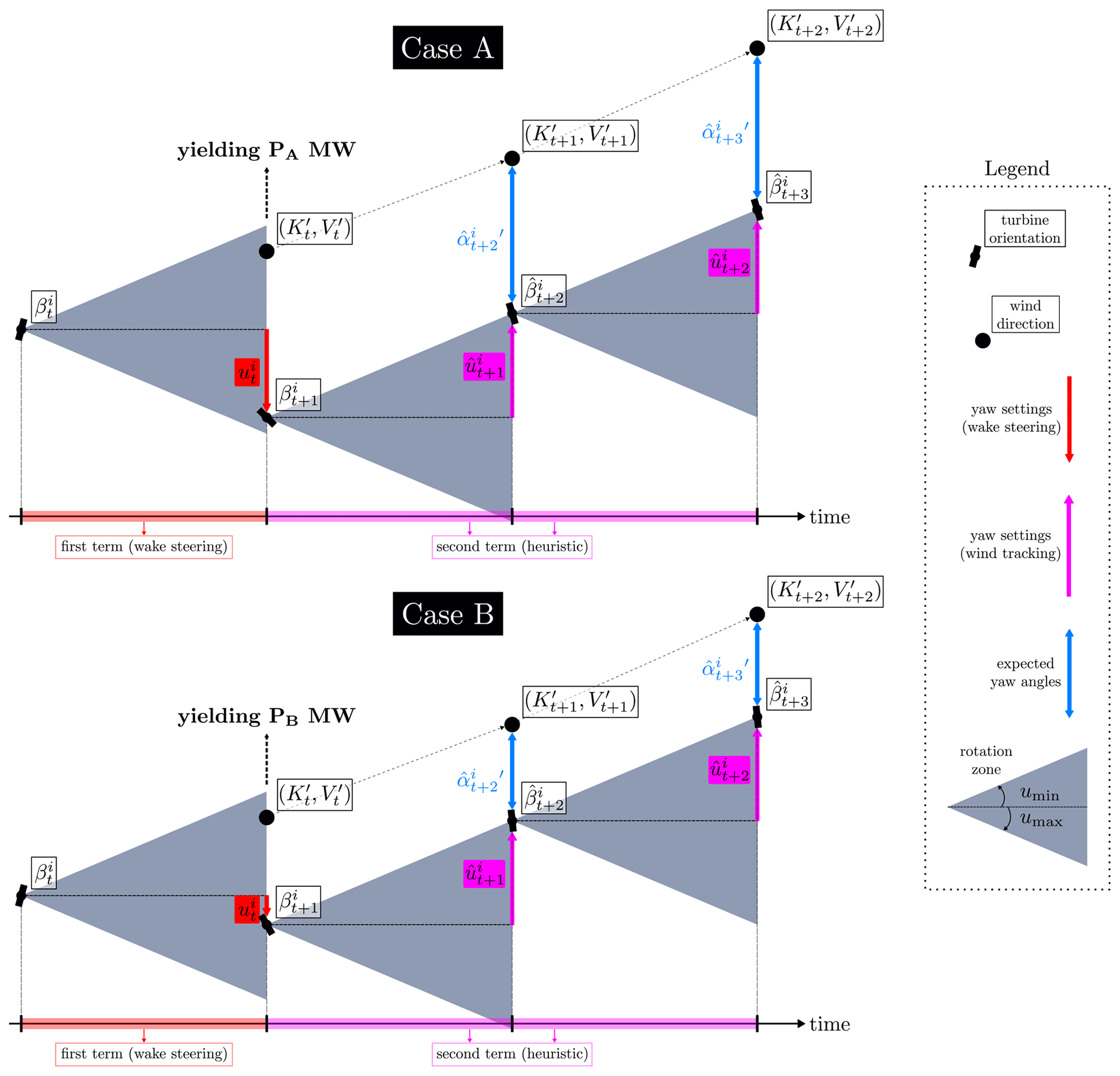
Figure 3 Illustration of the heuristic for a turbine i at time step t for two different cases. The horizon is L=2 and the wind data are the same for cases A and B. The rotation zone represents the range of possible orientations a turbine can take at a given time step after being controlled. First, wake steering optimization is performed to find the setting $u_t^i$, which yields a power output of P_A MW for case A and P_B MW for case B at time step t. By considering P_A>P_B, case A would be preferred. But then the heuristic computes the future expected yaw angles if a naive wind tracking solution is used. From these expected yaw angles, the heuristic computes the expected power outputs based on the predicted wind speeds. Here, while the yaw setting of case A gives a better immediate solution than the one given by case B, it keeps the turbine further away (i.e., giving greater yaw angles) from the future wind. The solution of case B would then be preferable. The heuristic encourages the choice of yaw settings that may not be the best at the current time step but that ensures future power output.

3.3 Upper bound

To have an upper bound in terms of performance (power output) of a wake steering strategy, the rotational constraints are relaxed. It means that in Eq. (6), the variables u_min and u_max are equal to −180 and 180°, respectively. Between two consecutive time steps, each turbine is assumed to be capable of reaching any orientation.

From a different point of view, the upper bound corresponds to the wake steering instantaneous controller, but for a complete steady-state version of the system evolution presented in Algorithm (1). All time steps are entirely independent from each other, as there are no longer any rotational constraints for the turbines.

The same objective function of the instantaneous controller, presented in Sect. 3.2.1, is used. It always runs under no foresight (i.e., L=0), as it performs wake steering for the current wind data only. Therefore, the state s_t is reduced to $\mathit{\{}{K}_t^{\prime },V_t^{\prime },\mathit{\{}{\mathit{\beta }}_t^i{\mathit{\}}}_{i\in \mathit{\{}\mathrm{0},\mathrm{1},\mathrm{\dots },N-\mathrm{1}\mathit{\}}}\mathit{\}}$. The yaw settings computed by the upper bound would not be admissible in reality if the corresponding targeted orientations are too far away from the current ones.

4 Simulations

In Sect. 4.1 the process used to generate wind data is described, and in Sect. 4.2 the experiment setting is given. Finally, the results and the empirical conclusions that can be drawn are explained in Sect. 4.3.

4.1 Wind data scenario

The wind data time series are artificially generated with custom Wiener processes. The wind directions $\mathit{\{}{K}_t{\mathit{\}}}_{t\in \mathit{\{}\mathrm{0},\mathrm{1},\mathrm{\dots },H+L-\mathrm{1}\mathit{\}}}$ are computed with Algorithm (2). The wind speeds $\mathit{\{}{V}_t{\mathit{\}}}_{t\in \mathit{\{}\mathrm{0},\mathrm{1},\mathrm{\dots },H+L-\mathrm{1}\mathit{\}}}$ are computed with Algorithm (3). To generate the time series, an initial value is cumulatively incremented at each time step by variable m_t. Each increment m_t is independently sampled from a normal distribution of mean 0 and standard deviation σ_t such that

$$\begin{array}{}\text{(32)}& {\mathit{\sigma }}_t=\mathit{\tau }\times \sqrt{{\mathit{\delta }}_t^X},\forall t\in \mathit{\{}\mathrm{0},\mathrm{1},\mathrm{\dots },H+L-\mathrm{1}\mathit{\}},\end{array}$$

with τ a normalization variable with regard to the number and range of the generated values and ${\mathit{\delta }}_t^X$ a variation parameter for the wind variable X (either the direction or the speed).

Algorithm 2 Wind direction generator.

Input: H+L number of points

K_init initial wind direction

${\mathit{\delta }}_{\text{min}}^K,{\mathit{\delta }}_{\text{max}}^K$ bounds for the variation variable

$\mathit{\tau }=\mathrm{360}/(H+L)$

for $t=\mathit{\{}\mathrm{0},\mathrm{1},\mathrm{\dots },H+L-\mathrm{1}\mathit{\}}$ do

${\mathit{\delta }}_t^K\sim U({\mathit{\delta }}_{\text{min}}^K,{\mathit{\delta }}_{\text{max}}^K)$

${\mathit{\sigma }}_t=\mathit{\tau }\times \sqrt{{\mathit{\delta }}_t^K}$

$m_t\sim N(\mathrm{0},{\mathit{\sigma }}_t)$

$K_t=(K_{\text{init}}+{\sum }_{i=\mathrm{0}}^t{m}_i)\mathrm{mod}\mathrm{360}$

end for

Output: $\mathit{\{}{K}_t{\mathit{\}}}_{t\in \mathit{\{}\mathrm{0},\mathrm{1},\mathrm{\dots },H+L-\mathrm{1}\mathit{\}}}$ wind direction time series

Algorithm 3 Wind speed generator.

Input: H+L number of points

V_init initial wind speed

ν_min,ν_max bounds for the wind speed

${\mathit{\delta }}_{\text{min}}^V,{\mathit{\delta }}_{\text{max}}^V$ bounds for the variation variable

$\mathit{\tau }=({\mathit{\nu }}_{\text{max}}-{\mathit{\nu }}_{\text{min}})/(H+L)$

for $t=\mathit{\{}\mathrm{0},\mathrm{1},\mathrm{\dots },H+L-\mathrm{1}\mathit{\}}$ do

${\mathit{\delta }}_t^V\sim U({\mathit{\delta }}_{\text{min}}^V,{\mathit{\delta }}_{\text{max}}^V)$

${\mathit{\sigma }}_t=\mathit{\tau }\times \sqrt{{\mathit{\delta }}_t^V}$

$m_t\sim N(\mathrm{0},{\mathit{\sigma }}_t)$

$V_t=\text{mirrored}(N_{\text{init}}+{\sum }_{i=\mathrm{0}}^t{m}_i)$

end for

Output: $\mathit{\{}{V}_t{\mathit{\}}}_{t\in \mathit{\{}\mathrm{0},\mathrm{1},\mathrm{\dots },H+L-\mathrm{1}\mathit{\}}}$ wind speed time series

To maintain the wind directions in the range of valid values, i.e., [0,360] [°], the modulo operation is sufficient. To maintain the wind speeds in the range of valid values, i.e., [ν_min,ν_max] [m s⁻¹], a mirrored function as explained in Fig. 4 is proposed. The generated values inside the wind speed bounds are not modified. The generated values outside the bounds are recursively mirrored inside the bounds.

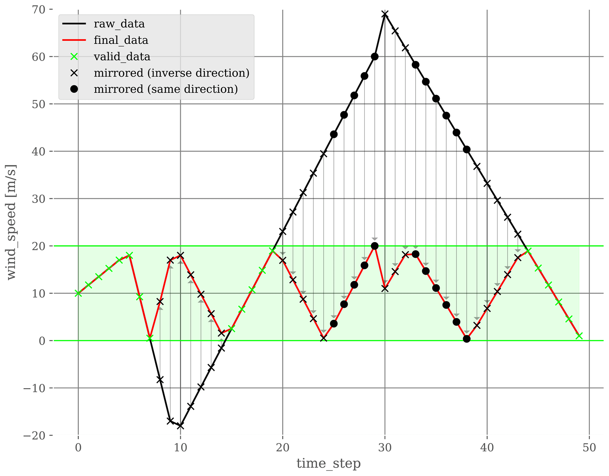
Figure 4 Toy example of the mirrored function used to keep the generated wind speeds inside specific bounds. Raw data are generated thanks to a process described by Algorithm (3). Raw data points inside the wind speed bounds are not modified: the black and red curves overlap. Data points outside the wind speed bounds are recursively mirrored inside the bounds.

The variable ${\mathit{\delta }}_t^X$ defines the level of variation of the wind variable X time series (either the direction or the speed). When equal to 0, the signal is constant. As ${\mathit{\delta }}_t^X$ increases, the absolute value of the increments increases on average. At each time step, ${\mathit{\delta }}_t^X$ is sampled from a uniform distribution defined between ${\mathit{\delta }}_{\text{min}}^X$ and ${\mathit{\delta }}_{\text{max}}^X$. When ${\mathit{\delta }}_{\text{min}}^X$ and ${\mathit{\delta }}_{\text{max}}^X$ are equal, all increments $\mathit{\{}{m}_t{\mathit{\}}}_{t\in \mathit{\{}\mathrm{0},\mathrm{1},\mathrm{\dots },H+L-\mathrm{1}\mathit{\}}}$ are independently sampled from the same distribution: the generated time series is stationary with regard to the increments. When ${\mathit{\delta }}_{\text{min}}^X<{\mathit{\delta }}_{\text{max}}^X$, increments are independently sampled from different distributions: the generated time series is nonstationary with regard to the increments. In Fig. 5 the impact of the ${\mathit{\delta }}_t^K$ variable is shown for the wind direction.

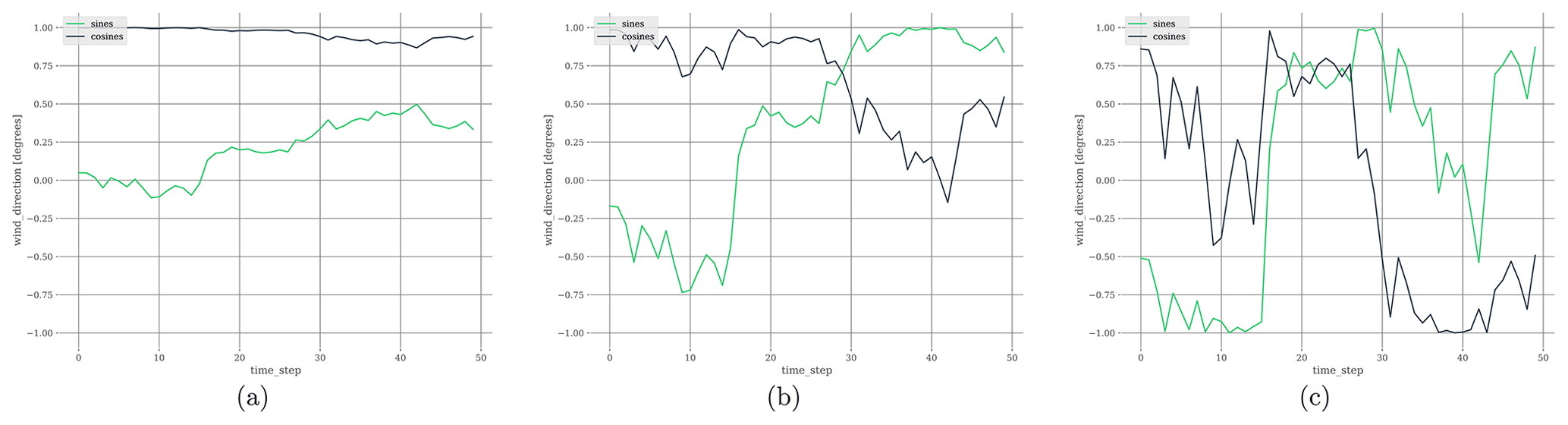
Figure 5 (a) Sine and cosine values for ${\mathit{\delta }}_t^K=\mathrm{1}$. (b) Sine and cosine values for ${\mathit{\delta }}_t^K=\mathrm{4}$. (c) Sine and cosine values for ${\mathit{\delta }}_t^K=\mathrm{9}$. Example of different wind direction signals generated with different ${\mathit{\delta }}_t^K$ values, considering that ${\mathit{\delta }}_t^K={\mathit{\delta }}_{\text{min}}^K={\mathit{\delta }}_{\text{max}}^K$ for all $t\in \mathit{\{}\mathrm{0},\mathrm{1},\mathrm{\dots },\mathrm{49}\mathit{\}}$ and K_init=7°. If ${\mathit{\delta }}_t^K=\mathrm{0}$, all the generated points are equal to K_init. The sine and cosine values are plotted for illustration convenience (it avoids the discontinuity issue of degrees). Note that the behavior shown in this example is the same for the wind speed, but values are in the range [ν_min,ν_max].

4.2 Experimental setting

The function $f_{\text{simulation}}^i(K_t,V_t,\mathit{\{}{\mathit{\alpha }}_{t+\mathrm{1}}^j{\mathit{\}}}_{j\in \mathit{\{}\mathrm{0},\mathrm{1},\mathrm{\dots },N-\mathrm{1}\mathit{\}}})$ computes the local wind speed in front of a turbine i at a time step t given wind data K_t,V_t, and the yaw of each turbine $\mathit{\{}{\mathit{\alpha }}_{t+\mathrm{1}}^j{\mathit{\}}}_{j\in \mathit{\{}\mathrm{0},\mathrm{1},\mathrm{\dots },N-\mathrm{1}\mathit{\}}}$. This function, introduced in Sect. 2.5, is ensured by the low-fidelity, steady-state simulator FLORIS (NREL, 2021). FLORIS is used with a Gauss curl hybrid wake model. The Gaussian velocity model is implemented based on Bastankhah and Porté-Agel (2016) and Niayifar and Porté-Agel (2016). To compute the deflection of the wakes depending on the yaws, the models described by Bastankhah and Porté-Agel (2016) and King et al. (2021) are used. The turbulence model described by Crespo and Hernández (1996) is used. The optional wake modeling options “secondary steering”, “yaw added recovery”, and “transverse velocities”, provided by FLORIS and giving additional features to the $f_{\text{simulation}}^i$ function, are enabled.

A wind farm of 34 International Energy Agency (IEA) identical 15 MW (Gaertner et al., 2020) wind turbines is used. It has cut-in and cut-out speeds of ν_cut-in=3 m s⁻¹ and ν_cut-out=25 m s⁻¹, respectively. Each wind turbine has a rotor diameter of 242.24 m, i.e., a rotor area of 46 087  m². The air density is ρ=1.225 kg m⁻³ and the tunable parameter accounting for the power losses due to misalignment is p=1.88. WFFC strategies are sensitive to the distances between turbines. To make the numerical simulations more robust to the distances between turbines, a diamond shape is used for the layout. With a diamond shape, there is an identical distance between each machine and its surrounding turbines. Using 34 machines creates a sufficiently large wind farm for wake steering to be impactful and is sufficiently small for optimization to converge quickly. A FLORIS illustration of the layout used is given in Fig. 6.

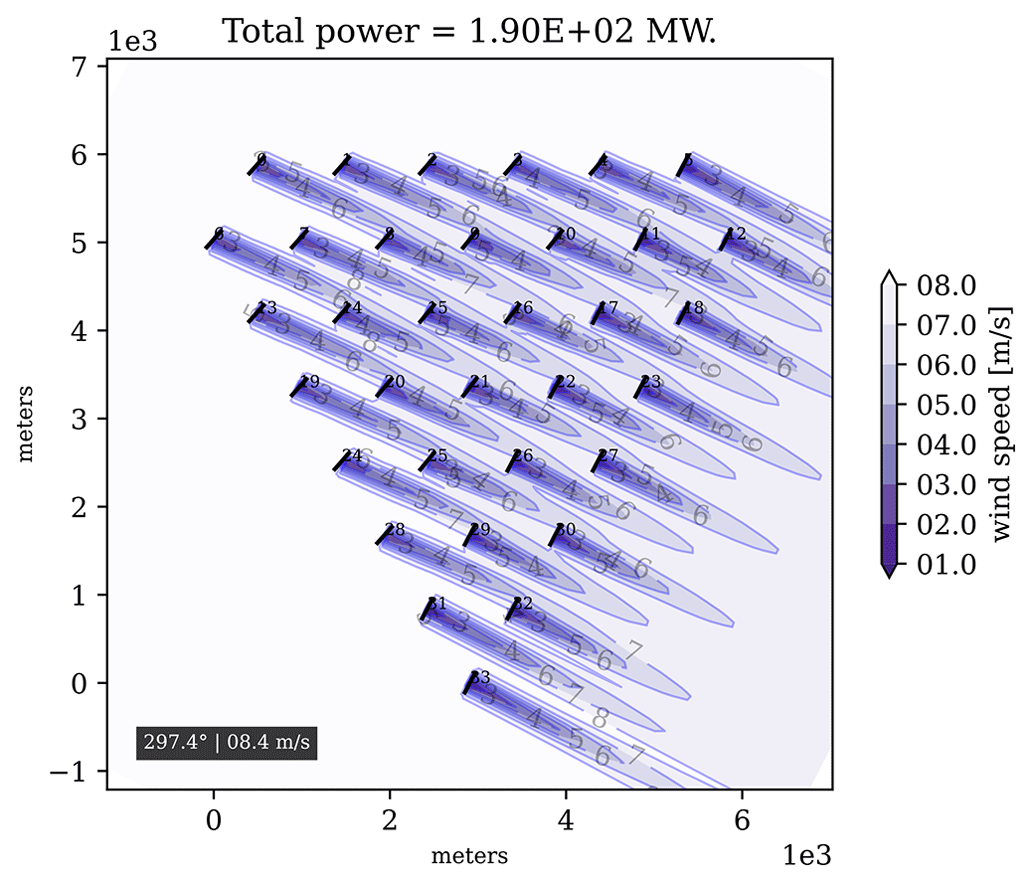
Figure 6 Layout in the form of a diamond shape. The farm comprises 34 identical IEA 15 MW wind turbines. There is an identical space equivalent to the diameter of four turbines between a machine and its adjacent turbines. A distance of four turbine diameters is sufficiently small to create detrimental wake effects for the farm, and therefore the optimization is pertinent and sufficiently large for the design to be realistic. Here the direction is 287.4°, the wind speed is 8.4 m s⁻¹, and yaws are computed with the instantaneous wake steering controller.

The limits for the wind speed are ν_min=4 m s⁻¹ and ν_max=10 m s⁻¹. The interval [4,10] m s⁻¹ approximately corresponds to the ascending part of the power curve, where wake steering is the most beneficial for the farm. For wind speeds of [10,25] m s⁻¹, the power output is constant; if the wind speed is reduced because of wake effects, there will be no power deficit. Because this work conducts a sensitivity analysis of yaw control, the wind speed is kept in the range of [4,10] m s⁻¹.

The horizon size is H=144 and the length of the foresight for the prediction-based controller is L=10. The initial wind values are K_init=270° and V_init=8 m s⁻¹. The discount factor used for the heuristic ℋ_t is γ=0.99. The precision parameter for the GS methods is n_y=120, giving the grid search method good precision.

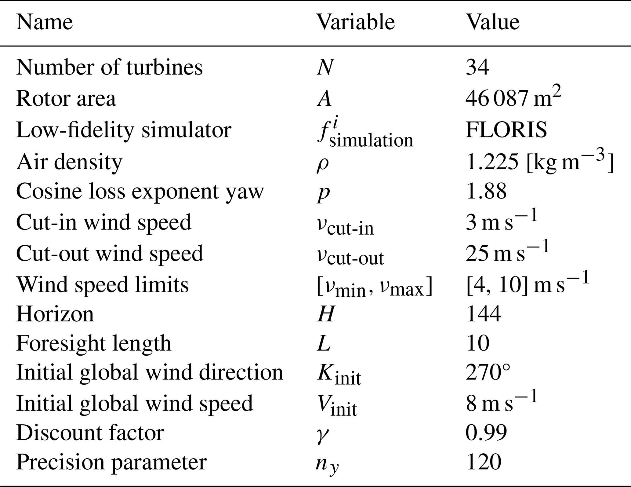
More technical details regarding the simulations and numerical instabilities are given in Appendix B. The time step duration Δt is intentionally undefined, as it will be explained in Sect. 4.3.1. Depending on the time step duration value, different interpretations of the same results will be made. For example, if Δt corresponds to 5 min, then the horizon L=10 means that the prediction-based controller has access to a prediction of the wind of 50 min. In Table 2, a summary of the experimental setting used in this work is given.

Table 2 Detail of the variables and their values used across the simulations. This configuration is shared by all the numerical simulations. The foresight length is equal to 10 only for the prediction-based controller. Otherwise, it is equal to 0. The yaw rotational constraints will vary across the simulations, but α_cut-in and α_cut-out are always equal to u_min and u_max, respectively.

4.3 Results

To empirically demonstrate the importance of optimizing yaw control over a long-term time horizon, numerical simulations are performed with perfect and imperfect (noisy) wind predictions. In the graphs, for each curve, the centerline corresponds to the mean and the colored (shaded) area corresponds to the standard deviation of the results obtained through 11 Monte Carlo trials.

For one episode, the total farm power output of a controller C given by Algorithm (1) is denoted as $P_C={\sum }_{t=\mathrm{0}}^{H-\mathrm{1}}{\sum }_{i=\mathrm{0}}^{N-\mathrm{1}}{P}_t^i$. The metric to benchmark a controller C is the power gain [%] between the total farm power output of C and the total farm power output of the naive controller. The power gain is equal to $\mathrm{100}\cdot \frac{(P_C-P_{\text{naive}})}{P_{\text{naive}}}$.

4.3.1 Perfect predictions

The first set of simulations explores the performance of each controller over increasing variations of wind directions using perfect predictions. Each state comprises perfect information, i.e., ${\mathit{ϵ}}_{K,t}=\mathrm{0}$ and ${\mathit{ϵ}}_{V,t}=\mathrm{0}$ for all $t\in \mathit{\{}\mathrm{0},\mathrm{1},\mathrm{\dots },\mathrm{153}\mathit{\}}$. The performance of each controller presented in Sect. 3 is tested for increasing values of ${\mathit{\delta }}_t^K$.

Numerical simulations are run on 21 different values of ${\mathit{\delta }}_t^K$, with ${\mathit{\delta }}_t^K\in \mathit{\{}\mathrm{0},\mathrm{1},\mathrm{2},\mathrm{\dots },\mathrm{20}\mathit{\}}$. The wind speed is always generated with ${\mathit{\delta }}_t^V=\mathrm{1}$. Because this work explores the impact of wind direction on wake steering, the magnitude of the wind speed fluctuations is kept small. The wind direction and wind speed increments are stationary: ${\mathit{\delta }}_t^K={\mathit{\delta }}_{\text{min}}^K={\mathit{\delta }}_{\text{max}}^K$ and ${\mathit{\delta }}_t^V={\mathit{\delta }}_{\text{min}}^V={\mathit{\delta }}_{\text{max}}^V$ for all $t\in \mathit{\{}\mathrm{0},\mathrm{1},\mathrm{\dots },\mathrm{153}\mathit{\}}$.

The objective here is to study the impact of the wind direction variations on yaw control. The greater the ${\mathit{\delta }}_t^K$ value, the stronger the variations. Because the nacelles have a limited rotational speed, the study of the wind direction fluctuations is crucial for yaw control. The standard deviations of the wind direction time series are related to the ${\mathit{\delta }}_t^K$ parameter in Eq. (32). To better illustrate the wind direction evolution, the time series ΔK defined as

$$\begin{array}{}\text{(33)}& \mathrm{\Delta }K=\mathit{\left\{}\right|f_{\text{yaw}}(K_{t+\mathrm{1}},K_t)|{\mathit{\}}}_{t\in \mathit{\{}\mathrm{0},\mathrm{1},\mathrm{\dots },\mathrm{153}\mathit{\}}}\end{array}$$

is used. Each value of ΔK lies in the range [0,180] [°]. To study the magnitude of the variations, the absolute values are taken. Figure 7 illustrates the influence of some ${\mathit{\delta }}_t^K$ time series on the magnitude of wind direction variations ΔK.

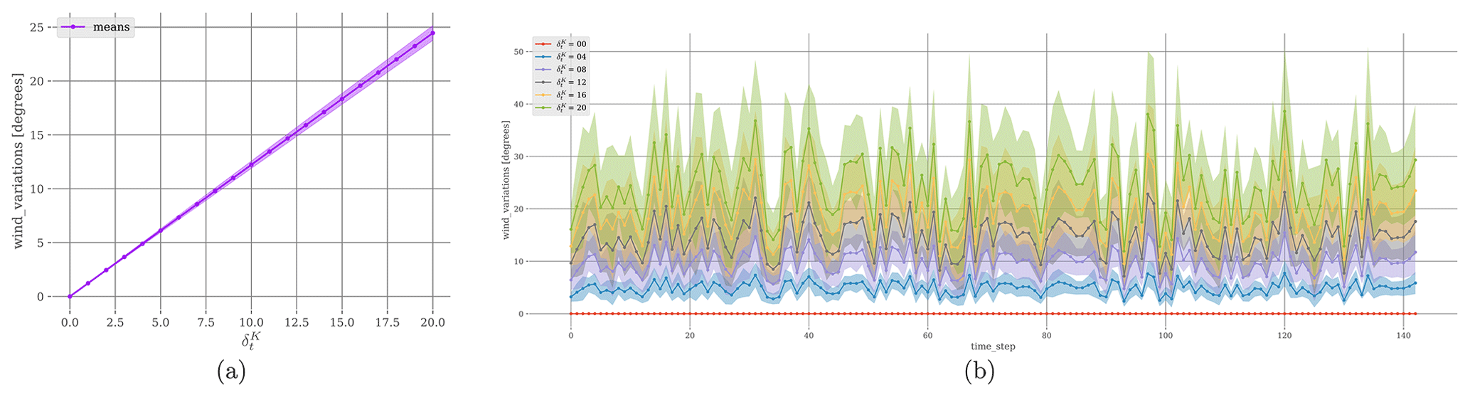
Figure 7 (a) The mean value (and standard deviation) of wind direction variations is given as a function of ${\mathit{\delta }}_t^K$. For example, for ${\mathit{\delta }}_t^K=\mathrm{5}$, the mean absolute variation of the wind direction is around 6.11°. (b) Example of time series ΔK for different values of ${\mathit{\delta }}_t^K\in \mathit{\{}\mathrm{0},\mathrm{4},\mathrm{8},\mathrm{12},\mathrm{16},\mathrm{20}\mathit{\}}$. Again, as the ${\mathit{\delta }}_t^K$ parameter increases, the magnitude of the variations of the wind direction increases.

In Fig. 8, the power gains of each controller compared to a naive controller are plotted. The yaw limits u_min and α_cut-in are equal to −15° (a) or −30° (b). And u_max and α_cut-out are equal to 15° (a) or 30° (b). These yaw constraints offer enough liberty for a wind turbine to rotate between two consecutive time steps and are small enough to limit the induced fatigue. The detailed results are given in Appendix C in Tables C1 and C2.

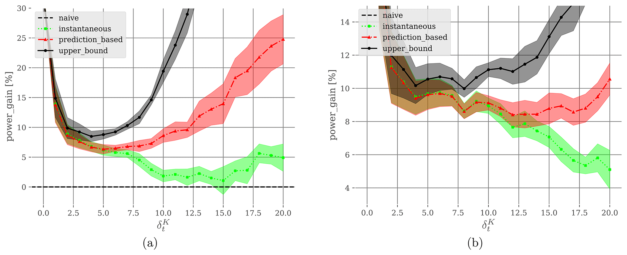
Figure 8 (a) Yaw limits are $u_{\text{min}}={\mathit{\alpha }}_{\text{cut-in}}=-\mathrm{15}$° and $u_{\text{max}}={\mathit{\alpha }}_{\text{cut-out}}=\mathrm{15}$°. At ${\mathit{\delta }}_t^K=\mathrm{6}$, the prediction-based controller increases the power output of a naive approach by 6.23 %. It corresponds to absolute variations of the wind direction of 7.34° as displayed in Fig. 7. (b) Yaw limits are $u_{\text{min}}={\mathit{\alpha }}_{\text{cut-in}}=-\mathrm{30}$° and $u_{\text{max}}={\mathit{\alpha }}_{\text{cut-out}}=\mathrm{30}$°. At ${\mathit{\delta }}_t^K=\mathrm{10}$, the prediction-based controller increases the power output of a naive approach by 8.93 %. It corresponds to absolute variations of the wind direction of 12.23° as displayed in Fig. 7. Considering future wind data in a steady-state yaw control optimization becomes mandatory when ${\mathit{\delta }}_t^k⩾\mathrm{6}$ for yaw constraints $[-\mathrm{15},\mathrm{15}]$° and ${\mathit{\delta }}_t^k⩾\mathrm{10}$ for yaw constraints $[-\mathrm{30},\mathrm{30}]$. From these points, the heuristic ℋ_t provided by the prediction-based controller greatly improves the performance of a classic instantaneous steady-state optimization.

As the variations of the wind direction increase, the performance of each controller diverges from the others. For small variations of the wind direction, both the instantaneous controller and the prediction-based controller give similar results. When the variations of the wind direction become large, the instantaneous controller struggles to maintain good performance. The heuristic of the prediction-based controller manages to find better yaw control strategies. The gap between the performance of the upper bound with the other controllers shows how strong wind direction variations, in relation to the rotational constraints of each machine, impact yaw control.

Based on the results given in Fig. 8, several general statements can be drawn. As previously said, the time step duration is intentionally imprecise. The reason is that different values of Δt will lead to different interpretations. The following statement is true for any values of Δt, with respect to the hypotheses of the transition regime, described in Sect. 2.6.

• For wind turbines that can rotate from −15 to 15° every Δt minutes, if the wind direction changes by more than 7.34° every Δt minutes, it is important to consider future wind data in a steady-state yaw control optimization.

• For wind turbines that can rotate from −30 to 30° every Δt minutes, if the wind direction changes by more than 12.23° every Δt minutes, it is important to consider future wind data in a steady-state yaw control optimization.

4.3.2 Noisy predictions

In the second set of simulations, the robustness to noisy predictions of each controller is tested. The yaw limits are $u_{\text{min}}={\mathit{\alpha }}_{\text{cut-in}}=-\mathrm{15}$° and $u_{\text{max}}={\mathit{\alpha }}_{\text{cut-out}}=\mathrm{15}$°. The $\mathit{\{}{K}_t{\mathit{\}}}_{t\in \mathit{\{}\mathrm{0},\mathrm{1},\mathrm{\dots },\mathrm{153}\mathit{\}}}$ time series are computed with ${\mathit{\delta }}_{\text{min}}^K=\mathrm{0}$ and ${\mathit{\delta }}_{\text{max}}^K=\mathrm{20}$. The time series $\mathit{\{}{V}_t{\mathit{\}}}_{t\in \mathit{\{}\mathrm{0},\mathrm{1},\mathrm{\dots },\mathrm{153}\mathit{\}}}$ are always computed with ${\mathit{\delta }}_t^V={\mathit{\delta }}_{\text{min}}^V={\mathit{\delta }}_{\text{max}}^V=\mathrm{1}$. Because ${\mathit{\delta }}_{\text{min}}^K\ne {\mathit{\delta }}_{\text{max}}^K$, the increments are nonstationary for the wind direction. The corresponding ΔK time series is plotted in Fig. 9.

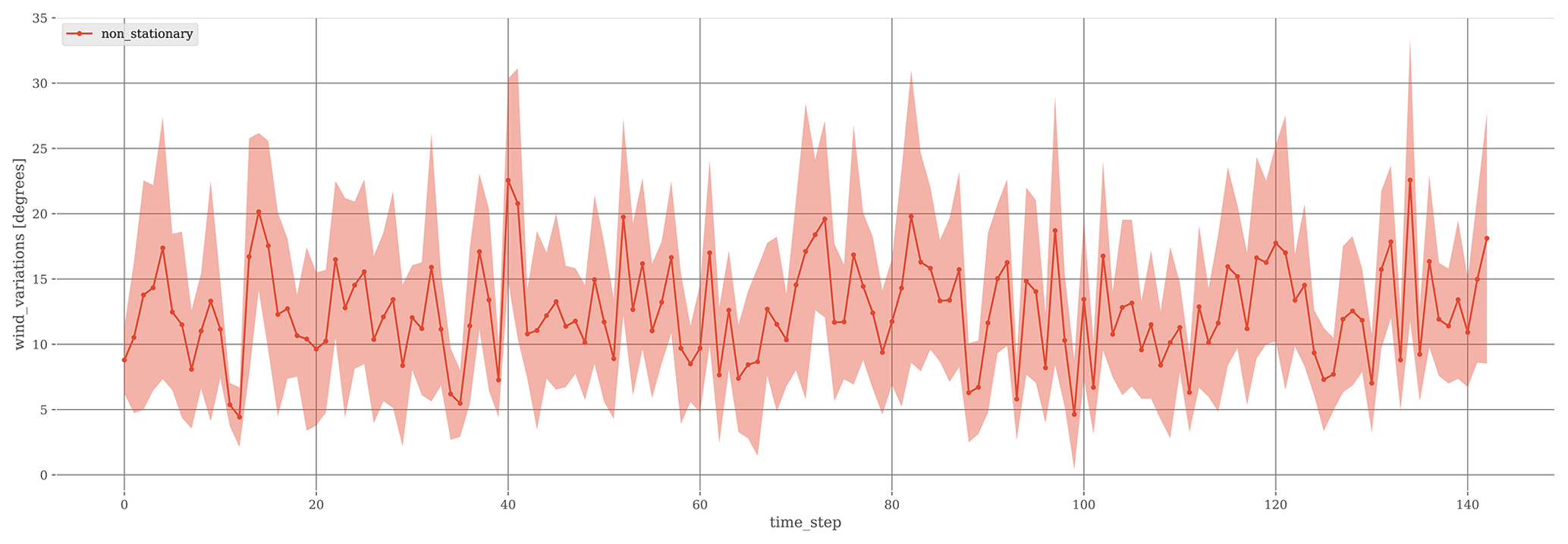
Figure 9 Plot of the time series ΔK for the 11 different seeds. Wind directions are generated with ${\mathit{\delta }}_{\text{min}}^K=\mathrm{0}$ and ${\mathit{\delta }}_{\text{max}}^K=\mathrm{20}$. The mean is 12.53° and the standard deviation is 1.12. Here, the increments vary from one time step to another because they are nonstationary.

In Fig. 10, the noise for the wind direction is increasing, i.e., ${\mathit{ϵ}}_{K,t}\sim U(-z_K,z_K)$ with $z_K\in \mathit{\{}\mathrm{0},\mathrm{1},\mathrm{\dots },\mathrm{15}\mathit{\}}$, for each $t\in \mathit{\{}\mathrm{0},\mathrm{1},\mathrm{\dots },\mathrm{153}\mathit{\}}$. The noise for the wind speed is always sampled from the same distribution, i.e., ${\mathit{ϵ}}_{V,t}\sim U(-\mathrm{1},\mathrm{1})$. In Fig. 10, the noise for the wind speed is increasing, i.e., ${\mathit{ϵ}}_{V,t}\sim u(-z_V,z_V)$ with $z_V\in \mathit{\{}\mathrm{0},\mathrm{1},\mathrm{\dots },\mathrm{7}\mathit{\}}$, for each $t\in \mathit{\{}\mathrm{0},\mathrm{1},\mathrm{\dots },\mathrm{153}\mathit{\}}$. The noise for the wind direction is always sampled from the same distribution, i.e., ${\mathit{ϵ}}_{K,t}\sim U(-\mathrm{1},\mathrm{1})$.

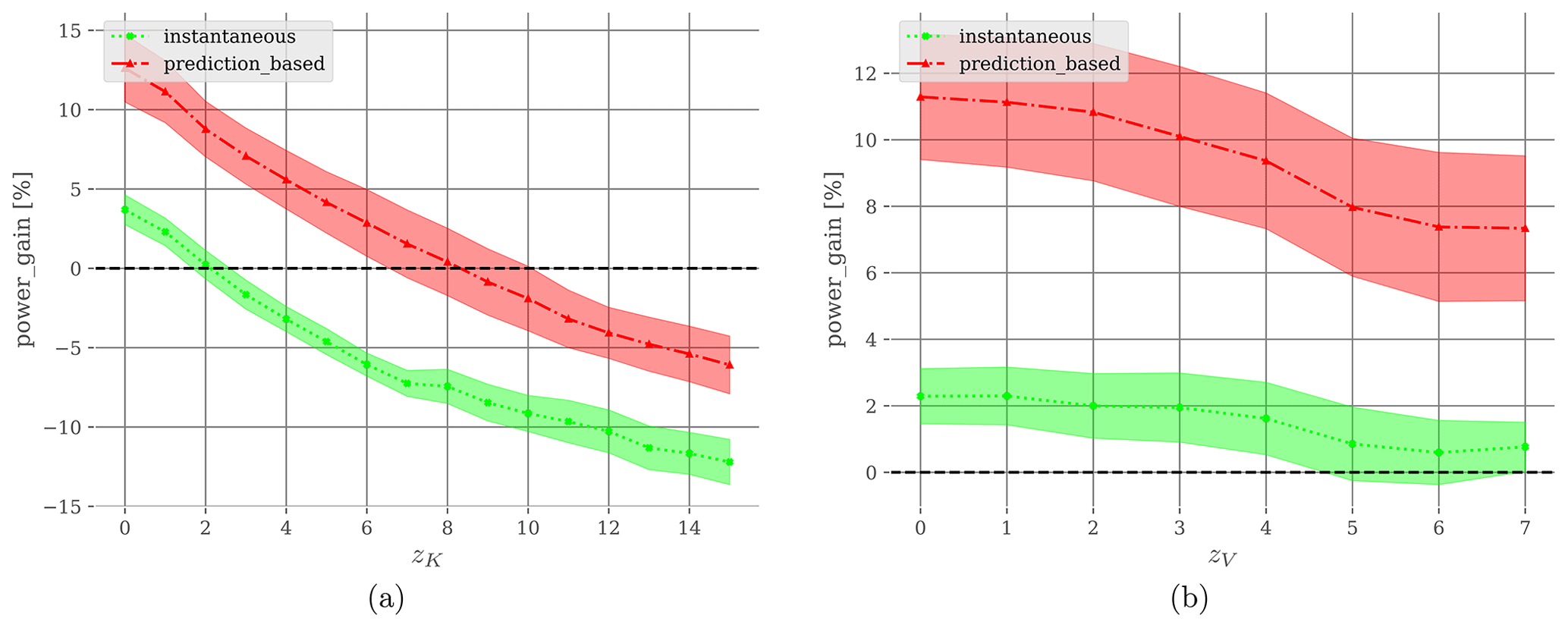
Figure 10 (a) The noises for the wind directions are ${\mathit{ϵ}}_{K,t}\sim U(-z_K,z_K)$ with $z_K\in \mathit{\{}\mathrm{0},\mathrm{1},\mathrm{\dots },\mathrm{15}\mathit{\}}$ for each $t\in \mathit{\{}\mathrm{0},\mathrm{1},\mathrm{\dots },\mathrm{153}\mathit{\}}$. The noise for the wind speeds is always sampled from a uniform distribution $U(-\mathrm{1},\mathrm{1})$. (b) The noises for the wind speeds are ${\mathit{ϵ}}_{V,t}\sim U(-z_V,z_V)$ with $z_V\in \mathit{\{}\mathrm{0},\mathrm{1},\mathrm{\dots },\mathrm{7}\mathit{\}}$ for each $t\in \mathit{\{}\mathrm{0},\mathrm{1},\mathrm{\dots },\mathrm{153}\mathit{\}}$. The noise for the wind directions is always sampled from a uniform distribution $U(-\mathrm{1},\mathrm{1})$.

Only the noise applied to the wind directions strongly impacts the different policies. The prediction-based controller results in a poorer performance than a naive controller from a noise of 8°. The wind speed noise insignificantly affects the performance of the algorithms. This corroborates the fact that yaw control mainly depends on the wind directions. Because the prediction-based controller uses more wind data points, it is more robust than the instantaneous controller.

5 Conclusions

As WFFC is becoming more important to increase the energy production of wind farms, this work studies wake steering as a steady-state optimization problem over time. The yaw control problem is formalized as successive multiple steady-state optimization problems interconnected by the rotational constraints of the turbines and the evolution of the wind. Because the function computing the power outputs is steady-state, only the dynamics of a homogeneous global wind and the rotational constraints of the machines are captured. Low-fidelity, steady-state simulators are used because they are not time-consuming and they are suitable for optimization. But future works should perform the same studies with continuous and higher-fidelity simulators such as HAWC2Farm (Liew et al., 2023), better capturing the dynamics of the wake effects from one time step to another. This becomes especially important when the variations of the wind direction become important.

Traditionally, yaw control is optimized in a steady-state manner. Yaw settings are computed so that they maximize the instantaneous power output of the farm. To optimize wake steering over a long-term time horizon, an MPC method is usually used. Such an approach increases the complexity of the optimization problem, making it harder to solve. To overcome such complexity, a reformulation of the steady-state optimization problem is proposed in this work to consider future wind data. The traditional objective function is augmented by a new heuristic estimating the future expected theoretical power outputs of the farm, weighted by how far the turbines will be from the wind if they are controlled by a naive approach. The new prediction-based controller proposed in this paper has the same number of decision variables as an instantaneous optimization.

Lastly, this work conducts a sensitivity analysis of yaw control and the variations of the wind direction. It demonstrates the importance of optimizing yaw control over future wind data when the variations of the wind directions become large. For strong wind variations, the new prediction-based controller greatly improves the performance without increasing complexity. This work shows, for example, that if deploying wind turbines that can rotate from −15 to 15° every Δt minutes, and if the wind direction changes by more than 7.34° every Δt minutes, it is important to consider future wind data in a steady-state yaw control optimization. Experiments empirically show the effectiveness of the simplifications proposed in this work in a specific experimental setting, but future research could better justify and quantify their impact on the original prediction-based decision problem.

This study is conducted on synthetic wind data so future works should explore the same question of dependence between the wind variations and yaw control over real wind data. Because the hypotheses regarding the transition regime may be far from reality, the proposed heuristic could be combined with low-pass filters and hysteresis mechanisms for more realistic implementations. Future works should incorporate the fatigue in the optimization process, as WFFC can have a major impact on the lifetime of each turbine. For example, the objective function of the prediction-based controller could be augmented by a heuristic taking into account the magnitude of the yaw actuations. However, the results provided by this work also suggest that with wake steering strategies more robust to wind direction variations, it would be possible to reach the same level of performance with fewer yaw actuations.

Appendix A: Gauss–Seidel method

Algorithm A1 GS method.

Input: s_t input state

$c{x}_t^i,c{y}_t^i=(c{x}^i,c{y}^i)\cdot \left(\begin{array}{cc}\cos (\mathrm{270}-K_t^{\prime })& -\sin (\mathrm{270}-K_t^{\prime })\\ \sin (\mathrm{270}-K_t^{\prime })& \cos (\mathrm{270}-K_t^{\prime })\end{array}\right)$

▹ rotate turbines

$R=\mathit{\{}{i}_{\mathrm{0}},i_{\mathrm{1}},\mathrm{\dots },i_{N-\mathrm{1}}|c{x}_t^{i_{\mathrm{0}}}⩽c{x}_t^{i_{\mathrm{1}}}⩽\mathrm{\dots }⩽c{x}_t^{i_{N-\mathrm{1}}}\mathit{\}}$

▹ order turbines

$(u_{t,\mathrm{0}}^{i_{\mathrm{0}}},u_{t,\mathrm{0}}^{i_{\mathrm{1}}},\mathrm{\dots },u_{t,\mathrm{0}}^{i_{N-\mathrm{1}}})={\mathit{\pi }}_{\text{naive}}\left(s_t\right)$

▹ initialize yaw settings

for i∈R do

$S=\mathit{\{}{u}_{\text{min}}+l\cdot \frac{u_{\text{max}}-u_{\text{min}}}{n_y-\mathrm{1}}\mathit{\}},\forall l\in \mathit{\{}\mathrm{0},\mathrm{1},\mathrm{\dots },n_y-\mathrm{1}\mathit{\}}$

▹ discretized solution space

$U=(u_{t,\mathrm{1}}^{i_{\mathrm{0}}},u_{t,\mathrm{1}}^{i_{\mathrm{1}}},\mathrm{\dots },u^i,\mathrm{\dots },u_{t,\mathrm{0}}^{i_{N-\mathrm{2}}},u_{t,\mathrm{0}}^{i_{N-\mathrm{1}}})$

▹ fix all other settings

$u_{t,\mathrm{1}}^i\in \underset{u^i\in S}{\arg max}{f}_{\text{obj}}(s_t,U)$

▹ grid search optimization

end for

Output: $(u_{t,\mathrm{1}}^{i_{\mathrm{0}}},u_{t,\mathrm{1}}^{i_{\mathrm{1}}},\mathrm{\dots },u_{t,\mathrm{1}}^{i_{N-\mathrm{1}}})$ yaw settings

The GS method iterates over each turbine in the direction of the wind, one by one, from upstream turbines to downstream ones. The turbines' default coordinates $\mathit{\{}c{x}^i,c{y}^i{\mathit{\}}}_{i\in \mathit{\{}\mathrm{0},\mathrm{1},\mathrm{\dots },N-\mathrm{1}\mathit{\}}}$ [m] are rotated such that the wind is coming from the west. The initial yaw settings are computed with a naive controller. By doing so, the initial solution is already a good enough solution that keeps turbines as aligned with the wind as possible. At each iteration, it solves the optimization problem by varying the yaw setting of the current turbine, considering all the others fixed. To solve each optimization problem on one variable, a grid search approach over a discretized solution space S is used. Once solved, the setting for turbine k is fixed and optimization is conducted again on turbine k+1. Such an approach gives good results because it exploits the sequential nature of the low-fidelity simulation.

Appendix B: Numerical instabilities

First, some modifications have been made to FLORIS in order to shut down turbines misaligned too much with the wind during a simulation. At a time step t, for a given turbine i, all the possible yaw settings can give a similar power output. In such cases, the best yaw setting is the one staying the closest to the wind direction in order to prevent future misalignment. To incorporate such behavior in the optimization process and to make the controllers robust to numerical instabilities, the following steps are taken.

• Round out the power output computed by the simulator.

• Take the yaw setting $u_t^i$ maximizing the objective function.

• Find all the yaw settings giving a performance close to the maximum.

• Among these selected settings, keep the one closest to the setting corresponding to the naive controller.

To compute the solutions of the upper-bound controller described in Sect. 3.3, a trick is used. Relaxing the rotational constraints of the turbines, i.e., making u_min and u_max equal to −180 and 180°, respectively, increases the solution space. With the same precision parameter n_y, it reduces the precision of the grid search method. To keep the solution space between u_min and u_max, and therefore not to alter the precision of the grid search method, the evolution of the system described in Algorithm (1) is slightly modified. At the beginning of each time step, every turbine is realigned with the wind direction. Such a trick does not alter the solutions given by the upper-bound controller because good yaw settings are the ones keeping turbines close to the wind direction.

Appendix C: Detailed results

Table C1 Detailed results of the simulations conducted on perfect predictions in Sect. 4.3.1. Yaw limits are $u_{\text{min}}={\mathit{\alpha }}_{\text{cut-in}}=-\mathrm{15}$° and $u_{\text{max}}={\mathit{\alpha }}_{\text{cut-out}}=\mathrm{15}$°. For each ${\mathit{\delta }}_t^K$ the total power output of the farm in 10⁴ MW is given for each controller.

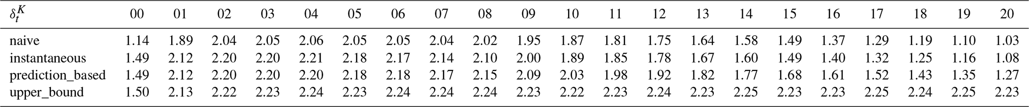
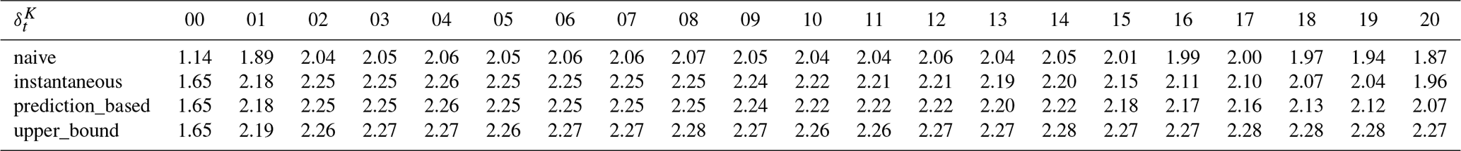
Table C2 Detailed results of the simulations conducted on perfect predictions in Sect. 4.3.1. Yaw limits are $u_{\text{min}}={\mathit{\alpha }}_{\text{cut-in}}=-\mathrm{30}$° and $u_{\text{max}}={\mathit{\alpha }}_{\text{cut-out}}=\mathrm{30}$°. For each ${\mathit{\delta }}_t^K$ the total power output of the farm in 10⁴ MW is given for each controller.

Appendix D: Nomenclature

N	Number of wind turbines
Δt	Time step duration
H	Horizon length
Kt	Wind direction
Vt	Wind speed
$K_t^{\prime }$	Observed wind direction
$V_t^{\prime }$	Observed wind speed
${\mathit{\nu }}_t^i$	Local wind speed
${\mathit{\beta }}_t^i$	Absolute orientation
${\mathit{\alpha }}_t^i$	Yaw angle
fyaw	Yaw angle computation function
$u_t^i$	Yaw setting
fcontrol	Absolute orientation update function
Φ	Theoretical power output function
fpower	Power output function
st	Controller state
ϵK,t	Wind direction noise
ϵV,t	Wind speed noise
fsimulation	Local velocities computation function
$P_t^i$	Turbine power output
π	Control policy
ut	All turbine yaw settings
fobj	Controller objective function

Appendix E: Acronyms

FLORIS	FLOw Redirection and Induction in Steady State
GS	Gauss–Seidel
IEA	International Energy Agency
LESs	large-eddy simulations
LUT	lookup table
ML	machine learning
MPC	model predictive control
MW	megawatts
RL	reinforcement learning
WFFC	wind farm flow control