Active trailing edge flap system fault detection via machine learning

Active trailing edge flap (AFlap) systems have shown promising results in reducing wind turbine (WT) loads. The design of WTs relying on AFlap load reduction requires implementing systems to detect, monitor, and quantify any potential fault or performance degradation of the flap system to avoid jeopardizing the wind turbine's safety and performance. Currently, flap fault detection or monitoring systems are yet to be developed. This paper presents two approaches based on machine learning to diagnose the health state of an AFlap system. Both approaches rely only on the sensors commonly available on commercial WTs, avoiding the need and the cost of additional measurement systems. The first approach combines manual feature engineering with a random forest classifier. The second approach relies on random convolutional kernels to create the feature vectors. The study shows that the first method is reliable in classifying all the investigated combinations of AFlap health states in the case of asymmetrical flap faults not only when the WT operates in normal power production but also before startup. Instead, the second method can identify some of the AFlap health states for both asymmetrical and symmetrical faults when the WT is in normal power production. These results contribute to developing the systems for detecting and monitoring active flap faults, which are paramount for the safe and reliable integration of active flap technology in future wind turbine design.

1 Introduction

The pursuit of lower levelized cost of energy has driven a steady increase in the size of utility-scale wind turbines (WTs) over the past years, with a consequent increase in the load carried by the WT components. Among the new technologies studied to mitigate this load increase, actively controlled flaps located at the blade trailing edge (AFlap) have shown promising results in reducing fatigue and ultimate loads and increasing annual energy production, see Barlas et al. (2016) and Pettas et al. (2016). Despite the potential benefits of AFlaps, this technology has yet to reach a sufficient level of maturity for its implementation in commercial WTs. To the authors' knowledge, only Siemens Gamesa Renewable Energy (SGRE) has publicly shared data of an AFlap system implemented on two different multi-megawatt WTs: a 4.0 MW WT prototype and a 4.3 MW WT prototype, both installed in Høvsøre (Denmark); see Gomez Gonzalez et al. (2022).

Every time a new component is included in a wind turbine's design, the safe and reliable continuous wind turbine operation must be ensured for the whole turbine's lifetime. To fulfill this requirement, additional components, systems, and controller strategies are needed to identify, quantify, and resolve any potential issue deriving from the fault of the new component without compromising the WT safety. Once the active flap reaches an adequate level of maturity, the wind turbine design will rely on the load reduction provided by the active flap. Therefore, any potential fault or performance degradation of the flap system may jeopardize the safety and performance of the wind turbine if not adequately managed. Therefore, a system will be needed to identify, monitor, and manage active flap faults or degradation. Until now, the fault diagnosis and condition monitoring of AFlap systems has not been investigated in detail, and to our knowledge, no literature is available on this topic. Nevertheless, we can foresee different approaches for AFlap fault diagnosis and monitoring, following the standard methodologies currently applied in the wind energy sector, for which Hossain et al. (2018) and Gao and Liu (2021) provide comprehensive and updated overviews.

As a first approach, monitoring and diagnosis can rely on dedicated sensors located in specific mechanical elements, like a vibration sensor in a gearbox (Zappalá et al., 2014). For the AFlap system, position or pressure sensors could be located on the flap surfaces or in their proximity to quantify the AFlap deflection or the AFlap impact on the blade aerodynamics. Due to the expected large blade area covered by the flaps, this monitoring approach will require several sensors distributed along the outer third of the blade length. This system will likely be complex, expensive to deploy and maintain, sensitive to lighting, and affected by the reliability of the sensor operating in the harsh environment of a wind turbine rotating blade.

The second approach is the model-based method that mainly relies on the analyses of the residual signals, signals defined as the difference between the real system outputs and the output from a model of the system created by using, for example, Kalman filter, observers, or model-based machine learning techniques. On WTs, the model-based methods have been applied, for example, in the condition monitoring of main bearings (de Azevedo et al., 2016), sensors and actuators (Cho et al., 2018), and generators (Gálvez-Carrillo and Kinnaert, 2011). As a drawback, the model-based methods require a reasonably good model to guarantee the detection of faults. The model generation could be challenging for AFlap fault detection mainly due to the high nonlinearity of the WT blade dynamic, the high uncertainty on the wind field interacting with the WT rotor, and the limited number of sensor measurements available on a commercial WT. Improved wind field estimations (e.g., from nacelle Lidar) or additional load or pressure sensors on the blade can facilitate the model generations and improve their accuracy at the price of an increased system complexity and cost.

Finally, data-driven methods allow fault detection without needing a detailed system model but by several types of data and signal analyses. These analyses range from the simple detection of changes in mean values, variances, or trends to the more advanced machine learning (ML) methodologies (Badihi et al., 2022). In particular, the study and application of ML methodologies to fault diagnosis and condition monitoring has increased exponentially in recent years thanks to the technological and computational advances that have allowed us to quickly and efficiently analyze the large amount of data needed for the training of the ML models (García Márquez and Peinado Gonzalo, 2022). Overviews of the machine learning methods for wind turbine condition monitoring are provided by Stetco et al. (2019) and Malekloo et al. (2022). ML techniques can be applied for the AFlap fault detection if a sufficient amount of relevant data can be provided for the model training. Currently, the amount of AFlap field data is limited – even more for AFlap faults. Nevertheless, aeroelastic simulations have been commonly used for WT design. Therefore, it is reasonable to assume that a sufficiently accurate aeroelastic model of a WT equipped with AFlap can be used to train an ML model for the AFlap fault detection. To test this assumption, in this paper we study if data-driven methods based on ML trained with aeroelastic simulation can adequately classify the AFlap fault states.

1.1 Detecting AFlap health state

The detection of the health state of the AFlap is a challenging task. Figure 1a shows the mean blade root moment when the flap is deactivated (AF_Off) or is active without performance degradation (AF_On) as a function of the wind speed. As expected, AFlaps have a relevant impact on the WT blade aerodynamic, visible in the two distinct lines of the mean moment binned as a function of the wind speed. However, the broad range of environmental conditions where the WT operates causes the moment to vary within a wide range of values, a range shown in the plot by the colored areas. These areas overlap significantly, making it difficult for a detection system to identify the actual AFlap health state. Figure 1b shows the time series of the blade root bending moment for the AFlap active and AFlap not active with the same 10 m s⁻¹ turbulent wind. The two lines have a similar highly oscillating behavior with just a small shift due to the increased lift generated by the flap activation.

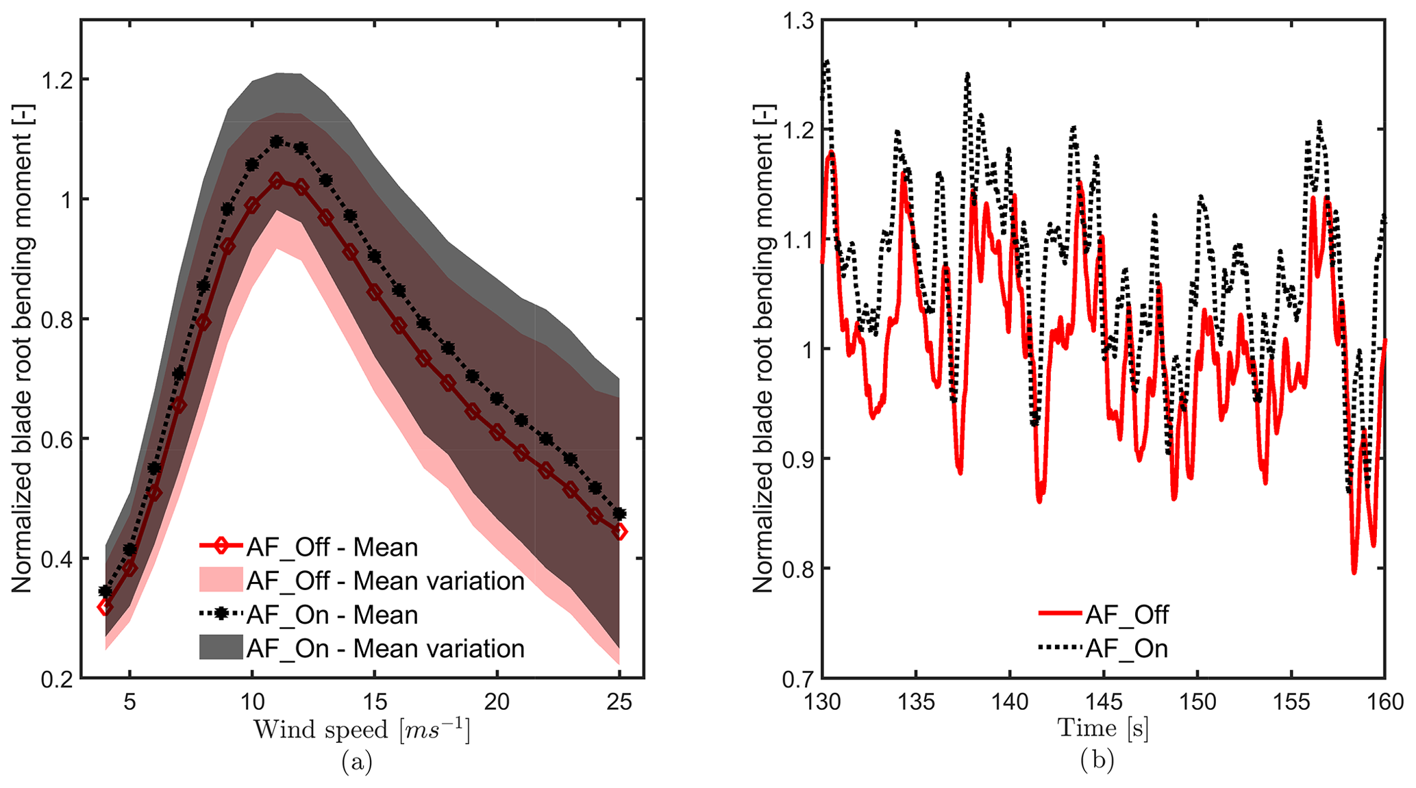
Figure 1 (a) Mean value of the normalized blade root bending moment when the AFlap is deactivated (AF_Off) and activated without degradation (AF_On), binned as a function of the wind speed. (b) Example of time series of the normalized blade root bending moment when the AFlap is deactivated (AF_Off) and activated without degradation (AF_On) for a 10 m s⁻¹ turbulent wind.

Furthermore, several faults of the AFlap system can occur in the WT lifetime, which behavior and severity depend on the layout and scope of the AFlap system itself. Wear and tear can slowly degrade the performance of part of the AFlap system; ice or lightning can instead compromise the whole system's functionality. As it is impossible to evaluate all the different combinations of faults, we selected a set of representative conditions we believe can cover a wide range of flap faults. The selected cases cover partial and complete performance degradation happening only on one blade or on all three blades simultaneously. We focus on identifying the AFlap health state in static flap actuation to keep the approach as general as possible. This approach keeps the detection system independent from any specific AFlap controller strategy, AFlap system design, or fault dynamics. The idea is to integrate this kind of detection system in an AFlap status check routine running for several minutes in which the performance of the stationary flap is verified.

1.2 Research contribution

This paper investigates whether a simple ML algorithm can assess the health of an active trailing edge flap system from the data provided by the sensors commonly available on a commercial WT. The aim is to develop a system that does not require any additional sensor to be installed on the WTs, making it easy to implement without relevant additional costs for installation or maintenance. This task can be seen as a multivariate time-series classification problem where the ML algorithm aims to estimate if the AFlap is properly operating or is affected by performance degradation. We follow two different approaches for computing the features from the sensors' time-series data. In the first approach, we select the features based on our knowledge of the impact of AFlaps on the different WTs signals. In the second approach, we use a brute force approach to explore possible unknown correlations between AFlaps' states and variations in the WTs signals. This approach relies on thousands of randomly generated convolutional kernels that automatically compute features from all the available signals without requiring pre-knowledge of AFlaps. We select the simple but robust random forest classifier for both feature calculation approaches. Aeroelastic simulations are used to train and test the ML models. We use the aeroelastic model developed by Gamberini et al. (2022) of the 4.3 MW WT prototype owned by SGRE, where a 20 m AFlap was installed and tested on one blade of the 120 m diameter rotor.

Section 2 describes the aeroelastic model, the environmental conditions, and the flap health states used in the aeroelastic simulations. In Sect. 3, we describe the ML methodologies used in the study and the two approaches used for AFlap health detection. In Sects. 4 and 5, we show the obtained results that we discuss in Sect. 6.

2 Simulated experiments

The training of the ML models is based on a pool of aeroelastic simulations reproducing the WT aeroelastic response for the combination of wind turbine operative conditions and flap health states of interest.

2.1 Aeroelastic simulations

A set of aeroelastic simulations is computed for every combination of wind turbine operative conditions and flap health state of interest. We computed all sets with the same WT aeroelastic model.

We accounted for the influence of the variability in the environmental conditions on the wind turbine's aeroelastic response by defining the main environmental conditions as random variables of pre-imposed statistical properties.

2.1.1 Environmental conditions

Table 1 shows the environmental conditions modeled as random variables and their parameters, which are the following.

• Mean wind speed. This follows a Weibull distribution with the annual average wind speed set to 10 m s⁻¹ and the shape parameter to 2. It is equivalent to IEC wind class 1.

• Wind turbulence intensity. This follows the normal turbulence model described in the IEC 61400-1:2019 (IEC, 2019) for turbulence class A where Iref is set to 0.16 with a lognormal distribution. It is defined as

  $$\begin{array}{}\text{(1)}& {\displaystyle }& {\displaystyle }E\left[{\mathit{\sigma }}_U|U\right]=I_{\mathrm{ref}}(\mathrm{0.75}U+\mathrm{3.8}),\text{(2)}& {\displaystyle }& {\displaystyle }\mathrm{Var}\left[{\mathit{\sigma }}_U|U\right]={\left(\mathrm{1.4}{I}_{\mathrm{ref}}\right)}^{\mathrm{2}}.\end{array}$$

• Wind shear exponent. The vertical wind profile is modeled with a power law with exponent α. As proposed by Dimitrov et al. (2015), the wind shear exponent is normally distributed and conditionally dependent on the mean wind speed U as follows:

  $$\begin{array}{}\text{(3)}& {\displaystyle }& {\displaystyle }E\left[\mathit{\alpha }\right|U]=\mathrm{0.088}(\ln \left(U\right)-\mathrm{1}),\text{(4)}& {\displaystyle }& {\displaystyle }\mathrm{Var}\left[\mathit{\alpha }\right|U]={\left({\displaystyle \frac{\mathrm{1}}{U}}\right)}^{\mathrm{2}},\end{array}$$

  where α values are constrained within realistic limits.

• Horizontal inflow angle. Ψ follows a normal distribution, is truncated within realistic limits, and is conditionally dependent on the mean wind speed U as proposed by Duthé et al. (2021):

  $$\begin{array}{}\text{(5)}& {\displaystyle }& {\displaystyle }E\left[\mathrm{\Psi }\right|U]=\ln (U)-\mathrm{3},\text{(6)}& {\displaystyle }& {\displaystyle }\mathrm{Var}\left[\mathrm{\Psi }\right|U]={\left({\displaystyle \frac{\mathrm{15}}{U}}\right)}^{\mathrm{2}}.\end{array}$$

• Vertical inflow angle and air density. Normally distributed, they are truncated within reasonable limits, with prescribed values of mean and standard deviation.

One example set of environmental conditions is sampled for the pre-startup cases, shown in Fig. 2, and the normal power production cases, shown in Fig. 3.

Table 1 Parameters of the environmental conditions modeled as random variables.

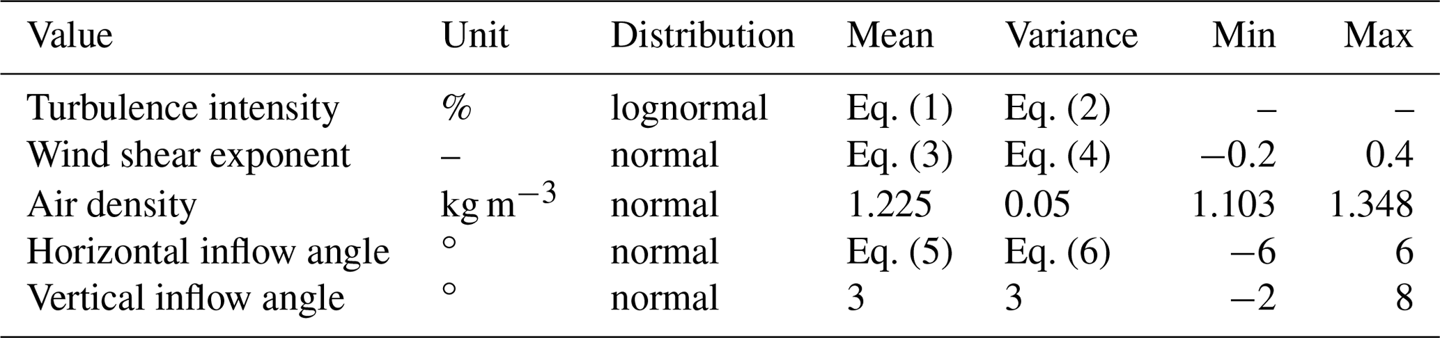
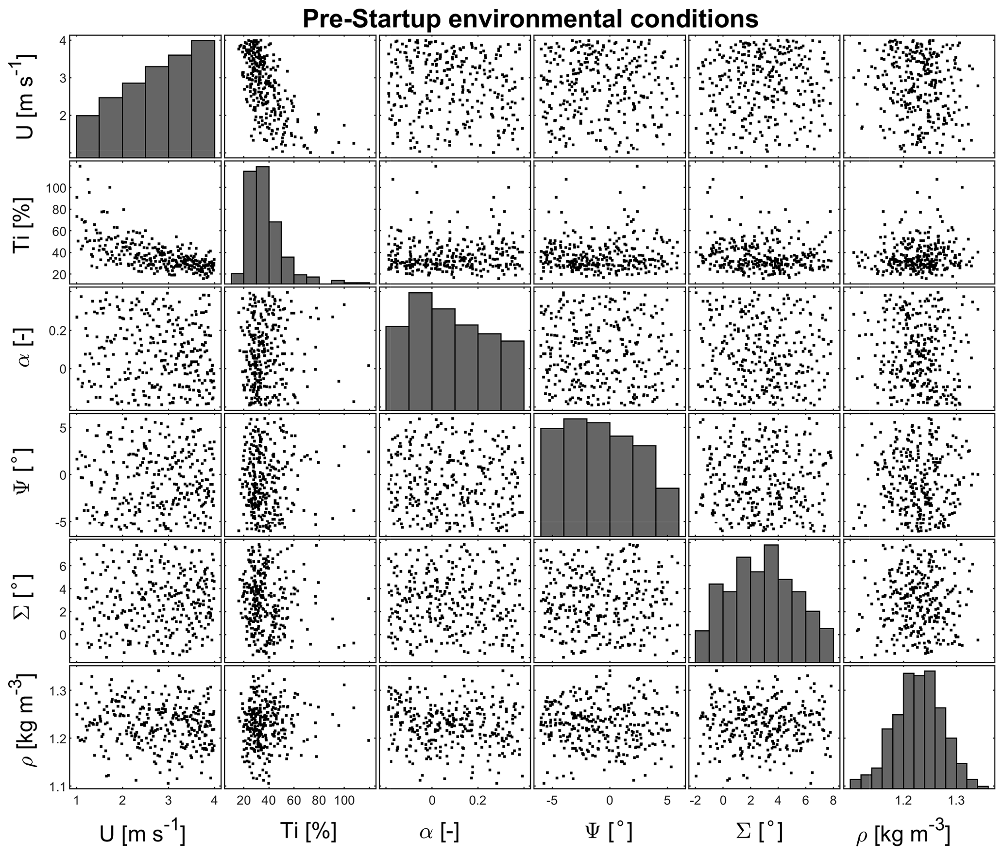
Figure 2 Example of environmental conditions for pre-startup simulations: mean wind speed U, wind turbulence intensity TI, wind shear exponent α, horizontal inflow angle Ψ, vertical inflow angle Σ, and air density ρ.

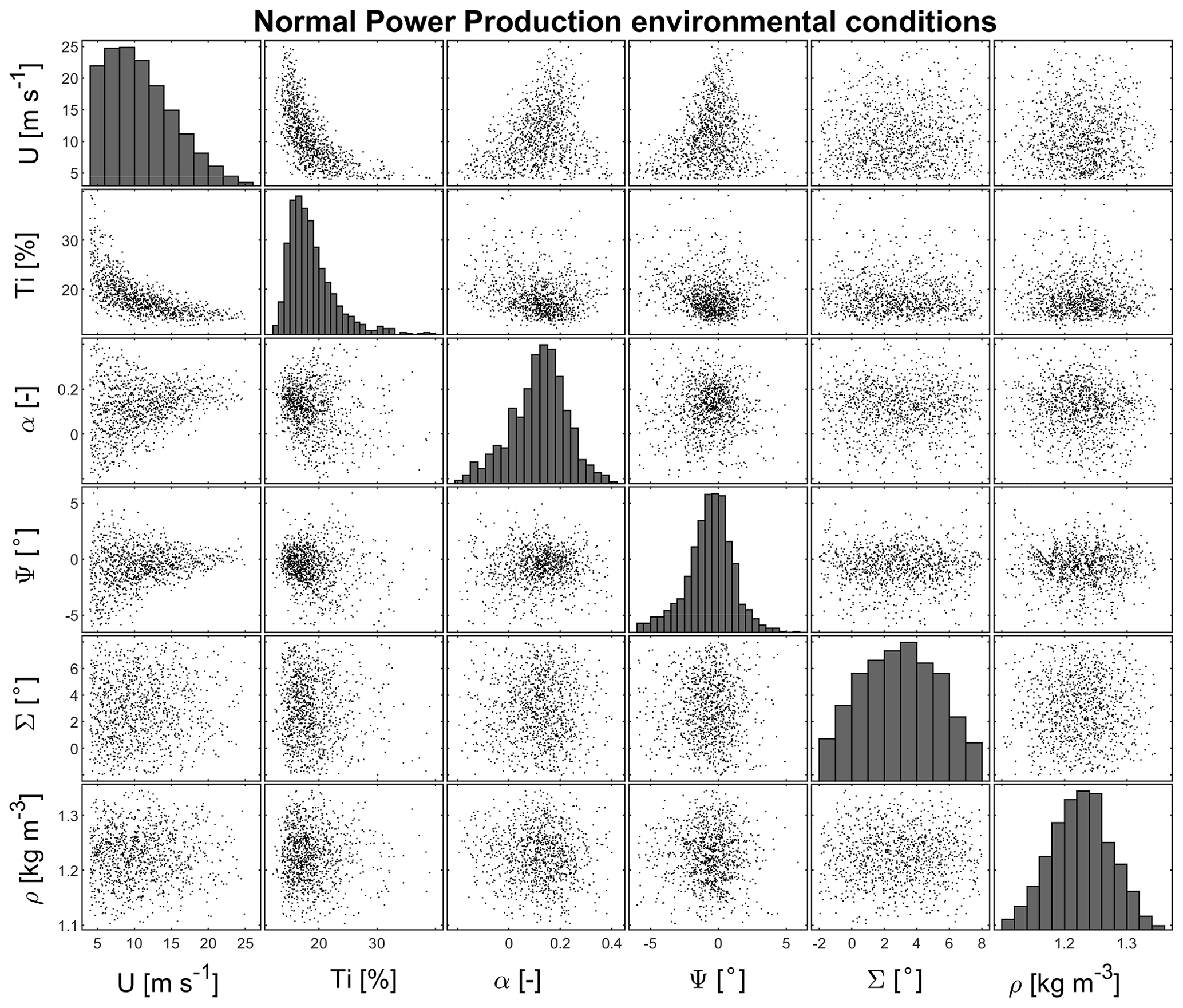
Figure 3 Example of environmental conditions for normal power production simulations: mean wind speed U, wind turbulence intensity TI, wind shear exponent α, horizontal inflow angle Ψ, vertical inflow angle Σ, and air density ρ.

2.1.2 Aeroelastic model and simulation setup

BHawC is the aeroelastic engineering tool developed internally by SGRE. It is based on the blade element momentum (Fisker Skjoldan, 2011) and models the AFlap's aerodynamic and actuator system with a dedicated flap module.

SGRE provided the BHawC model of the prototype wind turbine (pWT) used for the aeroelastic simulations. It includes the pWT's structural and aerodynamic models and its controller. The AFlap model is also tuned to match the lift increase in the blade region covered by the flap when activated. In Gamberini et al. (2022), one of the authors showed that this model estimates the pWT operational parameters and blade loads with reasonable accuracy, and the AFlap activation increases up to +8 % the mean flapwise bending moment at the blade root. All simulations have the same pWT BHawC model, with only changes in the environmental conditions and the AFlap health state. The simulations are performed with turbulence wind and are 10 min long with a 0.01 s time step length.

Two operative conditions are simulated: normal power production (NPP) and pre-startup (PS). In the latter cases, the wind turbine is in idling condition with the controller optimizing the blade pitch angle to bring the rotor speed and generator torque to the startup conditions.

For every operative condition, asymmetrical and symmetrical AFlap fault cases are simulated. In the symmetrical flap fault case (3B), the flaps on the three blades have all the same state and performance. This means the three flaps are modeled with the same aerodynamic polars and control signal. In the asymmetrical case (1B), the AFlap is active only on one blade. Even if this is not an expected configuration for future wind turbines, this setup mirrors the pWT setup facilitating a future testing with the pWT measurements data. Furthermore, the rotor imbalance due to the flap activated on only one blade is still a good approximation of the imbalance due to a flap on one blade being at a different state or performance than the flaps on the other two blades.

For every case, we simulated seven different AFlap health states.

• Flap off (AF_Off). AFlap is not active and is simulated with baseline aerodynamic polar and flap control off.

• Flap on (AF_On). AFlap is active and is simulated with active flap aerodynamic polar and flap control on.

• Flap off with fault (AF_Off_Fault). AFlap is active even if the control commands it to be not active. This state can simulate the case when ice formed on the blades prevents the flap from closing. It is simulated with active flap aerodynamic polar and flap control off.

• Flap on with fault (AF_On_Fault). AFlap is not active even if the control commands it to be active. This state can be caused by ice preventing the flap from opening or the flap actuator not working. It is simulated with baseline aerodynamic polar and flap control on.

• Flap on with degradation. AFlap is active but with degraded performance. Reduced flap deflections due to reduced flap actuator operation, material aging, or extremely low temperature can be associated with these cases. We simulated AFlap performance reduced to 25 % (AF_On_25pc), 50 % (AF_On_50pc), and 75 % (AF_On_75pc) by using a corresponding aerodynamic polar linearly interpolated between the baseline polar and the active flap one while the flap control is on.

In the simulations, the AFlap's health state is kept constant as this study aims to identify the stationary AFlap health state and not the exact time of the change in state that a fault can trigger. Figure 4 shows an example of the normalized lift coefficient of the flap baseline (AF_Off, line with triangle); flap active (AF_On, line with squares); and flap active with performance reduced to 25 % (AF_On_25pc, dashed line), 50 % (AF_On_50pc, circles), and 75 % (AF_On_75pc, dotted line).

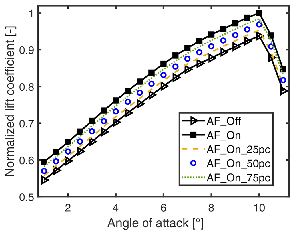
Figure 4 Example of flap normalized lift coefficient of the baseline (AF_Off, line with triangle); flap active (AF_On, line with squares); and flap active with performance reduced to 25 % (AF_On_25pc, dashed line), 50 % (AF_On_50pc, circles), and 75 % (AF_On_75pc, dotted line).

For every AFlap health state computed in the NPP case, we make two simulation sets: a training and test (TaT) set of 1000 simulations and a validation (Val) set of 500 simulations. The TaT sets cover a wind speed range from 3.5 to 25 m s⁻¹ and share the same sample set of environmental conditions. The Val sets cover the same wind speeds as the TaT sets but share a set of environmental conditions uncorrelated to the TaT set. The PS cases have a similar setup, but they cover wind speeds between 1 and 3.5 m s⁻¹; TaT sets have 300 simulations and the Val sets 150. Environmental condition sets used for the PS simulations are also uncorrelated to the NPP ones.

As the input of the ML model, we selected only signals commonly available in the modern commercial wind turbines. These signals are the pitch angle [^∘], the rotor speed [rpm], the generator power [kW], flapwise and edgewise bending moments at the root of each of the three blades [kNm], and linear tower top accelerations [m s⁻²], together with the flap actuator control signal [logic].

3 AFlap health state estimation with ML

3.1 Introduction

This paper investigates whether a simple ML algorithm can estimate the health state of an active trailing edge flap from the data provided by the sensors commonly available on a commercial WT. We approached this task as a multivariate time-series classification problem where the ML algorithm aims to estimate the AFlap health state. We followed two different approaches for computing the features from the sensors' time-series data. The first approach relies on the manual selection of the channels and their relevant statistics that, from the authors' knowledge, are known to be impacted by the trailing edge flap system. In contrast, the second approach relies on thousands of randomly generated convolutional kernels to generate the features from all the available signals. Based on the MiniRocket (MINImally RandOm Convolutional KErnel Transform) algorithm, this approach does not require pre-knowledge of the AFlap system's impact on the WT signals. It explores possible unknown correlations between the AFlaps states and the WT channels. As a classifier method, we selected the simple but robust random forest classifier for both feature calculation approaches. For the approach based on the MiniRocket algorithm, we also used the ridge classifier with cross-validation.

3.1.1 Random forest

A random forest classifier (RF) is a supervised discriminative machine learning technique whose objective is to estimate $P(Y\mid X,\mathit{\theta })$, in which Y is the target, X is the observable, and θ are the parameters. We assume a multi-class classification problem where each observational sample is assigned to one and only one label, as opposed to the multi-label approach.

The random forest classifier is based on a collection of decision trees (also called classification or prediction trees), a non-parametric supervised learning method designed for the classification or regression of a discrete category from the data. In the machine learning sense, the goal is to create a classification model (classification tree) that predicts the value of a target variable (also known as label or class) by learning simple decision rules inferred from the data features (also known as attributes or predictors). From Fig. 5a, an internal node N denotes a test on an attribute, an edge B represents an outcome of the test, and the leaf nodes L represent class labels or class distribution.

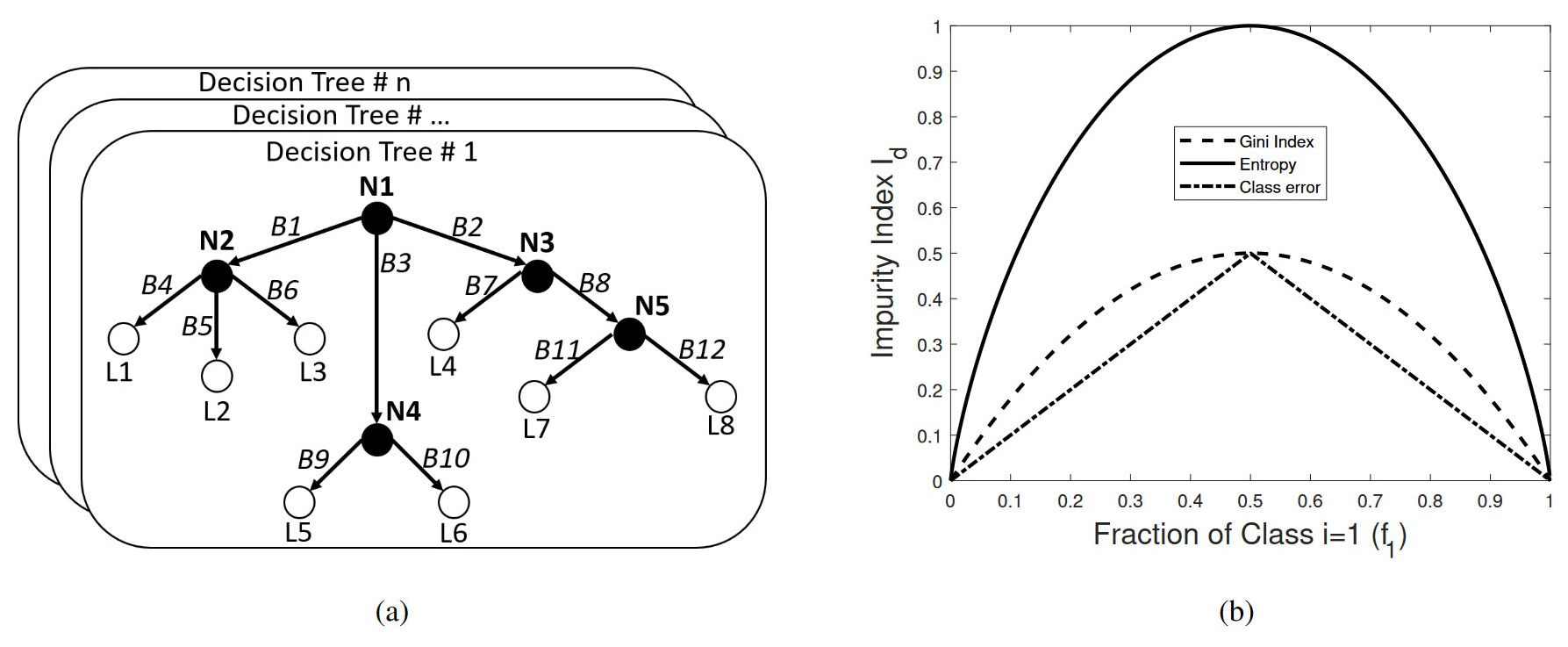
Figure 5 (a) Graphical representation of a forest of decision tree classifiers. (b) Impurity index I_d for a two-class example as a function of the probability of one of the classes f₁ using the information entropy, Gini impurity, and classification error. In all cases, the impurity is at its maximum when the fraction of data within a node with class 1 is 0.5 and is zero when all data are in the same category.

A decision tree is a tree-structured classifier built by starting with a single node that encompasses the entire data and recursively splits the data within a node, generally into two branches (some algorithms can perform “multiway” splits). The splitting is obtained by selecting the variable (dimension) that best classifies the samples according to a split criterion, i.e., the one that maximizes the information gain among the random subsample of dimensions obtained at every point. The splitting continues until a terminal leaf is created by meeting a stopping criterion, such as a minimum leaf size or a variance threshold. Each terminal leaf contains data that belongs to one or more classes. Within this leaf, a model is applied that provides a reasonably comprehensible prediction, especially in situations where many variables may exist that interact in a nonlinear manner, as is often the case with wind turbines (Carrasco Kind and Brunner, 2013). Several algorithms exist for training decision trees with variations on impurity, pruning, stopping criteria, how to treat missing variables, etc. A top-to-bottom construction of a decision tree begins with a set of objects. Each object has an assigned label and a set of measured features. The dataset is split at each tree node into two subsets, left and right, so the two resulting subsets are more homogeneous than the set in their parent node. To do so, one must define a cost function that the algorithm will minimize. One can use the information entropy, the Gini impurity, or a classification error for the cost function. Formally, the splitting is done by choosing the attribute that maximizes the information gain, defined in terms of the impurity degree index I_d as shown in Fig. 5b.

By definition, a random forest classifier is a non-parametric classification algorithm consisting of a collection of decision-tree-structured classifiers {h(x,Θ_k), k=1 … }, where Θ_k are independent identically distributed random vectors, and each tree casts a unit vote for the most popular class at input x. The RF prediction consists of the aggregation of the decision tree results obtained by a majority vote. Furthermore, the fraction of the trees that vote for the predicted class serves as a measure of certainty of the resulting prediction. Random forest improves prediction accuracy over single decision tree classifiers by injecting randomness that minimizes the correlation $\stackrel{\mathrm{‾}}{\mathit{\rho }}$ amongst the grown individual decision trees h(x,Θ_k) that operate as an ensemble. This is achieved by using bootstrap aggregating (a.k.a. bagging, sample with replacement of the training dataset) in tandem with random feature selection in the process of growing each decision tree in the ensemble (Breiman, 1996). This forces even more variation amongst the trees in the model (different conditions in their nodes and different overall structures) and ultimately results in lower correlation across trees and more diversification.

Some of the arguments in favor of using a random forest in this research include the following:

• Random forests work well with both categorical and numerical data. No scaling or transformation of variables is usually necessary.

• Random forests implicitly perform feature selection and generate uncorrelated decision trees. It does this by choosing a random set of features to build each decision tree. This also makes it a great model when you have to work with a high number of features in the data.

• Random forests are not influenced by outliers to a fair degree. It does this by binning the variables.

• Random forests can handle linear and nonlinear relationships well.

• Random forests generally provide high accuracy and balance the bias-variance trade-off well. Since the model’s principle is to average the results across the multiple decision trees it builds, it averages the variance as well.

• Random forests are fairly interpretable. They provide both feature importance and in certain instances the ability to trace branches to follow the decision-making process.

3.1.2 MiniRocket

Current methods for time-series classification often concentrate on singular aspects like shape, frequency, or variance. Convolutional kernels offer a unified approach capable of capturing multiple features that previously necessitated specialized techniques. These kernels have proven effective in convolutional neural networks for time-series classification like ResNet (Wang et al., 2017) and InceptionTime (Ismail Fawaz et al., 2020).

ROCKET (RandOm Convolutional KErnel Transform; Dempster et al., 2020) has demonstrated that achieving state-of-the-art classification accuracy is possible by transforming time series using random convolutional kernels. Unlike the learned convolutional kernels in conventional neural networks, Dempster et al. (2020) have shown that a combination of numerous random convolutional kernels can effectively capture relevant features for time-series classification. Even though a single random convolutional kernel might only approximate a relevant feature in a given time series, convolutional kernels significantly enhance the classification accuracy when combined. ROCKET is an algorithm that generates a large number of convolution kernels (10 000 by default) with random length, weights, bias, dilation, and padding of the time series provided as input. ROCKET extracts two features for each kernel: the maximum value (an equivalent to the maximum global pooling) and the proportion of positive values (PPVs), indicating the proportion of the input matching a given pattern. The PPV is the most critical element of ROCKET for achieving the state-of-the-art accuracy.

MiniRocket (MINImally RandOm Convolutional KErnel Transform) is a reformulated version of ROCKET (Dempster et al., 2021), 75 times faster while maintaining the same accuracy. MiniRocket minimizes the number of options for hyperparameters and computes only the PPV, generating half the number of features as ROCKET. In addition, it does not require normalization. The v0.3.4 version of the MiniRocket implementation in Oguiza (2022) has been used in this paper.

3.1.3 Ridge classifier with cross-validation

This ridge classifier uses the ridge regression to predict the class of a multiclass problem by solving the problem as a multi-output regression where the predicted class corresponds to the output with the highest value. Ridge regression, also known as Tikhonov regularization, solves a regression model by minimizing the following objective function:

$$\begin{array}{}\text{(7)}& {\min }_w\left|\right|Xw-y|{|}_{\mathrm{2}}^{\mathrm{2}}+\mathit{\alpha }|\left|w\right|{|}_{\mathrm{2}}^{\mathrm{2}},\end{array}$$

where X is the training data, y the target values, w the ridge coefficients to be minimized, and α the regularization strength; α controls the amount of shrinkage: the higher the value, the greater the amount of shrinkage, increasing the robustness of the ridge coefficients to collinearity. The addition of the cross-validation helps to identify the best set of ridge coefficients, reducing the risk of overfitting.

3.2 Manual feature selection (MFS) with random forest classifier

The main effect of the activation or deactivation of a trailing edge flap on a WT is the change in local blade lift that consequently affects the blade's aerodynamic loading. The impact on the blade loading depends significantly on the WT operative conditions, as shown in Gomez Gonzalez et al. (2022). Furthermore, asymmetric activation of the flaps on the three blades leads to a rotor bending moment imbalance that is often associated with tower top vibration. Based on this, we manually select a set of signals to generate the features to train an RF model. In addition, we consider only signals commonly available in all modern commercial wind turbines. The aim is the development of a method that can be implemented on commercial wind turbines without the need of installing additional hardware. Initially, we use simple statistical properties of the signal time series as features. Afterward, we include the catch22 (CAnonical Time-series CHaracteristics) collection (Lubba et al., 2019) to expand the features pool.

3.2.1 Signal and feature selection

The selected WT signals are as follows:

• flap actuator control signal [logic] – control signal of the flap activation state (on or off);

• flapwise and edgewise bending moments at the three blade roots [kN m⁻¹] – main signals to detect the impact of the flaps on the blade aerodynamic loading (load sensors placed at the blade root are commonly available in modern WTs);

• pitch angle [^∘], rotor speed [rpm], and generator power [kW] – main signals to estimate the WT's operative condition to which the flaps' load impact is related (these signals are available in every WT controller);

• fore–aft and side–side tower top accelerations [m s⁻²] – useful signals in detecting possible rotor imbalances (the WT safety systems commonly monitor these signals to detect WT anomalies);

• out-of-plane rotor bending moments [kN m⁻¹] – signals computed from the blade root moments, pitch angle, and azimuth position through the Coleman transformation Bir (2008) equation (these moments help detect possible rotor imbalances).

The initially selected features are the standard deviation, mean, maximum, minimum, range, and maximum absolute value of every signal. Afterward, we add the catch22 collection (Lubba et al., 2019) to expand the features pool to explore possible unknown correlations between the input signals. We choose the catch22 collection as it is a high-performing subset of 22 features selected over a pool of over 7000 based on their classification performance across a collection of 93 real-world time-series classification problems. The catch22 v0.4 MATLAB tool is used for this paper. Finally, we include the blade-to-blade difference between the mean and absolute maximum blade root bending moments to help detect possible flap activation imbalances.

The feature generation process computes circa 400 features for each aeroelastic simulation. To reduce complexity, we add two feature filtering processes to the algorithm:

• Manual selection of the desired feature subset in the algorithm pre-processing is the first.

• Automatic feature reduction based on out-of-bag permuted predictor importance (oobPPI) value is the second. The oobPPI measures how influential a feature is in the model prediction by permuting the value of the feature and measuring the model error. The permutation of an influential feature should have a relevant effect on the model error; little to no effect should come from a permutation of a non-influential feature. If this filter is active, the oobPPI of each feature is evaluated after the RF model is trained. Features with an oobPPI value below the threshold specified by the user are removed, and the RF model is trained again with the remaining feature subset. The process is repeated until all the remaining features consistently have an oobPPI value above the threshold, simplifying the final model by removing the features not influential on the classification process.

We decided to not include the wind speed sensor signal in the ML training. This sensor is generally located on the nacelle, behind the rotor, where the complexity of the 3D wind flow can only be correctly estimated by high-fidelity codes, like CFD. In this paper we use a mid-fidelity aeroelastic model that is unable to estimate the wind speed on the nacelle with sufficient accuracy. Therefore, training the ML model with a low-fidelity nacelle wind speed would reduce the model accuracy and performance on a real WT. Furthermore, the ML model can still derive the wind speed data from the rotor speed, pitch angle, and generator power, which strongly correlate to the wind speed. Therefore, omitting the wind speed signal reduces model uncertainties without losing relevant data for the ML training. Instead, we use the mean wind speed for splitting the NPP into different wind speed regions for which a dedicated RF model is trained. Generally, a modern WT operates differently below rated wind speed, where it is power or torque controlled, compared to above rated wind speed, where it is pitch controlled. Therefore, we expect RF models trained for each specific wind region to perform better than a single RF model covering the whole wind speed range.

3.2.2 Algorithm structure and setup

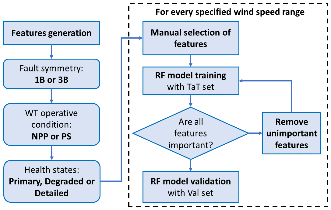
The algorithm structure, shown in Fig. 6, has the following steps:

1. calculation of the features for every simulation (usually it is done only once, after the aeroelastic simulation is computed);

2. selection of the AFlap fault symmetry (1B or 3B) and WT operative condition (NPP or PS);

3. selection of the AFlap health states to be used in the classification;

4. for every specified wind speed range,

   1. manual selection of the desired feature subset

   2. training of the RF model with the TaT set

   3. if the “automatic feature reduction” is enabled, the following steps are repeat until all features have oobPPI above threshold:

      1. evaluation of the oobPPI of every features

      2. removal of the features with oobPPI below threshold

      3. training of a new RF model with the remaining features

   4. validation of the trained RF model with the Val sets.

Figure 6 Schematic structure of MFS algorithm.

In the algorithms, three MATLAB functions are used: templateTree to create the decision tree template, fitcensemble to train the RF model, and oobPermutedPredictorImportance to compute the oobPPI value for each feature.

We use the setup proposed by Abdallah (2019) as the default RF setup: number of trees of 100, learning rate of 0.25, maximum number of splits of 12, test rate of 30 %, and oobPPI threshold of 0.01.

3.3 Automatic feature generation with random forest or ridge classifier

The automatic feature selection (AFS) approach relies on the same signals used for the manual feature selection approach: pitch position, rotor speed, generator power, flapwise and edgewise bending moments at the root of each of the three blades, linear tower top accelerations, and the flap actuator control signal. As described in Sect. 3.2, these signals are relevant to detect the flap impact on the WT and are provided with the standard sensors available on commercial WTs. Instead of generating a set of features for each signal based on statistical properties, the AFS approach utilizes ML techniques developed for image processing to create features of the whole simulation. We implement two different algorithms for the classification: a RF classifier, similar to what we used for the MFS, and a ridge classifier with cross-validation (ridge) suggested by Dempster et al. (2020) for application with MiniRocket.

3.3.1 Feature generation with MiniRocket

MiniRocket works by first combining the time series of the relevant signals of a single simulation in a single matrix, aligning them as a function of time. Then it processes the resulting matrix like an image utilizing a kernel from which the proportion of positive values is computed. A set of 10 000 kernels of random lengths, weights, bias, dilation, and padding are used, generating 10 000 features per simulation. This process is repeated for all the simulations. For consistency, the same kernel set must be used for all the simulations used in the RF models' training, testing, and validation.

3.3.2 Algorithm structure and setup

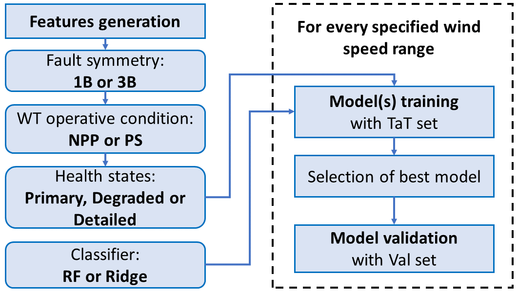
The algorithm structure, shown in Fig. 7, has the following steps:

1. calculation of the features with MiniRocket

2. selection of the AFlap fault symmetry (1B or 3B) and WT operative condition (NPP or PS)

3. selection of the AFlap health states to be used in the classification

4. selection of the classifier: RF or ridge

5. for every specified wind speed range,

   1. training of the classification model:

      1. training of one (or more) classification model

      2. if more than one classification model is trained, select the model with higher F1 score

   2. validation of the trained classification model with the Val sets.

Figure 7 Schematic structure of AFS algorithm.

In the AFS method, we used the following sklearn Python codes (Pedregosa et al., 2011): StratifiedShuffleSplit to create multiple test and training subsets from the TaT sets; RandomForestClassifier to train, test, and validate the RF models; RidgeClassifierCV to train, test, and validate the ridge classifier models; f1_score to compute the F1 score; and StandardScaler to standardize features by removing the mean and scaling to unit variance.

Starting from the setup proposed by Abdallah (2019), we investigate the optimal RF setup for the different scenarios, obtaining as optimal values a test rate of 30 %, number of trees of 100, Shannon entropy as the criterion to measure the quality of a split, maximum depth of the tree of 5, minimum number of samples required to split an internal node of 5, and all features included.

For the ridge setup, the regularization strength parameter was set to an evenly spaced vector in log space of 1000 values between 1 and 10⁶ and the cross-validation set to leave-one-out cross-validation that handles efficiently the case of the number of features higher than the number of samples.

4 Manual feature selection results

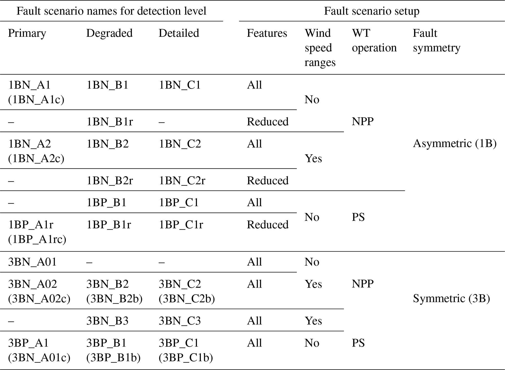
The potential of the MFS approach in detecting a flap system's fault is investigated for several AFlap fault scenarios. These scenarios cover different combinations of AFlap fault symmetries (1B or 3B), WT operative conditions (NPP or PS), the possible split in different wind speed ranges, and different initial feature selection (all or reduced). The initial feature option allows the reduction in the features used in training. We set the feature subset without the catch22 collection as the default reduced setup. Instead, the wind speed range option enables the training of a dedicated ML model for every specified wind speed range. The default ranges used in this paper are below rated (BR: wind speed between 3.5 and 9.5 m s⁻¹), around rated (Rt: wind speed between 9.5 and 16.5 m s⁻¹), and above rated (AR: wind speed between 16.5 to 25 m s⁻¹).

Furthermore, we investigate three different fault detection levels.

• Primary. The model is trained to detect only the four primary health states: flap not active (AF_Off), active (AF_On), not active with fault (AF_Off_Fault), and active with fault (AF_On_Fault).

• Degraded. The model is trained to detect if the flap has degraded performance but without identifying the performance degradation level. The three health states of flap with degraded performance are merged in a single state, called active with degradation (AF_On_Degr), that is included in the training with the four primary health states.

• Detailed. The model is trained to identify the flap performance reduced to 25 % (AF_On_25pc), 50 % (AF_On_50pc), and 75 % (AF_On_75pc) in addition to the primary health states.

Table 2 collects the list of the MFS scenarios and shows their setup. Scenarios stated within parenthesis have a customized setup detailed described in the following chapters.

Table 2 Compact description of the setup of the AFlap fault scenarios.

The selection of the models' performance metrics is strictly related to the requirements of the detection system. If one (or more) flap fault is critical for the WT integrity, the detection of this fault would be prioritized over the other AFlap health states. In this case, a good metric would be the recall of the critical fault. For an opposite scenario, where it would be more critical to avoid false fault detections and keep the WT operating, the precision of the different faults should be considered. In this paper, we are not considering any particular requirement for the fault detection system, and we aim to correctly detect all the different classes equally without prioritizing any one specifically. Therefore, we select the F1 score, a trade-off between recall and precision that rewards the reduction in both false positives and false negatives. In detail, we use the weighted F1 score: the average of the F1 score of each class weighted by the ratio of the number of samples of each class over the total sample number. This metric is consistent between balanced and unbalanced classification tasks, allowing us to evaluate the few scenarios where the classes are not balanced.

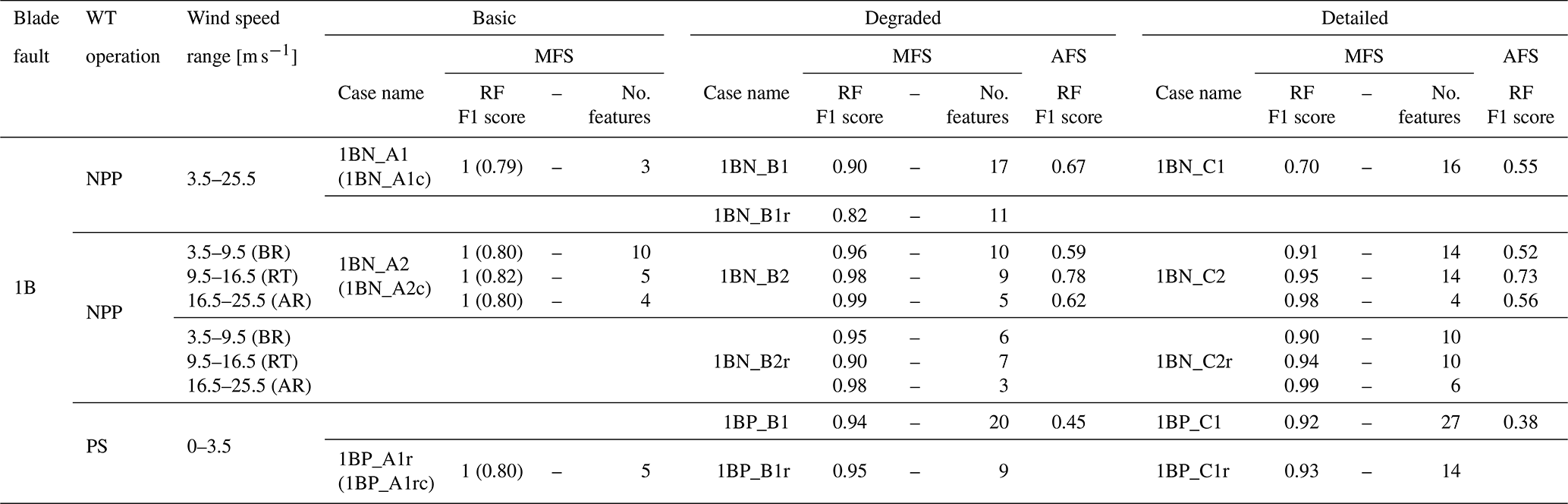
Table 3 F1 score of the asymmetric flap fault scenarios evaluated with MFS and AFS approaches. The number of features used for the MFS is also specified.

4.1 Detection of asymmetric fault

Table 3 collects the performance of the RF models trained for the asymmetric fault scenarios described in Table 2. In addition to the weighted F1 score, the number of features obtained after the automatic feature reduction in the model training is shown. We use this number as an estimate of the model complexity: where more features are needed, it is more complex to implement and execute the model. In addition, precision and recall values of the AFlap health states for some specific asymmetric fault scenario models are collected in Table 4.

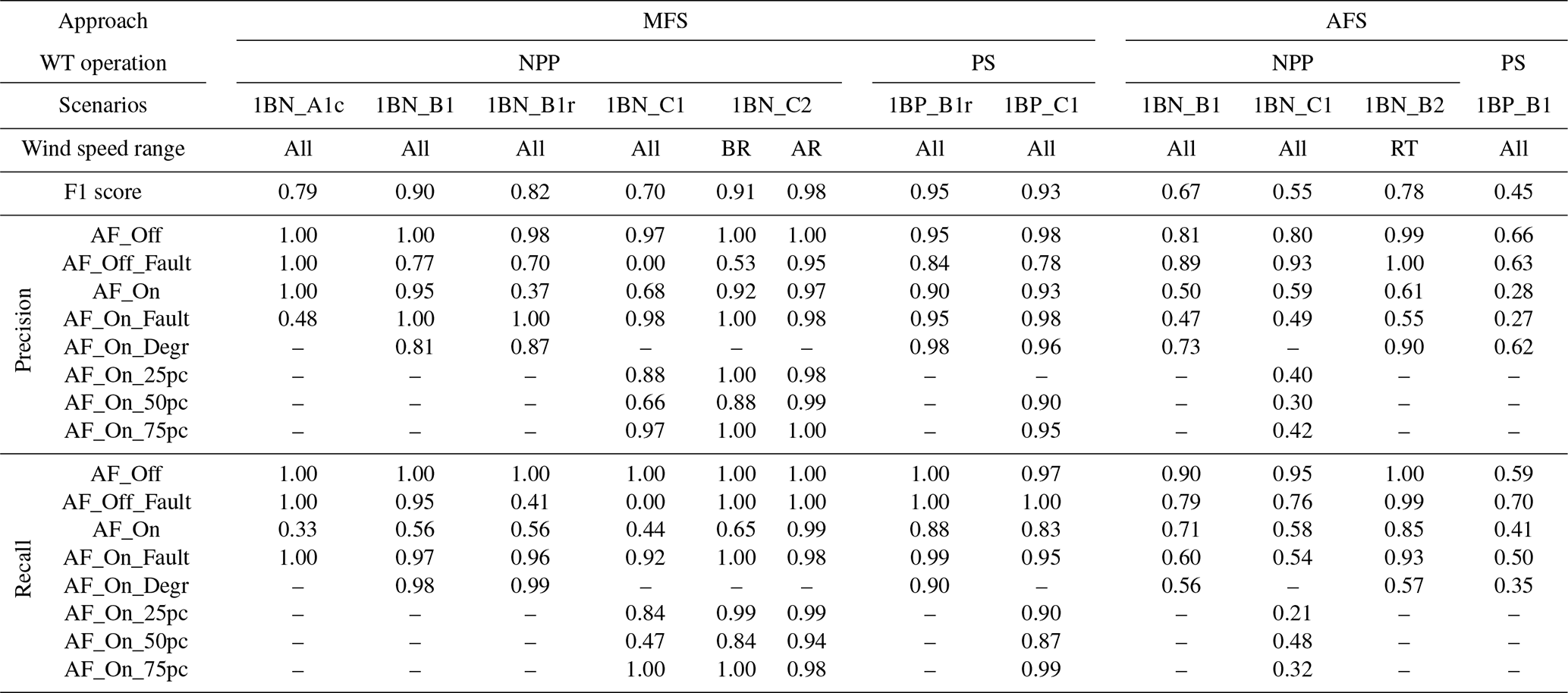
As the first step, scenario 1BN_A1 trains a single RF model for all the wind speeds to detect the primary flap health states in normal power production, starting the training with all the available features. The trained model needs only three features (out of 400) to achieve an F1 score of 1, meaning it can perfectly classify the primary health states. To understand how this trained model would perform with AFlap degradation (which will occur during the normal lifetime of the flap, also as a partial fault), we evaluate it with all the degraded AFlap health states classified as AF_On_Fault (scenario 1BN_A1c). Under this condition, the model F1 score decreases to 0.79 due to the misclassification of the flap fault (AF_On_Fault) as normal flap operation (AF_On). This misclassification is expressed numerically by a low value of AF_On recall (0.33) and AF_On_Fault precision (0.48). We obtain comparable results in scenario 1BN_A2, where the wind speeds are split into three different wind speed ranges, and an independent RF model is trained for each range. The models trained in this scenario detect well the primary health states (F1 score of 1) but cannot distinguish the degraded AFlap states (scenario 1BN_A2c).

As the second step, we unify the degraded AFlap health states under a single category (AF_On_Degr). Scenario 1BN_B1 trains a single RF model for all the wind speeds to detect the degraded fault health states in NPP. The trained model requires 17 features for an F1 score of 0.90 mainly due to the low recall (0.56) of the AF_On class. Removing the catch22 features to simplify the model (scenario 1BN_B1r) leads to a lower F1 score (0.82), poor AF_Off_Fault class recall (0.41), and poor AF_On class precision (0.37). Splitting the training for the tree wind speed ranges (scenario 1BN_B2) generates three high-performing models (F1 score higher than 0.95) even in the scenario where the catch22 features are removed (1BN_B2r).

As the last step for the NPP case, we evaluate if a model could individually identify the degraded AFlap health states. Scenario 1BN_c1 trains a single RF model for all the wind speeds for a detailed detection level in NPP. The trained model requires 16 features for an F1 score of 0.70 and can almost not distinguish the AF_Off_Fault from the other classes. Splitting the training for the tree wind speed ranges (scenario 1BN_c2) dramatically improves the performance of the models with an F1 score of 0.91 BR, 0.95 Rt, and 0.98 AR obtained with 14 features or less. In detail, the BR model is imprecise in classifying the AF_Off_Fault and has a low recall for AF_On. Removing the catch22 features leads to models with similar performance but fewer features (10 or less).

Table 4 Precision and recall values of each AFlap health state of a selection of scenarios of asymmetric flap fault evaluated with MFS and AFS approaches.

After the NPP scenarios, we investigated if the AFlap health states can be correctly classified in pre-startup conditions where the WT is idling due to low wind speed. For the scenarios aiming at the primary flap health states (1BP_A1r and 1BP_A1rc) in the PS condition, the performance follows the same pattern as the previous similar scenarios in NPP. When the AF_On_Degr class is included (scenario 1BP_B1), the trained model shows a high F1 score (0.94) with 20 features. A high F1 score of 0.95 is also achieved with only nine features starting from a reduced set of features (scenario 1BP_B1r). Finally, when we analyze the detailed detection level (scenario 1BP_C1), the trained model achieves an F1 score of 0.92 with 27 features. Omitting the catch22 features in training (scenario 1BP_C1r) brings an equivalent F1 score with only 14 features.

4.2 Detection of symmetric fault

Table 5 collects the performance of the RF models trained for the symmetric fault scenarios described in Table 2. Precision and recall values of the AFlap health states for some specific symmetric fault scenario models are collected in Table 6.

Table 5 F1 score of the symmetric flap fault scenarios evaluated with MFS and AFS approaches. The number of features used for the MFS is also specified.

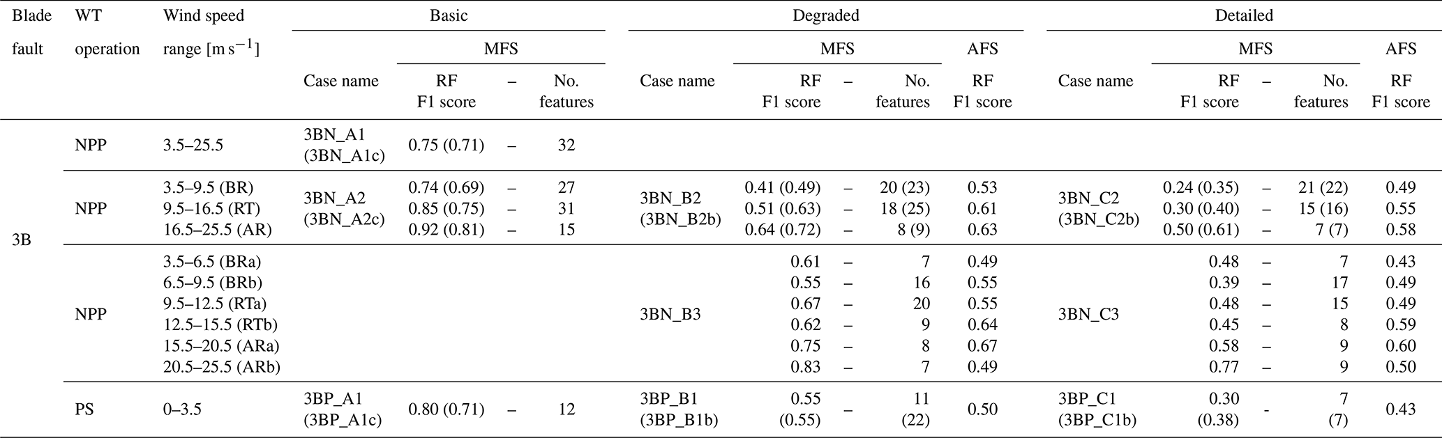
Table 6 Precision and recall values of each AFlap health state of a selection of scenarios of symmetric flap fault evaluated with MFS and AFS approaches.

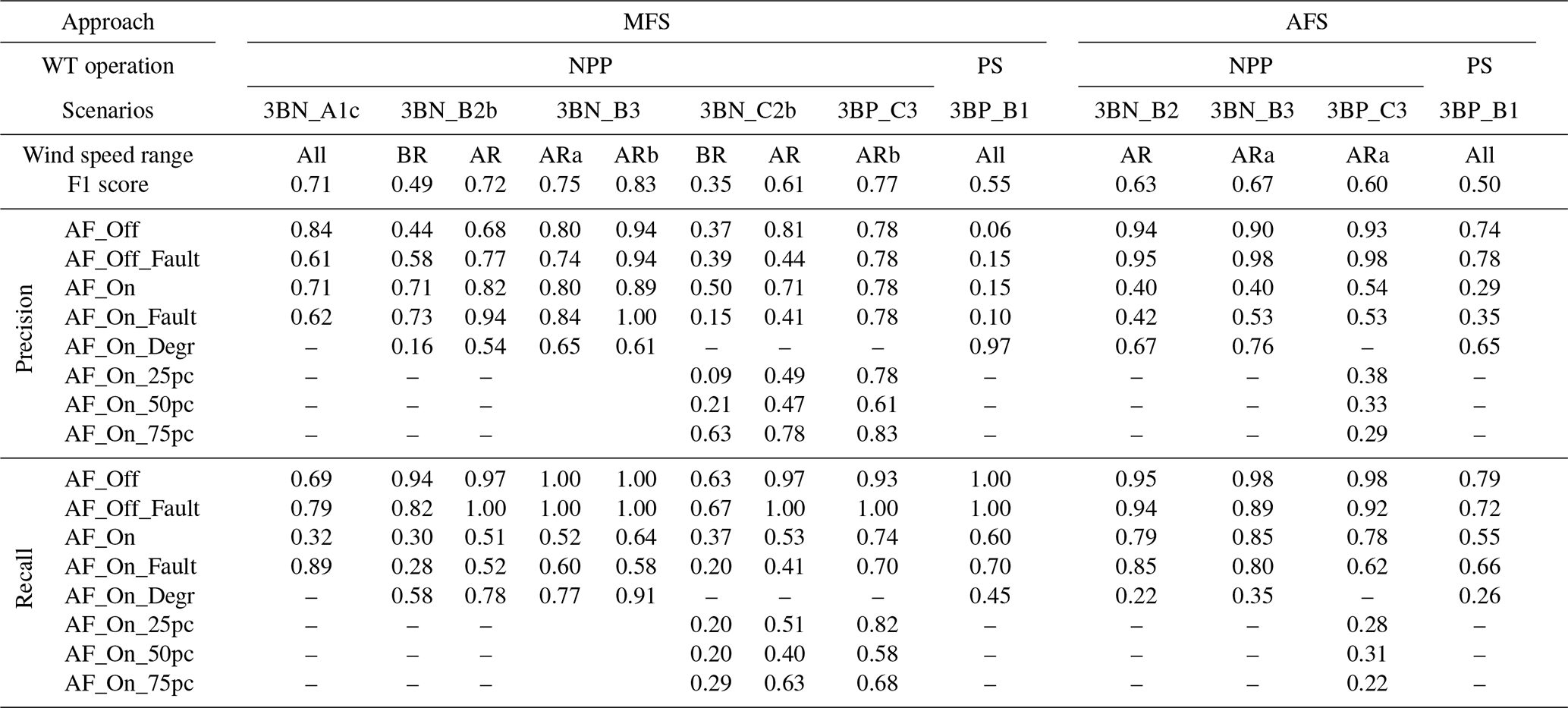
Similar to the asymmetric faults' cases, we start with a scenario (3BN_A1) that trains a single RF model for all the wind speeds to detect the primary health cases in NPP, using all the available features initially. The trained model achieves an F1 score of 0.75 with 32 features. When tested with the degraded flap health states bundled together as AF_On_Fault (scenario 3BN_A1c), the F1 score decreased to 0.71 due to the misclassification of the fault (AF_On_Fault) as normal flap operation (AF_On). This misclassification is expressed numerically by a low value of AF_On recall (0.33) and low precision (0.61) of both AF_Off_Fault and AF_On_Fault. We obtained comparable results in scenario 3BN_A2, where we trained an independent RF model for each of the three different wind speed ranges. The models trained in this scenario detect better than the previous scenario the primary flap health states, especially for AR (F1 score of 0.92), but cannot correctly distinguish the degraded AFlap states (scenario 1BN_A2c).

As the second step, we include the degraded AFlap health states under a single category (AF_On_Degr). Scenario 3BN_B2 trains an independent RF model to detect the degraded flap cases in NPP for each of the three different wind speed ranges. The trained model shows a low F1 score of 0.41 for BR, 0.51 at rated, and 0.64 for AR. To improve the performance of the models, we explore the RF model hyperparameter setup. One of the most successful results is scenario 3BN_B2b, where we increase the number of trees from 100 to 300 and the maximum number of slits from 12 to 30. These changes lead to an increase in the F1 score by around 0.08, with the highest value achieved in the AR wind speed range with an F1 score of 0.72. This model still shows low recall for AF_On and AF_On_Fault flap states and a low precision for AF_On_Degr. As a final try to increase the models' performance, we reduce the width of the wind speed ranges, obtaining BRa (3.5 to 6.5 m s⁻¹), BRb (6.5 to 9.5 m s⁻¹), RTa (9.5 to 12.5 m s⁻¹), RTb (12.5 to 15.5 m s⁻¹), ARa (15.5 to 20.5 m s⁻¹), and ARb (20.5 to 25.5 m s⁻¹). This scenario (3BN_B3) leads to RF models with higher performance, but only ARa and ARb models have the F1 scores higher than 0.7 (0.75 and 0.83, respectively). Both RF models have good precision except for the AF_On_Degr class but a low recall for AF_On, AF_On_Fault, and AF_On_Degr.

Finally, we investigate if an RF model could individually identify the detailed flap health states, obtaining models with poor performance in the symmetric fault case during NPP. Scenario 3BN_C2 trains an independent RF model to detect the degraded fault cases in NPP for each of the three different wind speed ranges. The trained model has an F1 score below 0.50. Increasing the number of trees to 300 and the maximum number of slits to 30 (scenario 3BN_C2b) improves the F1 score of around 0.1. The precision and recall values show that the models cannot correctly detect most AFlap health states. Adding the reduction in the size of the wind ranges (scenario 3BN_C3) does slightly improve the F1 score but with the best-performing model (ARb) reaching only an F1 score of 0.77. For the PS wind turbine operation, the scenario aiming at the degraded flap health states (scenario 3BP_B1) trains a model with a low F1 score (0.55) but is unable to classify all the different AFlap health states correctly. Increasing the number of trees and split (3BP_B1b) does not lead to better performance. Also, for the detailed detection level (scenario 3BP_C1), the trained model achieves a poor F1 score of 0.30 that is only marginally improved (0.38) by increasing the number of trees and split (3BP_C1b).

5 Automatic feature selection results

The AFS approach is investigated with most of the scenarios used for the MFS approach and collected in Table 2. An initial preliminary investigation shows that a model trained only to detect the primary flap health states will most likely perform poorly when the AFlap starts to have degraded performance, similar to what we obtain in the MFS analysis. Since this performance degradation is likely to happen, there is a low interest in a model that cannot account for it properly, and the primary fault detection level is therefore omitted in the AFS analyses. Furthermore, the initial feature reduction does not apply to the AFS approach, and the scenarios with the reduced feature setup are not included. Regarding the RF hyperparameter setup, we ran an initial study using several randomly generated subsets of features to identify the values of the hyperparameters optimizing the F1 score. This study shows an optimal hyperparameter setup with the number of trees being 100 (an increase up to 300 does not improve the performance), the maximum depth of the tree being 5 (lower values tend to cause overfitting), the minimum number of samples required to split an internal node being 5, and Shannon entropy as a criterion to measure the quality of a split. The final model training is instead performed including all the features. This configuration showed better performance compared to the random pick of a subset of features of the size of square root or log ₂ of the total number of features.

Having a number of features considerably higher than the number of samples, a condition not ideal for the RF method, we investigate if another classifier can perform better than RF. We selected the ridge regression classifier with cross-validation, a linear classifier tested in the development of both ROCKET (Dempster et al., 2020) and MiniRocket (Dempster et al., 2021).

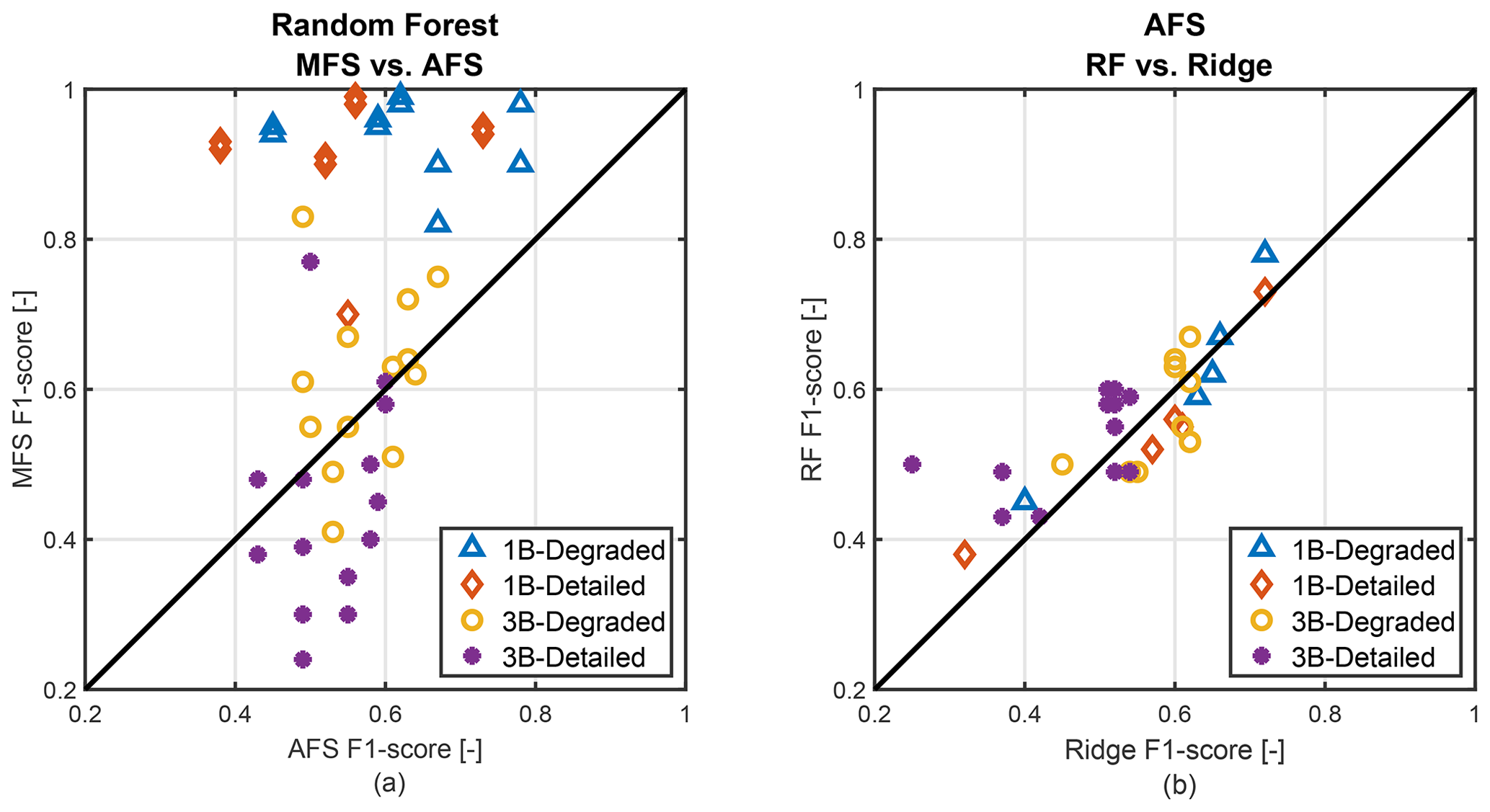
Figure 8 (a) Comparison between the MFS RF F1 scores and the MFS RF F1 scores of the different degraded and detailed flap health scenarios. (b) Comparison between the AFS RF F1 scores and the AFS ridge F1 scores of the different degraded and detailed flap health scenarios.

5.1 Detection of asymmetric fault

The performances of models trained with the RF classifier for the asymmetric fault scenarios described in Table 2 are shown in Table 3, together with the results from the MFS approach. Table 4 collects precision and recall values of the AFlap health states for some specific asymmetric fault scenarios of the RF models.

In NPP, AFS RF shows low performance when trained to detect the degraded health states for all the wind speeds (scenario 1BN_B1) with an F1 score of 0.67. The model can correctly classify the AF_Off and AF_Off_Fault states but cannot classify the other AFlap health states, as indicated by the recall and precision values. When we train the classifiers for the detailed health states (scenario 1BN_C1), performance decreases with an F1 score of 0.55. Also, for this scenario, the models can adequately classify AF_Off and AF_Off_Fault states but fail with the other states. Performances slightly increase when we split the training into different wind speed ranges. AFS RF achieves the highest performance in evaluating the degraded health states (scenario 1BN_B2) around rated wind speed with an F1 score of 0.78. For the other wind speed ranges, the F1 score stays around 0.6. Comparable results are achieved for the detailed health states (scenario 1BN_C2), where AFS RF achieves a max F1 score of 0.73 at RT but not higher than 0.56 in the other wind speed ranges. Looking at the results in PS, the RF classifier performs poorly in identifying degraded and detailed health states (scenario 1BP_B1 and 1BP_C1, respectively) with a max F1 score of 0.45.

Figure 8 compares the F1 scores from AFS RF with the scores from AFS ridge. The ridge classifier achieves results comparable to RF for degraded and detailed flap health states in the 1B case. Also, the precision and recall values of the ridge models are close to the values of the RF models of the corresponding scenarios. For brevity, we have not included them in this paper.

5.2 Detection of symmetric fault

The performances of models trained with the RF classifier for the symmetric fault scenarios described in Table 2 are shown in Table 5, together with the results from the MFS approach. Precision and recall values of the AFlap health states for some specific asymmetric fault scenario models are collected in Table 6.

In NPP, AFS RF shows low performance when trained to detect the degraded health states (scenario 3BN_B2) for different wind speed ranges. The F1 score is between 0.53 at BR and 0.63 at AR. Similar to what was observed in the asymmetric fault, the models can detect most of the AF_Off and AF_Off_Fault states properly but cannot classify the other AFlap health states. Reducing the width of the wind speed ranges (scenario 3BN_B3) mainly reduces the performance, especially for low and high wind speeds, except at ARa, where the F1 score increases up to 0.67. Looking at the detailed health states for the three wind seed ranges (scenario 3BN_C2), the F1 score rises from 0.49 at BR to 0.58 at AR. Similar to the degraded flap health states, reducing the width of the wind speed ranges (scenario 3BN_C3) does reduce the performance, especially for low or high wind speeds. Like the previous scenarios, the models have high recall and precision values for AF_Off and AF_Off_Fault states and low values for the other health states.

Looking at the results in PS, AFS RF classifiers perform poorly in identifying degraded and detailed health states (scenario 1BP_B1 and 1BP_C1, respectively) with a max F1 score of 0.5. Also, the ability to correctly classify AF_Off and AF_Off_Fault states is consistently reduced with both recall and precision below 0.8.

Similar to the asymmetrical case, the ridge classifier achieves comparable results to RF for both degraded and detailed flap health states in the 3B case. Figure 8 shows that AFS RF performs slightly better than the ridge classifier for the detailed flap health states.

6 Discussion

6.1 Manual feature selection with random forest

The results described in Sect. 4.1 show that the manual feature selection approach with a random forest classifier can correctly classify the AFlap health states in the case of asymmetric flap fault 1B. In normal power production, degraded and detailed health states are correctly classified, and the performance increases when splitting the training into three wind speed ranges. This result supports our initial hypothesis that as a WT operates differently at different wind speed ranges, models trained for specific wind ranges perform better than a single model trained for all wind speeds. Notably, less than 20 features are needed for the models, a small fraction of the around 400 provided at the beginning of the training. This number can be further reduced to 10 or fewer by removing the catch22 features without significantly reducing the models' performance. Even if few features are specific to some scenarios, all scenarios share the blade-to-blade differences between the mean blade root bending moment (mainly of flapwise bending moment), followed by the mean value of WT performance indicators like pitch angle, generator power, rotor speed, or blade root bending moments. This sounds logical since an asymmetrical flap fault among the different blades should result in a relevant difference in the blades' loading. The blade-to-blade load difference channels should collect this load imbalance. Furthermore, the blade imbalance is a function of the WT operational working state that the models most probably identify with the WT performance indicator features. Also, the models need fewer features at above rated wind speed, where generator power and rotor speed are almost constant, and the blade-to-blade load difference is most likely less impacted by them. Looking at the pre-startup operation, both degraded and detailed health states are correctly classified and the catch22 features can be omitted without reducing performance, as experienced in NPP. The models need more features than the NPP scenarios, still with blade-to-blade load difference as the key feature followed by mean values of the blade loads. Generator power and rotor speed are no longer relevant, being almost null in the idling state.

Regarding the primary health states detection, the models obtained with MFS show, on one side, high performance in identifying the four primary health states in both NPP and PS, but on the other side, they cannot account properly for the degradation of the AFlap performance. Since this degradation is likely to happen in the WT lifetime, we think these models can lead to some significant misclassification, and we do not recommend them for field application.

In the case of a symmetric flap fault 3B, the MFS approach fails to correctly classify all the tested AFlap health states in both NPP and PS operation states. Increasing the model complexity or reducing the wind range width improves the performance negligibly, and the only case with an acceptable F1 score is the degraded health states at high wind speeds (ARb). Looking at the selected features helps to understand the reasons for the misclassification. The blade-to-blade features are no longer present, replaced by several features related to single-blade loading, tower top accelerations, and rotor speed. This result confirms that the blade-to-blade loads no longer contain any flap fault information in the symmetric fault scenario, where the flap fails symmetrically in all three blades. Therefore, the RF models try to estimate the AFlap health states from the features of other channels, like blade loads. The failure to obtain satisfactory performance means the channels used in training do not have sufficient information to identify the AFlap health states, and more signals are needed to achieve it. A possible solution to properly detect and classify AFlap health states in the 3B condition is to transform it into an asymmetrical case. This transformation can be achieved with a flap check routine that activates the flap one blade at a time, which is like a 1B condition where the RF models can accurately estimate the flap health states.

The reduced feature set of the MFS approach relies on statistical data commonly available in the commercial wind turbine SCADA data. This approach greatly facilitates the application of this methodology to commercial wind turbines. To do so, the MFS model must be trained with simulations based on the target wind turbine aeroelastic model and eventually fine-tuned with transfer learning techniques using the wind turbine SCADA data. Instead, the MFS method with full feature requires calculating additional features generally not included in the standard SCADA data. For this method, a cost–benefit evaluation should identify which features are relevant to be computed in addition to the standard SCADA data.

6.2 Automatic feature selection with random forest and ridge classifier

The results described in Sect. 5 show that the automatic feature selection approach with a random forest classifier cannot correctly classify the AFlap health states for both asymmetric and symmetric flap fault cases. The trained models do not reach an F1 score higher than 0.8 in 1B scenarios and higher than 0.7 in 3B scenarios. Figure 8 compares the F1 scores between MFS and AFS RF models, with the MFS models outperforming the AFS models in the 1B scenarios. In the 3B scenarios, AFS RF models perform slightly better, especially for the detailed flap health states. As shown in Fig. 8, for the 1B scenarios, AFS ridge models perform similarly to the AFS RF models in 1B cases and slightly worse in the 3B cases. The overall performances of the AFS models need to be further improved before the AFS models can be implemented in detecting all the AFlap health states. However, the AFS models performed better than the MFS models for two flap health states. For the NPP operation state, the AFS models can correctly identify the AF_Off and AF_OFF_Fault flap health states from the other states with precision and recall above 0.9. This result suggests that the selected input channels also carry the flap state information for the NPP state. The AFS method has the potential to detect this information, even if partially, for the flap state estimation. Further studies are needed to achieve acceptable precision and recall for all the flap health states. These studies should cover a comprehensive study on the impact of the different setup parameters on the model performance or explore other ML techniques like, for example, MultiRocket (MiniRocket evolution) or HYDRA.

Regarding the implementation in the wind turbine controller, the AFS approach processes the whole 10 min signal data to generate the features. Therefore, it requires a dedicated feature generation algorithm that computes the features constantly. As a result, implementing the AFS requires more resources (both hardware and software) than the MFS.

7 Conclusions

The integration of active flaps in the wind turbine design has the potential to reduce loads and enhance wind turbine performances. However, this integration requires implementing systems to detect, monitor, and quantify any potential fault or performance degradation of the flap system to avoid jeopardizing the wind turbine's safety and performance. This paper investigated two approaches to identify the health state of a WT's active trailing edge flaps. These approaches do not rely on specific sensors designated for AFlap's health monitoring but only on sensors commonly available on all commercial wind turbines. Both approaches are based on multivariate time-series classification methods. The first method (MFS) uses manual feature engineering in combination with a random forest classifier. The second method (AFS) creates the feature vectors from multivariate time-series data by passing the inputs through multiple random convolutional kernels in combination with a random forest classifier. We trained both methods to classify combinations of seven AFlap health states for a WT operating in normal power production and pre-startup. We analyzed asymmetrical flap faults, with the flap health states applied to only one blade, and symmetrical flap faults, where the flap health states were applied to all three blades. The study is based on a pool of aeroelastic simulations of a WT equipped with an active flap. These simulations were performed with a broad set of environmental conditions to account for the variability due to external weather conditions in the model's training. To keep the approach as general as possible, we focused on identifying the AFlap health state when the flap is in stationary actuation positions. This approach keeps the detection system independent from any specific AFlap controller strategy, AFlap system design, or fault dynamics. The underlying idea is to integrate the monitoring system in an AFlap status check routine running for several minutes where the performance of the stationary flap is verified.

In this paper, we showed that the MFS method could classify the different combinations of AFlap health states in the case of asymmetrical flap faults. The MFS method is reliable when the WT operates in normal power production and pre-startup, achieving an F1 score higher than 0.9. Essential features to achieve this result are the blade-to-blade differences in the mean blade root loads.

Instead, the MFS method failed to classify the AFlap health states in the case of symmetrical flap fault. This failure is likely due to the channels used for the training not providing sufficient information about the flap fault. To avoid adding other sensor signals to the model, we suggest transforming the symmetrical flap fault detection into an asymmetrical one. For example, a flap check routine can activate the flap one blade at a time, generating a temporary asymmetrical flap activation that the MFS methodology can monitor.

As the MFS approach with a reduced feature set relies only on 10 min statistical properties, we believe it can be directly implemented in an actual wind turbine. The model must be trained with simulations based on the target wind turbine aeroelastic model and eventually tuned with transfer learning techniques using the wind turbine SCADA data. Instead, the MFS method with full feature requires calculating additional features generally not included in the standard SCADA data. For this method, a cost–benefit evaluation should be performed to identify which features are relevant to be computed in addition to the SCADA data.

Furthermore, we showed that, in general, the AFS method fails to classify most AFlap health states in asymmetrical and symmetrical flap faults. However, AFS can identify some specific flap health states better than the MFS method for the symmetrical case. This result suggests that the selected input channels carry the flap state information for the NPP state, but only the AFS method has the potential to detect them. We also evaluated a ridge classifier in the AFS method, obtaining a similar performance to the random forest classifier with a consistently lower training time.

Compared to the MFS approach, implementing the AFS method will require more resources as it needs additional preprocessing to generate the features. The methodologies described in this study contribute to developing the systems for detecting and monitoring active flap faults, which are paramount for the safe and reliable integration of active flap technology in future wind turbine design.

As future developments, we suggest further exploring the AFS method by applying different and better performing convolutional techniques. Also, the AFS and MFS methodology can be combined into a hybrid system to investigate if the combined system presents improved performances by leveraging the strengths of each method. It is also of extreme interest to validate the capability of the MFS method with data from an actual wind turbine, to which the models can be adapted via transfer learning techniques.

Appendix A: List of symbols

Flap states
AF_On	AFlap active without performance
	degradation
AF_Off	AFlap not activated
AF_On_Fault	AFlap not active due to fault
AF_Off_Fault	AFlap active due to fault
AF_On_25pc	AFlap active with performance reduced
	to 25 %
AF_On_50pc	AFlap active with performance reduced
	to 50 %
AF_On_75pc	AFlap active with performance reduced
	to 75 %
AF_On_Degr	Combination of all AFlap active with
	reduced performance
Fault scenarios
3B	Symmetrical AFlap fault
1B	Asymmetrical AFlap fault
NPP	Normal power production
PS	Pre-startup
BR	Below rated: wind speed ranges
	between 3.5 and 9.5 m s−1
Rt	Around rated: wind speed ranges
	between 9.5 and 16.5 m s−1
AR	Above rated: wind speed ranges
	between 16.5 and 25 m s−1
Other symbols
AFlap	Active trailing edge flap
WT	Wind turbine
pWT	Prototype wind turbine
ML	Machine learning
RF	Random forest classifier
TaT	Training and test set
Val	Validation set
oobPPI	Out-of-bag permuted predictor
	importance