the Creative Commons Attribution 4.0 License.
the Creative Commons Attribution 4.0 License.
 | 10 Sep 2024
Aerodynamic effects of leading-edge erosion in wind farm flow modeling
Tuhfe Göçmen
Özge Sinem Özçakmak
Alexander Meyer Forsting
Ásta Hannesdóttir
Pierre-Elouan Réthoré
Leading-edge erosion (LEE) can significantly impact the aerodynamic performance of wind turbines and thereby the overall efficiency of a wind farm. Typically, erosion is modeled for individual turbines where aerodynamic effects only impact the energy production through degraded power curves. For wind farms, aerodynamic deficiency has the potential to also alter wake dynamics, which will affect the overall energy production. The objective of this study is to demonstrate this combined effect by coupling LEE damage prediction and aerodynamic loss modeling with steady-state wind farm flow modeling. The modeling workflow is used to simulate the effect of LEE on the Horns Rev 1 wind farm. Based on a 10-year simulation, the aerodynamic effect of LEE was found to be insignificant for the first few years of operation but rapidly increases and reaches a maximum annual energy production (AEP) loss of 2.9 % in the last year for a single turbine. When including the impact of LEE to the wakes behind eroded turbines, the AEP loss is seen to reduce to 2.7 % at the wind farm level, i.e., corresponding to an overestimation of the AEP loss of up to 7 % when only considering a single wind turbine. In addition, it was demonstrated that the modeling framework can be used to prioritize turbines for an optimal repairing strategy.
- Article
(3619 KB) - Full-text XML
- BibTeX
- EndNote


Erosion is often observed on wind turbine blades where the material of the leading edge has gradually been worn away over time. Leading-edge erosion (LEE) may be caused by impacts of airborne particles such as rain droplets, sand, and hail or by other factors such as UV radiation, strain from blade bending, or rapid temperature changes (Keegan et al., 2013). The impact of these factors on erosion varies from one location to another, but the most common damaging force is heavy rain occurring simultaneously with high wind speeds. In Denmark and the UK, rain-induced LEE is a critical problem for many offshore wind farm operators, where in some instances blades have been repaired or changed after only a few years of operation (offshoreWIND, 2018). Compared with onshore turbines, offshore wind turbines operate more frequently at maximum tip speed due to higher average wind speeds. Further, offshore wind turbines are not affected by noise regulations that limit the maximum tip speed, allowing them to operate at greater tip speed (Herring et al., 2019), which benefits power production.
LEE has significantly impacted the wind energy industry in terms of repair costs. The erosion damages often require special kinds of repair solutions, such as the installation of protective shields or tapes, filling and injection coating, and resin injection for small surface cracks (Mishnaevsky, 2019). The cost of surface erosion repairs can vary depending on the extent of the damage, the location, and the size of the turbine. In a recent study, it was demonstrated that surface erosion is the largest contributor to unplanned repair costs (Mishnaevsky and Thomsen, 2020).
Damage prediction models, also referred to as lifetime prediction models, are used to estimate the damage state of the leading edge based on weather inputs such as wind speed and rain. They can be particularly useful for adequate planning and scheduling of maintenance actions. These models often rely on known or assumed materialistic fatigue strength properties obtained from rain erosion tests (RETs), which are useful for predicting the erosion incubation period. Several studies have proposed damage models for predicting site-specific erosion damages (Visbech et al., 2023; Verma et al., 2021; Prieto and Karlsson, 2021; Castorrini et al., 2021). However, the focus of these studies has solely been on structural defects.
Another important but less documented cost related to LEE is the loss of aerodynamic efficiency. LEE on wind turbine blades roughens the surface, thereby causing aerodynamic performance deterioration. Airfoils used in shaping wind turbine blades are carefully designed to satisfy specific design requirements related to aerodynamic performance, geometric and structural reliability, etc. (Bak, 2022b). Even small perturbations to the surface geometry can significantly impact the desired airfoil properties. The two main aerodynamic properties of an airfoil are its lift and drag coefficient. These normalized quantities describe the airfoil's ability to generate lift and drag and vary with angle of attack and Reynolds number. The lift-to-drag ratio is typically used as a proxy for aerodynamic efficiency, as it indicates how much undesired drag is required to generate a certain desired amount of lift. When an airfoil is exposed to LEE, the flow characteristics around it change. Several studies have investigated the effects based on high-fidelity methods such as computational fluid dynamics (CFD) (Li et al., 2010; Castorrini et al., 2020; Wang et al., 2022; Meyer Forsting et al., 2022a), wind tunnel experiments (Bak et al., 2000; Kruse et al., 2021), or a combination of both (Maniaci et al., 2016; Kruse et al., 2018; Meyer Forsting et al., 2022b, 2023). Generally, LEE was found to cause a sharp and pronounced increase in drag. Additionally, a reduction in the pressure differential (between the pressure and suction side) leads to a reduction in lift.
Two-dimensional airfoil properties can be used together with blade-element momentum (BEM) theory to couple classical momentum theory with the local forces acting on the blade sections (Glauert, 1935; Hansen, 2015). This allows for estimating the full rotor aerodynamics and thus blade forces, which, at the rotor level, are summarized by the power and thrust coefficients. Several studies have adopted this approach to quantify the effect of LEE on power production and annual energy production (AEP) (Cappugi et al., 2021; Maniaci et al., 2020; Bech et al., 2018; Bak, 2022a) by replacing the baseline two-dimensional airfoil performance with the one incorporating LEE. However, it is still not fully recognized by wind farm operators that LEE notably affects energy production since it is extremely difficult to validate from operational wind turbine data. This is due to the stochastic nature of turbulent wind and the large year-to-year variability in the wind resources (Lee et al., 2020). However, a recent study by Panthi and Iungo (2023) investigated operational data from 53 GE 1.5 MW turbines from the Cedar Creek wind farm (CO, US) with the objective of quantifying AEP losses from LEE. Losses in the range of 3 %–8 % were observed from supervisory control and data acquisition (SCADA) data, with the largest loss contributions coming from the low-wind-speed operational regime.
As mentioned above, the main focus of former studies has been on the direct effect of LEE on energy production. A general reduction in aerodynamic efficiency will decrease a turbine's ability to convert kinetic energy into torque but will thus also leave more energy for downstream rotors, as its wake deficit is diminished. For this reason, LEE effectively works as unintentional axial induction control, which is a well-known wake mitigation strategy. This added effect is only relevant in wind farms where wake effects play an important role and could explain why it is commonly overlooked.
Power and thrust coefficients are typically used in wind farm simulation tools such as PyWake (Pedersen et al., 2023) or FLORIS (NREL, 2021) and allow for estimating wind farm energy production. These wind farm simulation tools rely on engineering wake models (Bastankhah and Porté-Agel, 2014; Jensen, 1983; Frandsen et al., 2006; Ott et al., 2011; Larsen et al., 2007) for estimating steady wind farm flow fields, which offer a balanced trade-off between prediction accuracy and computational costs.
In the present paper, we test the hypothesis that LEE directly affects wind farm energy production through degraded power and thrust curves, hence including its effect on wake losses. This is accomplished by modeling the temporospatial progression of erosion independently for each turbine within a wind farm and evaluating its effect on key aerodynamic properties influencing the power and thrust coefficients. This is achieved by coupling a damage prediction model with a fast aerodynamic LEE loss prediction tool and a steady wind farm flow model. We use this modeling framework to demonstrate how LEE-induced power losses differ between an individual turbine and an entire wind farm through a case study. Finally, we use the probabilistic capabilities of the damage prediction model to propose a prioritized repair strategy based on Monte Carlo simulations.
The paper is structured as follows: Sect. 2 describes the overall modeling framework including a thorough description of the modules used for modeling wind farm aerodynamics under the influence of LEE. In Sects. 4 and 5, the results obtained throughout the study are presented and discussed, respectively. Finally, the main conclusions are summarized in Sect. 6.
2.1 Modeling overview
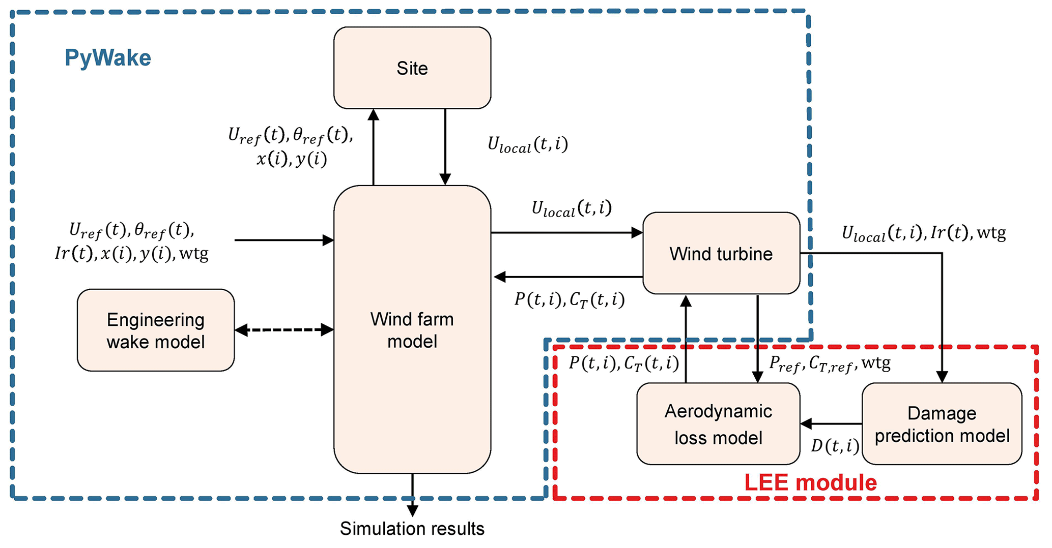
The current section describes the methodology used for modeling the combined aerodynamic effects of LEE in wind farms. The overall workflow of the modeling framework is visualized in Fig. 1. The framework revolves around a central wind farm simulation tool that runs with an engineering wake model and is coupled to a LEE module. The LEE module consists of two sub-modules; first, a damage prediction model is used to provide probabilistic damage estimates based on the site-specific time series of weather inputs and turbine operational data. The damage estimate is then passed on to an aerodynamic predictor which determines the blade-sectional aerodynamic losses. These sectional losses are combined to provide the final output in the form of eroded power and thrust curves. These properties are finally fed back to the central wind farm model and used in the computation of the wake deficits to update the wind farm flow field and turbine power production. The wind farm can be simulated over a time series of wind speed, wind direction, and rain to simulate the gradual development of erosion on each individual turbine in a wind farm. The damage state can be updated at each time step or after a block of time steps to speed up the simulation time. It should also be mentioned that since the modeling framework is modularized, it is very flexible and not limited to the setup used within this paper. The individual models can easily be substituted with other models, provided they take the same inputs and outputs.
2.2 Damage prediction model
The damage prediction model used in this study was originally proposed by Visbech et al. (2023), and the following description will only cover the model in relation to the scope of the present study. For detailed information, the reader is referred to the original paper.
The model is based on an ensemble of 816 small feed-forward neural networks. The networks were trained with mesoscale weather data and blade inspections from seven wind farms located on- and offshore in northern Europe. The mesoscale weather data were provided as hourly time series of wind and precipitation, and the blade inspections were obtained from a combination of manual, ground-based, and drone-based images. The purpose of the damage prediction model is to provide estimates of the erosion damage along the blade, based on time series of turbine local wind speed and rain. Together with turbine-specific operational characteristics, these are used to calculate rain impingement following industry recommendations (DNV, 2020), which is the main predictor variable used by the model. The output from the damage prediction model is an encoded damage value ranging between 0 and 1. The encoded damage from the model is directly related to a specific defect type and severity. The categorization is based on the structural integrity of the blades and therefore represents the urgency of repair actions. Moreover, the encoding scheme allows for continuous and realistic damage progression, similar to that observed from actual blade inspections. Although the categorization scheme is unique to the blade inspections used for training the damage prediction model, it is similar to others proposed in the literature (e.g., Sareen et al., 2014; Gaudern, 2014).
Figure 2 demonstrates the output of the damage prediction model based on a 10-year time series using wind speed and rain as input. The solid line represents the average encoded damage of a wind turbine. Since the model consists of an ensemble of several hundred neural networks, it allows for making probabilistic damage estimates by incorporating uncertainty observed from the blade inspections used during training. This is also visualized in Fig. 2 by the 95 % ensemble confidence interval (CI) predicted by the damage model. Here, we observe the heteroscedastic uncertainty captured by the model, which can be used to introduce realistic damage variability, similar to that observed in the field.
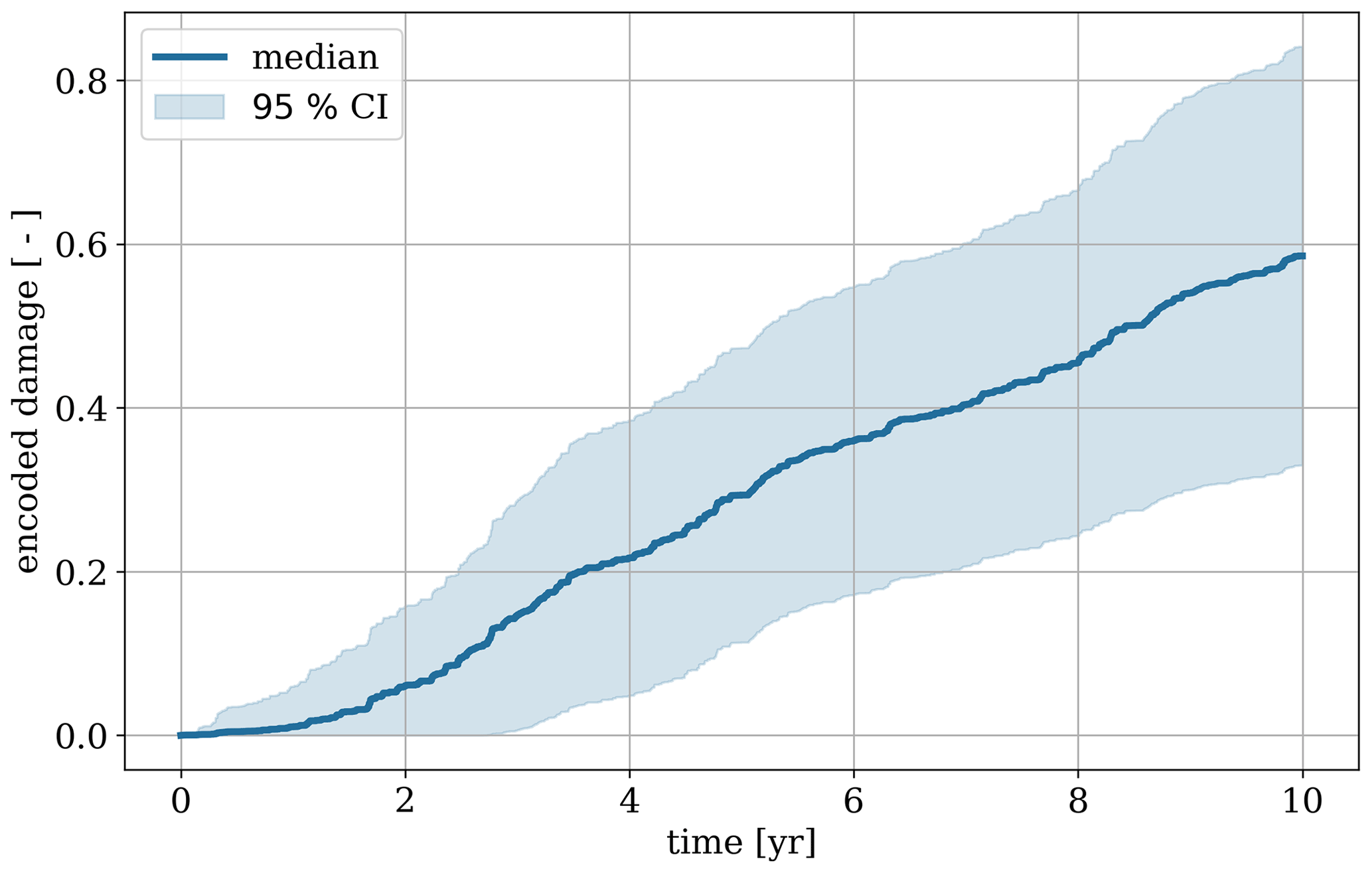
Figure 2Example of the output of the damage prediction model based on 10 years of weather data as input. The graphs show the progression of the encoded damage level from a time series of half-hourly wind speed and rain data. The solid line represents the ensemble median, and the shaded area indicates the 95 % ensemble confidence interval (CI).
2.3 Aerodynamic loss categories
While the damage prediction model provides estimates of the structural erosion damage, it does not consider the associated aerodynamic losses. Doing this requires information on the sectional degradation of the lift-to-drag ratio and maximum lift coefficient due to damages along each blade. It is common to categorize blade inspection data into severity classes by judging the risk of damage progression and potential repair costs, as done for the data underlying the damage prediction model. Yet, severe structural damages, e.g., deep isolated cracks, do not lead to severe aerodynamic losses, whereas structurally insignificant findings, like top coat erosion, do. Therefore an aerodynamic categorization of leading damages needs to be performed independently of the structural assessment.
A standardized aerodynamic loss categorization scheme is yet to be established, as there is insufficient knowledge about the detailed geometric realization of the damages encountered in the field and their corresponding frequency of appearance. For aerodynamic loss assessment, the exact three-dimensional damage topography needs to be known, as even features down to 50 µm can be aerodynamically active. However, with the more frequent appearance of severe damages, a growing number of wind tunnel and numerical investigations have been performed to quantify their aerodynamic impact (Sareen et al., 2014; Gaudern, 2014; Ehrmann et al., 2017; Meyer Forsting et al., 2022a, b, 2023). Applying similar damage topographies resulted in comparable relative changes in the lift-to-drag ratio, despite the use of different airfoils. It is likely that this is also related to having investigated similar Reynolds numbers (≤ 6×10⁶) and thin airfoils (≤21 %) that are usually used in the outer blade region. Aerodynamically, this is rooted in the impact of surface perturbations, also those caused by LEE, being related to the ratio of surface feature height to boundary layer thickness. In turn, this is a function of the Reynolds number, while the airfoil thickness is a proxy for the surface pressure gradient, which again influences the boundary layer. Generally, the biggest drop in performance arises from roughness inducing premature boundary layer transition right at the leading edge, with the aforementioned studies reporting losses between 35 %–50 % with respect to the clean baseline with free transition. With erosion-type damages losses increase by another 10 %–15 %, thus maximally reaching 65 %. As all available loss data were compiled for Reynolds numbers below 6×10⁶, it is difficult to transfer these loss factors directly to modern wind turbines, as their blades can easily operate at 15×106. As the boundary layer transition naturally moves towards the leading edge with increasing Reynolds number, roughness-induced transition has less of an impact at elevated Reynolds numbers. In fact, avoiding premature transition at 15×106 requires a blade surface finish that is hard to achieve in a cost-effective manner even in a factory. To assess the aerodynamic losses at higher Reynolds numbers, two-dimensional CFD computations were performed with EllipSys2D (Sørensen, 1995) for four airfoils with relative thickness below 21 % (NACA 63-418, FFA-W3-211, DU96-W-180, Risø-B1-18, Risø-C2-18) at Reynolds numbers of 5×10⁶, 10×106, and 15×106 and with five levels of leading-edge damage: clean with free transition, clean and fully turbulent, moderate grid-resolved erosion, severe grid-resolved erosion, and severe grid-resolved erosion with a forward-facing step on the suction side (height of located at 0.024c chordwise, with chord length c). The grid-resolved erosion is generated by superimposing multi-directional waves sampled from a spectrum as detailed in Meyer Forsting et al. (2022a). The numerical setup is also identical to the one in Meyer Forsting et al. (2022a) using a structured O mesh with a radius of 45c, first cell height of , and for the clean leading-edge cases 512 cells in the chordwise direction and 256 cells in the wall normal direction. To adequately resolve the erosion, another 256 chordwise cells are added. The k−ω shear stress transport (SST) turbulence closure by Menter (1993) is used, coupled to the eN stability model (Drela and Giles, 1987), and implemented by Michelsen (2002) for the clean transitional case. The freestream turbulence intensity at the airfoil is 0.1 %. The entire workflow from surface grid generation to post-processing was automatized within the Python tool (https://alrf.pages.windenergy.dtu.dk/pye2dpolar/, last access: 29 July 2024), for which details are given in Meyer Forsting et al. (2022a, 2023).
The aerodynamic degradation from leading-edge damage is then computed for each of the five simulated airfoils by determining the drop in the lift-to-drag ratio around the design angle of attack (±2° to account for natural variation) with respect to the clean airfoil performance. The latter is assumed to be represented by a 40:60 blend of the fully turbulent and free transition performance1 (Bak, 2013), as blades are usually designed with a certain safety margin. Similar to the studies mentioned above, the relative drop in the lift-to-drag ratio, as it is defined here, is nearly airfoil independent. In line with structural damage categorization and with the aim to create distinct aerodynamic loss categories, the losses were divided into five categories and labeled with letters to clearly distinguish them from structural classifications. The categories and the associated percentage losses in the lift-to-drag ratio are presented in Fig. 3b for Reynolds numbers of 5×10⁶ and 15×106 (losses for intermediate Reynolds numbers can be linearly interpolated) – covering the operating range of most wind turbines – and approximately capture the behavior found for the different airfoils that were simulated herein and those presented in the literature. This particular categorization is thus only a rough attempt at classifying leading-edge damages aerodynamically and might require future revisions. The first category (a) represents a clean blade, i.e., without any aerodynamic loss. The next two categories (b and c) capture the losses associated with an increasing proportion of pits and gouges covering the leading edge of the blade section in question, which cause early transition. The coverage is about one-third at b and two-thirds at c. Full coverage comes with full erosion of the top coat and corresponds to category d. The final two categories (e and f) are associated with progressive growth in damage depth from the onset of exposure to complete exposure of the laminate. The aerodynamic losses do not grow any further for the types of damages usually observed in the field.
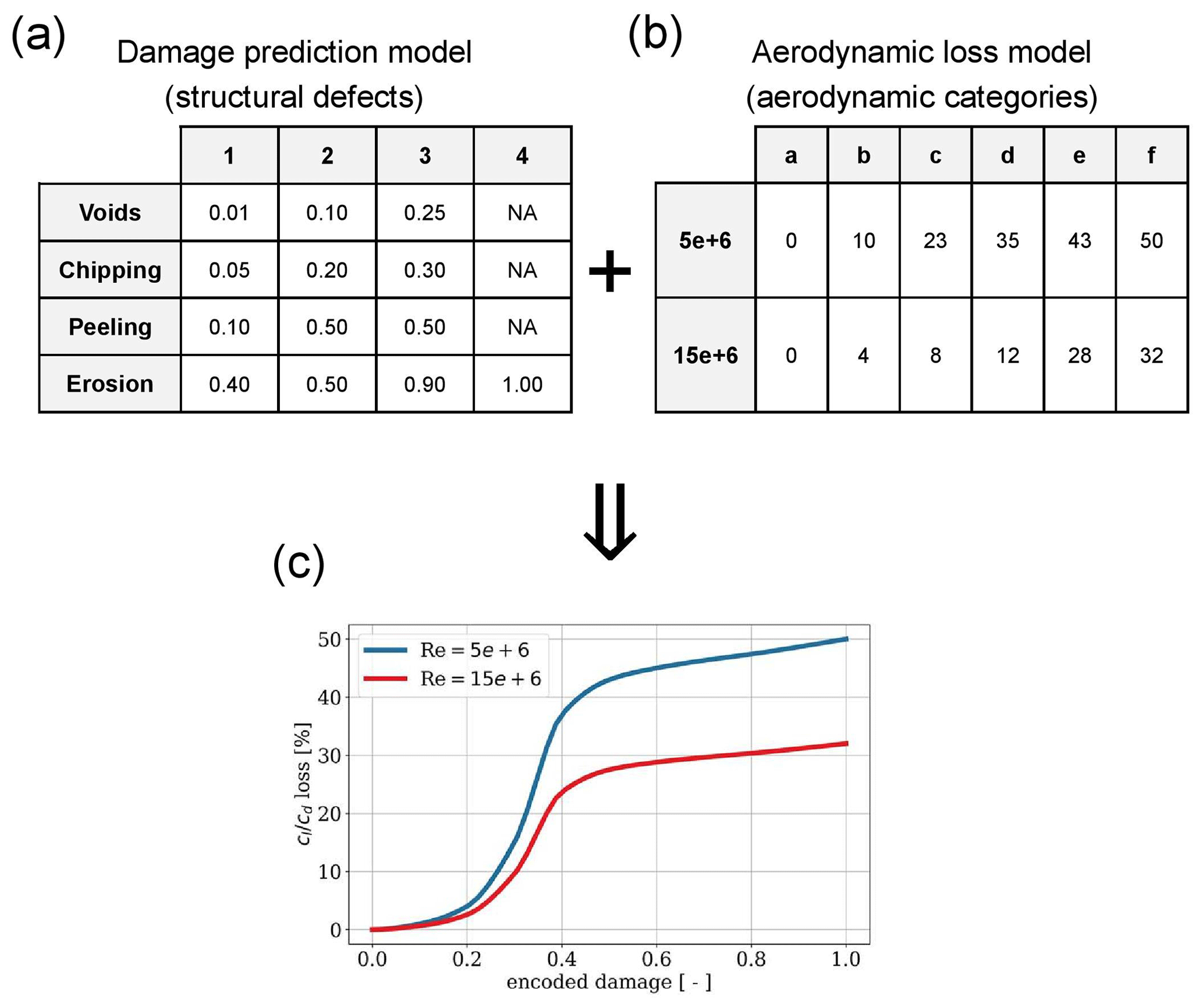
Figure 3Mapping between the damage prediction model and the aerodynamic loss model. Panel (a) shows the structural categories and associated encoded damage level, panel (b) shows the aerodynamic categories and associated percentage lift-to-drag losses, and panel (c) shows final functional coupling between the encoded damage level and aerodynamic loss. Values between the two Reynolds numbers can be interpolated.
2.4 Coupling aerodynamic and structural categories
The original modeling objective of the damage prediction model was to support site-specific repair and maintenance planning. This was done through an encoded damage score representing the damage state of a wind farm in relation to the urgency of repair. As previously mentioned, the purpose of this study is to investigate the aerodynamic effect of LEE for wind farm flow modeling, and for this reason, a relation between structural and aerodynamic defect categorization has to be established.
As mentioned in the previous section, it is difficult to relate aerodynamic categories to structural categories; however here this was attempted by matching the observable damage features. Figure 3a shows the categorization of structural defects (defect type on the vertical axis and defect severity on the horizontal axis) used by the damage prediction model and the corresponding encoded damage value (Visbech et al., 2023). Figure 3b shows the categorization of the aerodynamic losses (Reynolds number on the vertical axis and categories on the horizontal axis), obtained from the CFD simulations and literature review. Figure 3c shows how the two individual schemes are combined to relate the encoded damage and the percentage lift-to-drag ratio. As mentioned before, this was done by matching the observable damage features used for the individual categorizing. It is assumed that aerodynamic losses will grow quickly with the onset of structural damage accumulation as it causes the transition point to rapidly move towards the leading edge. From then on the aerodynamic losses increase more slowly, reaching their maximum once the leading edge is fully eroded.
2.5 Aerodynamic loss model
The main purpose of the aerodynamic loss model is to obtain the loss in annual energy production of a turbine due to leading-edge erosion and to obtain the power and thrust curves of turbines subjected to LEE that can be used by the wind farm simulation tool. In this paper, we use an adaptation of the aerodynamic loss model introduced by Bak (2022a). The tool is a simplified blade-element momentum (BEM) theory model where the blade is divided into annular elements, and the local losses are calculated at each annular element. The model is very light in its implementation as it is independent of the inflow angle, which significantly speeds up the computation. In addition, it includes a simplified tip correction model that only depends on the tip speed ratio (TSR), the blade radius, and the number of blades. The aerodynamic loss model was validated by Bak (2022a) in comparison to a classic BEM model, and it was found that the local power and thrust coefficients along the rotor radius compare well.
The main input parameter to the aerodynamic loss model is the sectional loss in the lift-to-drag ratio, which is provided by the damage prediction model using the structural-to-aerodynamic coupling previously described. Figure 4 illustrates an example of the loss distribution along the blade, where the highest lift-to-drag loss is reached towards the tip, and the erosion severity decreases towards the root. For this representation of the erosion distribution on the blade, it is assumed that the predicted damage occurs at the tip of the blade and that it decreases towards the root, following a cubic relationship. Due to the fact that the most severe damage typically occurs towards the tip of the blade and that the outer part of the blade plays a greater role in aerodynamics, a logarithmic discretization was chosen to divide the blade into sections. Figure 4 provides a visualization of this non-linear discretization.
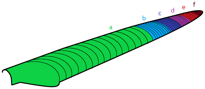
Figure 4Example of a typical distribution of aerodynamic losses along the wind turbine blade. The blade sections are discretized in a non-linear manner, and each section is assigned an erosion severity in terms of lift-to-drag losses (“f” is the most severe erosion, and “a” is the clean case with no loss).
In addition to the loss in the lift-to-drag ratio, there are more inputs that are not always available for a given turbine, such as the design lift coefficient and sectional lift-to-drag coefficient ratios for the clean blade. For those parameters, default values that are obtained from a test turbine are used.
An empirical relation for the thrust coefficient that depends on the tip speed ratio and design lift coefficient is used. The tip loss and lift coefficient ratio of an eroded and clean reference case is included to find the thrust coefficient for the eroded case.
In the aerodynamic loss model, there are no specified control properties. It is assumed that the wind turbine is variable-speed pitch regulated (VSPR) and operates at maximum power coefficient below rated wind speed. If the wind turbine is subject to a constraint on tip speed, which is violated before rated wind speed, a sub-region might occur, where the tip speed ratio is kept suboptimal.
Similarly, it is assumed that the wind turbine is capable of adequately shifting the pitch and rotational speed to adjust for the aerodynamic degradation of the lift and drag coefficients when exposed to erosion. LEE reduces the efficiency of the blade, which effectively shifts the rated wind speed to a higher value. As previously mentioned, these control properties are not specifically defined but are assumed to be inherent to the wind turbine operation.
2.6 Wind farm flow modeling
In order to incorporate the long-term progression of LEE damage into wind farm response modeling, it is important to include the steady-state behavior of wake effects in the simulations. Steady-state engineering wake models offer a significant advantage by enabling the computationally low-cost prediction of wind farm flow fields, including turbine wakes, to assess power capture and ultimately AEP. Compared to more detailed, often dynamic high-fidelity numerical tools such as CFD with much higher computational cost, engineering wake models have been shown to provide comparable accuracy, requiring much lower complexity in their inputs in terms of flow properties and turbine characteristics (e.g., blade geometry, detailed representation of the controller) (Göcmen et al., 2016).
In this study, the steady-state flow within the wind farm is represented using the open-source wind farm simulation tool PyWake (version 2.5) (Pedersen et al., 2023). PyWake provides engineering models for estimating wind farm flow fields, including the Gaussian wake deficit formulation proposed by Bastankhah and Porté-Agel (2014) and presented in Eq. (1) below. PyWake assumes that the wake spreads radially outwards, that the wake deficit follows a Gaussian shape, and that the wake centerline is aligned with the turbine rotor plane. It has shown very good agreement with field observations in several campaigns and wake model benchmarks (e.g., Doubrawa et al., 2020), especially in the far-wake region, and it is utilized in this analysis to estimate the flow characteristics of eroded turbine(s).
Here, is the wake deficit normalized by the freestream velocity; x, y, and z are the streamwise, spanwise, and vertical spatial coordinates; zh is the hub height; D is the turbine diameter; CT is the thrust coefficient of the turbine; and k* is the wake expansion parameter defined by the local turbulence intensity (streamwise) at hub height TIh as (Niayifar and Porté-Agel, 2015)
Additionally, ϵ is proposed as a function of CT (Bastankhah and Porté-Agel, 2014), described by . Therefore, with the expected reduction in CT due to progression of LEE over time, the wake deficit described in Eq. (1) is also anticipated to decrease.
Detailed specifications of the PyWake simulation setup can be found in Appendix A.
The modeling framework described in the previous section is demonstrated through a case study for the Horns Rev 1 offshore wind farm, which is located in the North Sea along the west coast of Denmark. The wind farm was commissioned in 2009 and consists of 80 Vestas V80 2 MW wind turbines, yielding an installed capacity of 160 MW. The layout and geographical location of Horns Rev 1 are shown in Fig. 6, where the minimum spacing between the turbines is 7 rotor diameters (560 m).
Weather data used in the study are obtained from the mesoscale Weather Research and Forecasting (WRF) model used in the New European Wind Atlas (NEWA) (Witha et al., 2019). The data contain wind speed, wind direction, turbulent kinetic energy, and precipitation. The data are provided as time series with a 30 min time resolution and a 3 km grid spacing. Precipitation data are provided at surface level, whereas wind data are provided at 75 m height and extrapolated to hub height using the power law with shear exponent α=0.1.
The wind climate at Horns Rev 1 is governed by westerlies coming from the sea, thereby providing a very good wind resource. The mean wind speed at hub height (70 m) is 9.3 m s−1, and the mean wind direction is 252°. The average turbulence intensity (TI) is 6.7 %. Figure 5 illustrates the statistical weather conditions at the site shown by a wind rose on the left and the exceedance probability of rain on the right. The annual rainfall was found to be 1053 mm yr−1, with a large proportion falling in autumn. The rain exceedance probability also shows that rain occurs around 6 % of the time. A lower-bound threshold of 0.5 mm h−1 is applied to the rain to account for the mesoscale model uncertainty, which is also observed from the sharp edge on the graph at this value.
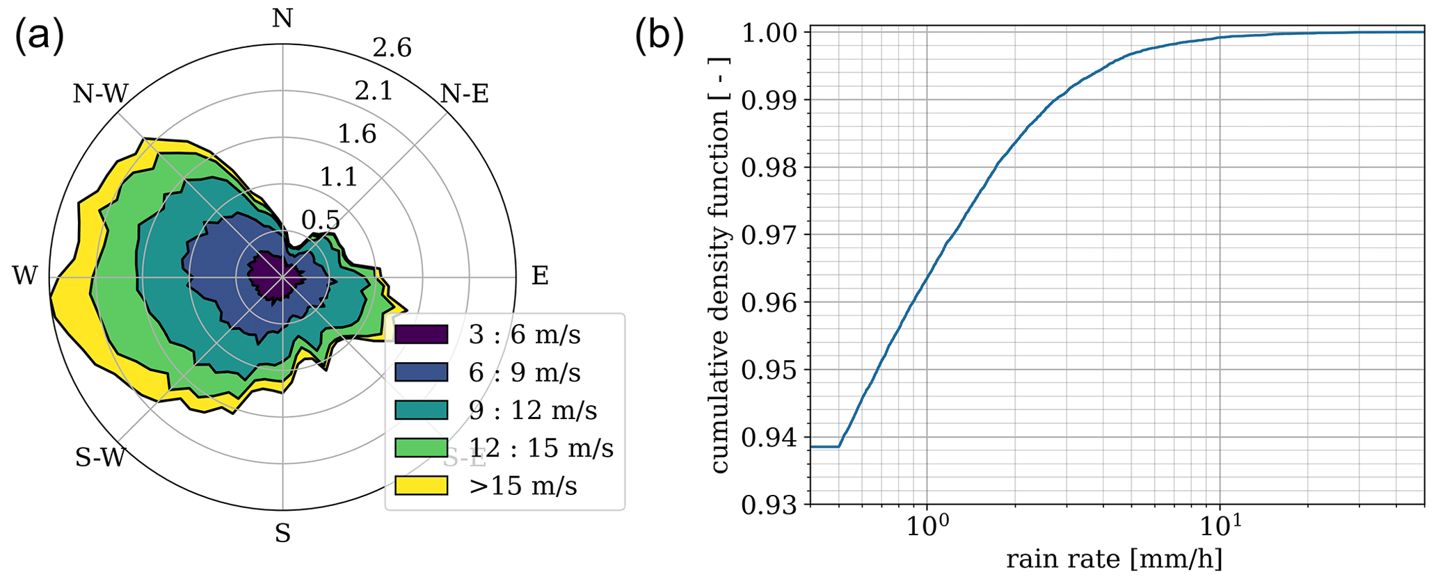
Figure 5Weather conditions at Horns Rev 1 given by (a) a wind rose with a mean speed of 9.3 m s−1 and a mean wind direction of 252° and (b) the cumulative density function of rain with a mean annual rainfall of 1053 mm yr−1. A lower-bound threshold of 0.5 mm h−1 is applied to the rain data.
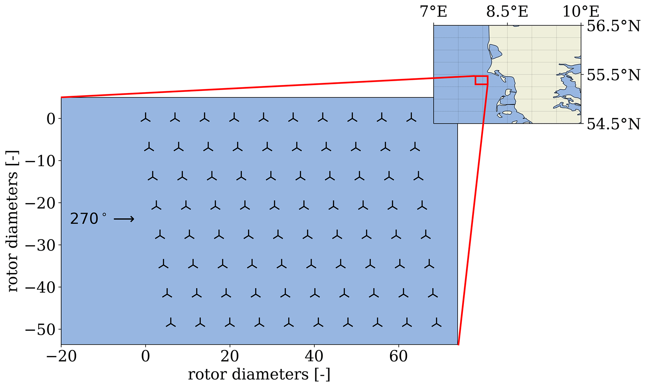
Figure 6Layout and geographical location of the Horns Rev 1 wind farm. The minimum spacing between the turbines is 7 rotor diameters.
4.1 Deterministic simulations
The first step in the analysis is to compare the effect of eroded blades when modeling a single turbine with a full wind farm. To do this, we run two simulations, one using a single Vestas V80 turbine and one using the full Horns Rev 1 wind farm. For both simulations, 10 years of weather data and wind turbine specifications from Horns Rev 1 are used for simulating the operation of the wind turbines and their gradual aerodynamic degradation caused by LEE. A constant Reynolds number of 5×10⁶ was used for the entire blade, which is based on the limited airfoil information on the Vestas V80 2 MW wind turbine and the typical distribution of Reynolds numbers for wind turbines of a similar size (Ge et al., 2016). For these simulations, only the ensemble mean from the damage prediction model is used as an output for updating the damage state of all the turbines, thereby providing a deterministic damage estimate only. In this case, the only damage variability comes from the local wind speed observed by each turbine. To account for randomness in the weather data, the 10-year simulations are run for 10 random seeds.
Figure 7 shows the estimated AEP loss of the eroded turbine and wind farm relative to its identical but non-eroded counterpart. This allows for a fair comparison of the AEP loss even though there is a difference in the absolute per-turbine AEP between the single turbine and the wind farm due to wake losses. The blue bars indicate the relative AEP loss for the single turbine, and the red bars show the relative AEP loss for the full wind farm. For both cases, the mean AEP loss over the full simulation is listed in the legend. Based on 10 years of operation, we observe a difference in AEP loss between simulating a single wind turbine compared to an entire wind farm. Generally, the trends from the single turbine and the wind farm are very similar. The AEP loss is observed to be relatively small for the first 3–4 years but quickly increases after this point. We also observe that the first 5 years of operation account for less than 15 % of the total loss for both cases. As shown, the main difference between the two cases is the magnitude of the power loss. For both cases, the highest AEP loss is observed to occur in the last 2 years of the simulation with a maximum AEP loss of 2.9 % for the single turbine and 2.7 % for the wind farm. This corresponds to a 7 % reduction with respect to simulating the single wind turbines versus the full wind farm. The average AEP loss for the entire simulation period was 1.5 % for the single turbine and 1.4 % for the wind farm.
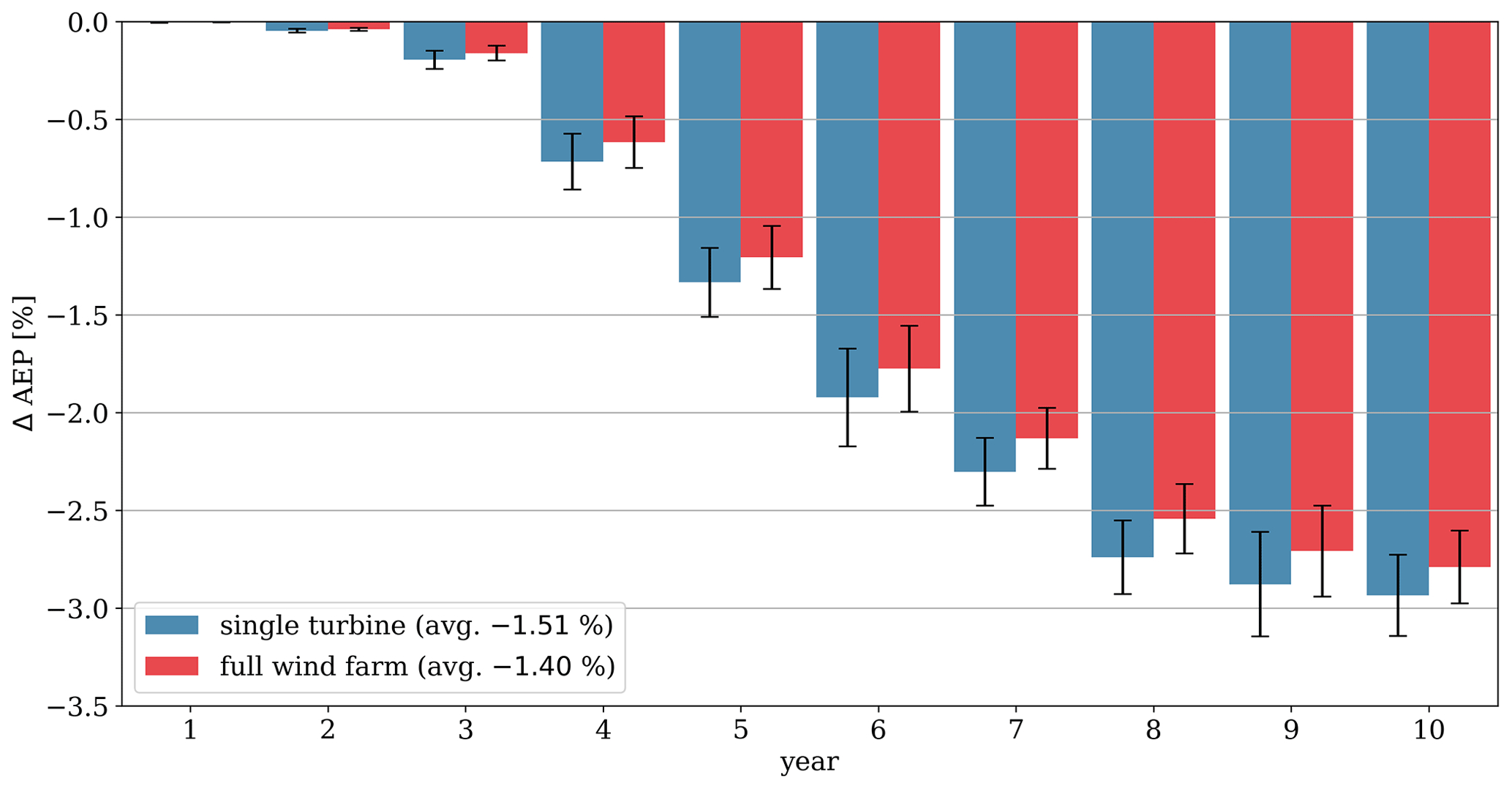
Figure 7Comparison of relative AEP change for a single turbine vs. the full wind farm. In both cases, the AEP is calculated relative to the non-eroded counterpart. The graphs show the simulation over a period of 10 years using 10 seeds to compute the mean and standard deviations.
Since the simulations are run for a period of 10 years, it is possible to assess the aerodynamic condition of the blade at certain points throughout the simulation. Figure 8 shows snapshots of the average wind farm lift-over-drag loss along the normalized blade after year 1, 3, 5, and 10. In all cases, the maximum loss is assumed to occur at the tip of the blade from where it decreases towards the root. It is also observed that the aerodynamic loss only affects the blade to a certain extent. We observe that the distribution of aerodynamic loss does not change linearly along the blade and also not linearly over time.
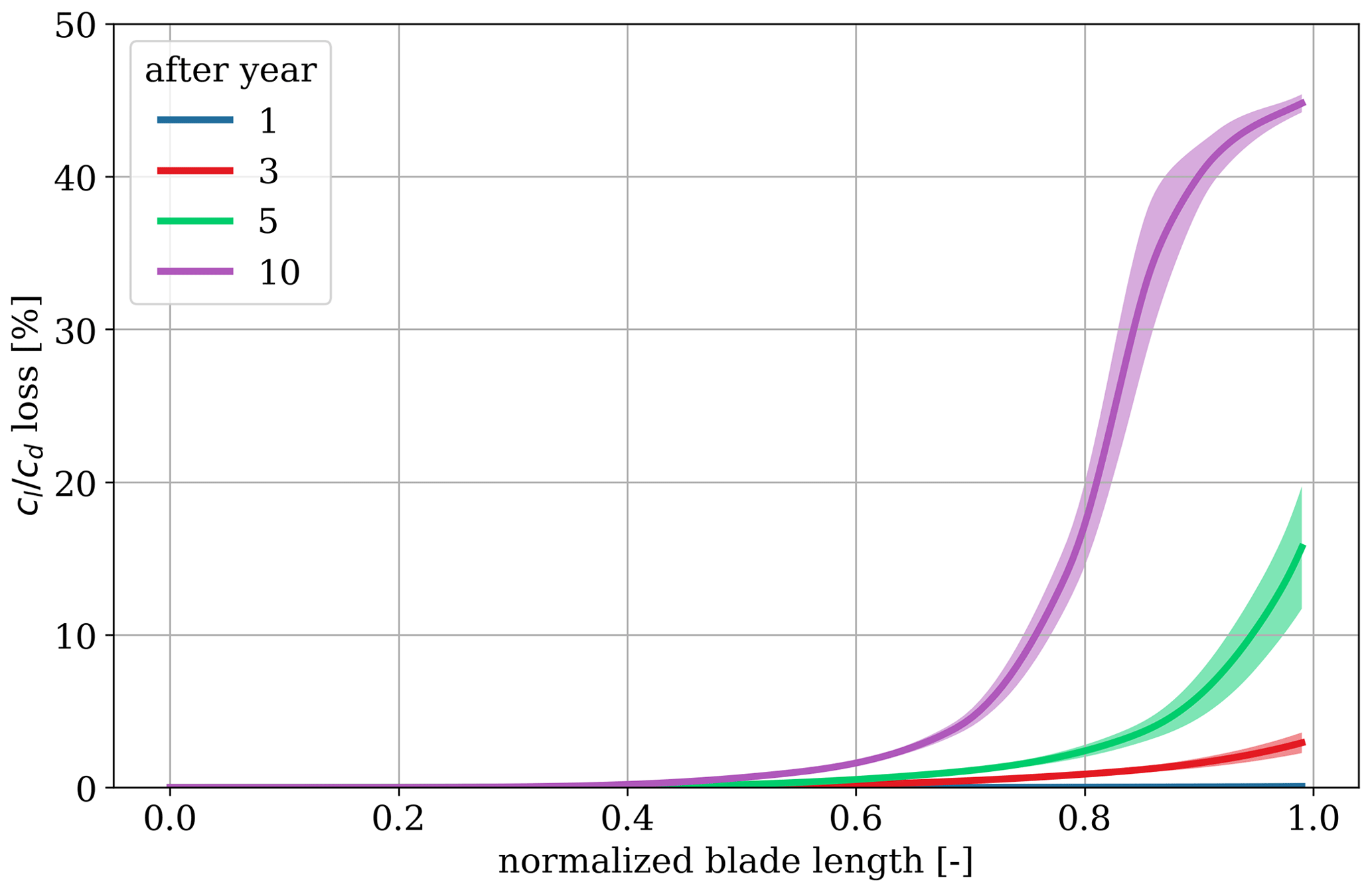
Figure 8Snapshots of the average wind farm lift-over-drag losses along the blade after 1 year, 3 years, 5 years, and 10 years of operation.
After year 1, the erosion damage is very small and barely causes any aerodynamic losses. After year 3, the maximum loss at the tip is around 3 % and decreases smoothly inwards. This appearance resembles a slightly roughened surface on the outer 20 % of the blade, which causes insignificant AEP losses. After year 5, we observe a significant increase in maximum aerodynamic loss. At the tip, the loss is on average around 15 % but decreases rapidly towards the root. This appearance resembles the initiation of more severe erosion locally at the tip. Here, the aerodynamic loss is observed to decrease much faster when moving towards the root. After year 10, the maximum loss reaches around 45 %, which is close to the obtainable maximum. We also observe that a larger extent of the outer blade is expected to experience significant aerodynamic loss. This represents the start of stagnation of the erosion at the tip in terms of aerodynamic loss. The aerodynamic loss is not expected to increase much anymore, but the damage progression will occur in the form of a much larger damage extent. We also observe that a larger extent of the blade is affected by a roughened surface.
It should be mentioned that the damage prediction model is limited by the range of the outputted encoded damage (ranges between 0 and 1). This also limits the aerodynamic loss since the two models are directly coupled. In real-life conditions, it is expected that damages beyond this range could occur if the blade is left fully untreated. However, it is also expected that blades are typically inspected annually and repaired accordingly, i.e., before extreme damage occurs. Thus, as mentioned previously, the damage encoding scheme used by the damage prediction model is based on the range of allowable defects observed from real blade inspections.
As stated earlier, the aerodynamic properties governing the wind farm simulation are the power and thrust curves. The thrust coefficient governs the wake behavior in the engineering wake model, and the power curve directly affects the energy production. Since we make an explicit distinction between these two properties, we are able to directly separate the contributions from each of them. This is done by running two parallel simulations where the power and thrust coefficient curves are degraded independently; i.e., the power curve is eroded, and the thrust coefficient is assumed to be clean and vice versa. This allows us to exactly quantify which contribution comes from which of the two properties.
Figure 9 visualizes the relative AEP loss from the isolated aerodynamic performance properties over the full simulation period of 10 years. As expected, the isolated effect on the power curve is observed to cause a negative effect on the overall AEP. It is also observed that the isolated contribution from the eroded power curve corresponds very closely to the relative AEP loss observed for the single-turbine case in Fig. 7. This indicates that erosion-induced power curve degradation does not vary significantly, and the main variation comes from the reduced local wind speed caused by wakes. Oppositely, the isolated effect from the eroded thrust coefficient is observed to positively contribute towards AEP. At first, it might seem counterintuitive that erosion can actually contribute to a power gain. However, we assume that erosion reduces the aerodynamic efficiency, which also reduces the thrust force that the rotor exerts on the wind, thereby diminishing the wake deficit and leaving more energy for downstream turbines. The contribution is solely relevant for wind farms where wake losses are present. Combining the individual contributions from the power and thrust coefficients, we end up with an overall loss, corresponding exactly to the relative power change observed in Fig. 7.
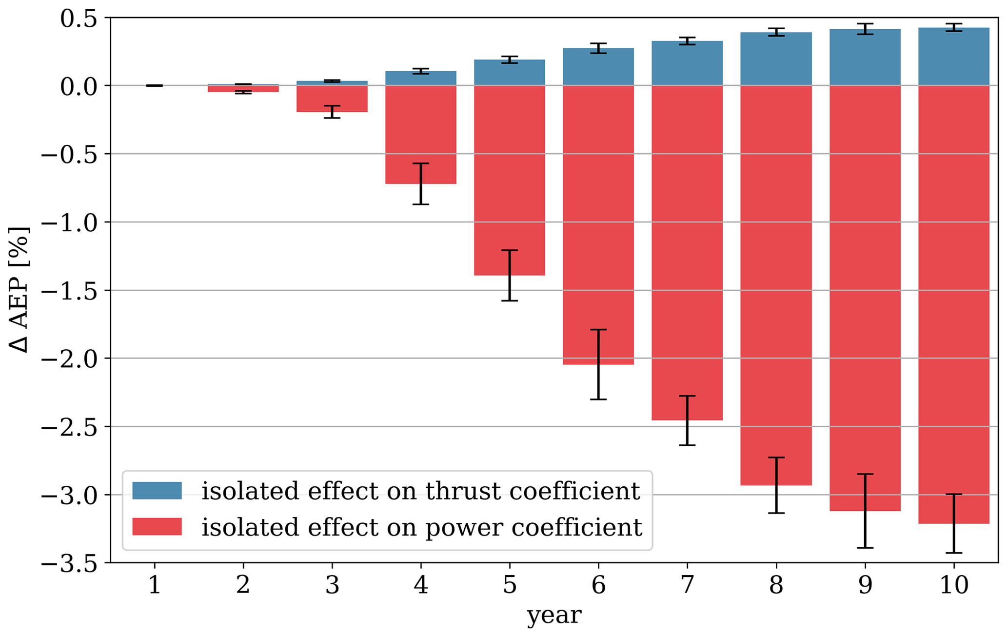
Figure 9Relative AEP changes from isolated aerodynamic rotor properties. The red bars indicate the isolated contribution coming from the power coefficient, and the blue bars indicate the isolated contribution coming from the thrust coefficient.
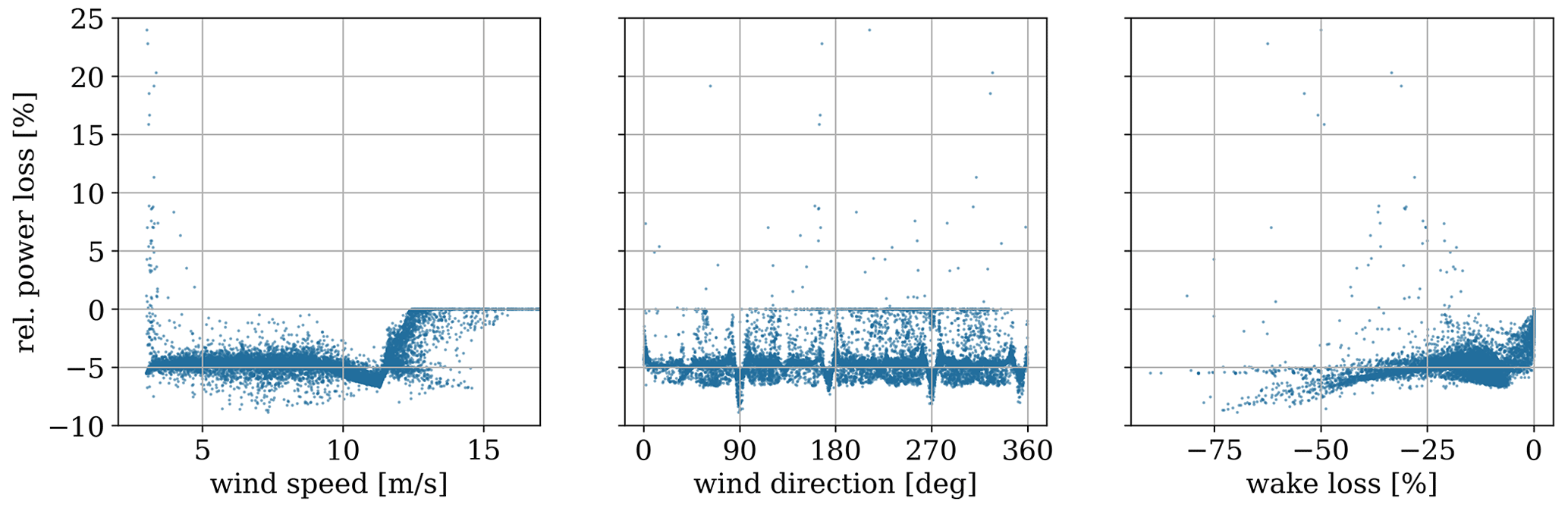
Figure 10Correlation plot showing the relation between the power loss and freestream wind speed, wind direction, and reference wake loss.
Until now, we have focused on AEP, which provides key information in a simple manner. Since the simulations are based on half-hourly data, we can also analyze the results directly at this temporal frequency. Figure 10 shows the pairwise relationships between half-hourly variables from the full wind farm simulation. The row of sub-figures shows the relative power loss plotted against three other variables, namely the wind speed (left), wind direction (middle), and wake loss (right). The plots are based on data only from the last year (year 10), where the effects from LEE are most apparent. Firstly, we identify that the majority of the simulated hours results in power losses of up to 7 % and that these occur mostly in the operational region below rated. For wind speeds below 10 m s−1, the relative power loss is centered around −5 %, though with a lot of scatter. The loss diminishes for wind speeds above rated where the effect of LEE is also expected to be absent. Several observations have a high erosion-induced power gain of up to 25 %. However, looking at the relation between relative power and wind speed, we note that these instances only occur at low wind speeds (below 5 m s−1), thereby having a limited impact on the overall power loss. During these unique hours, the effects from reduced wake deficits overtake the effects from the degraded power curve, leading to an overall power gain. Wake losses are heavily dependent on wind direction, and it is expected that erosion-induced wake loss mitigation is also wind direction dependent. This is apparent when looking at the relation between power loss and wind direction. Certain periodic wind directions cause a consistently smaller or higher relative power loss than others. These wind directions correspond exactly with the physical alignment of the turbine rows, i.e., along the rows of the wind farm layout. The relation between power loss and wake loss supports the fact that the highest relative power loss occurs for highly waked instances. Finally, it should be mentioned that we only considered the relative power loss. It was found that 95 % of the absolute power loss occurred in the wind speed region between 8–14 m s−1.
4.2 Probabilistic simulations
Previous simulations have been performed using the ensemble mean as the sole deterministic output from the damage prediction model. In this case, the only damage variation across the wind farm comes from the wake-induced changes in effective wind speed observed by each wind turbine. This variation effectively changes the operational rotor speed of the individual turbines, but the maximum percentage difference for the aerodynamic losses across the wind farm was found to be less than 1 %.
The ensemble capabilities of the damage prediction model also allow for making probabilistic damage estimates, thereby introducing the uncertainty captured by the damage model. Initially, we use the ensemble inverse cumulative density function (CDF) to provide a probabilistic damage output. Figure 11 shows the probabilistic simulation results for the full wind farm using the same 10 years of weather data as inputs. The figure on the left shows the 95 % confidence interval of the relative AEP loss with the 50th percentile (median) indicated by the solid line. The figure on the right shows the CDF of the encoded damage at years 1, 3, 5, and 10.
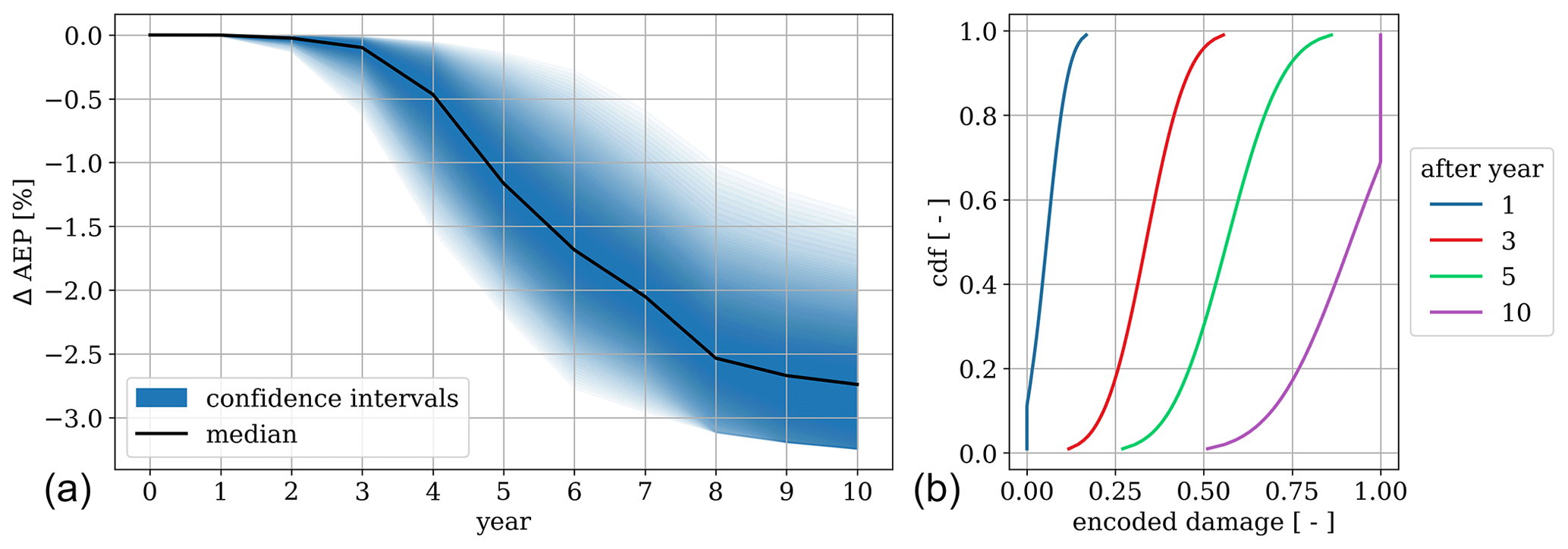
Figure 11(a) Confidence intervals of the relative wind farm AEP loss with the median indicated by the black line and (b) the cumulative density functions of the encoded damage after years 1, 3, 5, and 10.
From the relative AEP loss, we observe the uncertainty being propagated from the damage prediction model. The model uncertainty is very low for the first years but rapidly increases after year 2. At the 10th year, we expect the relative AEP loss to range between 1.4 %–3.2 % based on the 95 % CI. We observe a slightly asymmetric model uncertainty with higher-confidence weight towards the upper quantiles, indicated by the CI bands being slightly more narrow. It is especially visible for the last couple of years where the upper quantiles reach the upper limit of the encoded damage, i.e., a value of 1. This is also more clearly visible from the cumulative density function, which shows a large proportion of probability being constrained at year 10. Finally, we observe the feature of the incubation period, which is also captured by the damage prediction model. This is observed as the very-limited erosion impact during the first few years of operation.
In addition to directly outputting a specific damage percentile for all wind turbines, the damage across the wind farm can be randomly sampled using the inverse cumulative density function, i.e., using Monte Carlo (MC) sampling. This would better represent the stochastic damage distribution observed from field inspections. Based on 250 random MC simulations, the AEP variability was found to increase over time, but the maximum percentage difference (between the most/least productive) after 10 years was found to be less than 0.2 %. Of course, this should be seen in light of the total energy production of the entire wind farm, and the corresponding revenue might end up being considerable. Because we simulated the full wind farm for each random instance, the aggregated energy production of the 80 wind turbines ensures convergence of the summary statistics, which is why the variability is so low. If the same experiment was performed for individual wind turbines or a much smaller wind farm, the variability would be expected to be correspondingly larger.
Finally, the random sampling provides an indication of the modeling sensitivity, which could potentially be used to better prioritize repairs. For each MC simulation, we assume that one turbine is fully repaired after year 9; i.e., its aerodynamic properties are reset to a clean state. We iterate through every turbine in the wind farm and evaluate the relative impact on the AEP for the remaining year, i.e. year 10. This procedure is performed for all MC simulations and allows for prioritizing the order in which each turbine should be repaired to obtain the largest gain in AEP. For each MC simulation we get 80 samples, one for each wind turbine repair, which can be used to assess the effect from that individual turbine. Due to computational costs, a simpler wake model was used where only the steady wake deficits are considered; i.e., no turbulence model is included. The results are analyzed quantitatively by ranking them according to their individual AEP gain. The results are summarized in Fig. 12, which shows, on the left side, the direct relation between the AEP gain and the damage level of the repaired turbine. Each point represents a repaired turbine, and the total number of points is therefore . In addition to showing the relation between AEP gain and damage level, the points are also colored according to their reference AEP contribution, which is shown in the plot on the right (normalized between 0 and 1). Here, we show the mean AEP contribution from each of the turbines in the wind farm based on the 250 MC simulations. Unsurprisingly, the inner turbines are expected to contribute less since they will be operating more frequently in the wake deficit of the outer turbines. The biggest contributor is the turbine located in the southwestern corner, which contributes almost 9 % more than the smallest contributor.
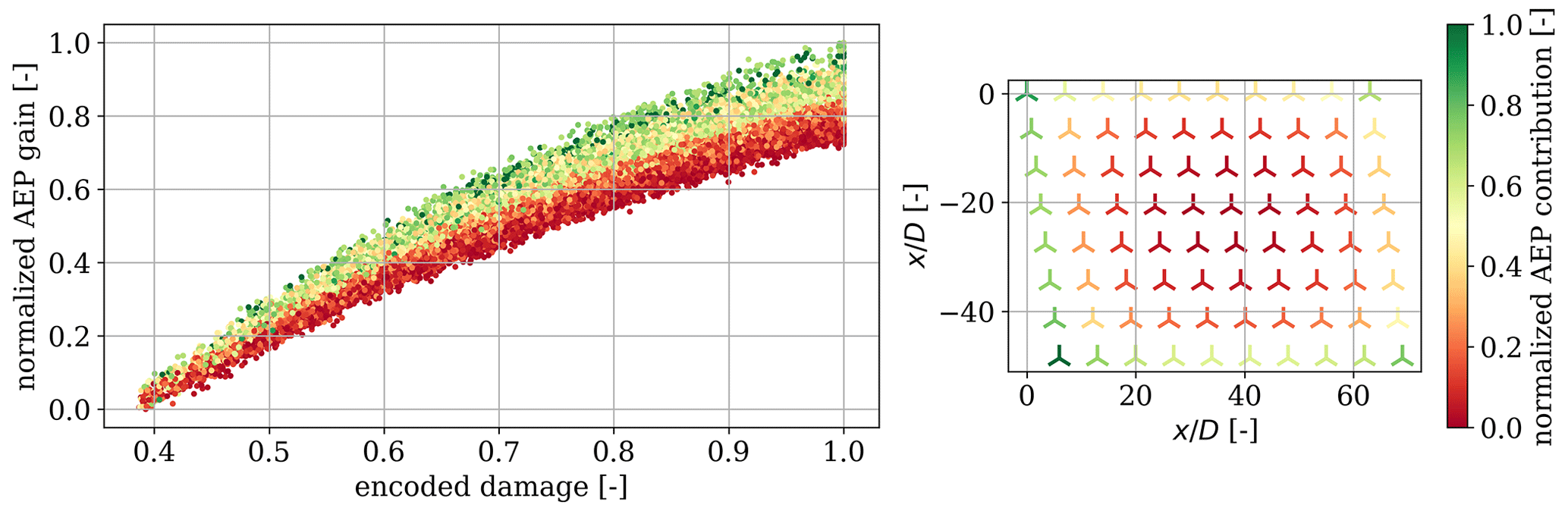
Figure 12AEP gain plotted against the damage level of the repaired turbine. The colors indicate the reference AEP contribution, which is also shown in the figure on the right. Both the AEP gain and the reference AEP have been linearly normalized.
It can be seen that there is a very strong correlation between the encoded erosion damage and the added energy production. This verifies that, generally, the overall biggest gain in energy production is obtained by repairing the most damaged turbine. This also corresponds with previous findings showing that the largest contribution to the power loss comes from the eroded power curve. Secondly, we also observe a correlation between the reference AEP contribution and the added energy production. This indicates that in a case with two equally damaged wind turbines, the turbine providing the highest contribution relative to the overall energy production should be prioritized over smaller contributors. This favors the turbines positioned in the outer rows of the wind farm and especially on the side of the prevailing wind direction. We even observe several instances where it is more favorable to repair less damaged turbines, since their relative AEP contribution is larger. Potentially, a third priority could be repairing the turbines that cause the biggest reduction in wake loss. As previously shown, LEE reduces wake deficits, which in turn contributes positively to the overall energy production. A very weak correlation was found between wake reduction and added energy production. This indicates that an energy production gain can be achieved by prioritizing turbines that contribute the least to wake reduction. It is difficult to conclude if the correlation implies a causal relationship, and the prioritization would only be relevant in extremely rare instances.
The simulation of LEE is challenging considering its multidisciplinary nature, which involves several fields of science and engineering, such as aerodynamics, materials science, mechanical engineering, meteorology, etc. In the present study, we coupled a damage prediction model with an aerodynamic loss model to simulate the progression and aerodynamic effect of LEE in wind farms. Many underlying assumptions affect the results of the present study, and we try to justify, evaluate, and discuss these in the following section.
Wind farm flow modeling on its own is a very complex discipline. We typically distinguish between steady-state and dynamic modeling, and in the present study, we employed a steady-state Gaussian wake deficit model for estimating wake losses across the wind farm. The main assumption is the constant wind flow across the wind farm where the steady flow is assumed to be valid for the entire time bin. Since it assumes a constant wind flow, steady-state flow modeling cannot capture the effects of turbulence and other dynamic flow phenomena that occur in the atmosphere. For example, it cannot account for any transient effects, such as sudden changes in wind speed or direction, changes in atmospheric stability, and other meteorological phenomena.
On the other hand, dynamic wind farm flow modeling is a more advanced technique that takes the dynamic nature of the wind flow into account. It considers changes in wind speed, wind direction, and turbulence at a much higher temporal resolution. The simulation includes detailed information about wind turbine interactions and the surrounding atmosphere. Dynamic modeling is more complex and computationally expensive compared to steady-state modeling, but it does provide more accurate and detailed information about wind farm performance. In addition, dynamic wind farm flow modeling requires a much more detailed and accurate representation of wind turbines and the surrounding environment, which can be challenging to obtain.
The scope of the present study was to demonstrate the aerodynamic effects of LEE in wind farms through a combination of erosion, aerodynamic, and wake modeling. Since the requirements for dynamically modeling all of these properties over long time periods were unfeasible, the simulations were performed using steady-state wind farm flow modeling. This type of modeling fidelity is commonly used for a long-term simulation of wind farms where the low-order statistical moments are of interest. However, a future study investigating high-fidelity flow modeling of eroded wind turbines is required to accurately assess the dynamics as well. Such an analysis could be carried out for specific atmospheric and meteorological conditions at well-predefined erosion levels to limit the computational requirements. It could similarly be used with higher-fidelity wind turbine.
One of the main uncertainties related to erosion modeling is the assumed relationship between the output of the damage prediction model, which is used as input for the aerodynamic loss model. As previously described, it is very difficult to convert between structural and aerodynamic defects as they are not weighted equally. Current repair recommendations are primarily based on structural integrity, but there might be a potential financial benefit from also considering the aerodynamic impact. The conversion table from Fig. 3 provides the relationship used for the study and is based on results from a collection of literature and CFD simulations. However, it could be of interest to propose an additional uncertainty parameter to this currently deterministic relationship. This would allow for mimicking the uncertainty-related defect categorization from blade inspections.
In the present study, the output from the damage prediction model was always assumed to be located at the tip and to decrease with a cubic relation towards the root. It was shown by Visbech et al. (2023) that the average distribution of defects from more than 550 blade inspections followed a similar profile. For this reason, we argue that the statistical distribution is more realistically represented by a continuous function rather than by a step function as is usually suggested in the literature (Gaudern, 2014; Sareen et al., 2014; Maniaci et al., 2020). However, blade inspections and laboratory testing of newer coating materials show that erosion defects tend to be more randomly distributed along the blade and do not always initiate at the tip. Therefore, it could be of interest to implement a stochastic defect distribution, which would better resemble this behavior.
One of the key challenges related to modeling aerodynamic loss from LEE is validating the results. Several assumptions were made for the aerodynamic loss model used in the present study in order to make the modeling process more tractable. These assumptions can introduce uncertainties, particularly if the assumptions are not well validated or do not accurately reflect real-world conditions. Validating the aerodynamic degradation of power curves is incredibly difficult using operational data such as those obtained from the SCADA system. For this reason, the main type of validation will still have to come from high-fidelity aeroelastic simulation tools. The aerodynamic effect of LEE has only recently been quantified using operational field data (Panthi and Iungo, 2023).
LEE is expected to have an even larger impact on wind turbines in the future (Pryor et al., 2021; Shields et al., 2021). Generally, we observe new turbines to have longer blades and operate at higher tip speeds, which effectively increases the rate at which erosion initiates and develops. At the same time, new leading-edge protection (LEP) systems are being developed to better withstand more severe operational conditions. These effects contravene and complicate the generalizability of LEE modeling in the future.
We also expect wind farms to become larger in size, which would change the wind farm flow field. In the present study, the effect on the power curve would not be expected to change considerably since the damage prediction model is not very sensitive to changes in tip speed (which is why we also see very little inter-turbine damage variability for the wind farm). However, the effects from an eroded thrust coefficient would scale non-linearly with wake loss. Therefore, the potential wake reduction is dependent on the layout.
Site-specific weather conditions might also influence the results presented in this study. Less windy sites would result in a longer incubation period, but since LEE only affects the aerodynamic properties below rated, it would lead to a relatively larger power loss. Other sites might have a strong correlation between rain and wind direction (e.g., close to a mountain ridge), which would lead to more damage variation across the wind farm. Adding uncertainty properties to the weather inputs (wind speed, wind direction, and rain) could allow for better addressing the sensitivity to these parameters.
LEE has started to be regarded as a potential operation and maintenance improvement in wind farm control (Meyers et al., 2022), e.g., through erosion-safe operation as demonstrated by Bech et al. (2018). With this mitigating strategy, the rain impinging on the blade is reduced through rotor speed reductions during episodes of heavy rain. The damage is thereby reduced at the cost of energy production. However, erosion-safe operation has not been demonstrated in real life, nor has it been implemented within wind farm flow control. Implementing erosion-safe operation in farm control strategies would require the modeling of wake impacts between the turbines and estimating the AEP loss due to eroded blades in the wind farm. To work towards a wind farm flow control algorithm that includes erosion-safe operation, we first need a modeling framework that can predict damage progression and AEP loss within a wind farm.
Finally, it can be mentioned that the modeling framework presented in this paper could potentially be coupled with real blade inspections following a Bayesian updating scheme approach (Asgarpour and Sørensen, 2018). The blade inspections would provide true damage distributions for all blades, thereby diminishing the model uncertainty at the time of inspection. The damage prediction model could be calibrated to match the observed damage distribution, and the associated past AEP loss would then be obtained through propagating back in time. Having calibrated the damage prediction model, it could be used to estimate expected AEP loss for a given period assuming no repair, which would allow for much more informed decision-making.
LEE affects the aerodynamic properties of a wind turbine and thereby reduces rotor performance. This directly decreases the energy production, but it potentially also reduces the overall wake losses, which is not considered when modeling LEE on individual turbines.
In this study, we used a modeling framework that combines damage prediction and aerodynamic loss modeling with steady-state wind farm flow modeling. The framework can be used to efficiently simulate the long-term aerodynamic effects of LEE using site-specific mesoscale weather data and basic wind farm specifications.
The modeling framework was used to simulate the development of LEE on an offshore wind farm over a simulation period of 10 years. Comparing the wind farm simulation to that of a single wind turbine, it was found that AEP losses were overestimated with up to 7 % when neglecting the effect on wake reduction. The average AEP loss for the wind farm was found to be 1.4 %, with a maximum AEP loss of 2.7 % occurring in the last year.
A Monte Carlo-based sensitivity analysis was carried out to establish a probabilistic priority list of turbines which should be repaired first to maximize energy production. It was found that the level of erosion damage was generally the governing factor, but specific turbines which contribute relatively more to the overall energy production should be prioritized in certain cases to maximize energy production.
The main limitations of the study are related to the coupling between structural and aerodynamic damages and verification of the aerodynamic losses through simulations with higher fidelity. Future work should emphasize uncertainty quantification through probabilistic modeling, which could be coupled to real inspection data through a Bayesian updating scheme.
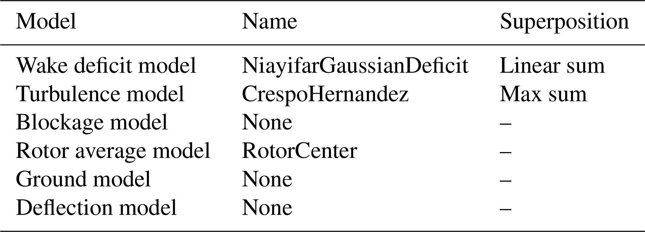
Table A1List of the engineering models used in the PyWake simulation setup.
Software code and data developed and used for this study can be made available by the corresponding author (Jens Visbech) upon request.
JV led the writing of the paper and software development. TG mainly contributed to the damage prediction and wind farm flow modeling. PER mainly contributed to the wind farm flow modeling and PyWake implementation. ÖSÖ and AMF mainly contributed to the aerodynamic loss model. AMF devised the aerodynamic loss categories and conversion scheme. ÁH mainly contributed to the design of the overall project. All authors contributed to the writing and editing of the paper.
The contact author has declared that none of the authors has any competing interests.
Publisher’s note: Copernicus Publications remains neutral with regard to jurisdictional claims made in the text, published maps, institutional affiliations, or any other geographical representation in this paper. While Copernicus Publications makes every effort to include appropriate place names, the final responsibility lies with the authors.
The authors would like to acknowledge everyone at DTU Wind and Energy Systems who was involved in the LEE Cross-Cutting Activity (CCA), which was carried out in 2022.
This paper was edited by Emmanuel Branlard and reviewed by two anonymous referees.
Asgarpour, M. and Sørensen, J. D.: Bayesian Based Diagnostic Model for Condition Based Maintenance of Offshore Wind Farms, Energies, 11, 300, https://doi.org/10.3390/en11020300, 2018. a
Bak, C.: Aerodynamic design of wind turbine rotors, in: Advances in Wind Turbine Blade Design and Materials, Elsevier, 59–108, ISBN 978-0-85709-426-1, https://doi.org/10.1533/9780857097286.1.59, 2013. a
Bak, C.: A simple model to predict the energy loss due to leading edge roughness, J. Phys. Conf. Ser., 2265, 032038, https://doi.org/10.1088/1742-6596/2265/3/032038, 2022a. a, b, c
Bak, C.: Airfoil Design, in: Handbook of Wind Energy Aerodynamics, edited by: Stoevesandt, B., Schepers, G., Fuglsang, P., and Yuping, S., Springer, 95–122, ISBN 978-3-030-31306-7, https://doi.org/10.1007/978-3-030-31307-4_3, 2022b. a
Bak, C., Fuglsang, P., Johansen, J., and Antoniou, I.: Wind tunnel tests of the NACA 63-415 and a modified NACA 63-415 airfoil, no. 1193(EN) in Denmark, Forskningscenter Risoe, Risoe-R, ISBN 87-550-2716-4, 2000. a
Bastankhah, M. and Porté-Agel, F.: A new analytical model for wind-turbine wakes, Renew. Energ., 70, 116–123, https://doi.org/10.1016/j.renene.2014.01.002, 2014. a, b, c
Bech, J. I., Hasager, C. B., and Bak, C.: Extending the life of wind turbine blade leading edges by reducing the tip speed during extreme precipitation events, Wind Energ. Sci., 3, 729–748, https://doi.org/10.5194/wes-3-729-2018, 2018. a, b
Cappugi, L., Castorrini, A., Bonfiglioli, A., Minisci, E., and Campobasso, M. S.: Machine learning-enabled prediction of wind turbine energy yield losses due to general blade leading edge erosion, Energ. Convers. Manage., 245, 114567, https://doi.org/10.1016/j.enconman.2021.114567, 2021. a
Castorrini, A., Cappugi, L., Bonfiglioli, A., and Campobasso, M.: Assessing wind turbine energy losses due to blade leading edge erosion cavities with parametric CAD and 3D CFD, J. Phys. Conf. Ser., 1618, 052015, https://doi.org/10.1088/1742-6596/1618/5/052015, 2020. a
Castorrini, A., Venturini, P., Corsini, A., and Rispoli, F.: Machine learnt prediction method for rain erosion damage on wind turbine blades, Wind Energy, 24, 917–934, https://doi.org/10.1002/we.2609, 2021. a
DNV: RP-0573, Evaluation of erosion and delamination for leading edge protection systems of rotor blades, https://tinyurl.com/DNV-RP0573 (last access: 29 July 2024), 2020. a
Doubrawa, P., Quon, E. W., Martinez-Tossas, L. A., Shaler, K., Debnath, M., Hamilton, N., Herges, T. G., Maniaci, D., Kelley, C. L., Hsieh, A. S., Blaylock, M. L., van der Laan, P., Andersen, S. J., Krueger, S., Cathelain, M., Schlez, W., Jonkman, J., Branlard, E., Steinfeld, G., Schmidt, S., Blondel, F., Lukassen, L. J., and Moriarty, P.: Multimodel validation of single wakes in neutral and stratified atmospheric conditions, Wind Energy, 23, 2027–2055, https://doi.org/10.1002/we.2543, 2020. a
Drela, M. and Giles, M. B.: Viscous-inviscid analysis of transonic and low Reynolds number airfoils, AIAA J., 25, 1347–1355, https://doi.org/10.2514/3.9789, 1987. a
Ehrmann, R. S., Wilcox, B., White, E. B., and Maniaci, D. C.: Effect of Surface Roughness on Wind Turbine Performance, Tech. rep., Sandia National Lab. (SNL-NM), Albuquerque, NM (United States), 2017. a
Frandsen, S., Barthelmie, R., Pryor, S., Rathmann, O., Larsen, S., Højstrup, J., and Thøgersen, M.: Analytical modelling of wind speed deficit in large offshore wind farms, Wind Energy, 9, 39–53, https://doi.org/10.1002/we.189, 2006. a
Gaudern, N.: A practical study of the aerodynamic impact of wind turbine blade leading edge erosion, J. Phys. Conf. Ser., 524, 012031, https://doi.org/10.1088/1742-6596/524/1/012031, 2014. a, b, c
Ge, M., Tian, D., and Deng, Y.: Reynolds number effect on the optimization of a wind turbine blade for maximum aerodynamic efficiency, J. Energ. Eng., 142, 04014056, https://doi.org/10.1061/(ASCE)EY.1943-7897.0000254, 2016. a
Glauert, H.: Airplane Propellers, in: Aerodynamic Theory: A General Review of Progress Under a Grant of the Guggenheim Fund for the Promotion of Aeronautics, Springer Berlin Heidelberg, Berlin, Heidelberg, 169–360, ISBN 978-3-642-91487-4, https://doi.org/10.1007/978-3-642-91487-4_3, 1935. a
Göcmen, T., van der Laan, P., Réthoré, P.-E., Pena Diaz, A., Larsen, G., and Ott, S.: Wind turbine wake models developed at the Technical University of Denmark: A review, Renew. Sust. Energ. Rev., 60, 752–769, https://doi.org/10.1016/j.rser.2016.01.113, 2016. a
Hansen, M.: Aerodynamics of Wind Turbines, Routledge, 3 edn., https://doi.org/10.4324/9781315769981, 2015. a
Herring, R., Dyer, K., Martin, F., and Ward, C.: The increasing importance of leading edge erosion and a review of existing protection solutions, Renew. Sust. Energ. Rev., 115, 109382, https://doi.org/10.1016/j.rser.2019.109382, 2019. a
Jensen, N.: A note on wind generator interaction, no. 2411 in Risø-M, Risø National Laboratory, ISBN 87-550-0971-9, 1983. a
Keegan, M. H., Nash, D. H., and Stack, M. M.: On erosion issues associated with the leading edge of wind turbine blades, J. Phys. D Appl. Phys., 46, 383001, https://doi.org/10.1088/0022-3727/46/38/383001, 2013. a
Kruse, E., Bak, C., and Olsen, A.: Wind tunnel experiments on a NACA 633-418 airfoil with different types of leading edge roughness, Wind Energy, 24, 1263–1274, https://doi.org/10.1002/we.2630, 2021. a
Kruse, E. K., Sørensen, N. N., and Bak, C.: Predicting the Influence of Surface Protuberance on the Aerodynamic Characteristics of a NACA 633-418, J. Phys. Conf. Ser., 1037, 022008, https://doi.org/10.1088/1742-6596/1037/2/022008, 2018. a
Larsen, G., Madsen Aagaard, H., Bingöl, F., Mann, J., Ott, S., Sørensen, J., Okulov, V., Troldborg, N., Nielsen, N., Thomsen, K., Larsen, T., and Mikkelsen, R.: Dynamic wake meandering modeling, no. 1607(EN) in Denmark. Forskningscenter Risoe, Risoe-R, Risø National Laboratory, ISBN 978-87-550-3602-4, 2007. a
Lee, J. C. Y., Stuart, P., Clifton, A., Fields, M. J., Perr-Sauer, J., Williams, L., Cameron, L., Geer, T., and Housley, P.: The Power Curve Working Group's assessment of wind turbine power performance prediction methods, Wind Energ. Sci., 5, 199–223, https://doi.org/10.5194/wes-5-199-2020, 2020. a
Li, D., Li, R., Yang, C., and Wang, X.: Effects of Surface Roughness on Aerodynamic Performance of a Wind Turbine Airfoil, 2010 Asia-Pacific Power and Energy Engineering Conference Chengdu, China, 1–4, https://doi.org/10.1109/APPEEC.2010.5448702, 2010. a
Maniaci, D. C., White, E. B., Wilcox, B., Langel, C. M., van Dam, C., and Paquette, J. A.: Experimental Measurement and CFD Model Development of Thick Wind Turbine Airfoils with Leading Edge Erosion, J. Phys. Conf. Ser., 753, 022013, https://doi.org/10.1088/1742-6596/753/2/022013, 2016. a
Maniaci, D. C., Westergaard, C., Hsieh, A., and Paquette, J. A.: Uncertainty Quantification of Leading Edge Erosion Impacts on Wind Turbine Performance, J. Phys. Conf.-Ser., 1618, 052082, https://doi.org/10.1088/1742-6596/1618/5/052082, 2020. a, b
Menter, F. R.: Zonal two-equation k−ω models for aerodynamic flows, AIAA paper 93-2906, https://ntrs.nasa.gov/api/citations/19960044572/downloads/19960044572.pdf (last access: 29 July 2024), 1993. a
Meyer Forsting, A., Olsen, A., Gaunaa, M., Bak, C., Sørensen, N., Madsen, J., Hansen, R., and Veraart, M.: A spectral model generalising the surface perturbations from leading edge erosion and its application in CFD, J. Phys. Conf. Ser., 2265, 032036, https://doi.org/10.1088/1742-6596/2265/3/032036, 2022a. a, b, c, d, e
Meyer Forsting, A., Sørensen, N., Bak, C., and Olsen, A.: LERAP: Leading Edge Repair and Performance. Commissioned by The Energy Innovation Cluster, no. I-1212 in DTU Wind Energy I, DTU Wind and Energy Systems, https://doi.org/10.11581/DTU.00000264, 2022b. a, b
Meyer Forsting, A., Olsen, A. S., Sørensen, N. N., and Bak, C.: The impact of leading edge damage and repair on sectional aerodynamic performance, Proceedings of AIAA SCITECH 2023 Forum, Aerospace Research Central (ARC), https://doi.org/10.2514/6.2023-0968, 2023. a, b, c
Meyers, J., Bottasso, C., Dykes, K., Fleming, P., Gebraad, P., Giebel, G., Göçmen, T., and van Wingerden, J.-W.: Wind farm flow control: prospects and challenges, Wind Energ. Sci., 7, 2271–2306, https://doi.org/10.5194/wes-7-2271-2022, 2022. a
Michelsen, J. A.: Forskning i aeroelasticitet (Research in aeroelasticity) EFP-2001, https://backend.orbit.dtu.dk/ws/portalfiles/portal/7712406/ris_r_1349.pdf (last access: 29 July 2024), 2002. a
Mishnaevsky, L.: Repair of wind turbine blades: Review of methods and related computational mechanics problems, Renew. Energ., 140, 828–839, https://doi.org/10.1016/j.renene.2019.03.113, 2019. a
Mishnaevsky Jr., L. and Thomsen, K.: Costs of repair of wind turbine blades: Influence of technology aspects, Wind Energy, 23, 2247–2255, https://doi.org/10.1002/we.2552, 2020. a
Niayifar, A. and Porté-Agel, F.: A new analytical model for wind farm power prediction, J. Phys. Conf. Ser., 625, 012039, https://doi.org/10.1088/1742-6596/625/1/012039, 2015. a
NREL: FLORIS Version 2.4, GitHub [code], https://github.com/NREL/floris (last access: 29 July 2024), 2021. a
offshoreWIND: Siemens Gamesa Starts Repairing Anholt Blades, London Array Up Next, https://www.offshorewind.biz/2018/04/26/siemens-gamesa-starts-repairing-anholt-blades-london-array-up-next/ (last access: 29 March 2023), 2018. a
Ott, S., Berg, J., and Nielsen, M.: Linearised CFD Models for Wakes, no. 1772(EN) in Denmark. Forskningscenter Risoe. Risoe-R, Danmarks Tekniske Universitet, Risø Nationallaboratoriet for Bæredygtig Energi, ISBN 978-87-550-3892-9, 2011. a
Panthi, K. and Iungo, G. V.: Quantification of wind turbine energy loss due to leading-edge erosion through infrared-camera imaging, numerical simulations, and assessment against SCADA and meteorological data, Wind Energy, 26, 266–282, https://doi.org/10.1002/we.2798, 2023. a, b
Pedersen, M. M., Forsting, A. M., van der Laan, P., Riva, R., Romàn, L. A. A., Risco, J. C., Friis-Møller, M., Quick, J., Christiansen, J. P. S., Rodrigues, R. V., Olsen, B. T., and Réthoré, P.-E.: PyWake 2.5.0: An open-source wind farm simulation tool, https://gitlab.windenergy.dtu.dk/TOPFARM/PyWake (last access: 29 July 2024), 2023. a, b
Prieto, R. and Karlsson, T.: A model to estimate the effect of variables causing erosion in wind turbine blades, Wind Energy, 24, 1031–1044, https://doi.org/10.1002/we.2615, 2021. a
Pryor, S. C., Barthelmie, R. J., and Shepherd, T. J.: Wind power production from very large offshore wind farms, Joule, 5, 2663–2686, https://doi.org/10.1016/j.joule.2021.09.002, 2021. a
Sareen, A., Sapre, C. A., and Selig, M. S.: Effects of leading edge erosion on wind turbine blade performance, Wind Energy, 17, 1531–1542, https://doi.org/10.1002/we.1649, 2014. a, b, c
Shields, M., Beiter, P., Nunemaker, J., Cooperman, A., and Duffy, P.: Impacts of turbine and plant upsizing on the levelized cost of energy for offshore wind, Appl. Energ., 298, 117189, https://doi.org/10.1016/j.apenergy.2021.117189, 2021. a
Sørensen, N.: General purpose flow solver applied to flow over hills, Tech. Rep. Risø-R-827(EN), RisøNational Laboratory, https://backend.orbit.dtu.dk/ws/portalfiles/portal/12280331/Ris_R_827.pdf (last access: 29 July 2024), 1995. a
Verma, A. S., Jiang, Z., Caboni, M., Verhoef, H., van der Mijle Meijer, H., Castro, S. G., and Teuwen, J. J.: A probabilistic rainfall model to estimate the leading-edge lifetime of wind turbine blade coating system, Renew. Energ., 178, 1435–1455, https://doi.org/10.1016/j.renene.2021.06.122, 2021. a
Visbech, J., Göçmen, T., Hasager, C. B., Shkalov, H., Handberg, M., and Nielsen, K. P.: Introducing a data-driven approach to predict site-specific leading-edge erosion from mesoscale weather simulations, Wind Energ. Sci., 8, 173–191, https://doi.org/10.5194/wes-8-173-2023, 2023. a, b, c, d
Wang, X., Tang, Z., Yan, N., and Zhu, G.: Effect of Different Types of Erosion on the Aerodynamic Performance of Wind Turbine Airfoils, Sustainability, 14, 12344, https://doi.org/10.3390/su141912344, 2022. a
Witha, B., Hahmann, A., Sile, T., Dörenkämper, M., Ezber, Y., García-Bustamante, E., González-Rouco, J. F., Leroy, G., and Navarro, J.: WRF model sensitivity studies and specifications for the NEWA mesoscale wind atlas production runs, Zenodo, https://doi.org/10.5281/zenodo.2682604, 2019. a
The blended polar coefficients are thus given by .