A simple steady-state inflow model of the neutral and stable atmospheric boundary layer applied to wind turbine wake simulations

Wind turbines are increasing in size and operate more frequently above the atmospheric surface layer, which requires improved inflow models for numerical simulations of turbine interaction. In this work, a steady-state Reynolds-averaged Navier–Stokes (RANS) model of the neutral and stable atmospheric boundary layer (ABL) is introduced. The model incorporates buoyancy in the turbulence closure equations using a prescribed Brunt–Väisälä frequency, does not require a global turbulence length-scale limiter, and is only dependent on two non-dimensional numbers. Assuming a constant temperature gradient over the entire ABL, although a strong assumption, leads to a simple and well-behaved inflow model. RANS wake simulations are performed for shallow and tall ABLs, and the results show good agreement with large-eddy simulations in terms of velocity deficit from a single wind turbine. However, the proposed RANS model underpredicts the magnitude of the velocity deficit of a wind turbine row for the shallow ABL case. In addition, RANS ABL models can suffer from numerical problems when they are applied as a shallow-ABL inflow model to large wind farms due to the low-eddy-viscosity layer above the ABL. The proposed RANS model inherits this issue, and further research is required to solve it.

1 Introduction

Wind turbine and farm interaction can lead to energy losses and increased turbine loads, mainly due to wakes from upstream turbines and farms but also because of blockage effects (Porté-Agel et al., 2020). The magnitude of these effects is strongly influenced by the atmospheric conditions such as ambient turbulence intensity (Nilsson et al., 2015), buoyancy, and boundary layer depth (Hansen et al., 2012). Traditionally, models for simulating wake losses assume simple atmospheric conditions that only represent the first 10 % of the atmospheric boundary layer (ABL), known as the atmospheric surface layer (ASL). Examples are wind speed profiles based on a power law or on the Monin–Obukhov similarity theory (Monin and Obukhov, 1954). However, wind turbines are increasing in size and operate more frequently above the ASL, especially for shallow ABLs. Hence, there is a need for improved inflow models that can capture the effect of the ABL on the wind farm flow.

Wind farm flow models based on computational fluid dynamics (CFD) can be employed to simulate wake losses (Porté-Agel et al., 2020). High-fidelity turbulence-resolving and transient CFD methods as a large-eddy simulation (LES) is a popular method in academia because it can simulate the complex interaction between the ABL and a wind farm; however, it is too expensive to simulate all wind direction and wind speed flow cases that are necessary to calculate wake losses in terms of annual energy production (AEP). For the latter, the industry employs engineering wake models because of their computational speed. However, such models require calibration and are often not general enough to perform well for a wide range of atmospheric conditions and wind farm layouts due to the need to assume a single wake shape and wake superposition method. Reynolds-averaged Navier–Stokes (RANS) is a medium-fidelity steady-state CFD method that is several orders of magnitude faster than LES and does not require the engineering wake model assumptions. An idealized RANS setup of a large wind farm (16 by 16 turbines with 8D interspacing) can simulate AEP wake losses in roughly a day using 624 CPUs (van der Laan et al., 2022). However, RANS requires a turbulence model, which is not trivial, but reasonable results in terms of velocity and power deficits can be achieved (Politis et al., 2012; van der Laan et al., 2015c, b; Baungaard et al., 2022b). In addition, atmospheric inflow modeling in RANS is challenging because the inflow needs to be a solution of the RANS model, and numerical convergence is not guaranteed when ABL models beyond the neutral ASL are employed as inflow models to wind farm simulations (van der Laan et al., 2023b).

Transient ABL models can be employed for inflow to complex terrain and wind farm simulations via unsteady RANS (URANS; Koblitz et al., 2015; Castro et al., 2015). Such model setups typically include buoyancy terms in the momentum and turbulence transport equations that are linked to an active-temperature equation. However, URANS has significant disadvantages, starting with the need to solve in time and the inflow developing downstream; the former requires computational time an order of magnitude larger than RANS, and the latter results in nontrivial complications in model setup to obtain the desired inflow at a given wind farm location. Instead of using URANS, some authors use a RANS setup by including an inflow that is not a steady-state solution of the employed RANS model, by including, e.g., an active-temperature equation (Bleeg et al., 2015; Quick et al., 2024). In that case the same issue of nonstationary and horizontally inhomogeneous inflow is encountered, which introduces the distance between the upwind domain edge and wind farm as a parameter upon which the results depend.

Steady-state ABL inflow models generally rely on the global length-scale limiter of Apsley and Castro (1997), where a maximum turbulence length scale is chosen that indirectly determines the ABL height. Neutral or stable atmospheric conditions can be represented by setting relatively large or small values of the maximum turbulence length scale to obtain tall or shallow ABLs, respectively. However, unstable conditions, i.e., convective ABLs (CBLs), cannot be modeled without additional model components; it is not trivial to obtain realistic results in the surface layer without getting nonphysical ABL heights (van der Laan et al., 2020). One can argue that CBLs are inherently unsteady, which challenges steady-state model prescription; therefore, the present article focuses on neutral and stable atmospheric conditions. When an inflow model based on the global turbulence length-scale limiter of Apsley and Castro (1997) is applied to a 3D RANS simulation (Koblitz et al., 2015; Arroyo et al., 2014; van der Laan et al., 2015a; Avila et al., 2017; Ivanell et al., 2018; Freitas et al., 2024), as for a wind farm or complex terrain, then all turbulence length scales will also be limited, which can result in nonphysical solutions. In previous work (van der Laan et al., 2023b), an alternative ABL inflow model was proposed, where the global turbulence length-scale limiter of Apsley and Castro (1997) was replaced by a turbulent buoyant-destruction term, using a prescribed potential temperature profile to represent conventionally neutral ABLs. This model works well for tall ABLs but can have problems for shallow ABLs (as shown later in Appendix A). In the present work, a new ABL inflow model is proposed that does not require a global length-scale limiter and that is further suited to model stable and shallow ABLs. The model employs a turbulent buoyancy source that depends on a prescribed Brunt–Väisälä frequency by assuming a constant temperature gradient over the entire ABL. While this is a strong assumption, the resulting model is simple and well-behaved. In addition, the proposed model can simulate the effect of neutral and stable atmospheric conditions on a wind turbine wake in RANS. The two existing and the proposed RANS inflow models are discussed in detail in Sect. 2. The three RANS inflow models are applied to single-wake simulations following a methodology described in Sect. 3, and the results are compared with the results of LES in Sect. 4, for both a shallow and a tall ABL. The shallow ABL case is also applied to a wind turbine row.

2 RANS inflow models of the ABL

RANS inflow models of the ABL are based on a numerical solution of the 1D momentum equations for streamwise and lateral velocity components, U and V, respectively, including a prescribed pressure gradient in the form of a geostrophic wind speed, $G=\sqrt{U_{\mathrm{G}}^{\mathrm{2}}+V_{\mathrm{G}}^{\mathrm{2}}}$, and Coriolis forces. Here, U_G and V_G are the streamwise and lateral components of the geostrophic wind vector. The momentum equations only depend on a single Cartesian coordinate, namely, the vertical coordinate, z:

$$\begin{array}{}\text{(1)}& \begin{array}{rlr}& f_{\mathrm{c}}(V-V_{\mathrm{G}})+{\displaystyle \frac{\mathrm{d}}{\mathrm{d}z}}\left({\mathit{\nu }}_{\mathrm{T}}{\displaystyle \frac{\mathrm{d}U}{\mathrm{d}z}}\right)& =\mathrm{0},\\ & -f_{\mathrm{c}}(U-U_{\mathrm{G}})+{\displaystyle \frac{\mathrm{d}}{\mathrm{d}z}}\left({\mathit{\nu }}_{\mathrm{T}}{\displaystyle \frac{\mathrm{d}V}{\mathrm{d}z}}\right)& =\mathrm{0},\end{array}\end{array}$$

with f_c as the Coriolis parameter. In addition, we have employed the Boussinesq hypothesis with ν_T as the eddy viscosity for which a turbulence model is required. In the present work, we use the k–ε–f_P eddy viscosity model (van der Laan et al., 2015c) that employs a transport equation for both the turbulent kinetic energy, k, and its dissipation, ε:

$$\begin{array}{}\text{(2)}& \begin{array}{rl}& {\mathit{\nu }}_{\mathrm{T}}=C_{\mathit{\mu }}{f}_P{\displaystyle \frac{k^{\mathrm{2}}}{\mathit{\epsilon }}},\\ & {\displaystyle \frac{\mathrm{d}}{\mathrm{d}z}}\left({\displaystyle \frac{{\mathit{\nu }}_{\mathrm{T}}}{{\mathit{\sigma }}_k}}{\displaystyle \frac{\mathrm{d}k}{\mathrm{d}z}}\right)+\mathcal{P}-\mathit{\epsilon }+\mathcal{B}+S_{k,\mathrm{amb}}=\mathrm{0},\\ & {\displaystyle \frac{\mathrm{d}}{\mathrm{d}z}}\left({\displaystyle \frac{{\mathit{\nu }}_{\mathrm{T}}}{{\mathit{\sigma }}_{\mathit{\epsilon }}}}{\displaystyle \frac{\mathrm{d}\mathit{\epsilon }}{\mathrm{d}z}}\right)+\left(C_{\mathit{\epsilon },\mathrm{1}}^{*}\mathcal{P}-C_{\mathit{\epsilon },\mathrm{2}}\mathit{\epsilon }+C_{\mathit{\epsilon },\mathrm{3}}\mathcal{B}\right){\displaystyle \frac{\mathit{\epsilon }}{k}}+S_{\mathit{\epsilon },\mathrm{amb}}=\mathrm{0},\end{array}\end{array}$$

with f_P as a scalar function that acts as a local turbulence length-scale limiter in regions with high-velocity gradients to assure realizable Reynolds stresses, which is mainly applicable to a wind turbine (near) wake. However, f_P is not of importance to an inflow model but is applied to be consistent with a 3D RANS simulation of a wind turbine wake. Furthermore, 𝒫 and ℬ are the turbulent production due to shear and buoyancy, respectively:

$$\begin{array}{}\text{(3)}& \begin{array}{rl}& \mathcal{P}={\mathit{\nu }}_{\mathrm{T}}\left[{\left({\displaystyle \frac{\mathrm{d}U}{\mathrm{d}z}}\right)}^{\mathrm{2}}+{\left({\displaystyle \frac{\mathrm{d}V}{\mathrm{d}z}}\right)}^{\mathrm{2}}\right],\\ & \mathcal{B}={\displaystyle \frac{g}{{\mathit{\theta }}_{\mathrm{0}}}}\stackrel{\mathrm{‾}}{{\mathit{\theta }}^{\prime }{w}^{\prime }}=-{\displaystyle \frac{{\mathit{\nu }}_{\mathrm{T}}}{{\mathit{\sigma }}_{\mathit{\theta }}}}{\displaystyle \frac{g}{{\mathit{\theta }}_{\mathrm{0}}}}{\displaystyle \frac{\mathrm{d}\mathrm{\Theta }}{\mathrm{d}z}},\end{array}\end{array}$$

with g=9.81 m s⁻² as the magnitude of the gravitational acceleration vector and Θ as the mean potential temperature, with θ₀ as the hydrostatic background temperature (here we use the value at the wall boundary), and a simple flux–gradient relationship for the heat flux, $\stackrel{\mathrm{‾}}{{\mathit{\theta }}^{\prime }{w}^{\prime }}=-({\mathit{\nu }}_{\mathrm{T}}/{\mathit{\sigma }}_{\mathit{\theta }})\mathrm{d}\mathrm{\Theta }/\mathrm{d}z$, is employed. Note that in order to obtain a steady-state solution of the ABL, one cannot employ an active-temperature equation in combination with a nonlinear temperature profile, as such a setup would effectively become an unsteady RANS method due to a forever-growing ABL height. S_k,amb and S_ε,amb are additional source terms used to maintain a small ambient value of turbulence for numerical robustness, such that k=k_amb and ε=ε_amb in the absence of any velocity gradients are applicable to the flow above the ABL (van der Laan et al., 2015a):

$$\begin{array}{}\text{(4)}& \begin{array}{rl}& S_{k,\mathrm{amb}}={\mathit{\epsilon }}_{\mathrm{amb}},S_{\mathit{\epsilon },\mathrm{amb}}=C_{\mathit{\epsilon },\mathrm{2}}{\displaystyle \frac{{\mathit{\epsilon }}_{\mathrm{amb}}^{\mathrm{2}}}{k_{\mathrm{amb}}}},\\ & k_{\mathrm{amb}}={\displaystyle \frac{\mathrm{3}}{\mathrm{2}}}{G}^{\mathrm{2}}{I}_{\mathrm{amb}}^{\mathrm{2}},{\mathit{\epsilon }}_{\mathrm{amb}}=C_{\mathit{\mu }}^{\mathrm{3}/\mathrm{4}}{\displaystyle \frac{k_{\mathrm{amb}}^{\mathrm{3}/\mathrm{2}}}{{\mathrm{\ell }}_{\mathrm{amb}}}},\end{array}\end{array}$$

with ℓ_amb and I_amb as the ambient turbulence length scale and turbulence intensity (based on k) above the ABL, respectively, and C_amb as a model constant (van der Laan et al., 2020). The values of I_amb and C_amb are set small enough to not influence the inflow model solution. Furthermore, the definition of ℓ_amb differs with the chosen inflow model and is discussed in Sect. 2.1–2.3. In addition, the following turbulence model constants are used: $(C_{\mathit{\mu }},C_{\mathit{\epsilon },\mathrm{1}},C_{\mathit{\epsilon },\mathrm{2}},{\mathit{\sigma }}_k,{\mathit{\sigma }}_{\mathit{\epsilon }},{\mathit{\sigma }}_{\mathit{\theta }})=(\mathrm{0.03},\mathrm{1.21},\mathrm{1.92},\mathrm{1.0},\mathrm{1.3},\mathrm{0.74})$, and turbulence model parameters $C_{\mathit{\epsilon },\mathrm{1}}^{*}$ and C_ε,3 are also discussed in Sect. 2.1–2.3.

2.1 RANS–ℓ_max: inflow model using the turbulence length-scale limiter of Apsley and Castro (1997)

The global turbulence length-scale limiter of Apsley and Castro (1997) can be employed to model a neutral and a stable inflow model without the need for a turbulent buoyancy source term (ℬ=0). The limiter represents a variable $C_{\mathit{\epsilon },\mathrm{1}}^{*}$ in the transport equations of ε:

$$\begin{array}{}\text{(5)}& C_{\mathit{\epsilon },\mathrm{1}}^{*}=C_{\mathit{\epsilon },\mathrm{1}}+\left(C_{\mathit{\epsilon },\mathrm{2}}-C_{\mathit{\epsilon },\mathrm{1}}\right){\displaystyle \frac{\mathrm{\ell }}{{\mathrm{\ell }}_{\max }}},\end{array}$$

where $\mathrm{\ell }\equiv C_{\mathit{\mu }}^{\mathrm{3}/\mathrm{4}}{k}^{\mathrm{3}/\mathrm{2}}/\mathit{\epsilon }$ is a model-based turbulence length scale. When ℓ exceeds ℓ_max then the source terms in the ε equation cancel, and this prevents the turbulence length scale from growing larger than the maximum set value, ℓ_max. The height of the ABL can be set implicitly using ℓ_max. For ℓ_max→0 and ℓ_max→∞, the analytic ABL solutions of Ekman (1905) (constant ν_T) and Ellison (1956) (linear ν_T with z) are obtained, respectively, which bounds the numerical RANS model, as shown in van der Laan et al. (2020). When the global turbulence length-scale limiter of Apsley and Castro (1997) is applied as an inflow model to a 3D RANS simulation, then all turbulence length scales are limited, and this can lead to a nonphysical recovery of a wake generated by, for example, a wind turbine, a wind farm, or a hill (Koblitz et al., 2015; van der Laan et al., 2015a; Avila et al., 2017). An ad hoc solution has been proposed in previous work (van der Laan et al., 2015a) by switching off the turbulence length-scale limiter in the wake region using the f_P function as a wake identifier:

$$\begin{array}{}\text{(6)}& \begin{array}{rl}& C_{\mathit{\epsilon },\mathrm{1}}^{*}=f_{\mathrm{1}}\left[C_{\mathit{\epsilon },\mathrm{1}}+\left(C_{\mathit{\epsilon },\mathrm{2}}-C_{\mathit{\epsilon },\mathrm{1}}\right){\displaystyle \frac{\mathrm{\ell }}{{\mathrm{\ell }}_{\max }}}\right],\\ & f_{\mathrm{1}}={\displaystyle \frac{\mathrm{1}}{\mathrm{2}}}\left[\tanh \left(\mathrm{50}\left[f_P-\mathrm{0.9}\right]\right)+\mathrm{1}\right].\end{array}\end{array}$$

Here, f₁ is a blending function that switches between the global (ℓ_max) and local (f_P) turbulence length-scale limiters. The impact of this solution on a single wake is further investigated in Sect. 4. The ambient values of k and ε are set by Eq. (4), where the ambient turbulence length scale is defined as

$$\begin{array}{}\text{(7)}& {\mathrm{\ell }}_{\mathrm{amb}}=C_{\mathrm{amb}}{\mathrm{\ell }}_{\max },\end{array}$$

with $C_{\mathrm{amb}}={\mathrm{10}}^{-\mathrm{6}}$ and $I_{\mathrm{amb}}={\mathrm{10}}^{-\mathrm{6}}$ (van der Laan et al., 2020). We label the inflow model as the RANS–ℓ_max model.

2.2 RANS–Θ: prescribed temperature inflow model

The RANS–ℓ_max can lead to nonphysical wake recovery when it is applied as an inflow model to the wind farm, especially for shallow ABLs. To overcome this issue, an alternative RANS inflow model has recently been developed (van der Laan et al., 2023b), here labeled as the RANS–Θ model, where the global length-scale limiter of Apsley and Castro (1997) has been replaced ($C_{\mathit{\epsilon },\mathrm{1}}^{*}=C_{\mathit{\epsilon },\mathrm{1}}$) by the use of a nonzero turbulence buoyancy from Eq. (3) and an analytic prescribed temperature profile that includes a constant temperature in the surface layer and a constant inversion:

$$\begin{array}{}\text{(8)}& {\displaystyle \frac{\mathrm{d}\mathrm{\Theta }}{\mathrm{d}z}}={\displaystyle \frac{\mathrm{1}}{\mathrm{2}}}\left[\mathrm{1}+\tanh \left({\displaystyle \frac{z/z_{\mathrm{i}}-\mathrm{1}}{z_T/z_{\mathrm{i}}}}\right)\right]{\left.{\displaystyle \frac{\mathrm{d}\mathrm{\Theta }}{\mathrm{d}z}}\right|}_{\mathrm{c}},\end{array}$$

where z_i is the inversion height, $\mathrm{d}\mathrm{\Theta }/\mathrm{d}z{|}_{\mathrm{c}}$ is the inversion strength, and z_T characterizes the distance over which the temperature gradient changes from 0 to $\mathrm{d}\mathrm{\Theta }/\mathrm{d}z{|}_{\mathrm{c}}$ (we take $z_T/z_{\mathrm{i}}=\mathrm{0.2}$). The temperature profile can be obtained upon integration, and its final form is described in van der Laan et al. (2023b). The temperature profile remains constant when the model is applied as inflow to a 3D RANS simulation, since Θ(z) from Eq. (8) is prescribed instead of solving a temperature equation. Note that the original RANS–Θ model was employed with a slightly different implementation of the buoyancy compared to Eq. (3), namely, $\mathcal{B}=-({\mathit{\nu }}_{\mathrm{T}}/{\mathit{\sigma }}_{\mathit{\theta }})(g/\mathrm{\Theta })\mathrm{d}\mathrm{\Theta }/\mathrm{d}z$. However, Θ≃θ₀, since $z_{\mathrm{i}}\mathrm{d}\mathrm{\Theta }/\mathrm{d}z{|}_{\mathrm{c}}\ll {\mathit{\theta }}_{\mathrm{0}}$ for the values of z_i and $\mathrm{d}\mathrm{\Theta }/\mathrm{d}z{|}_{\mathrm{c}}$ encountered in the ABL (permitting us to also use the wall temperature for θ₀).

The ambient turbulence length scale above the ABL is defined as

$$\begin{array}{}\text{(9)}& {\mathrm{\ell }}_{\mathrm{amb}}=C_{\mathrm{amb}}{z}_{\mathrm{i}}.\end{array}$$

In addition, we use $I_{\mathrm{amb}}={\mathrm{10}}^{-\mathrm{5}}$ and $C_{\mathrm{amb}}={\mathrm{10}}^{-\mathrm{7}}$. Finally, the C_ε,3 constant is defined as

$$\begin{array}{}\text{(10)}& C_{\mathit{\epsilon },\mathrm{3}}=\mathrm{1}+C_{\mathit{\epsilon },\mathrm{1}}-C_{\mathit{\epsilon },\mathrm{2}},\end{array}$$

following Sogachev et al. (2012) for ℓ_max→∞.

The RANS–Θ model is suited to model a conventionally neutral ABL (CNBL). However, if one selects an inconsistent combination of z_i and $\mathrm{d}\mathrm{\Theta }/\mathrm{d}z{|}_{\mathrm{c}}$ then an unphysical inflow profile (with effectively two ABL heights) can result. This problem is further illustrated in Appendix A for a (too-)shallow ABL.

2.3 RANS–N: a new inflow model based on a constant Brunt–Väisälä frequency

We propose to write the buoyant destruction of turbulent kinetic energy from Eq. (3) as

$$\begin{array}{}\text{(11)}& \mathcal{B}=-{\displaystyle \frac{{\mathit{\nu }}_{\mathrm{T}}}{{\mathit{\sigma }}_{\mathit{\theta }}}}{\displaystyle \frac{g}{{\mathit{\theta }}_{\mathrm{0}}}}{\displaystyle \frac{\mathrm{d}\mathrm{\Theta }}{\mathrm{d}z}}=-{\displaystyle \frac{{\mathit{\nu }}_{\mathrm{T}}}{{\mathit{\sigma }}_{\mathit{\theta }}}}{N}^{\mathrm{2}};\end{array}$$

the Brunt–Väisälä frequency is described by

$$\begin{array}{}\text{(12)}& N\equiv \sqrt{{\displaystyle \frac{g}{{\mathit{\theta }}_{\mathrm{0}}}}{\displaystyle \frac{\mathrm{d}\mathrm{\Theta }}{\mathrm{d}z}}}.\end{array}$$

The Brunt–Väisälä frequency is a measure of stable stratification, normally applied to the inversion layer of the ABL or “free atmosphere” above.

The problems with the RANS–ℓ_max and RANS–Θ models outlined above can be overcome by prescribing a constant gradient of temperature throughout the entire ABL in Eq. (11), giving a constant N→N_ABL in Eq. (12). The turbulence model constant σ_θ (turbulent Prandtl number) is set to 1 for simplicity, as it could be absorbed into N_ABL. The RANS–Θ model can also be written in the form of Eq. (11) but with a vertically varying temperature gradient and N(z), where as z→z_i in the upper ABL $\mathrm{d}\mathrm{\Theta }/\mathrm{d}z\to (\mathrm{d}\mathrm{\Theta }/\mathrm{d}z){|}_{\mathrm{c}}$ and N→N_c. The simple form of ℬ with a constant N also implies that the heat flux profile is same as the eddy viscosity profile times a constant, $\stackrel{\mathrm{‾}}{{\mathit{\theta }}^{\prime }{w}^{\prime }}=-N^{\mathrm{2}}({\mathit{\theta }}_{\mathrm{0}}/[g{\mathit{\sigma }}_{\mathit{\theta }}\left]\right){\mathit{\nu }}_{\mathrm{T}}$. A constant temperature gradient was also assumed by Chougule et al. (2017) to simulate atmospheric boundary turbulence with a spectral tensor model including the effects of buoyancy. Using a constant N or constant temperature gradient for the entire ABL is not always realistic, but this model choice results in a simple RANS ABL inflow model, which we label the RANS–N model, that can yield reasonable results of the ABL; this is further discussed in Sect. 4. Furthermore, the RANS–N model does not suffer from the “double” ABL height problem that can occur with the RANS–Θ model because the RANS–N model does not require an explicit inversion height. The RANS–N model behaves similarly to the RANS–ℓ_max model in terms of obtaining an ABL height implicitly using a single parameter; instead of an ABL length scale arising from ℓ_max (i.e., $z_{\mathrm{i}}\simeq {\mathrm{\ell }}_{\max }^{\mathrm{0.6}}(G/f{)}^{\mathrm{0.4}}$ as in van der Laan et al., 2020), the depth is determined by the constant N_ABL. We note that one can also translate N_ABL to an ABL length scale using $G/N_{\mathrm{ABL}}$. The latter defines an ambient turbulence length scale above the ABL:

$$\begin{array}{}\text{(13)}& {\displaystyle }{\mathrm{\ell }}_{\mathrm{amb}}=C_{\mathrm{amb}}{\displaystyle \frac{G}{N_{\mathrm{ABL}}}},\end{array}$$

with $C_{\mathrm{amb}}={\mathrm{10}}^{-\mathrm{7}}$ and $I_{\mathrm{amb}}={\mathrm{10}}^{-\mathrm{5}}$. If N_ABL=0, then ε_amb is set to zero. Since the RANS–N model does not use the global length-scale limiter of Apsley and Castro (1997) ($C_{\mathit{\epsilon },\mathrm{1}}^{*}=C_{\mathit{\epsilon },\mathrm{1}}$), the model does not artificially limit the turbulence length scale in a 3D RANS simulation. The remaining constant, C_ε,3, is set the same as the RANS–Θ model (Eq. 10).

2.4 Similarity

The RANS ABL models discussed here ultimately depend on four or five dimensional parameters, but their non-dimensional numerical solutions can be described by two or three dimensionless numbers (following the Buckingham pi theorem), as summarized in Table 1.

Table 1 Dimensional and non-dimensional input parameters of RANS inflow models.

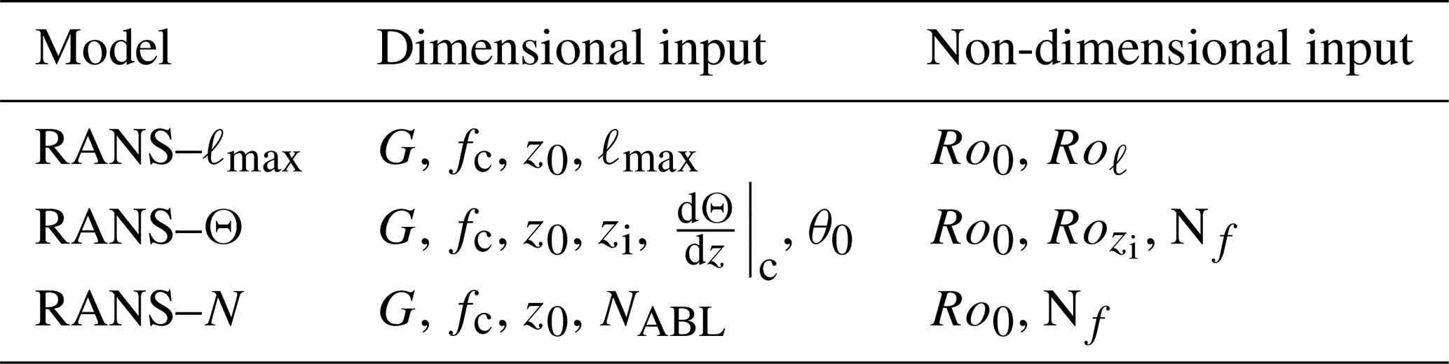
The first dimensionless number is the surface Rossby number, $R{o}_{\mathrm{0}}\equiv G/\left(\right|f_{\mathrm{c}}\left|z_{\mathrm{0}}\right)$, and can be obtained by writing the 1D momentum equations (Eq. 1) in a complex form using $W\equiv (U-U_{\mathrm{G}})+i(V-V_{\mathrm{G}})$, with $i\equiv \sqrt{-\mathrm{1}}$, followed by a substitution of the normalized variables, $z^{\prime }\equiv z/z_{\mathrm{0}}$, $W^{\prime }\equiv W/G$ and ${\mathit{\nu }}_{\mathrm{T}}^{\prime }\equiv {\mathit{\nu }}_{\mathrm{T}}/\left(z_{\mathrm{0}}G\right)$:

$$\begin{array}{}\text{(14)}& R{o}_{\mathrm{0}}{\displaystyle \frac{\mathrm{d}}{\mathrm{d}{z}^{\prime }}}\left({\mathit{\nu }}_{\mathrm{T}}^{\prime }{\displaystyle \frac{\mathrm{d}{W}^{\prime }}{\mathrm{d}{z}^{\prime }}}\right)=i{W}^{\prime }.\end{array}$$

All models that solve the momentum (Eq. 14) follow a Rossby similarity. The other dimensionless numbers are related to the turbulence model (Eq. 2), which can be written in a non-dimensional form using $k^{\prime }=k/G^{\mathrm{2}}$, ${\mathit{\epsilon }}^{\prime }=\mathit{\epsilon }{z}_{\mathrm{0}}/G^{\mathrm{3}}$:

$$\begin{array}{}\text{(15)}& \begin{array}{rl}& {\displaystyle \frac{\mathrm{d}}{\mathrm{d}{z}^{\prime }}}\left({\displaystyle \frac{{\mathit{\nu }}_{\mathrm{T}}^{\prime }}{{\mathit{\sigma }}_k}}{\displaystyle \frac{d{k}^{\prime }}{d{z}^{\prime }}}\right)+{\mathcal{P}}^{\prime }+{\mathcal{B}}^{\prime }-{\mathit{\epsilon }}^{\prime }=\mathrm{0},\\ & {\displaystyle \frac{\mathrm{d}}{\mathrm{d}{z}^{\prime }}}\left({\displaystyle \frac{{\mathit{\nu }}_{\mathrm{T}}^{\prime }}{{\mathit{\sigma }}_{\mathit{\epsilon }}}}{\displaystyle \frac{d{\mathit{\epsilon }}^{\prime }}{d{z}^{\prime }}}\right)+\left(C_{\mathit{\epsilon },\mathrm{1}}^{*}{\mathcal{P}}^{\prime }-C_{\mathit{\epsilon },\mathrm{2}}{\mathit{\epsilon }}^{\prime }+C_{\mathit{\epsilon },\mathrm{3}}{\mathcal{B}}^{\prime }\right){\displaystyle \frac{{\mathit{\epsilon }}^{\prime }}{k^{\prime }}}=\mathrm{0},\end{array}\end{array}$$

with ${\mathcal{P}}^{\prime }\equiv \mathcal{P}{z}_{\mathrm{0}}/G^{\mathrm{3}}$ and ${\mathcal{B}}^{\prime }\equiv \mathcal{B}{z}_{\mathrm{0}}/G^{\mathrm{3}}$. Here, the small ambient source terms are neglected. The additional dimensionless numbers are obtained from non-dimensionalizing either $C_{\mathit{\epsilon },\mathrm{1}}^{*}$ (Eq. 5) or ℬ^′ (via Eqs. 3, 8, 11):

$$\begin{array}{}\text{(16)}& \begin{array}{rl}& \mathrm{RANS}-{\mathrm{\ell }}_{\max }:\\ & {\mathcal{B}}^{\prime }=\mathrm{0},C_{\mathit{\epsilon },\mathrm{1}}^{*}=C_{\mathit{\epsilon },\mathrm{1}}+\left(C_{\mathit{\epsilon },\mathrm{2}}-C_{\mathit{\epsilon },\mathrm{1}}\right)C_{\mathit{\mu }}^{\mathrm{3}/\mathrm{4}}{\displaystyle \frac{{k^{\prime }}^{\mathrm{3}/\mathrm{2}}}{{\mathit{\epsilon }}^{\prime }}}{\displaystyle \frac{R{o}_{\mathrm{\ell }}}{R{o}_{\mathrm{0}}}},\\ & \mathrm{RANS}-\mathrm{\Theta }:\\ & {\mathcal{B}}^{\prime }=-{\displaystyle \frac{{\mathit{\nu }}_{\mathrm{T}}^{\prime }}{{\mathit{\sigma }}_{\mathit{\theta }}}}{\left({\displaystyle \frac{{\mathrm{N}}_f}{R{o}_{\mathrm{0}}}}\right)}^{\mathrm{2}}\left[{\displaystyle \frac{\mathrm{1}}{\mathrm{2}}}+{\displaystyle \frac{\mathrm{1}}{\mathrm{2}}}\tanh \left({\displaystyle \frac{z^{\prime }R{o}_{z_{\mathrm{i}}}/R{o}_{\mathrm{0}}-\mathrm{1}}{z_T/z_{\mathrm{i}}}}\right)\right],\\ & C_{\mathit{\epsilon },\mathrm{1}}^{*}=C_{\mathit{\epsilon },\mathrm{1}},\\ & \mathrm{RANS}-N:\\ & {\mathcal{B}}^{\prime }=-{\displaystyle \frac{{\mathit{\nu }}_{\mathrm{T}}^{\prime }}{{\mathit{\sigma }}_{\mathit{\theta }}}}{\left({\displaystyle \frac{{\mathrm{N}}_f}{R{o}_{\mathrm{0}}}}\right)}^{\mathrm{2}},C_{\mathit{\epsilon },\mathrm{1}}^{*}=C_{\mathit{\epsilon },\mathrm{1}},\end{array}\end{array}$$

where $R{o}_{\mathrm{\ell }}\equiv G/\left(\right|f_{\mathrm{c}}\left|{\mathrm{\ell }}_{\max }\right)$ and $R{o}_{z_{\mathrm{i}}}\equiv G/\left(\right|f_{\mathrm{c}}\left|z_{\mathrm{i}}\right)$ are Rossby numbers based on different ABL length scales, namely, ℓ_max and z_i, respectively. In addition, ${\mathrm{N}}_f\equiv N/\left|f_{\mathrm{c}}\right|$ is the Zilitinkevich number using the Brunt–Väisälä frequency from Eq. (12) using a constant gradient of temperature (representing the inversion or the entire ABL for the RANS–Θ and RANS–N models). Note that one could also replace N_f by a Richardson number, in the form of $({\mathrm{N}}_f/R{o}_{\mathrm{0}}{)}^{\mathrm{2}}$. The similarity of the RANS–ℓ_max and RANS–Θ models has been shown through numerical experiments in previous work (van der Laan et al., 2020, 2023b). The similarity of the ABL models can be employed to create an ABL library numerically for all possible solutions, which can be used to obtain an ABL profile with a desired turbulence intensity and wind speed at a reference height using G and N_ABL (in the case of the RANS–N model) as free parameters, for a given f_c and z₀. The proposed RANS–N model has one fewer dimensional number compared to the RANS–Θ model, which reduces the input parameter space.¹ In addition, all three RANS models can be used to satisfy Reynolds number similarity by keeping their non-dimensional numbers constant. This is an advantage when running wind speed inflow cases consecutively to reduce the total number of required iterations for wind farm AEP simulations (van der Laan et al., 2019, 2022).

3 Numerical methodology

The RANS simulations of the inflow and single-turbine wake are carried out with PyWakeEllipSys (DTU Wind and Energy Systems, 2024), which is Python framework for wind farm CFD simulations. The underlying CFD solver is EllipSys, which is an in-house finite volume code initially developed by Michelsen (1992) and Sørensen (1994). The numerical domain and boundary conditions of the 1D inflow precursor and 3D wind turbine simulations are depicted in Fig. 1 and are further discussed in Sect. 3.1 and 3.2.

3.1 Inflow

The RANS inflow models are solved numerically with EllipSys1D (van der Laan and Sørensen, 2017). A 1D grid with a height of 100 km, a first-cell height of 0.01 m and 768 cells is employed, as shown in Fig. 1a. A relatively tall domain is employed to be able to simulate all possible ABL solutions, as discussed in van der Laan et al. (2020). A rough wall boundary condition from Sørensen et al. (2007) is employed at the ground and depends on the roughness length z₀. At the top, a Neumann condition is applied. Since the 1D RANS equations are stiff, we solve them transiently with a fixed time step of $\mathrm{\Delta }t=\mathrm{1}/f_{\mathrm{c}}$ until a steady-state has been achieved.

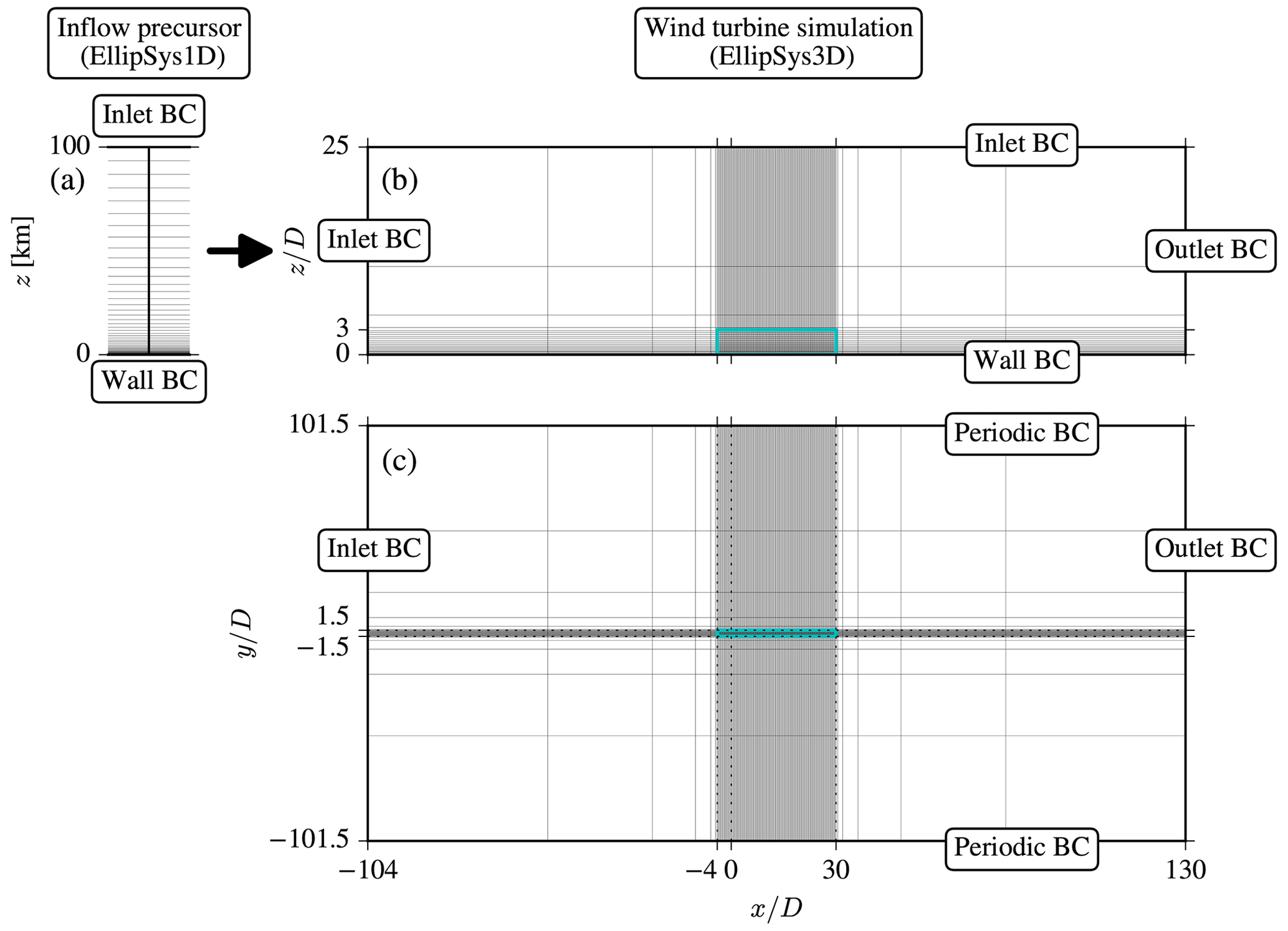
Figure 1 Numerical grid and boundary conditions of the 1D inflow precursor (a) and 3D wind turbine simulations (b–c). The cyan rectangle marks the refined domain around the turbine, and every eighth cell is shown.

3.2 Single wake

The RANS inflow models are applied to RANS single-wake simulations, performed with EllipSys3D. The numerical setup follows a very similar approach to that performed in previous work (van der Laan et al., 2015c) and solves the 3D form of Eqs. (1)–(2). We aim to compare the RANS simulations (both inflow and turbine wakes) with the results of two LES models from Hodgson et al. (2023). These LES models employ an actuator disk (AD) model based on airfoil data to represent the forces of the SWT-2.3-93 turbine (proprietary to Siemens Gamesa Renewable Energy), which has a rated power of 2.3 MW; a rotor diameter, D, of 93 m; and a hub height, z_H, of 68.5 m. Our RANS simulations use the same turbine type, but we employ an AD (Réthoré et al., 2014) including the analytic blade force distribution model of Sørensen et al. (2020), which has shown to compare well with an AD based on airfoil data. In order to perform a fair comparison between the LES and RANS models, we have rerun the LES wake simulations using the same AD model as applied in RANS; see Sect. 3.2.1 for more details. The AD model includes effects of rotor rotation and nonuniform inflow as wind shear and wind veer. In addition, we use a 1D momentum controller (Calaf et al., 2010) similar to one of the LES models from Hodgson et al. (2023) based on the same inputs: a tip speed ratio of 7.75, a thrust coefficient of 0.73, and a power coefficient of 0.45. Note the actual values can differ because a 1D momentum controller typically overestimates the freestream wind speed and thrust force, as shown in previous work (van der Laan et al., 2015b). The effective values of the power and thrust coefficients based on the disk-averaged streamwise velocity are set as 1.026 and 1.264, respectively.

A Cartesian domain is employed with dimensions $\mathrm{234}D\times \mathrm{203}D\times \mathrm{30}D$ for the streamwise (x), lateral (y), and vertical (z) directions, respectively, as depicted in Fig. 1a–b. The large domain extent is used to minimize the effect of numerical blockage. An inner domain around the turbine, located at $(x,y,z)=(\mathrm{0},\mathrm{0},z_{\mathrm{H}})$, is used to resolve the wind turbine wake with a fine uniform spacing of $D/\mathrm{32}$ (cyan rectangle in Fig. 1a–b). The inner domain has the following horizontal dimensions: $-\mathrm{4}D<x<\mathrm{30}D$ and $-\mathrm{1.5}D<y<\mathrm{1.5}D$. Vertically, the cell sizes are growing with z using a first-cell height of $D/\mathrm{200}$, a maximum cell size of $D/\mathrm{32}$ at z=3D, and a maximum expansion ratio of 1.2. Above z=3D, the cells continue to grow with a similar expansion ratio. The total number of cells is 43.6 million. The effect of coarser grid spacing is shown in Appendix B. An inlet boundary condition is at the inflow boundary ($x=-\mathrm{104}D$) and at the top of domain (z=25D). The bottom boundary is a rough wall boundary condition (Sørensen et al., 2007). The lateral boundaries ($y=\pm \mathrm{101.5}D$) are periodic because of the presence of wind veer. A Neumann condition is set at the outflow boundary (x=130D). More details of the numerical setup are discussed in van der Laan et al. (2015c) with the exception of the lateral boundaries, which are set to periodic boundary conditions because of the presence of wind veer.

3.2.1 LES

The LES results of Hodgson et al. (2023) are used to compare to our RANS models results for both the inflow and single-wake cases. Hodgson et al. (2023) employed two different LES models: WiRE (Albertson and Parlange, 1999; Porté-Agel et al., 2000; Wu and Porté-Agel, 2011) and EllipSys3D (the same solver used for the RANS simulations), here labeled as LES–EPFL and LES–DTU, respectively. In order to provide a fair comparison with the RANS models, we have rerun the LES–DTU single-wake cases following the same methodology as Hodgson et al. (2023) but using a finer grid spacing of $D/\mathrm{32}$ around the AD instead of $D/\mathrm{16}$. In addition, we have extended the refined domain around the AD in the streamwise direction to 30D for the SBL inflow case, such that we can compare LES–DTU results of the far wake with RANS. Furthermore, we have extended the precursor simulation by an additional 2 h such that the LES–DTU stable boundary layer (SBL) single-wake simulation can be averaged over 3 h in order to obtain converged statistics in the far wake. Finally, we employ the same AD model as used in the RANS simulations including a 1D momentum controller for both inflow cases.

3.3 Wind turbine row with SBL inflow

The SBL inflow case is also applied to a small wind farm consisting of a row of five SWT-2.3-93 turbines (the same turbine used for the single-wake cases) with 5D spacing. The RANS wind farm domain is similar to the domain used for the single-wake cases (as depicted in Fig. 1). However, a larger inner domain is used with the following horizontal dimensions: $-\mathrm{4}D<x<\mathrm{40}D$ and $-\mathrm{3.5}D<y<\mathrm{3.5}D$, leading to a total number of 94.4 million cells. The wind turbine row subjected to the SBL inflow case is also simulated with the LES–DTU model using the same extended domain as used for the SBL single-wake case, as discussed in Sect. 3.2.1.

4 Results and discussion: a comparison with LES

4.1 Inflow

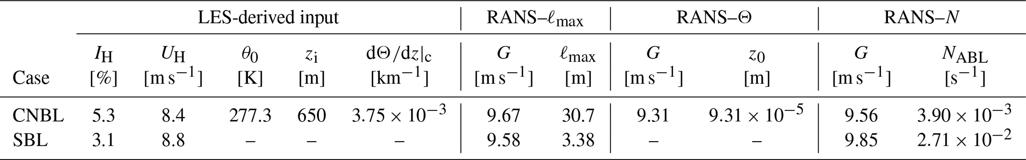
The two existing and proposed RANS inflow models from Sect. 2 are applied to two ABL cases based on LES results from Hodgson et al. (2023), who used two different LES models. The ABL cases represent a CNBL and a stable ABL (SBL) inspired by the LES intercomparison study from Beare et al. (2006). The LES models from Hodgson et al. (2023) are employed with $f_{\mathrm{c}}=\mathrm{1.185}\times {\mathrm{10}}^{-\mathrm{4}}$ s⁻¹ and z₀=0.001 m. The values of the Coriolis parameter correspond to a latitude of 54.3°, and it is based on the location of the Danish offshore wind farm, Rødsand II. While we adopt the value of f_c from Hodgson et al. (2023), a lower roughness length is used in the RANS models. This is because the RANS models use C_μ=0.03, while the LES models imply a higher effective C_μ based on the turbulent kinetic energy and friction velocity near the wall, as shown in Baungaard et al. (2024). This is compensated for using a lower roughness length of z₀=0.0002 m in the RANS–ℓ_max and RANS–N models. Note that if a higher C_μ were set in the RANS models, then the other turbulence model constants would need to be adjusted and calibrated, which is not within the scope of the present article. The RANS inflow models use G and an additional parameter to obtain the turbulence intensity based on k; I_H; and wind speed, U_H, at the reference height of 68.5 m – namely, ℓ_max, z₀, and N_ABL for RANS–ℓ_max, RANS–Θ, and RANS–N, respectively. The LES-derived input parameters and fitted RANS inflow model parameters are listed in Table 2. The RANS–ℓ_max and RANS–N models use pre-calculated libraries of all possible ABL solutions that depend on two non-dimensional numbers (as discussed in Sect. 2.4) to look up the values for G and an ABL scale (ℓ_max or N_ABL) for a given set of I_H and U_H. The RANS–Θ model uses an optimizer to find the values of G and z₀ for the CNBL case. LES-diagnosed values of θ₀, z_i, and $\mathrm{d}\mathrm{\Theta }/\mathrm{d}z{|}_{\mathrm{c}}$ are not necessary for the SBL case because we do not employ the RANS–Θ model for this case.

Table 2 LES-derived input from ABL cases and fitted parameters of RANS inflow models.

The RANS inflow model results are compared with the two LES models from Hodgson et al. (2023) for the CNBL and SBL cases in Fig. 2. The results of the LES models compare well with the results of the RANS–ℓ_max and RANS–N models in terms of wind speed and turbulence intensity based on k ($I_k=\sqrt{\mathrm{2}/\mathrm{3}k}/\sqrt{U^{\mathrm{2}}+V^{\mathrm{2}}}$) for both ABL cases (Fig. 2a, c, g and i). The good fit around the hub height is expected since the RANS models are tuned for the LES-predicted values of I_H and U_H. The RANS-predicted wind veer as shown by the relative wind directions in Fig. 2b and h also compares well with both LES models for the CNBL case. However, the RANS–ℓ_max and RANS–N models predict stronger wind veer over the rotor area (11.1 and 12.7°, respectively) compared to the LES models (8.8 and 9.9° for DTU and EPFL, respectively) for the SBL case. The main differences between the RANS models are the profiles of turbulence length scale (Fig. 2d, j) and eddy viscosity (Fig. 2e and k), where the RANS–ℓ_max model predicts taller ABLs compared to the RANS–N model; the veer difference is due in part to different effective ABL heights (Kelly and van der Laan, 2023).

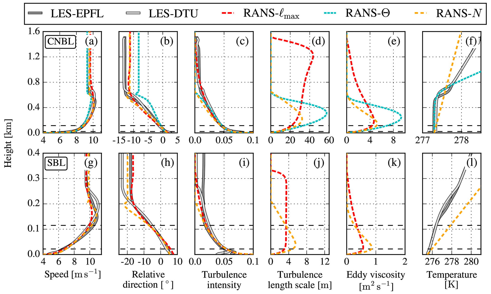
Figure 2 RANS-simulated ABL inflow compared to LES model results from Hodgson et al. (2023) for CNBL (a–f) and SBL inflow cases (g–l). Horizontal dashed lines represent the rotor-swept area of the SWT-2.3-93 wind turbine.

Note that it is not trivial to postprocess an eddy viscosity or turbulence length scale from the LES data that can be directly compared to the RANS models. This is because one would need additional modeling to obtain an eddy viscosity implied by the LES data. Furthermore, the RANS turbulence length scale is a model definition, while an LES-derived turbulence length scale can be ambiguous and is only qualitatively comparable (van der Laan and Andersen, 2018) unless non-Boussinesq contributions are accounted for (e.g., Large et al., 2019). For the SBL case, it is clear that the turbulence length scale in the RANS–ℓ_max model is limited to a maximum value of 3.4 m, while the turbulence length scale of the RANS–N model results in a smoother profile that has a higher value in the surface layer but a lower value around the ABL height. As a result, the profiles of wind speed and direction around the ABL height are more diffused in the RANS–ℓ_max model compared to the RANS–N model, which is most visible for the SBL case (Fig. 2g and h) around z=0.2 km. In other words, RANS–N has a more pronounced Ekman layer. The RANS–N model predicts a lower ABL height compared to the LES models for both ABL cases, but this could be improved by lowering the applied roughness length. The latter is not performed in order to provide a fairer comparison between the RANS–N and RANS–ℓ_max models using the same roughness length. The RANS–Θ model compares well with the LES models for the CNBL case but shows a larger turbulence length scale and eddy viscosity compared to the RANS–N model due to zero turbulent buoyancy in the surface layer (Fig. 2d and e). The RANS–Θ model is not applied to the SBL case because the RANS–Θ model cannot represent an SBL or a shallow CNBL, as discussed in Appendix A. Results of the implied temperature profile of the RANS–N model, $\mathrm{\Theta }\left(z\right)/{\mathit{\theta }}_{\mathrm{0}}=\mathrm{1}+z{N}_{\mathrm{ABL}}^{\mathrm{2}}/g$, are shown in Fig. 2f and l. It is clear that the temperature gradient employed is larger in the RANS–N with respect to the LES models, although a direct comparison with LES in terms of a temperature profile may not be fair due to the simplicity of the RANS–N model. In addition, the choice of the turbulent Prandtl number in Eq. (11), here σ_θ=1, will also determine the implied temperature gradient of the RANS–N model because it influences the obtained value of N_ABL. One could match a constant temperature gradient to the LES results, however, it is not guaranteed that the RANS–N model will compare well with the LES results in terms of wind speed, direction, and turbulent intensity profiles.

4.2 Single wake

The RANS inflow models are applied to single-turbine wake simulations, and the results of velocity deficit magnitude and wake-added turbulence intensity are compared with results from the two LES models of Hodgson et al. (2023) in Fig. 3. The wake results are normalized by the simulation results without a turbine. The RANS–Θ model is only applied to the CNBL case and not to the SBL case because the model cannot represent a shallow ABL, as discussed in Appendix A. The CNBL case shows that all three RANS inflow models predict similar velocity deficits that follow the trends of the LES models (Fig. 3b–d). The differences between the RANS and LES models in the near wake at x=1D (Fig. 3a) are expected, following a previous study (van der Laan et al., 2015c). The difference in velocity deficit between the RANS and LES models for the SBL case is larger than that for the CNBL case. The largest difference between the RANS–ℓ_max and RANS–N models is observed at the far wake at x=25D for the SBL case, which is depicted in Fig. 4. Figure 4a shows that the RANS–ℓ_max model does not allow the turbine wake to recover vertically with respect to the RANS–N model due to the global length-scale limiter. The LES results at x=25D suggest that the RANS–N model predicts the vertical wake recovery better, although the magnitude of the velocity deficit is captured slightly better by RANS–ℓ_max. A future study is needed to further validate the results of the RANS–N model for additional LES cases that differ in atmospheric conditions.

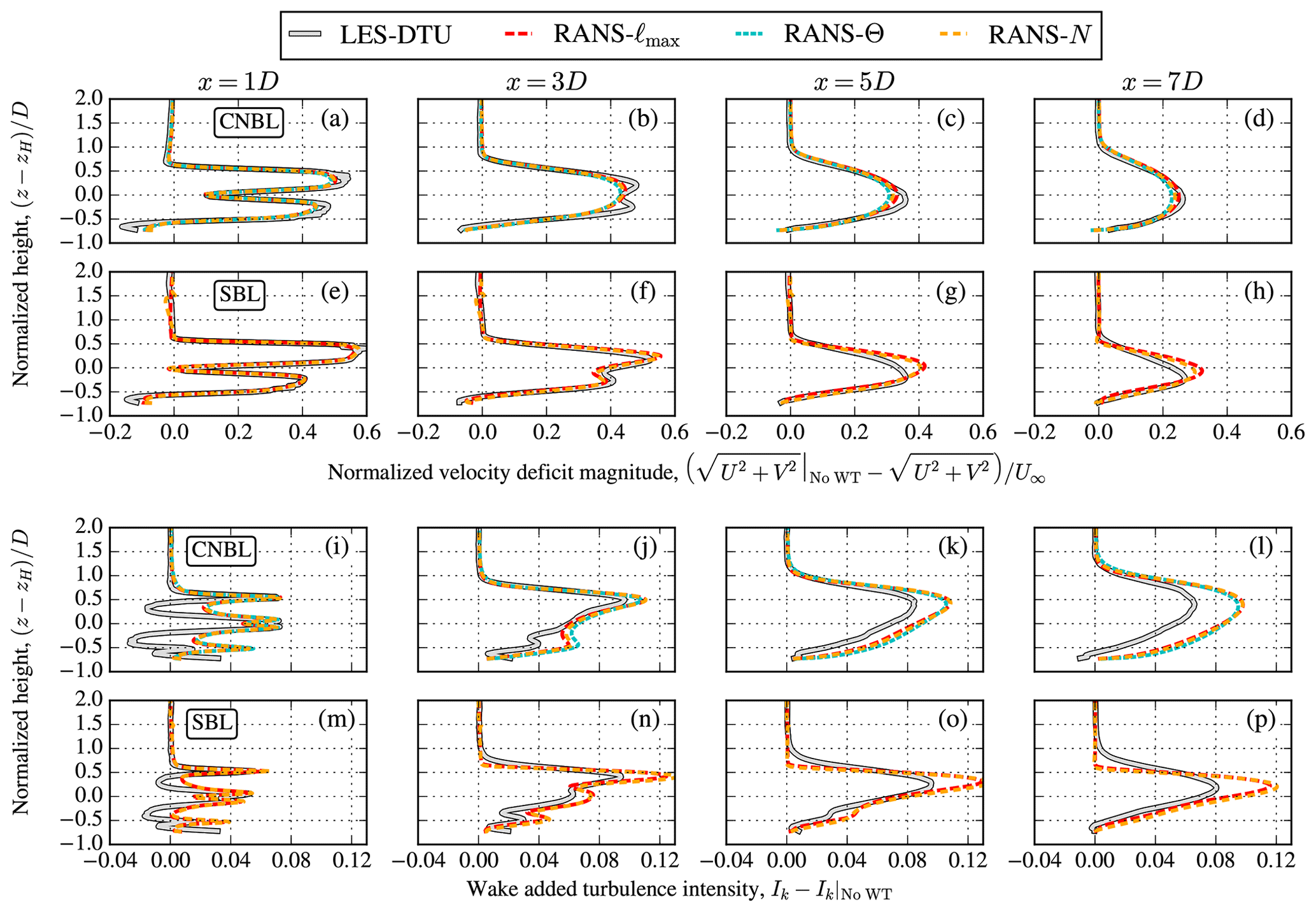
Figure 3 RANS-simulated wake velocity deficit (a–h) and wake-added turbulence intensity (i–p) compared to LES model results, for the CNBL (a–d, i–l) and SBL inflow cases (e–h, m–p). LES wake-added turbulence intensity includes resolved and sub-grid model results.

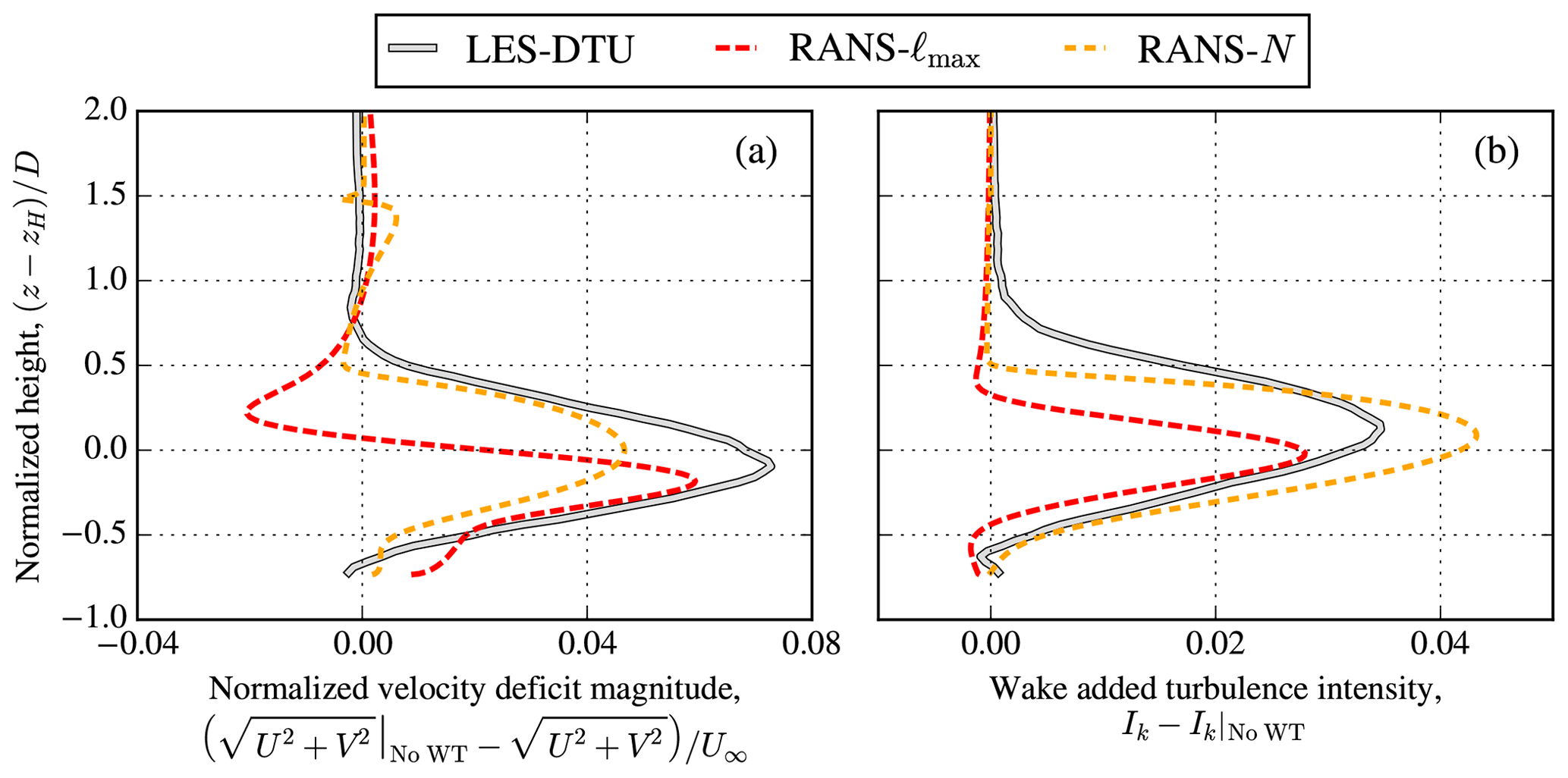
Figure 4 RANS-simulated wake velocity deficit (a) and wake-added turbulence intensity (b) compared to LES–DTU model results for the far wake at x=25D of the SBL inflow case. LES wake-added turbulence intensity includes resolved and sub-grid model results.

The RANS–N model results of the SBL single-wake case shows a small speedup around the ABL height $(z-z_{\mathrm{H}})/D\approx \mathrm{1.4}$ at x=1D (Fig. 3e), which grows further downstream (Figs. 3f–h and 4a). This is a numerical issue associated with the low eddy viscosity at the ABL height that can also occur with the other RANS inflow models, especially when they are applied to a large wind farm (van der Laan et al., 2023b). A possible solution is an additional damping method in the momentum equation. Since the proposed RANS–N model does not limit the turbulence length scale globally, one could add a high-eddy-viscosity damping layer above the ABL through additional sources of k and ε in the transport equations. Such a damping layer can presumably be made to not influence the inflow profiles, while still damping the numerical “wiggles” in the wind turbine simulation. The required amount of damping is case-dependent and needs further study, which is part of ongoing work.

None of the RANS models are able to predict the wake-added turbulence intensity compared to LES (Fig. 3i–p) because of the applied isotropic Boussinesq hypothesis. However, the RANS models do not need a good prediction of wake-added turbulence intensity in order to predict a realistic velocity deficit because the wake recovery is dictated by the divergence of the shear stresses (van der Laan et al., 2023a); the latter can be modeled well by the isotropic Boussinesq hypothesis and a variable C_μ (for example through f_P).

Contours of the streamwise velocity and eddy viscosity at hub height of the SBL single-wake case are shown in Fig. 5 for the RANS–N and RANS–ℓ_max models. Two results of the RANS–ℓ_max model are shown, one with and one without the blending function of Eq. (6) that is used to switch off the global turbulence length-scale limiter in the wake region (identified by the f_P function). Without Eq. (6), the eddy viscosity does not increase significantly because of the global turbulence length-scale limiter (Fig. 5e), which delays the recovery of the streamwise velocity deficit and shows a speedup region in the far wake (Fig. 5a). When Eq. (6) is included, the eddy viscosity can increase downstream, but it quickly returns to the ambient eddy viscosity in the region where f_P is close to 1 (Fig. 5f). The RANS–N model does not limit the turbulence length scale as the RANS–ℓ_max model, which results in a smoothly increasing (up to x=10D) and decreasing eddy viscosity (Fig. 5g). As a result, a smoother far-wake velocity deficit is obtained by the RANS–N model (Fig. 5c), which explains the difference between the RANS–ℓ_max and RANS–N models at x=25D shown in Fig. 3j. In addition, the streamwise velocity of the LES–DTU model (Fig. 5d) compares better with the results of RANS–N than RANS–ℓ_max up to a distance of about 20D downstream. Further downstream, RANS–N predicts less velocity deficit at hub height compared to LES, as shown previously in Fig. 4a.

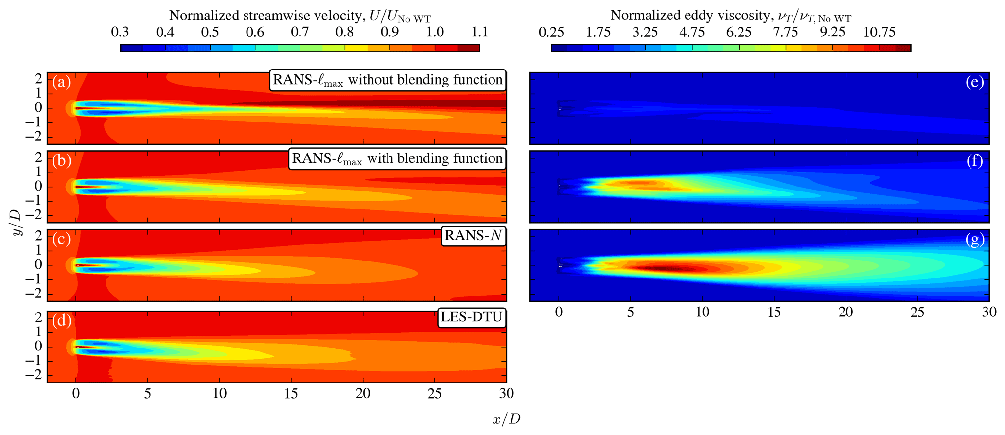
Figure 5 Hub height contours of normalized streamwise velocity (a–d) and wake eddy viscosity normalized by inflow eddy viscosity (e–f) for the SBL case. RANS–ℓ_max model without the blending function of Eq. (6) (a, e), RANS–ℓ_max model with the blending function of Eq. (6) (b, f), RANS–N model (c, g), and the LES–DTU model (d).

4.3 Wind turbine row with SBL inflow

Simulation results of a wind turbine row consisting of five turbines with 5D spacing in the streamwise direction, subjected to the SBL inflow, are depicted in Figs. 6–8. Contours of normalized streamwise velocity are shown in Figs. 6a–d and 7 at hub height and at five cross-planes, respectively, for the RANS and LES–DTU models. Two results of the RANS–ℓ_max are shown, similar to the single-wake results in Fig. 5. Without the blending function, the wake recovery inside the wind turbine row is slow (Fig. 6a) because the eddy viscosity is not growing downstream due to the global length-scale limiter (Fig. 6e). In addition, the global length-scale limiter also affects the vertical-wake recovery, leading to wake shapes (Fig. 7b–e) that do not resemble the LES results at all (Fig. 7q–t). When the blending function is used (Fig. 6b), the wakes of the first turbines are more comparable with the LES results (Fig. 6d); however, further downstream the wake recovery is again too slow because the blending function is less active at this distance, resulting in low eddy viscosity (Fig. 6f) and artificial wake shapes (Fig. 7h–j). The RANS–N model predicts an eddy viscosity that is smooth and grows with downstream distance (Fig. 6g). As a result, the wake recovery of the RANS–N model (Fig. 6c) is faster than RANS–ℓ_max (Fig. 6b), and the wake shapes of the RANS–N model (Fig. 7l–o) more closely resemble the LES results (Fig. 7q–t). However, the magnitude of the streamwise velocity deficit predicted by the RANS–N model (Fig. 6c) is underpredicted compared to the results of the LES–DTU model (Fig. 6d). In addition, the wakes of the LES–DTU simulations are more deflected compared to the wakes of the RANS–N model.

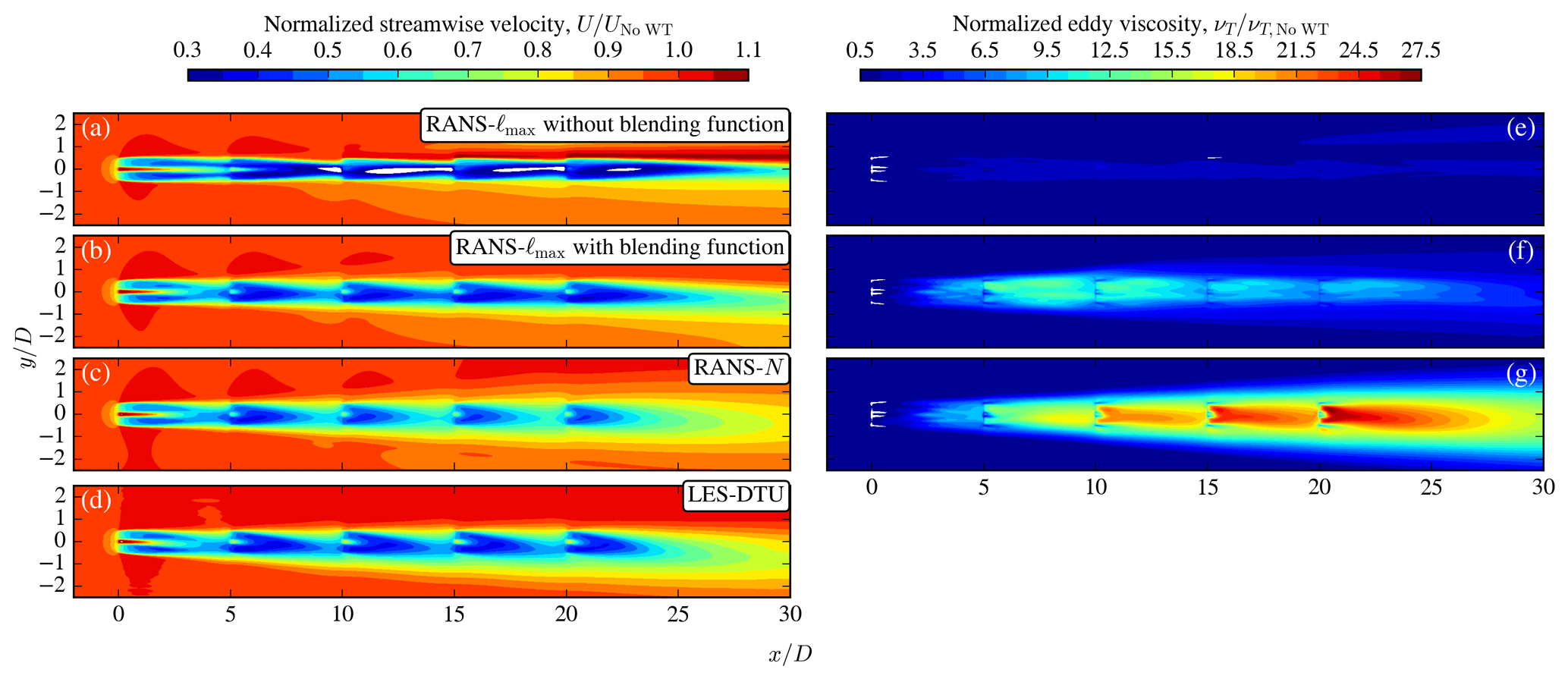
Figure 6 Hub height contours of normalized streamwise velocity (a–d) and wake eddy viscosity normalized by inflow eddy viscosity (e–f) for the SBL case applied to a wind turbine row. RANS–ℓ_max model without the blending function of Eq. (6) (a, e), RANS–ℓ_max model with the blending function of Eq. (6) (b, f), RANS–N model (c, g), and the LES–DTU model (d).

Figure 7 Cross-plane contours of normalized streamwise velocity for the SBL case applied to a wind turbine row. RANS–ℓ_max model without the blending function of Eq. (6) (a–e), RANS–ℓ_max model with the blending function of Eq. (6) (f–j), RANS–N model (k–o), and the LES–DTU model (p–t).

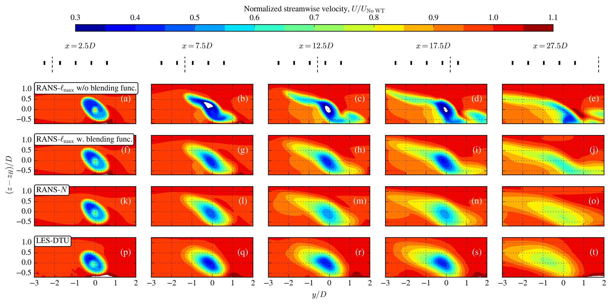
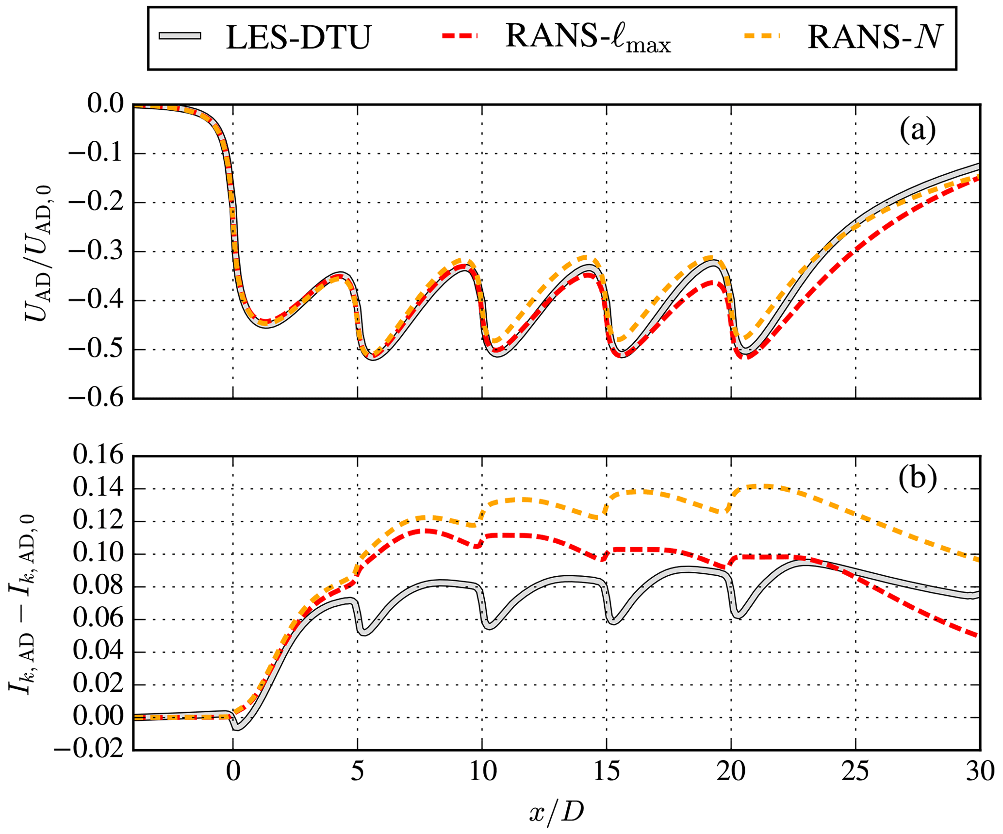
Figure 8 Rotor-averaged streamwise velocity deficit (a) and wake-added turbulence intensity (b) normalized by their respective values at $x=-\mathrm{4}D$, for the SBL case, applied to a wind turbine row simulated by the RANS and LES–DTU models. LES wake-added turbulence intensity includes resolved and sub-grid model results.

Figure 8 depicts results of the streamwise velocity deficit and wake-added turbulence intensity as rotor-averaged values along the turbine row. The RANS–ℓ_max model performs best inside the wind turbine row, while the RANS–N model performs better behind the last turbine, in terms of matching the velocity deficit from the LES–DTU; this is shown in Fig. 8a. It should be noted that the LES–DTU model predicts a stronger wake deflection compared to the RANS models (as discussed previously with Fig. 6), which can affect the comparison in terms of rotor-averaged results. In terms of wake-added turbulence intensity (Fig. 8b), neither RANS model can predict the LES results. It is also clear that the DTU–LES model predicts a loss in wake-added turbulence intensity at the actuator disk locations. Such behavior has also been observed in other LES–AD simulation results (Abkar and Porté-Agel, 2015; García-Santiago et al., 2024). Zehtabiyan-Rezaie and Abkar (2024) proposed an additional sink of k in a RANS–AD model in order to mimic the LES–AD results (without the use of an f_P function). The proposed RANS–N model could potentially be extended with a similar additional sink of k, although it is unclear if a reduction in turbulent kinetic energy at the rotor is a real phenomenon or a model artifact (e.g., related to representing a rotor as an AD where blade-resolved turbulence is absent). Alternatively, the f_P function (Eq. 2) could be recalibrated for stable conditions such that the diffusivity of the RANS–N model is reduced. A similar exercise was performed in a previous work to model a wind turbine wake under unstable surface-layer conditions (Baungaard et al., 2022a). A further development of the RANS–N model requires a range of inflow cases applied to wind farms using LES. In addition, the RANS–N model needs to be validated with field measurements.

5 Conclusions

A new RANS inflow model of the neutral and stable ABL is proposed and compared with two existing RANS inflow models for CNBL and SBL cases based on LES model results. The proposed inflow (RANS–N) model does not require a global length-scale limiter or prior knowledge of a temperature profile by the use of simple turbulent buoyancy expression based on a constant Brunt–Väisälä frequency. The RANS–N model compares well with LES-predicted profiles of wind speed, wind direction, and turbulence intensity. The simplicity of the RANS–N model results in a reduced parameter space consisting of only two non-dimensional numbers: the surface Rossby number and the Zilitinkevich number. The three RANS inflow models are applied to single wind turbine wakes for the same ABL cases, and their simulated velocity deficit compares well with results from LES for the CNBL case. In addition, the SBL inflow case is applied to an along-wind turbine row. The present study has shown that the proposed RANS–N model is better-suited to simulate the effect of a shallow SBL on a single wind turbine wake and a wind turbine row than the existing state-of-the-art RANS–ℓ_max (Apsley and Castro, 1997) and RANS–Θ (van der Laan et al., 2023b) models in terms of the velocity deficit shape. However, the RANS–N model underpredicts the magnitude of the velocity deficit of the wind turbine row with respect to LES, and further model investigation is required. In addition, the interaction of a shallow ABL and a turbine wake in RANS can lead to small numerical wiggles, which grow with downstream distance and need further investigation for the application of large wind farm simulations.

Appendix A: Caveat regarding use of RANS–Θ inflow model with k−ϵ closure

The RANS–Θ model can predict a double ABL height if a strange combination of input parameters is chosen; this happens if the k–ϵ model implies a value of z_i significantly different from that chosen in the temperature profile Θ(z). For example, for a shallow ABL one could set a low z_i, but if the chosen inversion strength is not strong enough then the effective ABL height can occur above the inversion height, z>z_i. An example of this issue is shown in Fig. A1, where the RANS–Θ model is employed for $\left\{G,f_{\mathrm{c}},z_{\mathrm{0}},z_{\mathrm{i}},\mathrm{d}\mathrm{\Theta }/\mathrm{d}z{|}_{\mathrm{c}}\right\}=\left\{\mathrm{10}\mathrm{m},{\mathrm{10}}^{-\mathrm{4}}{\mathrm{s}}^{-\mathrm{1}},{\mathrm{10}}^{-\mathrm{4}}\mathrm{m},\mathrm{100}\mathrm{m},\mathrm{0.1}{\mathrm{Km}}^{-\mathrm{1}}\right\}$ and three different combinations of $z_T/z_{\mathrm{i}}$. The earlier prescribed value ($z_T/z_{\mathrm{i}}=\mathrm{0.2}$) can result in the double-height problem, which creates an inflection point in the wind speed profile (Fig. A1a) at z≈80 m. When the smoothing is increased by setting larger values of $z_T/z_{\mathrm{i}}$, then the double ABL height is less visible, and the model behaves more like the RANS–N model since the temperature gradient approaches a constant value.

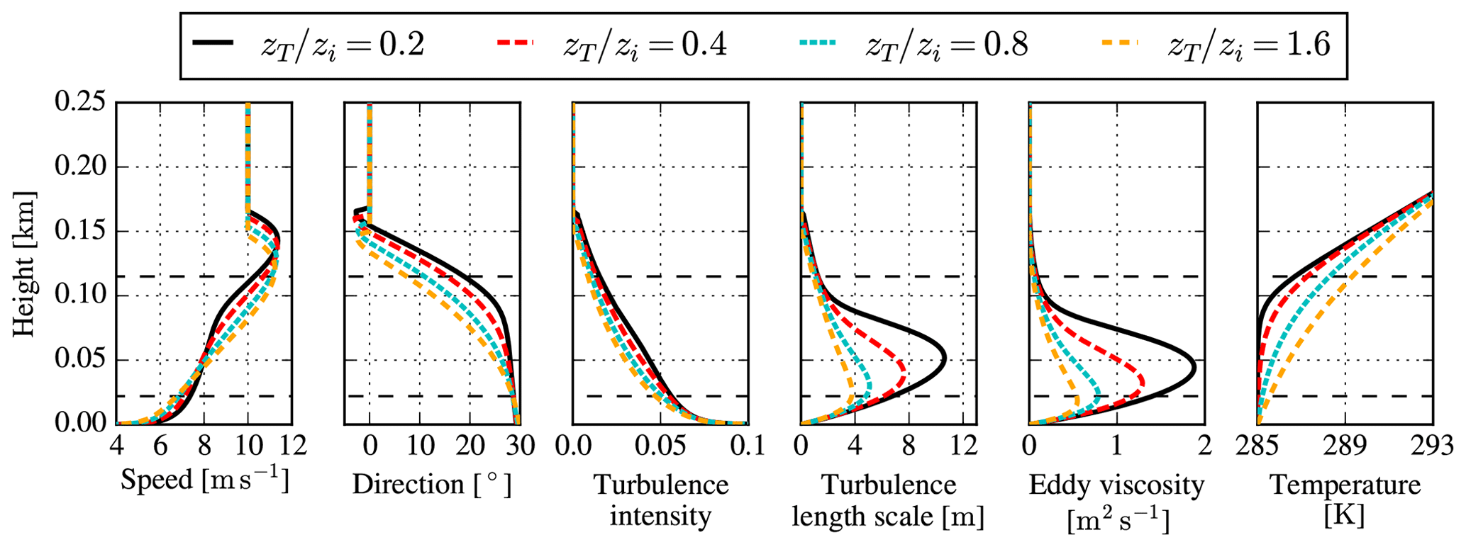
Figure A1 ABL inflow simulated with the RANS–Θ model for different values of $z_T/z_{\mathrm{i}}$. Horizontal dashed lines represent the rotor-swept area of the SWT-2.3-93 wind turbine.

One could extend the RANS–Θ model by adding a surface-layer temperature gradient, $\mathrm{d}\mathrm{\Theta }/\mathrm{d}z{|}_{\mathrm{s}}$:

$$\begin{array}{}\text{(A1)}& \begin{array}{rl}& {\displaystyle \frac{\mathrm{d}\mathrm{\Theta }}{\mathrm{d}z}}={\displaystyle \frac{\mathrm{1}}{\mathrm{2}}}\left[\mathrm{1}+\tanh \left({\displaystyle \frac{\mathrm{1}-z/z_{\mathrm{i}}}{z_T/z_{\mathrm{i}}}}\right)\right]{\left.{\displaystyle \frac{\mathrm{d}\mathrm{\Theta }}{\mathrm{d}z}}\right|}_{\mathrm{s}}\\ & +{\displaystyle \frac{\mathrm{1}}{\mathrm{2}}}\left[\mathrm{1}+\tanh \left({\displaystyle \frac{z/z_{\mathrm{i}}-\mathrm{1}}{z_T/z_{\mathrm{i}}}}\right)\right]{\left.{\displaystyle \frac{\mathrm{d}\mathrm{\Theta }}{\mathrm{d}z}}\right|}_{\mathrm{c}},\end{array}\end{array}$$

which can reduce the problem with double ABL heights for a shallow and stable ABL using a positive surface layer gradient. However, the user can still obtain a double ABL height if $\mathrm{d}\mathrm{\Theta }/\mathrm{d}z{|}_{\mathrm{s}}$ is not strong enough, and for a too-strong $\mathrm{d}\mathrm{\Theta }/\mathrm{d}z{|}_{\mathrm{s}}$, the model can produce a lower ABL height than intended. One could also employ a prescribed temperature gradient profile from a higher-fidelity model as LES; however, a smooth wind speed profile is not guaranteed – research is ongoing on how to ensure such a profile. In the present work, we do not use Eq. (A1) but rather adapt the original formulation (van der Laan et al., 2023b).

Appendix B: Grid refinement study of the RANS–N inflow model applied to the SBL single-wake case

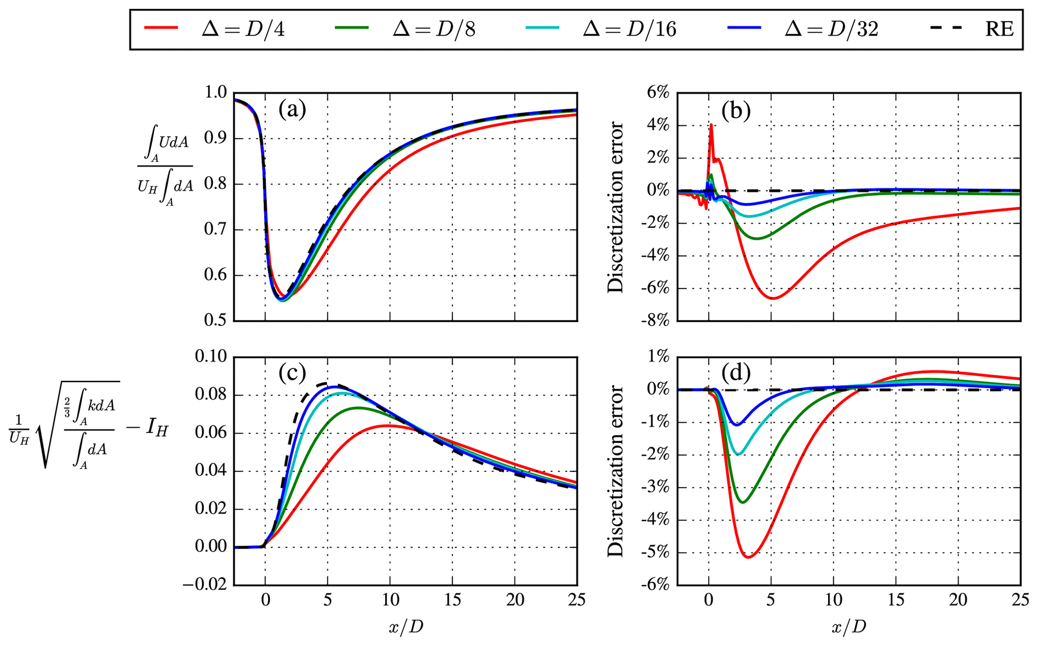
Figure B1 RANS wake streamwise velocity (a) and wake-added turbulence intensity (c), integrated over a fictitious rotor area and corresponding discretization error (b, d) simulated by the RANS–N model for different grid resolutions for the SBL inflow case.

The grid sensitivity of the proposed RANS–N inflow model applied to the single-wake SBL case is depicted in Fig. B1. Three coarser grids are employed compared to the results presented in the main body of the article, which leads to four different grid sizes in the domain around the turbine, Δ: $D/\mathrm{4}$, $D/\mathrm{8}$, $D/\mathrm{16}$, and $D/\mathrm{32}$, which correspond to total cell counts of 0.786, 3.24, 9.96, and 43.6 million, respectively. Figure B1a shows the rotor-integrated streamwise velocity normalized by the freestream and also includes a Richardson extrapolated (RE) value following the mixed-order grid convergence analysis from Roy (2003). The corresponding discretization error (normalized by the freestream velocity) is plotted in Fig. B1b and indicates that a grid spacing of $D/\mathrm{8}$ results in an error of less than 1 % at a downstream distance of 8.5D and beyond. Such an error is acceptable for the application of RANS wind farm simulations of modern offshore wind farms, where the typical turbine interspacing is around 7–10D. The rotor-integrated wake-added turbulence intensity and corresponding discretization error are plotted in Fig. B1c and d, respectively. The errors in wake-added turbulence intensity are of a similar magnitude to the error in the velocity deficit. A grid spacing of $D/\mathrm{8}$ results in an error of about 0.5 % at a downstream distance of 7.5D.