the Creative Commons Attribution 4.0 License.
the Creative Commons Attribution 4.0 License.
 | 16 Feb 2024
Development and application of a mesh generator intended for unsteady vortex-lattice method simulations of wind turbines and wind farms
Luis R. Ceballos
Marcos L. Verstraete
Cristian G. Gebhardt
In the last decades, the unsteady vortex-lattice method (UVLM) has gained a lot of acceptance to study large onshore–offshore wind turbines (WTs). Furthermore, and due to the development of more powerful computers, parallelization strategies, and algorithms like the fast multipole method, it is possible to use vortex-based methods to analyze and simulate wind farms (WFs). However, UVLM-based solvers require structured meshes, which are generally very tedious to build using classical mesh generators, such as those utilized in the context of finite element methods (FEMs). Wind farm meshing is further complicated by the large number of design parameters associated with the wind turbine (coning angle, tilt angle, blade shape, etc.), farm layout, modeling of the terrain topography (for onshore WFs), and modeling of the sea level surface (for offshore WFs), which makes the use of FEM-oriented meshing tools almost inapplicable.
In the literature there is a total absence of meshing tools when it comes to building aerodynamic grids of WTs and WFs to be used along with UVLM-based solvers. Therefore, in this work, we present a detailed description of the geometric modeling and computational implementation of an interactive UVLM-oriented mesh generator, named UVLMeshGen, developed entirely in MATLAB® and easily adaptable to GNU OCTAVE, for wind turbines and onshore–offshore wind farms. The meshing tool developed here consists of (i) a geometric processor in charge of designing and discretizing an entire wind farm and (ii) an independent module in charge of computing the kinematics for the entire WF. The output data provided by the UVLMeshGen consist of nodal coordinates and connectivity arrays, making it especially attractive and useful to be used by other flow potential solvers using vortices, sources and sinks, or dipoles/doublets, among others. The work is completed by providing a series of aerodynamic results related to WTs and WFs to show the capabilities of the mesh generator, without going into detailed discussions of wind turbine aerodynamics, which are not the focus of this paper. The meshing tool developed here is freely available under a Creative Commons Attribution 4.0 International License (Roccia, 2023).
- Article
(28694 KB) - Full-text XML
- BibTeX
- EndNote


For some years now, wind energy has become one of the fundamental pillars on the world stage of renewable energy. This fact has been materialized by an increasing number of different wind turbine (WT) designs: going from small wind turbines like the Vestas V27 of 200 KW (Torabi, 2022) and moderately sized designs for onshore applications to the current large offshore WTs such as the Vestas V236-15.0MW prototype (Vestas, 2022) or the CSSC Haizhuang H260-18MW concept design with a rotor diameter of 260 m (CSSC Haizhuang, 2023).
One of the most important challenges of wind turbine technology is the accurate characterization of the WT loads under inflow conditions that trigger complex aerodynamic effects. Although the description of the flow surrounding a wind turbine has been a subject of interest for many years, the study of three-dimensional and expensive-to-model unsteady aerodynamics of WTs and wind farms is still an active field of research (Muñoz-Simón et al., 2022). Throughout the years, a wide variety of aerodynamic models for wind turbines have been proposed, implemented, verified, validated, and successfully applied. They range from basic approaches such as those based on blade element momentum (BEM) theory, widely spread through the industry for the initial design loops, to advanced high-fidelity models using computational fluid dynamics (CFD) techniques.
While classical and enhanced versions of BEM-based solvers have been found to provide good agreement with measurements and CFD simulations, they require a series of engineering corrections to model challenging unsteady aerodynamic phenomena of increasingly large WTs (Perez-Becker et al., 2020). The inaccuracies observed in BEM simulations, when compared to more sophisticated approaches, are a natural consequence of the underling theory behind the method (Hansen, 2015). Instead, high-fidelity CFD computations can capture more flow physics, thus providing a better prediction accuracy than BEM codes (Nigam et al., 2017; Liu et al., 2017). However, solving the full Navier–Stokes equations for three-dimensional unsteady flows with boundaries undergoing large and complex motion is by far a challenging and time-consuming task requiring typically 2–5 weeks on average (Terry, 2018).
As an intermediate option between the BEM and CFD approaches, we introduce the potential flow solvers, among which the so-called vortex-lattice methods (VLMs) represent a good alternative to assess the aerodynamic performance of different aeronautical–mechanical engineering applications. Its extension to the study of transient aerodynamic loads for slender lifting surfaces undergoing complex motions, the well-known nonlinear unsteady vortex-lattice method (UVLM), has proven to be a more than viable option, presenting an excellent trade-off between precision and computational cost (Verstraete et al., 2023). Furthermore, UVLM-based solvers have been continuously gaining ground in the context of those problems, in which free-wake methods become a necessity due to the geometric complexity and the presence of large displacement–rotations, such as morphing wings (Verstraete et al., 2015, 2019), flapping wings (Stanford and Beran, 2010; Roccia et al., 2013; Nguyen et al., 2016), rotorcraft (Wie et al., 2009; Colmenares et al., 2015; Lee et al., 2022), wind turbines (van Garrel, 2003; Gebhardt et al., 2010; Gebhardt and Roccia, 2014), and non-conventional wind energy devices (Abdelkefi et al., 2014; Beltramo et al., 2020; Roccia et al., 2020), among others.
Among the most promising UVLM-based solvers capable of performing aerodynamic analysis of wind turbines, we can mention OpenVOGEL (Hazebrouck, 2023), WinDS (WinDS, 2023), GSF-Aero (Verstraete et al., 2023), the general-purpose framework developed by Pérez Segura et al. (2020), and VLMSim (Verstraete et al., 2023). The latter one can handle aerodynamic studies of arbitrary onshore and offshore wind farms. Although UVLM frameworks are mid-fidelity simulation tools with an enormous potential to be used in the wind energy sector, they require structured meshes, which are very tedious to build by using classical meshing codes as those utilized in the context of the finite element method (FEM), such as Gmsh, CUBIT®, MeshLab, and GID®, among others.
In addition, wind turbines are characterized by a large number of design parameters, such as the coning angle, the tilt angle, multiple airfoils defining the blade, the twist angle, and pre-bent and pre-sweep shapes, etc. In this sense, a proper wind turbine meshing process should incorporate an easy way to handle such information. When considering wind farms, the meshing is further complicated by the need of including parameters associated with the farm layout, terrain topography (for onshore wind farms), and the description of the sea level surface for offshore wind farms. Another key point, and by no means less important, is the generation of the kinematics for the entire wind farm. This aspect includes everything from basic rotor kinematics and laws of motion for yaw and pitch (if any) to sea level surface kinematics (to simulate waves) and substructure motions for floating wind turbines (Sant and Cuschieri, 2016; Lee and Lee, 2019). On this basis, a versatile UVLM-oriented meshing tool for onshore and offshore wind farms must necessarily involve design plus discretization plus kinematic modules to provide all the data required by any standard UVLM engine.
To the best of our knowledge, there is to date no freely available UVLM-oriented mesh generator intended for arbitrary wind farms that allows for (i) designing wind park layouts, (ii) considering different wind turbines (with their own design parameters), (iii) including the terrain topography and/or the sea surface description, and (iv) computing the wind farm kinematics. The only attempts of which we are aware of are those individual efforts to mesh specific geometries and limited meshing tools already incorporated into UVLM codes such as OpenVOGEL or modules developed in-house at companies that are inaccessible to the wind energy community.
In this work, we present a detailed description of the geometric modeling and computational implementation of an interactive UVLM-oriented mesh generator for onshore and offshore wind farms, hereafter referred to as UVLMeshGen. The meshing tool, fully developed in the MATLAB® language and easily adaptable to GNU OCTAVE, allows for the generation of structured and conformal aerodynamic grids of wind farms, including the terrain and/or sea level surface modeling. The structured mesh data provided by UVLMeshGen consist of nodal coordinates and connectivity arrays, similar in some way to classical FEM-oriented mesh generators. In this regard, such output data are not limited to only UVLM-based simulation frameworks, but they can be used by any potential flow solver relying on other singularities elements, such as vortices, sources and sinks, or dipoles/doublets, among others. Besides the geometric processor, UVLMeshGen has an additional independent module in charge of computing the kinematics for the entire wind farm based on user-defined input data. Furthermore, this meshing engine allows the addition of user-defined scripts or add-ons to post-process the aerodynamic grids and/or to extend their data structure with additional information to be used as input data in any kind of UVLM solver. All these features make the meshing tool presented here a valuable resource in larger projects and endeavors such as AVATAR (Advanced Aerodynamic Tools for Large Rotors, 2013–2017), which pursued, as the main goal, the assessment of different aerodynamic models for large (10 MW+) wind turbines (Schepers, 2015) or the CRC 1463 Offshore Megastructures (Integrated design and operation methodology for offshore megastructures, 2021–2024) targeting an integrative design and operation for offshore wind turbines (20 MW+) (Hannover, 2021). UVLMeshGen is freely available under a Creative Commons Attribution 4.0 International License (Roccia, 2023).
The remainder of this work is organized as follows: in Sect. 2, we introduce the geometric entities and the meshing process to obtain the aerodynamic grid of each component of a wind turbine. In Sect. 3, we describe the main aspects associated with the computational implementation of UVLMeshGen. In Sect. 4, we present a series of aerodynamic simulations to show the capabilities of the mesh generator, without entering into quantitative discussion about the aerodynamics of wind turbines. Finally in Sect. 5, we provide conclusions and future work to be addressed in a follow-up paper.
A wind turbine is characterized by a large number of parameters. A proper aerodynamic analysis of such mechanical systems by UVLM-based codes necessarily requires an accurate description of the wind turbine surfaces. On this basis, this section first presents the geometric object to be used to represent the surfaces of a wind turbine. This subsection is followed by a full description of the geometric modeling of each component of a wind turbine (e.g., hub, nacelle, blades, tower).
2.1 Geometric preliminaries
In the case of using boundary integral equation methods (BIEMs) to predict the aerodynamic forces and wake structures of very complex engineering systems, an accurate description of their boundaries (solid surfaces) is mandatory. In particular, the aerodynamic analysis of wind turbine farms by using BIEMs requires providing (i) precise data associated with the discretization of their boundaries (ground, rotors, towers, etc.); (ii) additional data according to the method adopted (collocation points, shedding zones, type of singularities, etc.); and (iii) kinematics of the system (positions and velocities over time).
In general, the main components of a wind turbine are the hub, the nacelle, the blades, the tower, and the ground where the turbine is located. For offshore WTs, we need to add the substructure, which can be fixed or floating depending on whether the WT is placed in shallow, moderately deep, or deep waters. On this basis, two different basic geometric entities can be identified from which all the discretized surfaces of a WT farm will be built. These are a hole plate (called GO1) and a skinned surface (called GO2) (see Fig. 1), which are obtained by following different geometric construction procedures. In view of this, and according to the geometric modeling spirit of the current work, it is necessary to make a distinction between them.
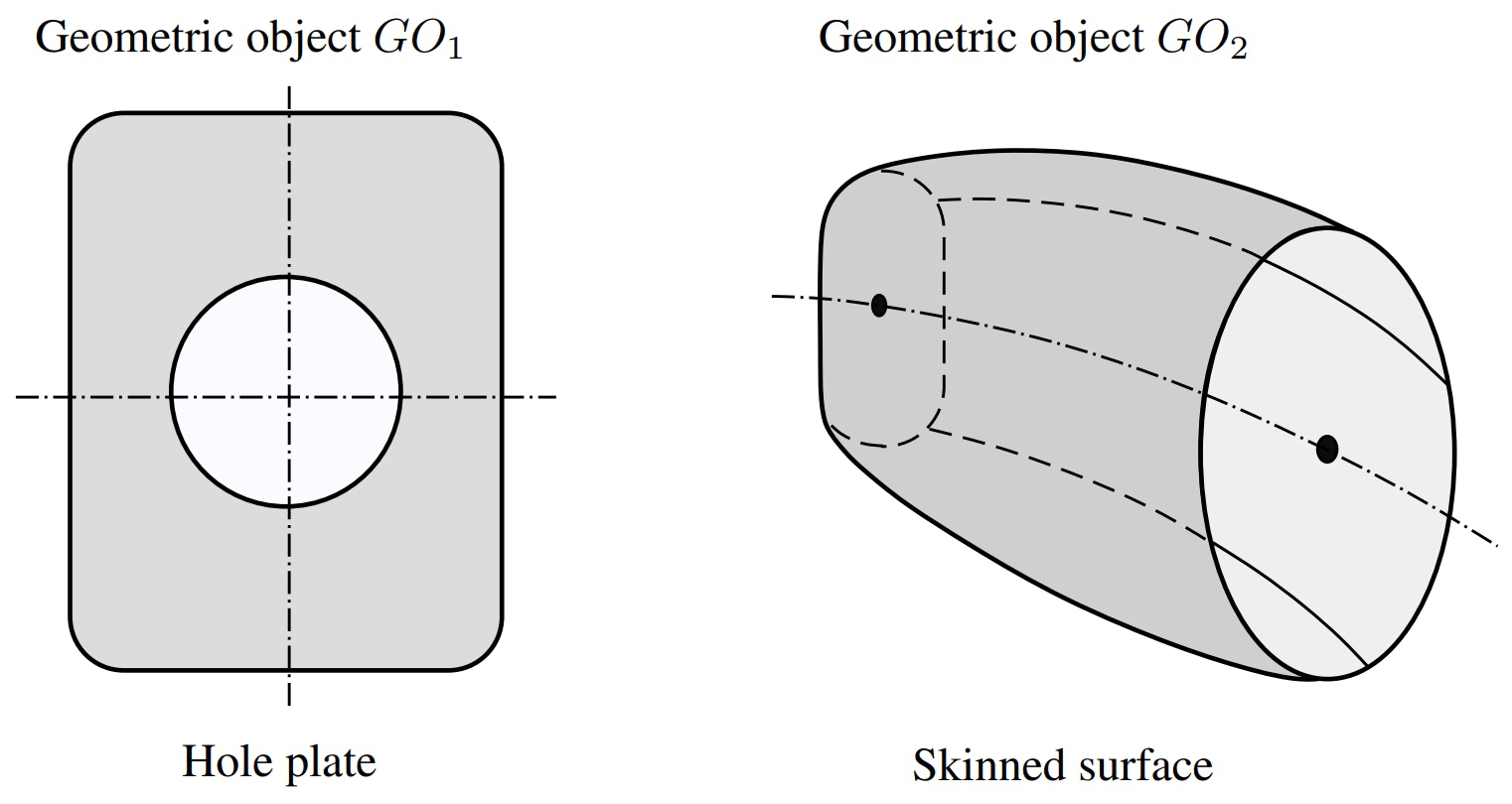
Here, both objects, GO1 and GO2, are built from the very beginning as discretized surfaces by using quadrilateral elements QEs (also called cells, panels, or boundary elements). Such simple geometrical elements were chosen because most of VLM- or PM-based codes rely on QE discretizations to represent the lifting and non-lifting surfaces. Next, we present a detailed description of how these objects are built through a discretized setting by using QE.
2.1.1 Object GO1
This kind of object consists of a rectangular plate together with a circular or ellipsoidal hole. In order to mesh it with QE we make use of the FG-squircular mapping1, which allows one to smoothly transform a circular domain into a square region parameterized as (Fernandez-Guasti, 1992). Knowing that 𝒟 and 𝒮 can be represented as a set of concentric circles and shrunken FG-squircles, we can establish a correspondence between the r disk and the 2r square region by mapping every circular contour in the interior of the disk to a squircular contour in the interior of the square (see Fig. 2).
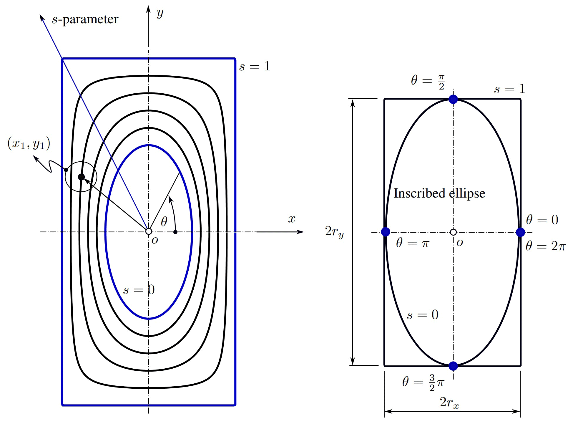
According to Fong (2021), an intermediate shape between a circle and a square can be represented by the following implicit equation:
where (x,y) is a set of Cartesian coordinates in ℝ2, s is the so-called squareness parameter which allows the shape to be interpolated between a circle and a square, and r is the radius of the original circle. While s=0 generates a circle of radius r, s=1 produces a square with a side length of 2r. In turn, Eq. (1) can be slightly modified to allow an ellipse to be smoothly transformed into a rectangle. Such a representation is given as follows:
When s=0, we obtain the equation of an ellipse with semi-axes rx, ry; when s=1 we obtain the equation for a rectangle with sides 2rx, 2ry. In order to facilitate the computation of intermediate shapes, Eq. (2) is recast in parametric form through mapping as
with , and provided that s≠0. On the one hand, when s=0, the shape corresponds to a circle or ellipse and therefore Eq. (3) reduces to the well-known parametric equation of a circle–ellipse. On the other hand, for θ∈Fθ, Eq. (3) becomes indeterminate and an alternative expression must be used. To avoid problems of a numerical nature, we define an interval around each element of Fθ, where TOL is the allowed tolerance. A deeper look at the FG-Squircular mapping allows us to recognize that, for given rx and ry, the values of θ∈Fθ generate points on both the rectangle and its inscribed ellipse (see Fig. 2). Therefore, we can again use the parametric equations of the ellipse to map Fθ.
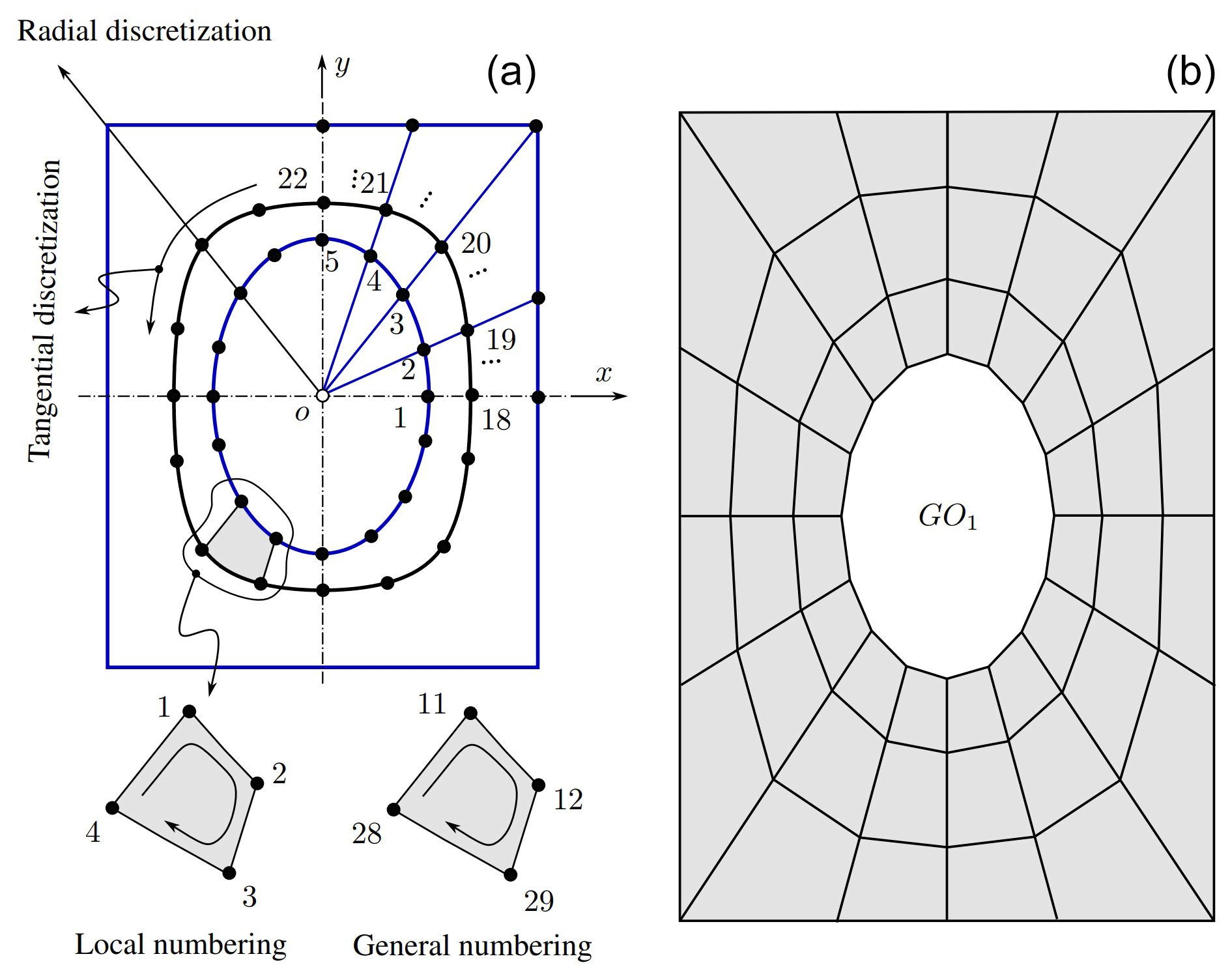
The object GO1 is geometrically decomposed into a finite set of quadrilateral cells as
where , Nr is the number of intermediate shapes (including both inner and outer contours), and Nc is the number of elements along their tangential direction. The total number of cells (or panels) is then given by the cardinal of E1, i.e., card(E1). In Fig. 3 (left) we present a schematic of how the division along the radial and tangential directions are performed. In Fig. 3 (right) we show the final mesh of a typical GO1 for Nr=4 and Nc=17, thus giving card(E1)=48 panels.
2.1.2 Object GO2
Surface generation in the context of computer-aided design (CAD) is typically done by using lofting or skinning processes. Although skinning can be understood as a sort of lofting (Ball, 1993), some differences have been introduced over the years. However, both processes are intended for passing a surface through a set of so-called cross-sectional curves. In this work, we adopted a specific skinning procedure, hereafter referred to as ruled skinning.
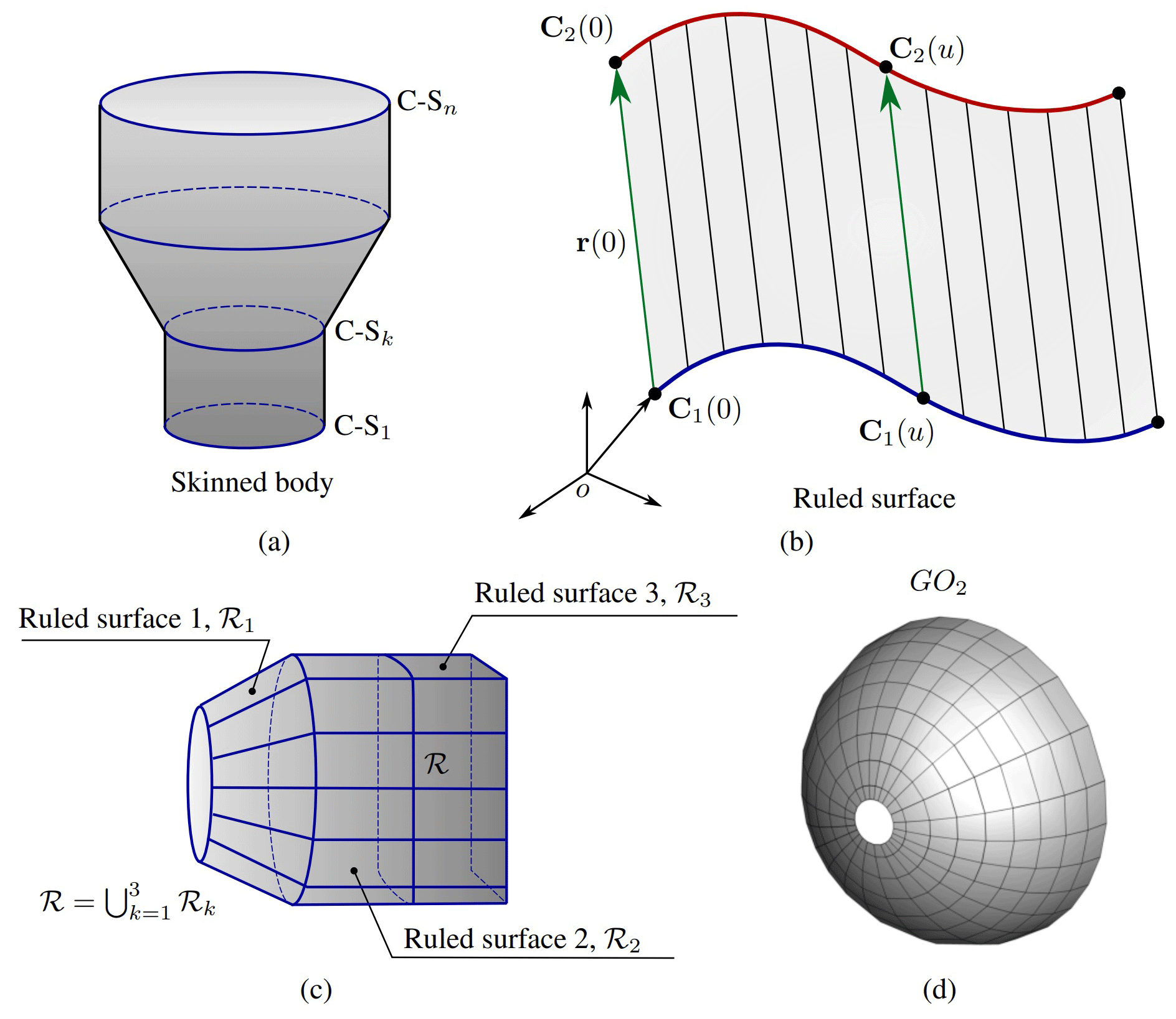
Figure 4(a) Skinned body (C-Sk stands for cross-section k), (b) ruled surface, (c) representation of a skinned body as a set of ruled surfaces, and (d) typical mesh of a GO2.
Ruled skinning provides the ability to skin a series of three or more profiles by placing ruled surfaces in between each section of profiles (see Fig. 4a). In turn, a ruled surface is defined by the property that through every point in the surface, there is at least one straight line which also lies in the surface. We can define a ruled surface more formally as a two-dimensional differentiable manifold constructed as the union of one parametric family of lines.
Definition 2.1: ruled surface
The following three definitions of a ruled surface are equivalent (Biran, 2019):
-
a surface such that through each point of it passes a straight line that is fully contained in the surface
-
a surface generated by the motion of a straight line
-
the set of a family of straight lines depending on a parameter that spans a set of real numbers.
Mathematically, a ruled surface can be described by
where is a parameterization for the curve 𝒞k⊂ℝ3. Any curve R(u0,v) with fixed parameter u0 is a generator line, the curve 𝒞k is a directrix of the representation, and the vectors r(u)≠0 describe the directions of the generators. Alternatively, we can generate a ruled surface by starting with two non-intersecting curves C1(u) and C2(u) as directrices and get the line directions as (see Fig. 4b).
In the context of wind turbines, some components (hub, nacelle, blades), although easily generated by a skinning process for modeling purposes, they cannot be represented by ruled surfaces. As an example, let us consider the surface ℛ shown in Fig. 4c. It is not a ruled surface if considered as a whole (first definition in Definition 2.1). However, ℛ can be obtained as the union of three ruled surfaces. Furthermore, every GO2 object is geometrically decomposed into a finite set of quadrilateral cells as follows:
where , Nrs is the number of ruled surfaces in what is decomposed, and E2,i is a finite subset of ℕ. Then, the total number of QE used to discretize is calculated as . In Fig. 4d we present the mesh of a typical hub nose, represented by Nrs=9 and , thus giving a total of 216 panels.
Finally, it should be stressed that any pair of cells belonging to GO1 or GO2 must meet the following requirements:
-
If Bk∩Bj for k≠j is exactly one point, then it is a common vertex (node) of Bk and Bj.
-
If Bk∩Bj for k≠j is a line, then it is a common facet of Bk and Bj (edge in two dimensions).
2.2 Wind turbine farm modeling
Here, we present a detailed description on how the surface of each component in a wind turbine farm is modeled in terms of the geometric objects already introduced in Sect. 2.1. Figure 5 provides a summary on which type of geometric object (GO1 or GO2) is involved in generating the discretized surface associated with each component of a wind turbine. From now on, we refer to mesh (or bound-vortex lattice) to make reference to a discretized surface.
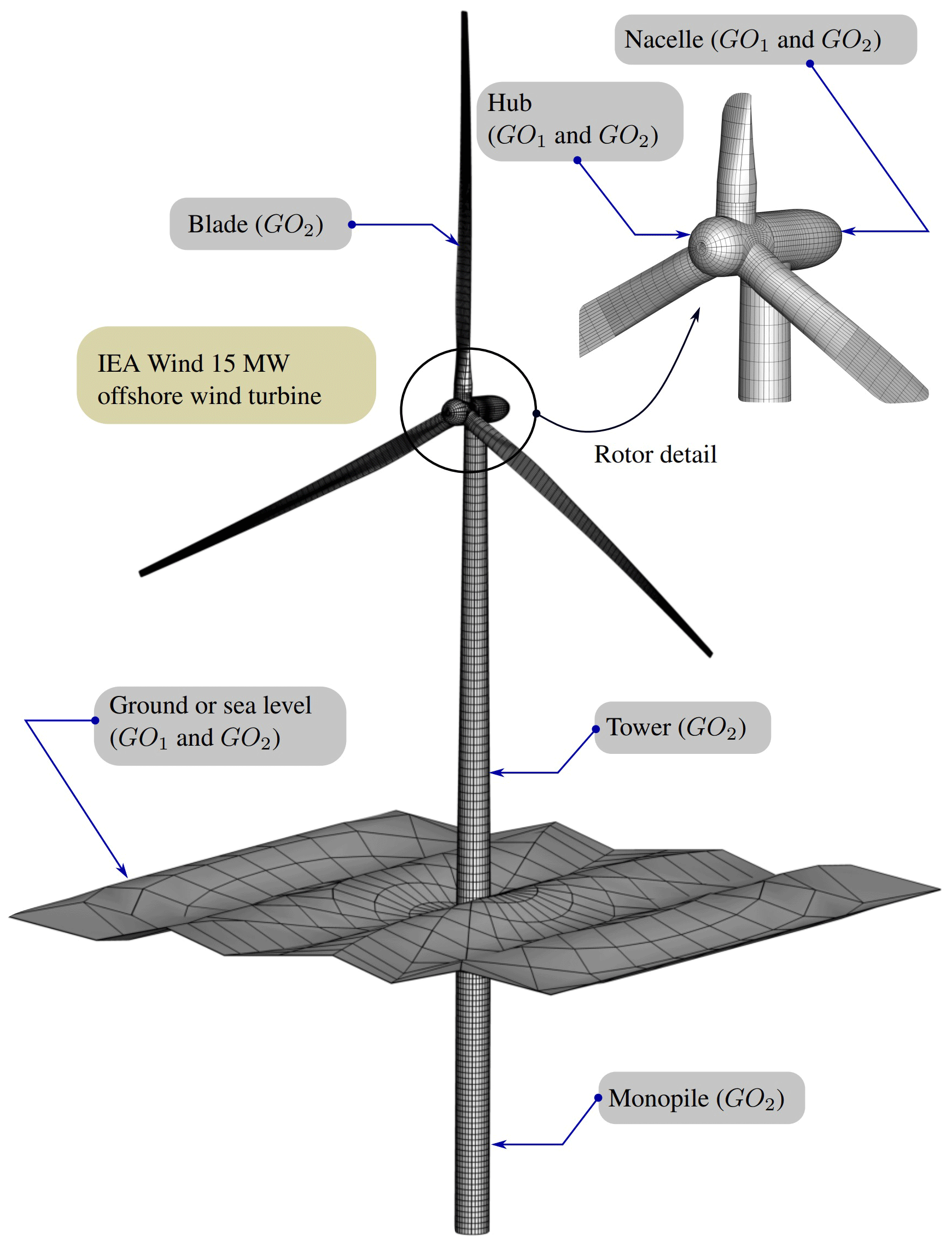
Figure 5Geometric modeling of a wind turbine: IEA Wind 15 MW offshore reference wind turbine.
Each wind turbine can be composed, at most, of six different components:
-
Blades are responsible for capturing part of the energy available in the wind.
-
The hub supports the blades and houses the pitch system.
-
The nacelle houses the components that convert mechanical energy into electrical energy.
-
The tower gives height to the rotor and supports the mass of the nacelle, hub, and blades.
-
The ground represents either the terrain for onshore wind turbines or the sea surface for offshore wind turbines.
-
The monopile holds the tower and the rest of wind turbine components above the sea floor.
The user can generate different wind turbine configurations by turning any of these components on or off. In the following subsections we will discuss in detail how to model each component and what parameters should be provided to generate them. All these parameters are specified through some options available in the main mesher script, as well as through a configuration ASCII file. This topic will be covered to some extent in Sect. 3 on computational implementation.
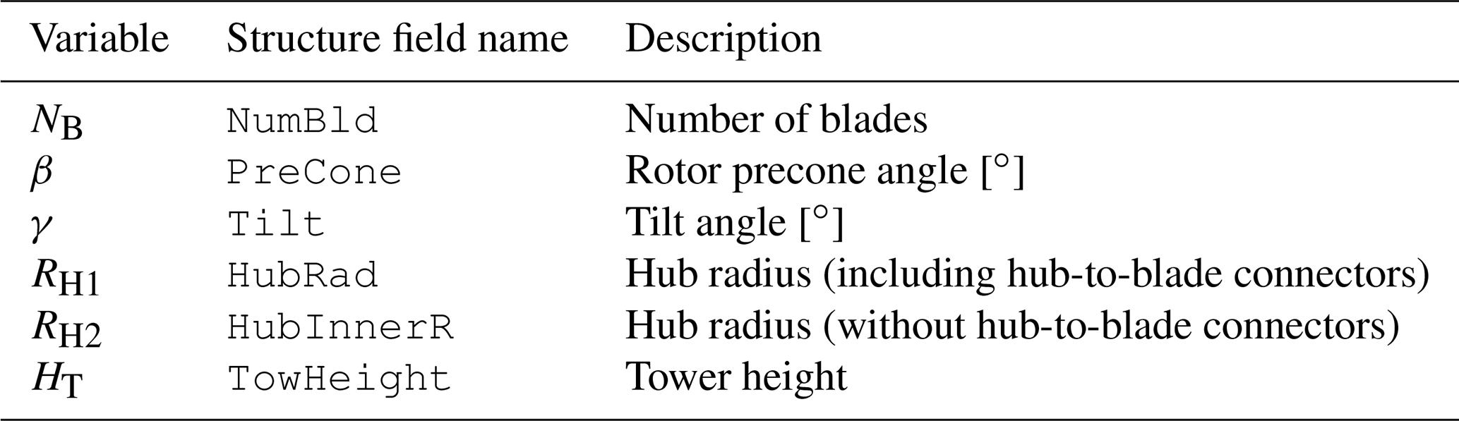
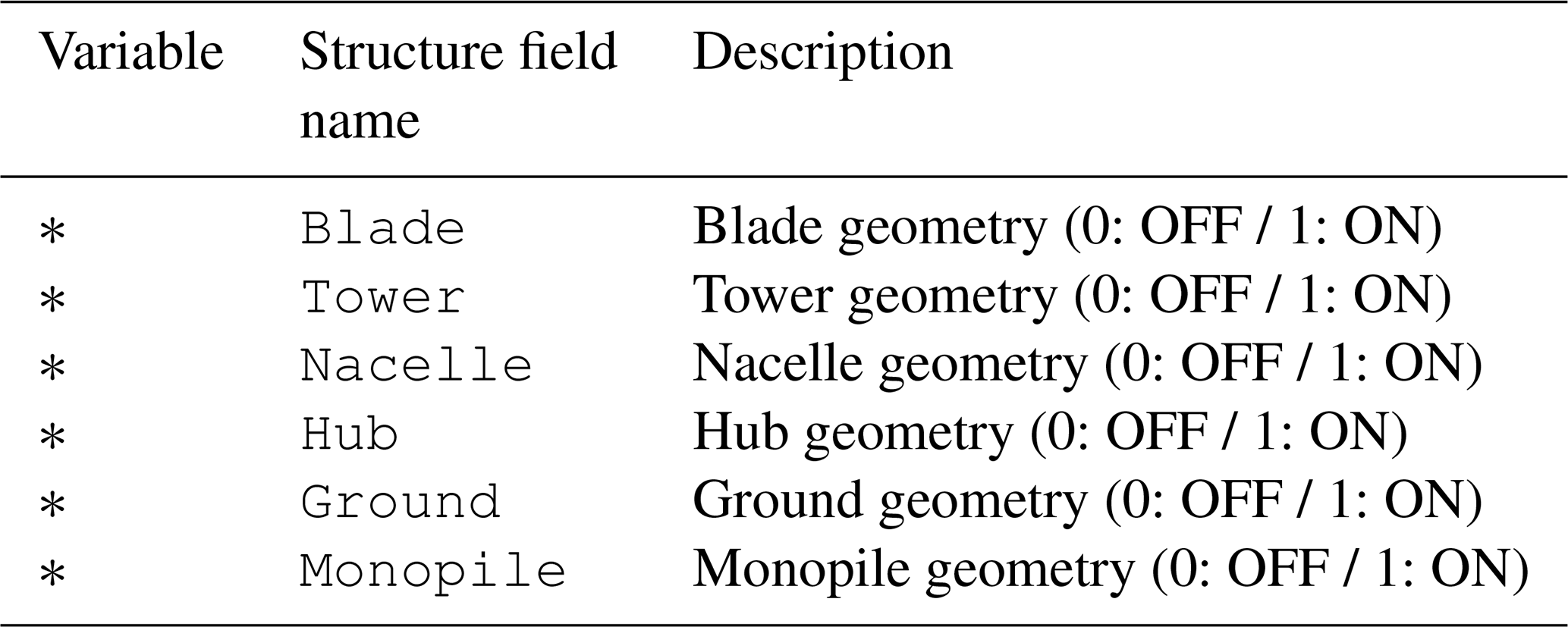
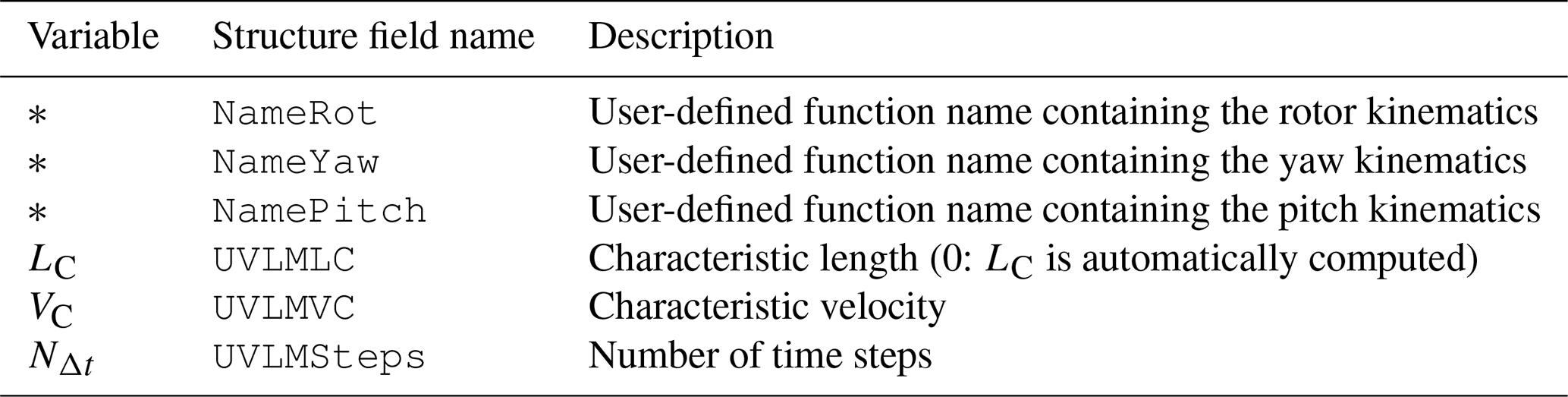
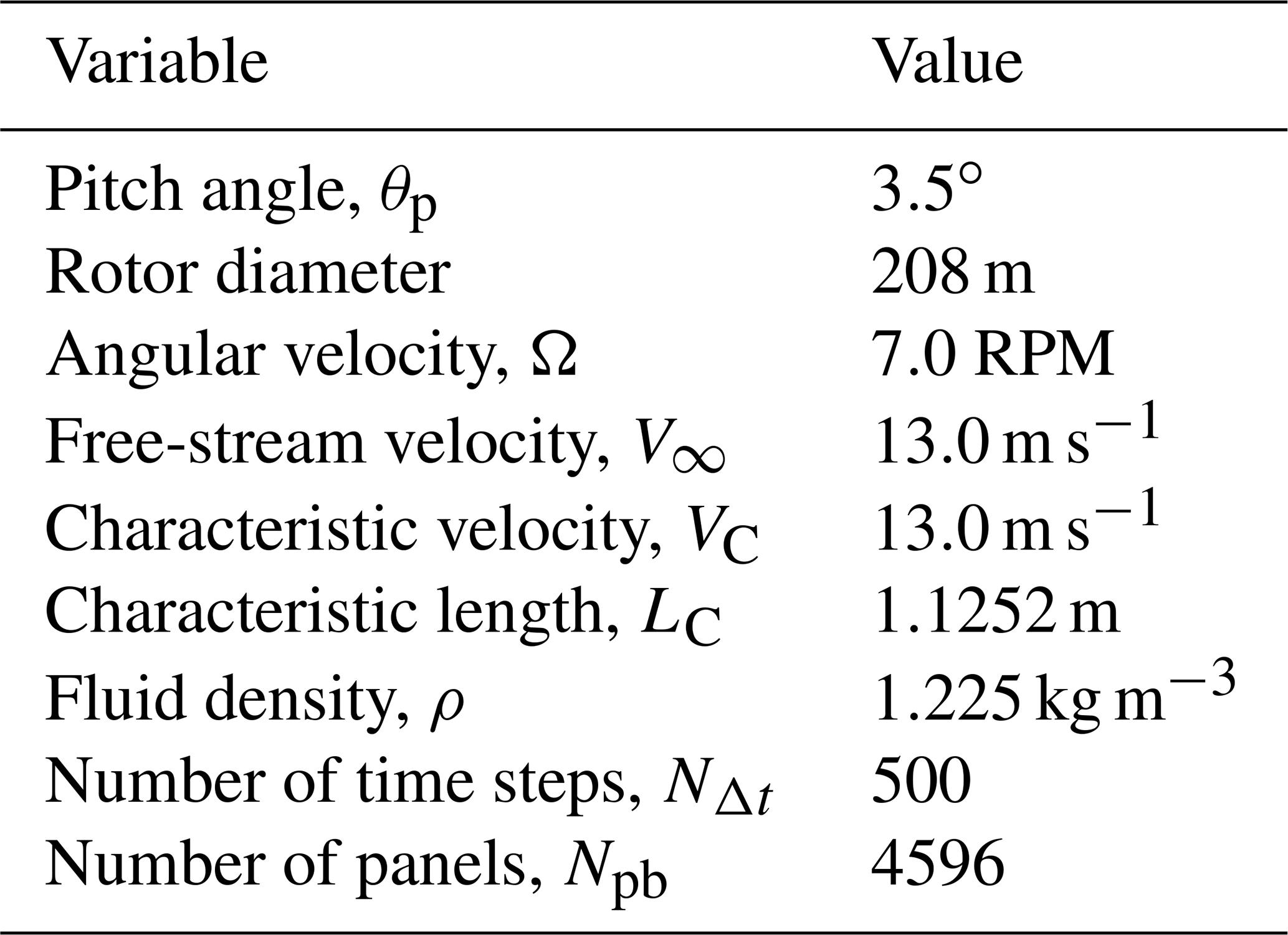
As usual, some of those parameters are related to the global configuration of the wind turbine; these are listed in Table 1. To complete the turbine setup, it is also required to indicate which components should be considered to build the wind turbine mesh (see Table 2).
Clearly, the number of blades cannot be increased indiscriminately. If this happens, there may be geometric interference between the hub surface and blade roots. Furthermore, as the number of blades is becoming larger and larger, it may happen that two blades are very close to each other, and therefore some geometrical interference may arise between them.
2.2.1 The tower and monopile
The tower and monopile components are essentially of the same kind. Both of them are ruled surfaces and therefore generated by GO2-like entities. As input data are necessary to generate the aerodynamic mesh associated with the tower and monopile, we need to provide the diameter at the ends of the component, its length, and number of aerodynamic nodes along its longitudinal and tangential directions. Tables A1 and A2 in Appendix A provide a summary of the variables associated with both components.
2.2.2 The nacelle
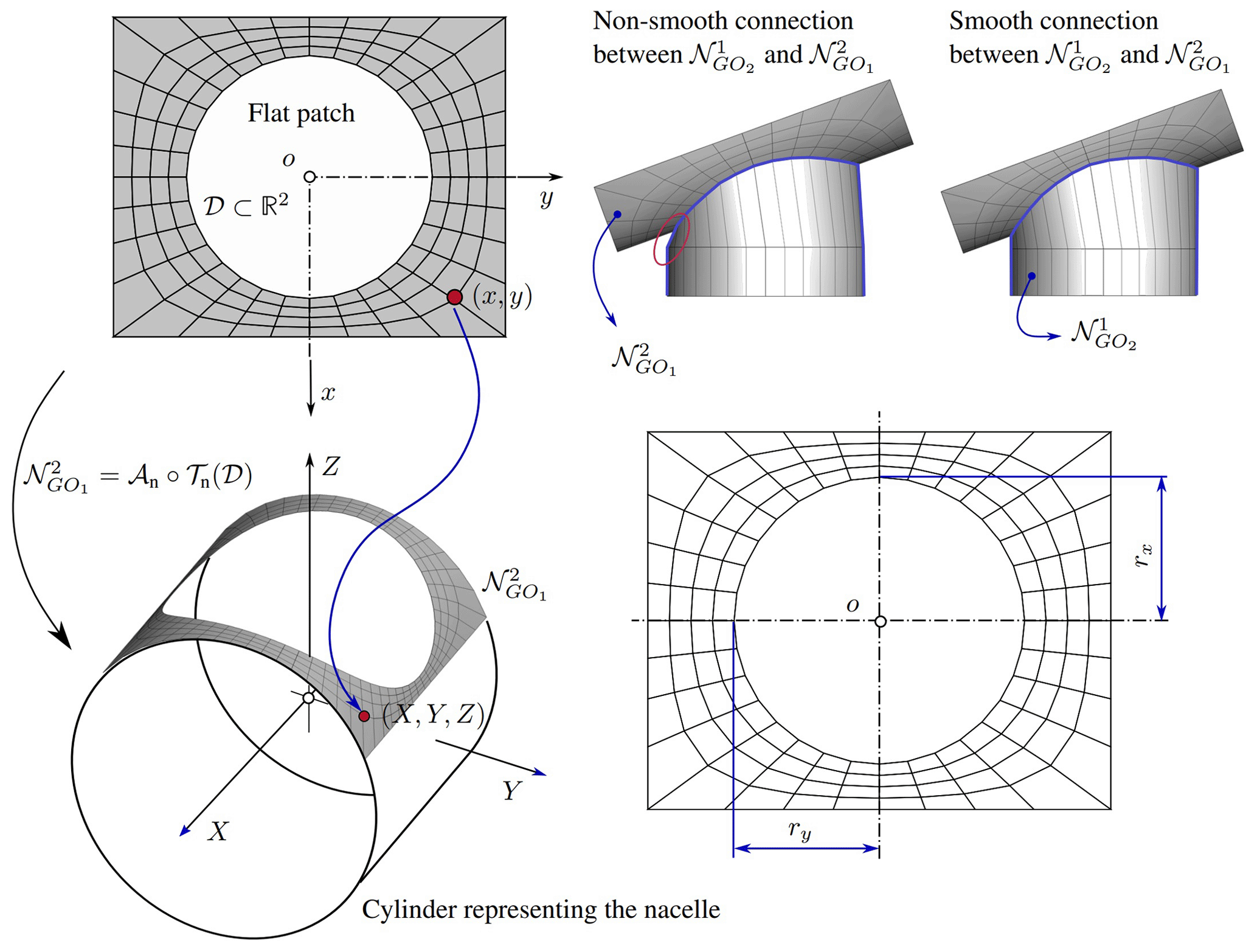
The aerodynamic mesh of the nacelle 𝒩 is generated as the union of four sub-meshes: (i) the tower–nacelle connector , (ii) a curved patch , (iii) a cylindrical surface , and iv) the tail of the nacelle . All nacelle components are generated by GO2-like entities with the exception of the curved patch, which is of type GO1. Figure 6 shows an exploded schematic of a typical nacelle of a wind turbine.
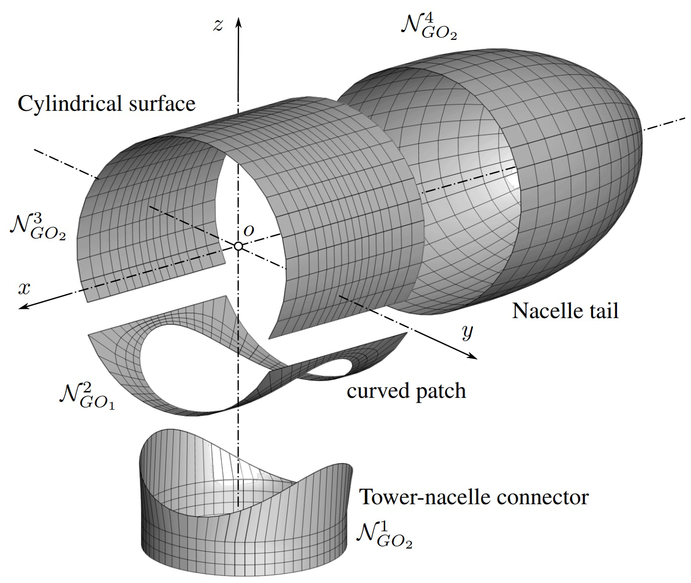
Among the several parameters involved in the design of wind turbines, the cone angle, tilt angle, and pitch angle are directly related with the aerodynamic behavior of the rotor. In particular, the tilt angle is used to provide sufficient clearance between the rotor blades and the tower. Here, for meshing purposes, such tilt angle γ is defined as the angle between the longitudinal axis of the nacelle and the horizontal plane. This definition implies that the nacelle axis is, in general, not orthogonal to the longitudinal axis of the tower and, therefore, not orthogonal to the axis of the tower–nacelle connecting piece either. In light of the above, the most complicated step to generate the aerodynamic mesh of the nacelle lies in the connection between the tower–nacelle connector and the nacelle itself, which is done through the curved patch . Such an object is obtained by following the next two steps in order:
-
Generate a typical flat GO1-like object with appropriate dimensions.
-
Deform it into a curved surface as shown in Fig. 6. In other words, it means rolling the patch over a “virtual” cylinder representing the nacelle (see Fig. 7).
For the second step, we consider a continuous deformation 𝒯n that maps each point r in a connected subset 𝒟⊂ℝ2 to a point R=𝒯n(r) on a surface in the three-dimensional space ℝ3. Mathematically, is given by
where RN1 is the radius of the cylinder representing the nacelle. It is straightforward to prove that the deformation map 𝒯n is an isometric map. Therefore, it preserves the length of every possible arc of material points on the parametric domain 𝒟. This is true if and only if the Jacobian D𝒯n on 𝒟 preserves the lengths of vectors in ℝ2 in the sense that for each r∈ℝ2. Equivalently, D𝒯n must obey , with I2 being the identity linear transformation on ℝ2 (Chen et al., 2018). Once the flat patch has been deformed into a curved patch, an affine transformation (translation and/or rotation) is applied to assemble it with the rest of the nacelle. Thereby, the object is obtained by means of the following map composition:
Finally, we need to address the non-smooth connection between the curved patch and the tower–nacelle connector. Such a non-smoothness arises as a consequence of two reasons: (i) the deformation of the original circular hollow cavity (flat patch) into an elliptical cavity (curved patch) and (ii) the misalignment between the tower longitudinal axis and the hollow axis of the curved patch. For this purpose, we compute in advance the radii of an elliptical hollow in the original flat patch that will ensure a smooth connection between the tower and the deformed curved patch (see Fig. 7). Such radii are given by
where RN3 is the tower–nacelle connector radius (see Table A3). When γ=0, the radius rx in Eq. (7) is directly the radius of the upper part of the tower (no tilt angle). However, the radius ry is different from the upper tower radius because of the deformation of the flat patch. Table A3 in Appendix A provides a summary of the variables associated with the nacelle.
2.2.3 The hub
The aerodynamic mesh of the hub ℋ is generated as the union of a series of sub-meshes depending on the number of blades of the wind turbine: (i) blade–hub connectors for , (ii) curved patches for , and (iii) the nose of the hub . All hub components are generated by GO2-like entities with the exception of the curved patches, which are of type GO1. Figure 8 shows an exploded schematic of a typical hub for a three-blade wind turbine.
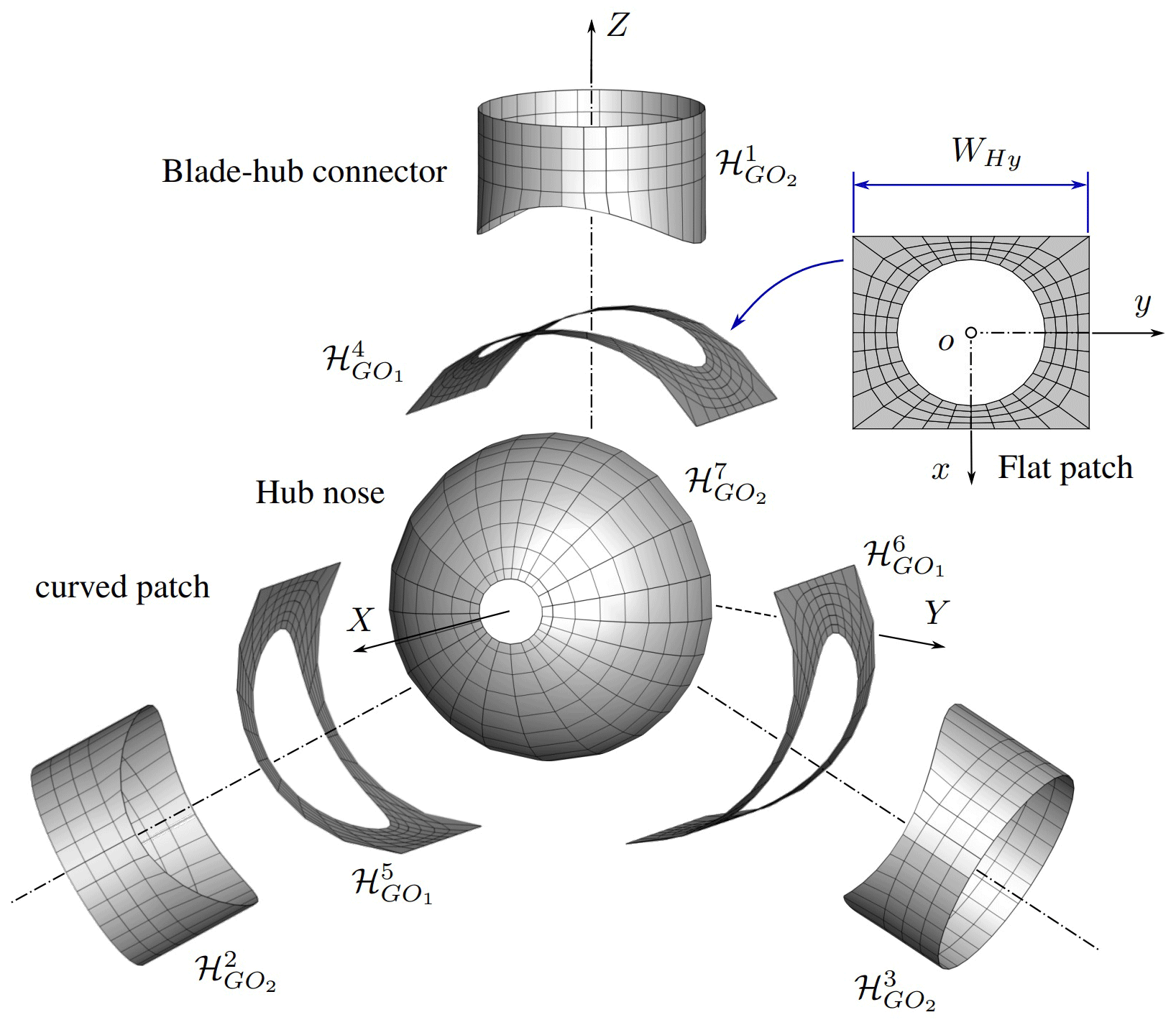
As before, the most complicated step to generate the aerodynamic mesh of the hub lies in the connection between the blade–hub connector and the hub itself, which is done through the curved patches. Those objects are generated by following a similar procedure as the nacelle:
-
Generate a typical flat GO1-like object with appropriate dimensions.
-
Deform it into a curved surface (see Fig. 7).
-
Make NB copies of this object and place them properly to assemble the rotor.
The deformation of a flat GO1-like object into a curved one resembling a part of the hub's surface is performed by means of a continuous isometric mapping as follows:
where RH2 is the radius of the cylinder representing the hub (without considering the blade–hub connectors). Once the flat patch has been deformed into a curved patch, we generated as many copies of the curved patch as the number of blades in the wind turbine. Then, an affine transformation for is applied to assemble each curved patch with the rest of the hub. Thereby, the object is obtained by means of the following map composition:
It should be noted that the dimension of the flat patches (before deformation) along the y coordinate (see Fig. 8) depends on the number of blades and the radius of the hub, i.e., . Finally, the radii of the elliptical hollow in the original flat patch that will ensure a smooth connection between the blade–connector and the deformed curved patch are given by
where β is the cone angle of the rotor, and RH3 is the blade–hub connector radius. When β=0, the radius rx in 11 is directly the radius of the blade–hub connector (no cone angle). Table A4 in Appendix A provides a summary of the variables associated with the hub.
2.2.4 The blade
The aerodynamic mesh of a blade ℬ is generated as the union of two sub-meshes: (i) the blade root and (ii) the lifting surface of the blade . All blade components are generated by GO2-like entities.
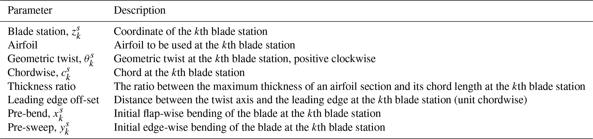
The mesh generation for wind turbine blades is a non-trivial process because it involves discretizing a three-dimensional surface whose shape changes along its longitudinal axis. Table 3 lists the geometric data that must be provided, as a function of the longitudinal coordinate, to build a three-dimensional wind turbine blade. To simplify what follows and avoid falling into excessive formalism, let us define B0 as the set of design parameters of the blade. Figure 9 presents an example of how such parameters are usually defined along the longitudinal axis of the blade. A good representation of its surface necessarily requires specifying these parameters at “several” points along the blade.
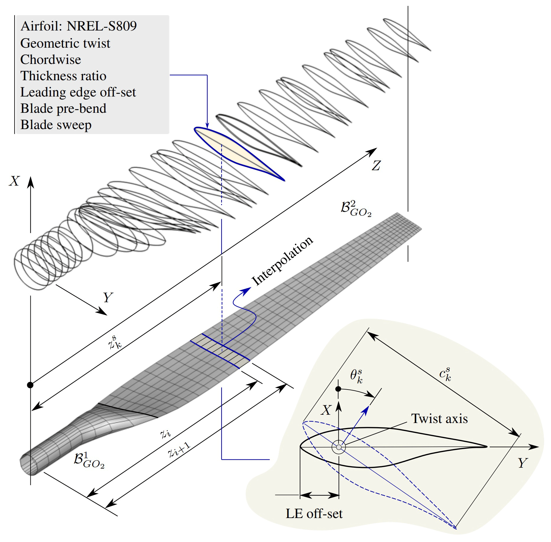
On this basis, the blade is divided into NB2−1 non-uniform intervals such that such that , where LB is length of the blade, z1=0, , and NB2 is the number of nodes along the blade (see Fig. 9). The geometric parameters at each coordinate zi are interpolated, according to the provided data B0, by using cubic splines. In the case of pre-bend and pre-sweep, we have two options, they are either provided by the manufacturer or they can be included by using Zuteck's formula (Larwood et al., 2014). The following equation is used to define the sweep and pre-bend:
where y and x are the local distance from the elastic axis (or pitch axis) to the sweep/pre-bend curve, ytip and xtip are the distance from the pitch axis to the sweep/pre-bend curve at the blade tip, z is the local distance along the blade measured from the blade root, z0 is the position of the beginning of the blade sweep/pre-bend, and ξ is the sweep/pre-bend exponent (see Fig. 10a). As mentioned above, the pre-bend and pre-sweep can be either automatically generated by using Zuteck's formula or manually specified by providing and at every station k.
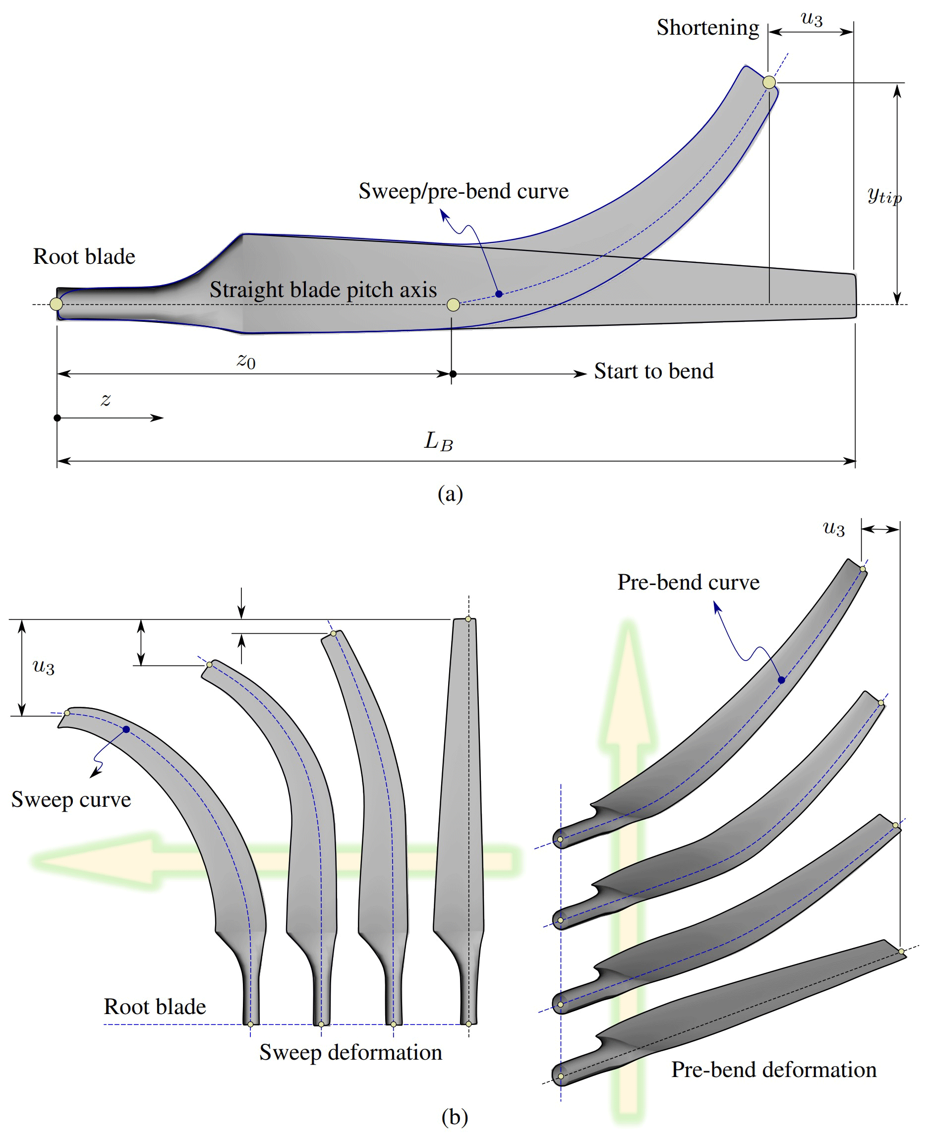
Figure 10(a) Parameters that define the wind turbine blade sweep and pre-bend and (b) sweep and pre-bend blade deformations.
The arc length for all curved blade shapes is equal to the original length of the straight blade, but with a slightly smaller rotor radius. The arc length of the blade should be kept the same to avoid blade extension, which will bias results towards longer blades that produce more power. To this end, we consider the position of an arbitrary point on the elastic axis of the blade at the reference configuration to be given by , while the position of the same point at the deformed configuration can be expressed as follows:
where u is the displacement vector. For a given coordinate z along the blade, the shortening in the axial direction, u3, due to the arc-length conservation can then be written as
where η is a dummy integration variable, s is the arc-length coordinate along the curved blade, and stands for derivative with respect to η. To obtain the shortening at a given blade section z (last expression in Eq. 14), we enforced the arc-length conservation by imposing that the length of the deformed blade must be equal to the original straight blade length, i.e., s(z)=z. The blade root is represented as z=0 in Eq. (14). The variables x and y represent the local distance from the pitch axis to the sweep and pre-bend curve, respectively. Then, the new nodal z coordinates associated with the initial partition [0,LB] are obtained as .
Once the new z coordinates are obtained, we perform a sanity analysis on all curved blades to check that the arc length is close enough to the length of the straight blade. Such an analysis is carried out by computing the difference between the original blade length and the curved blade length:
where zc is the tip radius of the curved blade. A script is used to automatically calculate zc, perform the arc length sanity check, and prepare the blade geometry. In Fig. 10b, we present some examples for sweep and pre-bend blade configurations. Table A5 in Appendix A provides a summary of the variables associated with the blade.
2.2.5 The ground
The aerodynamic mesh of the ground 𝒢 is generated using only a GO1-like object. As input data we need to provide (i) the ground–tower connection radius, (ii) the extent of the ground, namely, the side length of the square representing the ground area, and (iii) the number of aerodynamic nodes along its radial and tangential directions. Additionally, it is possible to generate an uneven ground by providing a user-defined function to compute the ground elevation or a scattered data set representing the ground elevation. The last option requires a fitting procedure (regression) to obtain the elevation on the ground aerodynamic mesh. This feature will be discussed in more detail in the computational implementation section. Table A6 in Appendix A provides a summary of the variables associated with the ground.
2.2.6 Wind turbine assembling
Once all the components for a given wind turbine configuration are generated, the next step is to assemble them to obtain the complete wind turbine mesh. The code internally calculates all the data required to assemble each turbine within the wind farm. The only information to be provided by the user is the initial rotor angle, the initial yaw angle, and initial pitch angles. Table 4 lists the data that must be supplied by the user to assemble the turbine. These data are located at the end of each turbine data sheet.
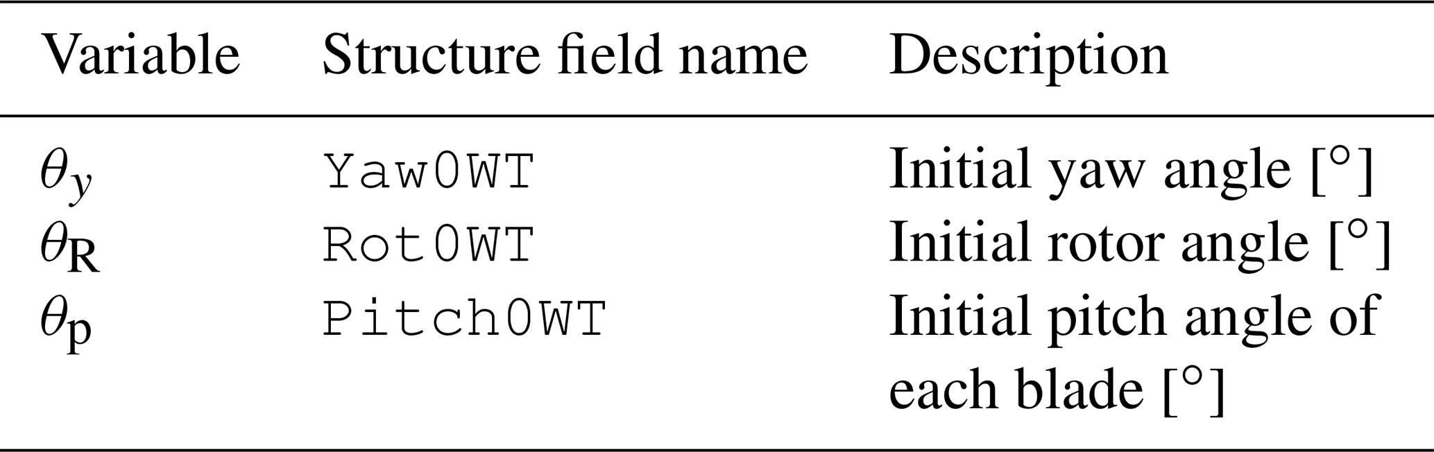
It should be stressed that the number of pitch angles to be provided must match the number of blades in the rotor, i.e., , and their values can be different from each other. As an example, we present below how the initial angles must be specified to configure a three-blade rotor.
0 % Yaw0WT - Initial yaw angle [degree]
0 % Rot0WT - Initial rotor angle [degree]
4,4,4 % Pitch0WT - Initial pitch angle [degree]
In this section we describe the main aspects associated with the computational implementation of the mesh generator code called UVLMeshGen developed at the University of Bergen (Norway) in collaboration with Universidad Nacional de Río Cuarto (Argentina). The full code is available in a GitHub repository (Roccia, 2023) for public access under a Creative Commons Attribution 4.0 International License.
This meshing tool is fully implemented in MATLAB®, and it is intended for generating meshes for onshore and offshore wind farms consisting of horizontal-axis wind turbines. Among the main features of UVLMeshGen, we can mention the following:
-
wind farm meshing,
-
terrain meshing,
-
specification of terrain topography,
-
kinematic processor, and
-
exporting files (Tecplot, UVLM, …).
UVLMeshGen provides meshing data into a series of structure variables by using typical FEM-oriented data arrays, such as nodal coordinate arrays and connectivity arrays. Next, we describe to some extent the organization of the code, description of the main script, important variables, and the features introduced above.
3.1 Code structure
The mesh generator is designed by following a procedural programming paradigm. The software contains two main blocks: (i) the geometric processor, which is responsible for generating the mesh of each wind turbine component and its assembling, and (ii) the kinematic processor, which is in charge for computing the kinematics of lifting and non-lifting surfaces. The exporting module, which is responsible for writing output files (Tecplot, input data for UVLM-based codes, etc.), can be added/modified by the user according to their needs. However, the code incorporates an option to export meshes in Tecplot format by default. In Fig. 11 we present a flowchart of UVLMeshGen.
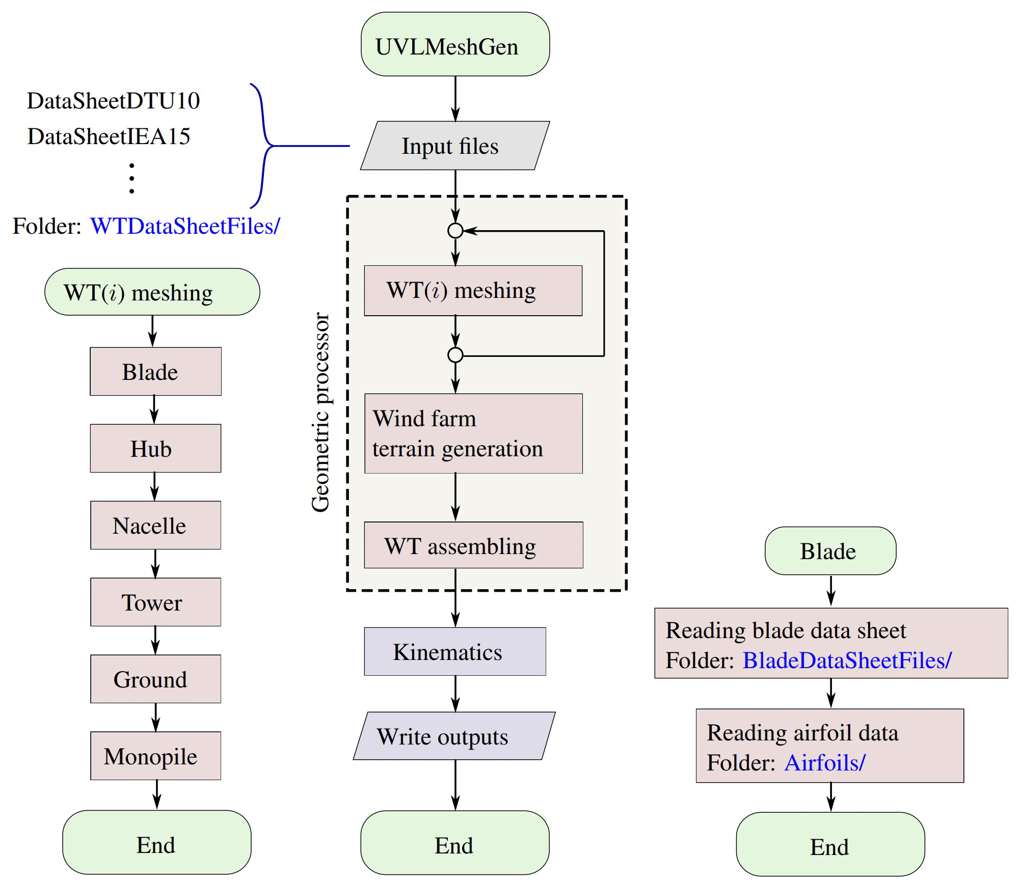
The input files needed by UVLMeshGen are ASCII files and user-defined MATLAB functions. To keep all the input files clean and separate from the main code, all of them are organized in several folders.
The code starts by loading as many input files as different wind turbines the wind farm contains. These files must be located inside the folder “WTDataSheetFiles/”, and they gather the geometric definition of each wind turbine. Then, the code generates the meshes associated with each wind turbine component. Among them, the blade requires an additional input file containing its complete setup (see Table 3), which must be located inside the folder “BladeDataSheetFiles/”. The blade configuration file also makes reference to the airfoil distribution along its spanwise direction, thus requiring further information about airfoil coordinates. These data are stored inside the folder “Airfoils/”.
Once all the components for each wind turbine have been generated, the code continues with the wind farm terrain, depending on whether it is activated or not in the main script. Then, all wind turbine parts are assembled to shape the final wind farm. The aforementioned processes, namely the generation of wind turbine components, terrain and their final assembly into a wind park, make up the so-called geometric processor.
UVLMeshGen also has a kinematics module that is in charge of generating pitch, yaw, and rotor motions. This module is general enough to allow any kinematics to be prescribed by the user through custom user-defined functions. Such a feature is very useful to investigate the aerodynamic performance of wind turbines. To write the outputs, users can either select some of the file formats included by default or provide their own scripts to export data.
3.2 Main script
The code is executed through a main script, which contains a set of general options, such as wind farm layout, terrain elevation, wind turbine kinematics, and output files. In Table 5 we present a brief description of the variables to be specified in the main script.
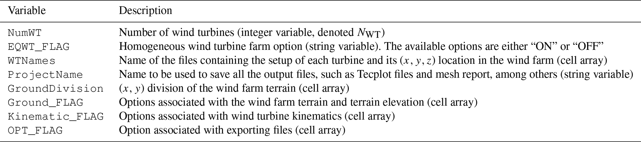
WTNames is a cell array variable of dimension NWT×4. The first column contains the file names associated with the configuration of each wind turbine in the wind farm. The last three columns contain the coordinates of each wind turbine. As an example, let us consider a wind farm made up of four different wind turbines (NWT=4). Under these assumptions, the variable WTNames could take the following values:
WTNames = {'DataSheet_DTU_10MW.DAT', 0.0, 0.0, 0.0
           'DataSheet_IEA_15MW.DAT', -100.0, 100.0, 0.0
           'DataSheet_Sandia01.DAT', -120.0, -120.0, 0.0
           'DataSheet_Sandia01.DAT',  100.0, -100.0, 0.0}.
EQWT_FLAG is a string variable which can take only two values: ON or OFF. If the value ON is used, the wind farm will consist of only one type of wind turbine. The setup of said turbine corresponds to the one specified in the first row of the variable WTNames. However the number of rows of WTNames must still be equal to the number of turbines considered in NumWT. This is because the wind turbines will be placed within the wind farm by extracting the coordinates from the variable WTNames.
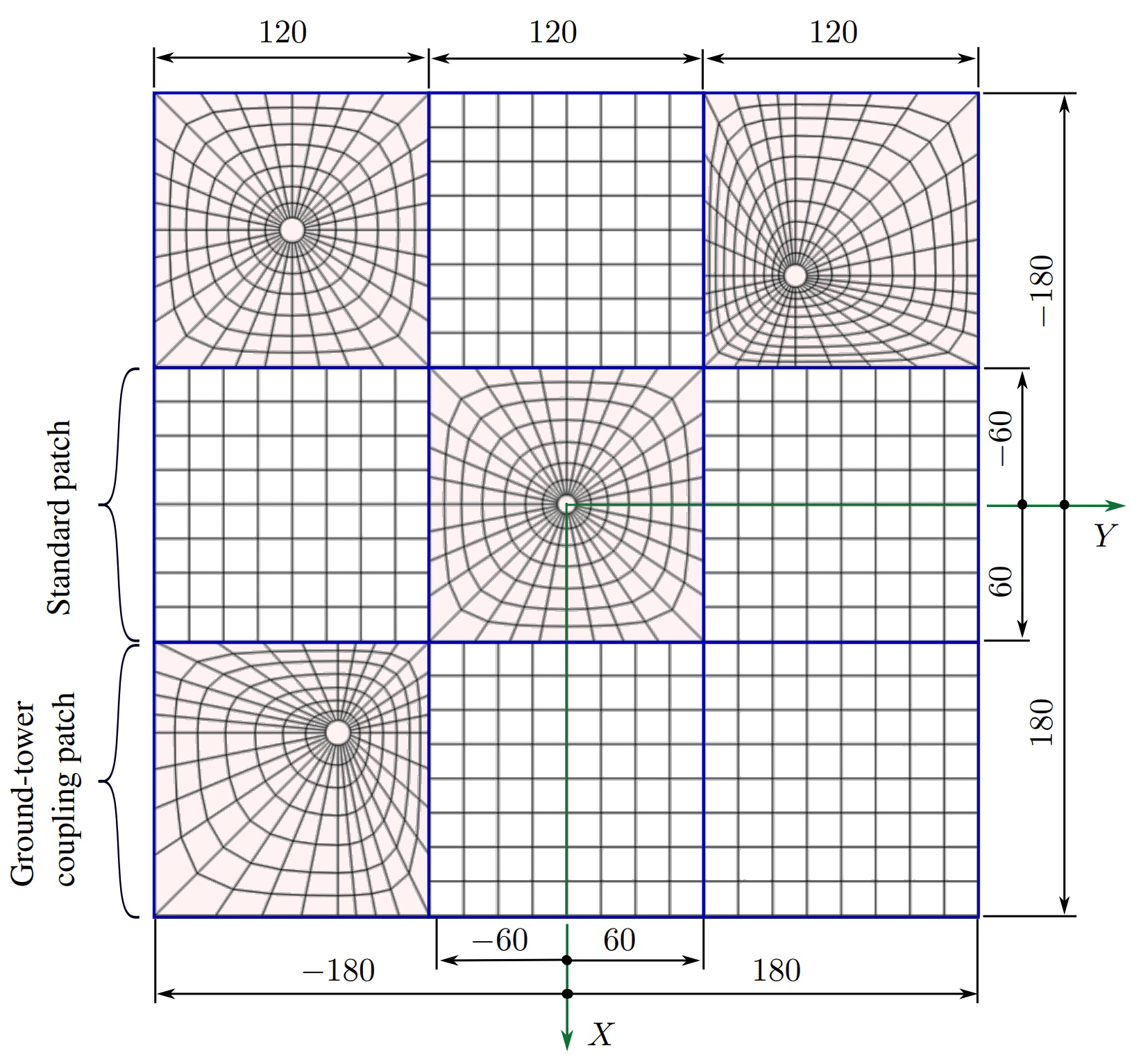
GroundDivision is a cell array variable of dimension 2×1. The cell 𝙶𝚛𝚘𝚞𝚗𝚍𝙳𝚒𝚟𝚒𝚜𝚒𝚘𝚗{1,1} contains the coordinates of the patches into which the terrain will be divided along the x direction. In a similar way, the cell 𝙶𝚛𝚘𝚞𝚗𝚍𝙳𝚒𝚟𝚒𝚜𝚒𝚘𝚗{2,1} contains the coordinates of the patches into which the terrain will be divided along the y direction. The number of patches along the x and y directions are determined as .
To ensure a smooth terrain surface with a regular discretization of elements, it is recommended to consider one patch per turbine in the wind farm. The dimensions of the patch must be large enough to accommodate the ground–tower coupling. Once the surface of the terrain is divided, the code will automatically determine where the turbines are located, it will generate the corresponding ground–tower coupling, and in those patches without turbines, the code will generate a rectangular grid. As an example, let us consider the wind farm introduced above (see variable WTNames). For this wind farm layout, a suitable terrain division could be as follows:
GroundDivision={[180, 60, -60, -180]
                [180, 60, -60, -180]},
from which it is clear that three patches were considered along both directions, i.e., nine patches in total. In Fig. 12 we present a schematic intended to explain how the terrain division is performed and the reference frame used.
Ground_FLAG is a cell array variable of dimension 1×6. All the cells contained in this array are of type string, and they specify whether or not to generate the wind farm terrain. In addition, this variable allows configuring the terrain elevation and what options will be used to generate it. The reader is referred to Sect. 3.4 for a more detailed description of this feature.
Kinematics_FLAG is a cell array variable of dimension 1×5. All the cells contained in this array are of type string, and they specify whether or not kinematics associated with different wind turbine components are generated (e.g., yaw motion, pitch motion, and/or rotor motion). Furthermore, this variable allows configuring the time step to be used for the kinematics when considering heterogeneous wind farms. The reader is referred to Sect. 3.5 for a more detailed description of this feature.
OPT_FLAG is a cell array variable of dimension 1×2. All the cells contained in this array are of type string, and they specify whether or not the generated meshing data will be exported. This option consists of two fields as follows:
OPT_FLAG={'ON','MyOutput'}, where the first cell supports two values {𝙾𝙽,𝙾𝙵𝙵}, which allow us to indicate whether the data coming from the meshing procedure should be exported or not, and the second cell specifies the name of the user-defined script to be used for exporting purposes. The code has built-in three export options by default: (i) TecplotOutput, which allows us to export the assembled wind farm in Tecplot format, (ii) TecplotKinematics, which allows us to export the assembled wind farm and its kinematics in Tecplot format, and (iii) VLMSim, which allows us to write the input files for the aerodynamic solver VLMSim (Vortex-Lattice Method – Simulation) developed by the Group of Applied Mathematics, Universidad Nacional de Río Cuarto (Verstraete et al., 2023). The second option requires the Kinematics_FLAG to be ON, otherwise an error will occur. All user-defined export scripts must be located inside the folder “Output Scripts/”.
3.3 Output data structure
When UVLMeshGen is executed, it will generate four main structure variables where all meshing data are stored. These variables are WIND_TURBINE, CONNECT, GROUND_FARM, and KINEMATICS. The first variable contains only data associated with mesh coordinates and geometric dimensions related to the entire wind farm. The second structure variable contains all connectivity arrays associated with the entire wind farm discretization. The third variable contains the wind farm kinematics, namely, positions and velocities of the entire wind farm mesh for the stipulated simulation time grid. The last variable contains all data associated with the wind farm terrain.
-
The
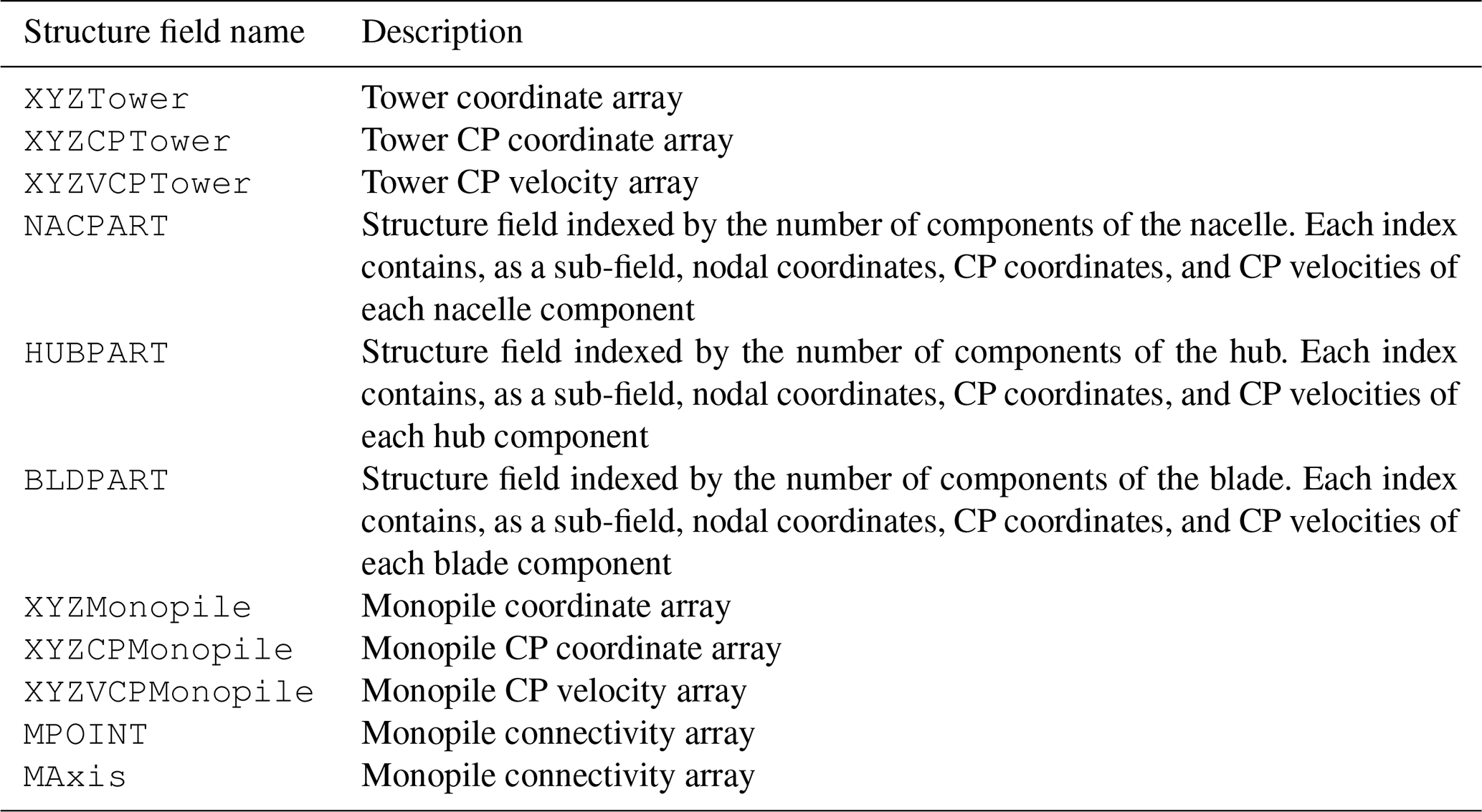
WIND_TURBINEvariable is indexed by the number of wind turbines within the wind park, i.e.,WIND_TURBINE(i)for . In Table B1 in Appendix B, we list the main fields associated withWIND_TURBINEstructure. If any component of the wind turbine is disabled during the geometric modeling, the field associated with it is assigned the “empty value”. -
As before, the
CONNECTvariable is indexed by the number of wind turbine within the wind park. In Table B2 in Appendix B, we list the main fields associated withCONNECTstructure. -
The
GROUND_FARMvariable contains only information regarding the wind farm terrain. There is no kinematics associated with the terrain since it is motionless, so its position is the same over time, and therefore the velocities at the control points are zero for all t. In Table B3 in Appendix B, we list the main fields associated withGROUND_FARMstructure. The fieldGROUND_FARM.PATCH(i)for , where NGp is the number of patches into which the terrain was divided, contains nodal coordinates and connectivities, among other data. -
The
KINEMATICSvariable is indexed by the number of simulation time steps used by the kinematics processor, i.e.,KINEMATICS(i)for , where NΔt is the number of time steps. As fields, this variable contains (i)KINEMATICS(i).GroundFarm.PATCH(k)for and (ii)KINEMATICS(i).WT(j)for . Although the terrain is motionless,KINEMATICS(i).GroundFarmstores the nodal coordinates, control point (CP) coordinates, and CP velocities (which are zero) over time. This decision on the storage of terrain data is based on a potential future implementation of “terrain motion” to simulate the sea surface and the effects of waves on offshore wind turbines. The fields associated with the second structure,KINEMATICS(i).WT(j), are listed in Table B4 in Appendix B.
3.4 Wind farm terrain processor
This module is in charge of generating the wind farm terrain. All necessary parameters are introduced via the Ground_FLAG cell array variable located in the main script. As previously mentioned, this variable consists of six cells as follows:
Ground_FLAG={'ON','ON','userfunction','MyGround',
'GroundData.DAT','poly23'},
where the first and second cells admit two values {𝙾𝙽,𝙾𝙵𝙵} indicating whether the wind farm terrain generation is activated or not and whether the terrain elevation feature is enabled or not, respectively. The third cell supports two different keywords {'𝚞𝚜𝚎𝚛𝚏𝚞𝚗𝚌𝚝𝚒𝚘𝚗','𝚎𝚡𝚝𝚎𝚛𝚗𝚊𝚕𝚍𝚊𝚝𝚊'}, which specify whether the terrain elevation will be generated via some user-defined function or whether it will be generated by fitting a scattered terrain data set. The fourth and fifth cells specify the name of the user-defined function and the name of the file containing the terrain data set, which should be placed inside the “Terrain Data/” folder. The mesher will use either the function or the data set according to the option specified in the third cell. The last cell specifies the fit type to use if externaldata is selected. Internally, the mesher uses the MATLAB® intrinsic function “fit” to fit a surface to the data provided by the external file. Any fitting option accepted by fit can be specified as a valid option in Ground_FLAG.
The user-defined function for generating the terrain elevation must receive two inputs: (i) an array of dimension NWF×3 (where WF denotes wind farm) containing the nodal coordinates of the flat wind farm terrain and (ii) the number of nodes of the wind farm terrain, NWF. The terrain coordinates within the input array are organized as follows: x coordinates (first column), y coordinates (second column), and z coordinates (third column). The user can impose/calculate any elevation profile on the ground (coordinates z) as long as it does not present abrupt changes. As output, the function only needs to provide an array of coordinates of dimension NWF×3, where the third column contains the z coordinates modified according to the elevation model proposed by the user. As an example, we provide below a very simple user-defined function that allows us to impose a terrain elevation profile.
function C = MyTerrainLevel (XYZ, NWF)}}
Ymin = min(XYZ(:,2));
Ymax = max(XYZ(:,2));
DD   = Ymax - Ymin;
C = XYZ;

A = [Ymin^2 Ymin 1; Ymax^2 Ymax 1; 2*Ymin 1 0];
F = [0; DD/6; 0];
Coef = A\textbackslash F;

for i = 1:NWF
 C(i,3) = Coef(1)*C(i,2)^2 + Coef(2)*C(i,2)^2 + Coef(3);
end
Figure 13 shows the elevation of the ground surface generated by using a parabolic and a sinusoidal profile. The ground surface corresponding to the parabolic profile was generated using the user-defined function introduced above. As can be seen, the elevation profile does not present any type of abrupt changes or jumps.
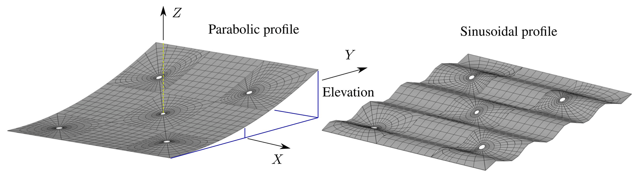
When the option 'externaldata' is chosen, an external ASCII file containing coordinates of points on the ground must be provided. The amount/quality of the points considered should be large/good enough to ensure that the fitted surface renders a realistic elevation profile. Once the fitting process is done, the resulting surface equation will be used to find the elevation for a given nodal terrain coordinate (x,y). The data must be provided in three columns: x coordinates (first column), y coordinates (second column), and z coordinates (third column).
3.5 Kinematic processor
This module is in charge of generating the kinematics for the entire wind farm. As before, all necessary parameters are introduced via the Kinematic_FLAG cell array variable located in the main script. As previously mentioned, this variable consists of five cells as follows:
Kinematic_FLAG={'ON','RotorOFF','YawOFF','PitchOFF','min'},where the first cell admits two values {'𝙾𝙽','𝙾𝙵𝙵'} indicating whether the wind farm kinematics is enabled or not. The second through fourth cells allow us to specify whether rotor, yaw, and pitch kinematics are enabled or not. Each of the following cells admits two values: {'𝚁𝚘𝚝𝚘𝚛𝙾𝙽','𝚁𝚘𝚝𝚘𝚛𝙾𝙵𝙵'}, {'𝚈𝚊𝚠𝙾𝙽','𝚈𝚊𝚠𝙾𝙵𝙵'}, and {'𝙿𝚒𝚝𝚌𝚑𝙾𝙽','𝙿𝚒𝚝𝚌𝚑𝙾𝙵𝙵'}.
When considering a wind farm, it may happen that it is composed of different types of turbines (heterogeneous wind farm), which can in turn result in very different aerodynamic grids (e.g., large differences in the size of aerodynamic panels). In UVLM-based codes it is customary to define characteristic magnitudes for computing force coefficients. Typically they are the characteristic density ρC, the characteristic length LC, the characteristic velocity VC, and the characteristic time TC, which is obtained as . UVLMeshGen offers two options for setting the characteristic length. This can be either provided by the user or computed by using a default internal procedure. If the automatic option is selected, LC is calculated based only on the discretization of the blade lifting surface as follows:
where NLS is the number of panels on the blade lifting surface, and Ai is the surface area of the ith panel belonging to the lifting surface. Regarding the characteristic velocity, it is usually set to be the magnitude of the free-stream velocity, i.e., VC=V∞.
Under the above definitions, it is clear that the time step used by standard UVLM codes based on time-stepping schemes directly depends on the spatial discretization of the blade, i.e., how fine or coarse the aerodynamic grid is. This fact is particularly important for generating the kinematics of heterogeneous wind farms. In a scenario like this, each wind turbine will have its own time step, which greatly complicates the aerodynamic simulation of the wind farm. A simple way to overcome this problem is to define an unique time step for the entire wind farm, Δtwf. Clearly, there are several ways to define such Δtwf: (i) a minimum time step, (ii) a maximum time step, or (iii) an average among the time steps associated with different wind turbines. These three options are available in UVLMeshGen by specifying 'min', 'max', or 'average' in the last cell of Kinematic_FLAG. According to the option selected, Δtwf is computed as follows:
where Δti is the time step associated with each wind turbine in the farm. In Table 6, we provide a summary of further kinematic variables that must be specified in each wind turbine sheet file (variable WTNames described in Sect. 3.2).
User-defined functions must be placed inside the “Kinematic Files/” folder. The mesher will use such M-Files functions to generate the kinematic laws for rotor, yaw, and pitch depending on whether such options are enabled in Kinematic_FLAG or not. Each of these functions must receive three inputs: (i) number of time steps, (ii) time step, and (iii) initial angle. For functions related to the rotor and yaw kinematics, the third argument is a scalar variable that specifies their initial angles. In the case of pitching, such a variable is a vector of dimension NB containing the initial pitch of each blade in the rotor. As output, the function must provide two arrays of dimension: 1×NΔt for rotor and yaw kinematics and NB×NΔt for pitch kinematics. The first output variable contains the angle time series, and the second one contains the time derivative of the angle time series. As an example, we provide below a very simple user-defined function which allows us to impose a harmonic yaw motion on a rotor wind turbine.
function [A, DA] = MyYaw (NTS, DT, A0)
A0 = A0 * pi / 180;
YH = 60 * pi / 180;
YW = 0.35;
T = linspace(0,NTS*DT,NTS+1);

A = A0 + YH * sin (YW * T);
DA = YH * YW * cos (YW * T);
It should be noted that all input angles are in degrees.
In this section, we present a series of results to show the capabilities of the mesh generator developed here to build arbitrary wind turbines and wind farm UVLM meshes. To this end, we use the UVLMeshGen along with the VLMSim to reproduce several standard results in the field of wind energy. Furthermore, we present some numerical simulations related to well-established wind turbine concepts such as the Sandia 100 m 13.2 MW wind turbine SNL100-00 and the DTU 10 MW reference wind turbine. Finally, we show the versatility and potential of the mesher through the generation of two different entire wind farms. Additionally, without falling into quantitative aspects about the aerodynamic loads generated on the blades, we present some qualitative snapshots of the wakes emanating from the wind park by using the method described in Appendix C.
All study cases presented in this work, the VLMSim solver was run on a desktop computer with an Intel(R) Core(TM) i7-8700 CPU at 3.20 GHz with 16 GB of RAM memory.
4.1 Solidity study
The rotor solidity is a dimensionless number commonly used for designing rotors, such as rotorcraft, propellers, and wind turbines. This is function of the aspect ratio and number of blades in the rotor thus providing a measure of how close a lifting rotor system is to an ideal actuator disk in momentum theory. Rotor solidity σ is defined as the fraction of the annular area in the control volume which is covered by the blades, i.e.,
where c(r) is the local chord and r is the radial position of the annular control area.
To analyze the influence of rotor solidity on the power output of a wind turbine, we consider 10 different configurations, where the number of blades is varied from 1 to 10. We select a blade similar to the SNL100-00 wind turbine. The rest of the parameters are as follows: air density ρ=1.29 kg m−3, free-stream velocity V∞=13.0 m s−1, wind turbine radius R=110 m, angular velocity Ωr=7.44 RPM, pitch angle , and rotor swept area Ar=πR2. The blade was discretized into 10 elements along the chord and 40 elements along the span. The characteristic length and velocity are LC=2 m and VC=V∞ respectively, which in turn gives a time step s. The rest of the simulation parameters are number of time steps NΔt=500, bound-vortex-lattice cut-off δc=0.01, and wake cut-off δc=0.01 (see Appendix C). Using such parameters, the wake length obtained for all rotors considered in this subsection is approximately 4.5 times the wind turbine rotor diameter.
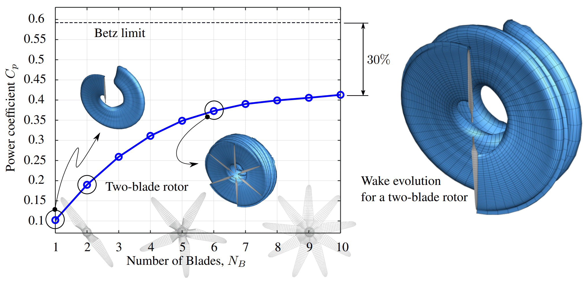
As a reference power, we select the wind power crossing the rotor area, i.e.,
which allows us to introduce the power coefficient as . Figure 14 depicts the Cp as a function of the number of blades. VLMSim predicts a solution that is in complete agreement with theoretical results. The study shows that power coefficient increases rapidly at first with the number of blades. Although the power continues to grow, the curve presents a very noticeable asymptotic behavior for 10 blades. Such a trend exhibits a difference of approximately 30 % with respect to the well-known Betz limit for 10 blades. Let us remember that it establishes a theoretical limit for the power that can be extracted from the wind (), so that such a difference of around 30 % can be associated with a number of factors, such as finite number of blades, blade geometry, non-optimal rotor configuration, etc. In practice real wind rotors have maximum Cp values in the range of 25 %–45 % (Bedon et al., 2012).
4.2 Yaw study
Another key factor associated with the power extraction from the wind is the yaw angle of the wind turbine with respect to the free-stream velocity. Rotor yaw reduces the effective projected area exposed to wind flow, thus reducing the energy conversion efficiency of the turbine. Yaw occurs when the wind direction is not perpendicular to the rotor plane. As a consequence, the blade will experience a varying relative velocity and angle of attack, leading to even more unsteady aerodynamics phenomena.
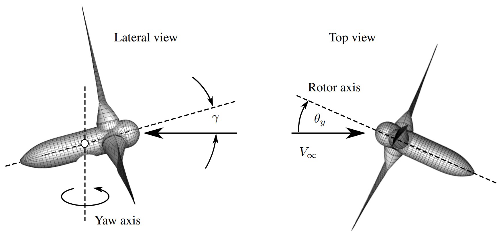
It is clear that the effective velocity of the wind to be considered to estimated the output power of a yawed rotor is its projection on the rotor axis (see Fig. 15) (Gebhardt, 2012), which can be expressed as
where the tilt angle γ was previously introduced, and θy is the yaw angle measured in a plane normal to the vertical (see Fig. 15). In addition, the output power of a wind turbine can be expressed as a function of the aerodynamic torque and the rotor angular velocity as follows:
where is the effective dynamic pressure, LC is some characteristic length (e.g., LC in Table 6), CM is aerodynamic moment coefficient, and Ω the rotor angular velocity. Introducing Eq. (20) into Eq. (21) and dividing by the power at , we get the following expression for a normalized output power:
where the ratio is a nonlinear function of θy. However, it approaches unity for small values of yaw angle. Therefore, as a first approximation, it can be considered that the ratio behaves like the function cos 2θy.
To analyze the influence of yawed rotors on the power output of a wind turbine, we consider different values of θy ranging from −60 to 60∘. For this study, we selected the SNL100-00 wind turbine operating under the same working conditions and spatial/temporal discretizations as in Sect. 4.1. The resulting output power is then normalized with respect to the power at .
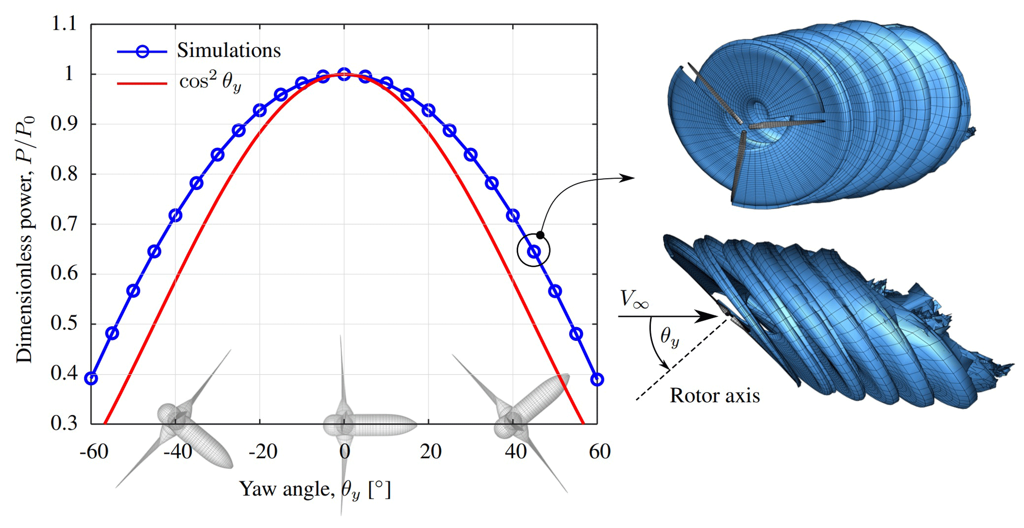
In Fig. 16 we show how the yaw angle affects the normalized output power. For angles lower than 15∘, the power practically behaves as the function cos 2θy; i.e., nonlinearities associated with CM(θy) are small. Beyond 15∘, simulations diverge significantly from the function cos 2θy, thus meaning that nonlinearities become important.
4.3 Pitch study
One of the main control parameters in wind turbines is the pitch angle θp, which allows us to regulate the output power according to the environmental conditions. For flow velocities less than the rated wind speed, the blade pitch is modified in order to maximize the output power. Similarly, for flow velocities beyond the rated wind speed, the blade pitch is also modified in order to avoid excessive angular speeds or runaway events.
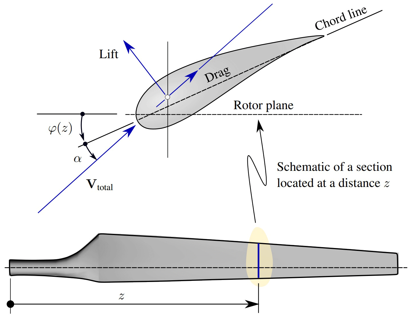
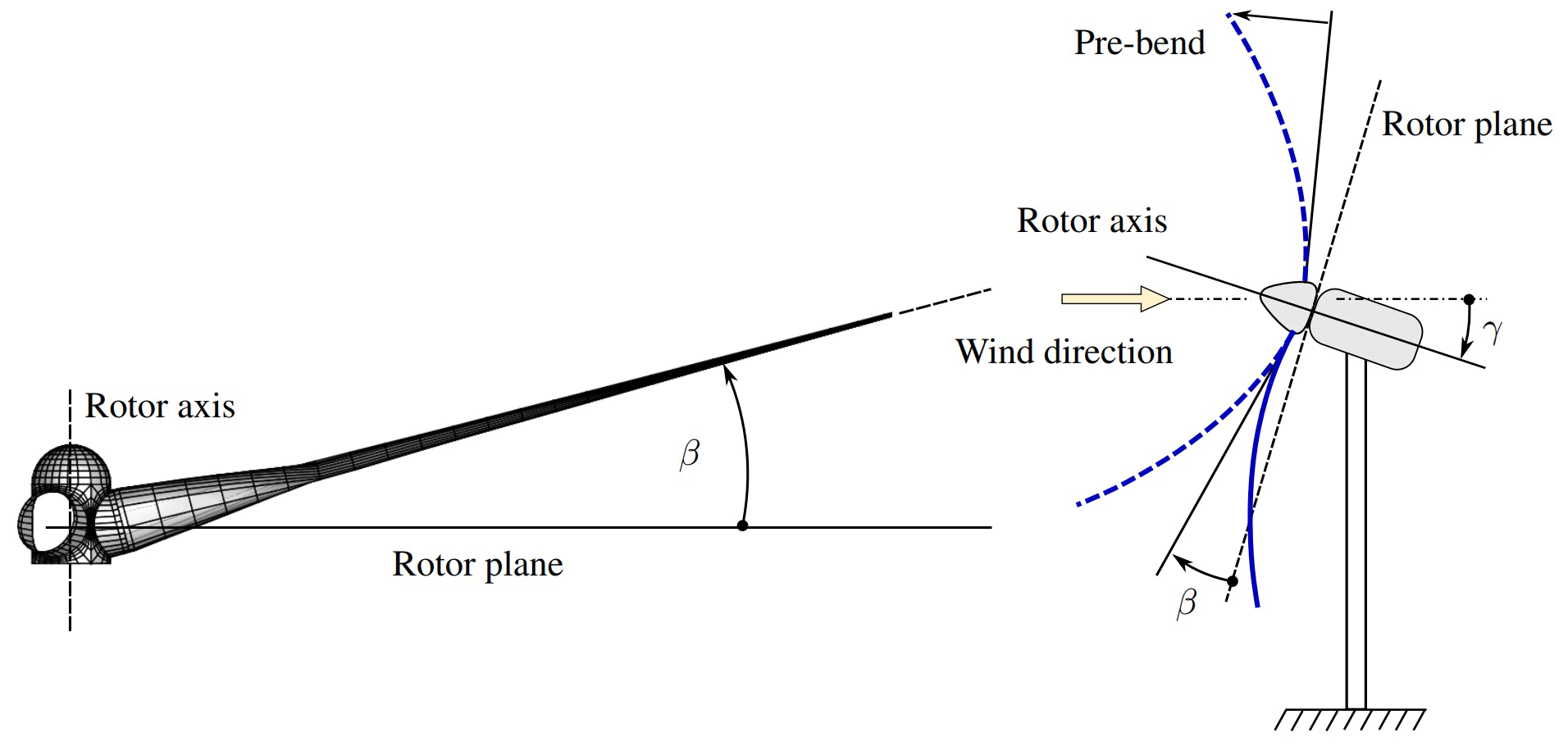
The pitch angle is defined as an inward rotation of the blade leading edge towards the center of rotation of the turbine; in other words, θp is the angle between the tip chord and the rotor plane (see Fig. 17). Moreover, the local pitch is usually expressed as a combination of the pitch angle and the twist angle, i.e., . It should be stressed that Vtotal is the actual wind velocity hitting a blade section located at a distance z from the blade root.
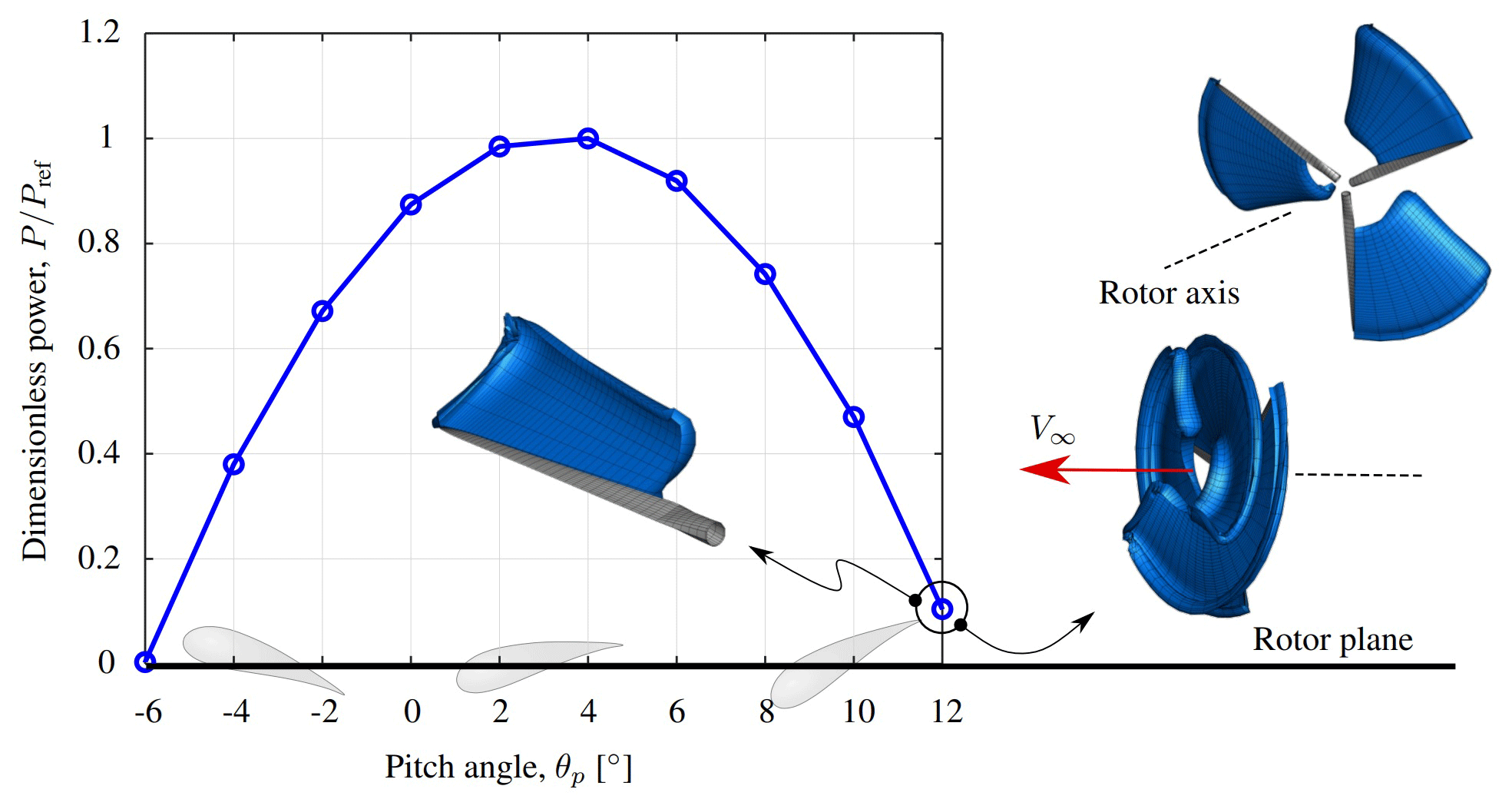
To analyze the influence of the pitch angle on the output power produced for a wind turbine, we carried out a series of simulations considering the same rotor configuration as before and a pitch angle ranging from −6 to 12∘. Figure 18 shows how the output power change as a function of the pitch angle. Note that the power is normalized with respect to the maximum power, .
As it can be observed, the power curve is shifted to the right reaching its maximum at . For this case, a positive pitch angle is needed to get the maximum possible power. As expected, the pitch angle has a significant influence on output power, giving a glimpse of the great controllability associated with this parameter.
4.4 Pre-bend and cone angle study
Besides the twist and distribution of airfoils along the blade, cone angle and blade pre-bend are other two important parameters defining the geometry of a wind turbine rotor. The cone angle β is defined as the angle between the rotor plane and the blade longitudinal axis (see Fig. 19). Its main function is to tilt the rotor so that the blades are no longer at right angles to the nacelle, thus preventing them from hitting the tower as the rotor turns in strong winds (Hau and von Renouard, 2006).
Pre-bending was also primarily conceived to achieve tower clearance, i.e., to make sure that there is sufficient distance between the blade tips and the tower during the wind turbine operation (see Fig. 19). Both methods, coned rotors and pre-bending, require adjustments to the nacelle design.
Here we study how the cone angle and blade pre-bend affect power output independently of each other. To this end, we consider the following two different scenarios: (i) no blade pre-bend and a cone angle ranging from −12 to 12∘ and (ii) a blade pre-bend characterized by a blade tip deflection ranging from −20 % to 20 % and a cone angle . For all cases, the pitch angle is set to zero, . Here, pre-bending is included by using Zuteck's procedure, already described in Sect. 2.2.4, and available in UVLMeshGen. The parameters of the Zuteck formula are listed in Table 7.
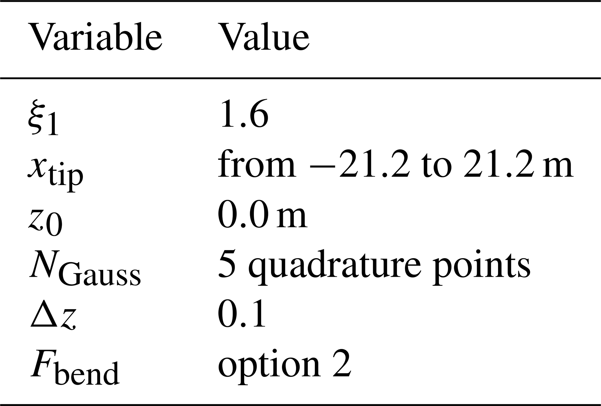
The reader can find an explanation of such parameters in Appendix A, Table A5. Both tip deflection x1 and cone angle range were calculated with the goal of having a tip blade deflection of 20 % of the rotor radius (i.e., blade length + hub radius = 106 m). For this study we selected again the SNL100-00 wind turbine operating under the same working conditions and spatial–temporal discretizations as in the previous subsections. For this study, the power is normalized with respect to the power obtained for the reference configuration, which is characterized by no pre-bending and cone angle .
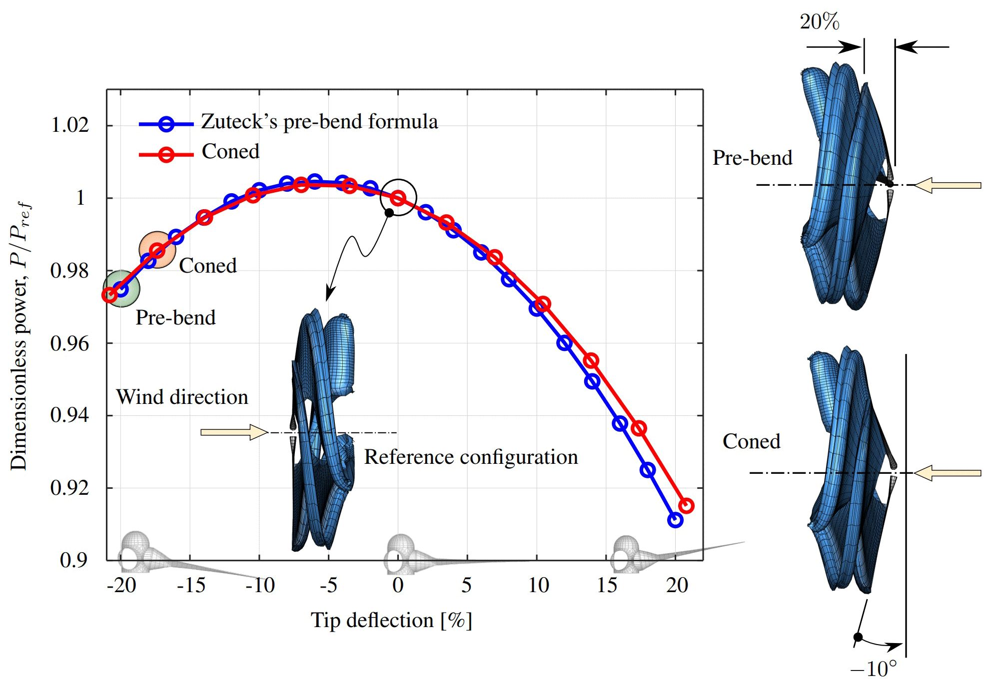
Figure 20 shows that blade pre-bending or cone angles affect the power output in a similar way. As it can be observed, the power curves are both shifted to the left reaching their maximum at and m. These findings suggest that those rotors having downwardly inclined blades provide higher performance than those with positive cone angles or positive blade pre-bending. However, such sorts of rotors are of no practical importance since in general cone angles and pre-bending are measures in order to achieve tower clearance. Although the results obtained in this study are original, they are only valid for the wind turbine considered here since there is not enough information available to draw general conclusions.
4.5 Aerodynamics of full wind turbines
In this subsection, we present some aerodynamic simulations of two well-known wind turbine concepts. One of them is the DTU 10 MW reference wind turbine developed by DTU Vindenergi (Institut for Vindenergi) (Bak et al., 2013). The second turbine considered here is the SNL100-00 13.2 MW wind turbine concept developed by Sandia National Laboratories (Griffith and Ashwill, 2011).
According to the technical report Bak et al. (2013), the DTU 10 MW wind turbine was designed for offshore siting for an IEC class 1A wind climate, which is characterized by a rated wind speed of 11.4 m s−1, minimum rotor speed of Ωmin=6.0 RPM, and maximum rotor speed of Ωmax=9.6 RPM. In addition, the DTU 10 MW blades have pre-bends in order to guarantee tower clearance. In Table 8 we list the main geometric and kinematic parameters used to compute the power and wake evolution of the DTU 10 MW wind turbine. A complete geometric description of the wind turbine is available in Bak et al. (2013). Moreover, the reader can obtain the configuration files for generating the aerodynamic grid and kinematics for this study case in our UVLMeshGen GitHub repository (Roccia, 2023).
Table 8DTU 10 MW wind turbine – geometric and kinematic parameters.
In Fig. 21 we present an aerodynamic simulation of the DTU 10 MW wind turbine obtained by using the VLMSim flow solver. The working parameters correspond to those specified in Table 8. Peaks appearing in the power curve arise as consequence of the blades passing through the tower influence region. According to the simulation parameters, the period of each revolution is 6.316 s, thus giving three peaks per revolution. Such a result is in total agreement with the fact of having the passage of three blades through the tower influence region per revolution.
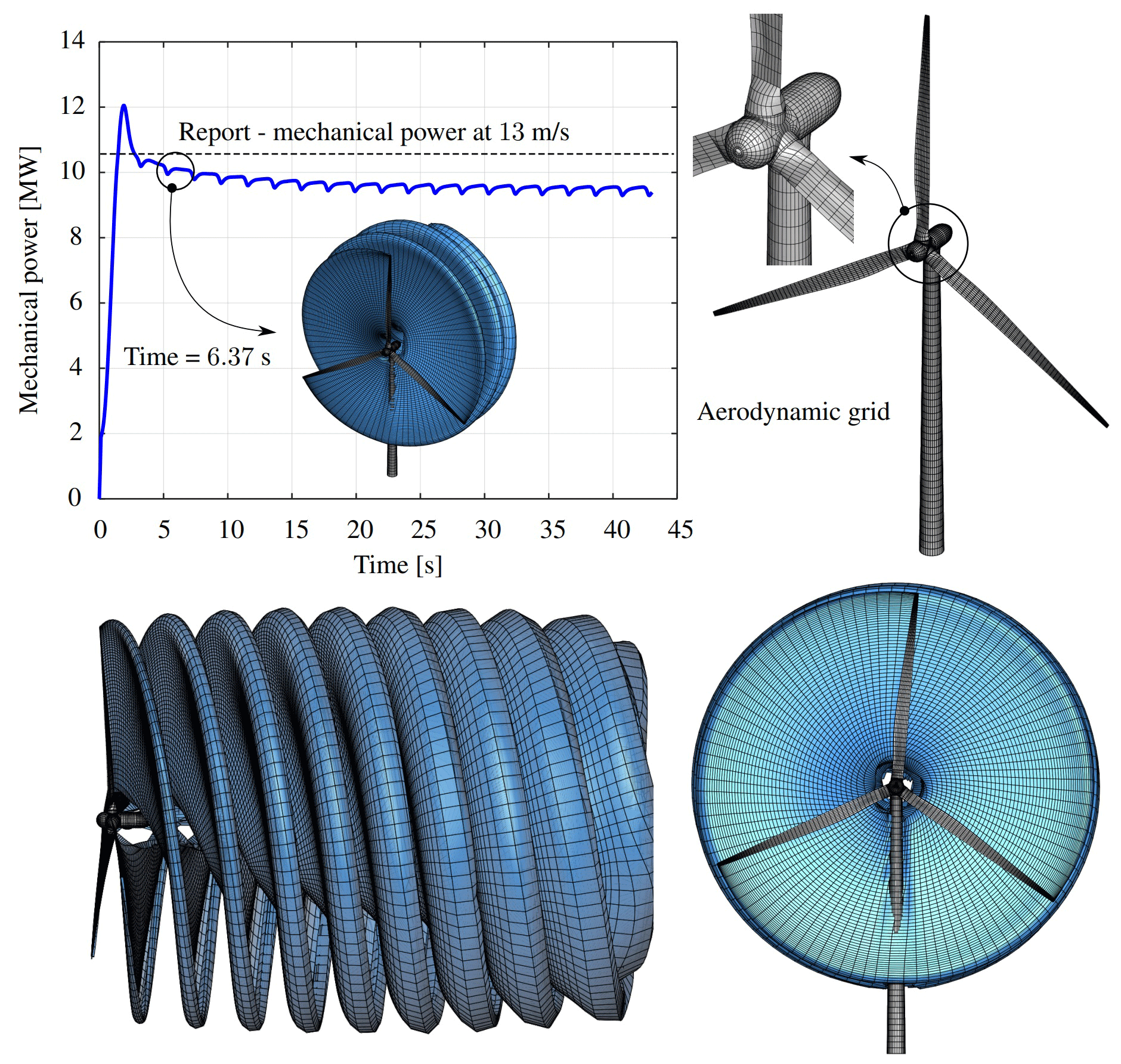
Such a phenomenon is recognized as an aerodynamically unsteady region, where the flow angle and velocities are significantly affected. As the upwind turbine blades pass through this region of velocity perturbations, the flow seen by the blade is directly modified, thus resulting in periodical drops of the lift forces and, therefore, a power curve with peaks. This finding is justified from a physical point of view, and its magnitude could be influenced by effects of numerical origin, for which more studies are required to understand this phenomenon.
Another aspect worth mentioning is the interaction of the wakes with the tower. As can be seen in Fig. 21, it may seem that the flow solver considers some sort of wake rupture as used by Gebhardt et al. (2010). However, VLMSim does not have such a capacity, but it can handle wake–body interference to some extent by using a vortex core-growth strategy based on the Lamb–Oseen model (Bhagwat and Leishman, 2002; Roccia et al., 2018). This add-on allows for diffusing vortex segment intensities to handle situations in which two or more vortex segments are getting extremely close. Despite the fact that both methods are radically different, they predict very similar behaviors in terms of the peaks observed in the aerodynamic loads (consequence of the tower shadow). Furthermore, it should be emphasized that the in-house solver VLMSim has been extensively verified and validated in Verstraete et al. (2023).
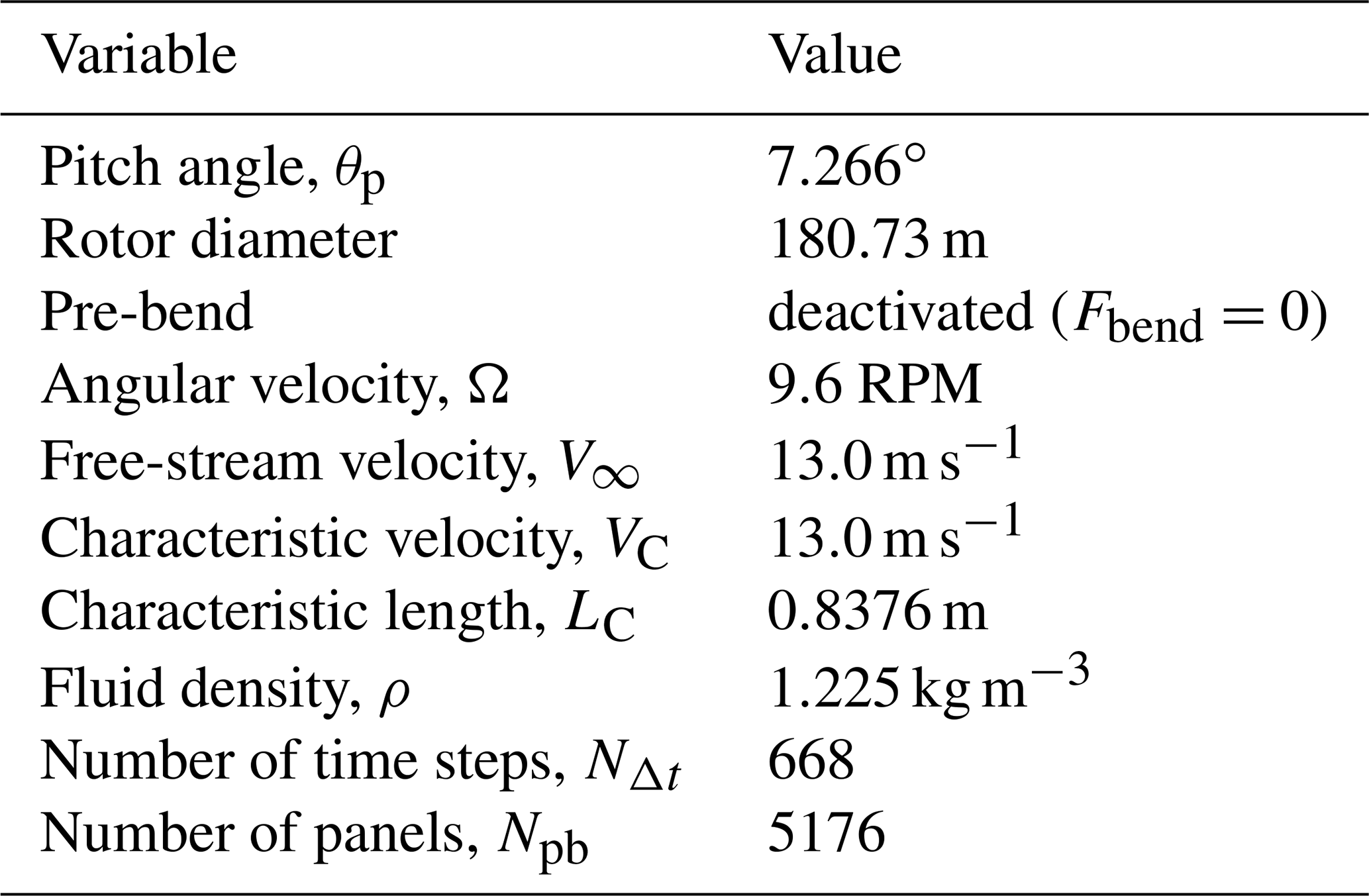
The second wind turbine adopted here is the Sandia 13.2 MW SNL100-00 with a 100 m blade length, which is based on the NREL 5 MW model (Jonkman et al., 2009). The cut-in, cut-out, and rated wind speeds are 3.0, 25, and 11.3 m s−1, respectively. The maximum rotation rate of this variable speed machine is Ωmax=7.44 RPM. In Table 9 we list the main geometric and kinematic parameters used to compute the power and wake evolution of this wind turbine. Moreover, the reader can obtain the configuration files for generating the aerodynamic grid and kinematics for this study case in our UVLMeshGen GitHub repository (Roccia, 2023).
Table 9Sandia 13.2 MW SNL100-00 – geometric and kinematic parameters.
In Fig. 22 we present the time series of the output power for the SNL100-00 wind turbine together with the spatial evolution of the wake. The power after 40 s of simulation is around 12.4 MW (steady state), this value being 6 % less than the theoretical power predicted in the technical report. This difference may be attributed to different sources. First of all, we are considering a constant pitch angle throughout the simulation, when in fact this machine operates with a variable pitch angle. Second, the report utilizes a version of the low-fidelity and well-known blade element momentum theory to predict the aerodynamic forces, which can lead to some differences when compared to more accurate methods such as mid-fidelity vortex-based approaches. However, the results included here are not aimed at an exhaustive aerodynamic study of the aerodynamic performance of turbines but to show the capacity of the UVLMeshGen to generate suitable UVLM meshes in a fast and versatile way.
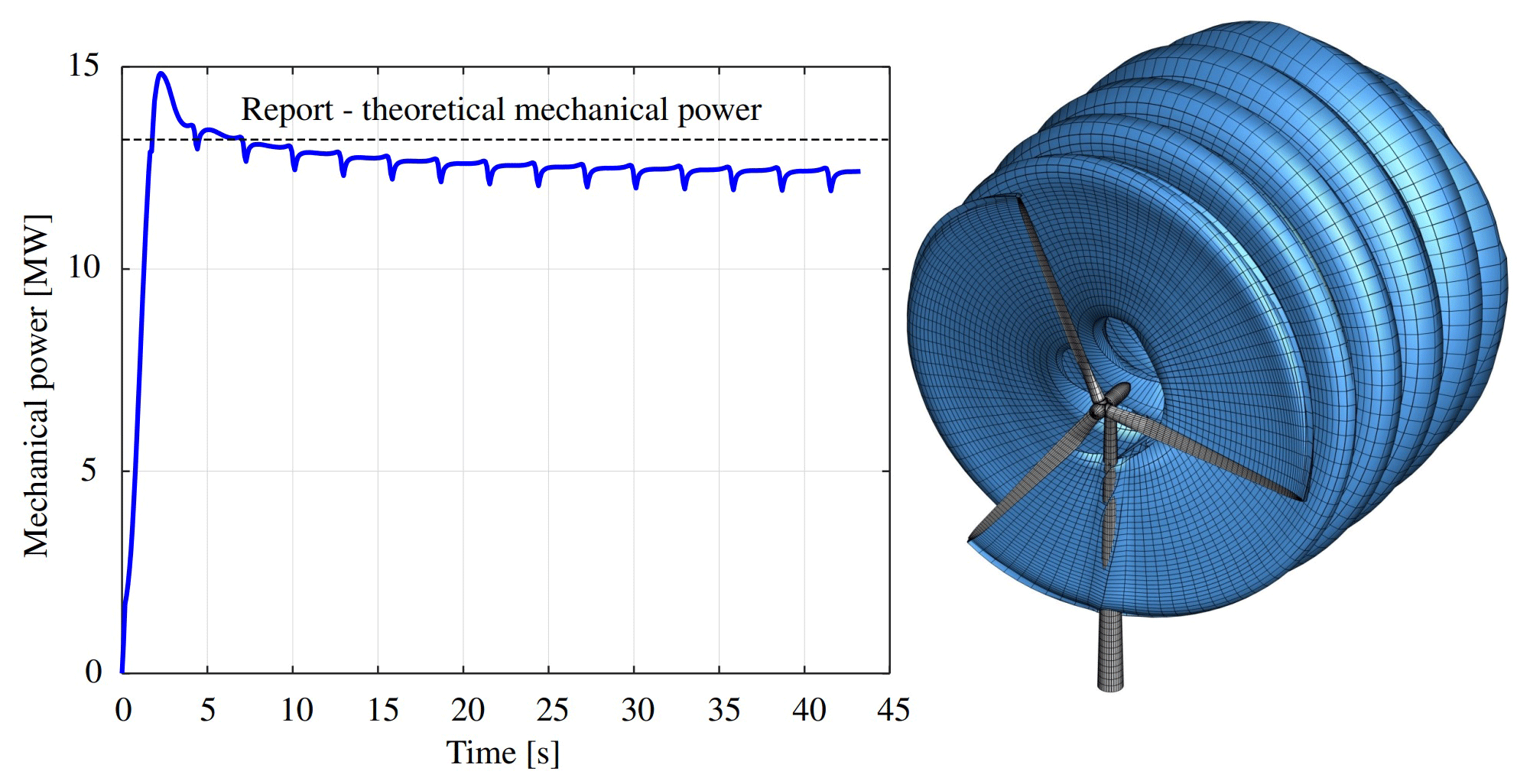
Finally, the peaks observed in the power curve have the same origin as those discussed above for the DTU 10 MW wind turbine; however their magnitudes are slightly larger. As previously stated, although the appearance of these peaks has a well-founded physical explanation, their magnitude may not be entirely correct and may be affected by numerical issues.
4.6 Wind energy farms
This subsection has a main goal to show the versatility and capacity of the meshing tool developed through the generation of two hypothetical wind farms. These examples give a glimpse the scalability power of the UVLMeshGen in generating aerodynamic grids of heterogeneous parks consisting of an arbitrary number of wind turbines, including the terrain modeling (for both onshore and offshore farms). The meshes obtained from UVLMeshGen are used as input for the VLMSim solver to carry out qualitative aerodynamic simulations of such wind farms.
4.6.1 Onshore wind farm
Here we focus on modeling an onshore wind farm consisting of four wind turbines, of which two turbines are of the DTU 10 MW type and the other two are of the SNL100-00 type. Figure 23 shows the layout of the wind park, and Table 10 lists the main geometric and kinematic parameters used to carry out an aerodynamic simulation of the entire wind farm.
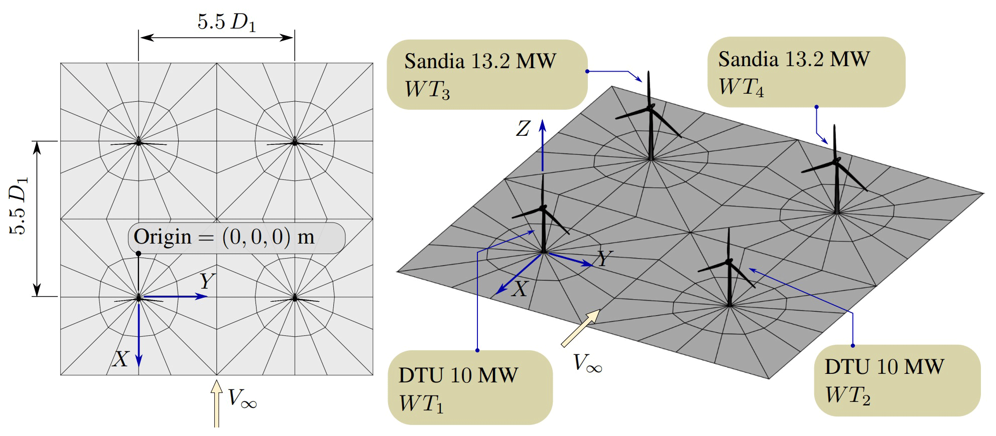
Table 10Onshore wind farm – geometric and kinematic parameters
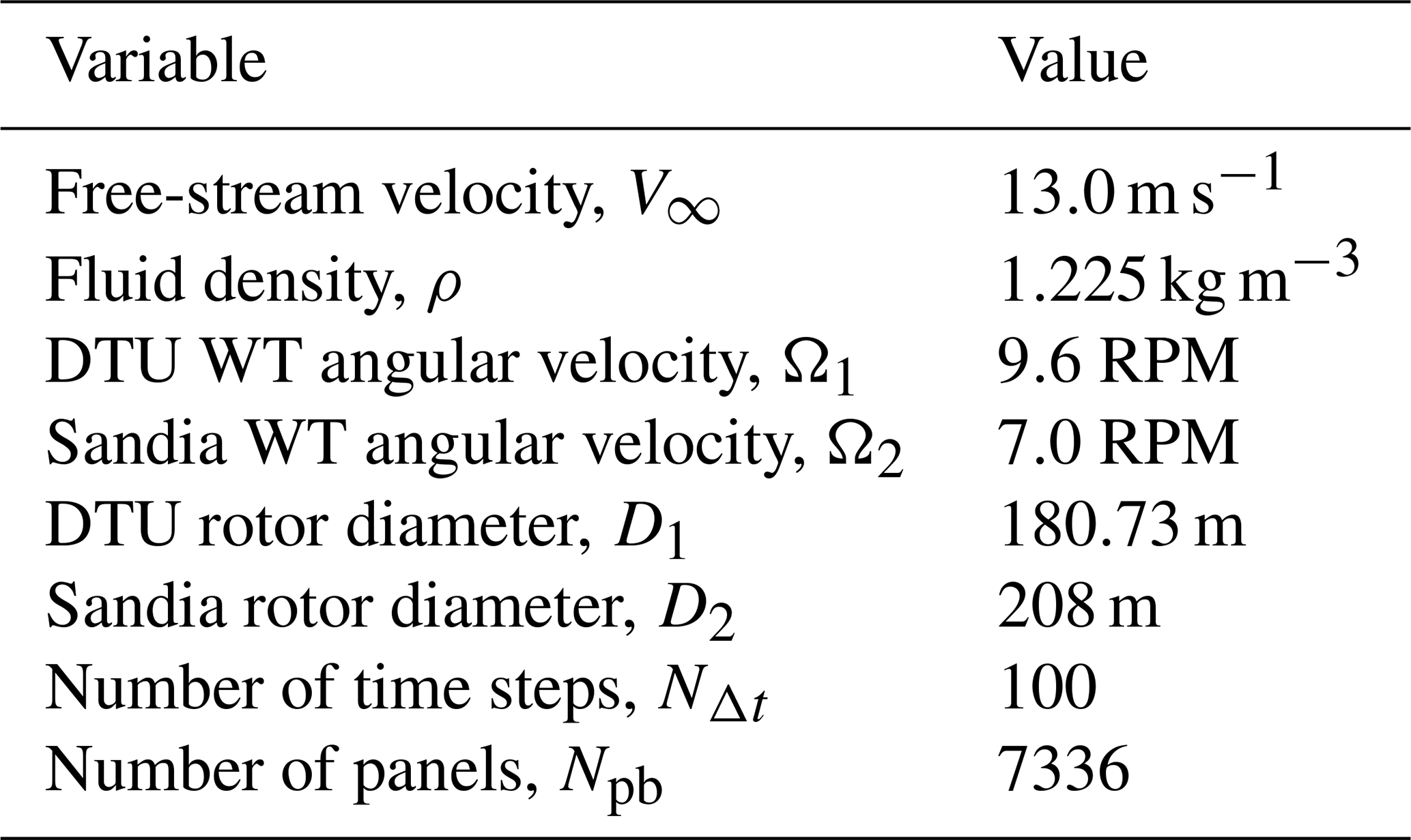
As can be seen from the schematic, the grid used is relatively coarse in order to reduce the computational cost associated with the aerodynamic simulation. In UVLM-based solvers there are mainly two time-consuming processes: (i) the computation of the circulations, which requires solving a linear system of dimension Npb×Npb, and (ii) the convection of the wakes. Although for systems discretized into a large number of panels the solution of the linear system may take longer initially, as time evolves, the wake convection undoubtedly becomes the bottleneck of the aerodynamic simulation.
Figure 24 shows the aerodynamic simulation for the entire onshore wind farm after 100 time steps. Clearly, the wakes emanating from the DTU wind turbine develop more than those shed from the Sandia machine because of the different angular velocities. However, the time step used for the whole farm is the same and its value is determined according to what is explained in Sect. 3.5. As an example and to bring up the computational cost of simulating wind turbine farms, the simulation time for 100 time steps of the farm described above took 28 h on the desktop computer described at the beginning of this section.
4.6.2 Offshore wind farm
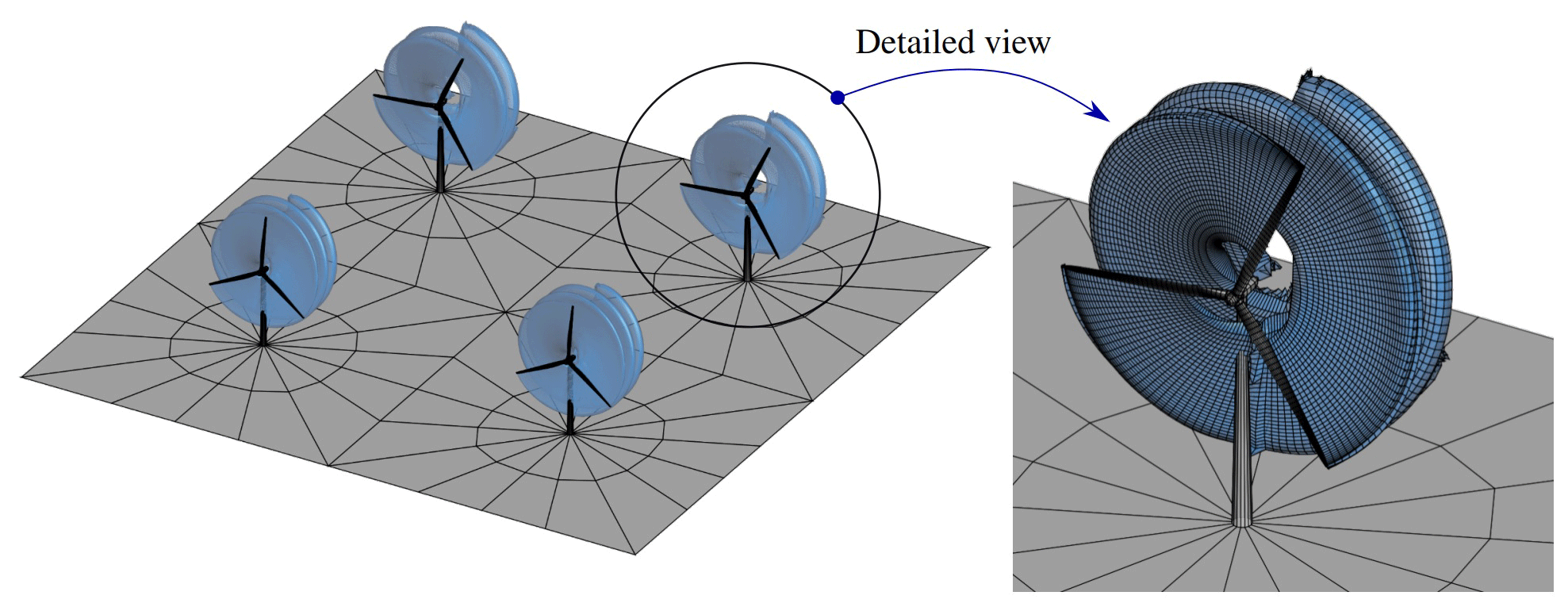
Finally, we present the modeling of an offshore wind farm consisting of nine IEA 15 MW wind turbines. This reference wind turbine is a Class IB direct-drive machine, with a rotor of 240 m and a fixed-bottom monopile support structure which was jointly developed between the National Renewable Energy Laboratory and the Technical University of Denmark (Gaertner et al., 2020). The terrain was modeled with a sinusoidal function to simulate an ocean wave profile, similar to the example shown in Fig. 13, to incorporate sea level as a boundary for the flow solver. Although this wave does not have movement (or kinematics), it is not the objective of this work to carry out an exhaustive study of offshore farms but rather to show the versatility of the meshing tool. Figure 25 shows the layout of the offshore wind park, and Table 11 lists the main geometric and kinematic parameters used to carry out an aerodynamic simulation of the entire wind farm.
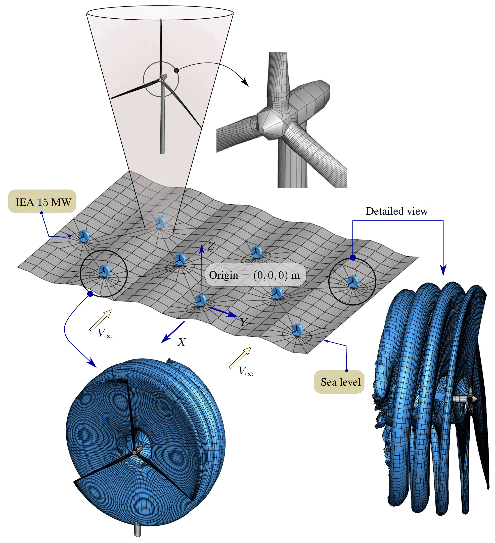
Table 11Offshore wind farm – geometric and kinematic parameters
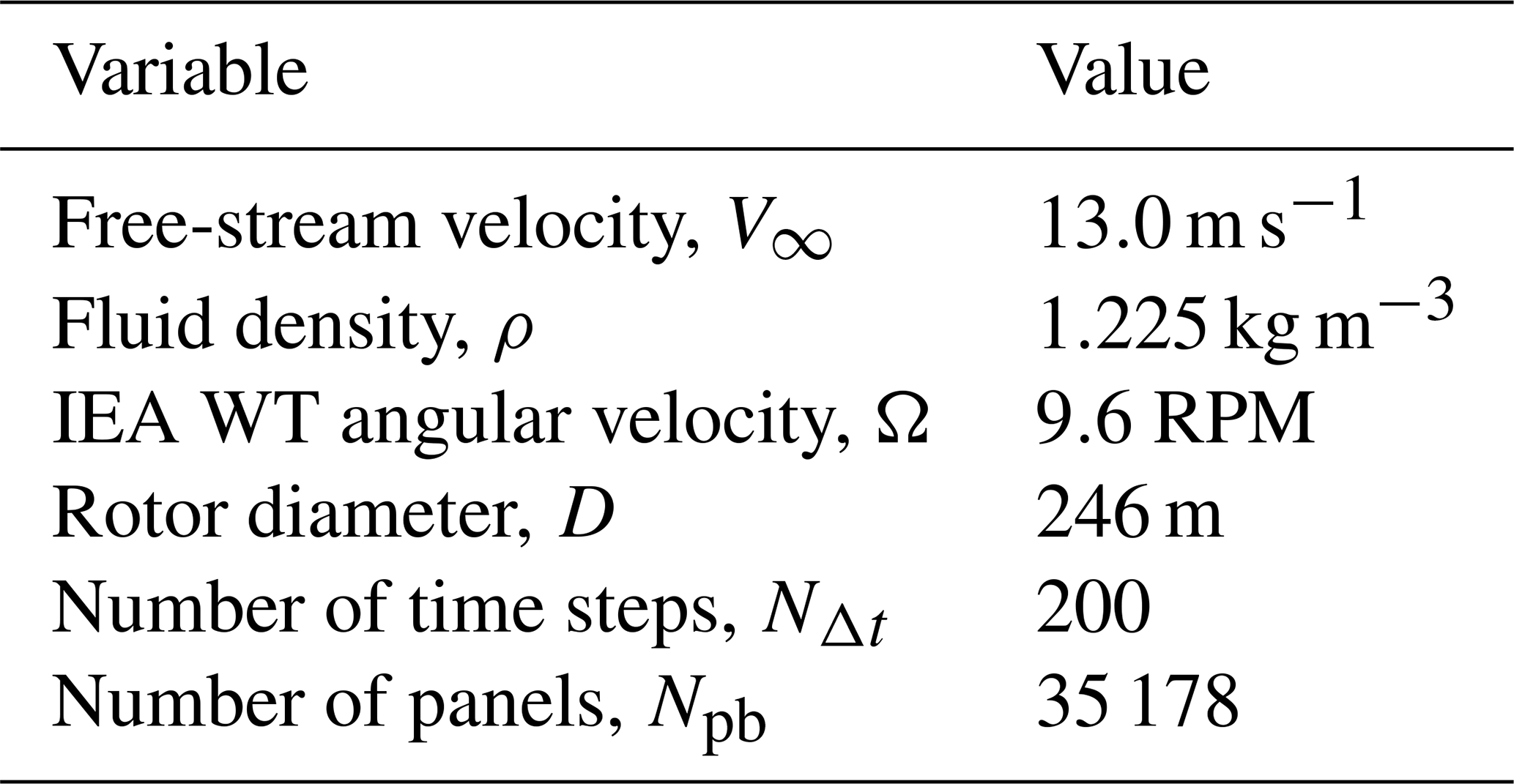
Figure 25 shows the aerodynamic simulation for the entire offshore wind farm after 200 time steps. As before, the grid used for this farm is coarse in order to reduce the computational cost associated with the aerodynamic simulation. Even with a coarse mesh, the total number of panels is around 35 000, which translates into an aerodynamic matrix of the order of 1×10⁹ elements. The solution of the linear system plus wake convection has increased the computational cost for this example from 28 h (onshore farm) to 96 h.
Although the aerodynamic simulations of wind turbine farms presented above are purely qualitative in nature, they do highlight the time-consuming problem associated with these types of studies. Although these cases have been run on a relatively outdated desktop computer, it is necessary to implement methods to speed up UVLM-based solvers. On this basis, it is essential to explore the use of the fast multipole technique in order to reduce from O(n2) to O(n) and O(nlog n) the number of operations performed evaluating the Biot–Savart law (Willis et al., 2007; Bogateanu et al., 2010; Deng et al., 2021), or the implementation of parallelization and vectorization algorithms in graphics processing units (GPU) using CUDA for example (Chabalko et al., 2013; Türkal et al., 2014).
In this article, we presented a detailed description of the geometric modeling and computational implementation of an interactive and versatile UVLM-oriented mesh generator for wind turbines and onshore–offshore wind farms. The meshing tool was developed entirely in MATLAB® and easily adaptable to GNU OCTAVE. We also provided a full explanation of the input data needed by the tool, including tables where the reader can find a description of all the variables and their names in MATLAB®. The output data provided by UVLMeshGen, nodal coordinates and connectivity arrays, were successfully used by the UVLM-based solver VLMSim. In addition, the meshing tool was robust when generating different configurations of WTs and WFs according to airfoil data, geometric parameters, terrain topography, wind farm layouts, and meshing requirements. UVLMeshGen has been tested with a large number of examples and has proven to be efficient in building aerodynamic grids of onshore–offshore wind turbines and wind farms. Furthermore, UVLMeshGen was intensively used to generate all the meshes for the aerodynamic simulations included in Sect. 4. Although such results were mainly conceived to show the capabilities of the developed meshing tool, the versatility of the mesh generator allowed us to investigate different rotor configurations, whose aerodynamic characteristics are not commonly found in the literature. Among these findings, coning angle and pre-bending were found to affect the output power in a similar way.
Although a freely available meshing tool such as UVLMeshGen may significantly contribute to the community focused on wind farm aerodynamic simulations, it still has important limitations that should be addressed in the future as a follow-up to this contribution. Among the most important improvements that can be made we identify (i) the meshing of different types of substructures (for offshore wind energy), (ii) the meshing of the blade considering its thickness, (iii) the kinematics of the substructure, and (iv) the kinematics of the sea surface (to simulate waves). Finally, we encourage the community to actively participate in this open project related to providing and improving meshing tools intended for potential flow solvers for the wind energy sector.
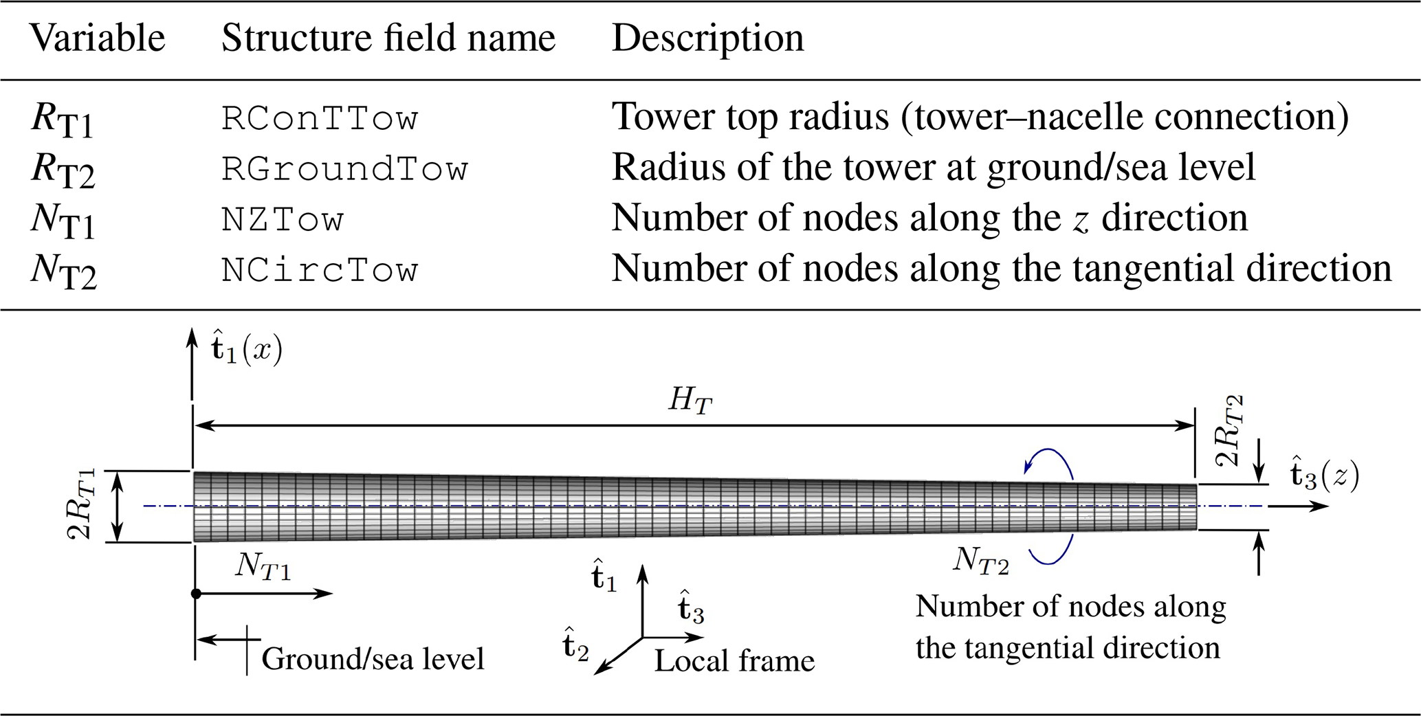
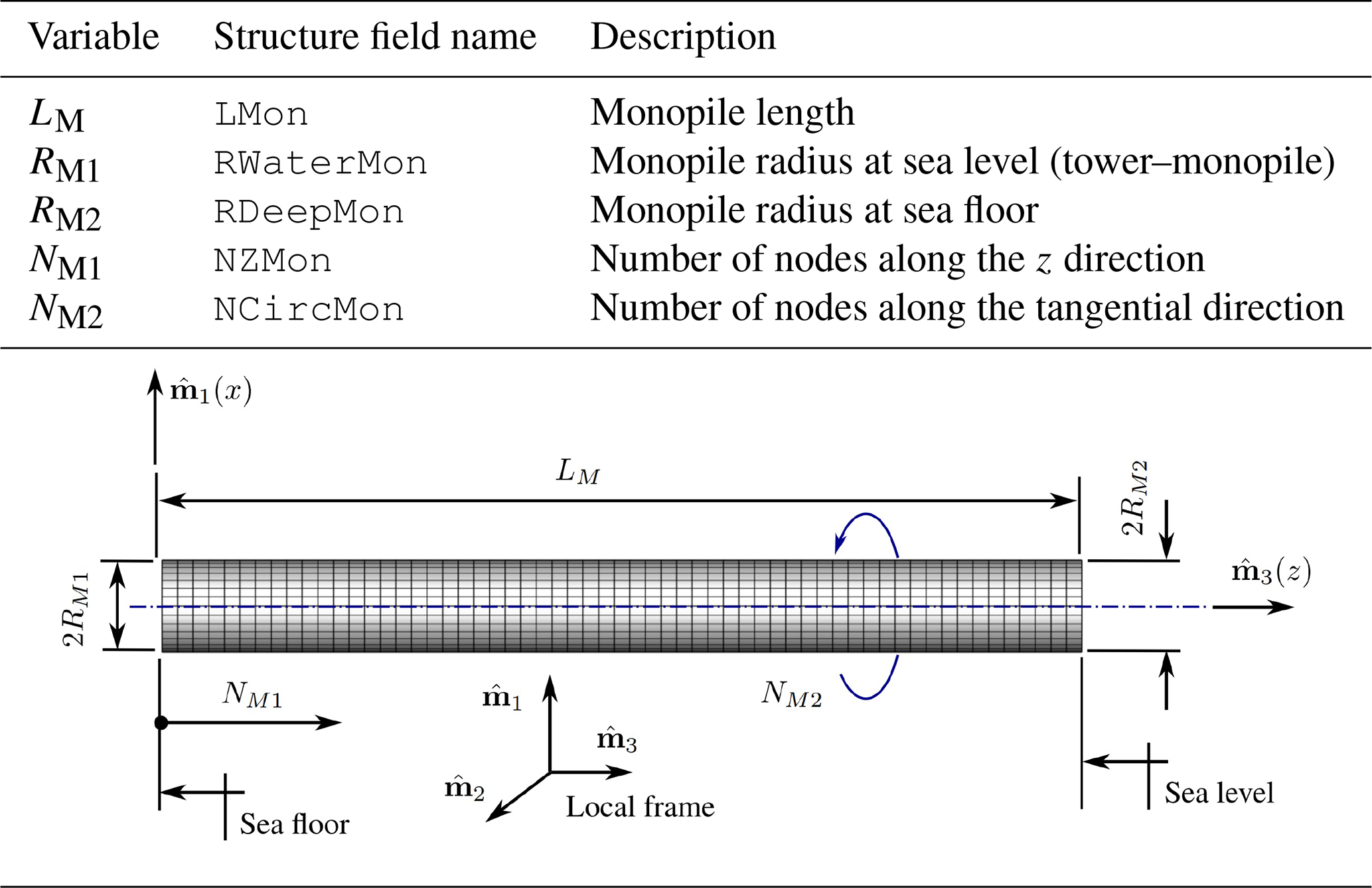
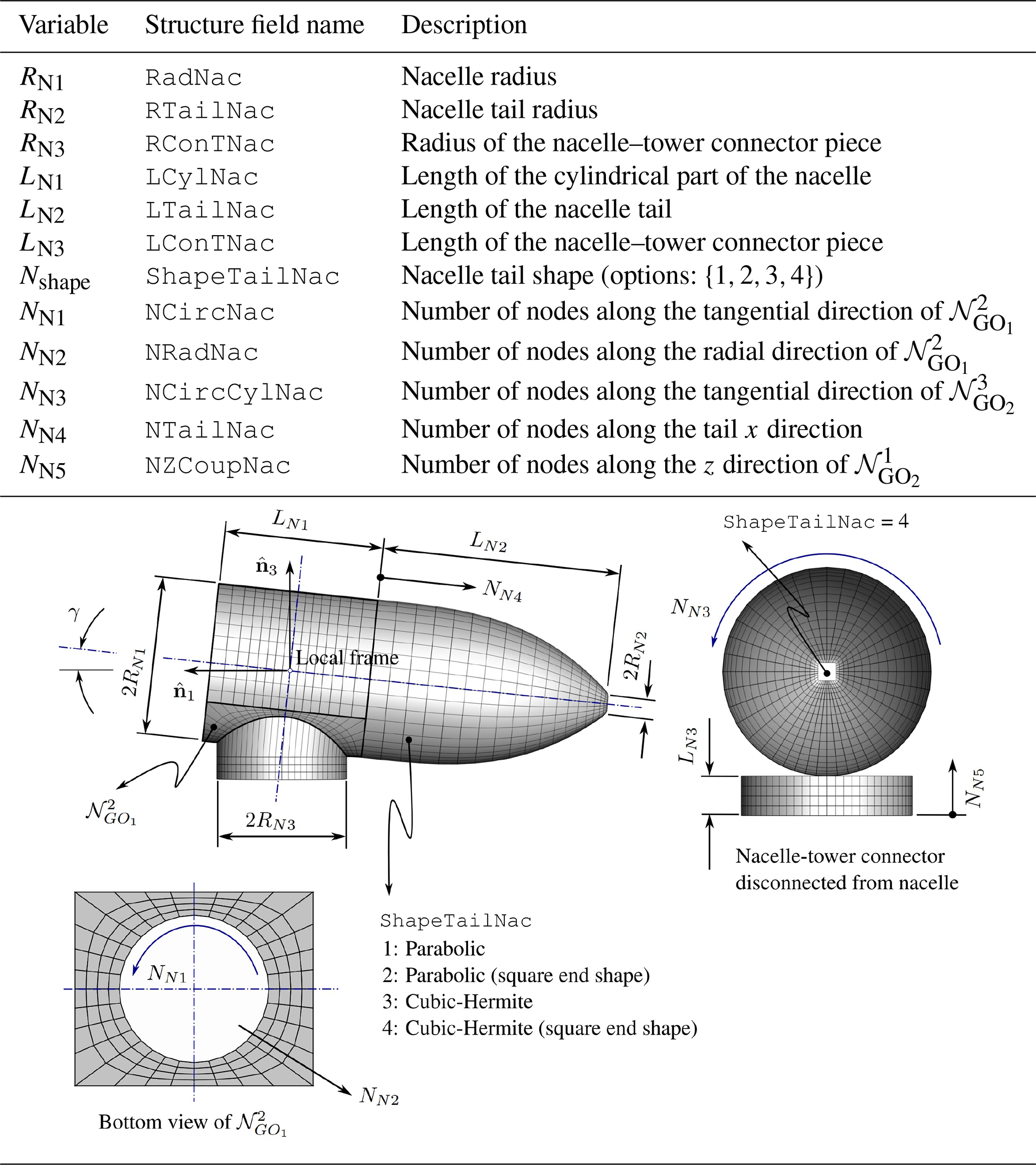
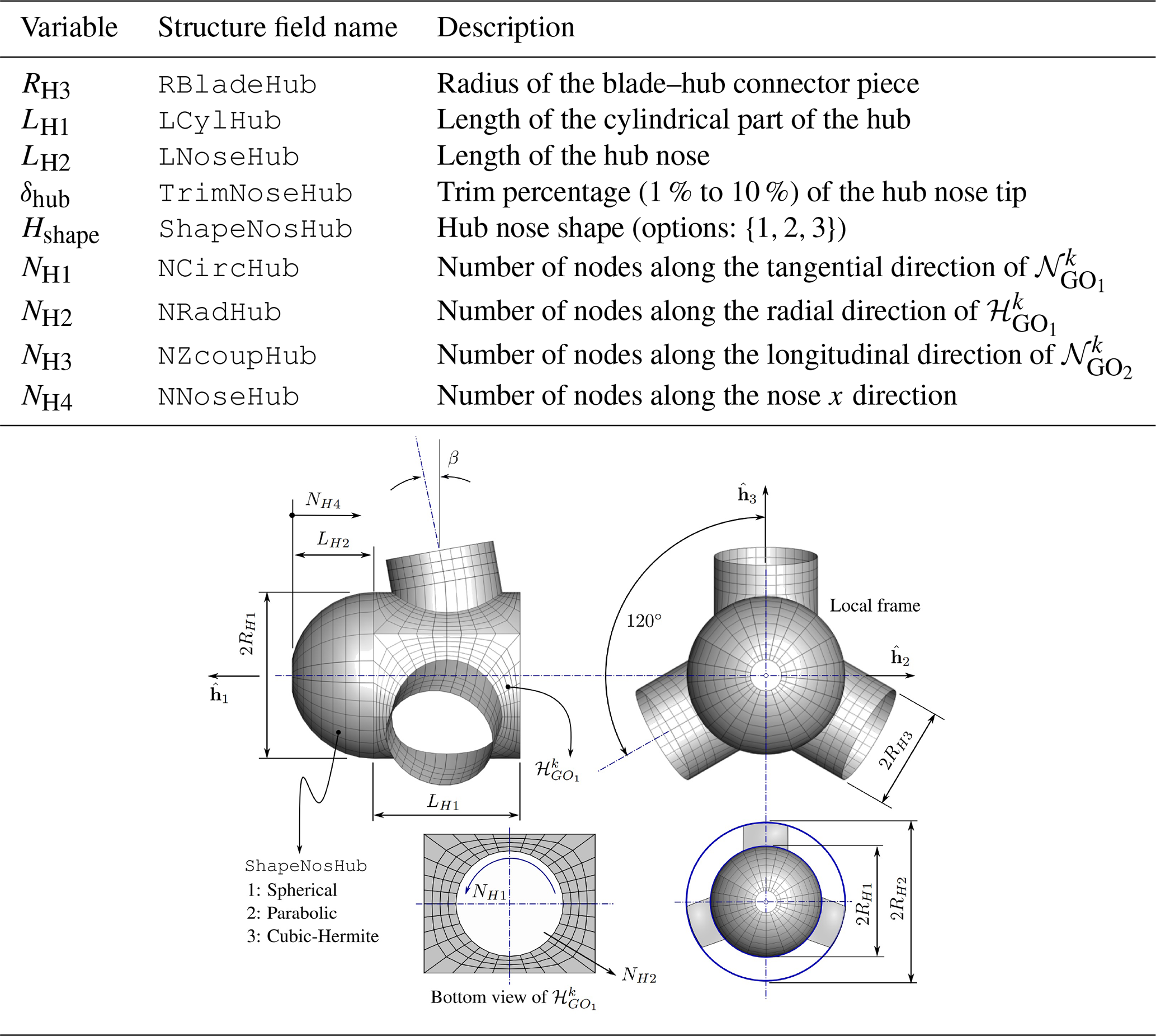
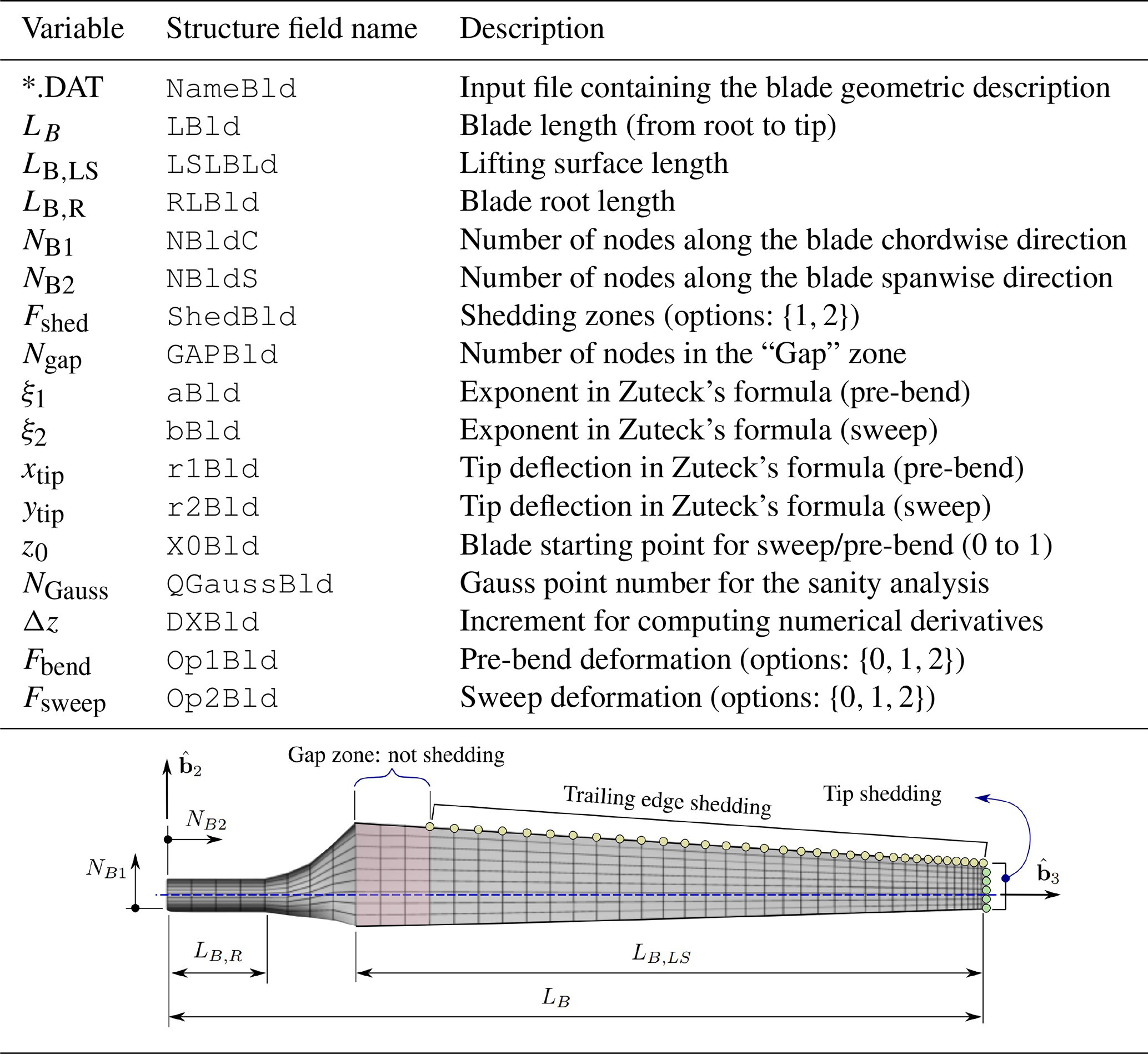
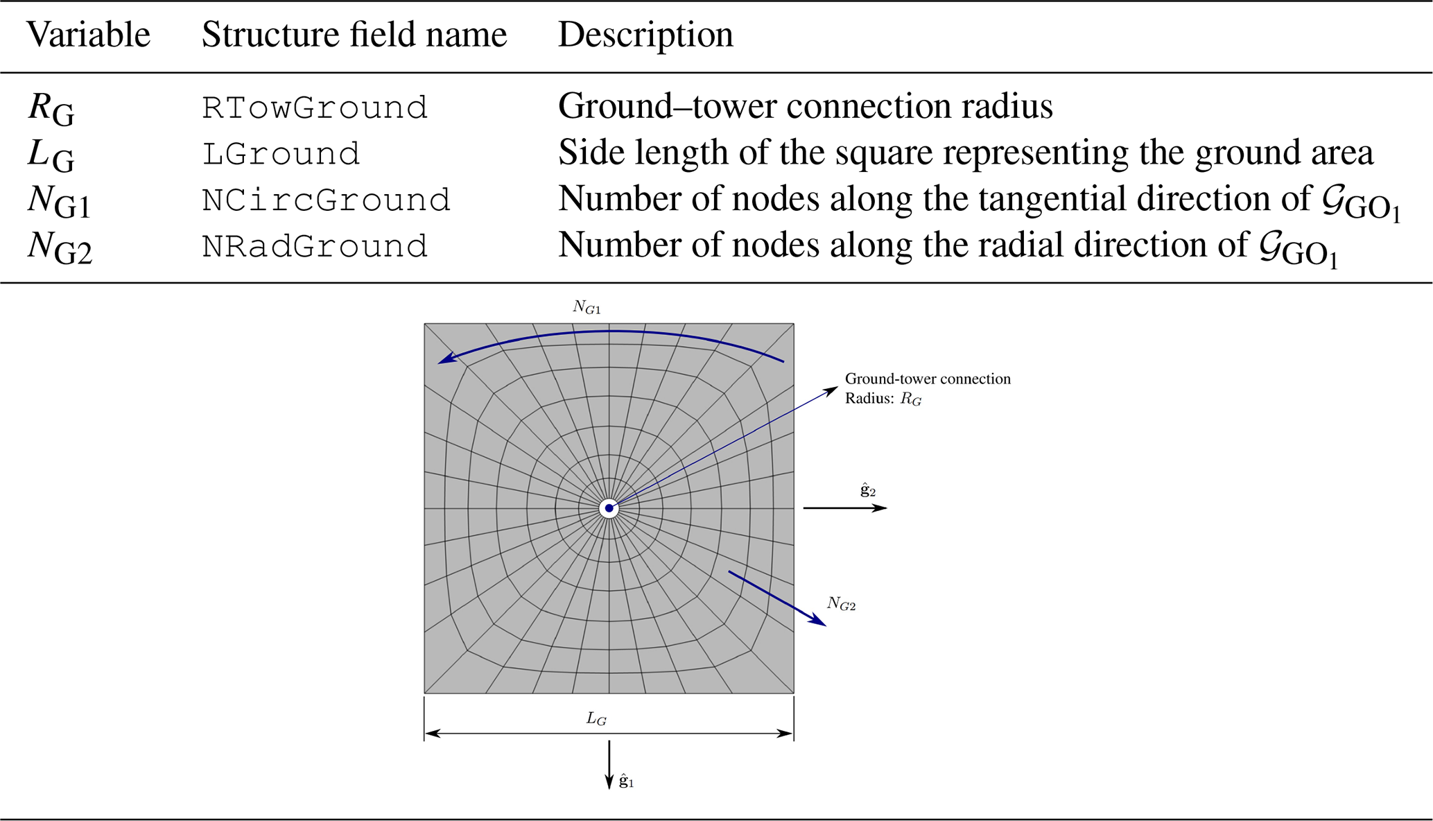
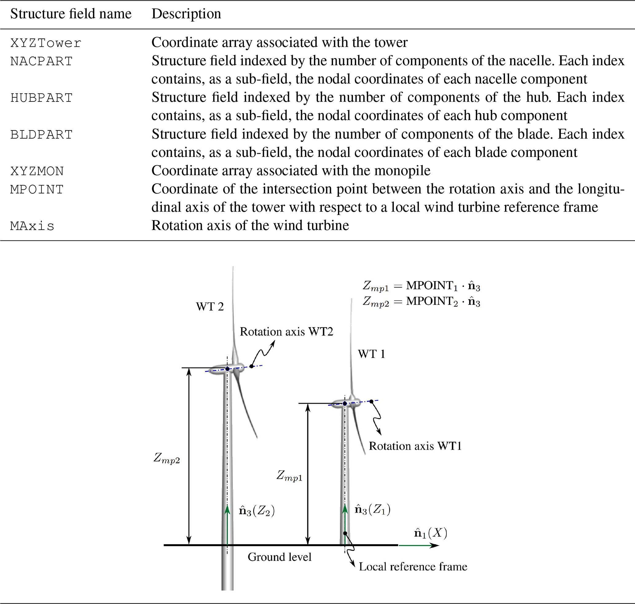
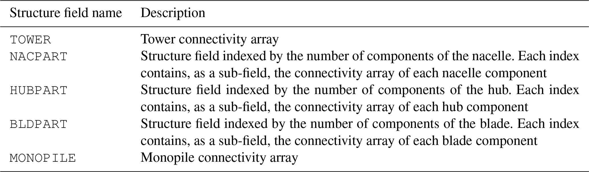
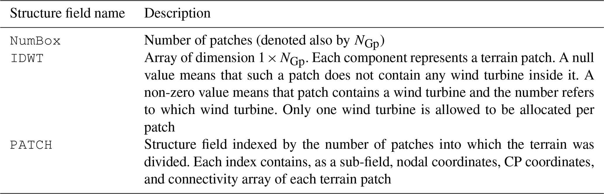
Table B4KINEMATICS(i).WT – main fields and substructure variables.
In this appendix, we present a brief review of the unsteady vortex-lattice method in order to highlight the relationship between the geometric modeling introduced in previous sections and the data needed by UVLM-based solvers when it comes to aerodynamic simulations of complex aeronautical/mechanical engineering applications – here wind energy farms in particular.
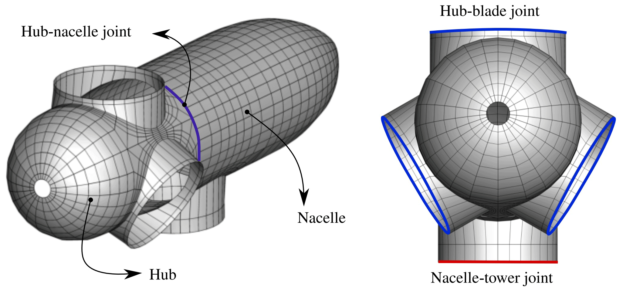
According to Preidikman (1998) and Katz and Plotkin (2001), in UVLM-based computational implementations, the continuous bound-vortex sheets are discretized into a lattice of short, straight vortex segments of circulation Γ(t). Such segments divide ∂ℬ into a finite number of elements Bk (also called panels or boundary elements). The wakes shed from the separation zones (trailing edges (TEs), wing tips or blade tips, and leading edges (LEs)) are also represented by vortex lines. In Fig. C1 we present a schematic representation of the vortex lattices for the hub–nacelle assembly of a wind turbine.
Following Verstraete et al. (2023), the complete boundary of an aeronautical–mechanical system is geometrically decomposed into a finite set of boundary elements , such that
where , NB is the number of bodies, , and is the number of panels associated with each aerodynamic subgrid 𝒜i. Then, the total number of panels used to discretize the whole surface 𝒜 is calculated as .
It is well known that UVLM solvers strongly depend on the quality with which lifting and non-lifting surfaces are represented. Wind turbines, and even more so wind farms, are characterized by very complex geometries in general (rotor, blades, terrain topography, etc.), and therefore robust and precise meshing processes are needed to ensure a correct estimation of aerodynamic loads. In this sense, it has been found that the geometric entities GO1 and GO2, described in Sect. 2, allow us to generate all the grids and subgrids associated with sets 𝒜i.
As mentioned above, the edges of each are represented by straight, finite vortex segments of circulation Γ(t), whose contribution to the velocity field is computed through a discrete version of the Biot–Savart law:
where r1 and r2 are the position vectors of the point where the velocity is being evaluated relative to the ends of the straight vortex segment, , and δc is a cut-off parameter, which is introduced to remove its singular kernel. Although introducing the term into Eq. (C2) is interpreted as essentially an ad hoc technique (Chorin, 1994; van Garrel, 2003), it has been proven to work satisfactorily well in practice.
C1 Aerodynamic influence coefficients
In UVLM-based codes, the non-penetration condition is generally imposed either at the geometric centers of each (the so-called control or collocation points, CPs) or at of the panel chord (Katz and Plotkin, 2001), resulting in a linear system of algebraic equations (usually with time-varying coefficients). The unknowns are the circulations around the individual bound vortex segments; however, the linear system can be rewritten in terms of vortex ring circulations Gj(t), thus reducing the size of the problem (Verstraete et al., 2023). Under these assumptions, the linear system takes the following form:
where aij(t) are the aerodynamic influence coefficients, is the unit vector normal at the ith control point, VW is the velocity induced by the free-vortex lattice, VS is the velocity of the solid, V∞ is the free-stream velocity, A(t) is the aerodynamic influence matrix, G(t), and RHS(t) is the right-hand side, which collects the contributions of the wake, free-stream, and body velocities along the normal direction at each CP.
As it can be observed in Eq. (C3), solving for the unknown circulations requires knowing the body velocities VS at each control point. Such velocities depend on the kinematics imposed on the rotor (including yaw and pitch motions, if any), substructure kinematics, and sea level surface motions for offshore wind turbines. Consequently, the position and velocity data provided by the kinematic module of the UVLMeshGen (described in Sect. 3.5) play a fundamental role in developing high-quality aerodynamic simulations of arbitrary onshore–offshore wind farms.
C2 Wake convection
In order to formalize the convection process, let us consider 𝒱i for be a set of panels representing the wake shed from shedding zones (SZs) of 𝒜j∈𝒜, such that
where , NW⩽NB is the number of lifting surfaces, , and is the number of vortex rings in 𝒱i. Then, the total number of free-vortex rings at time t is determined as .
Once the circulations Gj(t) are calculated, the wakes are convected to their new positions and new vortex segments are propagated into the free-vortex lattices. Because all the quantities involved in the convection are functions of time, the question of which instantaneous quantities to use in the approximation is raised. There are several options; for example, one can use the quantities that were calculated at the previous time step, the present time step, or their averaged values for the two time steps. In all cases except the first, iterations are needed, which increase the computational cost. Kandil et al. (1976) showed that explicit one-step methods are stable, and there are little differences in the computed results when compared with higher-order procedures. In this respect, here we use an explicit first-order method to propagate the wake:
where the subscript “node” is introduced to refer to the corners of a vortex segment, Nnw(t) is the number of aerodynamic nodes in 𝒱, and Δt is the time step. The vector Vnode(t) collects the contributions from all surface vortex rings , all free-vortex rings , and the free-stream velocity.
C3 Aerodynamic loads
Among the several procedures proposed in the literature for computing aerodynamic loads by using the UVLM, we can mention the Joukowski approach (Simpson et al., 2013; Lambert and Dimitriadis, 2017), the Katz approach (Katz and Plotkin, 2001; Lambert and Dimitriadis, 2017), and an alternative formulation based on the Katz method developed at Virginia Tech (VT) (Preidikman, 1998). Here we present a quick review of the VT approach for predicting aerodynamic forces.
The VT approach is similar to that proposed by Katz. It computes the pressure jump across the bound-vortex lattice by using the Bernoulli equation for unsteady flows:
where Dp is the pressure jump, ρ is the fluid density, stands for partial time derivative, , , ∇(⋅) is the Nabla operator in ℝ3, φ is a scalar potential, Ψ is a vector potential, and ψ is another scalar potential such as . The component of the velocity field coming from the scalar potential is irrotational, while any vorticity contribution to it is captured by the vector potential component.
After some algebraic manipulations, the pressure jump for the k element in 𝒜 can be expressed as follows:
where is the “mean” velocity, which does not recognize the presence of the local vorticity, and ΔVk represents the jump in the tangential velocity across Bk. Finally, the vector force on Bk, Fk, is obtained as the product of Eq. (C7) times the element area times the normal unit vector at CPk:
For more details about the theory as well as implementation aspects related to the UVLM, the reader is referred to Preidikman (1998); Roccia et al. (2013); Verstraete et al. (2023)
The UVLMeshGen source code and data sets are freely available under a Creative Commons Attribution 4.0 International License in https://github.com/brunoroccia/UVLMeshGen-mesh-generator (Roccia, 2023; https://doi.org/10.5281/zenodo.10646995, Roccia, 2024).
BAR: conceptualization, formal analysis, investigation, methodology, software, writing – original draft, writing – review & editing. LRC: investigation, software, numerical simulations, review & editing. MLV: investigation, software, review & editing. CGG: conceptualization, formal analysis, methodology, software, supervision, writing – original draft, writing – review & editing.
The contact author has declared that none of the authors has any competing interests.
Publisher’s note: Copernicus Publications remains neutral with regard to jurisdictional claims made in the text, published maps, institutional affiliations, or any other geographical representation in this paper. While Copernicus Publications makes every effort to include appropriate place names, the final responsibility lies with the authors.
Cristian G. Gebhardt and Bruno A. Roccia gratefully acknowledge the support from the European Research Council via the ERC Consolidator Grant “DATA-DRIVEN OFFSHORE” (action no. 101083157).
This research has been supported by the European Research Council, ERC Consolidator Grant (action no. 101083157).
This paper was edited by Jens Nørkær Sørensen and reviewed by Joseph Saverin and one anonymous referee.
Abdelkefi, A., Ghommem, M., Nuhait, A. O., and Hajj, M. R.: Nonlinear analysis and enhancement of wing-based piezoaeroelastic energy harvesters, J. Sound Vib., 333, 166–177, https://doi.org/10.1016/j.jsv.2013.08.032, 2014. a
Bak, C., Zahle, F., Bitsche, R., Kim, T., Yde, A., Henriksen, L. C., Hansen, M. H., and Natarajan, A.: Description of the DTU 10 MW reference wind turbine, DTU Wind Energy Report-I-0092, DTU Vindenergi, 2013. a, b, c
Ball, A. A.: CONSURF. Part 1: Introduction of the conic lofting tile, Comput. Aided Design, 25, 513–520, https://doi.org/10.1016/0010-4485(93)90082-Y, 1993. a
Bedon, G., Castelli, M. R., and Benini, E.: Evaluation of the effect of rotor solidity on the performance of a H-Darrieus turbine adopting a blade element-momentum algorithm, World Academy of Science, Engineering and Technology, 6, 916–921, 2012. a
Beltramo, E., Pérez Segura, M. E., Roccia, B. A., Valdez, M. F., Verstraete, M. L., and Preidikman, S.: Constructive Aerodynamic Interference in a Network of Weakly Coupled Flutter-Based Energy Harvesters, Aerospace, 7, 167, https://doi.org/10.3390/aerospace7120167, 2020. a
Bhagwat, M. J. and Leishman, J. G.: Generalized viscous vortex model for application to free-vortex wake and aeroacoustic calculations, in: Annual forum proceedings-American helicopter society, American Helicopter Society, Inc, 58, 2042–2057, 2002. a
Biran, A.: Chapter 6 – Surfaces, in: Geometry for Naval Architects, edited by Biran, A., 259–302, Butterworth-Heinemann, ISBN 978-0-08-100328-2, https://doi.org/10.1016/B978-0-08-100328-2.00016-X, 2019. a
Bogateanu, R., Frunzulică, F., and Cardos, V.: Unsteady Free-Wake Vortex Particle Model for HAWT, in: AIP Conference Proceedings, vol. 1281, 1855–1858, American Institute of Physics, https://doi.org/10.1063/1.3498265, 2010. a
Chabalko, C., Fitzgerald, T., and Balachandran, B.: GPGPU implementation and benchmarking of the unsteady vortex lattice method, in: 51st AIAA Aerospace Sciences Meeting Including the New Horizons Forum and Aerospace Exposition, p. 288, https://doi.org/10.2514/6.2013-288, 2013. a
Chen, Y.-C., Fosdick, R., and Fried, E.: Representation of a smooth isometric deformation of a planar material region into a curved surface, J. Elasticity, 130, 145–195, https://doi.org/10.1007/s10659-017-9637-2, 2018. a
Chorin, A. J.: Vorticity and Turbulence, Springer-Verlag, New York Inc., ISBN 978-1-4419-8728-0, https://doi.org/10.1007/978-1-4419-8728-0, 1994. a
Colmenares, J. D., López, O. D., and Preidikman, S.: Computational study of a transverse rotor aircraft in hover using the unsteady vortex lattice method, Math. Probl. Eng., 2015, 1–9, https://doi.org/10.1155/2015/478457, 2015. a
CSSC Haizhuang: CSSC Haizhuang H260-18MW offshore wind turbine, http://cssc-hz.com/?en/enNews/NewsReleases/148.html (last access: May 2023), 2023. a
Deng, S., Jiang, C., Wang, Y., and Wang, H.: Acceleration of unsteady vortex lattice method via dipole panel fast multipole method, Chinese J. Aeronaut., 34, 265–278, 2021. a
Fernandez-Guasti, M.: Analytic geometry of some rectilinear figures, International Journal of Mathematical Education in Science and Technology, 23, 895–913, https://doi.org/10.1080/0020739920230607, 1992. a, b
Fong, C.: Homeomorphisms between the circular disc and the Square, Handbook of the Mathematics of the Arts and Sciences, 123–148, https://doi.org/10.1007/978-3-319-70658-0_27-1, 2021. a
Gaertner, E., Rinker, J., Sethuraman, L., Zahle, F., Anderson, B., Barter, G., Abbas, N., Meng, F., Bortolotti, P., Skrzypinski, W., Scott, G., Feil, R., Bredmose, H., Dykes, K., Shields, M., Allen, C., and Visell, A.: IEA wind TCP task 37: definition of the IEA 15-megawatt offshore reference wind turbine, Technical Report NREL/TP-5000-75698, National Renewable Energy Lab. (NREL), Golden, CO (United States), 2020. a
Gebhardt, C. G.: Desarrollo de simulaciones numéricas del comportamiento aeroelástico de grandes turbinas eólicas de eje horizontal, PhD dissertation, Facultad de Ciencias Exactas, Físicas y Naturales, Universidad Nacional de Córdoba, Argentina, 2012. a
Gebhardt, C. G. and Roccia, B. A.: Non-linear aeroelasticity: an approach to compute the response of three-blade large-scale horizontal-axis wind turbines, Renew. Energ., 66, 495–514, 2014. a
Gebhardt, C. G., Preidikman, S., and Massa, J. C.: Numerical simulations of the aerodynamic behavior of large horizontal-axis wind turbines, International Journal of Hydrogen Energy, 35, 6005–6011, 2010. a, b
Griffith, D. T. and Ashwill, T. D.: The Sandia 100-meter all-glass baseline wind turbine blade: SNL100-00, Sandia Report SAND2011-3779, Sandia National Laboratories, 2011. a
Hannover, L. U.: Collaborative Research Centre 1463: Integrated design and operation methodology for offshore megastructures, https://www.sfb1463.uni-hannover.de/en/ (last accesse: 15 June 2023), 2021. a
Hansen, M. O. L.: Aerodynamics of wind turbines, Earthscan, London, 3rd edition, ISBN 9781315769981, https://doi.org/10.4324/9781315769981, 2015. a
Hau, E. and von Renouard, H.: Wind turbines: fundamentals, technologies, application, economics, Springer-Verlag, Berlin, Heidelberg, ISBN 978-3-540-29284-5, https://doi.org/10.1007/3-540-29284-5, 2006. a
Hazebrouck, G.: OpenVOGEL: Free software tools for aircraft design, GitHub [code], https://github.com/OpenVOGEL, last access: 14 June 2023. a
Jonkman, J., Butterfield, S., Musial, W., and Scott, G.: Definition of a 5-MW reference wind turbine for offshore system development, Tech. rep., National Renewable Energy Lab. (NREL), Golden, CO (United States), 2009. a
Kandil, O., Mook, D., and Nayfeh, A.: Nonlinear prediction of aerodynamic loads on lifting surfaces, J. Aircraft, 13, 22–28, 1976. a
Katz, J. and Plotkin, A.: Low-Speed Aerodynamics, vol. 13, Cambridge University Press, ISBN-10 0521665523, ISBN-13 978-0521665520 2001. a, b, c
Lambert, T. and Dimitriadis, G.: Induced drag calculations with the unsteady vortex lattice method for cambered wings, AIAA J., 55, 668–672, 2017. a, b
Larwood, S., Van Dam, C., and Schow, D.: Design studies of swept wind turbine blades, Renew. Energ., 71, 563–571, 2014. a
Lee, H. and Lee, D.-J.: Effects of platform motions on aerodynamic performance and unsteady wake evolution of a floating offshore wind turbine, Renew. Energ., 143, 9–23, 2019. a
Lee, H., Sengupta, B., Araghizadeh, M. S., and Myong, R. S.: Review of vortex methods for rotor aerodynamics and wake dynamics, Advances in Aerodynamics, 4, 20, https://doi.org/10.1186/s42774-022-00111-3, 2022. a
Liu, Y., Xiao, Q., Incecik, A., Peyrard, C., and Wan, D.: Establishing a fully coupled CFD analysis tool for floating offshore wind turbines, Renew. Energ., 112, 280–301, 2017. a
Muñoz-Simón, A., Palacios, R., and Wynn, A.: Some modelling improvements for prediction of wind turbine rotor loads in turbulent wind, Wind Energy, 25, 333–353, 2022. a
Nguyen, A. T., Kim, J.-K., Han, J.-S., and Han, J.-H.: Extended unsteady vortex-lattice method for insect flapping wings, J. Aircraft, 53, 1709–1718, 2016. a
Nigam, P. K., Tenguria, N., and Pradhan, M. K.: Analysis of horizontal axis wind turbine blade using CFD, International Journal of Engineering, Science and Technology, 9, 46–60, 2017. a
Perez-Becker, S., Papi, F., Saverin, J., Marten, D., Bianchini, A., and Paschereit, C. O.: Is the Blade Element Momentum theory overestimating wind turbine loads? – An aeroelastic comparison between OpenFAST's AeroDyn and QBlade's Lifting-Line Free Vortex Wake method, Wind Energ. Sci., 5, 721–743, https://doi.org/10.5194/wes-5-721-2020, 2020. a
Pérez Segura, M. E., Mook, D. T., and Preidikman, S.: General-Purpose Object-Oriented Framework for Vorticity-Dominated Flow Simulation, J. Aerosp. Inf. Syst., 17, 562–580, 2020. a
Preidikman, S.: Numerical Simulations of Interactions Among Aerodynamics, PhD dissertation, Department of Engineering Science and Mechanics, Virginia Polytechnic Institute and State University, Blacksburg, VA, 1998. a, b, c
Roccia, B. A.: UVLMeshGen: UVLM-oriented mesh generator for wind turbines, GitHub [code], https://github.com/brunoroccia/UVLMeshGen-mesh-generator (last access: June 2023), 2023. a, b, c, d, e, f
Roccia, B.: brunoroccia/UVLMeshGen-mesh-generator: UVLMeshGen Initial release (1.00), Zenodo [code], https://doi.org/10.5281/zenodo.10646995, 2024. a
Roccia, B. A., Preidikman, S., Massa, J. C., and Mook, D. T.: Modified unsteady vortex-lattice method to study flapping wings in hover flight, AIAA J., 51, 2628–2642, https://doi.org/10.2514/1.J052262, 2013. a, b
Roccia, B. A., Verstraete, M. L., Ceballos, L. R., Balachandran, B., and Preidikman, S.: Computational study on aerodynamically coupled piezoelectric harvesters, J. Intel. Mat. Syst. Str., 31, 1578–1593, https://doi.org/10.1177/1045389X20930093, 2020. a
Roccia, B. A., Verstraete, M. L., Dimitriadis, G., Bruels, O., and Preidikman, S.: Unsteady aerodynamics and nonlinear dynamics of free falling rotating seeds, in: Proceedings of the International Conference on Noise and Vibration Engineering, ISMA 2018, KUL, ISBN 978-1-5108-7678-1, 2018. a
Sant, T. and Cuschieri, K.: Comparing three aerodynamic models for predicting the thrust and power characteristics of a yawed floating wind turbine rotor, J. Sol. Energ.-T. ASME, 138, 031004, https://doi.org/10.1115/1.4032684, 2016. a
Schepers, G.: Avatar: Advanced aerodynamic tools of large rotors, in: 33rd Wind Energy Symposium, p. 0497, Kissimmee, Florida, 5–9 January 2015, eISBN 978-1-62410-344-5, 2015. a
Simpson, R., Palacios, R., and Murua, J.: Induced-drag calculations in the unsteady vortex lattice method, AIAA J., 51, 1775–1779, 2013. a
Stanford, B. K. and Beran, P. S.: Analytical Sensitivity Analysis of an Unsteady Vortex-Lattice Method for Flapping-Wing Optimization, J. Aircraft, 47, 647–662, https://doi.org/10.2514/1.46259, 2010. a
Terry, E.: CFD: the truth and the tales, https://actiflow.com/cfd-the-truth-and-the-tales-2/ (last access: May 2023), 2018. a
Torabi, F.: Fundamentals of Wind Farm Aerodynamic Layout Design, Academic Press, London, ISBN 9780128230169, eBook ISBN 9780128234372, 2022. a
Türkal, M., Novikov, Y., Üşenmez, S., Sezer-Uzol, N., and Uzol, O.: GPU based fast free-wake calculations for multiple horizontal axis wind turbine rotors, J. Phys. Conf. S., 524, 012100, https://doi.org/10.1088/1742-6596/524/1/012100, 2014. a
van Garrel, A.: Development of a wind turbine aerodynamics simulation module, Research Organizations: Energy research Centre of the Netherlands ECN, Petten (Netherlands), the Netherlands, Technical Report, Report Number: ECN-C-03-079, 2003. a, b
Verstraete, M. L., Preidikman, S., Roccia, B. A., and Mook, D. T.: A numerical model to study the nonlinear and unsteady aerodynamics of bioinspired morphing-wing concepts, Int. J. Micro Air Veh., 7, 327–345, 2015. a
Verstraete, M. L., Roccia, B. A., Mook, D. T., and Preidikman, S.: A co-simulation methodology to simulate the nonlinear aeroelastic behavior of a folding-wing concept in different flight configurations, Nonlinear Dynam., 98, 907–927, https://doi.org/10.1007/s11071-019-05234-9, 2019. a
Verstraete, M. L., Ceballos, L. R., Hente, C., Roccia, B. A., and Gebhardt, C. G.: A code-to-code benchmark for simulation tools based on the nonlinear unsteady vortex-lattice method, J. Aerospace Inform. Syst., 20, 719–746, 2023. a, b, c, d, e, f, g, h
Vestas: Vestas V236-15.0 MW wind turbine, https://www.vestas.com/en/products/offshore/V236-15MW (last access: April 2023), 2022. a
Wie, S. Y., Lee, S., and Lee, D. J.: Potential panel and time-marching free-wake-coupling analysis for helicopter rotor, J. Aircraft, 46, 1030–1041, https://doi.org/10.2514/1.40001, 2009. a
Willis, D. J., Peraire, J., and White, J. K.: A combined pFFT-multipole tree code, unsteady panel method with vortex particle wakes, Int. J. Numer. Meth. Fluids, 53, 1399–1422, 2007. a
WinDS: The Wake Induced Dynamic Simulator (WInDS), https://www.umass.edu/windenergy/research/software, last access: 14 June 2023. a
In this work we use the term squircle to make reference to an intermediate shape between a circle and a square, first introduced by Fernandez-Guasti (1992). Then, the Fernandez-Guasti (FG) squircle shape is denoted as FG-squircle for short.
- Abstract
- Introduction
- Geometric modeling
- Computational implementation
- Numerical results
- Conclusions
- Appendix A: Wind turbine components
- Appendix B: Main variable structures
- Appendix C: Unsteady vortex-lattice method
- Code and data availability
- Author contributions
- Competing interests
- Disclaimer
- Acknowledgements
- Financial support
- Review statement
- References