the Creative Commons Attribution 4.0 License.
the Creative Commons Attribution 4.0 License.
 | 18 Jan 2024
Breakdown of the velocity and turbulence in the wake of a wind turbine – Part 1: Large-eddy-simulation study
Frédéric Blondel
Valéry Masson
A new theoretical framework, based on an analysis in the moving and fixed frames of reference (MFOR and FFOR), is proposed to break down the velocity and turbulence fields in the wake of a wind turbine. This approach adds theoretical support to models based on the dynamic wake meandering (DWM) and opens the way for a fully analytical and physically based model of the wake that takes meandering and atmospheric stability into account, which is developed in the companion paper. The mean velocity and turbulence in the FFOR are broken down into different terms, which are functions of the velocity and turbulence in the MFOR. These terms can be regrouped as pure terms and cross terms. In the DWM, the former group is modelled, and the latter is implicitly neglected. The shape and relative importance of the different terms are estimated with the large-eddy-simulation solver Meso-NH coupled with an actuator line method. A single wind turbine wake is simulated on flat terrain, under three cases of stability: neutral, unstable and stable. In the velocity breakdown, the cross term is found to be relatively low. It is not the case for the turbulence breakdown equation where even though the cross terms are overall of lesser magnitude than the pure terms, they redistribute the turbulence and induce a non-negligible asymmetry. These findings underline the limitations of models that assume a steady velocity in the MFOR, such as the DWM or the model developed in the companion paper. It is also found that as atmospheric stability increases, the pure turbulence contribution becomes relatively larger and pure meandering relatively smaller.
- Article
(11652 KB) - Full-text XML
- BibTeX
- EndNote


The wake behind a wind turbine is characterized by a decrease of wind velocity and an increased level of turbulence compared to the inflow properties, leading respectively to a decreased generated power and increased loads for downstream turbines. The stability of the atmospheric boundary layer (ABL) influences the wake recovery (Abkar and Porté-Agel, 2015), and the large-scale eddies carried in this region of the atmosphere induce wake meandering, i.e. oscillations of the instantaneous wake around its mean position (Larsen et al., 2008). This phenomenon is schematized in Fig. 1: the instantaneous wake at two different times is drawn in blue, and the time-averaged wake is drawn in red. The meandering can cause a downstream turbine to be successively inside (Fig. 1a) and outside (Fig. 1b) the wake even though on a time-averaged basis it is always fully embedded in the wake (in red in both schemes). Due to these unsteady displacements, the time-averaged wake widths will be larger and the time-averaged maximum velocity deficit lower (dashed red curve in Fig. 1) than if there was no meandering (dashed blue curve in Fig. 1).
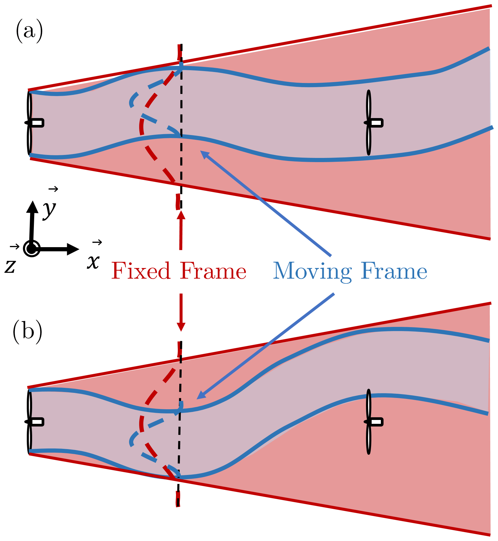
Figure 1Schematic of the wake meandering phenomenon. The mean (red) and instantaneous (blue) wake outlines are plotted at two different time steps: (a) the downstream turbine is inside the wake and (b) the downstream turbine is partially outside the wake. The mean velocity profiles in the fixed frame (red) and the moving frame (blue) are also plotted in dashed lines.
The evolution of the time-averaged wake may thus be considered the combination of two phenomena: on one hand the wake expansion and dissipation due to the turbulent diffusion and on the other hand the wake meandering due to large-scale forcing of the ABL. Most analytical models are calibrated directly in the frame of reference linked to the ground (called hereafter fixed frame of reference or FFOR) against reference data averaged over the meandering time period, and the wake widths are written as a function of the turbulence intensity (TI) upstream the turbine (Fuertes et al., 2018; Ishihara and Qian, 2018). This approach is straightforward, but the phenomena of meandering and turbulent mixing are not differentiated. The issue is that the atmospheric stability impacts meandering, leading to different time-averaged wake recoveries for a given upstream TI at hub height (Du et al., 2021). In order to accurately model wind turbine wakes in a non-neutral ABL, it is proposed to decouple the effect of meandering and the effect of wake expansion.
This can be achieved with the use of the moving frame of reference (MFOR), which is moving with the wake centre at each time step. The unsteady velocity field in the MFOR is thus equivalent to the velocity field that would be observed if there was no meandering. Due to the spreading caused by the meandering, the mean velocity deficit in the FFOR is weaker and wider compared to the mean velocity deficit in the MFOR (dashed red and blue profiles in Fig. 1). Conversely, the turbulence (not shown on the scheme) is stronger in the FFOR compared to the MFOR (Larsen et al., 2019). If a Cartesian coordinate system (x, y, z) is used for the streamwise, lateral and vertical coordinates respectively (see Fig. 1), the instantaneous velocity can be changed from one frame to another according to the relation
where subscripts MF and FF denote the velocity fields in the MFOR and FFOR respectively and yc(x,t) and zc(x,t) are the time series of the wake centre's coordinates at the downstream position x. The concept of MFOR was originally introduced for the dynamic wake meandering (DWM) model (Larsen et al., 2008) which aims at modelling the unsteady effects of meandering. The methodology to retrieve the velocity and turbulence fields in the FFOR with this model is briefly introduced here. In the DWM model, the wake in the MFOR is assumed to be steady and axisymmetric (Ainslie, 1988), and wake expansion and dissipation are assumed to be driven by turbulent mixing and the turbine's operating conditions. This steady wake is advected as a passive tracer by the largest eddies of the ABL to get the unsteady wake in the FFOR. If the unsteady FFOR velocity field is required, Eq. (1) is used with a steady, axisymmetric form in the MFOR, i.e. . If only the time-averaged field is needed, Eq. (1) reduces to a 2D convolution product (Keck et al., 2013b), denoted in the following. This is possible in the DWM framework, since UMF,dwm is considered to be steady, and thus the elements of the wake centre time series can be permuted without affecting the results of Eq. (1). It gives
where fc(y,z) is the probability density function (PDF) of the wake centre position, normalized such as . Here and in the following, the Reynolds decomposition is used to write any unsteady field X(t) as a sum of a mean and a fluctuating part: .
In the DWM, the total turbulence (defined as the temporal variance of the velocity field) in the FFOR in the wake can be computed as the sum of two components:
where ka is the rotor-added turbulence, mainly driven by the shear generated by the velocity deficit in the wake, and km is the meandering turbulence, generated by the lateral and vertical displacements of the wake. Similarly to Eq. (2), these two components can be written as (Keck et al., 2013b)
where kMF,dwm is the modelled turbulence in the MFOR, i.e. the turbulence that would be measured if there was no meandering. In the DWM model, an empirical scaling of UMF(y,z) with a factor kmt(y,z) is used to compute kMF,dwm (Madsen et al., 2010; Conti et al., 2021). Equation (6) is obtained by developing Eq. (5) and simplifying with Eq. (2). The added value of such an approach is that it allows writing the velocity and the turbulence in the FFOR as a function of the same fields in the MFOR, where they are presumed to be only dependent on the turbine's operating conditions, thus less complex and easier to model.
The objective of this work is to write the velocity and turbulence in the FFOR as a function of the velocity and turbulence in the MFOR and show the underlying DWM assumptions that neglect some terms. The importance of these missing terms for both velocity and turbulence is evaluated. The reference results come from large-eddy simulations (LESs) of an isolated wind turbine wake over flat terrain. Three cases of stability, approximately corresponding to the SWiFT benchmark (Doubrawa et al., 2020), are simulated using Meso-NH (Lac et al., 2018) with an actuator line method (ALM) (Joulin et al., 2020; Jézéquel et al., 2021).
This work is separated into two articles. In the present one, the breakdown of the velocity and turbulence is presented and applied to the LESs datasets. In the companion paper, the results are used to build a new analytical model for velocity and turbulence in the wake of a wind turbine. The first part of the present article is dedicated to the development of the velocity and turbulence breakdowns, i.e. the expression of the velocity and turbulence fields in the FFOR as a function of their counterparts in the MFOR. In the second part, the numerical framework is detailed: it describes the SWiFT cases, the LES code Meso-NH, the numerical set-up, the wake tracking algorithm and the limitations of these tools. In the third part, the LES datasets are used to quantify the error induced by the approximations necessary to write Eqs. 2 and 3. In the fourth part, some physical interpretations are proposed, the dependence of ka and km on atmospheric stability is studied and the shape of all the terms in the turbulence breakdown equation is described.
To lighten the mathematical formulations, the notation will be used to express the switch between FFOR and MFOR (Eq. 1). This operation can be interpreted as an unsteady translation of any field a by the meandering: the stronger the meandering, the more will be spread. It is important to note that a can be steady or unsteady, but is always unsteady. For any variables a and b, the following properties hold:
Properties (Eqs. 7 and 8) are obtained from the linearity of the translation operator. Property (Eq. 9) is trivial since is time-dependent and is not. Property (Eq. 10) can be demonstrated by defining fc as a sum of indicator functions and applying a Taylor development. Using the notation and applying the Reynolds decomposition to UMF allows one to re-write Eq. (1) as
The mean velocity in the FFOR can directly be deduced by applying the averaging operator to this equation:
From Eq. (10), it appears that term (I) is the convolution of with fc and can be viewed as a pure mean velocity term: it is null only if the mean velocity is null. Conversely, term (II) is here viewed as a cross term, because it can be null either if there is no meandering () or if there is no turbulence in the MFOR (). In the DWM model, UMF,dwm is steady, so and , thus Eqs. (2) and (12) are equivalent. The assumption of steady flow in the MFOR for analytical or DWM models is equivalent to the assumption that term (II) of Eq. (12) is negligible. Since is not necessarily true in real cases (nor in LESs, which are used here), this hypothesis must be verified, which is one of the objectives of the present work.
For the turbulence equation, one can write from Eqs. (11) and (12)
The total turbulence in the FFOR can then be written as a function of the preceding quantities:
Term (III), also written km in the following for consistency with the literature (Keck et al., 2013b; Conti et al., 2021), is the turbulence purely induced by meandering: in the case of a meandering steady wake, i.e. , Eq. (15) reduces to this term only. Note that km is the variance of . In the DWM model, the wake in the MFOR is steady, but a rotor-added turbulence term is added to model the small-scale turbulence that exists in the MFOR in real cases. This rotor-added turbulence can be calibrated from the MFOR turbulence in reference data i.e. term (IV) of Eq. (15). It is the turbulence purely induced by the rotor: in the absence of meandering (), the equation reduces to this term only, also written ka in the following. It is also denoted ka for consistence with the literature.
Through Eq. (3), it is assumed in the DWM that the wake turbulence is separated between two terms: one purely induced by the meandering – km,dwm, related to term (III) – and the other purely induced by the rotor – ka,dwm, related to term (IV). The analysis presented above shows that three cross terms are neglected under this assumption. Term (V) is the covariance of and , term (VI) is the remaining of when subtracting the rotor-added turbulence in the FFOR (it can be viewed as the varying part of the MFOR turbulence), and term (VII) is the square of term (II). It is a dissipation term as it is always negative. Like term (II), these are cross terms, since they are equal to zero if either the turbulence in the MFOR or the meandering is null.
Similarly to the velocity field, Eq. (15) shows that when calibrating a DWM-type model against realistic data (measurement or high-fidelity simulation, denoted subscript “cal”), if it is assumed that and , then there will be three missing terms: (V), (VI) and (VII). Like term (II) for the velocity, these terms cannot be computed directly from a steady model of the velocity in the DWM so similarly to term (IV), they must be modelled differently.
It has thus been shown in this section that the mean velocity turbulence fields in the FFOR can be broken down into two types of terms: pure terms – (I), (III) and (IV) – and cross terms – (II), (V), (VI) and (VII). In models where the wake is considered steady in the MFOR and advected as a passive tracer (such as the DWM or the model developed in the companion paper), the pure terms are modelled but the cross terms are implicitly neglected. The error induced by this assumption is verified in this work with LESs.
3.1 The SWiFT benchmark
The breakdowns of the mean velocity and turbulence fields in the FFOR described in Sect. 2 are applied to three LESs cases. These datasets, already presented in Jézéquel et al. (2022), are the result of simulations that reproduce the SWiFT benchmark (Doubrawa et al., 2020) with the LES code Meso-NH (Lac et al., 2018). The simulated turbine is a modified version of the Vestas V27: it is a three-bladed rotor with a diameter of D=27 m and a hub height of 32.1 m. The orography of the terrain is neglected, and three cases of stability are simulated: near-neutral, unstable and strongly stable. The simulations are classified with the Monin–Obukhov length:
where is the friction velocity, is the turbulent potential temperature flux and θ is the potential temperature. All these variables are computed at z=10 m above the ground. κ and g are the Von Kármán and earth gravity constants. For the neutral, unstable and stable cases, the stability parameters at z=10 m are respectively , −0.16, 0.60}, the inflow velocities at hub height are Uh={8.4, 6.2, 4.7} m s−1, the inflow streamwise turbulence intensities at hub height are 11.2, 12.3, 3.7} % (kx is the variance of Ux) and the thrust coefficients are CT={0.79, 0.81, 0.82}.
3.2 The Meso-NH LES solver
MESOscale Non-Hydrostatic (Meso-NH) is a finite volume and finite difference open-source research code for ABL simulations developed by the Centre National de Recherches Météorologiques and the Laboratoire d'Aérologie. The model is described in detail in Lafore et al. (1998) and Lac et al. (2018). The filtered Navier–Stokes and energy conservation equations are resolved on an Arakawa C-grid. The unknowns of the system are the velocities (Ux, Uy and Uz) and the potential temperature θ. A constant density profile ρ(z) is imposed, except for the buoyancy term (anelastic assumption), and the vertical velocity is driven by the vertical pressure gradient and the gravity (non-hydrostatic set of equations). The Coriolis force is added to the momentum equation, as well as a large-scale forcing term, which is imposed by the user through a 2D geostrophic wind Ug.
The turbulence closure is of the order 1.5: an additional equation is introduced for the subgrid kinetic energy esgs, and the other subgrid terms are modelled as functions of the resolved quantities, esgs and a mixing length Lm (Cuxart et al., 2000). The mixing length is related to the grid size and stratification through the Deardorff formulation (Deardorff, 1980). This set of equations is discretized spatially with a fourth-order centred scheme and temporally with a fourth-order Runge–Kutta scheme.
To model the wind turbine, the ALM is used, following Sørensen and Shen (2002). This method has been implemented in Meso-NH, validated against the New MEXICO wind tunnel experiments (Joulin et al., 2020) and the in situ measurements and LESs codes of the SWiFT benchmark (Jézéquel et al., 2021). A grid nesting technique allows the coupling of two or more computational domains of different sizes, temporal and spatial resolutions (Stein et al., 2000). The velocity field of a father domain Di is interpolated to the boundaries of a son domain Di+1. Hence, the resolution can be brought below the metre (necessary here to have 30 mesh points per blade as recommended in Troldborg, 2009), while still taking into account the large-scale behaviour of the ABL.
3.3 Numerical parameters
The numerical parameters used for the three simulations are presented in Table 1 for the different domains of the grid nesting. The size of the horizontal mesh depends on the domain Di, but in Meso-NH the vertical mesh is the same for every domain. In the induction and the wake regions, the vertical discretization ΔZ is set to have isotropic cells in the most refined domain i.e. D4 in the neutral and unstable cases and D2 in the stable case. The bottom boundary condition is determined by the subgrid heat and momentum fluxes. The heat flux is prescribed and governs the evolution of θ in the middle of the first cell, along with other resolved processes such as advection. The momentum flux at the surface is computed according to the Monin–Obukhov similarity laws, depending on the roughness length, wind at the middle of the first grid mesh and heat flux. It is used to compute the velocity at the first grid mesh.
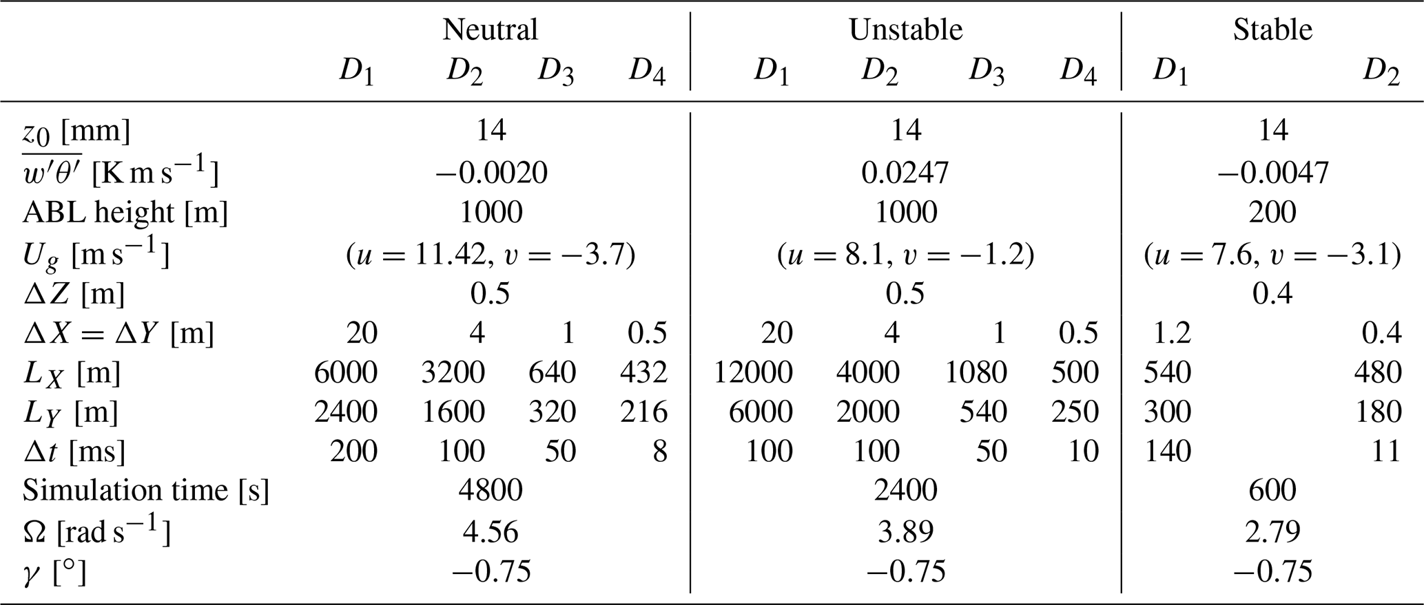
The flow field is initialized with a constant-velocity profile equal to the geostrophic wind. A constant-temperature profile is set up to an arbitrarily defined ABL height, capped by an inversion region of 5 K over a depth of 50 m. The geostrophic wind, ABL height, surface roughness z0 and kinematic vertical heat flux are chosen to be as close as possible to the SWiFT measurements in terms of velocity, wind direction, turbulent kinetic energy (TKE) and stability parameter.
In the first domain D1, the boundary conditions are cyclic to let the turbulence establish, with dimensions LX and LY larger than the largest eddies of the flow. In a stable ABL, these eddies are smaller, which is why a smaller domain D1 is suited, and inversely for the unstable case. After an initialization of turbulence in domain D1, the nested domains (D2, D3 and D4) are successively created. In each nested domain Di, a region in which the turbulent flow adapts to the finer resolution (in brown in Fig. 2) appears near the inflow. The next domain Di+1 must avoid it, so a spectral analysis (not shown here) has been carried out to measure the end of this perturbed region. The time step in every domain is driven by the Courant–Friedrichs–Lewy number condition, except for the finest domain, where it is equal to the time needed for the tip of the blades to cross one cell.
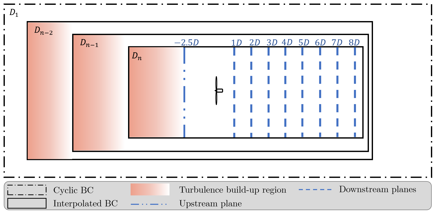
The size of the domain of interest (D4 in the neutral and unstable case and D2 in the stable case) is set to compute the wake up to 8 D downstream of the turbine. This choice has been made to keep reasonable simulation times for the LES and a high degree of confidence in the wake tracking algorithm. However, the wake is not dissipated at this position, and the present work could be completed with a study where the wake is computed further downstream, e.g. at .
The ALM is activated once the flow is established in the most refined domain, and after a 10 min spin-up to let the wake flow establish, the instantaneous velocity is extracted at one plane upwind of the turbine and several planes downwind, according to Fig. 2. Note that the simulation time is case-dependent: 80, 40 and 10 min for the neutral, unstable and stable cases respectively.
The rotational velocity of the wind turbine Ω and pitch of the blades γ are set constant to a value interpolated in the controller table of the turbine with the upstream velocity at hub height Uh, and a simple implementation of the nacelle and the tower is used (corresponding to Stevens et al., 2018).
3.4 Wake tracking
The wake meandering is characterized by the time series of the wake centre coordinates yc(x,t) and zc(x,t). Even though it is a very handy concept from a theoretical point of view, defining the centre of the wake or even its borders is difficult, especially when the wake is developing inside a turbulent boundary layer. Indeed, the turbulent structures can move, twist or even split the wake, and low-velocity eddies can be mistaken for the wake.
To determine the wake centre at each time step, an algorithm based on the conservation of momentum in the wake is used (Quon et al., 2020). First, the 2D velocity and momentum deficits are computed at each time step and for each downstream plane:
where U is the streamwise velocity in the simulation and Uref is the streamwise velocity in a reference simulation, i.e. a simulation without the wind turbine but with the same inflow and boundary conditions. This operation allows removing the atmospheric shear and low-velocity eddies of the ABL that can be mistaken with the wake. A moving-average operator is applied on the velocity field with a window of seven frames (i.e. 7 s). This window size is chosen to smooth the data and facilitate the wake tracking while not impacting significantly the resulting time series of the wake centre's coordinates. The wake outline is then defined as the best fit of isoline that encloses a surface S such as
where ρ is the density of the fluid and is the mean thrust. The wake centre is then computed as the velocity deficit centroïd of S. An illustration of this algorithm at for an arbitrary time step is given in Fig. 3. This post-processing is performed with the python post-processing tool SAMWICH (Quon et al., 2020) where this algorithm is referenced as Constant Flux or CstFlux. This algorithm has been chosen for its high success rate and physically consistent fields in the MFOR (Jézéquel et al., 2022). Finally, several extreme values of yc and zc are considered outliers (in the worst case it concerns about 5 % of the frames) and manually removed from both the FFOR and MFOR datasets.
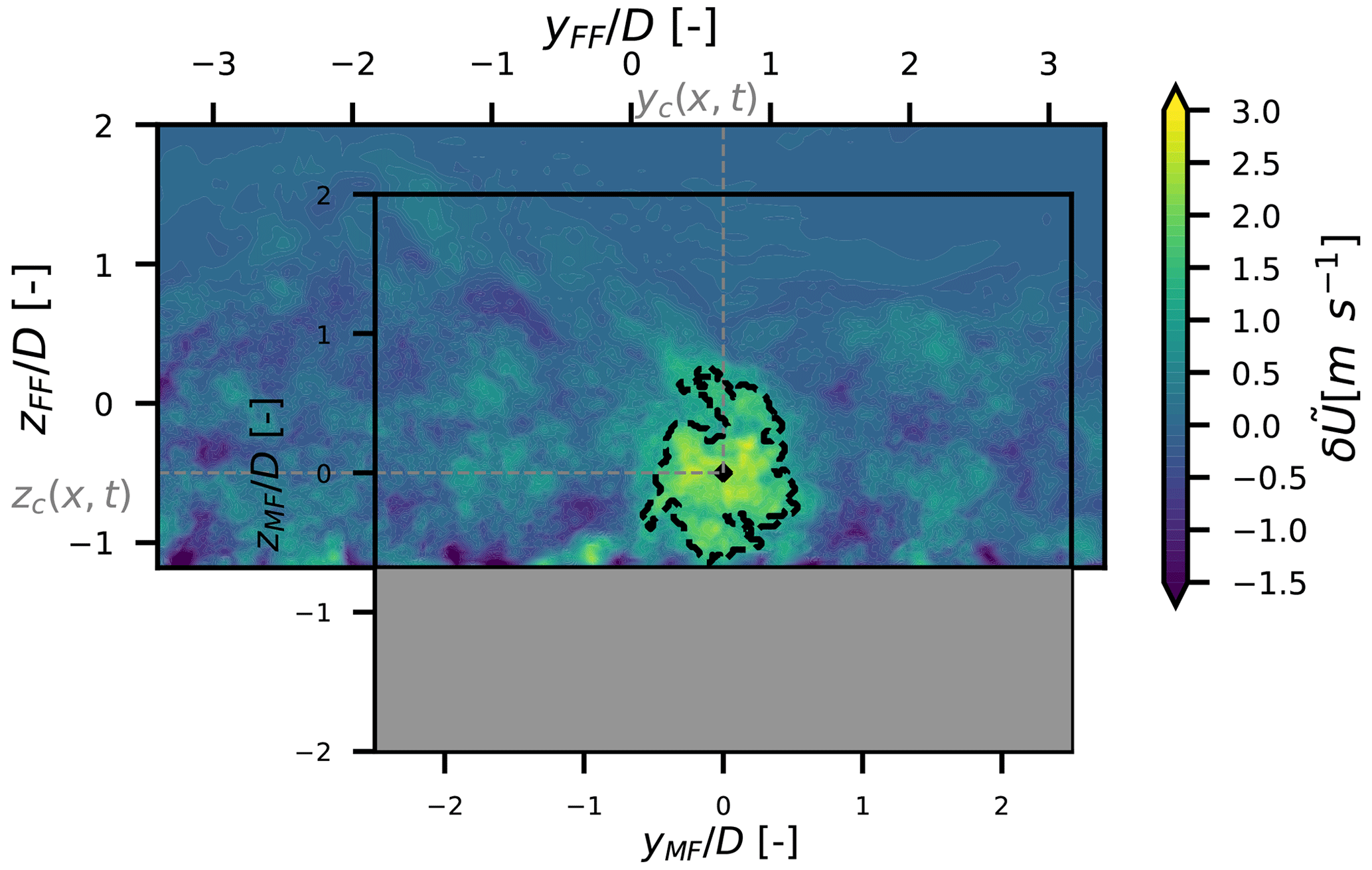
Figure 3Result of the wake tracking at an arbitrary time step at x=6 D downstream. The detected isocontour is in the dashed line and the detected wake centre is represented by a diamond.
3.5 Limitations
To compute terms (I) to (VII) of Eqs. (12) and (15), it is needed to start from the unsteady field UMF and apply the Reynolds decomposition and operator i.e. reverse Eq. (1). To avoid losing any data, one should compute the MFOR on a grid spanning from to and similarly in the vertical direction. For strong meandering cases, it would result in a very large grid that would be computationally costly to manipulate. It has thus been decided to restrain the MFOR to . Consequently, some data are missing in the MFOR, leading to unavoidable small differences between the left- and right-hand sides of Eqs. (12) and (15).
Given that the ground is located around D, the velocity field UMF at is undefined since it is located under the ground (the grey region in Fig. 3), so this part of the velocity field is ignored when computing the mean and standard deviation of the velocity in the MFOR. Consequently, the statistics (mean and variance) near the ground in the MFOR are computed with fewer samples than those at higher positions.
The wake tracking and the computation of each term of Eqs. (12) and (15) are a costly post-processing, in terms of computational resources and memory. Given the relatively low time step imposed by the ALM it was not feasible to apply this algorithm to every LES time step, so a sampling frequency of 1 Hz has been chosen to store the output velocity field of Meso-NH. This means that all the variations of the wind velocity at frequencies higher than 1 Hz are not taken into account in this work, nor is the subgrid turbulence. Since subgrid turbulence is a prognostic variable in the 1.5-order closure used in Meso-NH, one can compute the ratio between subgrid and total turbulence. It is between 1 % and 5 % in the neutral and unstable case but can reach more than 20 % in the stable case. This highlights the difficulty of simulating strongly stratified ABL, but our results have been successfully compared to the SWiFT benchmark (Jézéquel et al., 2021), so they will be used nonetheless.
The error induced by the choice of the 1 Hz sampling has been estimated with a 95 % confidence interval and discussed in Appendix A for the MFOR turbulence and all the terms of Eq. (15). In short, the chosen sampling frequency of 1 Hz is sufficient for the neutral and unstable cases. In the stable case, due to the higher share of small-scale turbulence, the 95 % interval is large, indicating that a higher sampling frequency would improve the accuracy of the LES.
Due to numerical limitations, the duration of the simulations was constrained to 80, 40 and 10 min (see Table 1). To estimate the statistical convergence, each of these segments is divided in two, and the difference between the two sub-segments and the full simulation is assessed in Appendix A. It appears that the stable and the neutral simulations would barely benefit from an extension of their duration, whereas the unstable simulation seems to change significantly between the two sub-segments of 20 min. This is particularly true for terms (V) and (VI) of the turbulence breakdown equation (Eq. 15).
Finally, the streamwise component of the velocity is computed in the following, in both MFOR and FFOR. In all the following, the mean streamwise component of the velocity will be noted Ux, and the streamwise turbulence will be used to differentiate from the total TKE.
Once the Meso-NH simulations are performed, Ux and kx in the FFOR are directly computed as the mean and variance of the unsteady streamwise velocity field. The wake tracking algorithm described in Sect. 3.4 is applied to get the unsteady streamwise velocity field in the MFOR. The Reynolds decomposition and meandering operator can then be applied to get the values of terms (I) and (II) of Eq. (12) and terms (III)–(VII) of Eq. (15).
The objective of this section is to quantify the importance of each term and to estimate the error induced by neglecting the cross terms in the velocity and turbulence breakdowns, for instance in the DWM model or in the model developed in the companion paper. The focus is on the neutral case to keep a concise section. The normalized root mean square error (RMSE) indicator (Eq. 20) is used to quantify different levels of approximation with the actual results in the FFOR:
where α is the reference value (directly extracted from Meso-NH), αp is the predicted value, N is the number of samples and αmax−αmin is the range of α over those samples. When the RMSE is computed on a Y–Z plane, only the truncated plane , is used to avoid edge effects and then N denotes the number of mesh points in this plane.
4.1 Velocity field
In Eq. (12), the velocity is separated into terms (I) and (II). The vertical profiles of these terms for the neutral case are plotted in Fig. 4 for several downstream positions. Term (I), which is the convolution of the velocity in the MFOR with the distribution of wake centre position, actually fits very well with the velocity in the FFOR. Small differences only appear in the near wake. Term (II) is plotted on a secondary axis (displayed at the top of the figure) to show that it has a negligible value: less than 0.3 m s−1 in absolute value, i.e. less than 4 %. In the stable case it is even more negligible but in the unstable case (both are not shown here for conciseness), it takes slightly larger values of about 0.5 m s−1 i.e. 10 % at the wake centreline in the near wake. As it can be seen at the bottom of the profiles, the main role of this term in the far wake is to reproduce the shear near the ground that is missing in the MFOR, and thus not present in term (I).
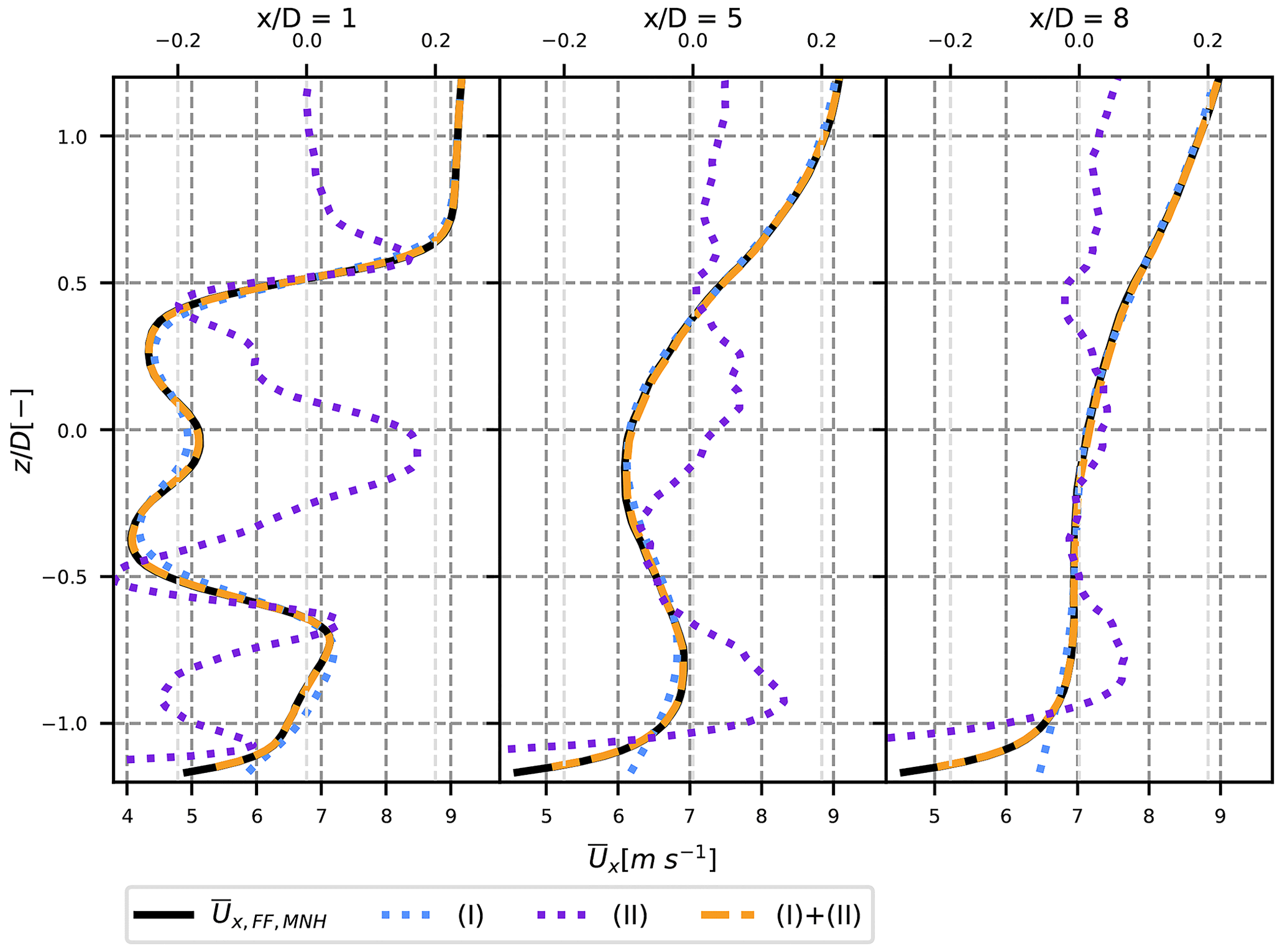
Figure 4Contribution of terms (I) and (II) from Eq. (12) to the velocity in the wake of the neutral case, compared to the velocity in the FFOR. Term (II) is plotted on a different scale (top axis).
From this first observation, it seems acceptable to neglect term (II). The effect of this assumption can also be measured with a global variable. It has been chosen to investigate the error induced by neglecting term (II) on the available power, since predicting the power output of a farm is a direct application of analytical models. The available power is here defined as
where S is the surface of a virtual wind turbine located at position x behind the wake-emitting turbine, with hub height at the same position: y=0 and z=0 coordinates. This quantity is computed for (I) and (I) + (II) at each available position downstream of the wind turbine and compared to the same quantity directly computed on the Meso-NH field in the FFOR Pa,FF.
From Fig. 5, it appears that neglecting term (II) in the neutral case leads to a slight overestimation of the available power in the near wake of the wind turbine. The estimation is however fairly good, especially for a wind turbine located further than 3D downstream where the overestimation drops below 2 %. The relative error is larger in the unstable case, going from +5 % to −6 % between 1D and 8D downstream. This negative value shows an underestimation of the mean velocity by term (I) in the far wake. One can note that, at these positions, the tracking algorithm of the unstable case is less reliable, so it could be the source of the error. In such a case, approximating with (I) would be correct and the error would come from our methodology. In the stable case, the error is much lower: less than 0.3 %. Further study should be used to determine whether the growing importance of term (II) in the unstable case comes from post-processing errors or actual physical phenomena. Overall, if the velocity near the ground is not of interest, approximating the FFOR velocity as term (I) alone as it is done in the DWM can thus be acceptable given the low error on estimated power. This is especially relevant since term (II) seems very chaotic (see Fig. 4) and thus hard to model.
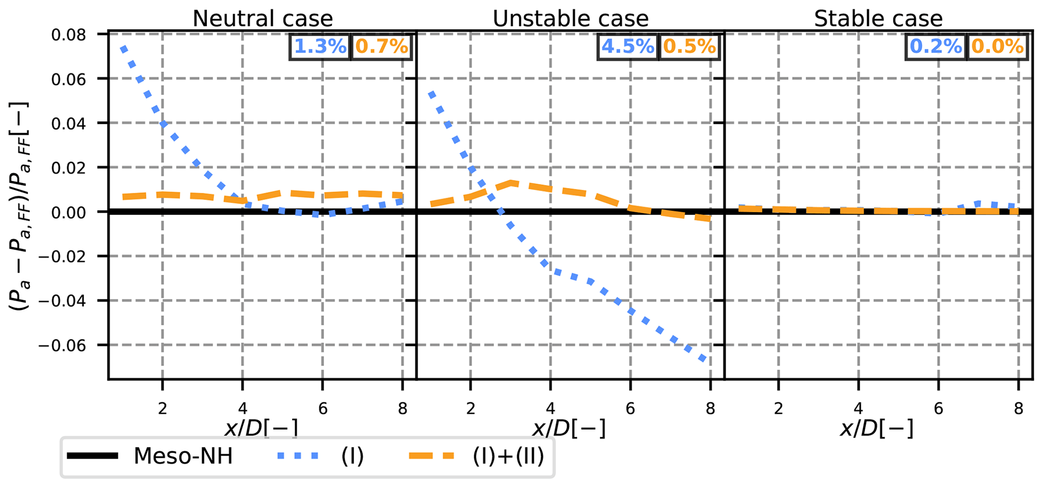
Figure 5Available power predicted by (I) (blue) and (I) + (II) (yellow) for the three simulation cases. The value is normalized with the results in the FFOR (black line). The RMSE of Pa averaged over all the x positions is displayed at the top in the corresponding colour.
4.2 Turbulence field
The same study is performed for the turbulence field in the wind turbine wake. The vertical turbulence profiles for the neutral case are plotted for different levels of approximation, at different positions downstream in Fig. 6. In the DWM model, only the meandering (III) and rotor-added turbulence (IV) terms are retained. This corresponds to the blue curve: despite an overall good order of magnitude, it can be seen that the vertical asymmetry is not sufficiently pronounced, leading to an underestimated value of kx at the top tip and overestimated value at the bottom tip. This issue, especially true in the near wake, has already been observed in another work that used an equation similar to Eq. (15) (Conti et al., 2021) to compare the DWM results to in situ measurements. If horizontal profiles at hub height are plotted instead (shown in the companion paper), the results are much better and the DWM approximation seems suitable, for not only the neutral but also the unstable and stable cases.
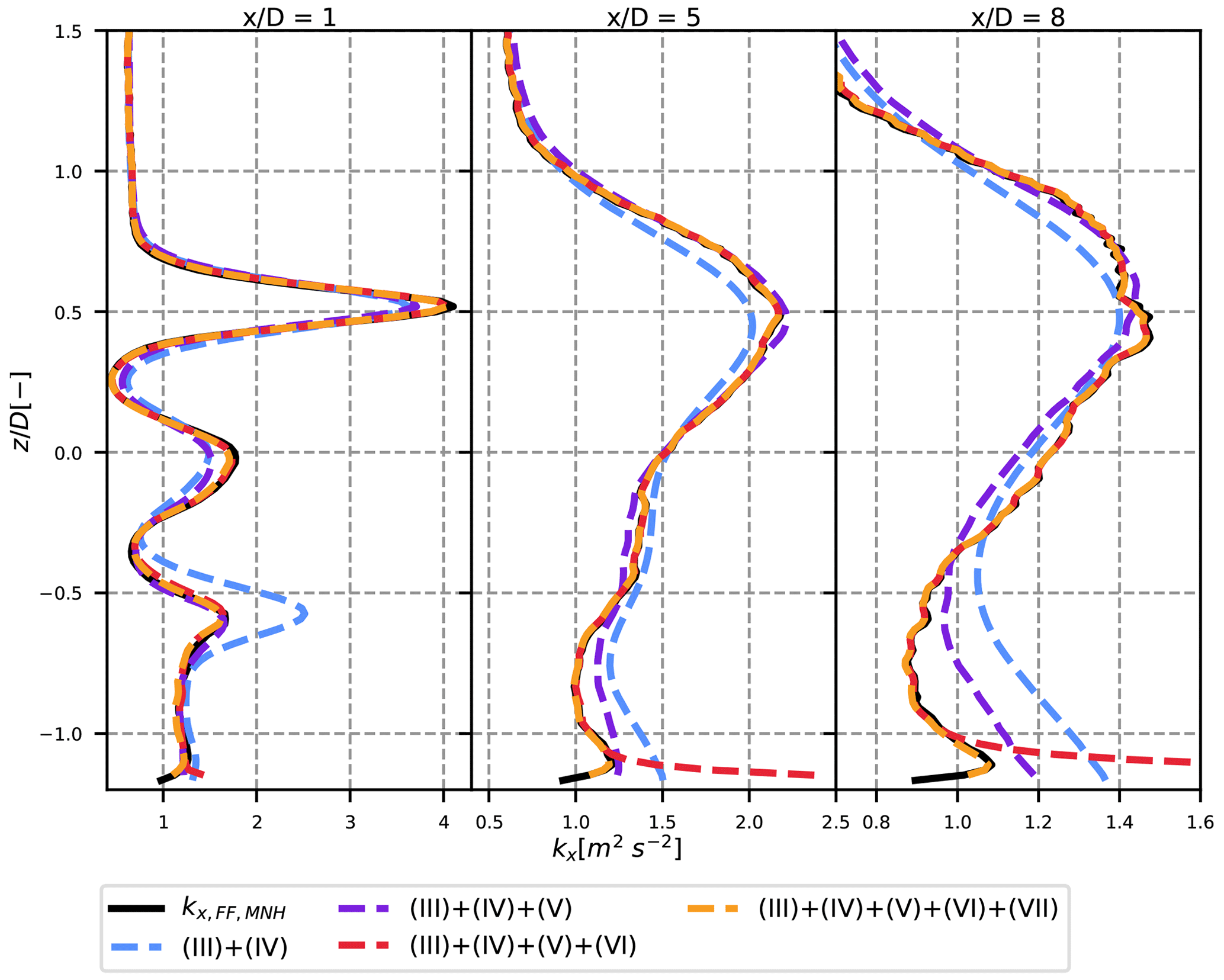
Figure 6Streamwise turbulence profiles in the wake of the wind turbine for different levels of approximation. Neutral case at three positions downstream (1, 5 and 8 D).
Adding the covariance term (V) along with terms (III) and (IV) (purple curve in Fig. 6) corrects for most of the vertical asymmetry of the turbulence profiles and leads to a rather good estimation of the maximum turbulence values at the top and bottom tips. The main effect of adding term (VI) (red curve) is to take the spatial small-scale variations into account, bringing the total kx even closer to its reference value. As pointed out previously, term (VII) is the square of term (II): like the latter, it mainly has an effect near the ground but is otherwise negligible.
To quantify more clearly these differences, the maximum axial turbulence is studied. It is computed directly in the FFOR () and for different levels of approximation from Eq. (15). Their evolution with the downstream distance is plotted in Fig. 7, normalized by , and the same colour convention as in Fig. 6 is used.
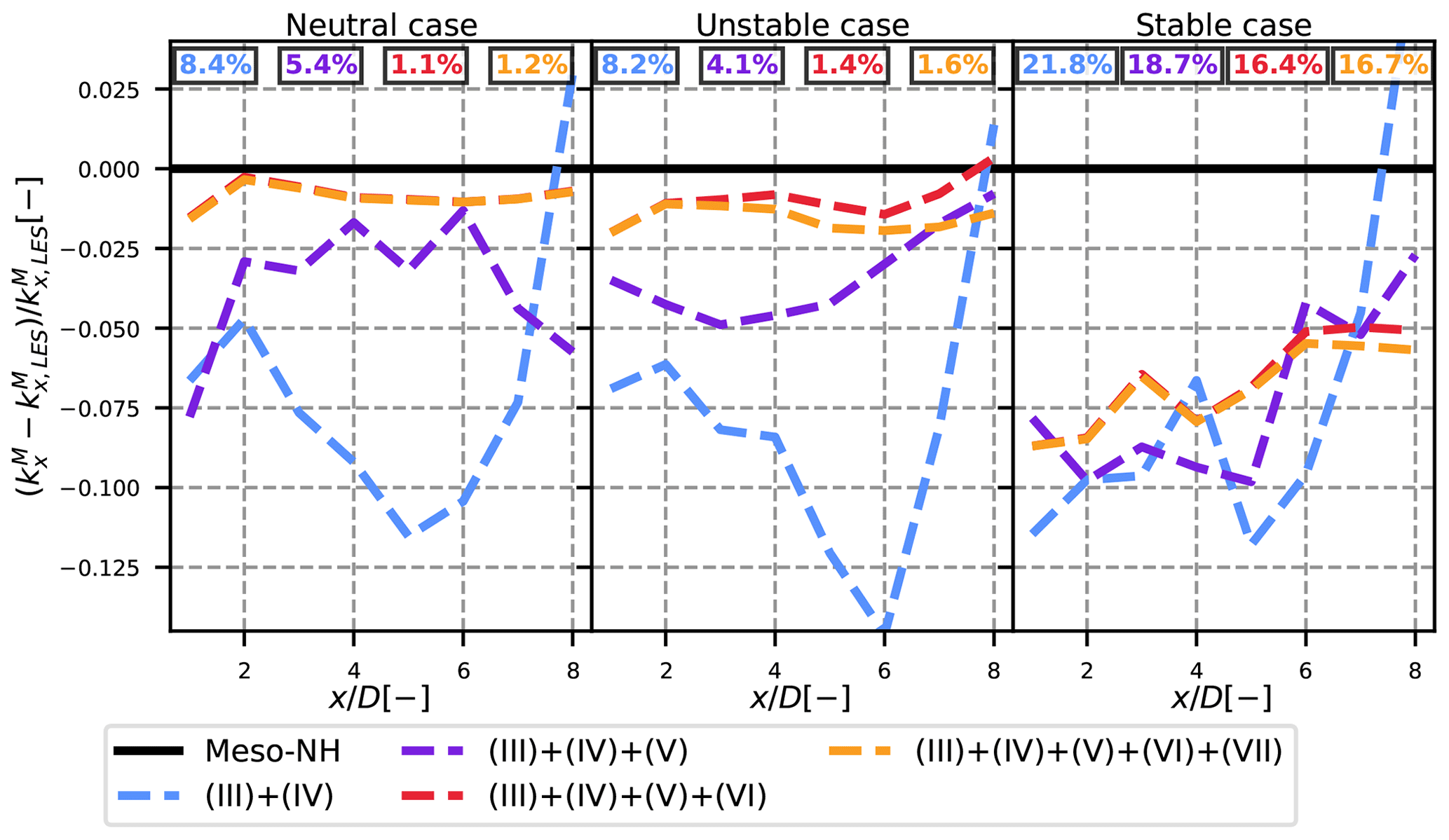
Figure 7Normalized maximum turbulence in the wake for different levels of approximation as a function of the downstream position for the three simulation cases. The RMSE of averaged over all the x positions is displayed at the top in the corresponding colour.
In the neutral case, neglecting the cross terms leads to an underestimation of about 6 % to 12 % of the maximum turbulence in the wake. In the far wake (beyond ) the error decreases, but this is a numerical artefact: due to edge effects, large kx values are observed near the ground, and thus the maximum kx is detected at this location instead of at the top tip. Adding the covariance term (V) allows us to bring this number down between 2 % and 6 %, and adding term (VI) to this total leads to a negligible underestimation (around 1 %). Term (VII) has a negligible effect on the maximum turbulence (orange and red curves are superimposed). The remaining gap is attributed to the error reconstruction due to the MFOR not being large enough (see Sect. 3.5).
For the unstable case, the same orders of magnitude are observed for the different kx approximations: adding the convolution term (V) reduces the relative underestimation of by at least half, and using (III) + (IV) + (V) + (VI) leads to a fairly good approximation. In the stable case, however, the error remains between 5 % and 10 %, independently of the level of approximation. This is because despite an improvement over the whole profile, the maximum is not well captured (figure not shown here for brevity). The relatively high error percentage is attributed to low absolute values. Indeed, the error is of the order of magnitude of 0.04 m2 s−2, which is in the end similar to the other cases. Term (VII) is negligible in every case.
It has been shown in this section that neglecting term (II) as in the DWM model or in the companion paper leads to a rather accurate velocity deficit in the wake and a reasonable estimation of the available power (less than 2 % overestimation) for a wind turbine inside the wake, as long as it is positioned beyond . For the turbulence breakdown, term (VII) is also negligible, but the vertical turbulence profiles are prone to errors when term (VI) and more importantly term (V) are not taken into account, leading to an underestimation of the maximum turbulence in the wake. It is now needed to compare the shapes and the relative magnitude of these terms before modelling them.
In this section, the turbulence fields in the wake of the wind turbine are compared for the three cases of stability. The influence of atmospheric stability on each term of Eq. (15) is highlighted, and the shape of these terms in the Y–Z plane is analysed.
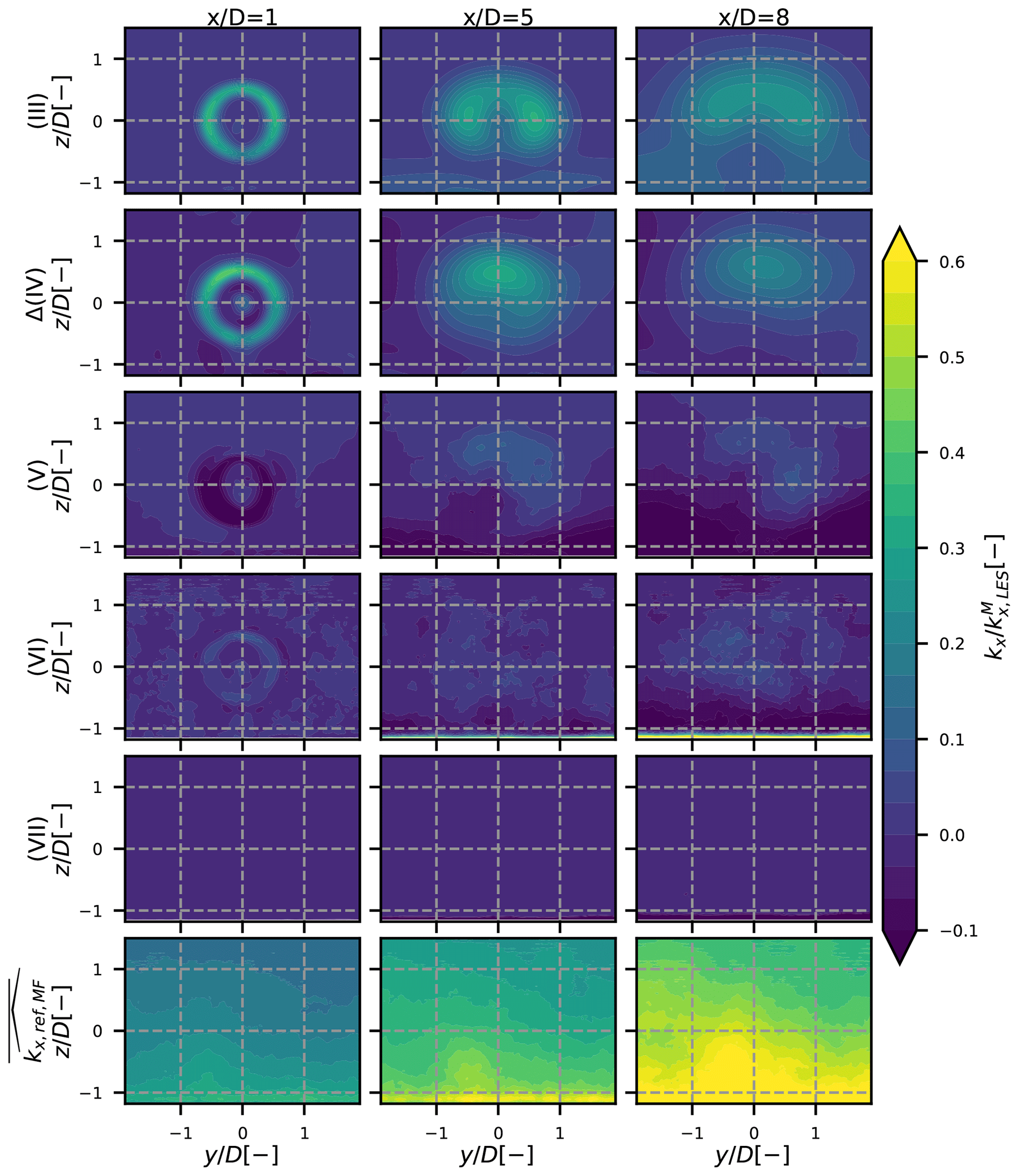
Figure 82D maps of the different terms in Eq. (15) for the neutral case. The different rows stand for the different terms, and each column is a different position: 1, 5 and 8 D downstream. The values are scaled by the maximum kx in the FFOR at the given x position.
5.1 Shape and values of the terms
The values of each term of Eq. (15) at different Y–Z planes downstream of the turbine in the FFOR are displayed in Figs. 8–10 for the neutral, unstable and stable cases respectively. The terms are normalized by the maximum total turbulence in the FFOR in the 2D plane, so the scale is approximately the fraction of the total axial turbulence represented by each term. Term (IV) contains both the rotor-added turbulence and the inflow turbulence, the latter of which is removed by subtracting the reference turbulence field in the MFOR taken from the reference simulation (i.e. the same simulation without the turbine; see Sect. 3.4) at the same location as the turbulence field with the wind turbine. In the MFOR the rotor-added axial turbulence is thus defined as the difference of axial turbulence between the simulation with and without the wind turbine:
Note that the yc(t) and zc(t) computed in the simulation with a turbine are re-used to compute the reference MFOR field and to apply operator to the reference data. The rotor-added turbulence can then be defined in the FFOR as
For the neutral case of stability (Fig. 8), the meandering (III) and rotor-added Δ(IV) terms have similar orders of magnitude and contain most of the total wake added turbulence. However, the covariance term (V) cannot be ignored as it rebalances the total turbulence of about ±10 % between the top and bottom regions of the wake, as it has been seen in Fig. 6. Term (VI) also shows non-negligible values, in particular in the far wake where it progressively takes values closer to the other terms, but the shape of this term seems to be randomly distributed (contrarily to term (V) which is located in the rotor-swept area). As stated in Sect. 4, term (VII) is negligible, except near the ground.
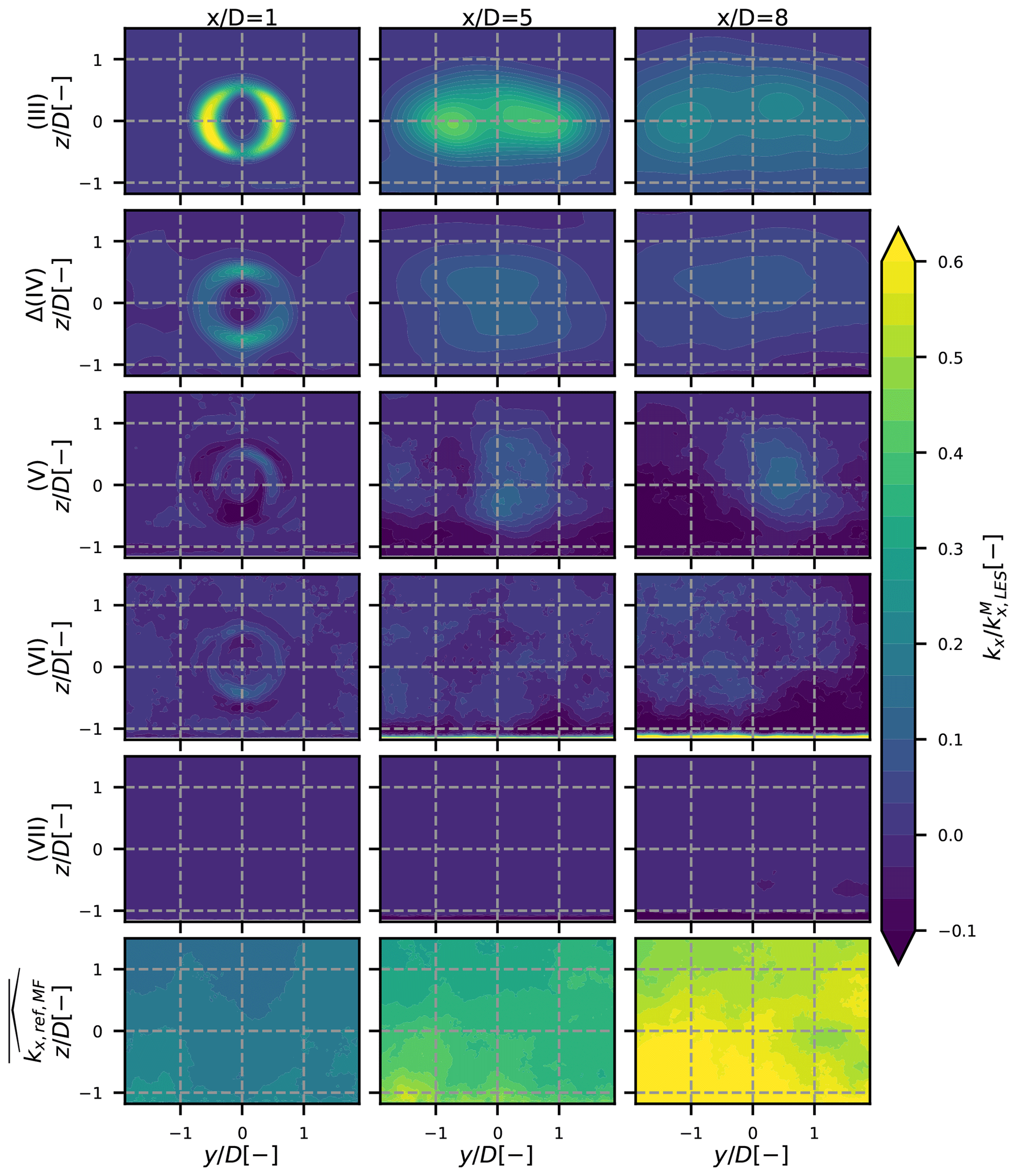
Figure 9 has been plotted similarly to Fig. 8 with the results of the unstable case. The meandering term (III) is dominant over the others, and the wake is quickly dissipating. The rotor-added turbulence has lower relative values and is more spread than in the neutral case. This is due to larger meandering in the unstable case i.e. a PDF fc with larger values at the edge and thus more spreading caused by the operator . The covariance term is also not negligible: here it takes values between terms Δ(IV) and (III) in the far wake. In this case, term (V) is symmetric about the vertical axis instead of the horizontal one. Term (VI) shows lower values that seem to be randomly distributed as in the neutral case. Term (VII) is still negligible.
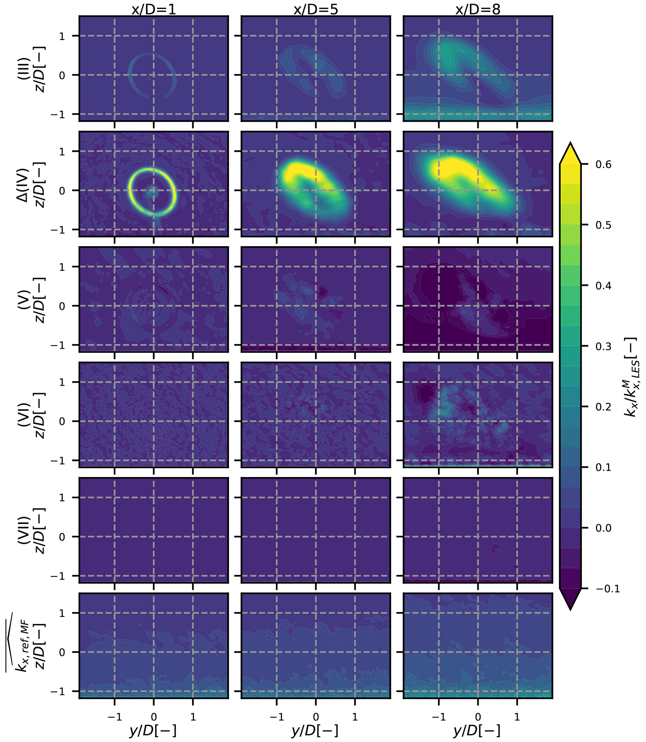
In the stable case (Fig. 10), it is the rotor-added turbulence that is largely predominant over the meandering and even the upstream terms. This can be explained by the fact that meandering is very weak, so term (III) is low, term (IV) is almost not spread by the convolution with fc, and the wake is barely dissipated, even at . The covariance term is here negligible except at where it slightly reduces the peak of turbulence at the top-left end of the wake. Term (VI) and particularly term (VII) are negligible in front of term (IV). The shape of all these terms is skewed due to the strong veer present in the stable ABL.
The reference turbulence in the FFOR is also plotted in the last line of Figs. 8–10 to quantify how the wake turbulence is going back to its unperturbed value: the closer is to 1, the more dissipated is the wake. At in the unstable case (Fig. 9), the reference turbulence in the FFOR represents the main part of the total turbulence which means that the wake is almost dissipated. Conversely, in the stable case (Fig. 10), the reference turbulence in the FFOR is negligible, compared to the other terms, showing that the wake is much less dissipated than in the other cases.
For all cases, the non-zero values of each term in the near wake (first column of every figure) are mostly distributed around the tip of the blades. For pure terms (III) and (IV), they are spatially smoothly distributed at and . For cross terms (V) and (VI) and (VII), the non-zero values at these positions are chaotically distributed spatially and thus harder to interpret due to a lot of small-scale variations. A statistical averaging of every term over several simulations could provide data with better spatial coherence, and the different terms would thus be easier to interpret. To do so, longer simulations with similar mean upstream conditions are needed.
5.2 Physical interpretation
Term (III) or km is the pure meandering term. For a fixed point downstream of the turbine, the meandering of the wake induces an alternation between low velocity (when the point is inside the wake) and high velocity (when it is outside the wake), i.e. variance in the unsteady velocity field, which is the definition of turbulence. km thus increases with the velocity deficit in the MFOR and with the amount of meandering. The former decreases with x whereas the latter increases with x, often linearly (Keck et al., 2013a; Ning and Wan, 2019; Brugger et al., 2022). These two contradictory trends lead km to be strong and very localized at the tip of the blades in the near wake and to be progressively smeared as the wake travels downstream. Since the meandering is stronger in the horizontal direction than in the vertical direction, and the velocity deficit is approximately axisymmetric (see the companion paper for more details), the highest values of km in the horizontal plane are stronger than in the vertical plane.
At a fixed x, the maximum values of km are localized near the tip of the blades in the near wake and are gradually spread as the wake travels downstream. The maximum added TI induced by term (III) (i.e. square root of the maximum value, normalized by the upstream velocity at hub height) is plotted in dashed lines as a function of in Fig. 11. As seen in Figs. 8–10, the meandering-induced turbulence is inversely related to the atmospheric stability, but this term also decreases faster in the unstable case, likely because the stronger the meandering, the more dissipated is the wake. Consequently, at the unstable and neutral added TI due to the meandering are almost identical, and the curves would probably switch at larger x. In the stable case, the velocity profile is barely dissipated up to , and the meandering starts to take consequent values at , which results in an increase of the added turbulence due to meandering starting from . One can predict that beyond , a maximum value is reached, followed by a shape similar to the unstable and neutral case.
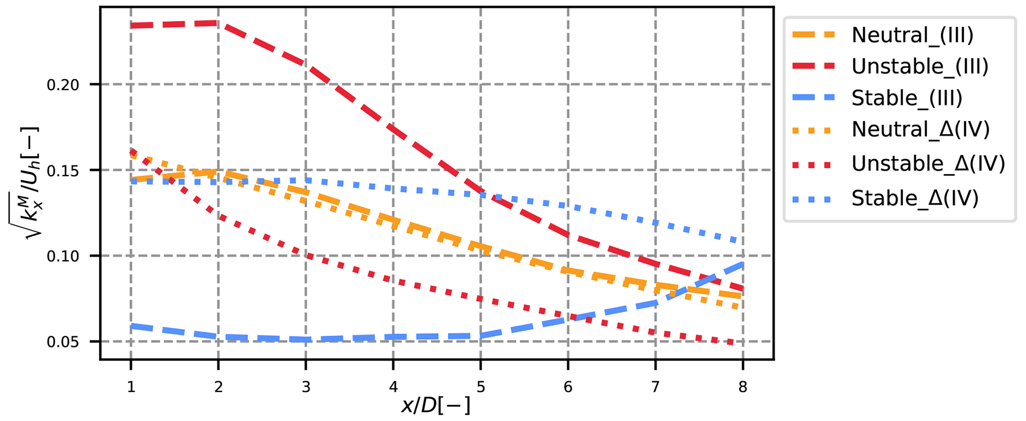
Figure 11Evolution of the maximum value of terms (III) and Δ(IV) with x, normalized by the velocity at hub height.
Term Δ(IV) noted ka for “rotor-added turbulence” is the turbulence that would exist in the wake of the turbine if there was no meandering. This turbulence is mainly due to the velocity gradient in the MFOR, localized at the edge of the wake. It is affected by the shear of the ABL, leading to a stronger gradient near the top tip and thus stronger rotor-added turbulence. This is particularly visible in the neutral and stable cases, where the atmospheric shear is significant. Similarly to the velocity field, this added turbulence is spread by meandering, more strongly in the lateral direction than in the vertical one, leading in the unstable case to lower values of ka at the side tips than the bottom tip despite the atmospheric shear being stronger at the side. This spreading of meandering also induces lower values of maximum added turbulence for lower stability cases (dotted lines in Fig. 11). To analyse the shape of the rotor-added turbulence before the spreading due to meandering, one needs to look at the values of ka in the MFOR. It is normalized with the hub height velocity to give the added TI in the MFOR:
Equation (24) allows identifying in which region the turbulence in the MFOR is lower than the unperturbed turbulence, without leading to undefined values of the square root. The values of ΔTIMF in the three cases of stability are plotted in Fig. 12 at different positions downstream.
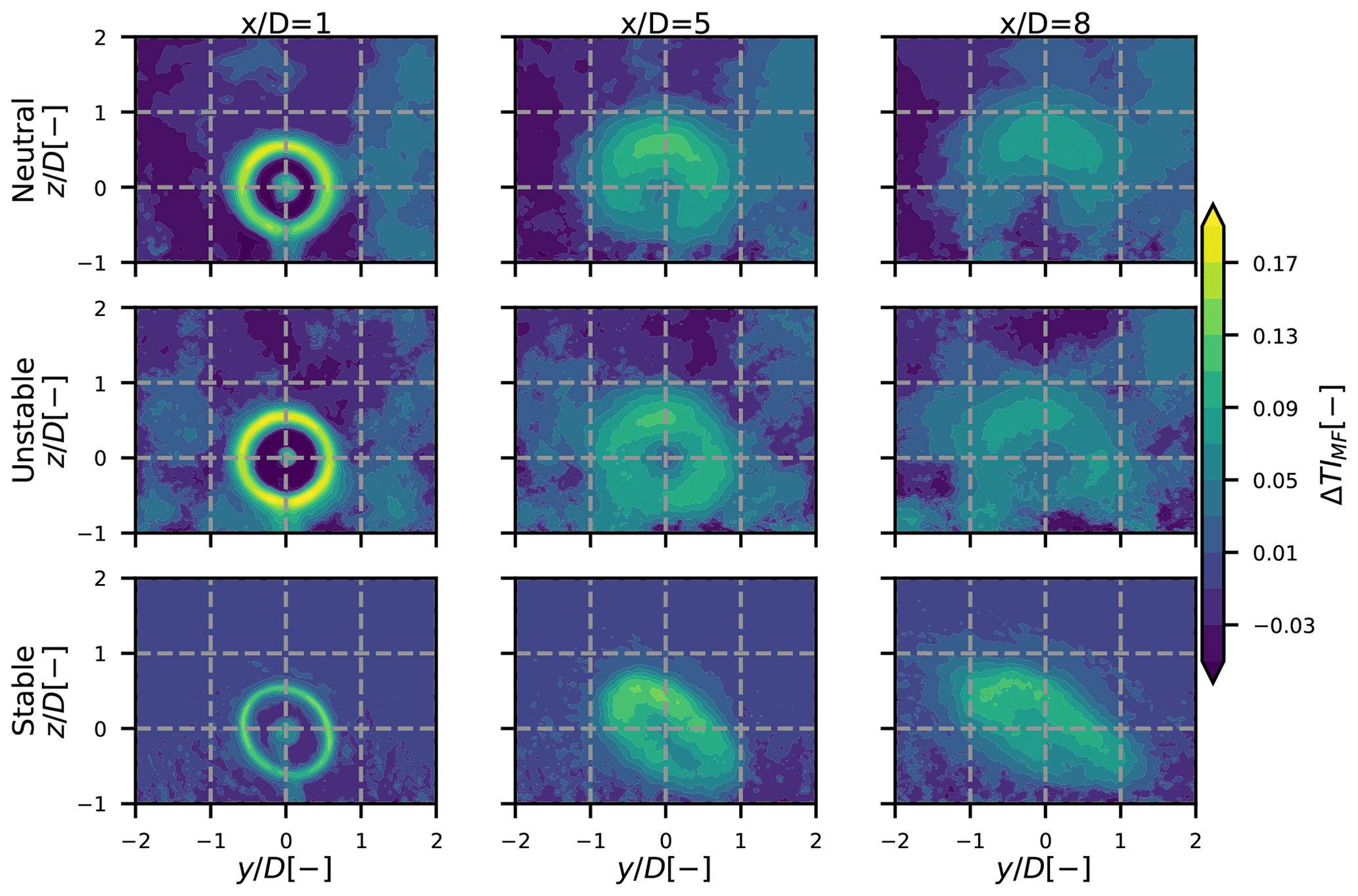
Figure 122D map of the added turbulence in the MFOR, normalized by the velocity at hub height.
Despite strongly different values of Δ(IV) among the different cases, Fig. 12 shows that the atmospheric stability mostly affects meandering and not the field in the MFOR. Indeed, the magnitude of the normalized added TI in the vicinity of the turbine (at ) is about 19 % in the neutral and unstable case, and the slightly lower value in the stable case (about 15 %) is attributed to smaller integral length scales upstream the turbine. These discrepancies are small compared to those observed in the FFOR, where the added TI reaches about 22 %, 27 % and 16 % for the neutral, unstable and stable cases (Jézéquel et al., 2022). The skewed shape of the stable case is attributed to the veer that appears in such ABL, but is negligible in neutral and unstable ABL. As the wake travels downstream, the asymmetry increases, in particular for the neutral and stable cases, but the magnitudes of ΔTI are still similar among the different cases despite different values of atmospheric stability, shear and hub height velocity. The asymmetry is attributed to the ambient shear, which increases with atmospheric stability. Negative values of ΔkMF are observed in the near wake between the wake centre and the edge in the neutral and unstable cases and also in the bottom of the far wake in the neutral case. This indicates a transfer of energy from such regions to the high turbulence region, i.e. the edge and the top of the wake. Overall, this figure shows that the different values of Δ(IV) among the cases mainly come from the meandering operation and only slightly from the MFOR turbulence itself.
The value of the cross terms (V), (VI) and (VII) is zero either if there is no meandering (i.e. ) or if there is no turbulence in the MFOR (). Even though the latter can be assumed in some models, none of these conditions is fulfilled in real cases. It has been chosen to regroup the two terms into one single covariance term (V), since those two terms were very large (in absolute value), compensating each other, and thus hard to interpret. Mathematically, this covariance term quantifies how the mean and varying parts of UMF evolve together once displaced by the meandering operation . In the near wake, the non-zero values are distributed at the tip of the blades and then gradually expand in the whole wake. Negative and positive values are symmetrically distributed (along the horizontal and vertical axis for the neutral and unstable cases respectively). From these results, no physical interpretation nor a relation between the values of Ux or kx in the wake with term (V) could be found yet. Modelling the covariance term has thus not been achieved in the companion paper, but the authors are confident that it is an important step toward improvements of wake models based on the meandering. If more data were available, one could perform an ensemble average and hopefully find a shape easier to interpret for this term.
Term (VI) can be viewed as the varying part of turbulence: before being moved by the meandering and averaged, this term is the varying part of the square of the deviation from the mean (in opposition to kx,MF which is the mean part of the square of the deviation from the mean). In the near wake, positive values are present at the tip of the blades in the neutral and unstable cases, but also outside of the wake. It then gradually expands in the whole wake and seems randomly distributed in the wake region with negative and positive values. From Figs. 8–10, it seems that except for systematic negative values near the ground ( D), this term mainly reproduces the spatial non-homogeneity of the wake and is thus not vital to be represented in an analytical model.
Term (VII) is always negative from its mathematical formulation: similarly to the viscous dissipation in the Navier–Stokes equations, it is a sink of energy. It has negligible values in all the stability cases. This last result should be taken with care: if the analogy with the viscous dissipation holds for this term, it means that it concerns small-scale eddies, i.e. variations of the wind velocity at high frequency. Yet, as explained in Sect. 3, only the variations of time scales larger than 1 s are captured with the post-processing used in this work because of memory limitations. With a sampling frequency higher than 1 Hz, this term may have higher values.
It is important to note that all these results are sensitive to the wake tracking method: despite that the method used here being among the most reliable available in the literature, there are always frames where the tracking failed, plus the limitations described in Sect. 3.5. For instance, the turbulence field in the MFOR (see Fig. 12) is noisier and noisier because the wake travels downstream and in particular in the unstable case, which can be interpreted as a consequence of the tracking algorithm being less and less reliable. This remark can be extended to all the terms of the turbulence equation presented in Figs. 8–10. Moreover, the values and shapes of the different terms (in particular the cross terms) might also change depending on the turbulence field, i.e. the eddies of the ABL, even for similar mean atmospheric conditions.
In models predicting wake meandering such as the DWM, it is assumed that the turbulence in the wake can be separated into two parts: the turbulence generated by the rotor and the turbulence generated by meandering. In this work, the turbulence in the FFOR has been developed as a function of the two terms aforementioned, and it appears that three cross terms are missing, thus implicitly neglected in DWM-type models. A similar conclusion is drawn for the velocity, with one missing term.
To quantify the importance of each of these terms and estimate the error induced by the assumptions of such models, LESs with an actuator line are performed to model the wake of an isolated wind turbine inside an ABL. The modelled turbine is the modified Vestas V27 used in the SWiFT campaign of measurements, and three cases of atmospheric stability are investigated: near-neutral, unstable and strongly stable. The instantaneous wake centre is detected at different planes downstream of the turbine (from 1 to 8 D) to compute the velocity field in the MFOR. The main conclusions are the following:
-
Neglecting the cross term of the mean velocity equation leads to small differences in the computation of the mean velocity profile in the FFOR. For the neutral case, the corresponding error leads to a less than 2 % overestimation of the available power in the wake of the wind turbine for a turbine located further than 3 D behind the wake emitting rotor.
-
Neglecting cross terms in the computation of turbulence in the FFOR leads to vertical profiles where the imbalance between the turbulence at the bottom tip and the top tip is underestimated. Adding the three missing cross term allows us to correct this error and reduce the overall RMSE.
-
In the unstable case, the meandering term is dominating the total streamwise turbulence whereas in the stable case, it is the turbulence added by the rotor which is dominant. In the neutral case, these two terms are of similar magnitude and overall larger than the cross terms. These cross terms, especially the so-called covariance term, however show local values sufficiently strong to significantly correct the maximum axial turbulence in the wake.
The statistical convergence of the data has been assessed and showed that increasing the sampling frequency would most likely improve the reliability of the stable case but would have little effect on the two other cases. On the other hand, increasing the simulation time would probably change the unstable results but has a low impact on the other cases. The uncertainty is the highest on the cross terms of the turbulence breakdown equation, but the pure terms are subject to only small uncertainty. For a better interpretation of these terms, it may be important to perform ensemble simulations to get more reliable fields.
It must be noted that these conclusions are drawn on the results of three particular cases of atmospheric stability and one model of turbine that can be regarded as rather small compared to modern rotors. The orders of magnitude given in this work should not be considered universal but are a good indication that for an accurate version of DWM-type models, the cross terms (or at least the covariance term) must be taken into account. In the companion paper, an analytical model for the dominant terms is developed on the neutral and unstable cases presented herein.
In this Appendix, an analysis of the statistical convergence of the three simulations is proposed to give a glimpse to the reader of the uncertainty of the presented data. Indeed, the quality of our data is limited in two ways:
-
First, a sampling frequency of 1 Hz has been set for the three simulations. This value has been chosen accordingly to the SWiFT benchmark (Doubrawa et al., 2020), from which the present simulations are inspired. However, one can argue that it does not sufficiently capture the small-scale variations of the signal.
-
Moreover, a length of 80 min was initially the target for the three simulations. However, the unstable simulation is computationally expensive, and the stable simulation diverges to unrealistic results if it runs for too long due to the strong negative heat flux. Consequently, the segment length was reduced to 40 and 10 min for the unstable and stable cases respectively. Even for the 80 min though, it is not sure a priori that the simulation has run for long enough to have statistically converged results.
These two points have been investigated independently with two different methods in this Appendix. They are used to quantify the uncertainty on every term of Eq. (15) and on kx,MF, for the three simulation cases. Figures A1–A4 thus allow us to respectively estimate the uncertainty of the quantities plotted in Figs. 8, 9, 10 and 12 for the estimation of the corresponding uncertainty. Obviously, this statistical convergence study can be expanded to other quantities, but the aforementioned are considered to be the core of the present work.
A1 Sampling frequency
In the most refined domain, the Meso-NH code runs at a time step close to the millisecond (see Table 1). Thus, estimating the statistics (mean, variance) of the wind velocity from a signal sampled at a frequency of 1 Hz is equivalent to estimating statistics on a reduced population. In our case, the sample time is much greater than 1 s (at least 600 s in the stable case), but much lower than the actual time step of the signal (which is about 1 ms, depending on the Meso-NH time-step). In such a case, the law of large numbers indicates that the mean computed on the reduced size population is a random variable which follows a normal law. The 95 % confidence interval of the mean of a variable X computed from a population of reduced size can thus be computed as
where σX is the standard deviation of the variable X and n is the sample size. The turbulence and every term of Eq. (15) can be written as the mean of a given variable, except for term (VII). Consequently, Eq. (A1) is applied on the time series corresponding to each of these terms, before the time averaging is applied. For instance, for term (III), it gives
For term (VII), it is assumed that the confidence interval is equal to the square of the confidence interval of term (II). This may be a strong approximation, but this term is anyway found to be negligible, and thus plays only a small role in the total turbulence budget.
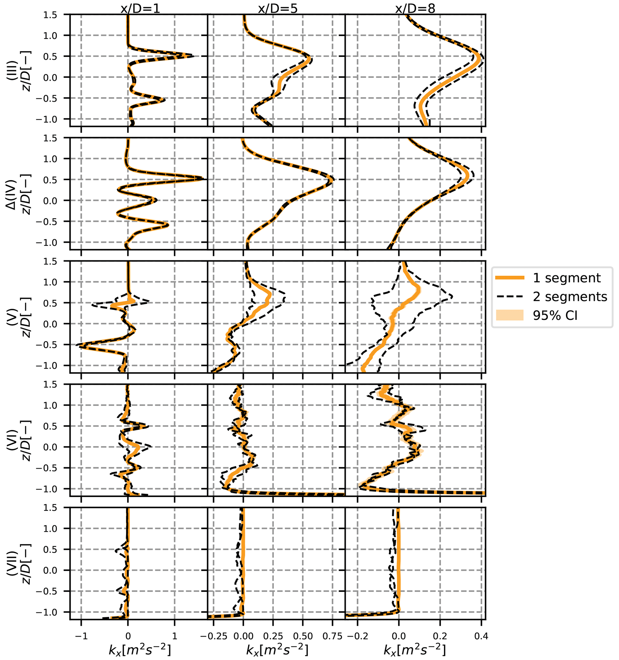
Figure A1Vertical profiles at y=0 of the different terms of the turbulence breakdown equation, for the neutral case. The 95 % confidence area is plotted with a shaded area and the results with two sub-segments in dotted black lines. The different rows stand for the different terms, and each column is a different position: 1, 5 and 8 D downstream.
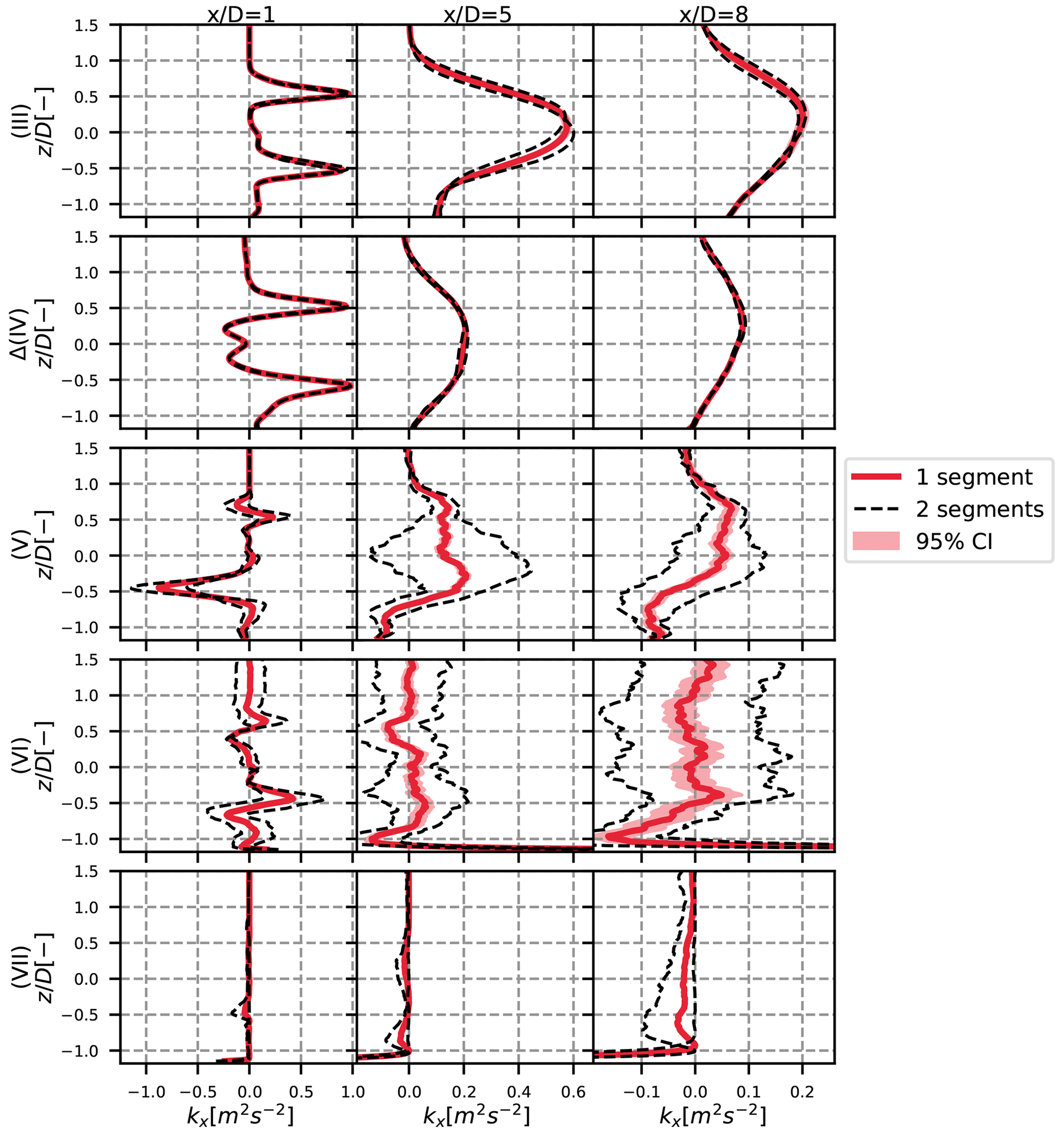
Figure A2Vertical profiles at y=0 of the different terms of the turbulence breakdown equation, for the unstable case. The 95 % confidence area is plotted with a shaded area and the results with two sub-segments in dotted black lines. The different rows stand for the different terms, and each column is a different position: 1, 5 and 8 D downstream.
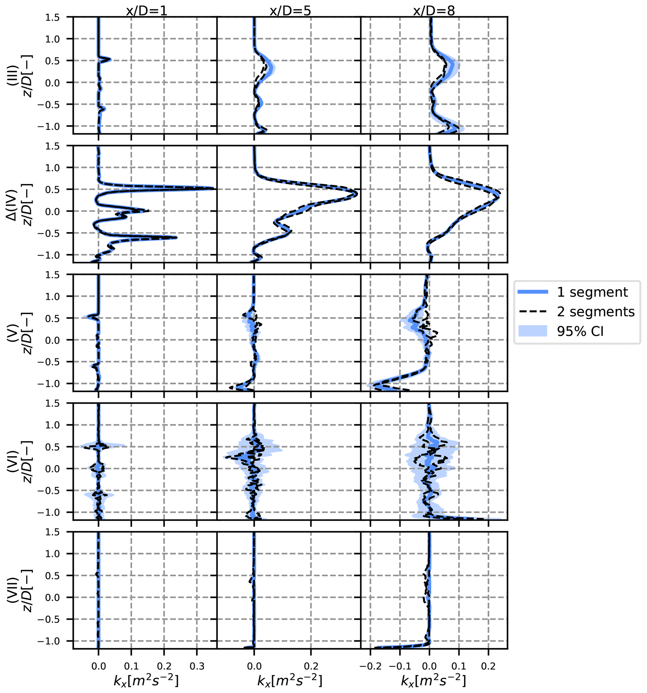
Figure A3Vertical profiles at y=0 of the different terms of the turbulence breakdown equation, for the stable case. The 95 % confidence area is plotted with a shaded area and the results with two sub-segments in dotted black lines. The different rows stand for the different terms, and each column is a different position: 1, 5 and 8 D downstream.
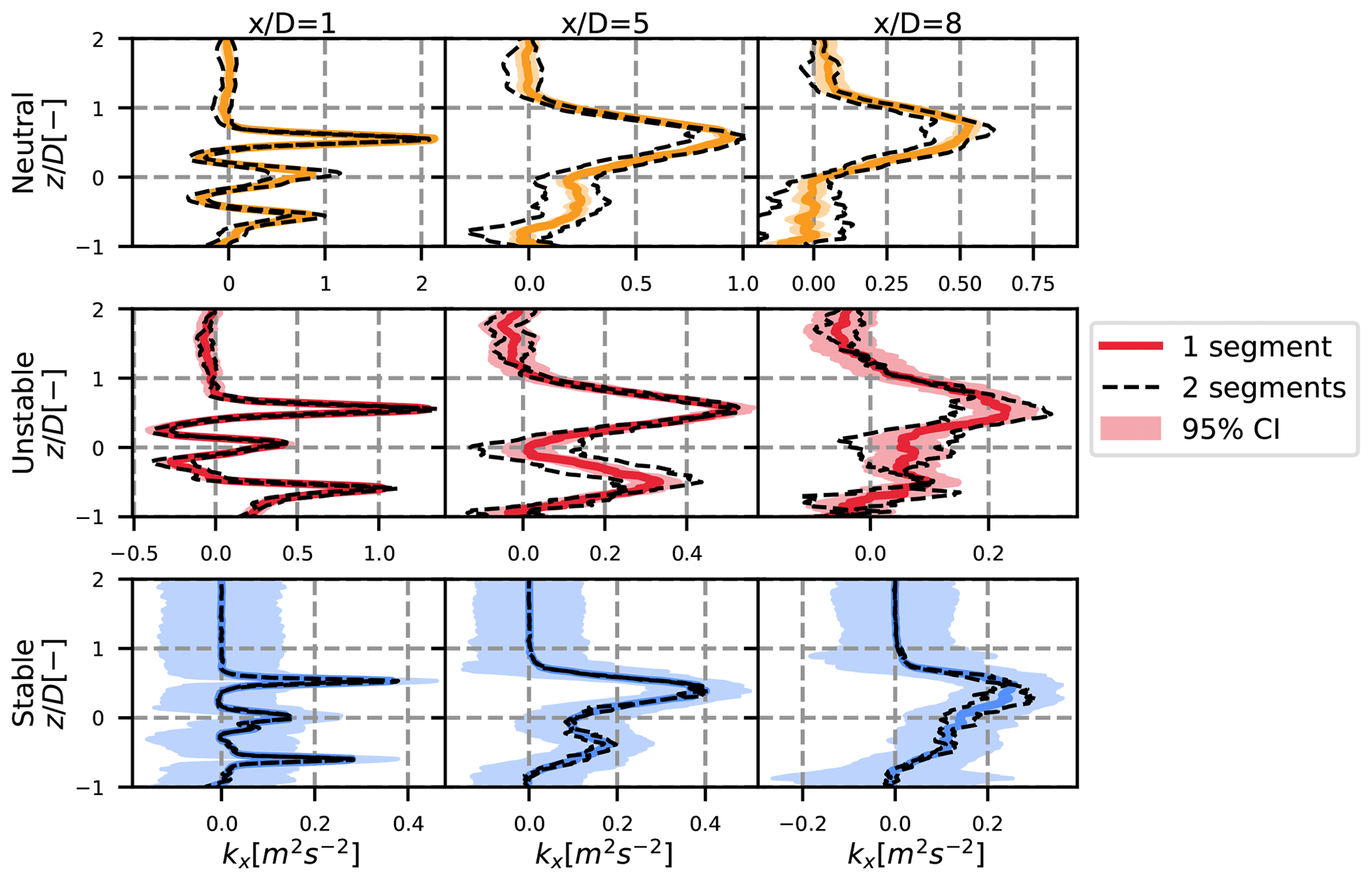
Figure A4Vertical profiles at y=0 of the streamwise turbulence in the MFOR. The 95 % confidence area is plotted with a shaded area and the results with two sub-segments in dotted black lines. The different rows stand for the different cases, and each column is a different position: 1, 5 and 8 D downstream.
The confidence interval is plotted in the shaded area in Figs. A1–A4. It appears that there is a strong confidence in our results for the pure terms – terms (III) and (IV) – of the turbulence breakdown equation (Figs. A1–A3). The cross terms, in particular term (VII) in the stable case, seem to be less reliable, but the results can still be considered satisfying. However, the confidence interval is more important for the MFOR turbulence, in particular for the stable case (Fig. A4).
This confidence interval quantifies the uncertainty towards the small-scale turbulence. It is thus not surprising that it gets higher values in the stable case (where turbulence is mostly of small scale) and in particular for the turbulence in the MFOR and for term (VI), which is attributed to the spatial non-homogeneity, and thus to the small-scale variation. A higher sampling frequency for the stable case would seemingly improve the reliability of the simulation, but for the two other cases, the sampling at 1 Hz seems suitable.
A2 Length of the simulations
The length of the simulations (80, 40 and 10 min for the neutral, unstable and stable cases) has been arbitrarily chosen depending on numerical constraints. Even though some works in the literature are based on 10 min long simulations, it should be ensured that this choice is sufficient to take into account all the large-scale variations of the ABL.
To do so, the velocity time series are separated into two equal sub-segments (thus of length 40, 20 and 5 min for the neutral, unstable and stable cases). The whole post-process is reproduced on these sub-segments, and the resulting profiles are plotted in dashed black lines in Figs. A1–A4. One can argue that if the sub-segments are similar to the full simulation, increasing further the computational time would likely have no effect, whereas if significant differences are observed, the simulation is probably not well converged. Note that it is normal if the mean of the two sub-segments (dashed black line) is not exactly equal to the full segment (continuous coloured line), because statistics of higher order than averages are at stake. For instance, the total variance is always larger than the mean of the sub-segments variables.
This concept of convergence should however be taken with care here, because the ABL is in permanent evolution due to the constant heat flux at the ground that changes progressively its characteristics. This is particularly true for the unstable case where the mean wind direction is not equal among the two sub-segments and where the atmospheric conditions will likely never reach a quasi-steady state.
Conversely to the sampling frequency, this method measures the uncertainty of the large-scale turbulence. It is thus not surprising to see that the uncertainty is higher in the unstable case (Fig. A2). Again, the uncertainty is higher on the cross terms, and in particular on term (VI). For the turbulence in the MFOR, the uncertainty due to the length of the simulations is limited, which is consistent with the fact that there are supposedly only small-scale variations in this frame and, thus, increasing the segment length would likely have no effect.
As a conclusion, a higher sampling frequency could give more reliable results in the stable case, and a longer simulation time may have been needed for the unstable case. This is particularly true for term (VI) which has the largest level of uncertainty. Nevertheless, the uncertainty on the other terms and the streamwise turbulence in the MFOR seem sufficiently low to maintain the conclusions drawn at the core of this article.
The code Meso-NH is open-source and can be downloaded on the dedicated website (http://mesonh.aero.obs-mip.fr/mesonh54/, Rodier, 2023). The authors can provide the source code of the modified version 5-4-3 that was used in this work. The results of the LES simulations can also be directly provided.
EJ developed the equations and performed the simulations with VM. All the authors worked on the interpretation of the results. The manuscript has been written by EJ with the feedback of FB and VM. The data used for the plot presented here and in Part 2 are available under this online deposit: https://doi.org/10.5281/zenodo.6562720 (Jézéquel, 2022).
The contact author has declared that none of the authors has any competing interests.
Publisher's note: Copernicus Publications remains neutral with regard to jurisdictional claims in published maps and institutional affiliations.
This paper was edited by Raúl Bayoán Cal and reviewed by two anonymous referees.
Abkar, M. and Porté-Agel, F.: Influence of atmospheric stability on wind-turbine wakes: A large-eddy simulation study, Phys. Fluids, 27, 035104, https://doi.org/10.1063/1.4913695, 2015. a
Ainslie, J. F.: Calculating the flowfield in the wake of wind turbines, J. Wind Eng. Indust. Aerodynam., 27, 213–224, https://doi.org/10.1016/0167-6105(88)90037-2, 1988. a
Brugger, P., Markfort, C., and Porté-Agel, F.: Field measurements of wake meandering at a utility-scale wind turbine with nacelle-mounted Doppler lidars, Wind Energ. Sci., 7, 185–199, https://doi.org/10.5194/wes-7-185-2022, 2022. a
Conti, D., Dimitrov, N., Peña, A., and Herges, T.: Probabilistic estimation of the Dynamic Wake Meandering model parameters using SpinnerLidar-derived wake characteristics, Wind Energ. Sci., 6, 1117–1142, https://doi.org/10.5194/wes-6-1117-2021, 2021. a, b, c
Cuxart, J., Bougeault, P., and Redelsperger, J.-L.: A turbulence scheme allowing for mesoscale and large-eddy simulations, Q. J. Roy. Meteorol. Soc., 126, 1–30, https://doi.org/10.1002/qj.49712656202, 2000. a
Deardorff, J. W.: Stratocumulus-capped mixed layers derived from a three-dimensional model, Bound.-Lay. Meteorol., 18, 495–527, https://doi.org/10.1007/bf00119502, 1980. a
Doubrawa, P., Quon, E. W., Martinez-Tossas, L. A., Shaler, K., Debnath, M., Hamilton, N., Herges, T. G., Maniaci, D., Kelley, C. L., Hsieh, A. S., Blaylock, M. L., Laan, P., Andersen, S. J., Krueger, S., Cathelain, M., Schlez, W., Jonkman, J., Branlard, E., Steinfeld, G., Schmidt, S., Blondel, F., Lukassen, L. J., and Moriarty, P.: Multimodel validation of single wakes in neutral and stratified atmospheric conditions, Wind Energy, 23, 2027–2055, https://doi.org/10.1002/we.2543, 2020. a, b, c
Du, B., Ge, M., Zeng, C., Cui, G., and Liu, Y.: Influence of atmospheric stability on wind turbine wakes with a certain hub-height turbulence intensity, Phys. Fluids, 33, 055111, https://doi.org/10.1063/5.0050861, 2021. a
Fuertes, F. C., Markfort, C., and Porté-Agel, F.: Wind Turbine Wake Characterization with Nacelle-Mounted Wind Lidars for Analytical Wake Model Validation, Remote Sens., 10, 668, https://doi.org/10.3390/rs10050668, 2018. a
Ishihara, T. and Qian, G.-W.: A new Gaussian-based analytical wake model for wind turbines considering ambient turbulence intensities and thrust coefficient effects, J. Wind Eng. Indust. Aerodynam., 177, 275–292, https://doi.org/10.1016/j.jweia.2018.04.010, 2018. a
Jézéquel, E.: Figures data from papers “Breakdown of the velocity and turbulence in the wake of a wind turbine”, parts 1 and 2, Zenodo [data set], https://doi.org/10.5281/zenodo.6562720, 2022. a
Jézéquel, E., Cathelain, M., Masson, V., and Blondel, F.: Validation of wind turbine wakes modelled by the Meso-NH LES solver under different cases of stability, J. Phys.: Conf. Ser., 1934, 012003, https://doi.org/10.1088/1742-6596/1934/1/012003, 2021. a, b, c
Jézéquel, E., Blondel, F., and Masson, V.: Analysis of wake properties and meandering under different cases of atmospheric stability: a large eddy simulation study, J. Phys.: Conf. Ser., 2265, 022067, https://doi.org/10.1088/1742-6596/2265/2/022067, 2022. a, b, c
Joulin, P.-A., Mayol, M. L., Masson, V., Blondel, F., Rodier, Q., Cathelain, M., and Lac, C.: The Actuator Line Method in the Meteorological LES Model Meso-NH to Analyze the Horns Rev 1 Wind Farm Photo Case, Subduct. Zone Geodynam., 7, 350, https://doi.org/10.3389/feart.2019.00350, 2020. a, b
Keck, R.-E., Maré, M. D., Churchfield, M. J., Lee, S., Larsen, G., and Madsen, H. A.: On atmospheric stability in the dynamic wake meandering model, Wind Energy, 17, 1689–1710, https://doi.org/10.1002/we.1662, 2013a. a
Keck, R.-E., Maré, M. D., Churchfield, M. J., Lee, S., Larsen, G., and Madsen, H. A.: Two improvements to the dynamic wake meandering model: including the effects of atmospheric shear on wake turbulence and incorporating turbulence build-up in a row of wind turbines, Wind Energy, 18, 111–132, https://doi.org/10.1002/we.1686, 2013b. a, b, c
Lac, C., Chaboureau, J.-P., Masson, V., Pinty, J.-P., Tulet, P., Escobar, J., Leriche, M., Barthe, C., Aouizerats, B., Augros, C., Aumond, P., Auguste, F., Bechtold, P., Berthet, S., Bielli, S., Bosseur, F., Caumont, O., Cohard, J.-M., Colin, J., Couvreux, F., Cuxart, J., Delautier, G., Dauhut, T., Ducrocq, V., Filippi, J.-B., Gazen, D., Geoffroy, O., Gheusi, F., Honnert, R., Lafore, J.-P., Brossier, C. L., Libois, Q., Lunet, T., Mari, C., Maric, T., Mascart, P., Mogé, M., Molinié, G., Nuissier, O., Pantillon, F., Peyrillé, P., Pergaud, J., Perraud, E., Pianezze, J., Redelsperger, J.-L., Ricard, D., Richard, E., Riette, S., Rodier, Q., Schoetter, R., Seyfried, L., Stein, J., Suhre, K., Taufour, M., Thouron, O., Turner, S., Verrelle, A., Vié, B., Visentin, F., Vionnet, V., and Wautelet, P.: Overview of the Meso-NH model version 5.4 and its applications, Geosci. Model Dev., 11, 1929–1969, https://doi.org/10.5194/gmd-11-1929-2018, 2018. a, b, c
Lafore, J. P., Stein, J., Asencio, N., Bougeault, P., Ducrocq, V., Duron, J., Fischer, C., Héreil, P., Mascart, P., Masson, V., Pinty, J. P., Redelsperger, J. L., Richard, E., and de Arellano, J. V.-G.: The Meso-NH Atmospheric Simulation System. Part I: adiabatic formulation and control simulations, Ann. Geophys., 16, 90–109, https://doi.org/10.1007/s00585-997-0090-6, 1998. a
Larsen, G., Pedersen, A., Hansen, K., Larsen, T., Courtney, M., and Sjöholm, M.: Full-scale 3D remote sensing of wake turbulence – a taster, J. Phys.: Conf. Ser., 1256, 012001, https://doi.org/10.1088/1742-6596/1256/1/012001, 2019. a
Larsen, G. C., Madsen, H. A., Thomsen, K., and Larsen, T. J.: Wake meandering: a pragmatic approach, Wind Energy, 11, 377–395, https://doi.org/10.1002/we.267, 2008. a, b
Madsen, H. A., Larsen, G. C., Larsen, T. J., Troldborg, N., and Mikkelsen, R.: Calibration and Validation of the Dynamic Wake Meandering Model for Implementation in an Aeroelastic Code, J. Sol. Energ. Eng., 132, 041014, https://doi.org/10.1115/1.4002555, 2010. a
Ning, X. and Wan, D.: LES Study of Wake Meandering in Different Atmospheric Stabilities and Its Effects on Wind Turbine Aerodynamics, Sustainability, 11, 6939, https://doi.org/10.3390/su11246939, 2019. a
Quon, E. W., Doubrawa, P., and Debnath, M.: Comparison of Rotor Wake Identification and Characterization Methods for the Analysis of Wake Dynamics and Evolution, J. Phys.: Conf. Ser., 1452, 012070, https://doi.org/10.1088/1742-6596/1452/1/012070, 2020. a, b
Rodier, Q.: Meso-NH version 4-3, http://mesonh.aero.obs-mip.fr/mesonh54/, last access: 23 January 2023. a
Sørensen, J. N. and Shen, W. Z.: Numerical Modeling of Wind Turbine Wakes, J. Fluids Eng., 124, 393–399, https://doi.org/10.1115/1.1471361, 2002. a
Stein, J., Richard, E., Lafore, J. P., Pinty, J. P., Asencio, N., and Cosma, S.: High-Resolution Non-Hydrostatic Simulations of Flash-Flood Episodes with Grid-Nesting and Ice-Phase Parameterization, Meteorol. Atmos. Phys., 72, 203–221, https://doi.org/10.1007/s007030050016, 2000. a
Stevens, R. J., Martínez-Tossas, L. A., and Meneveau, C.: Comparison of wind farm large eddy simulations using actuator disk and actuator line models with wind tunnel experiments, Renew. Energy, 116, 470–478, https://doi.org/10.1016/j.renene.2017.08.072, 2018. a
Troldborg, N.: Actuator Line Modeling of Wind Turbine Wakes, PhD Thesis, https://backend.orbit.dtu.dk/ws/portalfiles/portal/5289074/Thesis.pdf (last access: 23 January 2023), 2009. a
- Abstract
- Introduction
- Analytical development
- Methodology
- Error induced by neglecting the cross terms
- Analysis and interpretation of the turbulence breakdown
- Conclusions and perspectives
- Appendix A: Statistical convergence of the results
- Code and data availability
- Author contributions
- Competing interests
- Disclaimer
- Review statement
- References