Spatio-temporal graph neural networks for power prediction in offshore wind farms using SCADA data

This paper introduces a novel model for predicting wind turbine power output in a wind farm at a high temporal resolution of 30 s. The wind farm is represented as a graph, with graph neural networks (GNNs) used to aggregate selected input features from neighboring turbines. A temporal component is introduced by feeding a time series of input features into the graph, processed through a long short-term memory (LSTM) network before being passed to the GNN. Our model is integrated into a normal behavior model (NBM) framework for analyzing power loss events in wind farms. The results show that both the spatial and the spatio-temporal GNN models outperform traditional data-driven power curve methods, achieving reductions in the mean absolute error (MAE) of approximately 22.6 % and 30.3 %, respectively, and in the mean absolute percentage error (MAPE) of around 20.7 % and 30.5 %, respectively. Notably, the spatio-temporal GNN demonstrates superior performance, attributed to its ability to effectively capture both spatial and temporal dynamics. Additionally, the model achieves remarkable agreement with SCADA-derived energy ratios across the full range of wind directions, with a weighted average error of 0.0373, an improvement of approximately 57.4 % compared to the power curve binning method. This advantage is especially pronounced under waked conditions, where traditional methods such as the power curve and multilayer perceptron (MLP) models exhibit significantly higher error rates. Beyond power prediction, we illustrate the model's effectiveness in detecting and analyzing instances of reduced performance and its ability to identify various types of abnormal events beyond what is recorded in standard status logs. Compared to the power curve method, the spatio-temporal GNN reduces the rate of undetected power loss events from 12.6 % to just 0.02 %, demonstrating a substantial improvement in capturing abnormal events.

1 Introduction

Wind energy plays a vital role in addressing the escalating global energy demand while aligning with sustainability goals to combat climate change. As countries worldwide strive to reduce greenhouse gas emissions and transition toward renewable energy sources, wind energy emerges as a clean and abundant resource capable of meeting a significant portion of our energy needs (Yousefi et al., 2019). Offshore wind farms offer promising opportunities to harness stronger and more consistent wind speeds compared to onshore locations, thereby contributing to a more resilient and sustainable energy infrastructure (International Energy Agency, 2023). As technology advances and costs continue to decline, offshore wind projects are becoming more economically viable and attractive investments for governments, developers, and energy consumers alike (European Commission, 2023).

The accurate estimation of potential power allows wind farm operators to optimize the operation of individual turbines and the entire wind farm. By understanding the potential power each turbine could generate under different wind conditions, operators can make informed decisions about operation settings and maintenance schedules to maximize production while minimizing costs. As wind conditions and turbine performance can fluctuate significantly, developing precise power prediction models becomes essential to navigating these complexities.

Building on this need for accurate power forecasts, it is equally important to utilize these predictions to identify power loss events – instances of reduced performance where the generated power falls below the potential output – in the wind farm. By comparing predicted energy output with actual performance, we can detect potential inefficiencies and operational issues.

In this context, this research addresses two key questions:

1. Can we leverage temporal trends in wind flow, turbine positioning, and integrated measurements from different turbines in the wind farm to improve power prediction accuracy?

2. Can we detect power loss events by comparing precise power predictions with actual turbine performance?

Potential power prediction methods can be integrated into a broader performance monitoring framework through the implementation of a normal behavior model (NBM). The essence of NBM lies in training models to recognize normal behavior, enabling the identification of abnormal observations based on low model support. For instance, in the context of a regression-based NBM, training on a dataset representing purely normal behavior enables the detection of abnormalities by identifying deviations from an expected residual of zero when presented with new test set observations.

Additionally, quantifying losses during power loss events enables stakeholders to assess the economic impact of turbine downtime or grid curtailments. High levels of curtailment can lead to increased wear and tear on turbines, a reduced operational lifespan, and potential reliability issues (Robbelein et al., 2023). With curtailment strategies evolving to be more dynamic, the need to refine these strategies increases. By quantifying the magnitude and frequency of power losses during curtailments, operators can identify patterns and evaluate the economic impact of curtailments. These data enable operators to implement strategies to reduce curtailment frequency or duration and make informed decisions about investments in grid upgrades or energy storage solutions that could mitigate future losses.

Finally, the development of state-of-the-art wind farm control methods typically relies on models that capture the wake effect between wind turbines (Verstraeten et al., 2021). Wake effects are highly nonlinear and difficult to capture and are traditionally modeled using physics-based wake models that can be calibrated using real-world data (van Binsbergen et al., 2024a, b, c). In this work, we propose a model to predict the potential power of wind turbines operating in wakes, specifically designed for wind farm control applications. The model utilizes integrated measurements from the supervisory control and data acquisition (SCADA) system of multiple turbines at a high temporal resolution of 30 s.

The remainder of this paper is structured as follows: in Sect. 2, we position our research within the context of existing literature. Section 3 details our approach, including the data-processing pipeline, the GNN framework, and the training and hyperparameter tuning process of our models. Section 4 presents a comprehensive analysis of the model's performance, including its predictive accuracy and ability to detect abnormal events, compared to baseline methods. In Sect. 5, the most important results are further discussed, and finally, in Sect. 6, we summarize the key findings of our study and outline potential directions for further research.

2 Related work

An example of an NBM for performance analysis, based on an artificial neural network trained on an abnormality-filtered SCADA dataset for power prediction, is shown by Lyons and Gocmen (2021). The authors demonstrate the effectiveness of the developed NBM for power performance analysis by qualitatively discussing instances of over- and underperformance identified by the model. However, the NBM seemed to struggle to model power production at higher wind speeds and expressed a tendency to underestimate the wake effect at play in the farm. In another study by Bilendo et al. (2022), a different NBM is introduced for condition monitoring of wind turbines, leveraging a heterogeneous stacked regressor (HET-SR) algorithm. This algorithm learns from optimal power curve data to serve as a predictive model within the NBM framework. While a qualitative analysis of a variety of faults that can be detected by the model is shown, employing more advanced prediction models that account for additional variables beyond wind speed could offer opportunities for a more comprehensive performance analysis beyond general fault detection.

Traditionally, the manufacturer's power curve, which describes the theoretical behavior of a wind turbine in constant and low-turbulence wind conditions, is used to predict the expected power output at different wind speeds. However, this method fails to account for the specific atmospheric conditions in a particular wind farm. Therefore, most wind farm operators use the method of binning (International Electrotechnical Commission (IEC), 2017) to estimate the power curve based on measurement data from their own wind turbines. With this method, the range of measured wind speeds is partitioned into separate bins of 0.5 m s⁻¹, and the power response is calculated by averaging the power data falling in each bin. While this method is easy to implement and can capture the primary nonlinear relationship between wind speed and power output, it does not account for inter-turbine interactions and varying environmental conditions such as turbulence intensity.

These limitations are particularly important in large wind farms, where wake losses and other complex dynamics become more prevalent. Modeling these wake losses and the flow patterns within the farm has been an active area of research, and various approaches have been devised to predict expected power in wake-affected wind farms. These methods can be categorized as either physics based or data driven (or a combination of the two).

Physics-based models aim to model the wind and wake flows within the wind farm based on prior knowledge of the physical behavior of the system. These models range from low to high fidelity, depending on the amount of detail they capture. Low-fidelity models are relatively fast but neglect lots of details in modeling the wind flow. An example is the FLOw Redirection and Induction in Steady State (FLORIS) model developed at NREL, a control-focused wind farm simulation software incorporating steady-state engineering wake models into a Python framework (NREL, 2024). On the other hand, high-fidelity models describe the flow in detail based on the 3D Navier–Stokes equations and use large-eddy simulations (LES) to accurately resolve the turbulent flow structures, but they are limited by their high computational cost. Examples of high-fidelity models are SOWFA (Simulator for Offshore Wind Farm Applications; NREL, 2012) and PALM (Raasch and Schröter, 2001).

Data-driven models construct relationships between the inputs and outputs based on statistical or machine learning models, without prior knowledge of the physical behavior of the process. Recent advancements in deep learning and big data resulted in a growing interest in wind farm power prediction using deep learning methods. For instance, Lin and Liu (2020) provided a comprehensive overview of prior studies employing deep learning methods and introduced a predictive model using deep learning in conjunction with high-frequency SCADA data. Similarly, Lyons and Gocmen (2021) delved into power prediction tasks using deep learning, utilizing high-frequency SCADA data and integrating local information from neighboring turbines to enhance predictive accuracy. Moreover, the significance of spatio-temporal factors influencing wind power generation was addressed in Zhang et al. (2021) and Yin et al. (2021), who employed specialized model architectures such as convolutional neural networks (CNNs) and long short-term memory networks (LSTMs) to extract spatial and temporal feature information. Finally, Daenens et al. (2024) developed a turbine-level power prediction model, incorporating high-frequency SCADA data from neighboring turbines into a prediction model for potential power based on a hybrid CNN-LSTM model architecture by organizing the input data into a grid structure based on the wind farm layout.

A different approach to represent the spatial correlations between wind turbines in a wind farm is the use of graphs. Graphs can be used to represent complex data that are not inherently structured in a grid-like manner, allowing for arbitrary connections between nodes through edges. This approach has proven beneficial for wind farms in previous studies. For example, Verstraeten et al. (2021) utilized coordination graphs to develop scalable wind farm control strategies, effectively decomposing large-scale multi-agent optimization problems. In another study, Hammer et al. (2023) represented the wind farm as a graph and employed an extreme gradient boosting model to predict the wake interaction losses between turbine pairs.

Graph neural networks (Scarselli et al., 2009) have emerged as powerful tools for learning on graph-structured data. GNNs leverage the structure of the graph to learn rich node representations by iteratively aggregating information from neighboring nodes. They are particularly well suited for tasks that involve node-level predictions, such as power prediction in wind farms.

For example, Bleeg (2020) introduced GNNs as surrogate models for steady-state Reynolds-averaged Navier–Stokes (RANS) simulations, providing a more computationally efficient alternative to traditional RANS models while maintaining reasonable accuracy. More complex GNNs are explored in the work of Park and Park (2019) and Bentsen et al. (2022), where the former proposed a physics-induced GNN (PGNN) and the latter an attention-based GNN for the power prediction of individual wind turbines in a wind farm. Both these methods use synthetic wind farm data simulated using the FLORIS model.

In a different application, de N Santos et al. (2024) presented a GNN framework for the layout-agnostic modeling of fatigue load effects. Using graph representations derived from PyWake (Pedersen et al., 2023) simulations, with inflow conditions as inputs and geometrical properties encoded on edges, the framework models wind farm dynamics across various layouts and conditions.

Combining the spatial and temporal aspects of wind farm dynamics, Yu et al. (2020) developed the superposition graph neural network, a spatio-temporal model that processes a time series of graphs to predict the power output of the wind turbines in a wind farm. This model was trained on data for four offshore wind farms sampled at 10 min intervals and showcases the capability of GNNs to capture the evolution of wind flow through the farm and its impact on power generation.

3 Methodology

The data-driven methodology proposed in this work leverages high-resolution SCADA data to predict the potential power for each wind turbine in a wind farm. In this section, we describe the key aspects of our modeling framework, and we show the design choices that were made to develop a unified framework that can be applied to any wind farm. The data as well as the preprocessing pipeline are described in detail in Sect. 3.1. In Sect. 3.2, the graph representation of the wind farm is introduced. The different model architectures and characteristics are elaborated on in Sect. 3.3, and finally, the hyperparameter tuning process is explained in Sect. 3.4.

3.1 Data collection and preprocessing

We considered a wind farm in the Dutch–Belgian offshore zone for this study, consisting of more than 40 turbines with >8 MW rated power. Specifically, the signals obtained by the SCADA system were used, covering a 2-year period from 2021 to 2022. The SCADA system records real-time information at a resolution of 1 Hz, collected from sensors and control systems for monitoring and optimizing turbine performance and overall wind farm operations, which is widely used in the offshore wind industry. As most contemporary wind farms have used input signals that are readily available (e.g., through their SCADA system), the model is easily accessible and applicable to other wind farms.

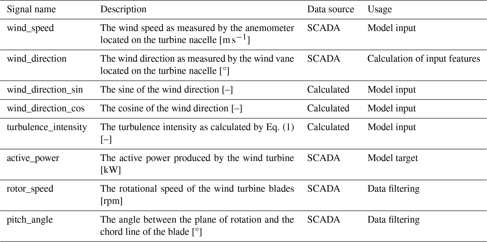
From the SCADA system, the data signals shown in Table 1 were retained and used in our analysis. The input features to the prediction model were wind_speed, wind_direction_sin, wind_direction_cos, and turbulence_intensity. They were chosen because they directly capture the key physical factors influencing wind farm power generation, such as wind resource characteristics, directional influences, and flow variability. Other features were excluded due to data availability limitations, potential redundancy, and a focus on simplifying the model while retaining interpretability and accuracy. Wind speed was taken directly from SCADA data and represents the wind speed at turbine hub height, as measured by the anemometer located on the nacelle. The absolute wind direction, measured by a wind vane mounted on the nacelle, was represented by sine and cosine transformations to account for its circular nature. This approach ensures a smooth representation of wind direction throughout its entire range and prevents issues where a model might incorrectly interpret a large difference between wind directions close to 0 and 360°. Turbulence intensity (TI) refers to the measure of fluctuations in wind speed over time, indicating the variability or instability of the airflow. The TI was calculated using Eq. (1):

$$\begin{array}{}\text{(1)}& \text{TI}={\displaystyle \frac{{\mathit{\sigma }}_{\text{ws}}}{{\mathit{\mu }}_{\text{ws}}}},\end{array}$$

where σ_ws is the standard deviation of wind speed (ws), and μ_ws is the mean wind speed, both computed over a 10 min interval centered around the 1 s data point. In practical terms, this method requires wind speed data from 5 min before and 5 min after each point to compute the turbulence intensity. As a result, any real-time application of this calculation would inherently introduce a 5 min lag, since the full 10 min window is not complete until 5 min after the moment being analyzed. However, in our case, this method is used for historical data analysis rather than real-time predictions, so this lag does not impact the accuracy or usability of our power predictions.

The target of our prediction model is the active_power signal extracted from the SCADA data. Additionally, we included two more SCADA signals: rotor_speed and pitch_angle, which were utilized for filtering normal operational behavior across our training, validation, and test datasets.

Table 1 Overview of data signals and input features.

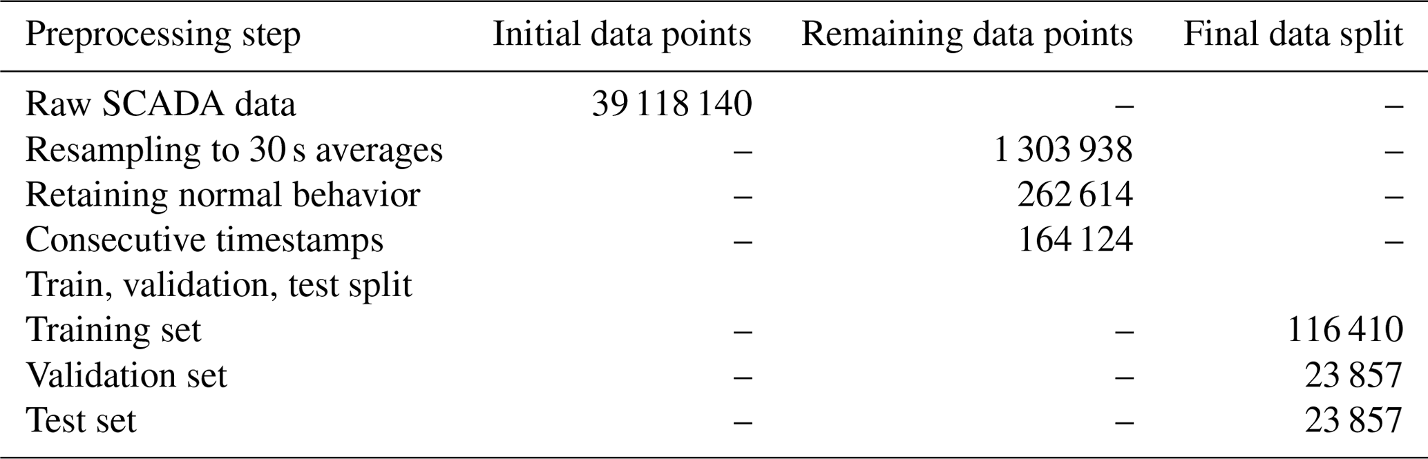
The steps to prepare the raw data for the training, validation, and testing of our prediction model are outlined in Table 2.

First, the raw SCADA data with a sampling frequency of 1 Hz were resampled to 30 s averages as a trade-off between high temporal resolution, acceptable noise levels, and manageable computational costs. This approach smooths out rapid fluctuations while preserving key temporal dynamics. Next, the data were annotated with control conditions for filtering normal behavior. As mentioned previously, to create an NBM capable of accurately detecting abnormal behavior and predicting potential power output under any conditions, the model must be trained exclusively on data that represent normal system behavior.

To achieve this, we used a physics-based filtration method, which relies on the properties of the power curve as per the standards by the International Electrotechnical Commission (IEC) (2017) to annotate steady-state control conditions. Using this approach, we classified the data into different operating regions (i.e., torque control, pitch control), flagged data points falling outside these regions as abnormal, and removed them from the dataset. We removed the entire timestamp across all turbines when any individual turbine exhibited abnormal operation. While this reduces the number of data points available for model training, we found that this approach yields the best results for creating a reliable NBM.

To leverage temporal patterns in the wind flow throughout the wind farm, we incorporated lagged values of the input features into the model. Specifically, a time series of input features between the prediction time t and t−T (with T=5 min) was included. Given the time series nature of the data, it is essential to maintain temporal continuity, so a final filtering step was implemented to ensure that lagged values used by the model are consecutive and free from discontinuities caused by missing data. To ensure continuity in the time series, we required that no timestamps were missing across all turbines for the current and lagged timestamps.

Finally, the resulting dataset was partitioned into distinct subsets for model training, validation, and testing. The first year of data was used as training data to fit the model parameters. The second year of data was split into equal parts as the validation and test set. Validation data are utilized to tune hyperparameters and prevent overfitting, and testing data are used to assess the model's performance on unseen data, ensuring their generalizability.

Table 2 Preprocessing steps and remaining data points.

3.2 Graph representation of the wind farm

With the datasets for training, validation, and testing of the prediction model defined, they were transformed into a format suited to our model. Specifically, the wind farm was represented as a graph, and the selected input features from the SCADA data were converted into graph-structured data.

A graph G is usually defined as a tuple of two sets $G=(V,E)$, where $V=\mathit{\{}{v}_{\mathrm{1}},v_{\mathrm{2}},\mathrm{\dots },v_N\mathit{\}}$ and $E\subseteq V\times V$ are the sets of nodes and edges. To model a wind farm as a graph using this structure, each turbine in the wind farm is represented as a node, and edges connect neighboring turbines. An edge $e_{ij}=(v_i,v_j)\in E$ between nodes v_i and v_j exists if these nodes have line-of-sight visibility, and there are no obstacles (other turbines) blocking the direct view. This visibility check is performed using Algorithm 1.

Algorithm 1 Visibility check.

1:

Input: node1, node2, obstacles, tolerance

2:

Output: true if node1 and node2 are in line of sight, false otherwise

3:

Initialize a flag, visible, to true.

4:

for each obstacle in obstacles do

5:

if obstacle ≠ node1 and obstacle ≠ node2 then

6:

Calculate the distance from node1 to the obstacle, d1.

7:

Calculate the distance from node2 to the obstacle, d2.

8:

Calculate the direct distance between node1 and node2, d_direct.

9:

if $|d\mathrm{1}+d\mathrm{2}-\mathtt{\text{d\_direct}}|<$ tolerance (250 m) then

10:

Set visible to false and break out of the loop.

11:

end if

12:

end if

13:

end for

14:

return  visible, indicating whether node1 and node2 have line-of-sight visibility.

Each node v∈V can be associated with a vector of features x_v∈X, comprising the input features as defined previously. Similarly, a vector of edge attributes can be defined for each edge e∈E, containing a set of geometric features, specifically the length and direction of each edge. Similar to our representation of wind direction, we represented edge direction using its sine and cosine components to account for its circular nature.

3.3 GNN models

At the heart of GNNs is the concept of message passing, a process through which each node in a graph communicates with its neighbors to update its representations (Gilmer et al., 2017). This iterative process can be described in two main steps: message aggregation and node update.

1. Message aggregation. Each node aggregates messages from its neighbors. The nature of this aggregation can vary, but common methods include summation, mean, and max pooling of neighbor features.

2. Node update. After aggregation, each node updates its own feature based on the aggregated message and its previous state. This update is typically performed using a neural network, such as a multilayer perceptron (MLP).

For the task of power prediction, we developed two models: a spatial GNN and a spatio-temporal GNN. The spatial GNN considers the node features only at the current time step, whereas the spatio-temporal GNN also incorporates lagged values of the input features. Both models utilize the GENeralized Graph Convolution (GENConv) model proposed by Li et al. (2020) due to its ability to incorporate edge features into the message-passing process. Its message construction at layer k can be expressed as

$$\begin{array}{rl}& {\mathit{h}}_i^{k+\mathrm{1}}=\text{MLP}({\mathit{h}}_i^k+\text{AGG}(\mathit{\left\{}\text{ReLU}\right({\mathit{h}}_j^k+{\mathit{e}}_{ji})+\mathit{ϵ}:\\ & j\in \mathcal{N}\left(i\right)\mathit{\left\}}\right)),\end{array}$$

where ${\mathit{h}}_i^{\left(k\right)}$ is the representation of node i at the kth layer, e_ji is the feature vector associated with the edge connecting nodes i and j, ϵ is a small positive constant set as 10⁻⁷, and 𝒩(i) denotes the set of neighbors of node i. Finally, AGG represents the aggregation function, with softmax aggregation used in this work.

The spatial GNN model consists of a node and edge feature encoder, followed by a series of message-passing layers, and concludes with a decoder: a dense layer with sigmoid activation to normalize the predictions between 0 and 1. Both of the node and edge encoders are two-layer MLPs. The message-passing layers were implemented using PyTorch Geometric (Fey and Lenssen, 2019) and were constructed according to the GENConv model by Li et al. (2020).

The spatio-temporal GNN model first processes the time series of node features with an LSTM network. Similar to the spatial GNN, this block serves as the node feature encoder; however, in this case, the output of the LSTM network is passed through the GNN model.

An overview of the methodology for power prediction is shown in Fig. 1.

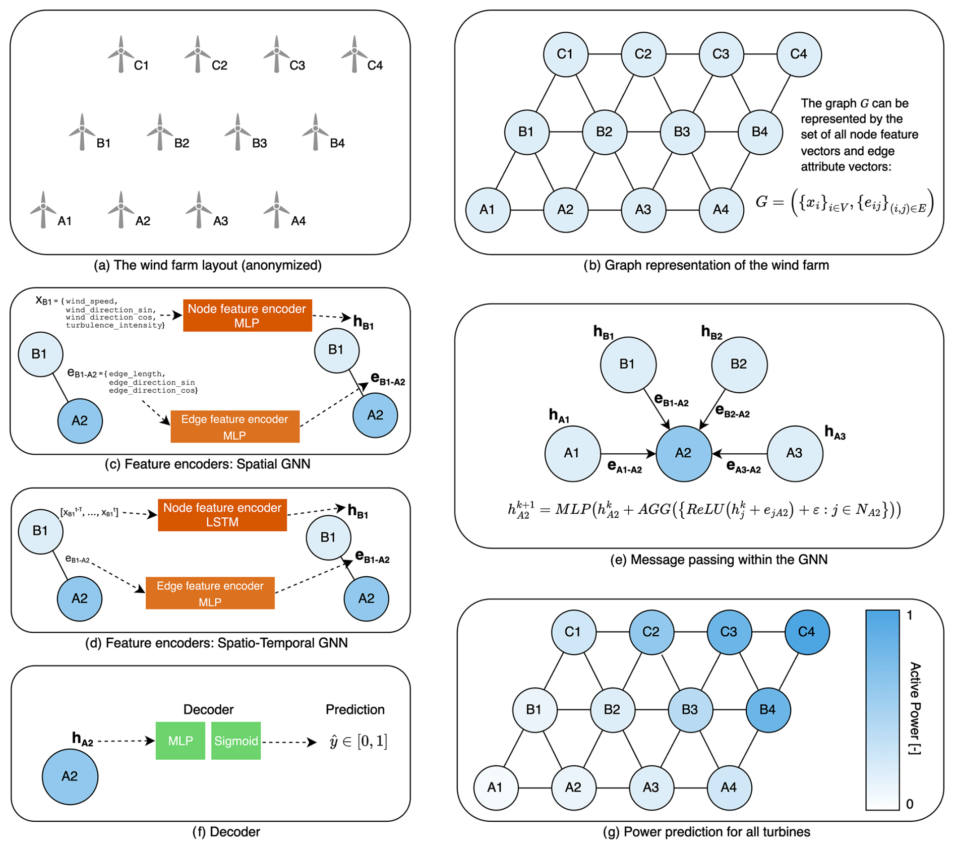
Figure 1 Overview of the proposed methodology for power prediction. The wind farm (a) is represented as a graph (b). The input features are encoded by the encoder blocks. In the spatial GNN, these are MLPs (c). In the spatio-temporal GNN, the time series of node features is encoded using an LSTM network. The edge feature encoder remains the same (d). The GNN learns rich representations for each node in the graph using message passing (e). Each node representation is decoded using an MLP with sigmoid activation to normalize the predictions between 0 and 1 (f). Finally, a power prediction is made for each node in the graph (g).

3.4 Hyperparameter tuning

Hyperparameter tuning is crucial for optimizing a machine learning model's performance and ensuring it generalizes well to unseen data. In this study, we used the hyperparameter optimization framework Optuna (Akiba et al., 2019). Optuna allows users to dynamically construct the parameter search space. It benefits from efficient sampling and pruning algorithms and is easy to set up.

Table 3 lists the hyperparameters that were tuned, along with their proposed ranges, as well as the optimized value for both models. Optuna automatically searched for the optimal hyperparameters by minimizing the objective function, defined as the mean squared error (MSE) between the model’s predictions and the target values. Hyperparameter combinations that resulted in the lowest MSE for the validation dataset were retained and used to build the final models.

Table 3 Hyperparameters, proposed ranges, and optimal values for each model.

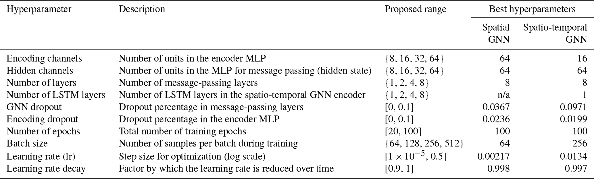
n/a: not applicable

4 Results

In this section, the performance of the different models concerning the specified objectives is discussed. As mentioned in Sect. 3.1, SCADA data of an offshore wind farm comprising over 40 turbines have been used to train and evaluate the spatial and spatio-temporal GNNs described in Sect. 3.3.

4.1 Model performance during normal operation

In Table 4, the mean absolute error (MAE) and the mean absolute percentage error (MAPE) are reported for each model. The models are compared to a power curve model using the power curve binning method (International Electrotechnical Commission (IEC), 2017) as a baseline. Furthermore, we evaluated our models compared to a standard multilayer perceptron (MLP), a commonly used data-driven approach in wind power forecasting. The MLP configuration includes two hidden layers with 64 and 32 units, respectively. The input features for this MLP are wind_speed and turbulence_intensity; wind direction is excluded as it does not directly affect the power output of an individual turbine.

Table 4 Performance metrics. The MAE values have been normalized by dividing them by the turbine's rated power for confidentiality reasons. The lowest errors are highlighted in bold to showcase the model with the best predictive performance on each dataset.

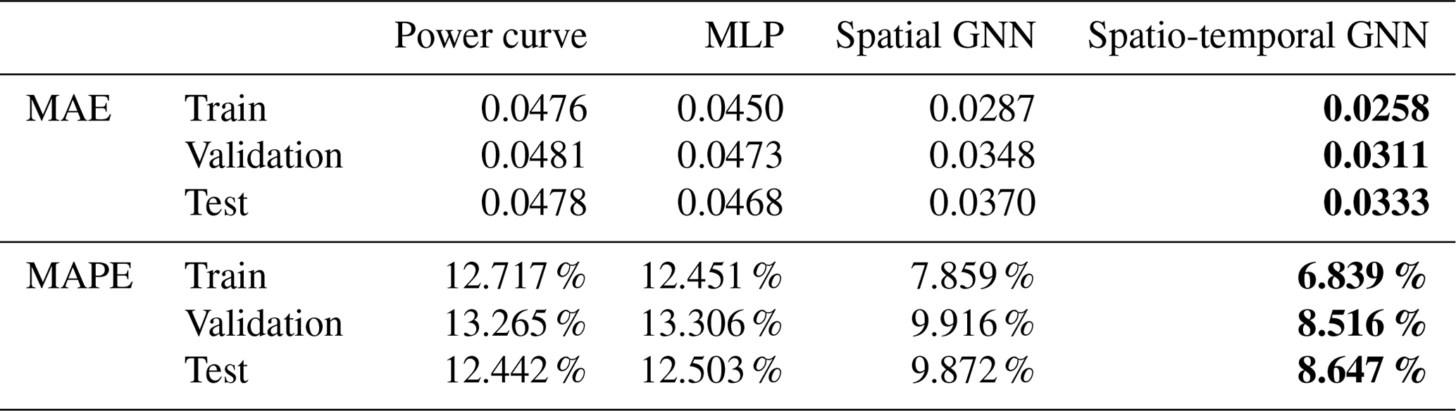
The results indicate that both the spatial GNN and the spatio-temporal GNN models significantly outperform the power curve binning method and the MLP across all metrics and datasets. Specifically, the spatio-temporal GNN model exhibits the best performance, as evidenced by the lowest MAE and MAPE values in the training, validation, and test datasets. Comparatively, while the spatial GNN also outperforms the power curve binning method and the MLP, it falls short of the spatio-temporal GNN. The spatial GNN utilizes input features only at the time of prediction, missing out on the temporal trends that the spatio-temporal GNN can exploit. Therefore, while spatial awareness, integrated measurements, and the ability to model interactions between turbines are crucial, the inclusion of temporal dynamics further enhances predictive accuracy.

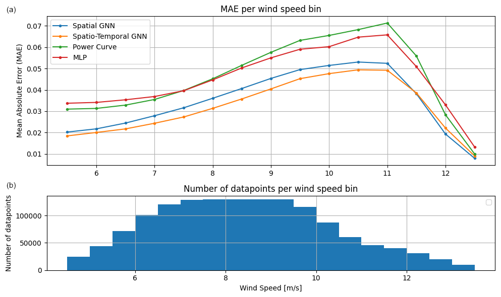
Figure 2 Mean absolute error (MAE) per wind speed bin for the two GNN models, the MLP, and the power curve binning method. Panel (b) shows the number of data points per wind speed bin.

To provide a more granular analysis of our models' predictive performance, Fig. 2 presents the MAEs for different wind speed bins on the test dataset. While the previous analysis highlighted the overall performance of each model across the entire dataset, this plot shows the performance across varying wind speeds.

The analysis shows a slight increase in MAE at higher wind speeds across all models, with a subsequent decrease in errors near the turbine's rated wind speed. This trend aligns with expectations, as higher wind speeds typically result in higher power output and, consequently, larger absolute errors. The observed pattern follows the inherent uncertainties of the power curve, but the models still achieve significantly higher accuracy.

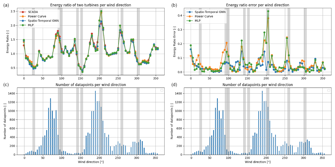
Figure 3 Energy ratio plot (a, c) and energy ratio error plot (b, d) between two turbines for each wind direction as predicted by the spatio-temporal GNN, the power curve binning method, the MLP, and the SCADA data. Panels (c) and (d) show the number of data points in each wind direction bin. Gray-shaded areas indicate waked conditions.

An essential step in model validation involves comparing the model's predictions with historical data, specifically focusing on whether the individual turbine wake losses are accurately predicted. This can be achieved by analyzing the energy ratio between a test turbine and a reference turbine for each wind direction bin (Fleming et al., 2019; Doekemeijer et al., 2022). By examining the predicted energy ratio for each wind direction, we can gain deeper insights into how the model evaluates the impact of wake interactions in the wind farm. In an unbiased model, the energy ratio curves should align closely with those observed in the SCADA data.

The energy ratio R_Energy is defined in Eq. (2) and represents the ratio of the sum of all power measurements between a test turbine and a reference turbine, computed for each wind direction bin. This sum of power measurements over a fixed period is equivalent to the total energy produced during that time. Because the ratio is calculated over the same time period for both the test and the reference turbines, the time factor cancels out. In this equation, $P_{i,\mathit{\theta }}^{\text{Turbine 1}}$ and $P_{i,\mathit{\theta }}^{\text{Turbine 2}}$ are the observed powers of point i in a given wind direction bin for the two test turbines, and N is the number of points in this wind direction bin.

$$\begin{array}{}\text{(2)}& R_{\text{Energy }}\left(\mathit{\theta }\right)={\displaystyle \frac{{\sum }_{i=\mathrm{1}}^N{P}_{i,\mathit{\theta }}^{\text{Turbine 1 }}}{{\sum }_{i=\mathrm{1}}^N{P}_{i,\mathit{\theta }}^{\text{Turbine 2 }}}}\end{array}$$

Figure 3 illustrates the energy ratio curves for two test turbines in the wind farm. One turbine is positioned in the free flow relative to the dominant wind direction; while the other is located in a subsequent row behind the first turbine, thus experiencing the wake effect generated by the upstream turbine (Turbine 1 and Turbine 2, respectively, as indicated in Eq. 2). These curves compare the energy ratio, per wind direction bin, as predicted by the spatio-temporal GNN, the power curve binning method, and the MLP, with the energy ratios derived from the SCADA data.

Our spatio-temporal GNN model demonstrates remarkable agreement with the energy ratios from the SCADA data across the full range of wind directions. Discrepancies are minor and primarily occur in wind directions that are underrepresented in the dataset. This suggests that the model's predictive accuracy is robust, even though it may be slightly less accurate in areas with sparse data. To quantify this, we calculated the wind direction–frequency-weighted average of the differences between the predictions and the actual energy ratios. The power curve method has an average error of 0.0875, and the MLP achieves an average error of 0.0828. In contrast, the spatio-temporal GNN attains a significantly lower average error of 0.0373, representing a relative improvement of approximately 57.4 % over the power curve binning method.

Furthermore, the energy ratios align with intuitive expectations. For instance, in wind directions between 220 and 245°, both turbines experience undisturbed wind inflow, leading to similar power outputs. As the wind direction shifts toward 250 to 260°, one of the test turbines becomes obstructed by another turbine, resulting in reduced power production. Consequently, the energy ratio increases, reflecting the higher power output of the turbine with unobstructed inflow compared to the blocked turbine.

The energy ratio error plot reveals that the spatio-temporal GNN significantly outperforms both the power curve binning method and the MLP, particularly under waked conditions. This highlights the strength of our GNN in accurately predicting potential power in waked flows, where conventional methods like the power curve binning and MLP models fall short.

4.2 Quantitative detection of abnormal events

Having quantified our models' accuracy on the test set containing normal behavior, the next step is to evaluate the performance under abnormal conditions. While our primary objective is not to develop a normal behavior model (NBM) framework, we aim to validate the robustness of our power prediction model in scenarios where no ground truth is available, such as turbine shutdowns or curtailments. To achieve this, we employ a commonly used anomaly detection methodology: a threshold-based approach that identifies anomalies by analyzing the residuals between the predicted and actual values. This allows us to assess the model's ability to detect abnormal observations based on deviations from expected behavior.

In our methodology, anomalies are flagged when the deviation between the predicted and actual power exceeds 2 times the standard deviation of the produced power for a given wind speed bin. These standard deviations are derived from a data-driven power curve and calculated for wind speed bins of 0.5 m s⁻¹ width.

At low wind speeds, the standard deviation of the produced power is relatively low due to the reduced influence of aerodynamic and mechanical complexities; the turbine operates in a more linear torque control regime, where power production closely follows a predictable cubic relationship with wind speed. As wind speed increases, turbulence and wake interactions introduce greater variability, leading to higher uncertainty in power output and, consequently, a higher standard deviation. However, as the wind speed approaches the rated value, the turbine enters pitch control mode, where power output stabilizes at the rated capacity, reducing variability and lowering the standard deviation again.

This approach means that our NBM methodology tolerates higher errors in regions where there is more uncertainty about the potential power and enforces stricter error thresholds in regions where the potential power is more certain. This adaptive error tolerance is crucial for accurately identifying abnormal behavior without generating excessive false positives, particularly in regions where power output uncertainty is naturally higher. Thus, the proposed NBM methodology ensures more precise and context-aware detection of anomalies in wind turbine performance.

To validate the NBM methodology, we applied our spatio-temporal GNN to detect anomalous observations in a dataset spanning 2 months. Similarly, the NBM methodology was applied to the same dataset using the power curve binning method as a predictor. Predictions from both models were then compared to the curtailments, shutdowns, and warnings documented in the status logs for the same period. The results are summarized in Fig. 4, which presents a confusion matrix comparing the events recorded in the status logs with the anomalies detected by the NBM methodology. In this matrix, true positives (TPs) represent correctly predicted abnormal events; true negatives (TNs) denote correctly predicted normal observations; false positives (FPs) indicate events flagged as abnormal by the model, though no corresponding power loss event was recorded in the status logs; and false negatives (FNs) are abnormal events that the model failed to detect.

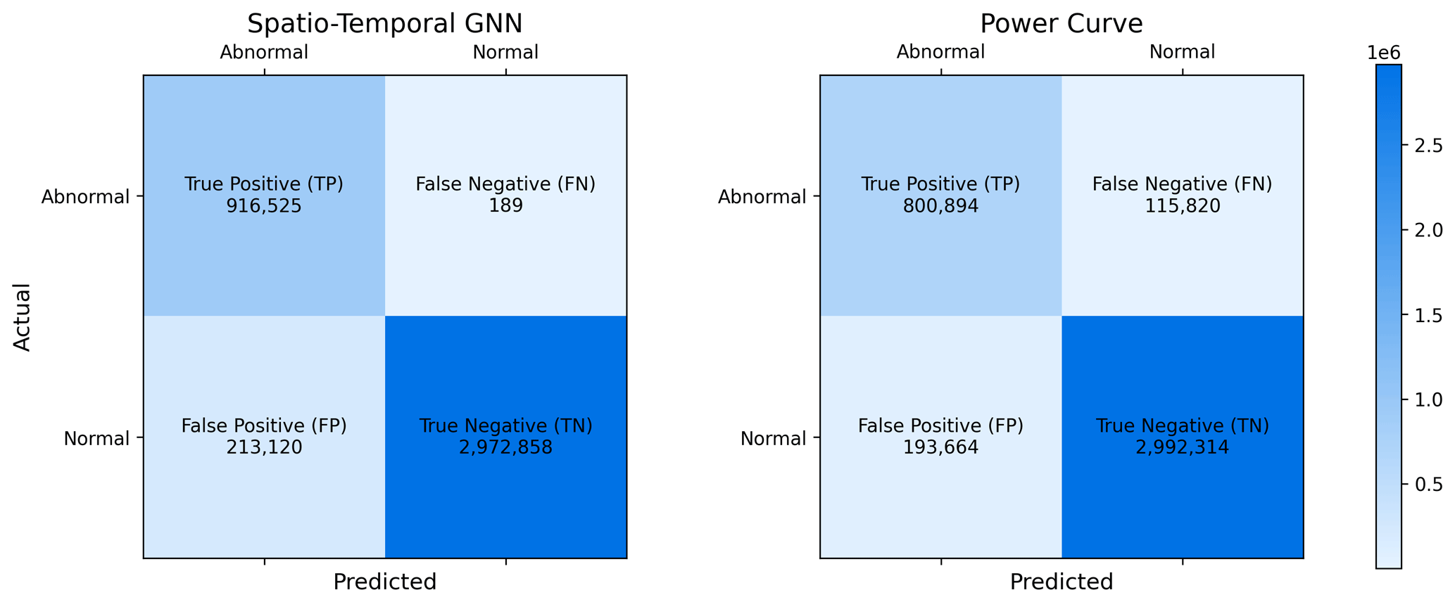
Figure 4 Confusion matrix for NBM methodology using the spatio-temporal GNN and the power curve model. Each entry represents the number of correctly predicted timestamps during the evaluation period.

With the spatio-temporal GNN, the majority of data points in the confusion matrix fall into the categories of true positives or true negatives, representing the desired outcomes of the methodology. Notably, the model achieves a very low false negative rate, with only 0.02 % of power loss events going undetected. The few false negatives that do occur correspond to turbine shutdowns under extremely low wind conditions, where the potential power is nearly zero, and the prediction error does not exceed the threshold for abnormal behavior. The remaining data points are false positives, representing instances where the model flagged anomalies without corresponding evidence in the status logs. In contrast, the power curve binning method exhibits a significantly higher false negative rate, leaving approximately 12.6 % of power loss events undetected. While this method yields fewer false positives, as discussed in Sect. 4.4, the absence of an exhaustive record of all power loss events prevents us from drawing meaningful conclusions from this metric.

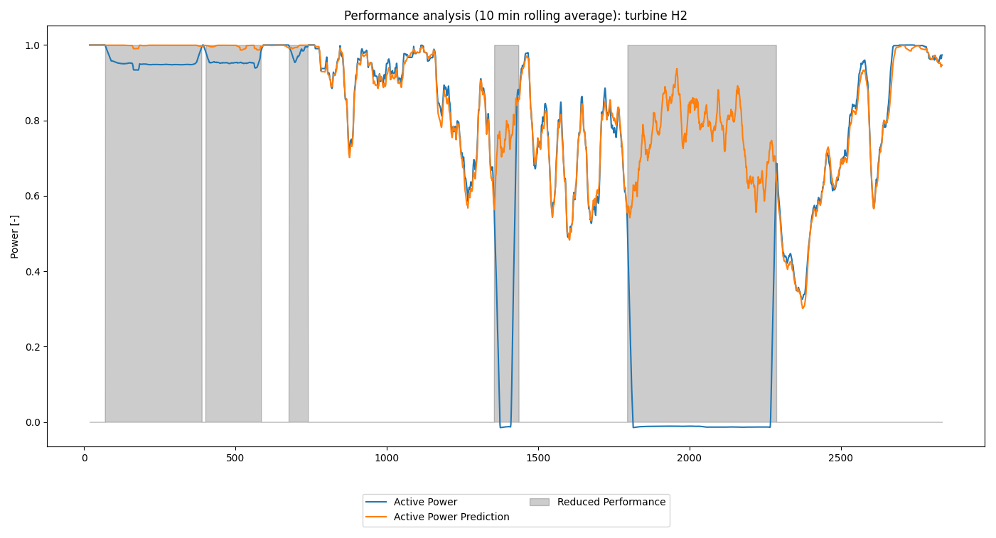
Figure 5 Performance analysis case study. A time series of the turbine's active power and the spatio-temporal GNN's prediction, smoothed using a 10 min rolling average. The gray zones indicate abnormal performance events and are annotated using the NBM.

4.3 Analysis of a known power loss event

To further demonstrate the efficacy of our methodology in detecting power loss events, we conducted a detailed case study. Figure 5 illustrates a 24 h period during which the active power output of a wind turbine, along with the corresponding predictions by the spatio-temporal GNN model, were analyzed. This period was chosen arbitrarily because it includes known loss events, making it suitable for demonstrating the model's ability to detect such anomalies. During this period, five loss events were detected, as indicated by the gray-shaded areas. Since these events were confirmed by the status logs, they were categorized as true positives.

The first three power loss events exhibit similar characteristics, as do the last two. In the first three events, the turbine's active power remains at around 95 % of its rated capacity, whereas the prediction model suggests that the turbine should be operating at full capacity. These power loss events are briefly interrupted by periods where the active power returns to the rated level. This pattern is consistent with a known curtailment strategy employed by the wind farm, where high wind speeds generate more power than can be transmitted to the grid, necessitating the partial curtailment of the farm's output.

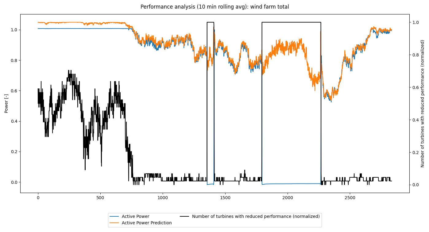
Figure 6 Performance analysis case study. A time series of the wind farm's total active power and the spatio-temporal GNN's prediction, smoothed using a 10 min rolling average. The black line denotes the number of turbines with reduced performance, as detected by the NBM.

Figure 6 provides a broader perspective by aggregating data from individual turbines to represent the total active power output and the spatio-temporal GNN model's predictions for the entire wind farm. Additionally, the figure displays the number of turbines experiencing power loss events as detected by the NBM method.

During the period encompassing the first three power loss events, the total active power of the farm remains at its maximum capacity, while the predicted power exceeds this level. During this time, the farm controller actively manages the total output by curtailing certain turbines to avoid exceeding grid-capacity limits.

The last two events follow a different pattern, where the turbine shuts down completely while the prediction model continues to forecast non-zero active power. These significant prediction errors enable the NBM method to effectively detect these power loss events. An examination of the total wind farm data reveals that these shutdowns affected the entire farm, not just individual turbines. While a detailed root cause analysis is beyond the scope of this study, these events demonstrate the utility of our methods in identifying and analyzing power loss events. Furthermore, the ability to predict potential power output during these events provides valuable insights into the magnitude of power losses and their associated revenue impacts.

4.4 Analysis of unknown power loss events

It is worth noting that there is a considerable number of false positives. This outcome is partially expected, given the lack of an exhaustive list of status logs containing all power loss events. However, upon closer examination, two wind turbines stand out for having a significantly higher number of false positives compared to the rest of the wind farm.

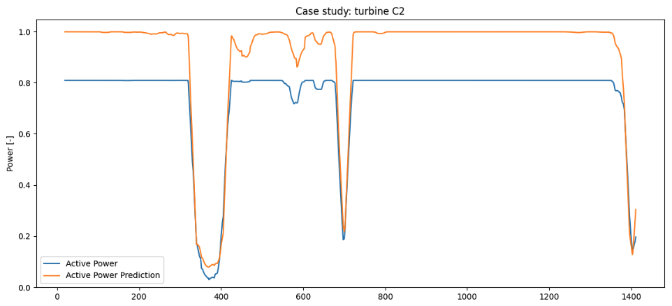
Figure 7 Performance analysis case study. A time series of the turbine's active power and the spatio-temporal GNN's prediction, both smoothed with a 10 min rolling average, over a 2 d period.

The first case involves a wind turbine that consistently produces around 80 % of its rated power, as shown in Fig. 7. A brief analysis indicates that this is a deration of an individual turbine in the farm, a detail not captured in the available status logs. Since derations often result from spontaneous operator decisions and are typically not well documented in status logs, the automated post hoc detection of these events is valuable for ensuring accurate availability data. This enables operators to more precisely assess key performance indicators like turbine availability to quantify revenue losses due to derated turbines and to verify compliance according to required performance standards.

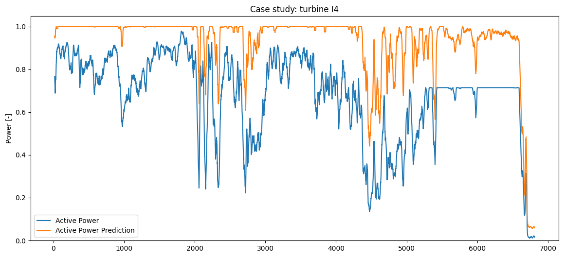
Figure 8 Performance analysis case study. A time series of the turbine's active power and the spatio-temporal GNN's prediction, both smoothed with a 10 min rolling average, over a 5 d period.

The second case is more complex and is depicted in Fig. 8. In the days leading up to a maintenance event, we observed large and continuous discrepancies between the turbine's active power output and the model’s predictions. The turbine consistently produced less energy than expected, followed by a deration and eventual shutdown. Upon investigating this previously unknown power loss event through historical logs, we discovered issues with the wind sensors on that turbine. These issues led to inconsistent pitch behavior, affecting the power output, as pitch regulation is dependent on accurate wind speed measurements from the sensors.

5 Discussion

As demonstrated in Sect. 4, our GNN-based power prediction models consistently outperform traditional methods for both predicting power during normal operations and detecting abnormal events. The spatio-temporal GNN's unique ability to incorporate lagged input feature values introduces an additional temporal dimension, enabling it to identify and exploit trends over time. This temporal insight proves particularly valuable in capturing dynamic wind condition changes, such as fluctuations in wind speed and direction, while also smoothing out noise in high-frequency SCADA data.

Our findings show that the spatio-temporal GNN excels in power prediction, especially under waked conditions. Unlike the power curve binning method and a simple MLP, which struggle to accurately predict energy ratios in these scenarios, the spatio-temporal GNN achieves significantly greater accuracy. This consistency between model predictions and the intuitive understanding of turbine interactions under varying wind conditions highlight the model's capability to effectively capture the intricate dynamics of wake interactions within the wind farm.

Additionally, we validated our model in scenarios lacking ground truth data by using them to detect anomalies through deviations from expected behavior. The GNN-based methodology demonstrated remarkable proficiency in detecting nearly all power loss events, whereas the power curve binning method failed to identify a substantial portion of these anomalies.

The superior performance of the GNN model emphasizes the advantage of representing the wind farm as a graph. In this representation, each turbine not only considers its local measurements but also incorporates information from neighboring turbines through message passing, capturing complex spatial dependencies across the wind farm. By integrating wind farm topology into power predictions and learning local features, we anticipate that this model is transferable to new and unseen wind farms. However, this claim needs further investigation.

Despite its advanced capabilities, developing and training the spatio-temporal GNN requires minimal effort. A single model suffices for an entire wind farm, and training time ranges from minutes to a few hours on a graphics processing unit (GPU), depending on the selected hyperparameters. This efficiency, combined with its predictive power, makes the GNN-based approach a practical and scalable solution for wind farm power prediction and anomaly detection.

6 Conclusions

Our study introduces a robust and innovative approach for predicting the potential power output of wind turbines in a wind farm at a 30 s temporal resolution by leveraging the spatial and temporal dynamics of the wind environment. By modeling the wind farm as a graph and using graph neural networks (GNNs) to aggregate information from neighboring turbines, we significantly improve prediction accuracy compared to traditional power curve methods. The addition of a temporal component further enhances the model's ability to capture and leverage temporal patterns in the data, achieving reductions of 30.3 % and 30.5 % in mean absolute error (MAE) and mean absolute percentage error (MAPE), respectively, compared to the power curve method.

The spatio-temporal GNN demonstrates remarkable agreement with SCADA-derived energy ratios across the full range of wind directions, achieving a weighted average error of 0.0373, an improvement of approximately 57.4 % compared to the power curve binning method. Notably, the model excels under waked conditions, where the power curve and multilayer perceptron (MLP) models exhibit higher error rates.

Beyond power prediction, our methodology shows exceptional utility in detecting turbine underperformance and power loss events. Integrated into a normal behavior model (NBM) framework, the spatio-temporal GNN achieves a remarkably low false negative rate of just 0.02 %, identifying nearly all power loss events accurately. In contrast, the power curve binning method leaves approximately 12.6 % of such events undetected, underscoring the practical advantages of the GNN-based approach. The case studies presented validate the model's effectiveness in detecting grid curtailments, shutdowns, individual turbine derations, and anomalous behavior, offering valuable insights into the operational performance of wind farms.

Our findings confirm the scalability and practicality of the GNN approach. A single spatio-temporal GNN model suffices for an entire wind farm, requiring minimal computational effort and delivering significant accuracy improvements.

Future work could aim to improve model accuracy by incorporating additional environmental factors and expanding its application to different wind farms. Developing a model that operates effectively across multiple wind farms presents a promising research direction. Achieving this, however, requires further efforts in data standardization and the consolidation of varying data formats across wind farms. In this context, the use of ontologies and taxonomies (e.g., reference designation system for power plants (RDS-PP)), could facilitate consistent data integration. Furthermore, we plan to explore the use of this power prediction framework in wind farm control. Accurate predictions of potential power output are critical for optimizing power setpoints; however, such optimization must also consider the load spectrum to balance energy production and turbine longevity (Verstraeten et al., 2019; Nejad et al., 2022).