the Creative Commons Attribution 4.0 License.
the Creative Commons Attribution 4.0 License.
Simulations suggest offshore wind farms modify low-level jets
Daphne Quint
Julie K. Lundquist
David Rosencrans
Offshore wind farms are scheduled to be constructed along the East Coast of the US in the coming years. Low-level jets (LLJs) – layers of relatively fast winds at low altitudes – also occur frequently in this region. Because LLJs provide considerable wind resources, it is important to understand how LLJs might change with turbine construction. LLJs also influence moisture and pollution transport; thus, the effects of wind farms on LLJs could also affect the region’s meteorology. In the absence of observations or significant wind farm construction as yet, we compare 1 year of simulations from the Weather Research and Forecasting (WRF) model with and without wind farms incorporated, focusing on locations chosen by their proximity to future wind development areas. We develop and present an algorithm to detect LLJs at each hour of the year at each of these locations. We validate the algorithm to the extent possible by comparing LLJs identified by lidar, constrained to the lowest 200 m, to WRF simulations of these very low LLJs (vLLJs). In the NOW-WAKES simulation data set, we find offshore LLJs in this region occur about 25 % of the time, most frequently at night, in the spring and summer months, in stably stratified conditions, and when a southwesterly wind is blowing. LLJ wind speed maxima range from 10 m s−1 to over 40 m s−1. The altitude of maximum wind speed, or the jet “nose”, is typically 300 m above the surface, above the height of most profiling lidars, although several hours of vLLJs occur in each month in the data set. The diurnal cycle for vLLJs is less pronounced than for all LLJs. Wind farms erode LLJs, as LLJs occur less frequently (19 %–20 % of hours) in the wind farm simulations than in the no-wind-farm (NWF) simulation (25 % of hours). When LLJs do occur in the simulation with wind farms, their noses are higher than in the NWF simulation: the LLJ nose has a mean altitude near 300 m for the NWF jets, but that nose height moves higher in the presence of wind farms, to a mean altitude near 400 m. Rotor region (30–250 m) wind veer is reduced across almost all months of the year in the wind farm simulations, while rotor region wind shear is similar in both simulations.
- Article
(4189 KB) - Full-text XML
- BibTeX
- EndNote
The U.S. Government and the publisher, by accepting the article for publication, acknowledge that the U.S. Government retains a nonexclusive, paid-up, irrevocable, worldwide license to publish or reproduce the published form of this work, or allow others to do so, for U.S. Government purposes.
Wind farms off of the coast of the northeastern US are expected to grow rapidly in the next few years, with goals to reach a capacity of 30 GW by 2030 and 110 GW by 2050 (U.S. Department of Energy, 2023). Wind turbines will be grouped into clusters within the 27 active wind farm lease areas that span the mid-Atlantic outer continental shelf; the current status of lease areas can be found at https://www.boem.gov/renewable-energy/lease-and-grant-information (last access: 10 December 2024).
The considerable wind resource in this region derives not only from the faster wind speeds over open water but also from the frequent occurrences of low-level jets (LLJs) here. An LLJ is a region of relatively fast winds at low altitudes in the atmosphere. LLJs occur globally (Rife et al., 2010) and provide considerable wind resource due to their fast wind speeds (Vanderwende et al., 2015; Doosttalab et al., 2020). However, LLJs can also cause excess wear and tear on wind turbine blades (Kelley et al., 2006; Gutierrez et al., 2016). The fast wind speeds, wind shear, and wind veer associated with LLJs can affect the energy production of a wind farm (Chatterjee et al., 2022), especially when LLJs interact with complex terrain (Radünz et al., 2022).
Several mechanisms can induce the formation of LLJs. LLJ formation was first described for the onshore environment. As described by Blackadar (1957) and Bonner (1968), LLJs are initiated by the evening cessation of turbulence near the surface. This release of turbulent stresses or frictional decoupling leads to an acceleration, taking the form of an inertial oscillation, which in turn results in a jet structure in low-level winds. Baroclinicity, due to sloping terrain (Holton, 1967) or frontal dynamics, can supplement the inertial oscillation mechanism. Several climatologies of onshore LLJs explore the roles of these various mechanisms and resulting impacts on jet characteristics, such as the maximum wind speed, the height of the wind speed maximum, and the evolution of the LLJ over the course of a night (Bonner, 1968; Whiteman et al., 1997; Banta et al., 2002; Song et al., 2005; Lundquist and Mirocha, 2008; Rife et al., 2010; Baas et al., 2009; Vanderwende et al., 2015; Smith et al., 2018, 2019). LLJs frequently cause strong wind shear and, in some cases, wind veer underneath the nose of the jet (Banta et al., 2002).
The same mechanisms (inertial oscillations and baroclinicity) result in LLJs in the offshore environment, even as winds are generally faster in the offshore environment due to the low surface roughness of the ocean. As first described in Högström and Smedman-Högström (1984), flow from land over water also experiences a frictional decoupling, leading to an acceleration and a jet structure in winds off a coast. The resulting marine LLJs are explored in more detail by Smedman et al. (1995) and Smedman et al. (1993). The frequent occurrences of LLJs in the North Sea (Dörenkämper et al., 2015; Wagner et al., 2019) arise from this mechanism. LLJs can also form in coastal regions after the cessation of sea breeze circulations, triggered by an inertial oscillation initiated when the sea breeze decays (Angevine et al., 2006). As in the onshore case, baroclinicity, in this case due to temperature contrasts between land and water in coastal regions, can amplify the LLJ. As a result, winds that allow long offshore fetch – southwesterly winds in the US East Coast wind energy regions – are associated with LLJs in the New York Bight region (Colle and Novak, 2010). Southwesterly winds occur frequently in this region and arise from geostrophic flow around persistent high pressure over the ocean and low pressure over land. This southwesterly flow brings relatively warm air from the south over colder mid-Atlantic waters, creating stable conditions suitable for frictional decoupling and jet formation. At night during the summer, radiative cooling on sloping terrain to the west creates an air temperature gradient near the surface, with higher temperatures over the sea. This baroclinicity impacts the gradient of the geostrophic wind in the vertical, resulting in a thermal wind that increases with height. The LLJ is formed at the local maximum in wind speeds associated with this thermal wind gradient (Holton, 1967; de Jong et al., 2023). Additionally, low-pressure systems moving over land to the west can result in a tightening of the pressure gradient and a stronger southwesterly wind offshore (Strobach et al., 2018).
Previous studies have characterized offshore LLJs in this region from observations, albeit for case studies during specific field campaigns. South of Martha's Vineyard, Mahrt et al. (2014) observe low-level wind maxima over 2 d, associated with developing stable stratification; the altitude of the wind speed maximum is higher with stronger stability. (These observations were collected with the Long-EZ aircraft, a light pusher aircraft with a rear-mounted engine and a small, low-drag airframe.) Farther north, in the Gulf of Maine, Pichugina et al. (2017) use a ship-based scanning lidar to assess LLJ profiles during an intensive 1-month deployment, finding that LLJs occur 63 % of the time, with maximum jet heights occurring up to 600 m, although the average jet height is approximately 155 m above the surface.
More recently, offshore floating lidar buoys enable longer-term characterization of LLJs but at altitudes constrained by lidar capabilities. In an analysis of LLJs at two floating lidar buoys, Debnath et al. (2021) find that LLJs occur primarily when a southwesterly wind is blowing, in the spring and summer months, and when there is a positive air–sea temperature difference. Similarly, Aird et al. (2022) identify LLJs in several groups along the East Coast and find LLJs are preferentially aligned with the nearest coastline and occur primarily in the warm season with a peak in June and when air temperatures are cooler offshore. Both find that LLJs often occur at heights relevant to wind energy. Floating lidar buoy studies are limited to the lowest 220 m accessible by lidar measurements.
The interaction of LLJs with wind farms in the offshore US East Coast regions has not yet been investigated, despite the occurrences of LLJs in this region and the planned offshore development. In addition to providing wind resources, LLJs can affect the recovery of wind farm wakes, which result from clusters of turbines. To make maximum use of the wind lease areas, wind turbines are arranged in large clusters that may interact with each other. Large arrays of turbines produce wakes – regions of slower wind and more turbulent flow downwind of the turbines – that can propagate for tens of kilometers (Hasager et al., 2006; Platis et al., 2018; Rosencrans et al., 2024). The wake wind speed reduction downwind of the wind farm can reduce power output (Nygaard, 2014; Lundquist et al., 2019). Wakes recover more slowly during stably stratified conditions (Lundquist et al., 2019; Platis et al., 2022; Cañadillas et al., 2022). Wakes also recover faster in the presence of a low-height LLJ profile, which improves the performance of turbines downwind (Gadde and Stevens, 2021). A simulation study of the interactions of one LLJ with wind farms in the North Sea (Larsén and Fischereit, 2021) suggests that the position of the nose of the LLJ and the resulting shear between the surface and the LLJ nose are modified by the wind farms and their wakes.
Our research broadens this understanding by using a yearlong data set of numerical weather prediction simulations to quantify the expected impact of wind farms on LLJs offshore. We assess the temporal and spatial variability of occurrences of LLJs and the characteristics of LLJs, such as their maximum wind speed, height of wind speed maximum, and associated wind shear and wind veer. We then assess how wind turbine wakes influence these LLJ characteristics. Here, however, we compare characteristics of LLJs both with and without wind farms present based on numerical simulations, which enable assessment of LLJ structures that occur above the height of profiling lidars. Understanding the interaction between wind farms and LLJs is crucial for accurately forecasting energy production and facilitating grid integration of renewably generated electricity.
To understand how wind turbines may modify LLJs, we compare the Weather Research and Forecasting (WRF) model (Skamarock et al., 2021) simulations of Rosencrans et al. (2024) that represent conditions in the region from September 2019 to September 2020. Three of these simulations include different wind farm layouts, and one simulation does not include any wind farms in the model. In Sect. 2, we present the data set used and the locations of interest. In Sect. 3, we describe our definition of a low-level jet and our detection methods. Section 4 includes quantification of LLJ occurrences, seasonal and diurnal cycles, jet heights, rotor region wind veer and wind shear, and wind direction for both the no-wind-farm (NWF) and wind farm (WF) simulations. We discuss an extreme LLJ case that occurs in both the lidar observations and the simulation data set in Sect. 5. We conclude and summarize our results in Sect. 6. The results of this assessment are neither intended to make nor intended to be suitable for making commercial judgments about specific wind projects.
2.1 Model data set
In this study, we use the NOW-WAKES data set described in Rosencrans et al. (2024) and Bodini et al. (2024), which quantifies the effects of wind farm wakes on energy production. Full details on the data set appear in Rosencrans et al. (2024), but a brief summary is provided here. The data set is created using WRF version 4.2.1 and the wind farm parameterization of Fitch et al. (2012). We use the innermost domain (domain 2) of the two nested domains, which is bounded by 37.389–42.137° N and 76.208–64.977° W (Fig. 1). Domain 2 has a 2 km horizontal resolution and a 10 m vertical resolution near the surface with stretching aloft. There are 34 vertical levels in the lowest 2000 m and 29 in the lowest 750 m. These simulations without wind farms are validated in comparison to floating lidar observations at two locations in the domain (Rosencrans et al., 2024), with a slow bias of less than 0.5 m s−1. The period from 1 September 2019 at 00:00 UTC to 31 August 2020 at 23:50 UTC provides a temporal resolution of 10 min; we use hourly time steps for our analysis.
Three simulations consider three different wind farm layouts, and one simulation does not include any wind farms in the model (Table 1). The first wind farm layout includes only turbines in one specific lease area, referred to as “ONE” here and in Rosencrans et al. (2024). The second layout considers turbines in all lease areas, and the third considers all turbines in both the call areas and the lease areas as of September 2019. Figure 1 shows the locations of the wind turbines for each of these simulations. The turbines introduced in these simulations are 12 MW with a rotor disk extending from 30 to 245 m and a hub height of 138 m. To assess the effect of including or not including turbine-generated turbulent kinetic energy (TKE), separate simulations with 0 % and 100 % added TKE are available, but we consider only the 100 % TKE simulations. Note that the simulation for the call areas only lasts 4 months (September and October of 2019 and July and August of 2020) instead of the full year as in the other simulations due to computational limitations.
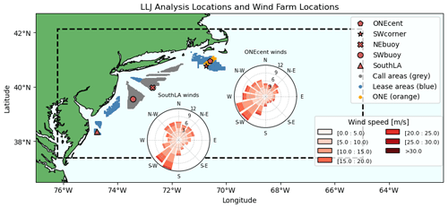
Figure 1 Simulation domain including turbine locations and regional wind roses. The five locations analyzed are in red with a black outline. The turbine locations for each of the three wind farm layouts are shaded, with ONE in orange, lease areas in blue, and call areas in gray. The domain 2 boundary is outlined with the dashed black line. The wind roses show the wind speed (shading) and direction (angle) at 130 m for 1 year at ONEcent (top right) and at southLA (bottom left). The distance from the center of the plot indicates the percentage of values in each bin.
2.2 Locations of detailed study
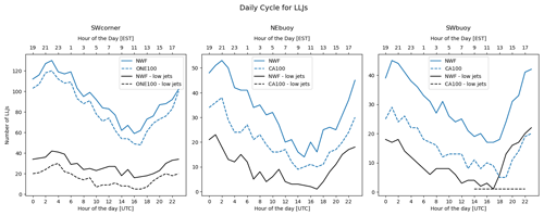
We focus on five locations in the vicinity of the ONE area, namely call areas and lease areas (Fig. 1). Two of these locations are discussed in detail (ONE centroid (ONEcent) and southern lease area (southLA) centroid), while figures for the other three locations (SW corner of ONE (SWcorner), NEbuoy, and SWbuoy) can be found in the Appendix. We focus on ONEcent and the southLA centroid because they represent the two geographic extremes of the data set. Differences between the no-wind-farm (NWF) and the wind farm (WF) simulations diminish with distance from the wind farm, so locations on land are not addressed here. The ONEcent and SWcorner locations are analyzed using the ONE-only simulation (ONE100). The locations of two floating lidar buoys (NEbuoy and SWbuoy) are analyzed using the call area simulation (CA100). The southLA centroid is analyzed using the simulation including all lease areas (LA100). Throughout the paper, we refer to wind farm (WF) simulations, and the appropriate simulation depends on the location as specified in the rightmost column of Table 1.
2.3 Additional locations
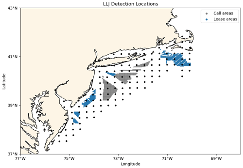
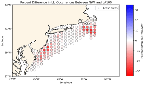
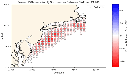
To assess the geographic variability of LLJs, LLJs are also assessed at each hour from 1 September 2019 to 31 August 2020 at each of the points in Fig. 2 using the same NOW-WAKES data set as described above. Analysis of LLJs at these locations quantifies the spatial variability in the region. The 126 points are spaced approximately 26 km apart, excepting any points on land.
3.1 LLJ detection
To identify LLJs in the simulations described above, we follow the established methodology described by Vanderwende et al. (2015), based on the foundational LLJ analysis of Bonner (1968) and Whiteman et al. (1997). This approach is also used by Song et al. (2005). However, we do include slight modifications for the offshore environment. LLJs are detected if the maximum wind speed occurs in the lowest 750 m of the atmosphere and is at least 10 m s−1. The wind speed reduction above this wind speed maximum (the nose of the jet, Banta et al., 2002) must be at least 3 m s−1; we consider heights up to 2 km for our analysis. Given the difference in mechanisms offshore and onshore (smaller force of friction, leading to weaker super-geostrophic acceleration), we use a smaller shear threshold than in Vanderwende et al. (2015). Several other approaches for identifying LLJs appear in the literature, often designed specifically for the features of the instrument platform used (i.e., Nunalee and Basu, 2014, use radar wind profiler data that offer observations in deep layers but lack measurements in the lowest 100 m). Many of the recent developments are designed for relatively shallow profiling lidar observational data sets rather than deeper observational data sets (from scanning lidar, radar wind profilers, or radiosondes) or modeling sets used here. No consistent formulation currently exists, but several of the shallow approaches are summarized in Sheridan et al. (2024), including those of Kalverla et al. (2019) and Hallgren et al. (2020).
Further, given the relevance of LLJs occurring within the rotor layer (Gadde and Stevens, 2021), we also define very low level jets (vLLJs) that, in addition to the above criteria, must have a jet nose height below 260 m. vLLJs occur at heights more relevant to wind energy than LLJs higher in the atmosphere, and, as shown below, their interactions with wakes are different from LLJs with nose heights at higher altitudes.
3.2 LLJ classification
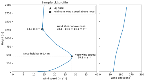
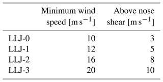
When an LLJ is identified, it is given a classification from LLJ-0 to LLJ-3 based on wind speed and wind shear values, as described in Table 3 and as seen in an LLJ-3 profile (Fig. 3). This classification pattern follows that of Vanderwende et al. (2015) and Whiteman et al. (1997). These values best define the magnitude of the LLJ and help to determine the potential impact on wind energy.
3.3 Stability calculation
LLJs onshore tend to occur in stably stratified conditions. To look for a similar relationship here, we calculate the Obukhov length (L):
where u* is the friction velocity, θv is the virtual potential temperature, κ is the von Kármán constant of 0.4, g is gravitational acceleration, and is the vertical turbulent surface heat flux. Values between 0 and 500 m are considered stably stratified conditions, and values from −500 to 0 m are considered unstable. Values outside of this range are considered neutral (Gryning et al., 2007; Sathe et al., 2011).
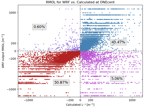
Although L−1 (referred to as RMOL) is an available output from the WRF simulations, we instead calculate L using Eq. (1) and WRF output values of UST (friction velocity) and HFX (surface heat flux). The value of RMOL output by WRF is calculated in the surface layer scheme, whereas the value of the heat flux is calculated afterward in the land surface module and so may be different from the value used in the surface layer scheme (Joseph B. Olson, personal communication, 2023). The planetary boundary layer (PBL) scheme, which induces the winds, responds to the value of the heat flux output by the land surface module, so the value of L−1 calculated with Eq. (1) is more relevant to the winds.
RMOL and L−1 can differ. When comparing the calculated values of L to the WRF output value of RMOL at ONEcent over a year of the NWF simulations, we found that the stability classifications (stable, unstable, or neutral) disagree 5.66 % of the time at ONEcent (Fig. 4).
3.4 Data set validation for LLJs
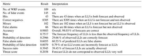
To assess the skill of WRF in simulating LLJs, we treat this case as a dichotomous forecast: an LLJ either occurs or does not. We compare WRF simulation results to observations at the E06 floating lidar, which is located at 39.55° N, 73.43° W. The profiling lidar includes horizontal wind speed and direction data for 10 vertical levels from 18 to 198 m, with an interval of 20 m. For each of the 8516 h of the year that the lidar is operational, we apply a modified LLJ detection algorithm to both data sets and compare the frequency and timing of the occurrences of LLJs. We treat each time profile separately and do not consider the duration of LLJ events or require continuity of LLJ events. Given the shallow layer of observational data available and the fact that many LLJs occur above the highest lidar level, we reduce the requirement for the wind speed reduction above the nose threshold from 3 to 1 m s−1. LLJs are relatively rare in this layer of the atmosphere: of the 8516 h analyzed, 145 events are identified by the lidar, and 109 are identified by WRF.
We first follow the validation used in Aird et al. (2022), which compares the mean LLJ profile and the monthly distribution of LLJs for both data sets (Fig. 5). Mean LLJ wind speeds and standard deviations for each level are similar between WRF and lidar above 100 m. Below this, WRF tends to have faster wind speeds, with a maximum difference of around 2 m s−1 near the surface. Standard deviations are also slightly larger near the surface in the WRF data set. Both data sets show a mean nose height of just over 100 m and mean nose wind speed of around 13 m s−1. Both data sets also have a similar seasonal cycle, with peaks in June and low occurrences from August to February. The largest differences between both data sets occur from January to April, with April having around a 5 % difference in LLJ occurrences.
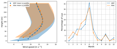
Figure 5 (left) Mean LLJ profile for WRF (blue circle) and lidar (orange diamond), with shading for the 1 standard deviation range. Both LLJs are calculated at the E06 floating lidar during the same time period.
We also assess how the timing of LLJs compares between WRF and lidar by considering each individual hour of the year. We determine the accuracy, bias, probability of detection, false alarm ratio, probability of false detection, success ratio, and threat score using LLJ data from September 2019–September 2020 (Table 4). This approach is also used by Kalverla et al. (2019), Hallgren et al. (2020), and Sheridan et al. (2024). Metrics in the last seven rows of the table are calculated using the hits, correct negative, misses, and false alarm metrics defined in the previous four rows. Because of the rarity of these events, the accuracy and probability of false detection scores can be misleading due to the high number of true negative results identified in both the model and the observations. WRF has fewer events overall, corresponding to a bias of less than 1. WRF tends to have higher LLJ nose heights, which may not be detectable by the lidar. This tendency could lead to fewer events detected overall in the WRF simulations. WRF performs poorly in the probability of detection, false alarm ratio, success ratio, and threat score metrics due to the high occurrence of misses and false alarms. While WRF profiles often match lidar profiles well, there are times when WRF misses. In Fig. 6a, the WRF profile matches the lidar profile well. In panel b, WRF does not simulate conditions below 200 m well. The center panel demonstrates a case where WRF has a similar profile to the lidar but a nose height that is too high. Within the lowest 200 m of the atmosphere, WRF does not have an LLJ due to insufficient shear above the nose. When we instead consider a 400 m layer, an LLJ profile can clearly be identified.

Figure 6 Wind profiles for WRF (blue) and lidar (orange) on 15 May 2020 at 21:00 UTC (a), 15 May 2020 at 05:00 UTC (b), and 29 April 2020 at 06:00 UTC (c). Wind speed is on the x axis, and height above the surface is on the y axis. A zero in the legend indicates that an LLJ is not identified in the lowest 200 m of the atmosphere, and a 1 indicates that an LLJ is identified. All profiles are at the E06 floating lidar buoy at 39.55° N, 73.43° W.
WRF does not closely match the lidar observations when considering each hour individually, as we identified many misses and false alarms, although the data set used here follows best practices for simulating LLJs using WRF. Previous studies recommend a 2 km resolution in the inner domain, a large number of vertical levels in the boundary layer, ERA5 reanalysis data for initial and boundary conditions, and use of the Mellor–Yamada–Nakanishi–Niino (MYNN) PBL scheme (Nunalee and Basu, 2014; Wagner et al., 2019; Kalverla et al., 2019; Siedersleben et al., 2018; Tay et al., 2021). Other studies also use WRF to simulate LLJ events and also find variable agreement between WRF simulations and lidar observations (Colle and Novak, 2010; Vanderwende et al., 2015; Larsén and Fischereit, 2021; Aird et al., 2022).
It is difficult to validate the performance of WRF due to limited observational data. The lidar can only provide validation for heights up to 200 m, but LLJs often occur higher than this (Aird et al., 2022; Vanderwende et al., 2015; Zhang et al., 2006). Our study aims to explore the variability of LLJs at heights relevant to wind energy, and WRF is currently the best option given the limitations of profiling lidars. Results in Fig. 5 show that WRF performs reasonably well in characterizing LLJs on larger timescales.
4.1 LLJ occurrences
In the NWF simulation, LLJs occur about 25 % of the time at each of the five locations. The ONEcent location has the most LLJs (26 % of the time), and the SWbuoy has the fewest occurrences (25 % of the time). Level 0 and 1 jets occur most frequently, while the faster level 2 and 3 jets are rarer (Fig. 7).
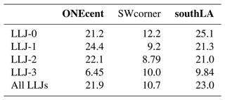
At all locations, LLJs occur less frequently when wind farms are present (Fig. 7). The southLA location has the largest reduction in LLJs, with a 23 % overall decrease (so that LLJs occur only 19.5 % of the time), followed closely by the ONEcent location with a 21 % overall reduction (so that LLJs occur only 20.3 % of the time). LLJs at the SWcorner site are reduced significantly less in the WF simulation, with 10.7 % fewer LLJs in the WF simulation than in the NWF simulation. The disparity between the ONEcent and SWcorner sites likely occurs because there are few turbines upwind of the SWcorner site when the frequent southwesterly winds are blowing. When wind farms are present, level-3 jets are reduced less than for level-0, level-1, and level-2 jets at the ONEcent and southLA sites, with reductions of 6.45 % and 9.84 %, respectively (Table 5). (The NEbuoy and SWbuoy sites do not appear in Table 5 because only 4 months of data is available for those two sites.)
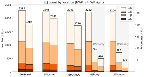
Figure 7 LLJ occurrences at each of the analyzed locations out of the 8784 possible hours. The text on top of each bar refers to the total number of hours that LLJs occur at that location. The no-wind-farm counts are on the left, and the wind farm counts are on the right. The LLJ category is shaded. Note that data from the NEbuoy and the SWbuoy include only July, August, September, and October (JASO) for the wind farm simulation, while the other three locations are for 1 full year. At the NEbuoys and SWbuoys, the full year for the NWF simulation is also included on the far left. The two bars on the right are for the NWF and WF simulations for JASO only.
Table 5Percent reduction in LLJs between the NWF and WF simulations for each classification at three locations with a full year of data.
We find similar results for the array of LLJ points across the region (Figs. 8, 9, 10). In the NWF simulation, LLJs occur between 14 % and 27 % of the time, with most locations experiencing LLJs around 25 % of the time. Locations far from any wind turbines see similar rates of LLJ occurrences in both the NWF and the LA100 simulations. Points in the vicinity of wind farms see up to a 30.5 % reduction in LLJ occurrences in the lease area simulation and up to a 49.2 % reduction in the call area simulation.
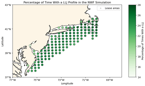
Figure 8 The percentage of times with an LLJ profile in the NWF simulation is shaded in green. Wind lease areas are shaded in gray in the background.
4.2 Relationship between LLJs and atmospheric stability
In the NWF simulations, LLJs occur during both stable and unstable conditions, but they occur more frequently during stable or neutral stratification (Table 6). Stable conditions can form offshore when warm air from the land flows over cooler air over the ocean. At all five sites, stable conditions occur between 37 % and 45 % of the time, but between 53 % and 63 % of LLJs occur in stable conditions. At ONEcent, the atmosphere is considered stable 44.4 % of the time, but 62.7 % of LLJs occurred during stable conditions. Neutral conditions occur 11.3 % of the time, but 13.9 % of the LLJs occur during neutral conditions (Table 6). The other four locations have similar distributions of stable versus unstable conditions for all times of the year and for times with LLJs. As noted in Quint et al. (2024), stable conditions in this region occur almost always with southwesterly winds (their Fig. 6).
Table 6Stability classification for each location for all times of the year (columns 1–3) and for times with an LLJ in the NWF simulation (columns 4–6) at each location (rows 1–5).

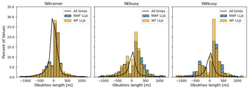
NWF and WF simulations show similar distributions in stability when LLJs occur. In both cases, very stable stratification () is more common during LLJ events than for all times of the year. Similarly, very unstable conditions () are less common during LLJs than for all times of the year (Fig. 11), and this pattern holds for the other three sites (Fig. B1). During neutral conditions (), differences between LLJs and normal conditions are small, although few LLJs occur during neutral conditions. At both the ONEcent and the southLA sites, the NWF LLJs occur slightly more often for Obukhov lengths of 0–100 m than for the WF LLJs (Fig. 11); this pattern is in contrast to the other three sites (Fig. B1).
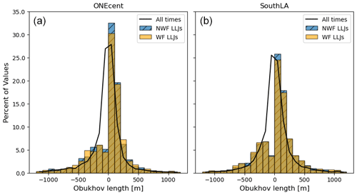
Figure 11 Distribution of Obukhov lengths at the ONE centroid (a) and the southern lease area centroid (b). Distribution of Obukhov lengths for the entire year are marked by the black line. Obukhov lengths for LLJs in the NWF simulation and WF simulation are plotted in blue with black hatches and orange, respectively. The percentages of values in each bin are represented by the y axis.
4.3 Wind speed variability of LLJ wind speed maxima
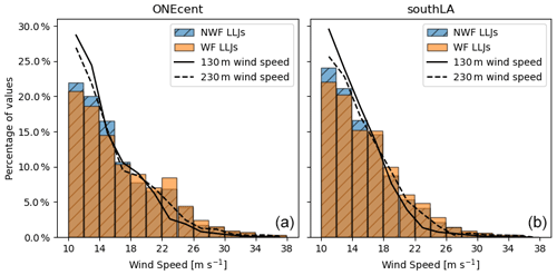
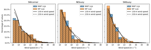
By our definition, LLJs have a minimum wind speed of 10 m s−1. LLJ maximum wind speeds in this study range from 10 m s−1 to almost 46 m s−1, but most wind speeds are slower than 30 m s−1. The LLJ occurrences in the NWF and WF simulations differ the most at slower wind speeds but are nearly identical for wind speeds faster than 20 m s−1 (Figs. 12 and C1). While wind speeds of 10–14 m s−1 occur around 25 % of the time at hub height (138 m) at each location, these wind speeds only make up around 21 % of the LLJs.
4.4 Nose heights
Nose heights range from 45 to 735 m. Mean nose heights in the NWF simulation are around 300 m at all five locations (Figs. 13 and H1), but mean jet height is slightly lower at the southLA site than at the ONEcent site. In the NWF simulation, mean nose height increases with jet classification at all locations (i.e., faster jets have higher noses) except for the NEbuoy. The southLA site also has a larger range of heights for the middle 50 % of data (Fig. 13). Nose height differences between WF and NWF simulations are much larger at the buoys, with very little overlap between the middle 50 % of data for each classification (Fig. H1), likely due to the very large wind farms in their vicinity.
When wind farms are present, the nose heights rise higher in the atmosphere as LLJs are eroded by the wind turbines (rotors in these simulations extend from 30 to 245 m). In the wind farm simulation, nose heights are all close to 450 m across all classifications, although the southLA site tends to have lower heights than the ONEcent site.
The nose height differences between the NWF and WF simulations are statistically significant. We use a two-sample t test, with 8273 values in the NWF sample (combined number of LLJ events among the five sites in the NWF simulation) and 6378 values in the WF sample (combined number of LLJ events among the five sites from the WF simulations). The mean of the NWF sample is 348.9 m, and the mean of the WF sample is 439.8 m. Both samples have similar variances and approximately normal distributions, so the t test is appropriate. For a t test with a null hypothesis that the two means are equal, we find a p value much lower than the threshold value of 0.05, so we can confidently reject the null hypothesis (that there is no significant difference between the nose heights of the NWF and WF LLJs). When analyzing each location independently, the null hypothesis can also be rejected for each location with p values much smaller than 10−4. The wind farms erode the bottom of the LLJs, pushing the nose heights higher.
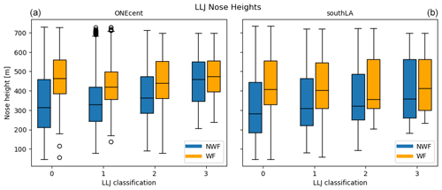
Figure 13 Nose heights by LLJ classification for NWF (blue) and WF (orange) at the ONE centroid (a) and southern lease area centroid (b).
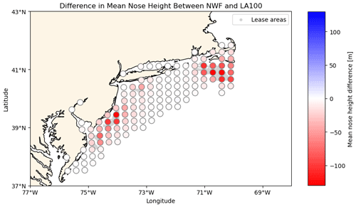
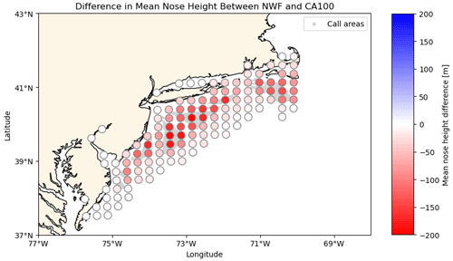
We find similar results for the array of LLJ points across the region (Figs. 14, 15, 16). Mean LLJ nose heights range from 328 to 474 m, but most locations have a mean close to 360 m. The largest increase in mean nose heights occurs at locations within a wind farm. Outside of wind farms, nose heights are similar between the NWF and LA100 or CA100 simulations. Points in the vicinity of the wind farms see up to a 129 m difference in the LA100 simulation and up to 205 m in the CA100 simulation. In general, there is a larger effect in the call area simulation, likely due to the greater number of turbines instigating a deeper internal boundary layer due to the larger wind farm.
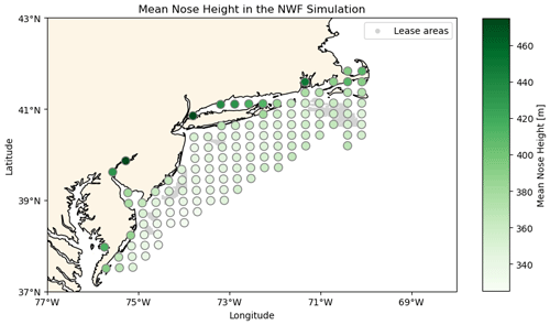
Figure 14 The mean nose height in the NWF simulation is shaded in green. The lease areas are shaded in gray in the background.
4.5 Wind direction variability of LLJ wind speed maxima
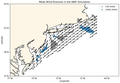
Overall, wind directions tend to be southwesterly and aligned with the coast, as are the LLJs (Fig. 17). This mode wind direction for LLJs resembles the dominant wind direction, as seen in the wind roses of Fig. 1, and the dominant wind direction of stably stratified conditions (not shown). Other investigations of observations of LLJs in this region (Colle and Novak, 2010; Debnath et al., 2021; Aird et al., 2022; de Jong et al., 2023) also document a strong preference for southwesterly flow.
4.6 Temporal variability of LLJs
4.6.1 Seasonality
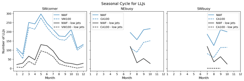
LLJs occur in all months of the year in all locations (Figs. 18 and D1). LLJs are more frequent during the spring and summer months, with peak occurrence in May. The difference between the NWF and WF simulations is also the largest during May. The locations with 12 months of data exhibit a minimum in LLJ occurrences from November to February and local maxima in March and October (Figs. 18 and D1). vLLJs follow a similar seasonal cycle, with most vLLJs occurring in the spring and summer months. In the wind farm simulation (ONE100 for ONEcent and LA100 for southLA), vLLJs are significantly eroded. At the ONEcent location, vLLJs are almost completely eroded across all months of the year. At the southLA site, vLLJs only occur in May and June when wind farms are present: the wind farms erode the vLLJs in all other months.
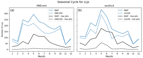
Figure 18 The number of LLJs in each month of the year is shown for the ONEcent (a) and southLA (b) locations. The NWF results are marked by a solid blue line, and the WF results are marked by a dashed blue line. vLLJs, with nose heights 260 m or below, are in black, where the solid line is for the NWF simulation, and the dashed line is for the wind farm simulation.
4.6.2 Wind direction seasonality
LLJ wind directions show seasonal variability. The mode of the wind direction varies depending on the bin size, so we consider results for bins of 1, 5, and 10° (Fig. 19). Southwesterly and northeasterly winds are most common for LLJs, but this trend varies by month and location. Southwesterly LLJs are most common in the summer months (June–September), as well as in January and March at both locations. In the month of May, LLJs vary across locations but are generally northerly or easterly, depending on the bin size. October LLJs are consistently northeasterly regardless of bin size or location. December, February, and April LLJs vary by location and bin size.
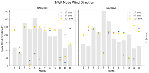
Figure 19Mode of the nose wind direction in each month for the NWF simulation at two locations for bin sizes of 1 (blue plus), 5 (pink star), and 10° (yellow circle). A histogram of the number of values is in gray. The left y axis refers to the wind direction, and the right y axis refers to the histogram.
4.6.3 Daily cycle
LLJs can occur at any time of the day at all locations but are most common between the hours of 18:00 and 02:00 local time (Figs. 20 and E1). The fewest jets occur in the morning, from 07:00 to 12:00 local time. In general, at all five locations, LLJs are twice as likely to form at night than during the day. LLJs at the southLA location persist longer into the early morning and disappear for a shorter amount of time later in the day. vLLJs follow a similar diurnal cycle to all jets but are degraded significantly when wind farms are present. vLLJs also have a less pronounced diurnal cycle compared to all jets (Fig. 20). These results are consistent with the analysis of Debnath et al. (2021), who find most LLJs also occur at night with a peak at 22:00 local time and the fewest events from 06:00 to 12:00 local time.
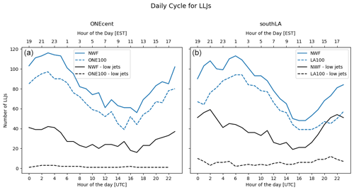
Figure 20 The number of LLJs in each hour of the day is shown for ONEcent (a) and southLA (b). The bottom x axis time is in UTC, and the top x axis is in local time (EST). The NWF results are marked by the solid blue line, and the wind farm results are in the dashed blue line. LLJs with nose heights 260 m or below are in black, where the solid line is for the no-wind-farm simulation, and the dashed line is for the wind farm simulation.
4.6.4 Wind veer seasonality
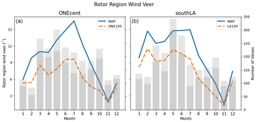
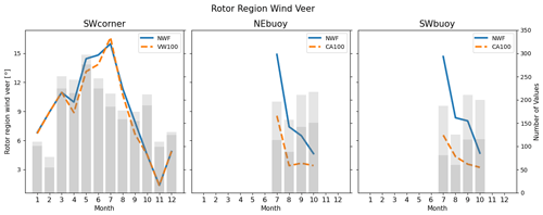
Wind veer associated with LLJs is strong in the spring and summer, reaching 15° across the rotor disk region (30–245 m), but then decreases in the fall and early winter (Figs. 21 and F1). This pattern is related to the seasonal variability in atmospheric stability. Summer months have more frequent stable conditions, and stable conditions are associated with more veer (Lundquist, 2020), especially offshore (Bodini et al., 2019, 2020). While all locations have peaks in the summer, wind veer at the southLA location is consistently stronger from February to May (February to July for ONEcent and SWcorner). Wind veer in the rotor region (30–245 m) is reduced at ONEcent and southLA when wind farms are present but with only subtle changes at SWcorner. This difference may be attributed to the fact that SWcorner is typically upwind of most turbines. The largest difference in wind veer between the WF and NWF simulations occurs from March to October, with the largest reduction in July. Wind farms induce little difference in veer from November to January (Fig. 21).
4.7 Wind shear seasonality
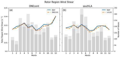
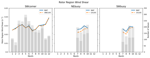
Mean wind shear in the rotor region (30–245 m) ranges from about 0.025 to 0.04 s−1 at all locations (Figs. 22 and G1). Shear values are generally constant throughout the year, but minima occur in July at most locations (in August at the SWbuoy). The primary difference between the ONEcent and southLA locations occurs in November and December, when shear decreases at southLA but increases at ONEcent. This regional variability could be due to the fact that the southern southLA location enters a more unstably stratified regime (with less wind shear) sooner in the winter than the more northern ONEcent location (with more stable conditions and more wind shear). At both locations, few differences occur between the NWF and WF shear.
On 7 February 2020, strong winds in excess of 15 m s−1 occur at the lidar site, with wind directions varying from southerly to southwesterly. According to the lidar, this event would not be considered an LLJ because of a lack of a decrease in wind speed above the height of maximum wind speed, which is at the top of the lidar range of visibility. According to the simulations, however, an extreme LLJ event does occur, with an LLJ nose wind speed of 45.8 m s−1 and a nose height of 564 m. Despite this impressive wind speed, the LLJ is classified as a level 0 event due to the low wind shear above the LLJ nose of 3.7 m s−1. While wind speeds faster than 16 m s−1 are observed from 13:00 UTC on 7 February to 08:00 UTC on 8 February, only 3 of these 20 h count as LLJ events due to the weak above-nose shear (Fig. 23).
The LLJ is likely not due to frictional decoupling but is rather associated with an anomalous wintertime severe weather outbreak that impacts the mid-Atlantic. At around 09:00 UTC on 7 February 2020, a low-pressure system over Maryland begins to rapidly intensify. By inspection of NOAA NWS surface analyses akin to Fig. 24, we can see that by 12:00 UTC, the low-pressure center reaches 980 hPa and begins to move toward the northeast. At 15:00, the low-pressure system is centered over New Jersey with a central pressure of 977 mbar. At 230 m, wind speeds at the SWcorner location reach 26 m s−1. By 18:00 – 1 h before the maximum wind speeds are observed at the SWcorner – the low-pressure system is centered over Massachusetts, forcing strong southwesterly winds offshore (Fig. 24). The system continues moving along the coast toward Nova Scotia, eventually reaching 968 mbar, while winds farther south begin to die down. While this LLJ is clearly associated with a specific synoptic event, rather than the typical inertial oscillation/frictional decoupling mechanism, it does generate very fast wind speeds that would affect the wind resource areas such that turbines would experience both strong wind shear and winds faster than cut-out wind speed.
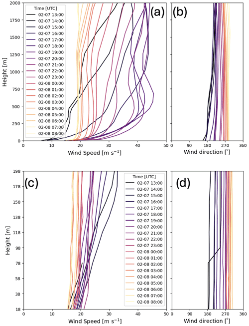
Figure 23 Wind speed (a, c) and wind direction (b, d) profiles from 7 February 2020 at 13:00 UTC to 8 February 2020 at 08:00 UTC at the lidar location from simulations (a, b) and lidar observations (c, d). Note the different vertical extent from the simulations (a, b) as compared to the limited lidar observations (c, d).
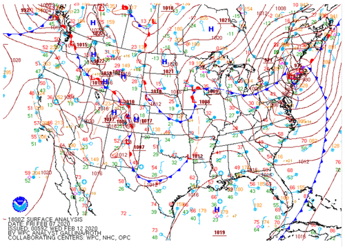
Figure 24 Surface analysis from 7 February 2020 at 18:00 UTC, 1 h before the maximum wind speeds are observed at the SWcorner location. Figure courtesy of NOAA’s National Weather Service (https://www.wpc.ncep.noaa.gov/archives/web_pages/sfc/sfc_archive_maps.php?arcdate=02/07/2020&selmap=2020020718&maptype=namussfc, last access: 10 December 2024), used with permission according to https://www.weather.gov/disclaimer (last access: 10 December 2024).
In this simulation-based study, we assess occurrences of LLJs in the US East Coast wind resource areas and how these LLJs are influenced by the presence of wind farms as they appear in numerical weather prediction simulations. We identify LLJs for a 1-year period at five different locations using WRF simulations with and without wind farms incorporated into the model. LLJs occur approximately 25 % of the time, at night, in the spring and summer months, in stably stratified conditions, and when a southwesterly wind is blowing. Modeled LLJs occur less frequently when wind farms are present in the simulations, and the jets that do occur tend to have the heights of their wind speed maxima pushed to higher altitudes in the presence of wind farms. This behavior also occurs in the case study of Larsén and Fischereit (2021) and the large-eddy simulations of Abkar et al. (2016) and Sharma et al. (2017), but this pattern is shown here to be systematic and widespread. We also document how very low level jets – LLJs with jet nose heights below 260 m – are significantly eroded by wind farms in the simulations. Consequently, we find that LLJ nose heights are generally higher in the wind farm simulations. Mean wind veer in the rotor region is reduced with wind farms, while rotor region wind shear is generally unaffected.
Because we use model simulation output, this analysis is not constrained to the lowest 200 m as studies based on profiling lidars are. While Aird et al. (2022) and Debnath et al. (2021) find lower average LLJ nose heights than we find here, our results are consistent with the scanning lidar observations of Pichugina et al. (2017) that could measure winds at higher altitudes. These results thus underscore the importance of using instruments that can probe to higher altitudes to understand the momentum available for wake replenishment by LLJs.
The seasonal LLJ climatology presented here agrees with the seasonality found in other studies on LLJs in this region. Aird et al. (2022), Colle and Novak (2010), Debnath et al. (2021), and Zhang et al. (2006) all find a peak in LLJs during the warm season and a minimum in the winter months. There is less of a consensus on the diurnal cycle of LLJs, but multiple studies, both onshore and offshore, suggest that LLJs occur more often in the early evening and at night (Zhang et al., 2006; Colle and Novak, 2010; Debnath et al., 2021). Southwesterly winds are the primary wind direction for LLJs in this region, but westerly, northwesterly, and northeasterly LLJs can also occur (Aird et al., 2022; Debnath et al., 2021; Zhang et al., 2006; Colle and Novak, 2010). LLJ studies in this region vary in terms of heights considered, but many find jets at heights relevant to wind energy. However, LLJs with noses above the rotor plane can still impact turbines due to positive wind shear below the nose. In this study, we find that vLLJs are significantly eroded by wind farms but occasionally occur at locations with fewer turbines upwind (southLA and SWcorner; see Appendix).
These findings improve our understanding of the expected energy production from offshore wind projects. While LLJs do provide significant wind resources, they can also increase loads on turbines (Kelley et al., 2006; Gutierrez et al., 2016). LLJs also impact the meteorology of the area, which influences energy demand on the East Coast. Because LLJs, and especially vLLJs, are eroded by wind farms, we can expect LLJs to exert a smaller micrometeorological influence in the vicinity of wind farms.
Several avenues of future research could further explore the variability of LLJs in this region and how they may interact with developing wind farms. The five locations focused on here are selected for their proximity to offshore wind development areas. Despite their geographic dispersal, they may not fully represent the diverse conditions along the entire US East Coast. Future research could consider a broader array of locations to better understand the spatial variability of LLJs in the region. Additionally, this study uses 1 year of simulations (selected due to the availability of lidar observations for validation of the NWF simulations). Yet, interannual variability can be consequential for wind resources (Bodini et al., 2016; Lee et al., 2018). As interannual variability cannot be considered with this 1-year data set, future studies could assess longer data sets to simulate a wider range of conditions. Other developments in modeling could also find different behavior. For example, these simulations use the MYNN PBL scheme, but other PBL schemes coupled with a wind farm parameterization, as in Rybchuk et al. (2022), may yield other insights. Ocean response to wakes may also mediate LLJ–wind farm interactions, so coupled ocean–wave–atmosphere modeling approaches, such as the approach presented in Fischereit et al. (2022), could be considered as well. Ultimately, this study and future modeling studies of LLJ–wind farm interactions await the collection of observational data sets to quantify how wind farms and LLJs affect each other.
We also analyze locations on land at Martha's Vineyard and on Long Island, where we might expect the ONE and call area wind farms to impact LLJs. We find that the NWF and WF simulations are very similar in terms of LLJ occurrence, so these locations are not included in the paper. Distance from the wind farm may play a role in these results: the south coast of the Martha’s Vineyard site is approximately 30 km from the closest part of the ONE wind farm. The closest distance of Long Island to Empire Wind I is approximately 22 km, per https://www.nyserda.ny.gov/-/media/Project/Nyserda/Files/Publications/Fact-Sheets/LSR-offshore-wind-visibility-fact-sheet.pdf (last access: 10 December 2024).
The SW corner exhibits a similar seasonal cycle to the ONE and southLA locations (see Fig. 18), where LLJs peak in May (Fig. D1). Note that vLLJs are not eroded as much here. This resistance to erosion may be because there are fewer turbines upwind of the SWcorner when a SW wind is blowing. At the buoys, with many turbines upwind, vLLJs are completely eroded.
Similar to the ONEcent and southLA locations (see Fig. 21), mean rotor region wind veer is reduced when wind farms are present at the buoys. At the SW corner, rotor region veer is similar for all months of the year (Fig. F1). Fewer turbines upwind of this location may play a role in this difference.
Similar to the ONEcent and southLA locations (see Fig. 22), mean rotor region wind shear is reduced when wind farms are present at the buoys. At the SWcorner, rotor region shear is similar for all months of the year (Fig. G1). We suspect that fewer turbines upwind of this location may play a role in this difference.
Mean nose heights are higher in the wind farm simulations at the SWcorner, NEbuoy, and SWbuoy locations. These results are in agreement with results from the ONE and southLA sites (Fig. 13). Nose height differences are much larger at the buoys, with very little overlap between the middle 50 % of data for each classification (Fig. H1).
The data set used can be obtained from https://doi.org/10.25984/1821404 (National Renewable Energy Laboratory, 2020). The code used can be found at https://doi.org/10.5281/zenodo.10993298 (Quint, 2024).
JKL conceptualized the project and acquired funding and resources for the project. DR completed the WRF simulations and provided the data set. DQ carried out the formal analysis and investigation, including developing software and carrying out the visualization, with supervision from JKL and DR. DQ and JKL prepared the initial draft. JKL, DR, and DQ reviewed and edited the paper.
At least one of the (co-)authors is a member of the editorial board of Wind Energy Science. The peer-review process was guided by an independent editor, and the authors also have no other competing interests to declare.
Publisher’s note: Copernicus Publications remains neutral with regard to jurisdictional claims made in the text, published maps, institutional affiliations, or any other geographical representation in this paper. While Copernicus Publications makes every effort to include appropriate place names, the final responsibility lies with the authors.
This work was supported by an agreement with NREL under APUP UGA-0-41026-125. This work was authored in part by the National Renewable Energy Laboratory, operated by the Alliance for Sustainable Energy, LLC, for the US Department of Energy (DOE) under contract no. DE-AC36-08GO28308. Funding was provided by the US Department of Energy Office of Energy Efficiency and Renewable Energy Wind Energy Technologies Office and by the National Offshore Wind Research & Development Consortium under agreement no. CRD-19-16351. The views expressed in the article do not necessarily represent the views of the DOE or the U.S. Government. Neither NYSERDA nor OceanTech Services/DNV have reviewed the information contained herein and the opinions in this report do not necessarily reflect those of any of these parties. A portion of computation used the Blanca Condo computing resource at the University of Colorado Boulder. Blanca is jointly funded by computing users and the University of Colorado Boulder. A portion of computation used the Summit supercomputer, which is supported by the National Science Foundation (awards ACI-1532235 and ACI-1532236), the University of Colorado Boulder, and Colorado State University. The Summit supercomputer is a joint effort of the University of Colorado Boulder and Colorado State University. A portion of this research was performed using computational resources sponsored by the DOE’s Office of Energy Efficiency and Renewable Energy and located at NREL.
This research has been supported by the National Renewable Energy Laboratory (APUP UGA-0-41026-125).
This paper was edited by Andrea Hahmann and reviewed by two anonymous referees.
Abkar, M., Sharifi, A., and Porté-Agel, F.: Wake flow in a wind farm during a diurnal cycle, J. Turbul., 17, 420–441, https://doi.org/10.1080/14685248.2015.1127379, 2016. a
Aird, J. A., Barthelmie, R. J., Shepherd, T. J., and Pryor, S. C.: Occurrence of Low-Level Jets over the Eastern U.S. Coastal Zone at Heights Relevant to Wind Energy, Energies, 15, 445, https://doi.org/10.3390/en15020445, 2022. a, b, c, d, e, f, g, h
Angevine, W. M., Tjernström, M., and Žagar, M.: Modeling of the Coastal Boundary Layer and Pollutant Transport in New England, J. Appl. Meteorol. Clim., 45, 137–154, https://doi.org/10.1175/JAM2333.1, 2006. a
Baas, P., Bosveld, F. C., Baltink, H. K., and Holtslag, A. a. M.: A Climatology of Nocturnal Low-Level Jets at Cabauw, J. Appl. Meteorol. Clim., 48, 1627–1642, https://doi.org/10.1175/2009JAMC1965.1, 2009. a
Banta, R., Newsom, R. K., Lundquist, J. K., Pichugina, Y. L., Coulter, R. L., and Mahrt, L.: Nocturnal Low-Level Jet Characteristics Over Kansas During Cases-99, Bound.-Lay. Meteorol., 105, 221–252, https://doi.org/10.1023/A:1019992330866, 2002. a, b, c
Blackadar, A. K.: Boundary Layer Wind Maxima and Their Significance for the Growth of Nocturnal Inversions, B. Am. Meteorol. Soc., 38, 283–290, https://doi.org/10.1175/1520-0477-38.5.283, 1957. a
Bodini, N., Lundquist, J. K., Zardi, D., and Handschy, M.: Year-to-year correlation, record length, and overconfidence in wind resource assessment, Wind Energ. Sci., 1, 115–128, https://doi.org/10.5194/wes-1-115-2016, 2016. a
Bodini, N., Lundquist, J. K., and Kirincich, A.: U.S. East Coast Lidar Measurements Show Offshore Wind Turbines Will Encounter Very Low Atmospheric Turbulence, Geophys. Res. Lett., 46, 5582–5591, https://doi.org/10.1029/2019GL082636, 2019. a
Bodini, N., Lundquist, J. K., and Kirincich, A.: Offshore Wind Turbines Will Encounter Very Low Atmospheric Turbulence, J. Phys. Conf. Ser., 1452, 012023, https://doi.org/10.1088/1742-6596/1452/1/012023, 2020. a
Bodini, N., Optis, M., Redfern, S., Rosencrans, D., Rybchuk, A., Lundquist, J. K., Pronk, V., Castagneri, S., Purkayastha, A., Draxl, C., Krishnamurthy, R., Young, E., Roberts, B., Rosenlieb, E., and Musial, W.: The 2023 National Offshore Wind data set (NOW-23), Earth Syst. Sci. Data, 16, 1965–2006, https://doi.org/10.5194/essd-16-1965-2024, 2024. a
Bonner, W. D.: CLIMATOLOGY OF THE LOW LEVEL JET, Mon. Weather Rev., 96, 833–850, https://doi.org/10.1175/1520-0493(1968)096<0833:COTLLJ>2.0.CO;2, 1968. a, b, c
Cañadillas, B., Beckenbauer, M., Trujillo, J. J., Dörenkämper, M., Foreman, R., Neumann, T., and Lampert, A.: Offshore wind farm cluster wakes as observed by long-range-scanning wind lidar measurements and mesoscale modeling, Wind Energ. Sci., 7, 1241–1262, https://doi.org/10.5194/wes-7-1241-2022, 2022. a
Chatterjee, T., Li, J., Yellapantula, S., Jayaraman, B., and Quon, E.: Wind farm response to mesoscale-driven coastal low level jets: a multiscale large eddy simulation study, J. Phys. Conf. Ser., 2265, 022004, https://doi.org/10.1088/1742-6596/2265/2/022004, 2022. a
Colle, B. A. and Novak, D. R.: The New York Bight Jet: Climatology and Dynamical Evolution, Mon. Weather Rev., 138, 2385–2404, https://doi.org/10.1175/2009MWR3231.1, 2010. a, b, c, d, e, f
de Jong, E., Quon, E., and Yellapantula, S.: Mechanisms of Low-Level Jet Formation in the U.S. Mid-Atlantic Offshore, J. Atmos. Sci., 81, 31–52, https://doi.org/10.1175/JAS-D-23-0079.1, 2023. a, b
Debnath, M., Doubrawa, P., Optis, M., Hawbecker, P., and Bodini, N.: Extreme wind shear events in US offshore wind energy areas and the role of induced stratification, Wind Energ. Sci., 6, 1043–1059, https://doi.org/10.5194/wes-6-1043-2021, 2021. a, b, c, d, e, f, g
Doosttalab, A., Siguenza-Alvarado, D., Pulletikurthi, V., Jin, Y., Bocanegra Evans, H., Chamorro, L. P., and Castillo, L.: Interaction of low-level jets with wind turbines: On the basic mechanisms for enhanced performance, J. Renew. Sustain. Ener., 12, 053301, https://doi.org/10.1063/5.0017230, 2020. a
Dörenkämper, M., Optis, M., Monahan, A., and Steinfeld, G.: On the Offshore Advection of Boundary-Layer Structures and the Influence on Offshore Wind Conditions, Bound.-Lay. Meteorol., 155, 459–482, https://doi.org/10.1007/s10546-015-0008-x, 2015. a
Fischereit, J., Larsén, X. G., and Hahmann, A. N.: Climatic Impacts of Wind-Wave-Wake Interactions in Offshore Wind Farms, Frontiers in Energy Research, 10, 21 pp., https://doi.org/10.3389/fenrg.2022.881459, 2022. a
Fitch, A. C., Olson, J. B., Lundquist, J. K., Dudhia, J., Gupta, A. K., Michalakes, J., and Barstad, I.: Local and Mesoscale Impacts of Wind Farms as Parameterized in a Mesoscale NWP Model, Mon. Weather Rev., 140, 3017–3038, https://doi.org/10.1175/MWR-D-11-00352.1, 2012. a
Gadde, S. N. and Stevens, R. J. A. M.: Interaction between low-level jets and wind farms in a stable atmospheric boundary layer, Phys. Rev. Fluids, 6, 014603, https://doi.org/10.1103/PhysRevFluids.6.014603, 2021. a, b
Gryning, S.-E., Batchvarova, E., Brümmer, B., Jørgensen, H., and Larsen, S.: On the extension of the wind profile over homogeneous terrain beyond the surface boundary layer, Bound.-Lay. Meteorol., 124, 251–268, https://doi.org/10.1007/s10546-007-9166-9, 2007. a
Gutierrez, W., Araya, G., Kiliyanpilakkil, P., Ruiz-Columbie, A., Tutkun, M., and Castillo, L.: Structural impact assessment of low level jets over wind turbines, J. Renew. Sustain. Ener., 8, 023308, https://doi.org/10.1063/1.4945359, 2016. a, b
Hallgren, C., Arnqvist, J., Ivanell, S., Körnich, H., Vakkari, V., and Sahlée, E.: Looking for an Offshore Low-Level Jet Champion among Recent Reanalyses: A Tight Race over the Baltic Sea, Energies, 13, 3670, https://doi.org/10.3390/en13143670, 2020. a, b
Hasager, C. B., Barthelmie, R. J., Christiansen, M. B., Nielsen, M., and Pryor, S. C.: Quantifying offshore wind resources from satellite wind maps: study area the North Sea, Wind Energy, 9, 63–74, https://doi.org/10.1002/we.190, 2006. a
Holton, J. R.: The diurnal boundary layer wind oscillation above sloping terrain1, Tellus, 19, 199–205, https://doi.org/10.1111/j.2153-3490.1967.tb01473.x, 1967. a, b
Högström, U. and Smedman-Högström, A.-S.: The wind regime in coastal areas with special reference to results obtained from the Swedish wind energy program, Bound.-Lay. Meteorol., 30, 351–373, https://doi.org/10.1007/BF00121961, 1984. a
Kalverla, P., Steeneveld, G.-J., Ronda, R., and Holtslag, A. A.: Evaluation of three mainstream numerical weather prediction models with observations from meteorological mast IJmuiden at the North Sea, Wind Energy, 22, 34–48, https://doi.org/10.1002/we.2267, 2019. a, b, c
Kelley, N., Shirazi, M., Jager, D., Wilde, S., Adams, J., Buhl, M., Sullivan, P., and Patton, E.: The Great Plains Turbulence Environment: Its Origins, Impact and Simulation, NREL/CP-500-40176, https://www.nrel.gov/docs/fy07osti/40176.pdf (last access: 10 December 2024), 2006. a, b
Larsén, X. G. and Fischereit, J.: A case study of wind farm effects using two wake parameterizations in the Weather Research and Forecasting (WRF) model (V3.7.1) in the presence of low-level jets, Geosci. Model Dev., 14, 3141–3158, https://doi.org/10.5194/gmd-14-3141-2021, 2021. a, b, c
Lee, J. C. Y., Fields, M. J., and Lundquist, J. K.: Assessing variability of wind speed: comparison and validation of 27 methodologies, Wind Energ. Sci., 3, 845–868, https://doi.org/10.5194/wes-3-845-2018, 2018. a
Lundquist, J. K.: Wind Shear and Wind Veer Effects on Wind Turbines, in: Handbook of Wind Energy Aerodynamics, edited by: Stoevesandt, B., Schepers, G., Fuglsang, P., and Yuping, S., 1–22, Springer International Publishing, Cham, ISBN 978-3-030-05455-7, https://doi.org/10.1007/978-3-030-05455-7_44-1, 2020. a
Lundquist, J. K. and Mirocha, J. D.: Interaction of Nocturnal Low-Level Jets with Urban Geometries as Seen in Joint Urban 2003 Data, J. Appl. Meteorol. Clim., 47, 44–58, https://doi.org/10.1175/2007JAMC1581.1, 2008. a
Lundquist, J. K., DuVivier, K. K., Kaffine, D., and Tomaszewski, J. M.: Costs and consequences of wind turbine wake effects arising from uncoordinated wind energy development, Nature Energy, 4, 26–34, https://doi.org/10.1038/s41560-018-0281-2, 2019. a, b
Mahrt, L., Vickers, D., and Andreas, E. L.: Low-Level Wind Maxima and Structure of the Stably Stratified Boundary Layer in the Coastal Zone, J. Appl. Meteorol. Clim., 53, 363–376, https://doi.org/10.1175/JAMC-D-13-0170.1, 2014. a
National Renewable Energy Laboratory: 2023 National Offshore Wind data set (NOW-23) [data set], https://doi.org/10.25984/1821404, 2020. a
Nunalee, C. G. and Basu, S.: Mesoscale modeling of coastal low-level jets: implications for offshore wind resource estimation, Wind Energy, 17, 1199–1216, https://doi.org/10.1002/we.1628, 2014. a, b
Nygaard, N. G.: Wakes in very large wind farms and the effect of neighbouring wind farms, J. Phys. Conf. Ser., 524, 012162, https://doi.org/10.1088/1742-6596/524/1/012162, 2014. a
Pichugina, Y. L., Brewer, W. A., Banta, R. M., Choukulkar, A., Clack, C. T. M., Marquis, M. C., McCarty, B. J., Weickmann, A. M., Sandberg, S. P., Marchbanks, R. D., and Hardesty, R. M.: Properties of the offshore low level jet and rotor layer wind shear as measured by scanning Doppler Lidar: Offshore low level jet from scanning doppler lidar measurements, Wind Energy, 20, 987–1002, https://doi.org/10.1002/we.2075, 2017. a, b
Platis, A., Siedersleben, S. K., Bange, J., Lampert, A., Bärfuss, K., Hankers, R., Cañadillas, B., Foreman, R., Schulz-Stellenfleth, J., Djath, B., Neumann, T., and Emeis, S.: First in situ evidence of wakes in the far field behind offshore wind farms, Sci. Rep., 8, 2163, https://doi.org/10.1038/s41598-018-20389-y, 2018. a
Platis, A., Hundhausen, M., Lampert, A., Emeis, S., and Bange, J.: The Role of Atmospheric Stability and Turbulence in Offshore Wind-Farm Wakes in the German Bight, Bound.-Lay. Meteorol., 182, 441–469, https://doi.org/10.1007/s10546-021-00668-4, 2022. a
Quint, D.: doqhne/offshore_wind_research: meteorological impacts of offshore wind turbines (Version v1), Zenodo [code], https://doi.org/10.5281/zenodo.10993298, 2024. a
Quint, D., Lundquist, J. K., Bodini, N., and Rosencrans, D.: Meteorological Impacts of Offshore Wind Turbines as Simulated in the Weather Research and Forecasting Model, Wind Energ. Sci. Discuss. [preprint], https://doi.org/10.5194/wes-2024-53, in review, 2024. a
Radünz, W. C., de Almeida, E., Gutiérrez, A., Acevedo, O. C., Sakagami, Y., Petry, A. P., and Passos, J. C.: Nocturnal jets over wind farms in complex terrain, Appl. Energ., 314, 118959, https://doi.org/10.1016/j.apenergy.2022.118959, 2022. a
Rife, D. L., Pinto, J. O., Monaghan, A. J., Davis, C. A., and Hannan, J. R.: Global Distribution and Characteristics of Diurnally Varying Low-Level Jets, J. Climate, 23, 5041–5064, https://doi.org/10.1175/2010JCLI3514.1, 2010. a, b
Rosencrans, D., Lundquist, J. K., Optis, M., Rybchuk, A., Bodini, N., and Rossol, M.: Seasonal variability of wake impacts on US mid-Atlantic offshore wind plant power production, Wind Energ. Sci., 9, 555–583, https://doi.org/10.5194/wes-9-555-2024, 2024. a, b, c, d, e, f
Rybchuk, A., Juliano, T. W., Lundquist, J. K., Rosencrans, D., Bodini, N., and Optis, M.: The sensitivity of the Fitch wind farm parameterization to a three-dimensional planetary boundary layer scheme, Wind Energ. Sci., 7, 2085–2098, https://doi.org/10.5194/wes-7-2085-2022, 2022. a
Sathe, A., Gryning, S.-E., and Peña, A.: Comparison of the atmospheric stability and wind profiles at two wind farm sites over a long marine fetch in the North Sea, Wind Energy, 14, 767–780, https://doi.org/10.1002/we.456, 2011. a
Sharma, V., Parlange, M. B., and Calaf, M.: Perturbations to the Spatial and Temporal Characteristics of the Diurnally-Varying Atmospheric Boundary Layer Due to an Extensive Wind Farm, Bound.-Lay. Meteorol., 162, 255–282, https://doi.org/10.1007/s10546-016-0195-0, 2017. a
Sheridan, L. M., Krishnamurthy, R., Gustafson Jr., W. I., Liu, Y., Gaudet, B. J., Bodini, N., Newsom, R. K., and Pekour, M.: Offshore low-level jet observations and model representation using lidar buoy data off the California coast, Wind Energ. Sci., 9, 741–758, https://doi.org/10.5194/wes-9-741-2024, 2024. a, b
Siedersleben, S. K., Lundquist, J. K., Platis, A., Bange, J., Bärfuss, K., Lampert, A., Cañadillas, B., Neumann, T., and Emeis, S.: Micrometeorological impacts of offshore wind farms as seen in observations and simulations, Environ. Res. Lett., 13, 124012, https://doi.org/10.1088/1748-9326/aaea0b, 2018. a
Skamarock, C., Klemp, B., Dudhia, J., Gill, O., Liu, Z., Berner, J., Wang, W., Powers, G., Duda, G., Barker, D., and Huang, X.-y.: A Description of the Advanced Research WRF Model Version 4.3, Tech. Rep. NCAR/TN-556+STR, https://opensky.ucar.edu/islandora/object/technotes:588/ (last access: 10 December 2024), 2021. a
Smedman, A.-S., Tjernström, M., and Högström, U.: Analysis of the turbulence structure of a marine low-level jet, Bound.-Lay. Meteorol., 66, 105–126, https://doi.org/10.1007/BF00705462, 1993. a
Smedman, A.-S., Bergström, H., and Högström, U.: Spectra, variances and length scales in a marine stable boundary layer dominated by a low level jet, Bound.-Lay. Meteorol., 76, 211–232, https://doi.org/10.1007/BF00709352, 1995. a
Smith, E. N., Gibbs, J. A., Fedorovich, E., and Klein, P. M.: WRF Model Study of the Great Plains Low-Level Jet: Effects of Grid Spacing and Boundary Layer Parameterization, J. Appl. Meteorol. Climatol., 57, 2375–2397, https://doi.org/10.1175/JAMC-D-17-0361.1, 2018. a
Smith, E. N., Gebauer, J. G., Klein, P. M., Fedorovich, E., and Gibbs, J. A.: The Great Plains Low-Level Jet during PECAN: Observed and Simulated Characteristics, Mon. Weather Rev., 147, 1845–1869, https://doi.org/10.1175/MWR-D-18-0293.1, 2019. a
Song, J., Liao, K., Coulter, R. L., and Lesht, B. M.: Climatology of the Low-Level Jet at the Southern Great Plains Atmospheric Boundary Layer Experiments Site, J. Appl. Meteorol., 44, 1593–1606, https://doi.org/10.1175/JAM2294.1, 2005. a, b
Strobach, E., Sparling, L. C., Rabenhorst, S. D., and Demoz, B.: Impact of Inland Terrain on Mid-Atlantic Offshore Wind and Implications for Wind Resource Assessment: A Case Study, J. Appl. Meteorol. Climatol., 57, 777–796, https://doi.org/10.1175/JAMC-D-17-0143.1, 2018. a
Tay, K., Koh, T.-Y., and Skote, M.: Characterizing mesoscale variability in low-level jet simulations for CBLAST-LOW 2001 campaign, Meteorol. Atmos. Phys., 133, 163–179, https://doi.org/10.1007/s00703-020-00736-3, 2021. a
U.S. Department of Energy: DOE Releases Strategy to Accelerate and Expand Domestic Offshore Wind Deployment, https://www.energy.gov/articles/doe-releases-strategy-accelerate-and-expand-domestic-offshore-wind-deployment (last access: 10 December 2024), 2023. a
Vanderwende, B. J., Lundquist, J. K., Rhodes, M. E., Takle, E. S., and Irvin, S. L.: Observing and Simulating the Summertime Low-Level Jet in Central Iowa, Mon. Weather Rev., 143, 2319–2336, https://doi.org/10.1175/MWR-D-14-00325.1, 2015. a, b, c, d, e, f, g
Wagner, D., Steinfeld, G., Witha, B., Wurps, H., and Reuder, J.: Low Level Jets over the Southern North Sea, Meteorologische Z., 28, 389–415, https://doi.org/10.1127/metz/2019/0948, 2019. a, b
Whiteman, C. D., Bian, X., and Zhong, S.: Low-Level Jet Climatology from Enhanced Rawinsonde Observations at a Site in the Southern Great Plains, J. Appl. Meteorol. Clim., 36, 1363–1376, https://doi.org/10.1175/1520-0450(1997)036<1363:LLJCFE>2.0.CO;2, 1997. a, b, c
Zhang, D.-L., Zhang, S., and Weaver, S. J.: Low-Level Jets over the Mid-Atlantic States: Warm-Season Climatology and a Case Study, J. Appl. Meteorol. Clim., 45, 194–209, https://doi.org/10.1175/JAM2313.1, 2006. a, b, c, d
- Abstract
- Copyright statement
- Introduction
- Data
- Methods
- Results
- Extreme LLJ case study
- Conclusions
- Appendix A: Additional sites on land
- Appendix B: Stability
- Appendix C: Wind speed
- Appendix D: Seasonality
- Appendix E: Daily cycle
- Appendix F: Veer
- Appendix G: Shear
- Appendix H: Nose heights
- Code and data availability
- Author contributions
- Competing interests
- Disclaimer
- Acknowledgements
- Financial support
- Review statement
- References


