Validation of the near wake of a scaled X-Rotor vertical-axis wind turbine predicted by a free-wake vortex model

Vertical-axis wind turbines (VAWTs) are gaining research attention in offshore energy due to their ability to operate in omnidirectional wind, the simpler design characteristics, and the potential for faster wake recovery. As part of this interest, a novel X-shaped VAWT (X-Rotor) has been proposed to minimise the levelised cost of energy by minimising capital and operational expenditures. While existing studies on the X-Rotor rely on numerical tools to analyse rotor performance, experimental validation remains limited, making it essential to assess the accuracy of these models in predicting the flowfield around the rotor. This study compares a free-wake vortex model (CACTUS) to stereoscopic particle image velocimetry (PIV) results for a scaled X-Rotor. Both qualitative and quantitative comparisons are performed, examining flowfield features with and without blade pitch offsets. Additionally, the study provides insights into the 3D aerodynamics introduced into the wake by the turbine’s coned blades. Results indicate that CACTUS is able to predict the flowfield to a reasonable extent within the rotor volume and in the very near wake when no pitch offsets are applied, with discrepancies attributed to the uncertainty of the polars at the low Reynolds numbers. However, with pitch offsets, significant deviations from experimental data are observed, suggesting the need for careful model tuning for full-scale X-Rotor analysis. Furthermore, the introduction of coned blades enhances the 3D effects, generating notable upwash and downwash in the wake. These findings highlight the importance of using 3D aerodynamic tools over 2D approaches in future X-Rotor analyses to accurately capture vertical flow components.

1 Introduction

Over the last decade and a half, vertical-axis wind turbines (VAWTs) have been considered an attractive alternative to horizontal-axis wind turbines (HAWTs). This is due to their omnidirectional operation, simpler mechanical systems, lower centre of mass, and potential for better performance in urban and offshore environments (Dabiri, 2011; Ishugah et al., 2014; Tjiu et al., 2015; Su et al., 2020; Lee et al., 2022). According to Lee and Zhao (2021), the rate of wind energy deployment needs to increase threefold by 2030 to meet our climate goals. In this context, several novel VAWT designs are currently being developed and researched. Among these, an X-shaped VAWT configuration, named X-Rotor, has been designed to lower the levelised cost of energy (LCoE) for offshore applications (Leithead et al., 2019).

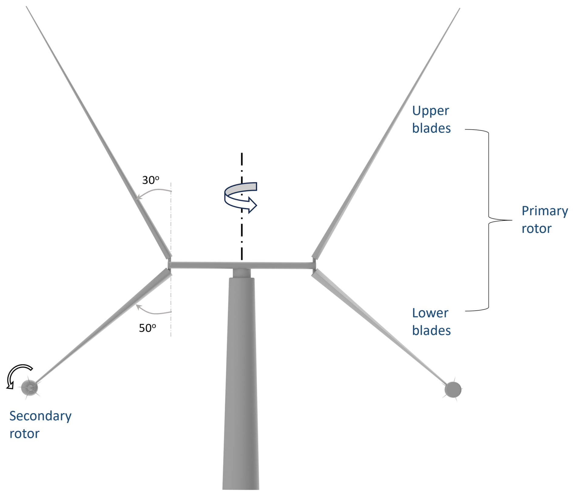
The X-Rotor geometry (Fig. 1) consists of two main components: an X-shaped VAWT (primary rotor) and two tip-mounted HAWTs (secondary rotors). The primary rotor has a distinctive “X” shape, with a set of coned upper and lower blades connected by a cross-beam that serves as a strut. The secondary rotors are attached at the lower blade tips and experience a significantly increased inflow speed due to the relative velocity at the primary rotor blade tips. The thrust of the secondary rotors determines the rotational speed of the overall turbine, and all electrical power is extracted from them. These rotors are connected to high-speed direct-drive generators instead of using gearboxes, which substantially reduce the turbine's capital expenditure (CapEx). Additionally, the low altitude and reduced mass of the generators eliminate the need for jack-up vessels for maintenance, potentially lowering operating expenses (OpEx) and maintenance expenses (Flannigan et al., 2022). The upper blades of the X-Rotor are pitch controlled and designed to shed aerodynamic power in the above-rated conditions (Recalde-Camacho et al., 2024). The lower blades are not pitch controlled, as any adjustment to them would disrupt the operation of the secondary rotors. A recent study on the operational expenditure of the X-Rotor concept by Flannigan et al. (2022) demonstrated significant savings in the CapEx and OpEx compared to an HAWT. Similarly, a feasibility study by Leithead et al. (2019) showed up to 26 % overall cost savings compared to HAWTs. Furthermore, the coned angles of the X-Rotor blade allows it to use less material per surface area compared to other traditional VAWTs, significantly reducing CapEx costs compared to VAWTs.

Figure 1 A geometric rendering of the X-Rotor with the different components.

Existing aerodynamic studies on the X-Rotor geometry are quite limited. Morgan and Leithead (2022) provided an initial characterisation of the X-Rotor using a double multiple streamtube (DMS) method. Later, Morgan et al. (2025) demonstrated the power gains achieved by coned blades compared to non-coned blades for a given blade span using a 2D actuator cylinder approach. In our earlier work, we systematically compared aerodynamic models – ranging from low-fidelity BEM models to high-fidelity blade-resolved URANS CFD models – on the power, thrust, and load characteristics of a full-scale X-Rotor at various operational blade pitch offsets (Giri Ajay et al., 2024). We concluded that low-fidelity BEM models, such as DMS and 2DAC, are unsuitable for modelling the X-Rotor across its full operating range due to vertical induction from coned blades and stronger tip vortices under pitch-offset conditions. Furthermore, by comparing with high-fidelity models, we showed that free-wake vortex models are a promising alternative, offering a relatively cost-efficient approach while capturing the effects of vertical induction. Therefore, it is essential to use models that are able to capture the 3D aerodynamics of the X-Rotor geometry to be able to predict the aerodynamic behaviour accurately. However, in all these existing studies on the X-Rotor, the models were only compared to higher-fidelity simulations in limited operational cases and could not be validated with experimental data due to the full-scale rotor size.

Free-wake vortex models have previously been experimentally validated in the near wake for HAWTs (Sant et al., 2005; Gupta and Leishman, 2006; Van Den Broek et al., 2023). Similar validations have been conducted for H-type VAWTs (Ferreira et al., 2010; Meng et al., 2014; Tescione et al., 2016), demonstrating that free-wake vortex models are highly effective in accurately capturing the VAWT's near wake.

Recently, two experimental campaigns of a 1:100 scaled X-Rotor geometry (Fig. 1) were conducted. Bensason et al. (2023) obtained phase-locked PIV data of the induction field of the rotor with no pitch offsets. The dataset consisted of planar slices at different locations inside the rotor volume to examine the influence of the coned blades on the vorticity field. Later, Bensason et al. (2024) captured additional phase-locked data in the near wake of the turbine with pitch offsets, focusing on their impact on the near-wake flow.

This study aims to validate the aerodynamic characteristics of the scaled X-Rotor predicted by CACTUS by comparing numerical simulations with wind tunnel measurements for both non-pitched and pitched cases. Furthermore, it examines the influence of the coned blades on blade loads and the flowfield as a function of rotor height. Since wake and vortex structures depend on blade loads, this study strengthens confidence in using free-wake vortex models for unconventional turbines. Additionally, it provides valuable insights into the X-Rotor's aerodynamics, supporting its future development.

2 Experimental approach

In this section, we provide a brief description of the rotor model used in the experiments and the experimental setup. Detailed information on setup and measurement techniques can be found in Bensason et al. (2023, 2024).

2.1 Scaled X-Rotor model

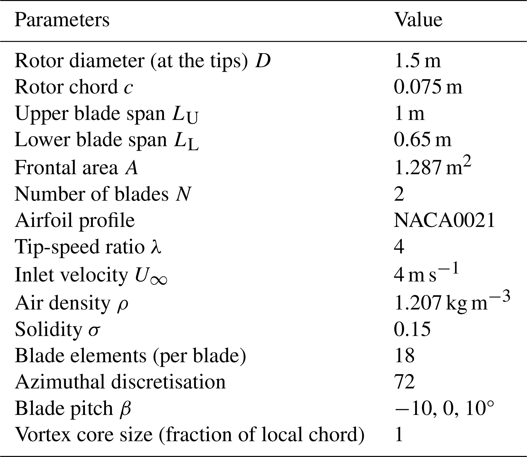
The test geometry is a purely geometrically scaled model of the full-size primary rotor, reduced by a factor of $\frac{\mathrm{1}}{\mathrm{100}}$. The top and bottom blades have a tip diameter of D=1.5 m and cone angles of 30° and 50°, respectively, resulting in upper and lower spans of 1 and 0.65 m, respectively. Aside from scaling, the primary difference between the full-scale turbine and the scaled model is that the latter consists of four straight NACA0021 airfoils with a constant chord of c=0.075 m, attached to a stiff cross-beam that has a length of 0.5 m and the same profile and chord. The blades are clean, without any vortex generators, and are mounted at $c/\mathrm{2}$. The rotor is supported by a tower with a diameter of 0.06 m. The model operates at a constant tip-speed ratio of λ=4.0 at U_∞=4 m s⁻¹, yielding a chord-based Reynolds number of $R{e}_{\mathrm{c}}=\mathrm{8.1}\times {\mathrm{10}}^{\mathrm{4}}$ at the tip. The operating conditions are determined to obtain a thrust coefficient so as to be as close as possible to the optimal value of C_T=0.7, without compromising the structural integrity of the rotor.

A visualisation of the tip trajectory is provided in Fig. 2. A constant inflow velocity of U_∞=4 m s⁻¹ is assumed, neglecting the influence of induction. Blades (B) 1 and 2 represent the blades at azimuth θ=0 and 180°, corresponding to the rotor's perpendicular position to the flow (maximum frontal area), as labelled in Fig. 2. The top (t) and bottom (b) blade pairs follow the same convention. The structures associated with each blade (B1t, B2t, B1b, B2b) are distinguished by colour. As the blades progress over time, the resulting flow structures from each blade convect downstream, eventually overlapping and interacting with others. Visualisations of each phase are provided here as a reference for analysing the flowfields at the specified streamwise locations within the volumes.

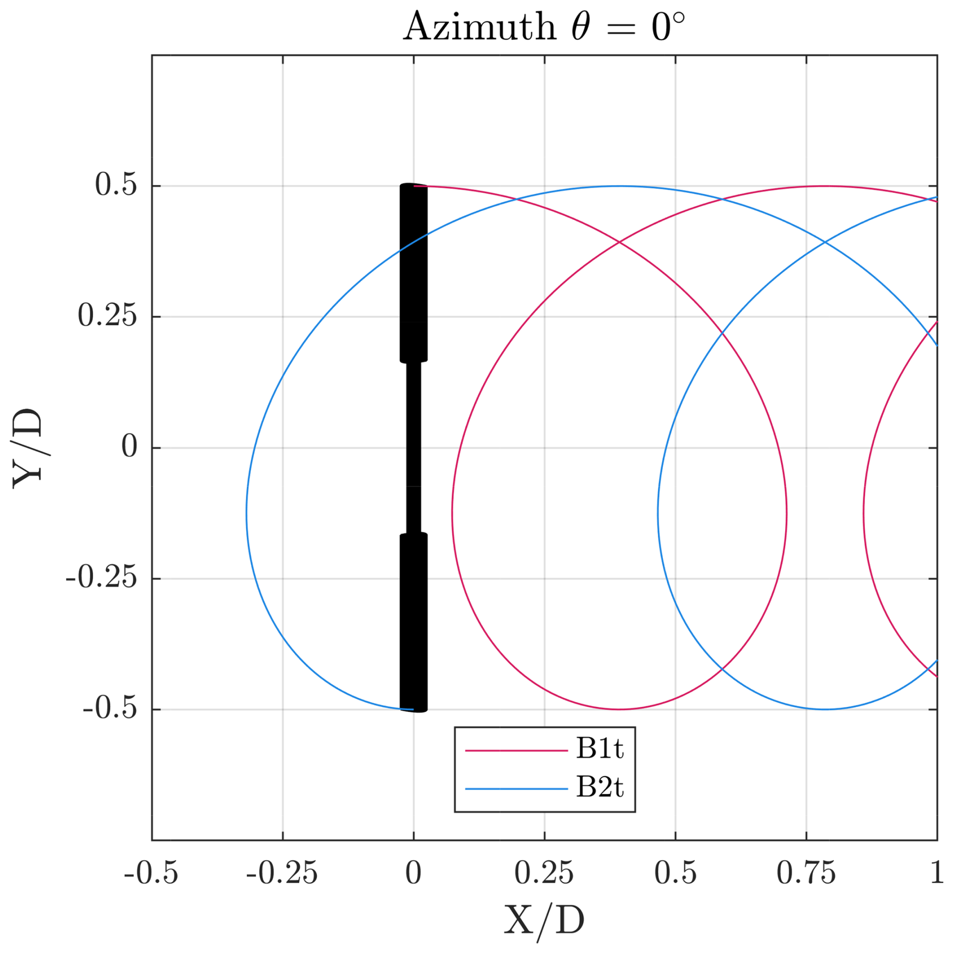
Figure 2 Top-view schematic of tip trajectory of the top blades at azimuth θ=0°. The tip trajectory is mapped to each blade, in this instance labelled B1t and B2t, for the two blades in the top half (t). Corresponding blades in the bottom half would be referred to as B1b and B2b, respectively. No wake expansion or induction is assumed.

2.2 Experimental setup

The experiments are conducted in the Open Jet Facility (OJF) at TU Delft Aerospace Engineering, as illustrated in Fig. 3. A controlled streamwise velocity of U_∞=4 m s⁻¹ is maintained throughout the experiment. The resulting inflow has reported turbulence intensities of 0.5 % within the testing region (Lignarolo et al., 2014). The measurement system captures phase-locked flowfield measurements at various locations within the X-Rotor induction field. Normalised cross-stream locations $x/D=-\mathrm{0.435},-\mathrm{0.265},-\mathrm{0.065},\mathrm{0},\mathrm{0.065},\mathrm{0.265},and\mathrm{0.435}$ were measured at azimuths $\mathit{\theta }=\mathit{\{}\mathrm{0}\mathit{°},\mathrm{45}\mathit{°},\mathrm{90}\mathit{°},\mathrm{135}\mathit{°}\mathit{\}}$. At each cross-stream location, multiple planes are recorded along the y and z axis, using a traversing system, and then stitched together. Due to time constraints, not all phase and wake locations were measured with the same level of detail, leading to variations in the number of planes recorded for each wake-phase pair. Additionally, because of the camera orientation relative to the measurement planes, frequent masking operations are applied to eliminate shadows. Given the placement of the PIV system, the measurements primarily focus on the windward half of the cycle ($Y/D>\mathrm{0}$).

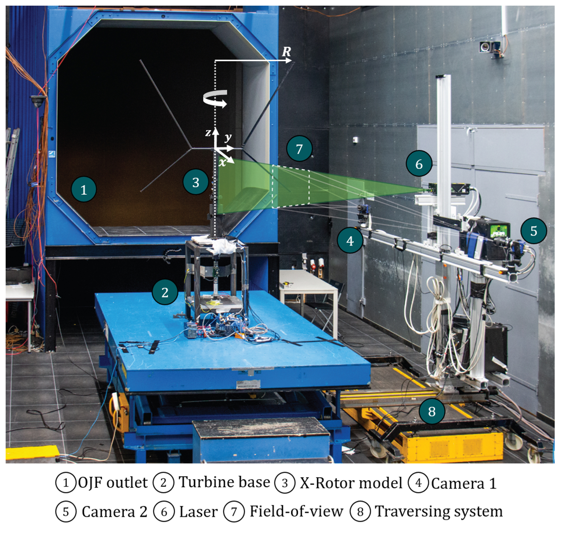
Figure 3 Experimental setup in the OJF adapted from Bensason et al. (2023). The origin of the coordinate system is placed at the centre of the cross-beam. The axis and direction of rotation are marked (anti-clockwise) with a curved arrow, and the tip radius R is marked. A visualisation of the measurement plane is provided (green cone). A similar setup for the second experimental campaign is presented in Bensason et al. (2024).

2.3 Uncertainty of the flowfield measurements

The diffraction-limited minimum image diameter is of practical significance for optical measurements such as PIV. Following Eq. (1), the smallest particle image that can be obtained using the given imaging configuration is defined by d_diff (Adrian and Westerweel, 2011).

In this case, the magnification factor is M=0.01 (sCMOS camera catalogue, 6.5 µm). The lens used has a focal length f of 106 mm, resulting in an object imaging distance (d_o) of 101 mm. The f-number f_# for this experiment is set to 8, and the sCMOS cameras have a wavelength of λ=523 nm (catalogue). Consequently, d_diff is 10.1 µm. Given a particle pixel diameter d_p of approximately 3 µm, the ratio $d_{\mathrm{diff}}/d_{\mathrm{p}}$ is 3.4.

$$\begin{array}{}\text{(1)}& d_{\mathrm{diff}}=\mathrm{2.44}\times f_{\mathit{\#}}\times (M+\mathrm{1})\times \mathit{\lambda }\end{array}$$

We can also examine the standard uncertainty in the mean flowfield. Using the approach of Sciacchitano and Wieneke (2016), the standard uncertainty is calculated using Eq. (2). For each measurement, we average over N=120 samples. The standard deviation of the velocity σ_U consists of all three velocity components and varies across the plane, both temporally and spatially. In general, regions with high vorticity (such as tip vortices and shed vorticity) exhibit a velocity standard deviation of σ_U=0.24 m s⁻¹, with the highest component occurring out of the plane, while the other two components are 0.19 and 0.15 m s⁻¹. In wake regions where no vortical structures are present, the velocity standard deviation is lower, approximately σ_U=0.05 m s⁻¹, with all components being similar in magnitude. Using the highest value for calculation, the standard uncertainty of the mean velocity is U_U=0.02 m s⁻¹, which corresponds to 0.5 % of the free-stream velocity.

$$\begin{array}{}\text{(2)}& U_{\mathrm{U}}={\displaystyle \frac{{\mathit{\sigma }}_{\mathrm{U}}}{\sqrt{N}}}\end{array}$$

A similar uncertainty analysis is conducted for cases with blade pitch offset and is presented in detail in Bensason et al. (2024).

3 Numerical setup

3.1 CACTUS free-wake vortex model

The Code for Axial and Cross-flow TUrbine Simulation (CACTUS) is an open-source vortex model tool for wind turbine simulations, developed by Murray and Barone (2011). In this approach, the blades are represented as a lifting line, with a vortex lattice system formed by the surrounding bound, shed, and trailing circulations (Fig. 4).

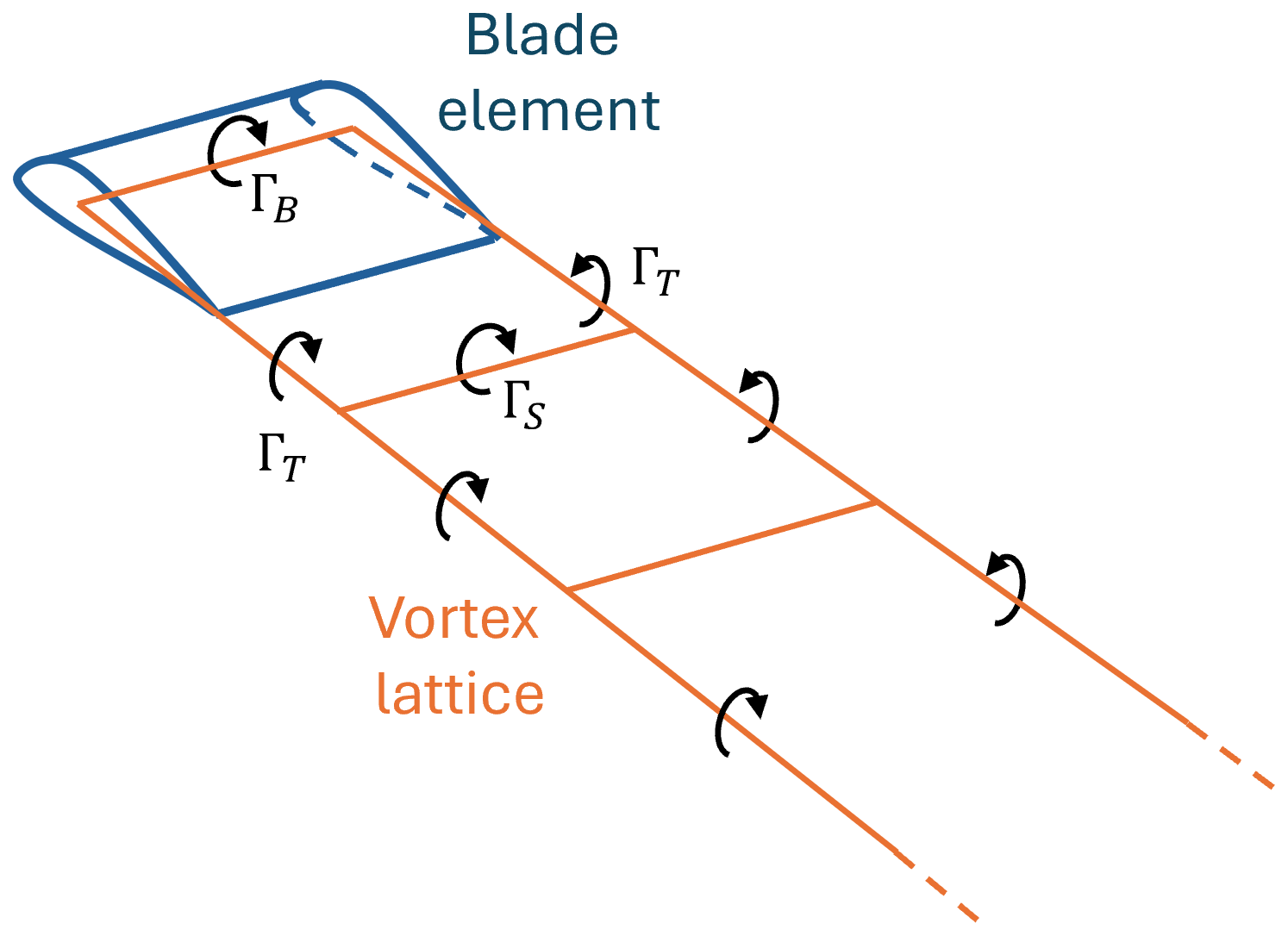
Figure 4 The vortex lattice system of a single blade element along with the bound (Γ_B), shed (Γ_S), and trailing (Γ_T) circulations.

The flowfield is constructed using this vortex lattice, where the velocity is the arithmetic sum of the freestream velocity and the velocity induced by the vortices. This is determined using the Biot–Savart law (Katz and Plotkin, 2009), which expresses the velocity field as a function of the circulation of any line segment within the vortex lattice, as follows:

$$\begin{array}{}\text{(3)}& {\mathit{u}}_a={\displaystyle \frac{\mathrm{\Gamma }}{\mathrm{4}\mathit{\pi }}}{\displaystyle \frac{{\mathit{r}}_{\mathrm{1}}\times {\mathit{r}}_{\mathrm{2}}}{|{\mathit{r}}_{\mathrm{1}}\times {\mathit{r}}_{\mathrm{2}}{|}^{\mathrm{2}}}}({\mathit{r}}_{\mathrm{1}}-{\mathit{r}}_{\mathrm{2}})\cdot \left({\displaystyle \frac{{\mathit{r}}_{\mathrm{1}}}{\left|{\mathit{r}}_{\mathrm{1}}\right|}}-{\displaystyle \frac{{\mathit{r}}_{\mathrm{2}}}{\left|{\mathit{r}}_{\mathrm{2}}\right|}}\right).\end{array}$$

Here, u_a represents the velocity vector at point a, while r₁ and r₂ are the displacement vectors from the ends of the vortex line segment to point a. The circulation of the vortex line segment is denoted by Γ.

In this study, we used CACTUS to model the scaled X-Rotor, representing each of the upper and lower blades as lifting lines. Additionally, we implement the free-wake vortex algorithm in CACTUS, which calculates the wake convection velocity at each time step. To model the circulation distribution, the NACA0021 blade airfoil profile is characterised using an airfoil polar dataset, which is further detailed in Sect. 3.2.

3.2 NACA0021 airfoil dataset and its uncertainty

In our study, the experiments operate at a chord-based Reynolds number of $Re=\mathrm{81}\times {\mathrm{10}}^{\mathrm{3}}$. Melani et al. (2019) collected experimental and numerical polars for the NACA0021 airfoil across different Reynolds number ranges: low (40–80×10³), medium (80–700×10³), and high ($\ge \mathrm{700}\times {\mathrm{10}}^{\mathrm{3}}$). In the low ranges, there is a significant deviation among the polar profiles, due to measurement uncertainties. In contrast, in the medium and high ranges, the polars exhibit much better agreement among each other. Therefore, we can understand that at these low Reynolds numbers, the polars are somewhat uncertain. Regardless, to present a very conclusive study, we generated the airfoil polars using XFOIL (Drela, 1989) at a Reynolds number of $Re=\mathrm{81}\times {\mathrm{10}}^{\mathrm{3}}$ for the X-Rotor, with an Ncrit of 4 (based on the experimental turbulence intensity). The static stall angle in this case is around α_ss=9°. The post-stall characteristics are obtained using a Viterna extrapolation technique (Viterna and Janetzke, 1982).

To elaborate on the uncertainty of the polars, Fig. 5 presents the lift coefficient C_l as a function of angle of attack α at the operational Reynolds number. In general, the polars predicted by XFOIL predict a steeper slope in the lift profile compared to the experiments. This is most clearly observed in the section before the static stall. This slope decreases with decreasing Ncrit value. However, it is very evident that there is a large discrepancy between the different polars – even among experiments. The two experiment profiles vary quite significantly due to uncertainty in measurement, corroborating the analysis of Melani et al. (2019). This highlights the challenges in achieving accurate airfoil data at these low Reynolds numbers and the importance of considering these uncertainties in aerodynamic analyses. In our study, we expect most discrepancies to be due to the uncertainty described here. We shall discuss these further in Sect. 4.

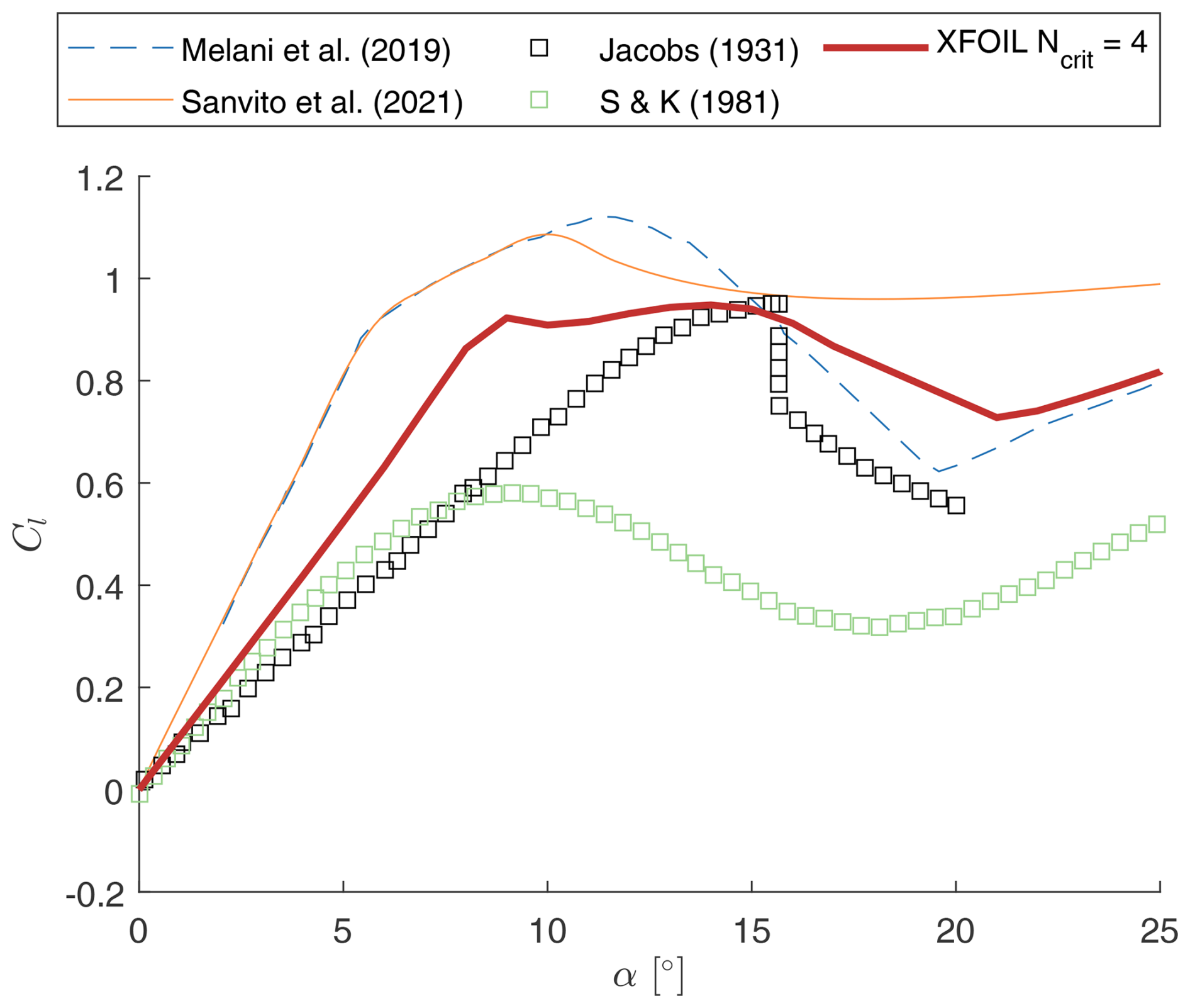
Figure 5 Comparison of lift coefficient C_l and angle of attack α for NACA0021 airfoil datasets at $Re=\mathrm{81}\times {\mathrm{10}}^{\mathrm{3}}$. Markers correspond to the experimental datasets from Jacobs (1931) (black) and Sheldahl and Klimas (1981) (green). The dashed blue line and solid orange line correspond to the XFOIL polars generated by Melani et al. (2019) and Sanvito et al. (2021). The solid red line corresponds to the XFOIL polars used in this study.

3.3 Dynamic stall and flow curvature models

Dynamic stall models are used to evaluate the unsteady effects on the lift, pitching moments, and drag of the blade sections, enabling more accurate predictions from the free-wake vortex model (Masson et al., 1998; Buchner et al., 2018; Le Fouest and Mulleners, 2022). Considering the operational Reynolds number of the scaled X-Rotor, we employ the Leishman–Beddoes (LB) dynamic stall model (Sheng et al., 2006, 2008), which is readily available in CACTUS. The LB model simulates the dynamic stall process by solving a set of first-order differential equations and utilising empirical data to represent delayed flow separation, vortex shedding, and hysteresis in lift and drag.

VAWT airfoils undergo circular motion during their azimuthal cycle, which can be decomposed into translation and pitching motion. This pitching component leads to a variation in the inflow (by extension a variation in angle of attack) along the chord of the blades, which introduces flow curvature effects that must be compensated for by an additional angle of attack or virtual camber (Migliore et al., 1980; Cardona, 1984; Rainbird et al., 2015). While this provides a more accurate depiction of airfoil motion in VAWTs, we opt not to include it here for two critical reasons. Primarily, implementing the flow curvature model (such as Goude, 2012) to a rotor geometry with a large spanwise relative velocity distribution would make it exceedingly difficult to isolate the differences observed between CACTUS and the experimental results for other factors. Moreover, geometrical virtual airfoil transformations (such as Hirsch and Mandal, 1984) show large inaccuracies at high chord-to-radius ratios ($c/R>\mathrm{0.2}$), which is the regime that most of the X-Rotor blade operates in. Second, as CACTUS does not inherently come with a flow curvature correction model, implementing it ourselves in the source code would be outside the scope of this study. Furthermore, attempting to pre-emptively correct the airfoil polars without calculating the relative velocities would result in unwarranted errors in CACTUS. We believe that the flow curvature model is essential for this geometry but would bring uncertainty to the results when the behaviour of the rotor with and without flow curvature has not been tested for this geometry. This is indeed a limitation in our approach as the lack of flow curvature would introduce differences in the blade forces and affect the near wake due to the change in vortex field. As highlighted by Goude (2012), the flow curvature model would introduce a net positive angle of attack to the blade in the upwind half, which would redistribute the loads farther upwind (Huang et al., 2023) and directly influence the wake.

3.4 Case matrix and simulation procedure

To simulate the X-Rotor, the upper and lower blades are each discretised into 18 blade sections, which is the minimum required to achieve blade element independence of power. An additional blade section is included to smooth the transition between the upper and lower blades with fixed pitch offsets. The cross-beam and tower are not modelled, as their contributions are expected to be minimal and predictable, offering little additional insight into the aerodynamics of the X-Rotor. A constant vortex core model is employed, with the vortex core set to 100 % of the chord-to-radius ratio. The simulations are run for 10 revolutions to ensure convergence, using a second-order predictor explicit time-advancement scheme. A sensitivity analysis was conducted on vortex core size, dynamic stall, and the effects of lift and drag coefficients for the airfoil. To maintain focus on the main findings, this analysis is presented separately in Appendix A. The conclusions drawn from the sensitivity study informed the final setup parameters summarised in Table 1. The solidity σ of the X-Rotor is determined using the derived expression $\mathit{\sigma }=\frac{Nc(L_{\mathrm{U}}\cos \mathrm{30}\mathit{°}+L_{\mathrm{L}}\cos \mathrm{50}\mathit{°})}{A}$, where N is the number of blades, L_U and L_L are the upper and lower blade spans, c is the chord, and A is the rotor frontal area. The angles correspond to the coned angles of the upper and lower blades.

Table 1 Description of the simulation setup for CACTUS.

4 Results

4.1 Validation study – non-pitched case

The streamwise velocity $u/U_{\mathrm{\infty }}$ and vorticity ${\mathit{\omega }}_{x}D/U_{\mathrm{\infty }}$ contours at different azimuthal positions $\mathit{\theta }=[\mathrm{0}\mathit{°},\mathrm{45}\mathit{°},\mathrm{90}\mathit{°},\mathrm{135}\mathit{°}]$ are compared between CACTUS simulations and the experimental outputs in Figs. 6 and 7, respectively. The planes are located at $X/D=-\mathrm{0.27}$, 0.067, 0.27, and 0.43 and showcase the simulations in the upper tile and the experimental results in the lower tile for each phase. The plane $X/D=\mathrm{0}$ was not measured in the experiment as it produced considerable reflection, inducing high uncertainty in the PIV processing.

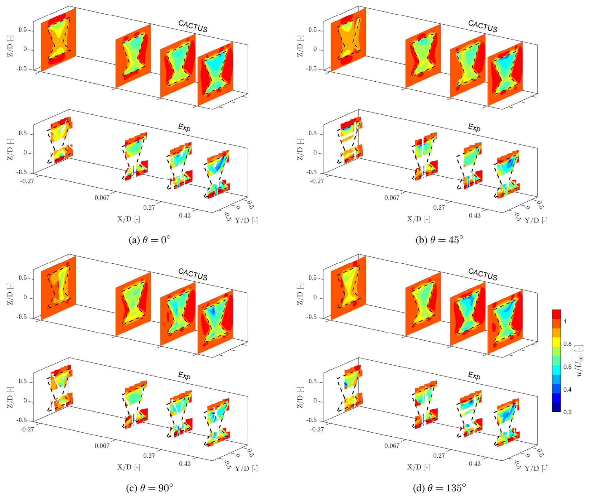
Figure 6 Normalised streamwise velocity ($u/U_{\mathrm{\infty }}$) contours of the X-Rotor at azimuths $\mathit{\theta }=[\mathrm{0}\mathit{°},\mathrm{45}\mathit{°},\mathrm{90}\mathit{°},\mathrm{135}\mathit{°}]$ at downstream locations $X/D=-\mathrm{0.27},\mathrm{0.067},\mathrm{0.27},\mathrm{0.43}$, respectively, where D is the rotor diameter for CACTUS (top) and experiments (bottom). The numerical and experimental results are shown in the upper and lower tiles, respectively. The dashed black lines indicate the projected frontal area of the rotor on the corresponding plane. The x axis is magnified to enhance visibility.

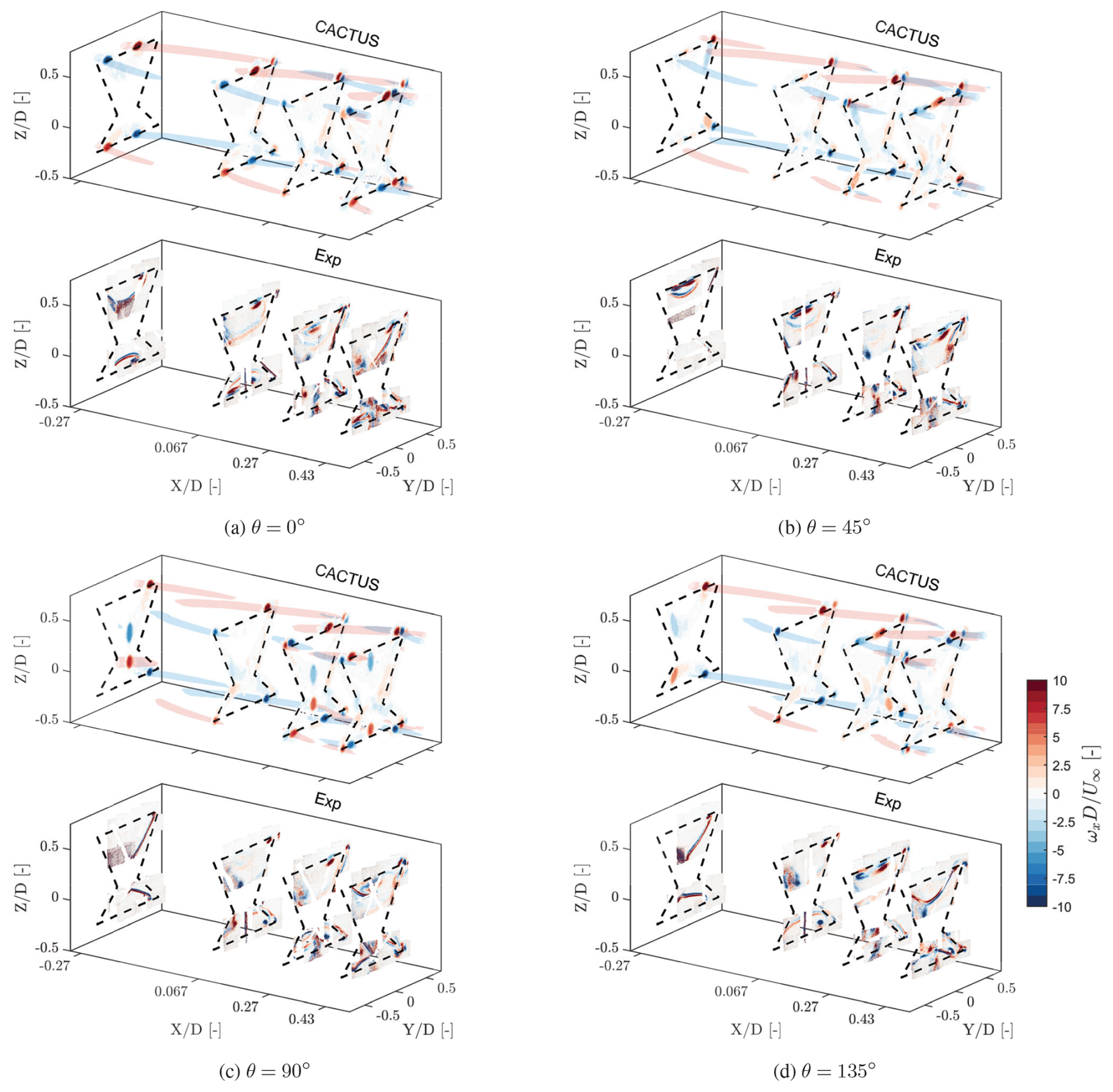
Figure 7 Normalised streamwise vorticity (${\mathit{\omega }}_{x}D/U_{\mathrm{\infty }}$) contours of the X-Rotor at azimuths $\mathit{\theta }=[\mathrm{0}\mathit{°},\mathrm{45}\mathit{°},\mathrm{90}\mathit{°},\mathrm{135}\mathit{°}]$ at $X/D$ = –0.27, 0.067, 0.27, 0.43, respectively, where D is the rotor diameter for CACTUS (top) and experiments (bottom). CACTUS isosurfaces are overlayed to show the evolution of the vortices with a non-dimensionalised strength of 6 and above. The dashed black lines indicate the projected frontal area of the rotor. Very low values of vorticity are hidden, and the x axis is magnified to enhance visibility.

Overall, the velocity predictions within the rotor volume show good agreement with the experimental results, as observed in Fig. 6, except for the wake of the tower, which is not modelled in CACTUS. The flowfield trends align well with experimental data, with velocity deficits accurately represented in the regions of blade passage across all azimuths. The induction in the upwind plane at $X/D=\mathrm{0.27}$ is also well predicted. Some minor discrepancies are expected, as CACTUS does not account for blade deflection and deformation caused by centrifugal forces and the high rotational speed of the rotor. This is particularly noticeable at the windward tips ($Y/D>\mathrm{0}$), where the experimental results show velocity deficits extending beyond the projected frontal area of the rotor – an effect not captured in CACTUS. At $X/D=\mathrm{0.43}$, CACTUS slightly underpredicts the velocity deficit across all azimuths. This difference is likely due to the challenge of uncertainty with the polars, as discussed in Sect. 3.2. If the polars were closer to the true experimental airfoil behaviour, the difference could be minimised. This holds true for the rest of the results discussed in this study.

A similar trend is observed in the vortex structures (Fig. 7), with the simulation results generally aligning well with the experiments. The elliptical vortical structures seen in the experiments correspond to the shed vortices from the blades, as detailed in Bensason et al. (2023). These vortices take on an elliptical shape due to the coned geometry of the X-Rotor blades. While the shed vortices are captured in the CACTUS model, they appear as faint smears (e.g. in the upper half at θ=0° and $X/D=\mathrm{0.067}$) and are significantly weaker in magnitude compared to the experimental results. This discrepancy is once again attributed to the airfoil polar uncertainty. The isosurfaces further illustrate the evolution of dominant vortices in the CACTUS simulations. Comparing with Fig. 2, the vortices generated at $X/D=-\mathrm{0.27}$ at θ=0° originate from the passage of B2t and B2b. At $X/D=\mathrm{0.067}$, these vortices intersect the windward tip, while the other dominant vortices are remnants from the previous cycle of B1t and B1b – evident from the isosurfaces, which reveal two sets of trailing vortices convecting downstream. This pattern extends to other planes and phases, highlighting vortex interactions between the blade passages of B1 and B2. At $X/D=\mathrm{0.43}$, the downwind passage of B1t and B1b generates three pairs of tip vortices in both the upper and lower halves of the rotor. This matches the experimental observations, although the absence of leeward planes in the measurements makes it challenging to confirm the presence of these vortex pairs definitively. Additionally, in the experiments, vortices tend to intersect the measurement plane at laterally farther locations than predicted by the simulations (e.g. tip vortices of B2t and B1t at $X/D=\mathrm{0.067}$ and $X/D=\mathrm{0.43}$). This discrepancy arises from blade deflection, which is not accounted for in CACTUS. As the blade tips deflect outward, the vortices are shed from a more laterally displaced position, affecting their subsequent convection paths.

Quantitative comparisons between the CACTUS model and the experimental results can be made by examining streamwise velocity profiles at various streamwise locations, both upstream and downstream of the rotor, across different azimuthal phases. Figure 8 presents these comparisons, showing streamwise velocity slices $u/U_{\mathrm{\infty }}$ as a function of X-Rotor height, evaluated at $Y/D=-\mathrm{0.125}$ and $Y/D=\mathrm{0.25}$ for azimuthal positions $\mathit{\theta }=[\mathrm{0}\mathit{°},\mathrm{45}\mathit{°},\mathrm{90}\mathit{°},\mathrm{135}\mathit{°}]$.

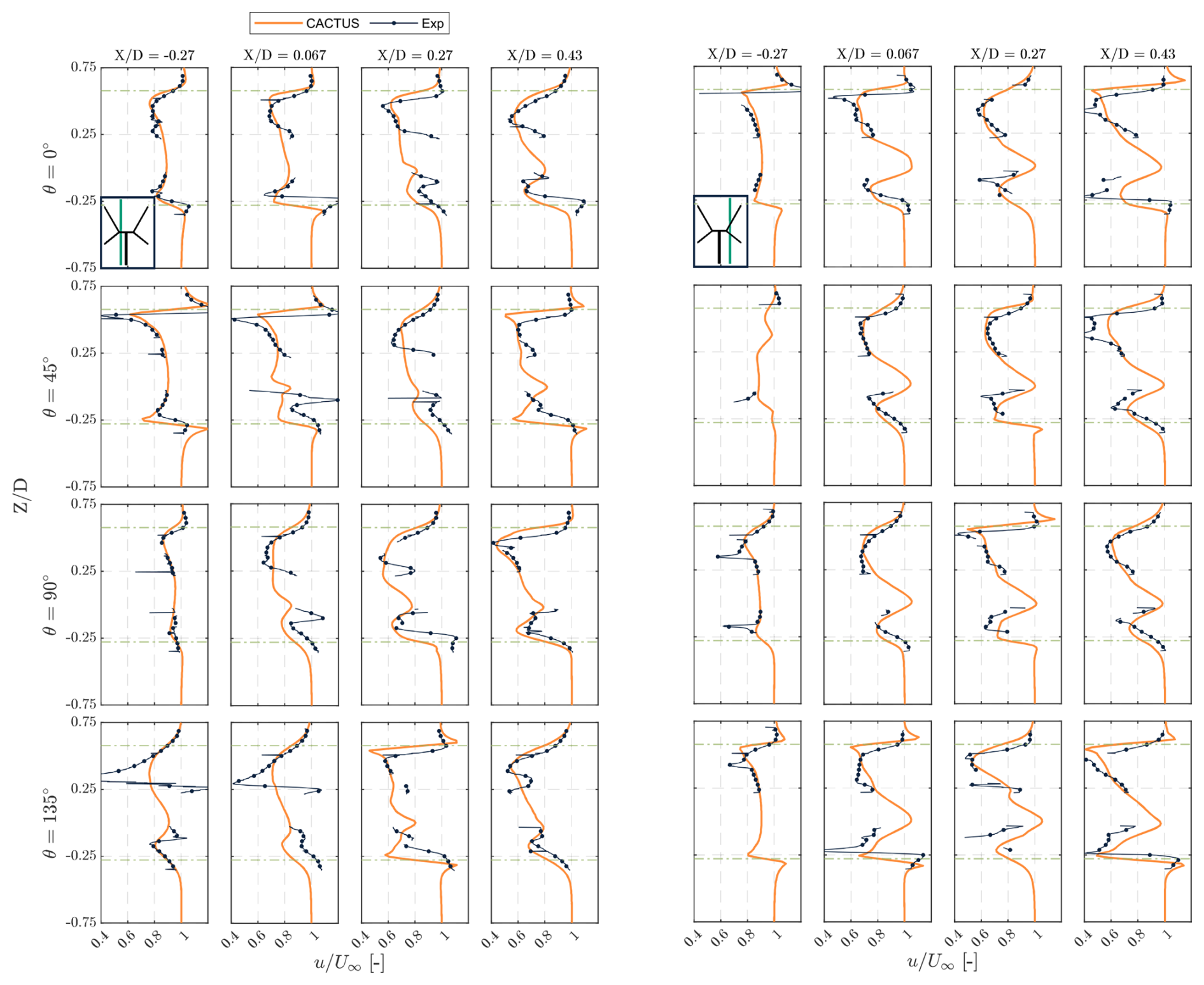
Figure 8 Comparison of the streamwise velocity $u/U_{\mathrm{\infty }}$ slices along the height of the X-Rotor at lateral position $Y/D=-\mathrm{0.125}$ (left) and 0.25 (right) at discrete streamwise locations $X/D$ = [–0.27, 0.067, 0.27, 0.43] at phase-locked azimuths $\mathit{\theta }=[\mathrm{0}\mathit{°},\mathrm{45}\mathit{°},\mathrm{90}\mathit{°},\mathrm{135}\mathit{°}]$. The inset figure in the first tile is presented to indicate the location of the slice with respect to the rotor; the green line is the $Y/D$ slice along the height of the rotor.

As expected from the earlier contour comparisons, the CACTUS results align well with the experimental data. In the leeward slice ($Y/D=-\mathrm{0.125}$), CACTUS consistently underpredicts the velocity in the lower half of the turbine, except in the most upwind plane. This discrepancy is attributed to the influence of the tower. In the experiments, the counter-clockwise rotation of the tower induces local flow acceleration on the leeward side, which is not accounted for in the CACTUS model. Since this region is close to the tower, its influence is more pronounced here than on the windward side. Additionally, CACTUS does not fully capture some of the velocity spikes observed in the experiments, particularly at θ=45° and θ=135°. This discrepancy arises from two factors: blade deflection in the experiments and the velocity field resolution in CACTUS. The former affects the vortex proximity to the measurement plane – the blade deflection in the experiments can bring vortices closer than simulated, as seen at θ=135°. The latter relates to the resolution of the volumetric velocity field obtained from CACTUS. Increasing the resolution to match the PIV planes would better capture these spikes but would also result in excessively large data files due to CACTUS's volumetric outputs. Another notable difference is the influence of the struts in the PIV data, which is evident at θ=45° and $X/D=\mathrm{0.067}$. In the windward slice ($Y/D=\mathrm{0.25}$), the differences between CACTUS and the experiments are lesser than the leeward side. The influence of the tower is minimised as there is no observable trend of overprediction or underprediction from CACTUS in the lower half of the rotor. The upwind plane has the best match, while the differences increase as we move downwind. At θ=135°, the planes $X/D=\mathrm{0.067}$ and 0.27 have the most observable deviations. This is due to the blade–wake interaction occurring at this azimuth, which is underrepresented in CACTUS compared to the experiment. As with the leeward side, the peaks of velocity profiles occur at different heights due to the deflection of the blade not being modelled in CACTUS. Once again, the ability to resolve the spikes is largely dependent on the resolution of the velocity field obtained from CACTUS (notably seen at $X/D=\mathrm{0.43}$ for θ=0°). Overall, the trends of the wake are captured and the velocity deficits are predicted well, which indicates that CACTUS can be a good tool to represent the velocities inside the volume of the X-Rotor.

4.2 Validation study – pitched case

Similar to the work by Bensason et al. (2024), a positive pitch corresponds to orienting the leading edge towards the rotation axis, while a negative pitch directs it away. Additionally, in line with the original control strategy of the X-Rotor design (Leithead et al., 2019), the lower blades are not pitched along with the upper blades. The experiments measured the planes downwind of the rotor for all three pitch cases, $\mathit{\beta }=-\mathrm{10}\mathit{°},\mathrm{0}\mathit{°}$ (baseline), and 10°, at an azimuth of θ=0° but only for the upper blades.

To facilitate comparison, Figs. 9 and 10 present the normalised streamwise velocity $u/U_{\mathrm{\infty }}$ and vorticity ${\mathit{\omega }}_{x}D/U_{\mathrm{\infty }}$ for the three pitch cases in both CACTUS simulations and experimental results.

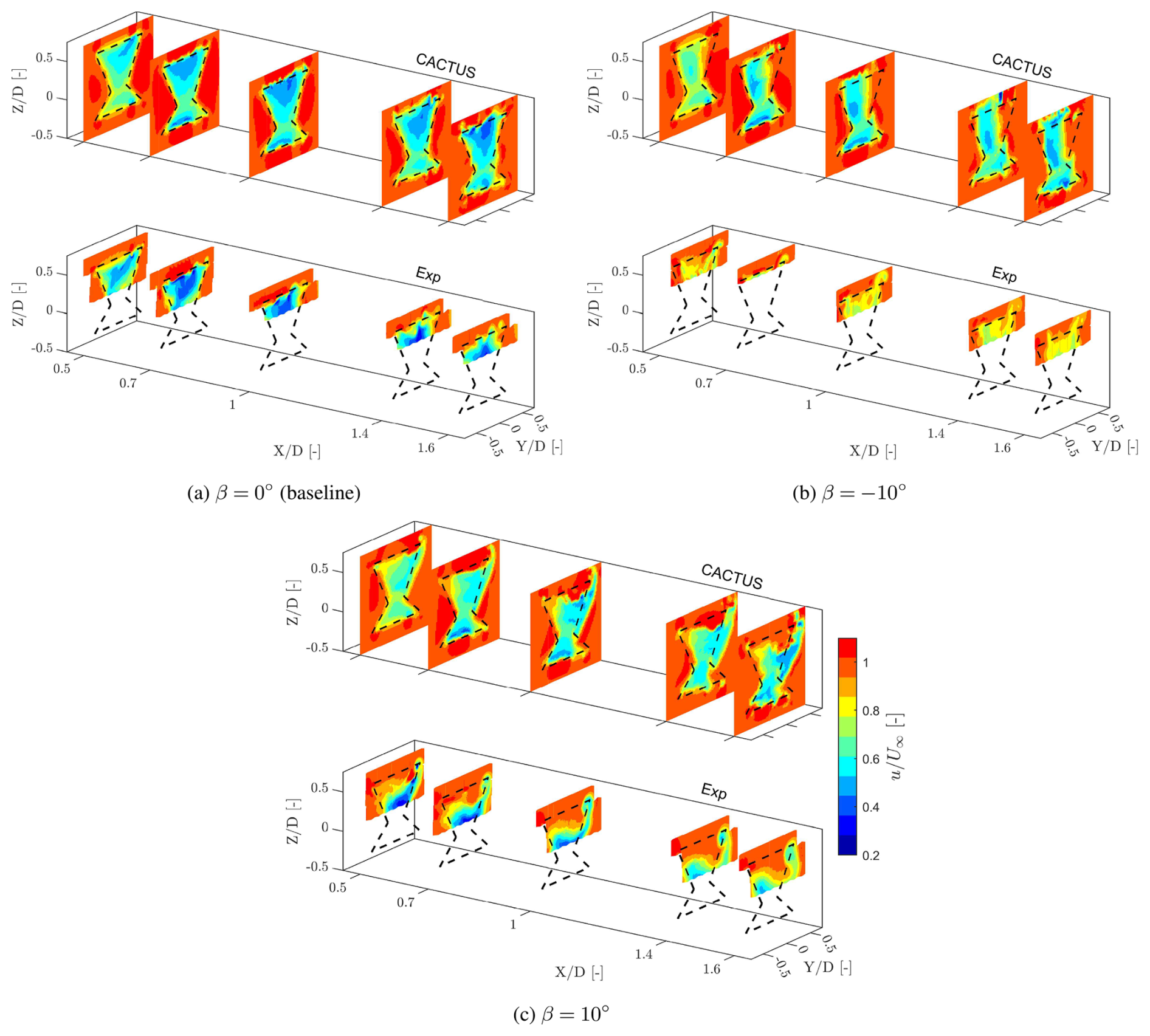
Figure 9 Normalised streamwise velocity ($u/U_{\mathrm{\infty }}$) contours of the X-Rotor with pitch offset β = 0°, –10°, 10°, respectively, at downstream locations $X/D=\mathrm{0.5},\mathrm{0.7},\mathrm{1},\mathrm{1.4}$, and 1.6 of CACTUS (above) and experiments (below). The dashed black lines indicate the projected frontal area of the rotor on the corresponding plane. The x axis is magnified to enhance visibility.

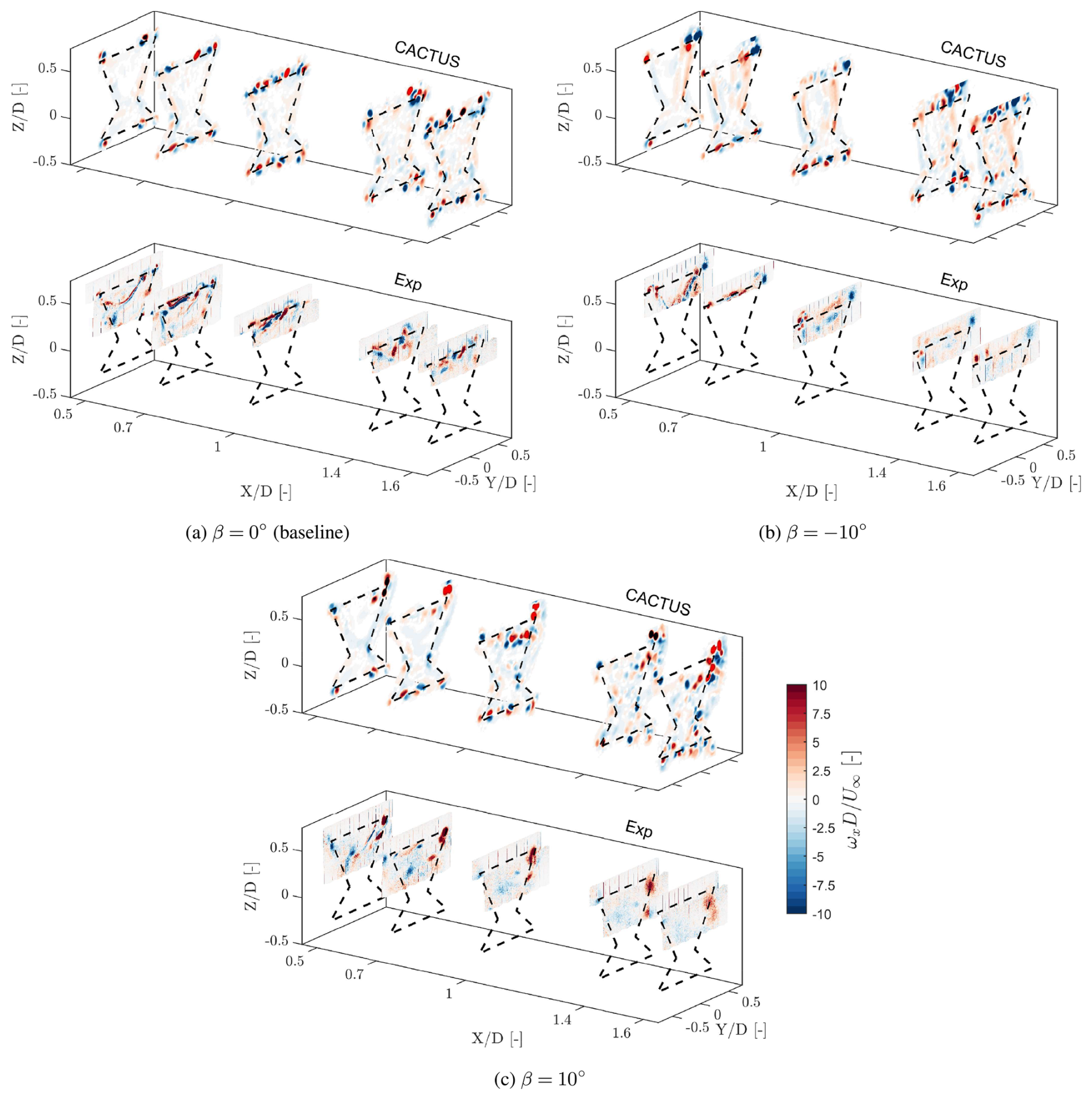
Figure 10 Normalised streamwise vorticity (${\mathit{\omega }}_{x}D/U_{\mathrm{\infty }}$) contours of the X-Rotor with pitch β = –10°, 0°, 10°, respectively, at $X/D=\mathrm{0.5},\mathrm{0.7},\mathrm{1},\mathrm{1.4}$, and 1.6 of CACTUS (above) and experiments (below). The dashed black lines indicate the projected frontal area of the rotor. The x axis is magnified to enhance visibility.

The baseline pitch case effectively extends the analysis from Fig. 6 and the discussion in Sect. 4.1. While the CACTUS model continues to capture the overall trends of the velocity profiles, it underpredicts the velocity deficit at $X/D=\mathrm{1.4}$ and beyond. The experimental results indicate that the wake centre is lower than predicted in CACTUS, although quantifying this displacement is challenging due to the limited number of measured heights in the experiments. The vortical structures observed in each plane are generally similar between CACTUS and the experiments, except for the shed vortex, which is visible at $X/D=\mathrm{0.5}$ in the experiments but not in CACTUS. Farther downstream, the vortical structures primarily consist of trailing vortices from the upper and lower blade tips. However, CACTUS appears to overpredict the vortex strengths, consistent with the discussion in Sect. 4.1. This discrepancy arises because, in the experimental results, the vortices exhibit dissipation, whereas in CACTUS, vortices generated in previous cycles remain dominant in the flow.

When pitched to $\mathit{\beta }=-\mathrm{10}\mathit{°}$, the lateral thrust of the rotor increases in magnitude, inducing a laterally inward flow into the wake (Huang et al., 2023; Giri Ajay and Simao Ferreira, 2024). This results in wake inflow from the sides and vertical outflow, a pattern observed in both the experiments and CACTUS. However, differences arise in the velocity magnitudes and wake shape. CACTUS predicts stronger lateral flow on the windward side compared to the experiment, causing the wake to contract more rapidly in this region. Additionally, CACTUS shows the wake starting to exit the top of the rotor area at $X/D=\mathrm{0.7}$, whereas this behaviour is not yet observed in the experiments. The discrepancy increases farther downstream, attributed to the stronger tip vortices predicted by CACTUS, which accelerate wake recovery compared to the experiments. Moreover, CACTUS predicts higher velocity deficits, suggesting a greater streamwise thrust than observed in the experiments. The large pitch angles in this configuration cause the turbine to operate at extreme angles of attack, well beyond stall, which significantly influences CACTUS predictions since it relies on polar data for load estimation. Bensason et al. (2024) documented substantial unsteady flow separation and turbulence on the windward side at this pitch setting, explaining the stronger windward tip vortex in CACTUS that leads to a more contracted wake. Additionally, the difference in circulation between the upper and lower blades results in a root vortex predicted by CACTUS. This vortex is visible in the windward root section and gradually moves upward downstream. Furthermore, CACTUS vortices do not dissipate as quickly as those in the experiments, further contributing to the observed differences.

In the β=10° case, the opposite wake behaviour is observed – laterally exiting through the upper half of the rotor area while freestream air enters vertically from above. The experiments indicate significant wake deflection starting at $X/D=\mathrm{0.5}$, which is greater than the values predicted by CACTUS. Additionally, CACTUS underpredicts the velocity deficit within the rotor compared to the experiments until $X/D=\mathrm{1}$, beyond which most of the experimental wake exits the captured field of view. These discrepancies are primarily attributed to the vorticity distribution arising from the load distribution. In the experiments, a dominant windward tip vortex facilitates freestream inflow from above. Meanwhile, the weaker vortices dissipate quickly, preventing them from significantly influencing the wake. In contrast, CACTUS, lacking viscous dissipation, produces numerous vortices near the windward tip, which intensify farther downstream. This incorrect vortex representation leads to inaccurate velocity predictions, preventing CACTUS from capturing the downward movement of the wake. Interestingly, the wake in the lower half of the X-Rotor shifts laterally in the opposite direction to the upper half. This is due to the formation of a root vortex that induces lateral forcing on the lower half. Once again, differences in vortex dissipation contribute to this effect – while the experimental data show a dominant tip vortex influencing vertical freestream influx, CACTUS instead predicts an accumulation of vortices near the upper half, altering the wake dynamics.

A quantitative analysis of the streamwise velocity profiles along the height of the X-Rotor is presented in Fig. 11. To ensure consistency, we selected the same lateral locations as in the discussion in Sect. 4.1.

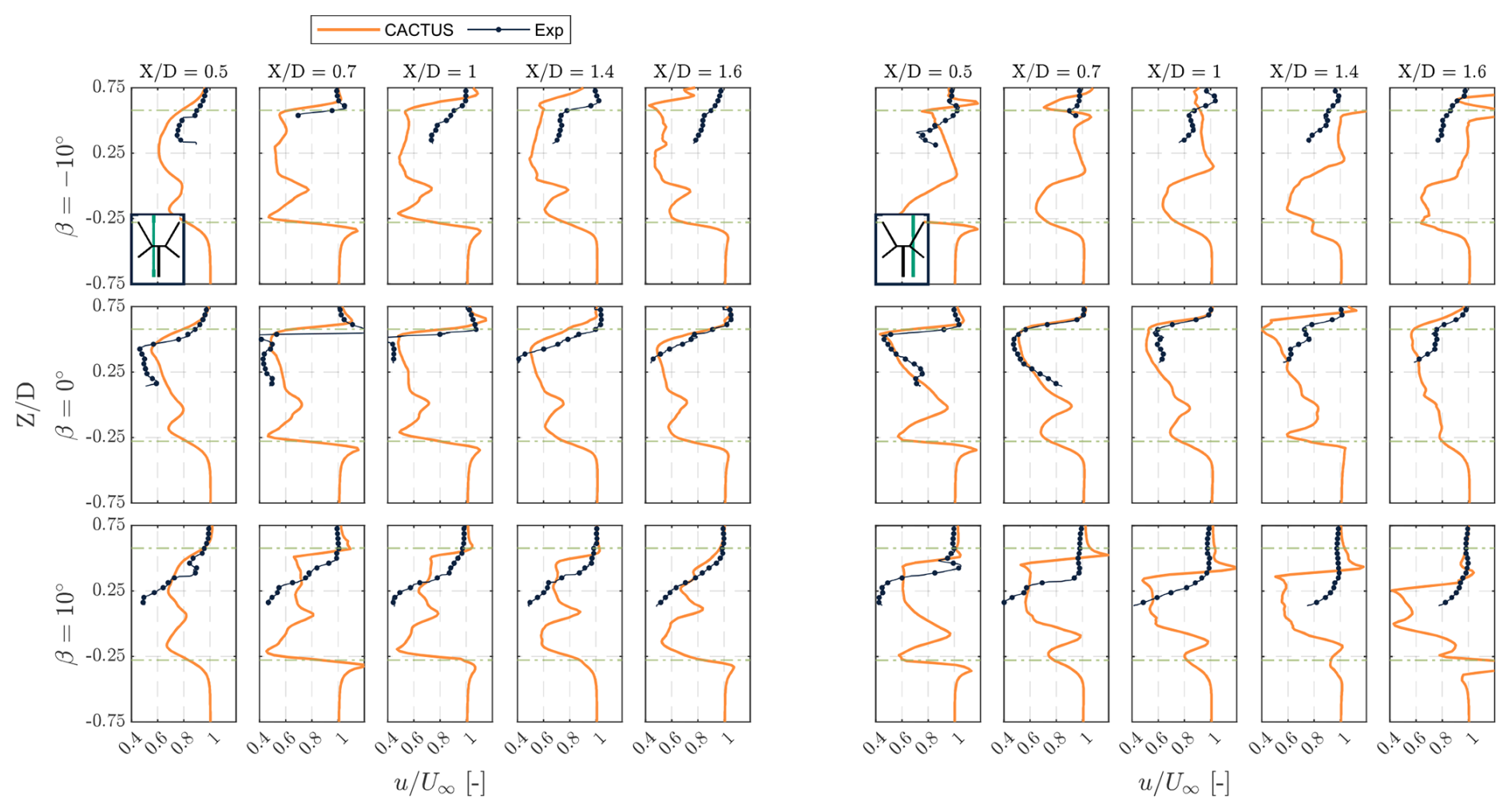
Figure 11 Comparison of the streamwise velocity $u/U_{\mathrm{\infty }}$ slices along the height of the X-Rotor at lateral position $Y/D=-\mathrm{0.125}$ (left) and 0.25 (right) at discrete streamwise locations $X/D=[\mathrm{0.5},\mathrm{0.7},\mathrm{1},\mathrm{1.4},\mathrm{1.6}]$ at pitch offsets $\mathit{\beta }=[-\mathrm{10}\mathit{°},\mathrm{0}\mathit{°},\mathrm{10}\mathit{°}]$. The inset figure in the first tile is presented to indicate the location of the slice with respect to the rotor – the green line is the $Y/D$ slice along the height of the rotor.

In the leeward slice, the velocity profile from the experiment in the baseline case is generally well represented by CACTUS, except at $X/D=\mathrm{1.4}$ and beyond, where discrepancies become more pronounced. This aligns with the earlier observation that CACTUS predicts the wake centre to be positioned higher than in the experimental results. For $\mathit{\beta }=-\mathrm{10}\mathit{°}$, a significant difference emerges between the predicted and measured values, with the experiments showing much higher velocities than CACTUS. This discrepancy increases farther downstream, reaching up to 50 % along the height. The primary cause of this difference is the previously discussed overprediction of tip vortex strength in CACTUS. At β=10°, CACTUS predictions also deviate from experimental values. While the velocity profile aligns with the experiment over a small height range in certain planes ($X/D=\mathrm{1}$ and 1.6), larger deviations occur near the root. This discrepancy is primarily due to the stronger leeward vortex predicted by CACTUS compared to the weaker vortex observed in the experiments. However, the differences in this pitch case at the leeward slice are generally smaller than those seen in the $\mathit{\beta }=-\mathrm{10}\mathit{°}$ case.

A similar pattern is observed in the windward slice – while the streamwise velocity profile is predicted relatively accurately in the baseline case, the pitched cases exhibit significant inconsistencies with the experimental profiles. These discrepancies are primarily attributed to differences in vortex strength predicted by CACTUS, which depend on the airfoil polars selected for the simulation. CACTUS struggles to accurately capture the increase in circulation induced by pitch offsets, as its predictions rely heavily on the input polars. Given that the static stall angle for these polars is α_ss=9.1°, pitching the airfoils by β=10° effectively shifts the C_l vs α profile, such that the blade would mostly operate in deep-stall conditions throughout its azimuth. As the accuracy of XFOIL becomes questionable at deep-stall conditions (Sect. 3.2), the errors are compounded. Additionally, flow curvature effects could potentially mitigate these differences by improving the vortex representation in the pitched cases, but their influence on a coned blade remains unclear. Since the wake characteristics are directly linked to blade forces, a comparison of the predicted and experimental blade loads would provide further insight. However, blade load data are unavailable for this dataset.

Overall, CACTUS appears less effective in capturing the near-wake flowfield of the X-Rotor without pitch offsets. However, the general trends and behaviour of the wake profiles predicted by CACTUS remain valuable for future research.

4.3 Influence of cone angle on the velocity field

As the CACTUS model represents the flowfield of the case without pitch offsets well, we can consider its predictions on the flowfield to be valid.

In our previous work (Giri Ajay et al., 2024), we introduced the concept of vertical induction generated by the coned blades of the X-Rotor, both with and without pitch offsets. In this section, we extend that discussion by presenting the spanwise normal force distribution and spanwise angle of attack distribution as a function of azimuth in Fig. 12. Additionally, we provide the blade-integrated forces to offer insight into the overall load contribution of the rotor. In both figures, we focus on B1 alone, rather than the entire rotor, to facilitate a more detailed discussion of the downwind half of the rotation.

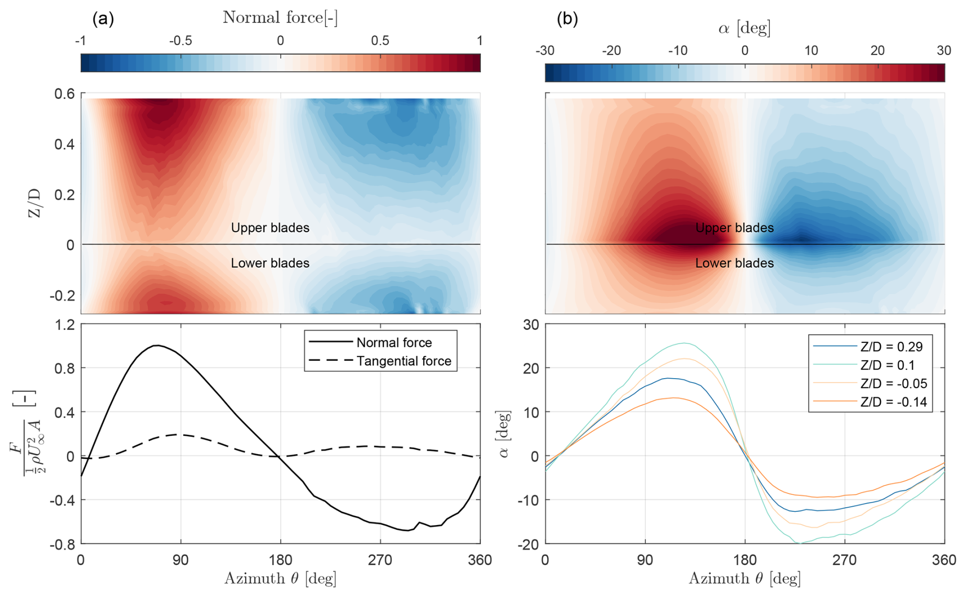
Figure 12 (a) Spanwise distribution of normal blade force as a function of height $Z/D$ and azimuth θ in the top tile and blade-integrated normal and tangential force as a function of azimuth in the bottom tile. Positive normal force is away from the axis of rotation and vice versa. Forces are integrated along both upper and lower halves of B1. (b) Angle of attack α variation along height and θ in the top tile and the bottom tile shows α at discrete locations along height.

In general, the forces in the upwind half are larger than in the downwind half, reaching their maximum near the most upwind and downwind positions. This behaviour is consistent with existing VAWT normal force profiles for non-pitched blades and aligns with our previous findings. The spanwise distribution reveals that forces are highest near the tip and lowest near the root section, which is expected as the local inflow velocity decreases closer to the root. However, some artefacts at the upper and lower tips indicate a local increase in load. Lifting-line methods consider induction only along a line at the centre of pressure (quarter chord in this case), neglecting chordwise distribution effects. This often results in an overestimation of loading near the tip (Sørensen et al., 2016). As CACTUS does not currently incorporate a correction model for this issue, and implementing one is beyond the scope of this study, we neglect this local spike as it is not critical to our analysis. Consequently, the peak load along the span occurs around $Z/D=\mathrm{0.5}$ in the upper half and $Z/D=-\mathrm{0.23}$ in the lower half, with a gradual reduction in magnitude towards the tips – an expected characteristic of a finite blade span representation in CACTUS. Interestingly, in the downwind half between θ = 270° and 330°, the forces fluctuate near the tips while remaining relatively stable elsewhere. This is attributed to blade–vortex interactions, where the blades pass through tip vortices shed during the previous cycle. This interaction is also evident in the integrated forces, where a small spike is observed in the same azimuthal range. Our previous study (Giri Ajay et al., 2024), using both another free-wake vortex model and a blade-resolved URANS approach, predicted a similar phenomenon. Since the vortices exhibit minimal vertical convection, the rest of the downwind region remains largely unaffected by blade–vortex interactions, a consequence of the coned blade geometry.

The angles of attack α decrease from the root towards the tips, reflecting the variation in local blade section rotational velocity along the height. Given that the static stall angle is α_ss=9.1°, most of the blade operates in either post-stall or deep-stall conditions between θ = 90° and 180°. The blade sections near the root ($Z/D=\mathrm{0.1}$ and $Z/D=-\mathrm{0.05}$) experience deep-stall conditions, with peak α reaching approximately 25° in the upwind half and 19° in the downwind half. This aligns with the observed low normal forces at these blade sections.

To understand the implications of the spanwise variation of normal forces on the flowfield, we present the time-averaged vertical component of velocity $\overline{w}/U$ at different height sections as viewed from above in Fig. 13.

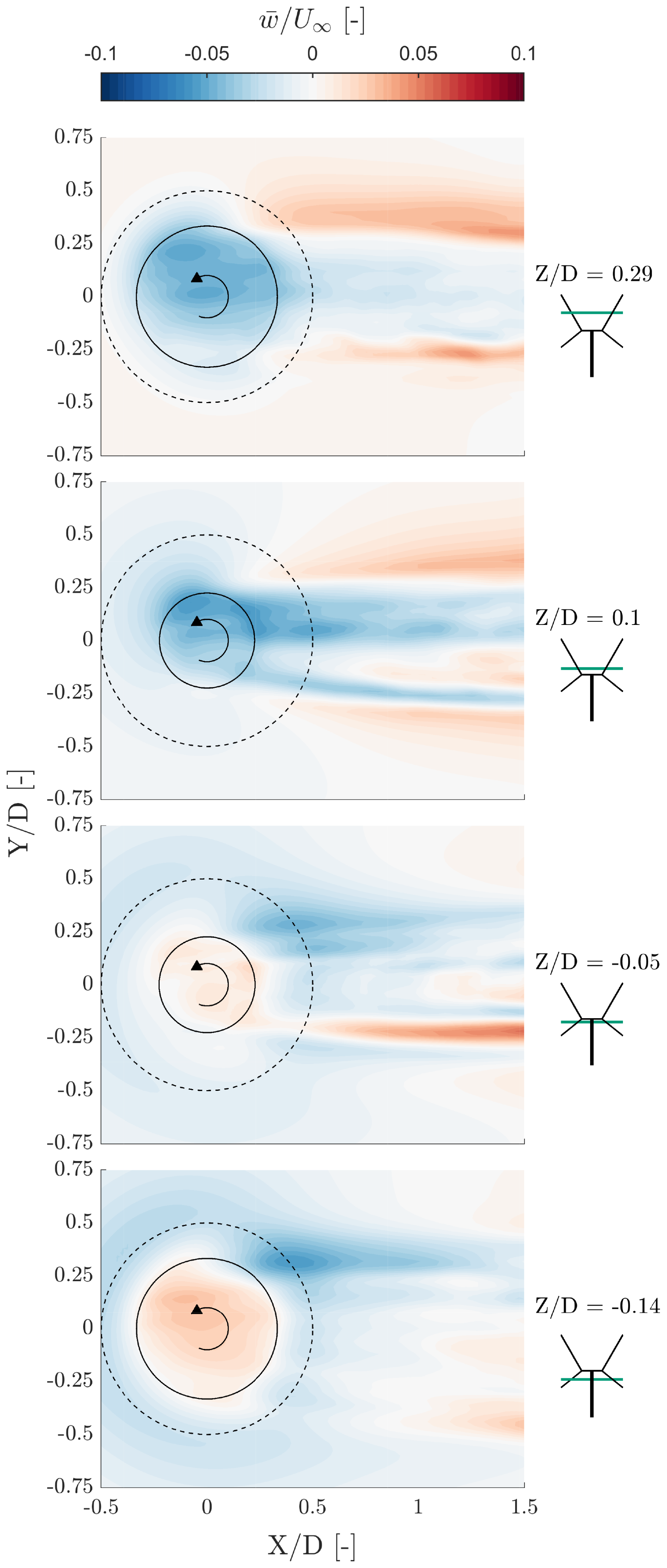
Figure 13 Time-averaged vertical component of the velocity field of the rotor at sections along the height of the rotor at $Z/D=\mathrm{0.29},\mathrm{0.1},-\mathrm{0.05}$, and −0.14, as viewed from the top. The inset figure shows the locations of the planes along the height of the X-Rotor graphically. The dashed black line indicates the tip diameter of the X-Rotor and the solid black line indicates the local diameter corresponding to the height. Red indicates upwash (out of the plane), and blue indicates downwash (into the plane).

At $Z/D=\mathrm{0.29}$, we primarily observe downwash within the rotor volume, driven by the vertical component of the normal forces from the upper blades. Interestingly, downstream of the rotor, downwash persists within the region bounded by the local diameter, whereas upwash dominates outside this region ($Z/D>\left|\mathrm{0.2}\right|$). Moreover, this upwash is stronger on the windward side than on the leeward side, indicating the influence of the tip vortices. The windward tip vortex, over a full cycle, is stronger than the leeward tip vortex. This behaviour closely aligns with the observations of Bensason et al. (2024), who reported a similar wake structure. Specifically, at β=0° in their study, the windward tip vortex induced upwash in the windward side at this plane.

At $Z/D=\mathrm{0.1}$, the downwash is stronger than at the plane above and extends farther into the wake. This is due to the cumulative contribution of downwash from the blade sections positioned above this plane. As a result, the downwash reaches farther downstream while remaining laterally confined within the bounds of the local diameter. The influence of the upper tip vortices is reduced at this plane, as it is farther from the tips, which is evident from the lower intensity of the red regions.

In the lower half of the rotor at $Z/D=-\mathrm{0.05}$, the region within the local diameter exhibits minimal upwash. This is because the downwash generated by the upper half counteracts the effect of the higher cone angle in the lower half, which results from the greater loads produced by the upper blades. Additionally, this plane captures the cumulative upwash generated by the entire lower half. However, the wake predominantly features a strong downwash – likely an effect of the lower tip vortex – but this influence does not extend significantly beyond $X/D=\mathrm{1}$. Around $Y/D=-\mathrm{0.25}$, we observe a region of upwash that extends from $X/D=\mathrm{0.5}$ to 1.5. This is due to the cumulative effect of the shed vortices from both the upper and lower blades in the leeward region, as observed from the angle of attack plots. Near the root, these shed vortices induce a resultant upwash due to the difference in cone angles between the upper and lower blades.

Finally, at $Z/D=-\mathrm{0.14}$, the region inside the local diameter is primarily characterised by upwash. However, as observed in the previous plane, the wake remains dominated by downwash. Once again, the windward side experiences stronger downwash than the leeward side, attributed to the windward tip vortex. Since the vortices shed by the lower blades rotate in the opposite direction to those from the upper blades, this behaviour is expected. Additionally, the small region of upwash in the wake is likely caused by the leeward tip vortex.

Overall, the cone angle significantly influences the flowfield, both inside and outside the rotor, and this effect is further amplified by the interaction of tip vortices when the blades are pitched.

5 Conclusions

We conducted a validation study of CACTUS, a free-wake vortex tool, against wind tunnel PIV measurements for a scaled X-Rotor VAWT, considering cases with and without blade pitch offsets. Additionally, we examined the influence of coned blades on the near wake in the absence of pitch offsets, highlighting the significance of vertical induction for such VAWT geometries. The results from CACTUS were compared with phase-locked stereo PIV measurements taken at different azimuths.

Our findings indicate that CACTUS effectively represents the flowfield within the X-Rotor volume and in the very near wake for cases without blade pitch offsets. The model captures the trends and flow features well, although discrepancies in velocity magnitude arise due to the choice of model setup parameters. The discrepancies are primarily attributed to the uncertainty in the airfoil data at the operational Reynolds number. Further inaccuracies stem from aeroelastic effects present in the experiments.

The spanwise distribution of blade forces shows a reduction in magnitude towards the root, as expected, due to the decrease in local inflow. Since the forces are more pronounced near the tips, it is evident that the coned blades significantly influence the flowfield by inducing vertical velocity.

Examining the effect of cone angle on the downstream flow, we found that a local downwash is generated within the rotor volume by the upper blades, while the lower blades produce an opposite effect. Additionally, the turbine wake exhibits substantial vertical flow (ranging from 5 % to 10 % of the freestream) even at the root sections, where blade forces are relatively small. This vertical velocity field is attributed to the rotor's tip vortices, which are expected to become more pronounced with pitch offsets as the blade loads are altered.

When comparing cases with blade pitch offsets, CACTUS exhibited significant discrepancies from the PIV results. While the general wake behaviour was captured, the rate of wake advection was misrepresented. These differences were primarily attributed to variations in tip-vortex size predicted by CACTUS, which stem from the chosen model setup parameters. Consequently, the discrepancies observed in the case without pitch offsets were amplified when pitch offsets were introduced, as the wake of a VAWT with blade pitch offsets is strongly influenced by tip vortices. Quantitative analyses revealed that in some instances, CACTUS predictions deviated by up to 50 % from the experimental results. These differences also stem from the use of airfoil polars, which may not accurately represent the load profile at low Reynolds numbers, particularly at the large pitch offsets considered in this study. While careful tuning of the CACTUS setup for the specific case could help to reduce these discrepancies, this potential reduction could not be quantified in the present study.

To conclude, CACTUS is an excellent tool for simulating the aerodynamics of the X-Rotor in the baseline case, accurately capturing the flowfield within the rotor volume and the very near wake. However, for cases with blade pitch offsets, a different modelling approach is needed to better predict the wake flow features, particularly in terms of vortex dissipation and evolution.

Appendix A: Sensitivity study: influence of vortex core size, dynamic stall, and the choice of Reynolds numbers

Initially, we started with the case without dynamic stall; the vortex core radius was set to 100 % of the chord, using the other settings presented in Table 1. We shall call this case the “default” case. We wanted to address the sensitivity in the following points: (1) vortex core radius choice, (2) with and without the dynamic stall model, and (3) lift C_L and drag C_D coefficients. While the first couple of points are more standard, we wanted to identify how sensitive the results are to the chosen airfoil polars, especially in the flowfield inside the rotor.

To address this, we first analyse the normalised streamwise velocity ($u/U_{\mathrm{\infty }}$) contours at azimuth θ=0° for these cases, available in Fig. A1. Here, only sensitivity to dynamic stall and increased C_L and drag C_D coefficients are discussed.

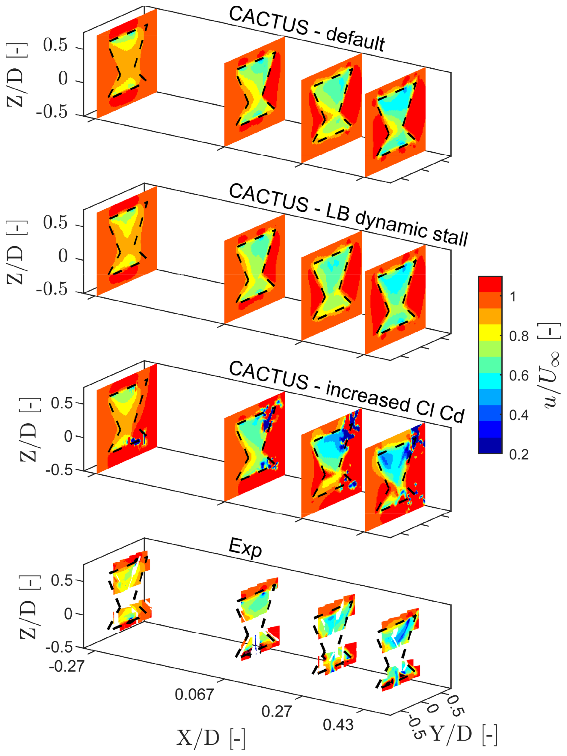
Figure A1 Normalised streamwise velocity ($u/U_{\mathrm{\infty }}$) contours of the X-Rotor at azimuth θ=0° at downstream locations $X/D=-\mathrm{0.27}$, 0.067, 0.27, and 0.43, where D is the rotor diameter for different input conditions. The first tile is the default case, the second tile shows the use of dynamic stall, the third tile shows a case with an artificial increase in C_L and C_D, and the last tile shows the experimental results. The dashed black lines indicate the projected frontal area of the rotor on the corresponding plane. All spatial coordinates are normalised to the diameters D. The x axis is magnified to enhance visibility.

With the introduction of dynamic stall, some flow features that were not captured in the default case are now visible here, and they agree quite well with the flowfield from the PIV results – especially in the most upwind plane. This suggests that the dynamic stall model is essential so as to ensure accuracy in the experiments. With an artificial increase in C_L and C_D of 15 %, there appears to be some instability again, as the vortex core size for that case is small with respect to the vorticity strength it offers. However, we see significant velocity magnitude changes between the default case and this inside the rotor area, even at the most upwind plane. Overall, we understand that any changes to lift and drag still significantly affect the flowfield within the volume of the rotor and that including dynamic stall more accurately represents the flowfield of the X-Rotor.

To identify the influence of the vortex core size, we present the integrated blade forces between the default (now with dynamic stall) and the lowered bound and trailing vortex core radius in Fig. A2.

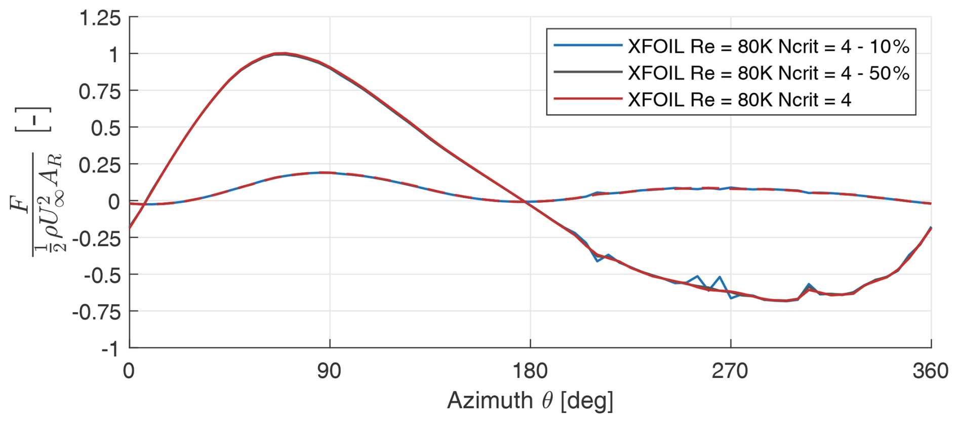
Figure A2 Integrated blade forces F as a function of azimuth θ to show sensitivity to vortex core sizes. The solid lines represent the normal force, and the tangential force is represented by the dashed lines. Positive normal force is away from the axis of rotation and vice versa. Forces are integrated along both upper and lower halves of B1.

Between the default and 50 % reduced vortex core size cases, we see very little difference in the force profiles. While moving down to 10 % core radius, we see minor differences concentrated in the downwind half where blade vortex interaction is expected (around θ=300°). This indicates that the forces, and by extension the wake, is not extremely sensitive to the vortex core size.

To further elaborate on this, we present the spanwise distribution of the forces for the same cases in Fig. A3.

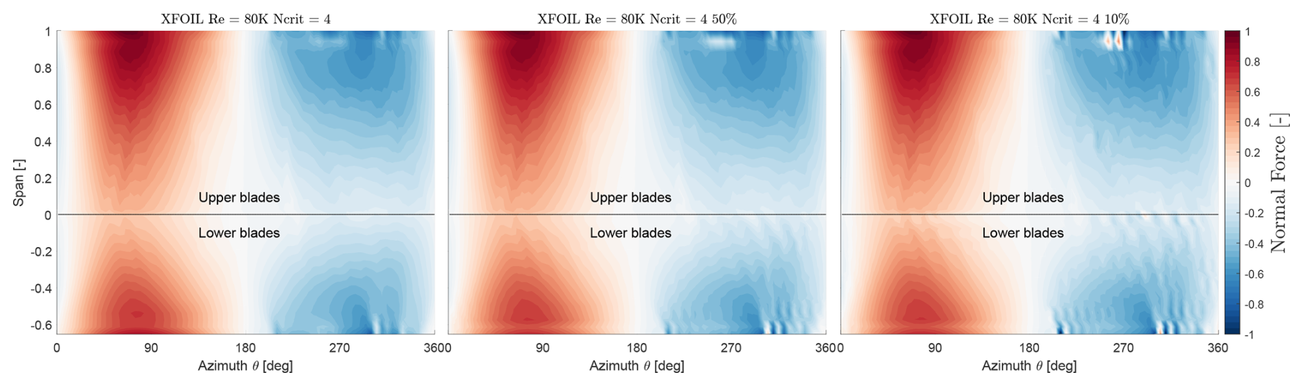
Figure A3 Spanwise distribution of normal blade forces F_N as a function of azimuth θ. Positive normal force is away from the axis of rotation and vice versa.

We see that there are very minor differences between the first two tiles, as observed in the integrated forces. However, we notice that there are some artefacts in the third tile around $Z/D=\mathrm{0.9}$ and exists in the downwind windward regions. This reflects on what we observed earlier, as the difference in the core radius is explicitly visible in the downwind half, where the simulation is approaching instability.

Comparing the velocity fields with 10 % vortex core size and the default at θ=0° (Fig. A4) shows a minor impact in the flowfield; we consider the solver to be relatively independent of the vortex core size.

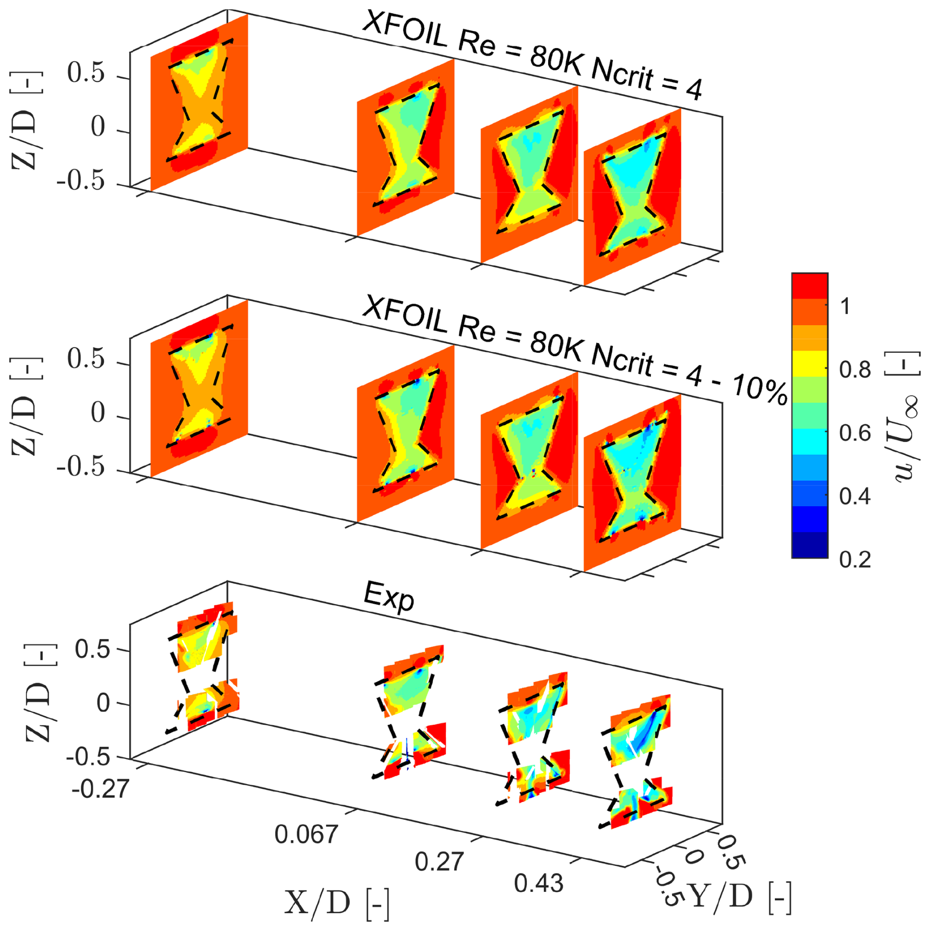
Figure A4 Normalised streamwise velocity ($u/U_{\mathrm{\infty }}$) contours of the X-Rotor at azimuth θ=0° at downstream locations $X/D=-\mathrm{0.27}$, 0.067, 0.27, and 0.43, where D is the rotor diameter for different input conditions. The first tile is the default case, the second tile shows the case with 10 % vortex core size, and the last tile shows the experimental results. The dashed black lines indicate the projected frontal area of the rotor on the corresponding plane. All spatial coordinates are normalised for the diameters D. The x axis is magnified to enhance visibility.

Therefore, given these benefits of using dynamic stall in this analysis, we choose to operate with the Leishman–Beddoes dynamic stall implementation in CACTUS and proceed to use a higher than usual vortex core radius due to the indifference of the blade forces to this parameter.

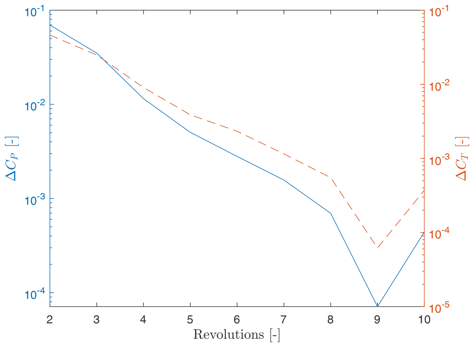
Regarding the convergence of the solution, we chose to opt for 10 revolutions, as it can be seen from Fig. A5 that beyond the eighth revolution, the errors fall below the order of appreciable difference to the results discussed in this study.

Figure A5 Convergence plot of power and thrust. The y axis is in logarithmic scale.