A 3-year database of atmospheric measurements combined with associated operating parameters from a wind farm of 2 MW turbines including rotor geometry

A comprehensive meteorological data set from an operational wind farm, consisting of six 2 MW turbines, has been made available. A meteorological mast, equipped with sonic anemometers at four different heights, was installed at the center of the farm and has collected data over 3 years. The data set is further supplemented with radiometer measurements for atmospheric stability analysis. Simultaneously, supervisory control and data acquisition (SCADA) data were acquired to provide operational information about the wind turbines, including inter alia power production and wind direction. Additionally, the turbine blades were scanned to support aerodynamic simulations. This unique and comprehensive database has been made accessible to the research community through the AERIS platform.

1 Introduction

In this work, we present a database of atmospheric measurements within a wind farm. The database contains environmental data collected over a 3-year period by a meteorological mast (met mast) and a radiometer, both located near an onshore wind farm consisting of six Senvion MM92 wind turbines. Additionally, supervisory control and data acquisition (SCADA) data from four of the six turbines are included for the same period. These data sets together with rotor and blade geometry provide essential information on the operating states of the turbines, enabling the assessment of wind turbine wake dynamics and the associated wake-induced turbulence, through either physical models or numerical simulations.

Depending on wind direction, the met mast is exposed either to undisturbed atmospheric flow or to flow affected by the wakes of the turbines. The met mast is equipped with four sonic anemometers, which allow for detailed measurement of wind speed components and accurate assessment of turbulence and thermal covariances, even in wake-affected conditions.

The originality of the present database is multifaceted:

• Operational wind turbine (SCADA) data. Access to operational data from commercial wind farms is rare, despite the existence of some publicly available databases (Passos et al., 2017; Plumley, 2022; Fraunhofer IWES, 2022). Typically, academic researchers must negotiate agreements with wind farm operators to access such data, with the dissemination of results often subject to industrial approval. By providing this database as open data, we aim to attract the attention of researchers who require full-scale data on turbulence properties and wind turbine operations to validate physical and numerical models at both rotor and wind turbine scales.

• Measurement of wind properties. The wind energy industry typically measures wind properties using cup anemometers or lidar profilers (Duc and Simley, 2022). These sensors, however, are limited in their ability to capture the turbulence tensor and assess the thermal stability of the atmosphere. These limitations are addressed in the present database through the use of sonic anemometers, which enable more comprehensive measurements.

• Expansion of the database. This initial database serves as the foundation for further data sets generated within the same wind farm site. These additional data sets will be collected through two French research projects, ePARADISE and ANR MOMENTA, for which data are available on the AERIS website (https://awit.aeris-data.fr/, last access: 29 August 2025). Future measurements will include data from instrumented unoccupied aerial vehicles (UAVs) and a scanning lidar, complementing the current database.

• Applications and future benchmarking. Some outcomes from this database are already being used by project partners to perform and validate physical and numerical simulations at both rotor and wind turbine scales. When published, the results will provide a valuable basis for broader benchmarking, fostering collaboration with other institutions globally.

2 Description of the site and the farm arrangement

The site under investigation is located near Saint-Hilaire-de-Chaléons in western France, approximately 10 km east of the Atlantic coast and 32 km west of Nantes (see Fig. 1a). It consists of six Senvion MM92 wind turbines, each with a rotor diameter of D = 92 m and a hub height of h_hub = 80 m, as further detailed in Sect. 5. The turbines are arranged in two rows, each containing three turbines, with a row-to-row spacing of 1.2 km (see Fig. 1b). The distance between turbines T1 and T2 and between turbines T2 and T3 is approximately 350 m (equivalent to 3.8D), while the spacing between turbines T4 and T5 and between turbines T5 and T6 is approximately 280 m (equivalent to 3D).

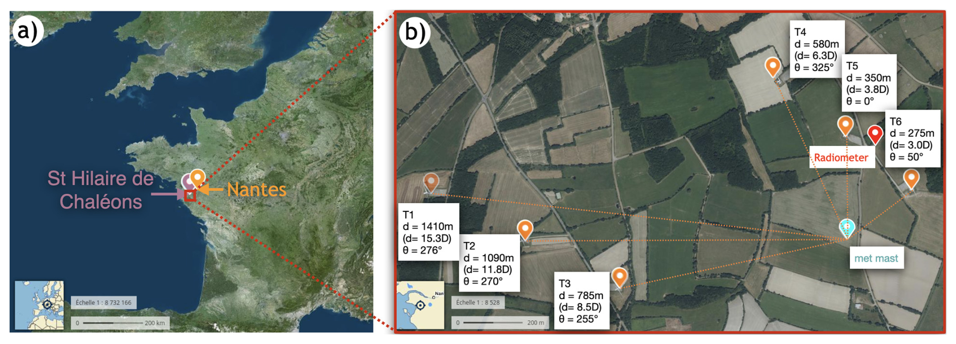
Figure 1 Overview of the measurement site (b) at Saint-Hilaire-de-Chaléons in the west of France (a). The site is 10 km from the coast and 32 km from Nantes. The site consists of six wind turbines with different distances d from the met mast (b). Aerial photo source: © IGN – ≪BD ORTHO^®≫.

A met mast, with a height of 79 m, is positioned between the two turbine rows. It is described in Sect. 3. The distances between the turbines and the met mast are shown in Fig. 1b. The coordinates and terrain elevation above sea level h_asl at each turbine location and the met mast are provided in Table 1. The terrain in the area is relatively flat, with elevation variations of approximately ±1 m between the met mast and turbines T3–T6 (see also Fig. 2). However, turbines T1 and T2 are located 4 m higher than the met mast.

Table 1 Coordinates and elevation above sea level h_asl of the turbines and the met mast.

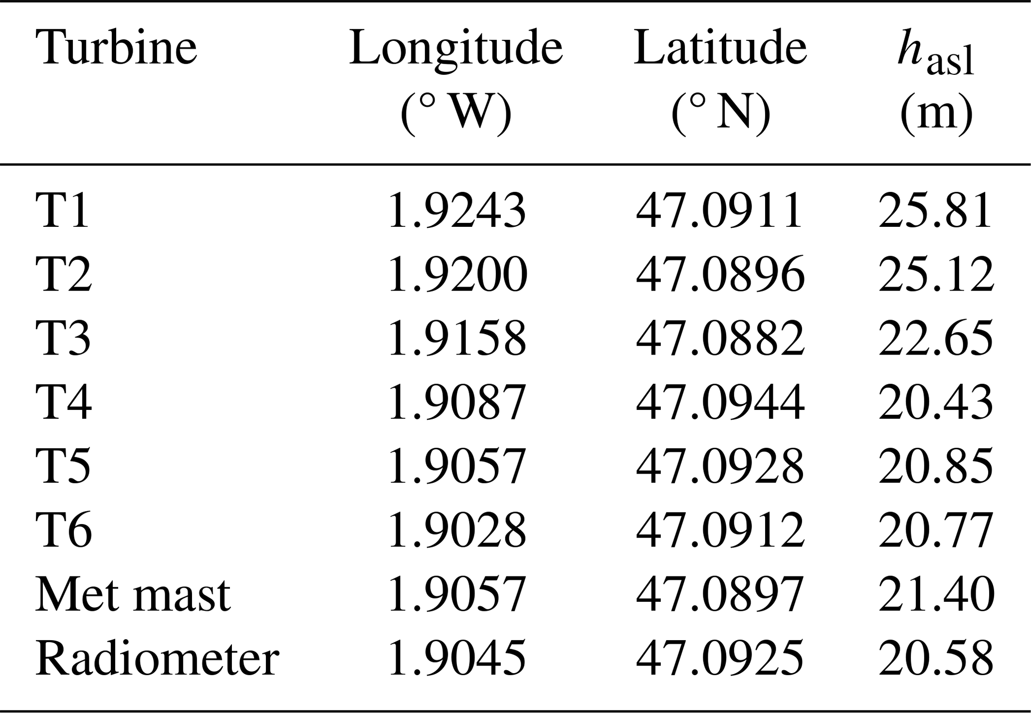
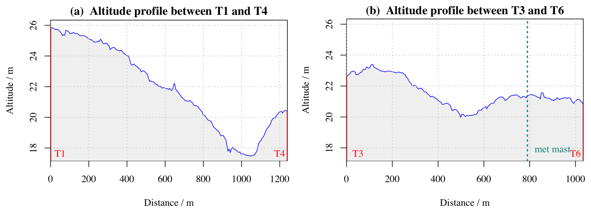
Figure 2 Exemplary terrain elevation profiles between (a) turbines T1 and T4 and (b) T3 and T6. The approximate position of the met mast is indicated; note that the met mast is about 75 m away from the line along which the profile was plotted. Digital elevation model source: © IGN – ≪RGE ALTI^®≫.

A radiometer that is further described in Sect. 4 is installed near turbines T5 and T6 (at a distance of 100 and 197 m, respectively), as shown in Fig. 1b. It is used to capture variability in the vertical structure of the atmospheric surface layer.

Figure 1b presents an aerial view of the terrain at the measurement site. The surrounding area is predominantly flat, consisting of grass fields interspersed with single rows of bushes and trees, which reach heights of approximately 10–15 m. To the northwest of the met mast, behind turbine T6, there are groves where the tree height is similar to that of the field hedges.

3 The meteorological mast

The meteorological mast was installed in the wake of turbine T6 for a northeast wind direction (see Fig. 1). It is a three-legged guyed lattice mast, constructed from 26 triangular sections, each with a height of 3 m and a width of 0.45 m. The guy wires are attached to the legs of the mast and oriented perpendicularly to the opposite side of each triangular section, at angles of 0, 122, and 302°. The guy wires are fixed at seven different heights (9, 18, 27, 39, 51, 63, and 75 m). The four lower levels are anchored at a distance of 22 m from the base of the mast, while the three upper levels are anchored at a distance of 45 m from the base.

The instrumentation was divided into two main stations: a weather station and a turbulence station; cf. Fig. 3b and c. The weather station measures wind speed at three levels (41.3, 53, and 77 m) using three Thies First Class Advanced anemometers (https://www.thiesclima.com/en/Products/Wind-measuring-technology-First-class/, last access: 29 August 2025) (Thies GmbH & Co. KG, Germany). Version 4.3351.00.000 is used at 41.3 m, and model 4.3351.10.000 is used at 53 and 77 m. At the highest level (77 m), a Thies First Class Advanced wind vane is also used to measure wind direction. Atmospheric pressure is measured at 75 m using an AB 60 barometric pressure sensor (Ammonit Measurement GmbH, Germany), and air temperature is measured at the same level using a TPC1.S/6-ME thermometer (https://galltec-mela.de/produkte/pc-me-und-pc-s-me- analoge-stabsensoren-optimiert-fuer-den-aussenbereich/, last access: 29 August 2025) (MELA Sensortechnik GmbH, Germany).

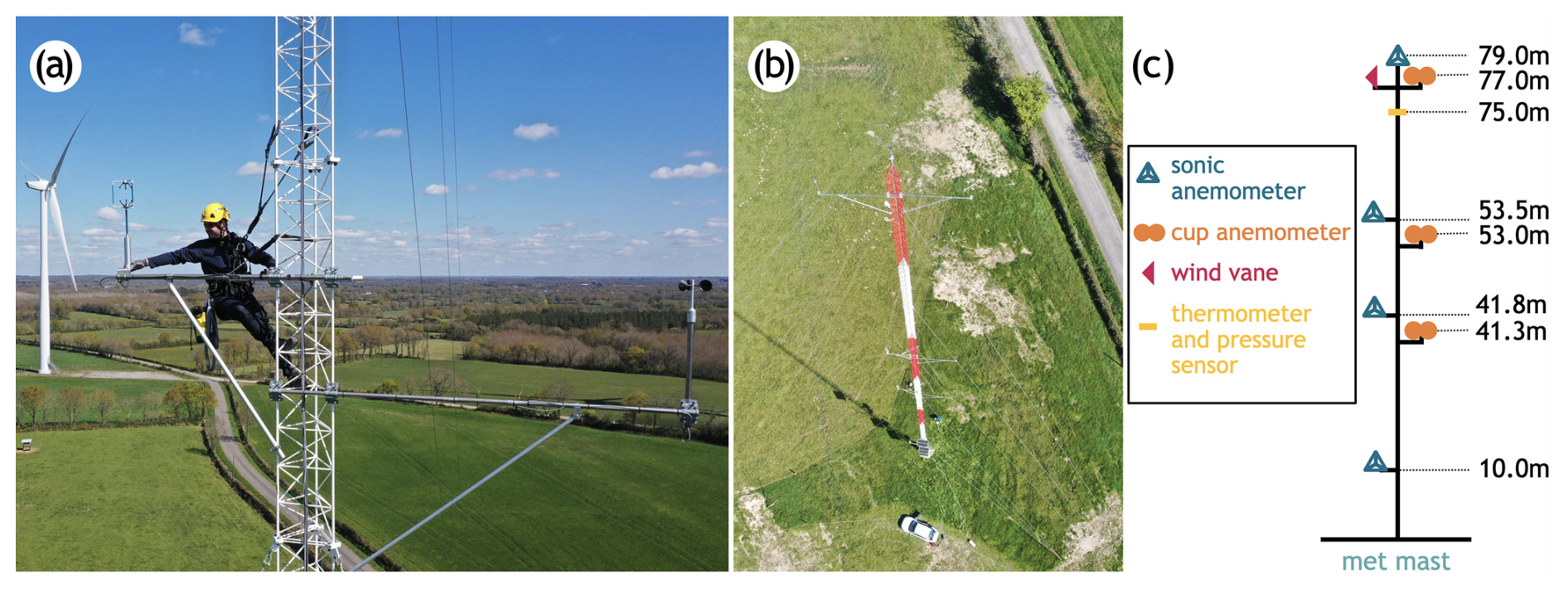
Figure 3 Photographs of the met mast: (a) replacement of a sonic anemometer by a rope technician, (b) the met mast, and (c) sketch of the met mast.

The turbulence station records turbulent velocity components and air temperature fluctuations at four levels (10, 41.8, 53.5, and 79 m) using four WindMaster sonic anemometers (https://gillinstruments.com/windmaster-iss7-datasheet/, last access: 29 August 2025) (Gill Instruments Limited, UK). The lower levels' sonic anemometers (10, 41.8, and 53.5 m) are mounted on a 2 m boom pointing to 302°. This orientation is chosen in order to minimize the time spent in the wake of the mast, as 120° wind does not occur often, as shown by the wind roses. During the field experiment, the top (December 2020) and 41.8 m (February 2022) anemometers were replaced with two Gill WindMaster Pro sonic anemometers due to failure of the installed one. The operation can be seen in the photograph in Fig. 3a of the replacement.

Turbulence measurements were collected from December 2020 to January 2024 at a frequency of 20 Hz to calculate turbulence properties (e.g., turbulence intensities, variances, and covariances) and to perform sensor orientation and calibration corrections using EddyPro^® software (https://www.licor.com/env/support/EddyPro/topics/introduction.html, last access: 29 August 2025). These statistical quantities were computed over an averaging period of 1 h. Figures 4 and 5 show the wind roses and turbulence intensity, respectively, for the measurement period.

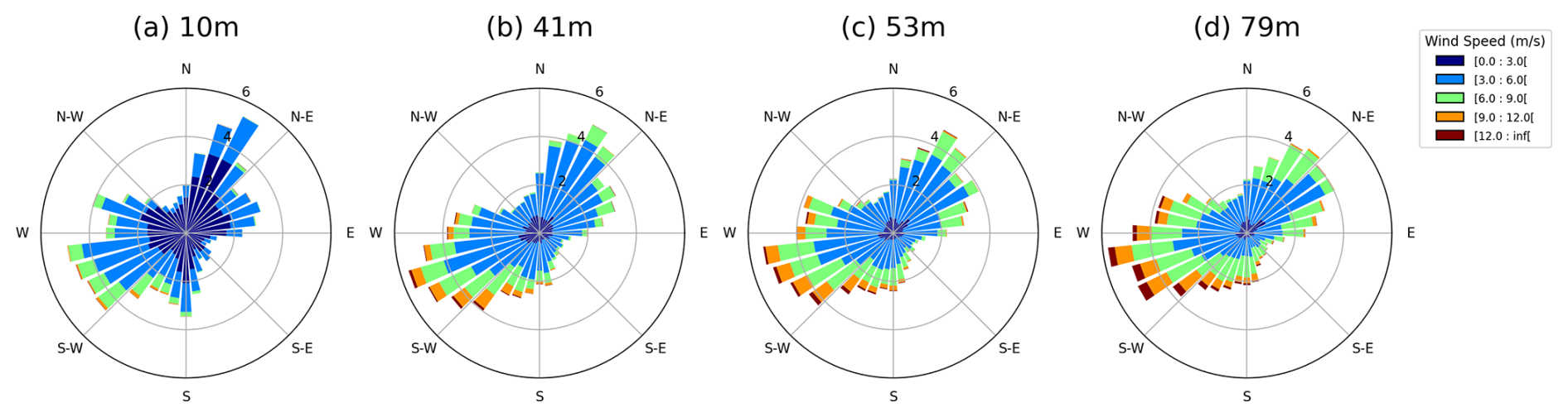
Figure 4 Wind roses obtained from sonic anemometers at heights of (a) 10 m, (b) 41 m, (c) 53 m, and (d) 79 m for 3 years from January 2021 to December 2023.

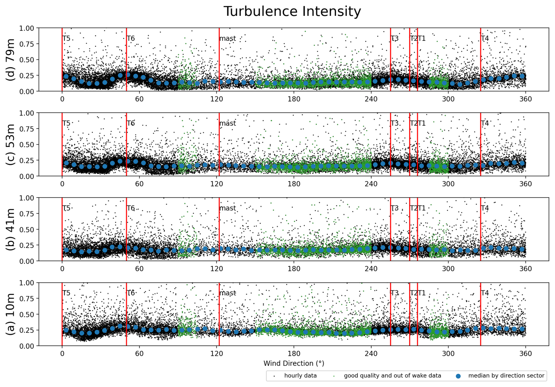
Figure 5 Turbulence intensity obtained from sonic anemometers as a function of wind direction at heights of (a) 10 m, (b) 41 m, (c) 53 m, and (d) 79 m for 3 years from January 2021 to December 2023. Red bars indicate wind turbine locations. Small dots represent hourly data, and big dots are the median values by sector.

The prevailing wind directions are from the west-southwest and northeast. The wind rose distribution is relatively insensitive to altitude, with no systematic veer in the vertical wind profile. However, the wind rose at 10 m shows more scatter compared to the other heights due to the heterogeneity of the terrain in proximity to the ground. Wind speeds at hub height (z = 79 m) typically range from 3 to 12 m s⁻¹, corresponding to the below-rated operational range of the wind turbines.

The turbulence intensity as a function of wind direction exhibits a similar pattern across all altitudes (Fig. 5). It clearly shows higher turbulence intensity at a wind direction of 50°, where the wake of turbine T6 is evident. An increase in turbulence intensity is also observed between 300 and 25°, corresponding to the merged wakes of turbines T4 and T5. The wake effects from turbines T1, T2, and T3 are slightly visible between 240 and 285°. These observations suggest that the atmospheric boundary layer (ABL) turbulence is locally disturbed by wake-induced turbulence from the turbines.

A wake index was defined to identify whether measurements from the sonic anemometer are influenced by wind turbine wakes. The green dots represent wind directions where the met mast is not affected by turbine wakes and where statistical convergence is acceptable (i.e., 90–105°, 150–240°, and 285–300°). In contrast, the black dots indicate wind directions where the met mast is impacted by wind turbine wakes (i.e., 0–90°, 240–285°, and 300–360°) or where the sonic anemometer is in the wake of the meteorological mast (i.e., 105–150°).

Additionally, it is evident that turbulence intensity decreases with altitude for wind directions without wake effects (i.e., interaction between a wind turbine wake and the met mast) in freestream conditions. This trend is less apparent for wind directions experiencing wake interactions. The footprint of wake-induced turbulence on turbulence intensity appears to be less sensitive to altitude.

4 The radiometer

We also operated an RPG HATPRO G2 ground-based passive microwave radiometer (MWR), which has previously been deployed in several field campaigns, including the SOuth West FOGs 3D (SOFOG3D) experiment (Martinet et al., 2022). The radiometer measures the sky brightness temperature at various wavelengths, with a radiometric noise between 0.3 and 0.4 K, using an integration time of 1 s for this experiment. Two frequency bands are utilized by the receivers: the K-band, which targets the water vapor line, with measurements at seven frequencies (22.24, 23.04, 23.84, 25.44, 26.24, 27.84, and 31.4 GHz), and the V-band, which is sensitive to the oxygen line, with measurements at seven frequencies (51.26, 52.28, 53.86, 54.94, 56.66, 57.3, and 58.0 GHz).

Using the inversion algorithm (neural network) described by Rose et al. (2005), the radiometer provides retrievals of water vapor and temperature profiles from the surface up to 10 km altitude, along with measurements of liquid water path and integrated water vapor. The first levels of the vertical profiles are 10, 25, 50, and 75 m above ground level (a.g.l.). Above this, the vertical resolution of the profiles ranges from 30 to 40 m between 100 and 1200 m a.g.l., corresponding approximately to the atmospheric boundary layer. Then, up to 10 km a.g.l., the resolution varies between 60 and 300 m. Retrievals are performed at 93 levels, with a time resolution of 60 s, as outlined by Ricaud et al. (2013). Calibration is performed every five profiles, lasting approximately 4 min.

This ground-based radiometer was deployed from June 2022 to April 2024 as part of the MOMENTA project in the region located at 47.09254° N, 1.90450° W (Fig. 1). It was positioned near turbines T5 and T6 (at a distance of 100 and 197 m, respectively) to capture variability in the vertical structure of the surface layer, depending on whether the measurements were taken within or outside the wake of these turbines. Figure 6 presents a sample of temperature and absolute humidity profiles collected between 15 April and 15 June 2023. A zoomed-in version of these profiles between the surface and 1000 m altitude is shown in Fig. 7, focusing on the period from 22 to 27 April 2023. These profiles clearly demonstrate the daily variation in temperature in the lower troposphere, with a dry period observed around 24 and 25 April 2023, as reflected in the corresponding absolute humidity data. Notably, temperature inversion events (i.e., an increase in temperature with altitude) are consistently associated with the wettest periods.

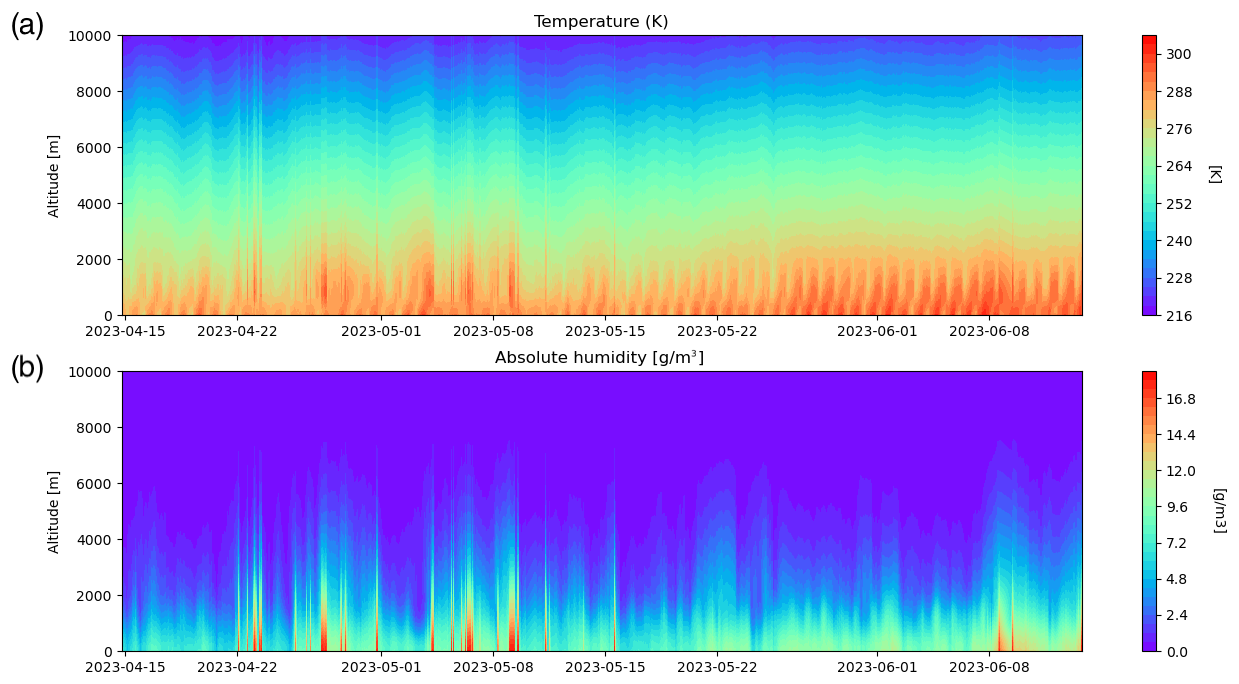
Figure 6 (a) Temperature profiles from the K-band and (b) absolute humidity profiles in g m⁻³ measured between 15 April and 15 June 2023 during the MOMENTA experiment.

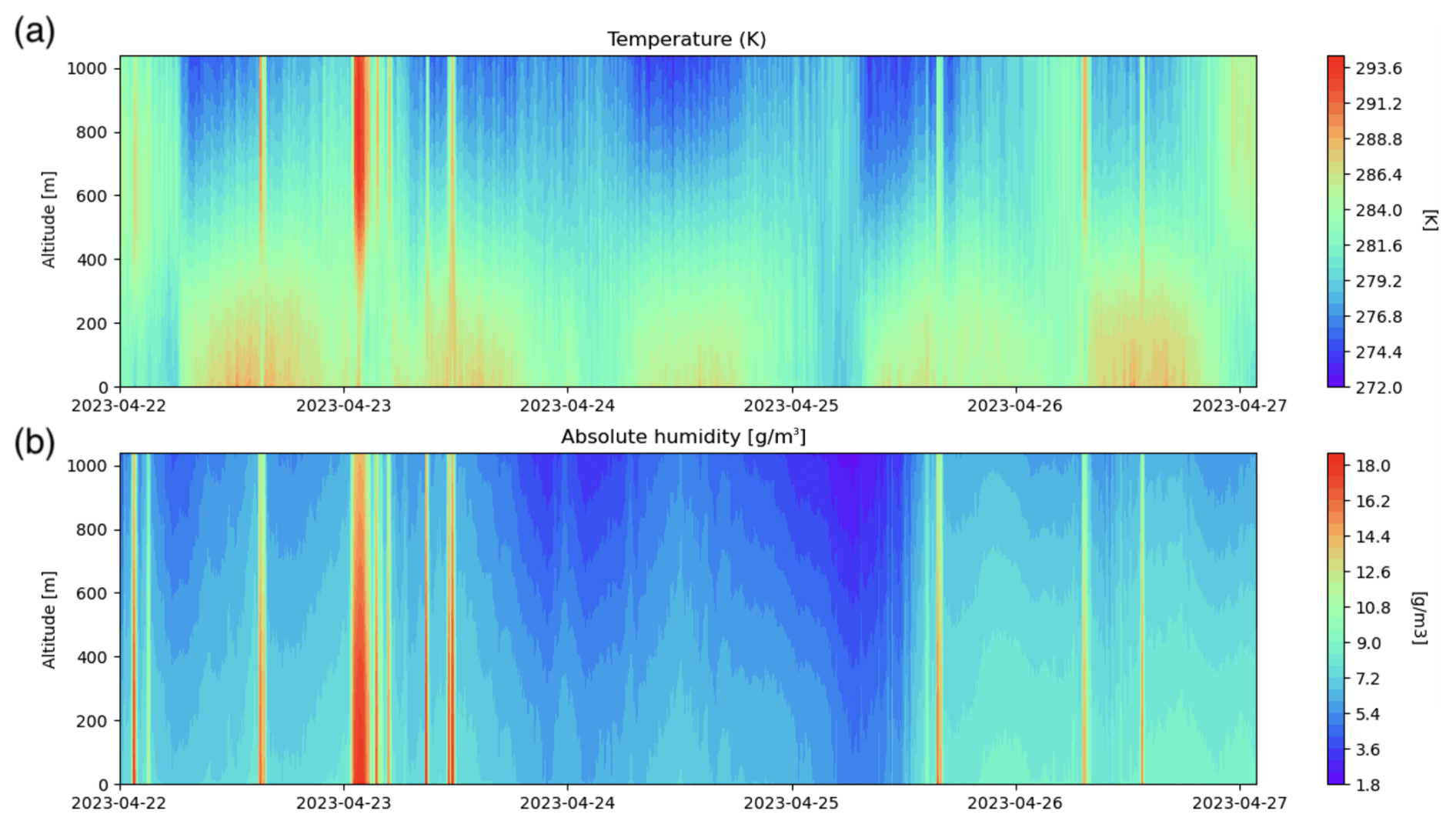
Figure 7 Zoomed-in (a) temperature profiles in the K-band and (b) absolute humidity profiles in g m⁻³ measured in the altitude range of 0–1000 m and between 22 and 27 April 2023 during the MOMENTA experiment.

5 Description of the wind turbine and SCADA data

The wind turbine model used in the wind farm is the MM92, manufactured by Senvion. Figure 8 illustrates the structure of a modern wind turbine similar to the MM92.

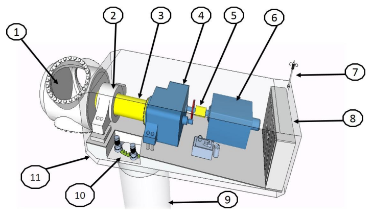
Figure 8 Structure of a modern wind turbine (modified from Lebranchu, 2016), showing the major components: (1) hub or rotor, (2) main bearing, (3) low-speed shaft, (4) gearbox, (5) high-speed shaft, (6) generator, (7) measuring anemometer, (8) transformer, (9) tower, (10) yaw or azimuth bearing, and (11) nacelle.

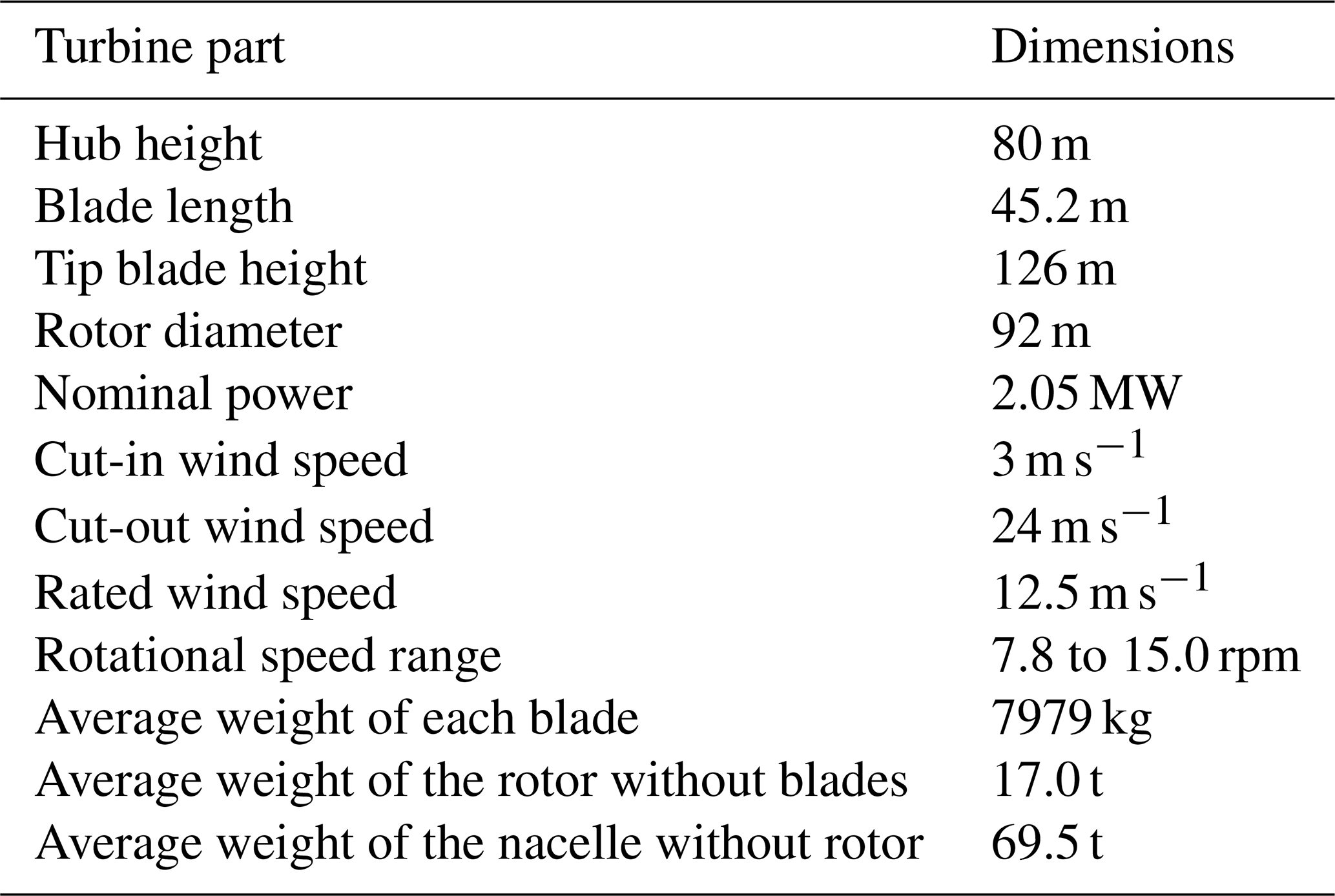
The characteristics of the wind turbines are detailed in Table 2.

Table 2 Characteristics of the wind turbines extracted from technical documents provided by the wind turbine manufacturer at its acquisition.

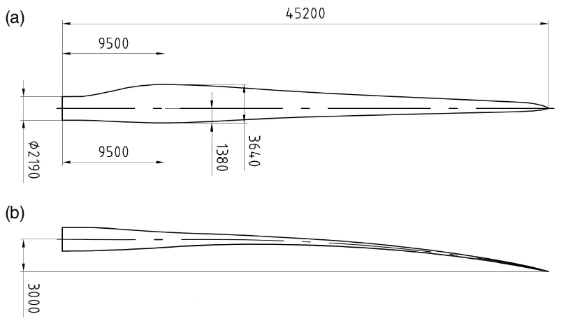
The blade geometry is also documented through scans described in Sect. 6. Figure 9 provides the general dimensions of a single blade.

Figure 9 General dimensions of one rotor blade (in millimeters).

All wind turbines are equipped with a supervisory control and data acquisition (SCADA) system that records 10 min averaged data for various parameters. The data collected are categorized into four main groups:

• 1.

  Environmental parameters.

  • -

    Wind speed. Wind speed is measured using two anemometers mounted on the nacelle, behind the rotor. One is an ultrasonic anemometer with an accuracy of ±0.1 m s⁻¹, used as a reference, while the other is a cup anemometer with an accuracy of ±0.5 m s⁻¹, serving as a backup.

  • -

    Wind direction. Wind direction is determined by combining the nacelle position with the wind vane deviation (measured by the ultrasonic anemometer).

  • -

    External temperature. External temperature is measured using a PT100 sensor located on the nacelle.

  Both wind speed and wind direction are corrected for deviations caused by rotor rotation (which also varies according to wind speed and yaw misalignment), although the transfer functions used for these corrections are not provided by the manufacturer and remain unknown.

• 2.

  Electrical characteristics.

  • -

    Active power. Active power is calculated based on voltage and current measurements.

• 3.

  Control variables.

  • -

    Pitch angle. Pitch angle is measured with an encoder located on the blade control motor, with an accuracy of 0.05° for the blade angle.

  • -

    Low-speed shaft. The rotational speed of the shaft is calculated from pulses generated by an inductive sensor activated by a cogwheel.

  • -

    High-speed shaft. Its rotational speed is measured with an encoder mounted on the generator.

  • -

    Generated torque. Generator torque is derived from the active power measurement and the high-speed shaft rotation.

  • -

    Targeted torque. Targeted torque is obtained from the control algorithms.

• 4.

  Status codes and alarms. These provide detailed information about the operational state of each wind turbine.

6 Extraction of the blade geometry

The blade geometry provided by the manufacturer is incomplete. To supplement data, additional scans were conducted. Numerous approaches and tools are available for blade scanning; in this study, two methods were employed: scanning from the ground and during operational maintenance. Both methods were subcontracted to an expert surveyor firm and utilized the same laser 3D scanning technique, which offers an accuracy of ±3 mm.

Each approach has specific advantages and disadvantages, which are discussed in detail in Sect. 6.1. The post-processing method used to generate point clouds for blade geometry extraction is described in Sect. 6.2. Lastly, the accuracy evaluation of the airfoil shape is presented in Sect. 6.3.

6.1 Scan methods

6.1.1 Scan from the ground

The first scan was conducted from the ground, allowing the blades to remain mounted (see Fig. 10a). However, several drawbacks were identified:

• 1.

  Weather conditions. Despite targeting no-wind conditions, residual wind caused blade movement, increasing the dispersion in the measured point cloud. This variability resulted in the inability to extract a unique blade shape from the data (see Fig. 10b).

• 2.

  Obstructions. Parts of the blades were obscured by the tower during scanning, creating gaps in the measured point cloud (see Fig. 10c). These gaps prevented the complete extraction of the 3D blade properties.

• 3.

  Hub alignment challenges. Determining how the blades were mounted on the hub, including pre-cone and tilt angles, posed additional difficulties (see Fig. 11). Evaluating the tilt angle required scanning the entire nacelle with a reference framework from the ground, while extracting the pre-cone angle necessitated knowledge of the rotor plane. Unfortunately, these parameters could not be derived from the data collected using this scanning method. The origin of the hub framework, essential for determining the pre-cone angle, was also inaccessible.

To address these limitations, a method for extracting the pre-cone angle is detailed in the next section, using data from the second scanning method.

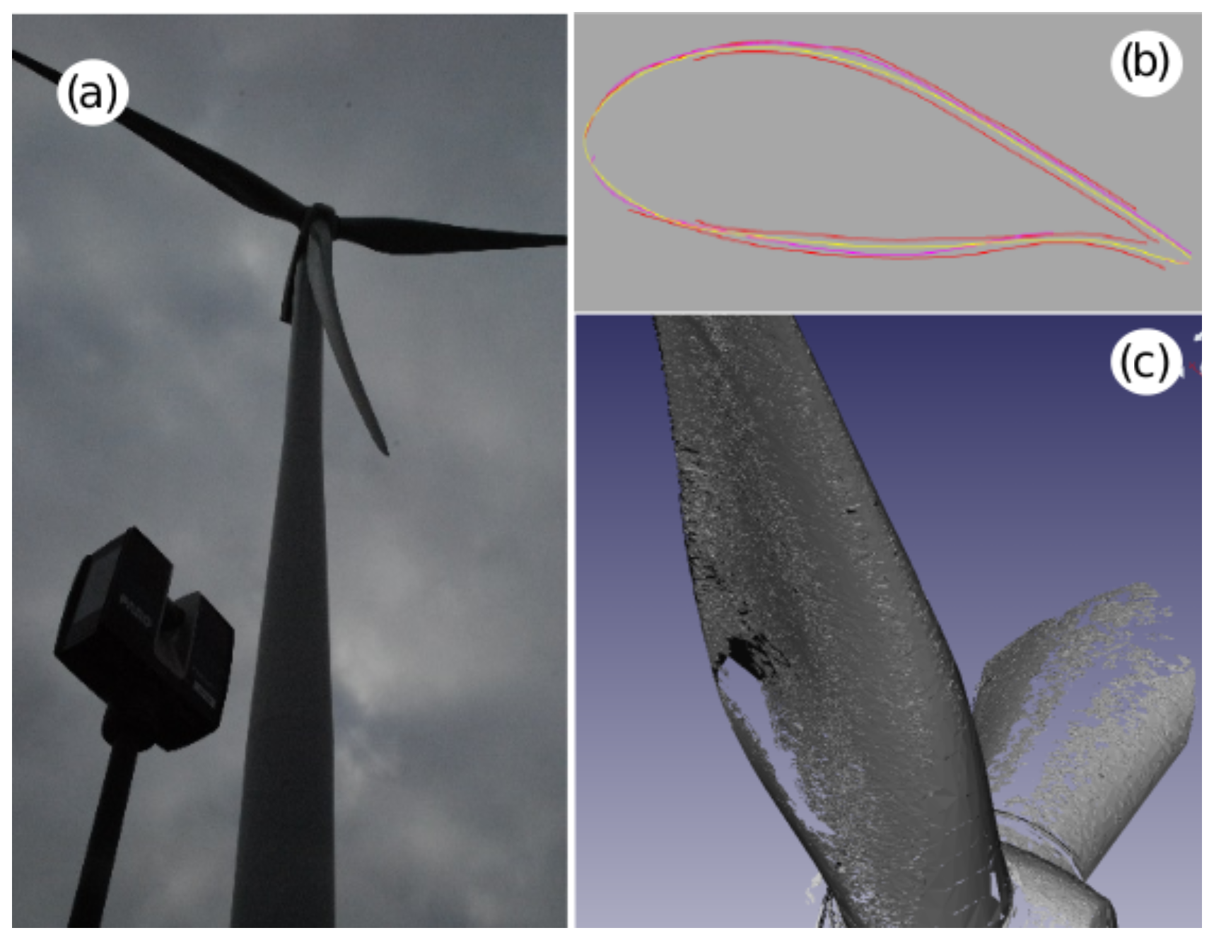
Figure 10 First blade scan operation: (a) 3D scanner on the ground close to the wind turbine, (b) scatter of possible blade sections that can be extracted from the cloud of points, and (c) missing data (“holes”) in the measured cloud of points from this first scan operation.

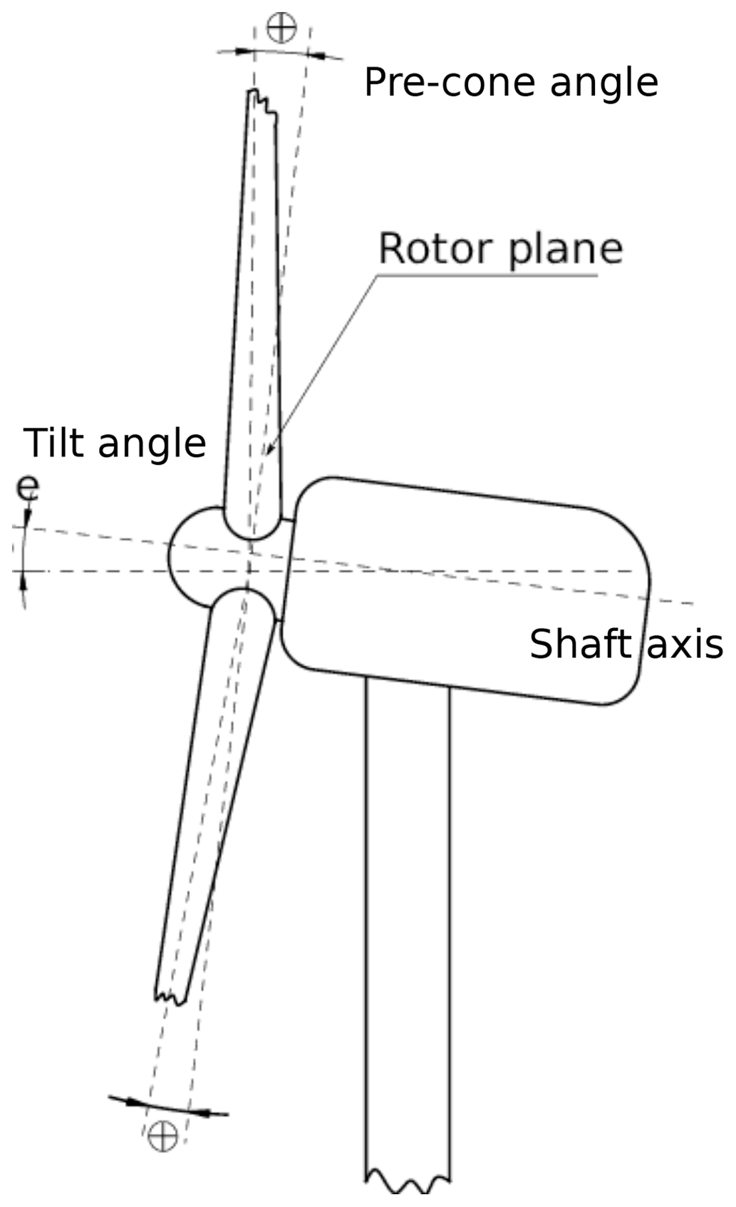
Figure 11 Illustration of the pre-cone angle, i.e., the angle between the root blade axis and the rotor plane, and the tilt angle, i.e., the angle between the horizontal axis and the shaft axis. Sketch modified from Menon Muraleedharan Nair (2017).

Ultimately, one 2D blade section shape at 82 % of the blade length was successfully extracted. To evaluate the aerodynamic loads of this blade section, it was extruded, manufactured, and tested in the Centre Scientifique et Technique du Bâtiment (CSTB) wind tunnel (see Neunaber et al., 2022). Additionally, a 1:10 scale model of this 2D blade section was manufactured and tested in the Laboratoire de recherche en Hydrodynamique, Énergétique et Environnement Atmosphérique (LHEEA) wind tunnel and simulated using unsteady Reynolds-averaged Navier–Stokes (URANS) equations (see Mishra et al., 2024).

6.1.2 Scan during operation maintenance

Another scan of the wind turbine blades was conducted during a rotor bearing maintenance. Compared to the previous method, this approach presented additional challenges:

1. Blade stabilization measures. Devices such as caps at the blade tip and lanyards were used to prevent blade movement (see Fig. 12a and b). While these stabilizers were necessary, they introduced limitations. For instance, the chosen blade had a lanyard at its tip, which obstructed measurements at this location and hindered accurate determination of the pre-bend angle distribution. Additionally, the lanyard was removed during the scan process to accommodate maintenance, leading to increased dispersion in the measured point cloud.

2. Weather conditions. Similar to the first scan method, low-wind conditions were targeted. However, the measured wind speed was 3.57 m s⁻¹ during scanning tests, which causes slight oscillations of the blade tip, thus introducing further dispersion in the measured data.

3. Hub insertion and blade length. The blade extends into the hub at the collar location, a region that could not be captured during the scan (see Fig. 12c). As a result, the total measured blade length was slightly shorter than the actual length provided by the manufacturer (see Fig. 9). The portion of the blade inserted into the hub was estimated to be approximately 0.89 m, as detailed in Sect. 6.2.

Despite these challenges, this scan method included a complete scan of the hub (see Fig. 12d). This allowed the definition of a hub origin, enabling the extraction of the pre-cone angle, as discussed in the next section.

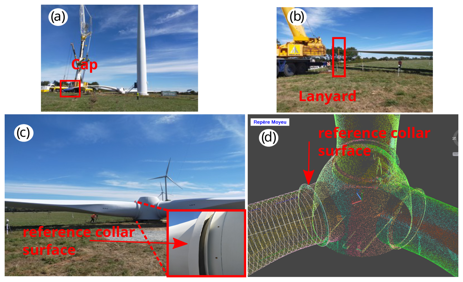
Figure 12 Second scan operation: (a) photograph of the rotor on the ground with caps at the blade tips. (b) Chosen blade for the extraction of the airfoil section; the blade had no cap but was fixed at the ground with a lanyard. (c) Closeup of the blade–hub junction marked by a collar. The collar surface on the blade side was used as a reference for the origin of the blade framework. (d) Measured cloud of points at the hub location with white circles representing the extracted profiles. The first extracted profile was at the reference surface collar on the blade side, with a diameter equal to the collar diameter.

6.2 Post-processing of blade scan data

Because the second scanning strategy provided more comprehensive data, it was used to extract the blade geometry, following the procedure outlined below.

6.2.1 Hub and blade frameworks

Blades are elastic and are typically mounted at a predefined angle relative to the rotor plane – the pre-cone angle – to prevent contact with the tower during operation (see Fig. 11). To determine this pre-cone angle, the hub framework must first be defined (see Fig. 13a and b).

The blade framework originates at the blade–hub junction, with its origin, O_blade, located on the blade root axis. The framework axes are detailed in Fig. 13c.

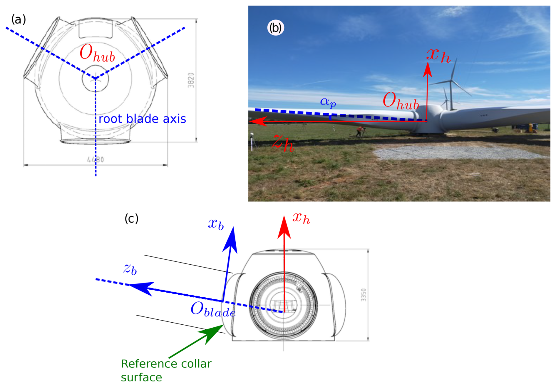
Figure 13 Definition of the coordinate framework of the blade (measurements are in millimeters): (a) front view of hub. Dotted blue lines indicate the blade axes at the root location. The intersection of the three blade axes defines the hub framework origin, O_hub. (b) The z_h axis is parallel to the ground; x_h is normal to z_h and towards the sky; and y_h is such that the hub framework is an orthogonal, right-handed one. α_p is the pre-cone angle, defined as the angle between the root blade axis and the z_h axis. (c) Side view of the hub. The blade framework origin is the center of the circular blade root section, O_blade (i.e., on the blade root axis), and starts at the reference collar surface; y_b is parallel to the chord direction of the largest blade chord (see Fig. 14); and x_b is such that the blade framework is an orthogonal, right-handed one.

The distance between the hub and blade origin is 2 m, corresponding to a translation of the hub framework by

• dx_h = 0.140 m,

• dy_h = 0.043 m,

• dz_h = 1.998 m.

The pre-cone angle was calculated to be 3.8°, which is slightly higher than the manufacturer-specified value of 3.5°.

6.2.2 Extraction of blade sections

Once the blade framework was established, blade sections were extracted along the sweep and pre-bend lines (see Fig. 14). This process was performed manually: when z_b deviated from the blade root axis, y_b was adjusted along the local chord axis based on the identification of the leading and trailing edges. This approach ensured that the extracted sections were normal to the sweep and pre-bend lines.

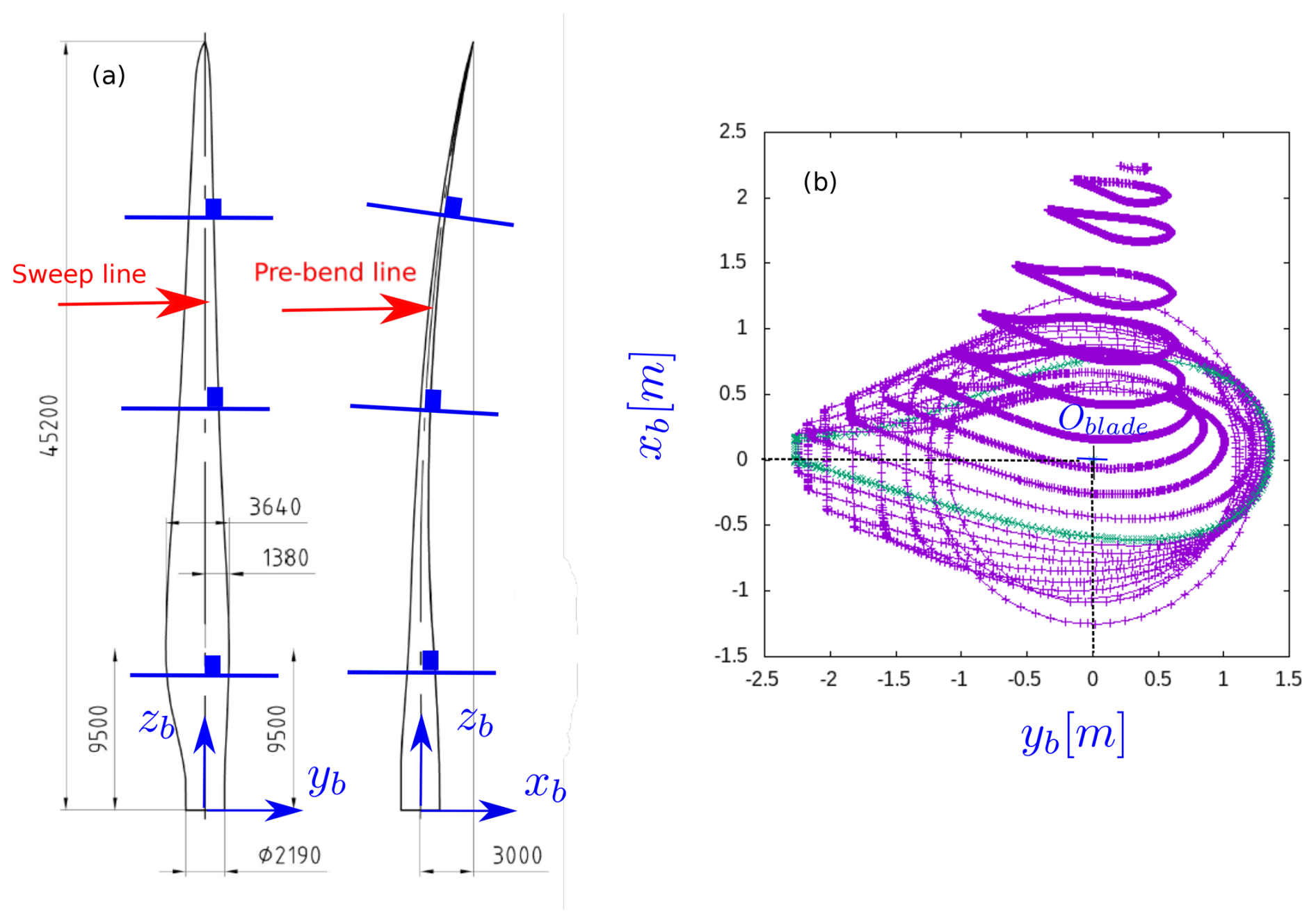
Figure 14 Extraction of blade sections (measurements are in millimeters): (a) extraction of blade section along the sweep and pre-bend lines; (b) 45 sections along the blade were extracted. The green section has the maximum chord, and its orientation is used to define the y_b axis.

Blade sections were extracted at intervals of 200 mm, resulting in a total of 223 profiles. However, some profiles were excluded due to evident inaccuracies or because they coincided with the lanyard's position. A subset of 45 sections was deemed sufficient to describe the sweep and pre-bend lines, the local twist angle, and the airfoil sections forming the blade (see Fig. 14).

For further details on the resulting distributions, readers can refer to Dubois et al. (2022). The chord and thickness distributions showed very good agreement with the manufacturer's specifications. However, the pre-bend line was found to be less accurate, likely due to blade deformations caused by the lanyard used to stabilize the blade during the scan.

6.3 Accuracy of blade sections and loads

Airfoil sections composing the blade were not provided by the manufacturer, limiting the evaluation of scanning accuracy. Nevertheless, a partial accuracy assessment was performed using data from the two scanning methods. For this purpose, the blade section at 82 % of the blade length was extracted from both scans and compared in terms of shapes.

The blade shapes, shown in Fig. 15a, were found to be highly similar, with a maximum difference of 2 mm on the pressure side – well within the measurement accuracy. The reader can find load evaluations at the chord-based Reynolds numbers¹ $R{e}_c=\mathrm{4.7}\times {\mathrm{10}}^{\mathrm{6}}$ and $R{e}_c=\mathrm{3.6}\times {\mathrm{10}}^{\mathrm{6}}$, from experiments at full chord length performed in the CSTB wind tunnel (Neunaber et al., 2022; Braud et al., 2024). Experiments and simulations were also performed at scale 1:10, $R{e}_c=\mathrm{2}\times {\mathrm{10}}^{\mathrm{5}}$, using LHEEA's wind tunnel and the ISIS-CFD² software (Mishra et al., 2024).

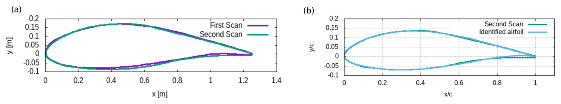
Figure 15 Airfoil section accuracy evaluations (more details on the airfoil shapes can be found in Table 3). (a) Comparison between airfoil shapes from first and second scan. (b) Comparison between the identified airfoil shape (i.e., modified NACA 63(3)418) and the second scan shape.

The airfoil properties derived from the scans were sufficiently accurate to identify the NACA³ airfoil family and its associated aerodynamic characteristics. The blade section closely resembles a NACA 63(3)418 profile, a NACA profile shape referenced in the available NACA database (https://m-selig.ae.illinois.edu/, last access: 29 August 2025), with a modified thickness⁴ and a modified camber⁵ (see Table 3). For such profiles, a trailing-edge stall process is expected, as described by Gault (1957). This profile shape also exhibits local load bi-stability near the maximum lift value, as demonstrated experimentally by Neunaber et al. (2022) and Braud et al. (2024) for a full-scale chord-based Reynolds number corresponding to that of a 2 MW wind turbine. The presence of stall cells was evidenced numerically at the 1:10 scale by Mishra (2024).

Table 3 Airfoil shape characteristics: the columns contain the airfoil maximum thickness and its location in a percentage of the chord and the maximum camber and its location in a percentage of the chord. The first two rows of this table show the airfoil properties for the two scanned cases, while the third row corresponds to the original (unmodified) NACA profile shape, namely a NACA 63(3)418 profile, as a reference. The fourth row corresponds to a NACA 63(3)418 profile modified in such a way that it fits the scanned data.

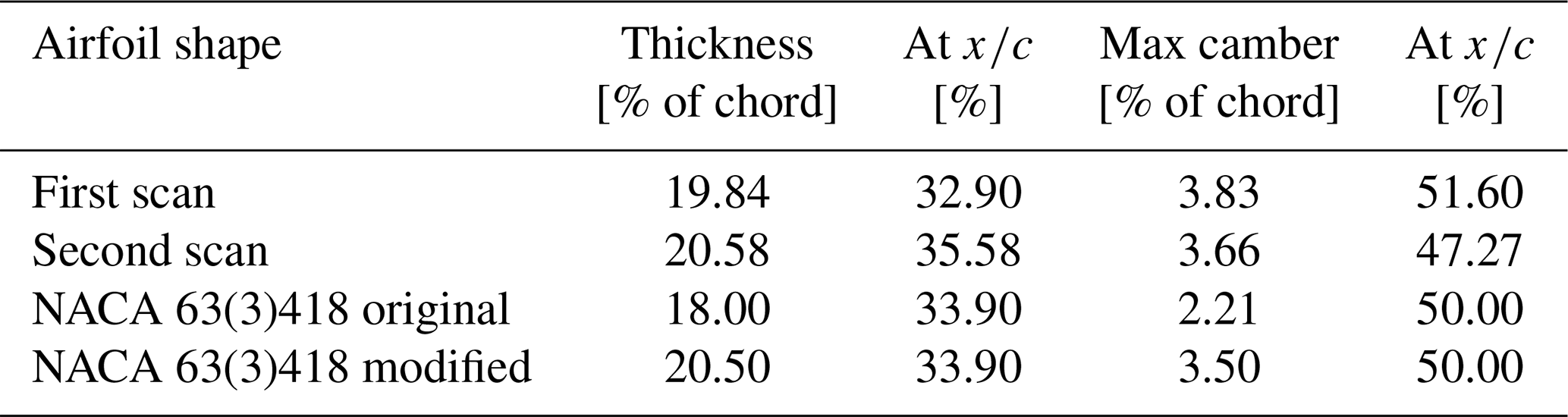
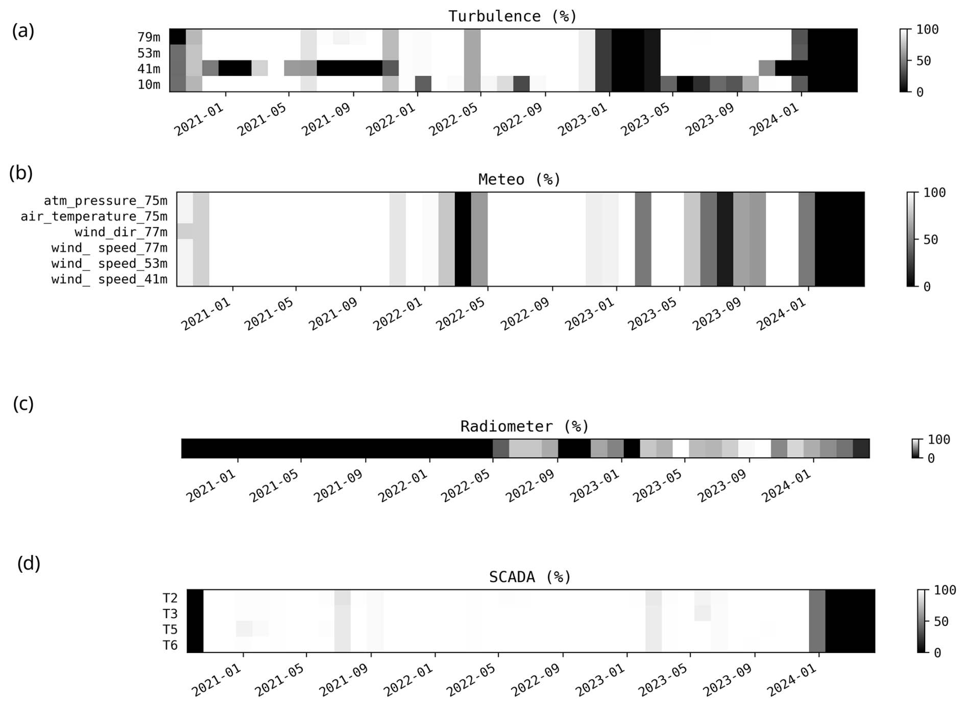
Figure 16 Data availability for the measurement period from December 2020 to January 2024: from (a) the sonic anemometers (“Turbulence”), (b) meteorological sensors on the mast (“Meteo”), (c) the radiometer (“Radiometer”), and (d) the SCADA system of the wind turbines (“SCADA”).

7 Data-set format and organization

• Meteorological mast data sets are stored in CSV format and organized in three directories: “data availability”, “meteo”, and “turbulence”. The “data availability” directory provides availabilities of the meteorological data sets in CSV format (also shown in Fig. 16). The “meteo” directory contains atmospheric data from cup anemometers, a wind vane, a thermometer, and an atmospheric pressure sensor. The “turbulence” directory contains the sonic anemometer measurements at the four meteorologic mast heights detailed in the README file.

• Radiometer data sets are stored in NetCDF format and organized in four directories: the CMP.TPC folder contains atmospheric temperature profile data collected over time. The file includes time-indexed measurements across 93 altitude layers, along with metadata and rain flag. The HPC folder contains vertical profiles of absolute and relative humidity collected over time across the atmospheric layers. The data include metadata on measurement conditions and auxiliary quality indicators such as rain detection. The IWV folder contains time-resolved measurements of integrated water vapor (IWV), along with viewing geometry, retrieval method, and rain flag. The MET folder contains NetCDF files of meteorological measurements (observed at 3 m a.g.l.), including pressure, temperature, and relative humidity at a temporal resolution of 1 s. Each entry corresponds to a single point in time and includes metadata such as rain status and integration details.

• SCADA data sets are stored in CSV format and organized in three directories: the “DATA” directory contains the CSV files, the “AVAILABILITY” directory provides availabilities of SCADA data (also shown in Fig. 16 of the paper), and “MANUFACTURER-INFORMATION” contains the power and thrust curves. For reasons of confidentiality, the data are available for four of the six turbines only. More details on the data organization can be found in the README.txt file.

• The blade scan data can be read using the CSV format as performed in the provided Python code “plot-3DBlade.py”. The README.txt file explains the content of the directory, including filenames “Rxxm.txt”, which contain the 2D airfoil profiles composing the 3D blade.

8 Conclusions

A comprehensive meteorological data set from an operational wind farm, consisting of six 2 MW turbines located in Saint-Hilaire de Chaléons, Pays-de-Loire (commercially operated by VALEMO/VALOREM), has been made available. A meteorological mast was installed at the center of the farm and has collected data over 3 years, equipped with sonic anemometers at four different heights.

The data set is further supplemented with radiometer measurements conducted from 15 June 2022 to 16 April 2024, for atmospheric stability analysis. Simultaneously, SCADA data were acquired to provide operational information about the wind turbines, including power production, wind direction, and other key parameters. In addition, the turbine blades were scanned to support aerodynamic simulations. This unique and comprehensive database has been made accessible to the research community through the AERIS platform.