Wind turbine wake detection and characterisation utilising blade loads and SCADA data: a generalised approach

Large offshore wind farms face operational challenges due to turbine wakes, which can reduce energy yield and increase structural fatigue. These problems may be mitigated through wind farm flow control techniques, which require reliable wake detection (recognising the presence of a clear wake) and characterisation (parametric description of a wake’s properties) as prerequisites. This paper presents a novel three-stage framework for generalised wake detection and characterisation. First, a regression model utilises blade loads, pitch and rotor rotational speed data to estimate the wind speed distribution across the rotor plane. Second, a convolutional neural network undertakes pattern recognition analysis to perform wake detection, classifying rotor-plane wind estimates as “fully impinged”, “left impinged”, “right impinged” or “not impinged”. Third, where wake impingement is detected, two-dimensional Gaussian fitting is undertaken to provide a parametric wake characterisation, providing outputs of the wake centre location and wake lateral width. The framework is trained and tested in a simulation environment incorporating the Mann turbulence model, the dynamic wake meandering (DWM) model for generating wakes and an industrial-grade aeroelastic solver. The testing is undertaken under a wide range of wind conditions, with mean ambient wind speeds from 5–15 m s⁻¹, turbulence intensities from 3 %–9 % and a full range of wind directions. Results show high accuracy of wind field estimation, with the mean RMSE across all test cases being 3.7 % when normalised by mean ambient wind speed. The wake detection model accurately identifies the presence of a wake for approximately 77 % of tested wind fields, with subpar performance observed for more extreme conditions or those at the limits of the training data used. The final wake characterisation stage is shown to flexibly adapt to changing wind conditions, successfully tracking the wake's position even for more turbulent conditions. The proposed framework therefore demonstrates strong potential as a generalised approach to wake detection and characterisation.

1 Introduction

The wind industry has advanced significantly in recent years, reaching a total worldwide installed capacity of 906 GW at the end of 2022 (Hutchinson and Zhao, 2023). Despite being a mature field, some challenges still remain to be solved. Due to the increasing size of modern wind farms, there is a newly posed challenge of effectively operating clusters of hundreds of multi-megawatt machines. For this reason, the current focus for both research and industry is shifting towards a farm-level approach for operations, control and maintenance.

A wind turbine interacts with the incoming wind flow, extracting energy and creating a wake: a downstream region of decreased wind speed and increased turbulence. Due to their varied impact on the farm's performance, wakes play a crucial role in turbine operation. A turbine affected by wakes from upstream machines has a lower energy yield due to a wake-generated velocity deficit in the upcoming flow (Adaramola and Krogstad, 2011; Barthelmie et al., 2010). Having the rotor experience a more turbulent wind field leads to uneven aerodynamic loading on the machine, inducing severe fatigue cycles in its structure (Churchfield et al., 2012). A turbine under waked flow conditions is also prone to experiencing additional loads due to large-scale motions of wake meandering, further enhancing its fatigue (Madsen et al., 2010; Larsen et al., 2013).

Via various control techniques it is possible to mitigate the negatives of waked flow conditions, optimising turbine operation for reliable and effective performance. The earliest developments in this area likely date back to a study by Steinbuch et al. (1988), where the authors implement axial induction control to increase the energy yield by reducing wake effects. Numerous methods for optimising wind farm flow follow; some examples include wake steering by introducing yaw offsets (Howland et al., 2020; SGRE, 2019) or dynamic individual pitch control (Frederik et al., 2020) and dynamic induction control (Munters and Meyers, 2018) to induce enhanced mixing in the wake.

To use the above-mentioned approaches in a closed-loop control scheme, dynamic information on whether the impinging wake is being successfully redirected or dispersed is required (Raach et al., 2016). Moreover, before starting the control action, there first needs to be confirmation that a turbine is indeed wake-affected to facilitate an intervention to its normal operating cycle. For the sake of the discussion in this work, we refer to these two flow control prerequisites as wake detection and wake characterisation. The former refers to the action of recognising that a given turbine is experiencing a clear wake impingement from a nearby machine, in such a way that it has a significant (in both magnitude and time) influence on its performance. The latter refers to the action of identifying the properties of the wake using a simplified parametric representation and monitoring how the values of these parameters change in time.

There is a growing effort in the research community to develop new wake detection and characterisation techniques. Up-to-date approaches focus on implementing remote sensing techniques or using a turbine's operational data. The former is usually achieved with the use of light detection and ranging (lidar) devices, with recent literature featuring numerous examples of their successful application in wake characterisation (Bingöl et al., 2010; Trujillo et al., 2011; Conti et al., 2020; Lio et al., 2020). A recent study (Raach et al., 2016) investigates the use of lidar-based wake characterisation directly in a closed-loop wake steering scheme, showing promising results. Despite achieving good performance, the lidar-based approaches unavoidably rely on additional hardware, which is not currently present at most wind farms and represents a significant additional cost. A different way of tackling the problem is to employ the relationship between the wind field and turbine response. The basic idea behind this approach is that a variation in the incoming flow can be correlated with changes in signals such as blade root bending moments and generator speed. The widely discussed method introduced by Bottasso and Schreiber (2018) relies on using out-of-plane blade root bending moments to approximate the local wind speed in each of the rotor quadrants, thus allowing for partial wake detection. The method is tested in the field (Schreiber et al., 2020) using a setup of two wind turbines and a met mast, providing a proof of concept for the qualitative wake detection. The idea of mapping between the blade loads and local wind speeds has also been used by others; some examples include studies by Kim et al. (2023), Simley and Pao (2016), and Liu et al. (2021). A study by Onnen et al. (2022) pushes this approach further, implementing out-of-plane blade loads to achieve accurate characterisation of the meandering wake deficit with the use of an extended Kalman filter (EKF). The authors also discuss the potential of using the estimation uncertainty metric to detect the wake presence. The method is validated via wind tunnel (Onnen et al., 2023) and field (Onnen et al., 2025) experiments, showing a strong correlation between the estimated wake position and the reference lidar measurements. A similar blade-load-based approach is also considered by Dong et al. (2021), where the authors investigate wake characterisation with an EKF setup within a simulation environment. In another study by Farrell et al. (2022), the authors implement a recurrent neural network trained with experimental and simulation data to estimate the lateral position of the wake centre.

All in all, we identify the research gap as follows: existing wake estimation methods primarily focus on the wake characterisation aspect, with both lidar- and load-based approaches offering high accuracy. Up-to-date wake detection studies have analysed wake impingement in a scenario with a single upwind turbine at a fixed distance, for a fixed set of wind directions. This handles only part of the overall problem in a realistic setting, where the turbine experiences a full range of wind directions. For the majority of inflow angles, the turbine is not directly affected by a nearby turbine's wake; it does however receive a large amount of random flow fluctuations due to operating in the highly turbulent atmospheric boundary layer. Without robust knowledge of whether the turbine operates under wake impingement or not, there is a risk of implementing a wake characterisation scheme on a naturally occurring turbulent eddy, hence providing incorrect and misleading inputs to the control system.

In this paper, we seek to bridge the above-identified gap by proposing a generalised three-stage approach that performs wind field reconstruction, wake detection and wake characterisation within a single framework. Firstly, the instantaneous wind field interacting with the rotor is estimated using turbine operational and load data. Secondly, a neural network approach is implemented to classify whether the estimated wind field represents a case of “full”, “partial” or “no” wake impingement. Thirdly, if clear wake impingement is detected, a parametric wake model is fitted in order to characterise the centre and lateral width of the currently observed wake. A novel end-to-end methodology is presented, which aims to provide both a demonstrator and a performance benchmark for generalised wake detection and characterisation methods of this type. The trained models are tested across a full range of wind directions within a virtual offshore wind farm, evaluating the method's performance for wakes shed at various upstream distances. The simulation environment incorporates Mann turbulence wind boxes, the dynamic wake meandering (DWM) model for generating wake interactions and aeroelastic code to compute the turbine response. This work focuses on developing a novel solution that can confidently assert when a turbine is impinged by a wake from a nearby machine – a key factor for farm-wide wake steering control.

The paper is structured as follows: Sect. 2 discusses the methodology used for the framework's development and training; Sect. 3 presents the results of the framework validation; Sect. 4 considers the discussion on the framework applicability and limitations; and, lastly, Sect. 5 covers the conclusion and addresses future work.

2 Methodology

Section 2.1 discusses the layout of the developed framework and its high-level characteristics. The details of the implementation are described in Sect. 2.2 to 2.5.

2.1 A summary of the proposed framework

Figure 1 shows the information flow between the models within the proposed wake estimation framework. Figure 2 presents two examples that illustrate the framework's performance when (a) the wind field does not have a clear wake impingement from a nearby turbine and (b) when it does. The high-level details on the individual models that the framework consists of are discussed in the following.

Figure 1 A flowchart describing the proposed wake estimation framework.

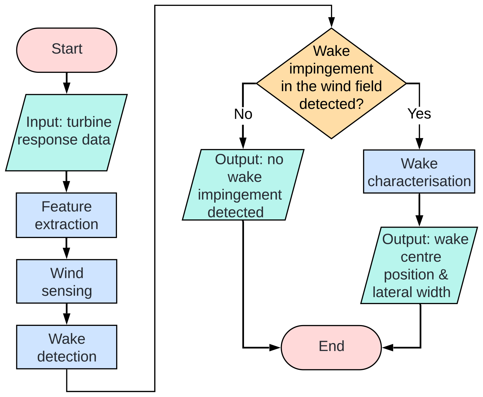
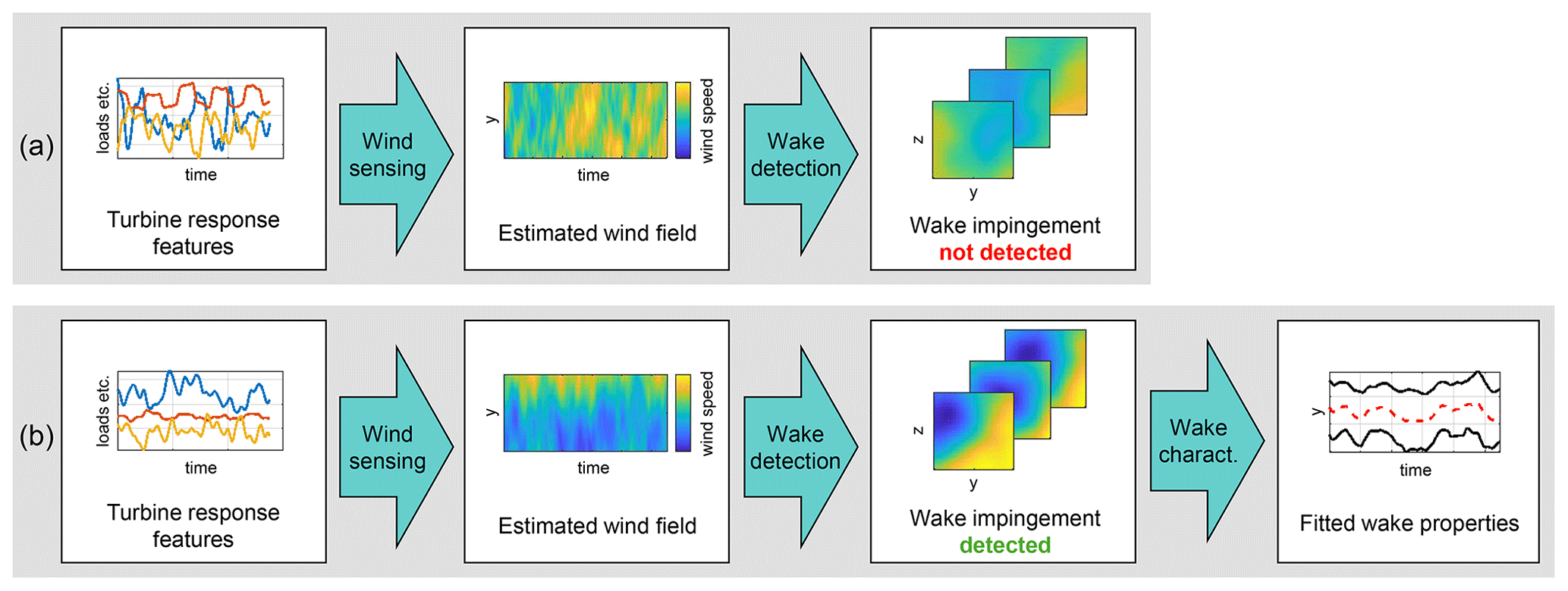
Figure 2 Two examples showing the framework's performance. (a) The incoming wind field does not have a clear wake deficit; thus the framework does not go into the wake characterisation. (b) There is a clear wake deficit; thus the final step of wake characterisation is implemented.

The first constituent model in the developed framework is a wind field estimator, which, when provided with turbine response time series as the input, is capable of producing the wind field reconstruction, thus showing the flow at the rotor as the output. This process is hereafter referred to as wind sensing. A successfully generated wind field estimation provides sufficient information to analyse the flow field and extract the desired wake impingement information. For this framework, we propose performing wake detection using a convolutional neural network (CNN), which, after being trained, can distinguish flow with a well-defined wake deficit from a nearby turbine. If a likely wake impingement is detected, a suitable algorithm aiming to estimate the wake's properties is to be implemented. The ultimate framework output data are two time series of the wake centre position and wake lateral width, describing the horizontal distance where the degree of wake impingement is significant. The combination of these two time series provides a simplified two-dimensional representation of a meandering wake deficit. This representation can serve as an input to wind farm flow control techniques that are informed by the lateral properties of the impinging wake, such as those that use yaw as a control action (Howland et al., 2020; SGRE, 2019). Focusing specifically on the lateral properties is also motivated by the fact that the wake meandering is more pronounced in the transverse direction than in the vertical direction, with the ratio reflecting the turbulence intensities of the respective components (Yang and Sotiropoulos, 2019). The developed methodology also allows us to extract a time series of a peak wake deficit ΔU value; however this is not discussed in this work.

2.2 Framework implementation: training data acquisition

The simulation environment allows the modelling of the operation of a given turbine at any location within the wind farm layout, capturing wake impingement effects from multiple turbines simultaneously. While this aspect plays a key role during testing, training is limited to interactions between two devices located on the farm border: a first-row wake “emitter” and a second-row wake “receiver”, spaced approximately 6 rotor diameters apart. The role of the “receiver” is to provide the turbine response data for training. Four wind directions, representing four distinctive wake impingement scenarios, as seen from the front of the rotor, are defined as follows: (a) fully impinged, with the turbine directly downstream of the closest neighbour; (b) partially impinged, with the wake impacting the left side of the rotor; (c) partially impinged, with the wake impacting the right side of the rotor; and (d) no impingement. The wind direction differs by 5° between the fully and partially impinged cases. This setup allows us to clearly differentiate between the effects of full and partial wake impingement and standalone atmospheric turbulence. It ensures that only one wake impacts the “receiver” turbine; including multiple wakes would complicate the impingement effects and make it more challenging to define wake detection classes (see Sect. 2.4). The partial layout of the wind farm and the wind directions defining the four classes are shown in Fig. 3.

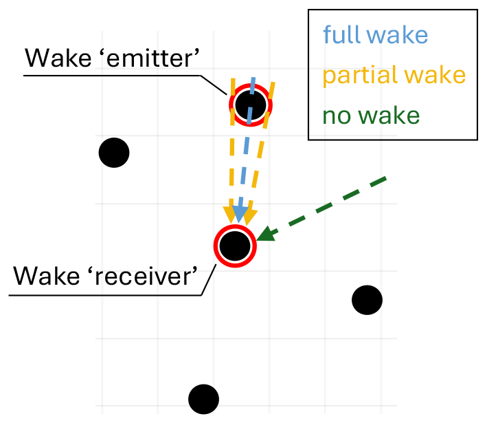
Figure 3 Simulated wind farm with highlighted locations of two turbines of interest and selected wind directions for the training process.

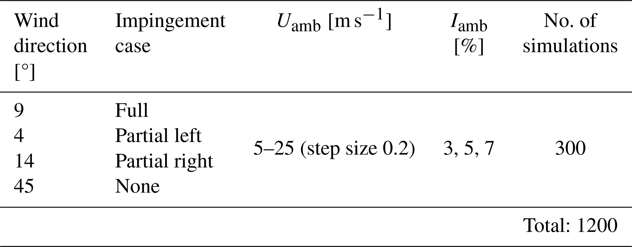
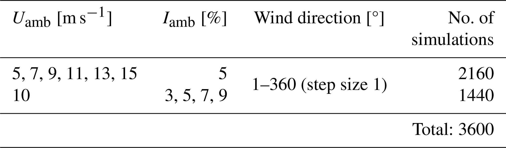
A dataset comprised of 1200 simulations is produced, with simulation parameters and run counts presented in Table 1. Ambient wind speed U_amb and ambient turbulence intensity I_amb values are varied to ensure that the simulated conditions represent a multitude of different offshore wind states. Each simulation consists of generating a unique wind field and calculating the corresponding time series of instantaneous turbine response. Synthetic wind fields are acquired by generating ambient turbulence boxes using the Mann spectral tensor model (Mann, 1994) and superimposing them with wakes generated with the SGRE's in-house implementation of the DWM model (Larsen et al., 2007). The version of the model used follows the parameterisation suggested in the latest IEC standard (IEC, 2019). In its essence, the DWM model regards the wake as a passive tracer being moved laterally and vertically by stochastic turbulence with a characteristic length of twice the rotor diameter or larger. The turbine operation for the simulated conditions is calculated using the aeroelastic code BHawC. Since ambient wind fields are acquired with the Mann turbulence model, the atmospheric conditions are assumed to be neutral (Mann, 1994). The presence of vertical wind shear is simulated using the wind profile power law, with a shear exponent value of 0.07 selected for all cases. Turbines are simulated with no yaw angle misalignment.

Table 1 Training simulation subsets. For each wind direction, 300 simulations capturing all U_amb and I_amb combinations are performed.

2.3 Framework implementation: wind sensing

2.3.1 Wind sensing input and output data selection

Figure 4 illustrates the training of the wind sensing model and demonstrates its application scheme. By providing a varied dataset of turbine response time series and the corresponding wind field representations, the estimator “learns” to approximate the wind speed distribution at the rotor from the turbine sensor data.

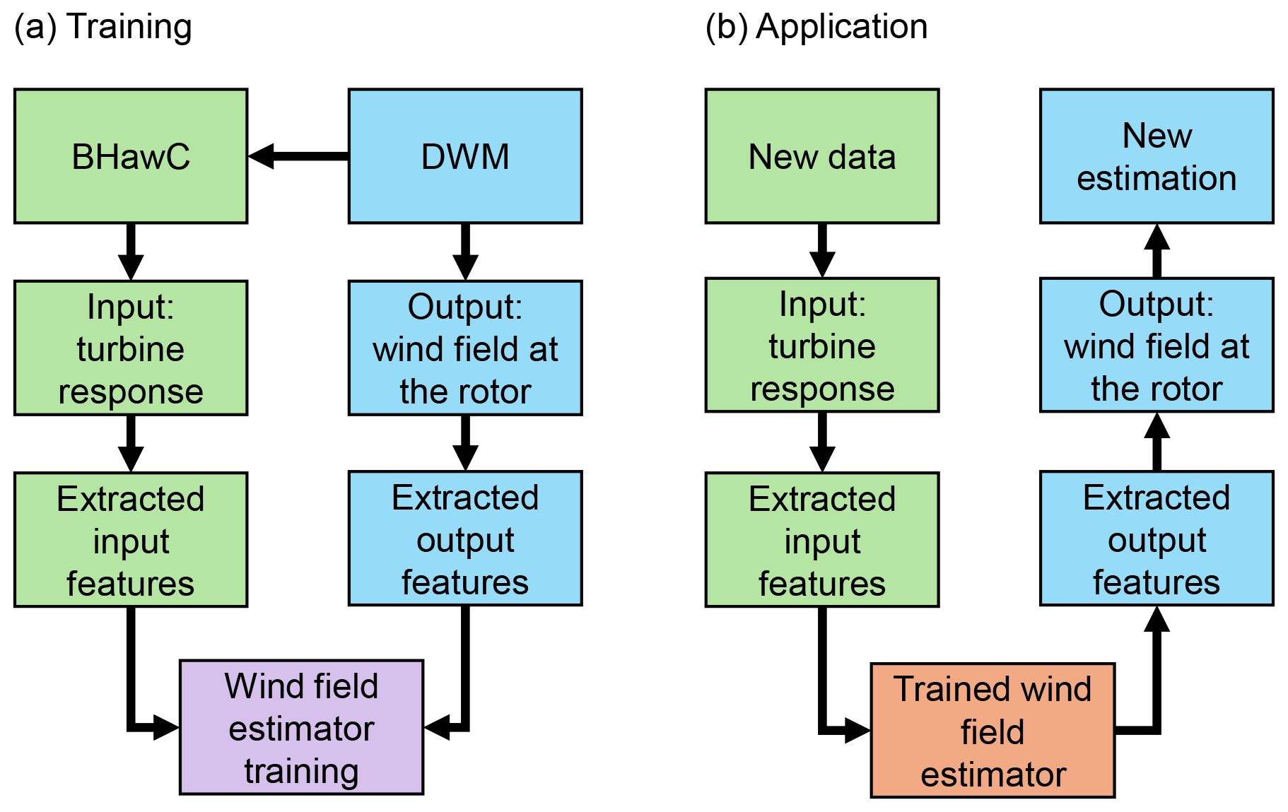
Figure 4 Simplified diagram visualising the flow of data during (a) training and (b) application of the wind sensing model.

The aeroelastic code provides access to an extensive set of turbine response signals, such as component accelerations or generator speed. A conditional dependence analysis (readers further interested in the specific method used are referred to Azadkia and Chatterjee, 2021) is undertaken to determine which data channels are best coupled with the variations in the flow. The algorithm tests different combinations of turbine signals, estimating the likelihood that wind speed can be deterministically predicted from them. The following combination with the strongest overall correlation to wind speed is identified and used in wind sensing: blade root bending moments in both the flap-wise and the edge-wise directions; mean pitch across all three blades, simply calculated as $\stackrel{\mathrm{‾}}{\mathit{\beta }}=({\mathit{\beta }}_{\mathrm{1}}+{\mathit{\beta }}_{\mathrm{2}}+{\mathit{\beta }}_{\mathrm{3}})/\mathrm{3}$; and rotor rotational speed ω. Rotor azimuth angle and individual pitch angles are also extracted to use for transformations of other inputs.

The wind field is considered to be a three-dimensional Cartesian grid, with three axes: X, representing streamwise distance; Y, representing lateral distance; and Z, representing vertical distance. To represent the wind speed distribution in the flow, each point on that grid stores the local values of three wind speed components, U, V and W, which correspond to the spatial variation in the X, Y and Z axes, respectively. For this specific application, the wind field is represented with the spatial distribution of the longitudinal wind speed component U, as it is the one that is primarily impacted by wake deficit (Dimitrov et al., 2017). All models treat the wind field as a time series of YZ slices, showing the chronological sequence of U distributions at the rotor plane.

2.3.2 Wind sensing input processing

Selected turbine response time series are processed to extract the optimal features from the raw data. The processes described in this section are applied during both training and performance testing – they are an integral part of the data “pipeline”. Figure 5 illustrates the transformations taking place in the feature extraction.

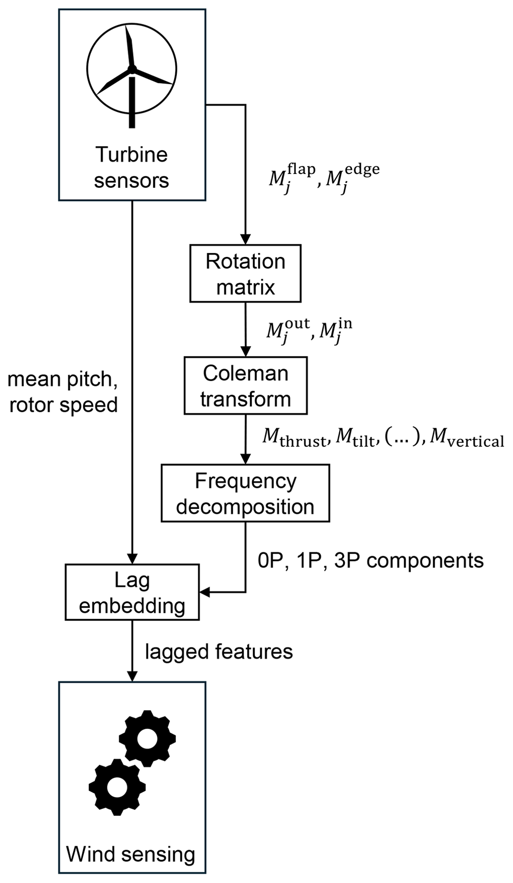
Figure 5 Block diagram of the turbine response processing. $M_j^{\mathrm{flap}/\mathrm{edge}}$ – flap/edge blade root bending moments, $M_j^{\mathrm{out}/\mathrm{in}}$ – in- and out-of-plane blade root bending moments, j – blade index, $M_{\mathrm{thrust}/\mathrm{tilt}/\left(\mathrm{\dots }\right)/\mathrm{vertical}}$ – rotor loads. A detailed description can be found in the text.

First, using the pitch signals, the edge- and flap-wise blade root bending moments are transformed to in- and out-of-plane coordinates. Performing the rotation between the two frames is calculated for a given blade j as follows:

$$\begin{array}{}\text{(1)}& \left[\begin{array}{c}{M}_j^{\mathrm{out}}\\ M_j^{\mathrm{in}}\end{array}\right]=\left[\begin{array}{cc}\cos \left({\mathit{\beta }}_j\right)& \sin \left({\mathit{\beta }}_j\right)\\ -\sin \left({\mathit{\beta }}_j\right)& \cos \left({\mathit{\beta }}_j\right)\end{array}\right]\left[\begin{array}{c}{M}_j^{\mathrm{flap}}\\ M_j^{\mathrm{edge}}\end{array}\right],\end{array}$$

where $M_j^{\mathrm{out}}$ and $M_j^{\mathrm{in}}$ are out-of- and in-plane root bending moments, respectively; $M_j^{\mathrm{flap}}$ and $M_j^{\mathrm{edge}}$ are flap and edge root bending moments, respectively; and β_j is the instantaneous pitch angle.

Next, using the azimuth angle time series, the Coleman transformation (Coleman, 1943) is applied to the blade load data. It allows us to effectively map the separate, rotary-frame bending moments from each blade onto a stationary frame of reference. As a result, the dynamic response to the variation in the wind can be expressed with six variables describing the loads for an entire rotor: M_thrust, M_tilt and M_yaw (for out-of-rotor-plane movement) and M_torque, M_lateral and M_vertical (for in-rotor-plane movement). These are referred to as rotor loads. The Coleman transformation is defined as follows:

$$\begin{array}{}\text{(2)}& \begin{array}{rl}\mathbf{C}\left(\mathit{\psi }\right)=& \left[\begin{array}{ccc}\mathrm{1}/\mathrm{3}& \mathrm{0}& \mathrm{0}\\ \mathrm{0}& \mathrm{2}/\mathrm{3}& \mathrm{0}\\ \mathrm{0}& \mathrm{0}& \mathrm{2}/\mathrm{3}\end{array}\right]\cdot \\ & \left[\begin{array}{ccc}\mathrm{1}& \mathrm{1}& \mathrm{1}\\ \cos \left(\mathit{\psi }\right)& \cos \left(\mathit{\psi }+\frac{\mathrm{2}\mathit{\pi }}{\mathrm{3}}\right)& \cos \left(\mathit{\psi }+\frac{\mathrm{4}\mathit{\pi }}{\mathrm{3}}\right)\\ \sin \left(\mathit{\psi }\right)& \sin \left(\mathit{\psi }+\frac{\mathrm{2}\mathit{\pi }}{\mathrm{3}}\right)& \sin \left(\mathit{\psi }+\frac{\mathrm{4}\mathit{\pi }}{\mathrm{3}}\right)\end{array}\right],\end{array}\end{array}$$

where ψ is the rotor azimuth angle. It is used to transform the blade loads as follows:

$$\begin{array}{}\text{(3)}& {\displaystyle }& {\displaystyle }\left[\begin{array}{c}{M}_{\mathrm{thrust}}\\ M_{\mathrm{tilt}}\\ M_{\mathrm{yaw}}\end{array}\right]=\mathbf{C}\left(\mathit{\psi }\right)\left[\begin{array}{c}{M}_{\mathrm{1}}^{\mathrm{out}}\\ M_{\mathrm{2}}^{\mathrm{out}}\\ M_{\mathrm{3}}^{\mathrm{out}}\end{array}\right],\text{(4)}& {\displaystyle }& {\displaystyle }\left[\begin{array}{c}{M}_{\mathrm{torque}}\\ M_{\mathrm{lateral}}\\ M_{\mathrm{vertical}}\end{array}\right]\mathbf{C}\left(\mathit{\psi }\right)\left[\begin{array}{c}{M}_{\mathrm{1}}^{\mathrm{in}}\\ M_{\mathrm{2}}^{\mathrm{in}}\\ M_{\mathrm{3}}^{\mathrm{in}}\end{array}\right],\end{array}$$

where $M_{\mathrm{1}\text{–}\mathrm{3}}^{\mathrm{out}}$ is the out-of-plane bending moment, and $M_{\mathrm{1}\text{–}\mathrm{3}}^{\mathrm{in}}$ is the in-plane bending moment for blade indices 1–3.

The rotor load time series are decomposed into their key frequency components. This process is visualised in Fig. 6. The five frequency components selected via a conditional dependence study (Azadkia and Chatterjee, 2021) are cos(0P), used to describe the mean signal value; cos(1P) and sin(1P), used to describe the once-per-revolution variation; and, finally, cos(3P) and sin(3P), used to describe the thrice-per-revolution variation. A sliding window function with a width of three revolutions is applied, projecting the original load time series onto each of the frequency components. The Fourier coefficient vectors (a₁–a₅) obtained from these projections are stored, producing a coefficient time series for each rotor load.

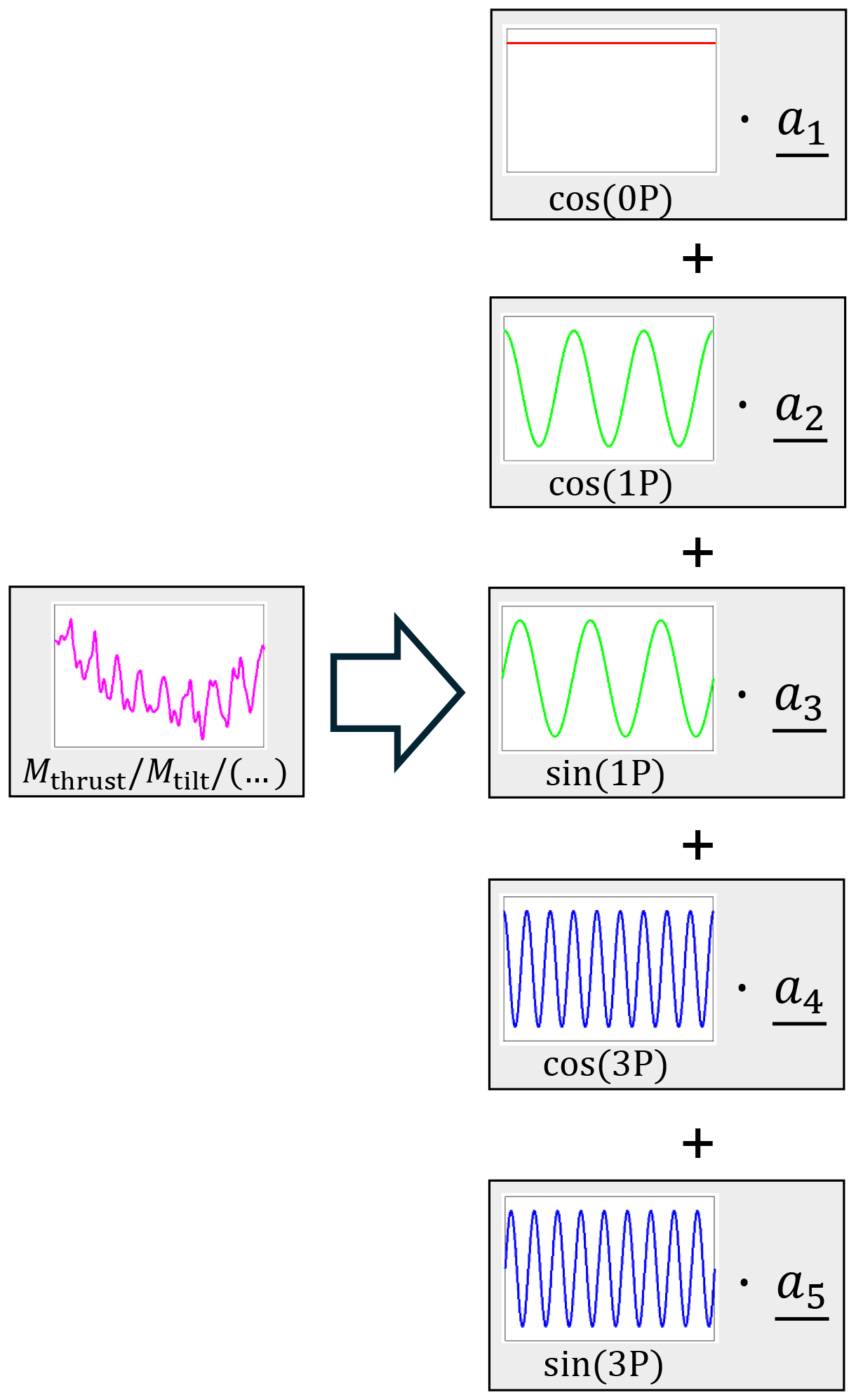
Figure 6 An example of rotor load time series decomposition into frequency component coefficient vectors (a₁–a₅), capturing the contributions of each Fourier mode at each point in time.

In order to capture the short-term temporal dependencies and patterns in the time series of all wind sensing inputs, the features are embedded with their lagged values. For each sample in a time series, two additional features expressing the past value of the curve are added. These lagged features are obtained by shifting the time series 4 and 8 s from the current time stamp. This effectively makes the estimation more stable and noise resistant, as the wind slice is reconstructed with turbine response across several seconds. Specific lag values used are determined by testing the framework's performance with a few different configurations and choosing the one that gives the best overall results.

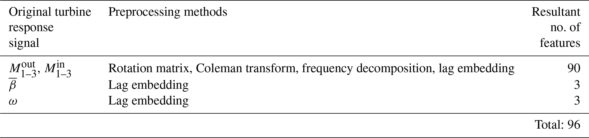
Due to implementing the transformations discussed in this section, using the turbine response data as wind sensing input effectively stops being a time series modelling task; instead, it becomes a time-independent regression task. Considering the entire feature extraction process, at each point in time, a 96-dimensional input vector captures and encodes the turbine's current operating state. Table 2 serves as a summary of these features.

Table 2 A summary of features extracted from turbine response.

2.3.3 Wind sensing output processing

The three-dimensional wind field representations are processed for data compression and efficient extraction of their key features for the best application in wind sensing. The wind field is represented with a sequence of YZ slices showing the U distribution at each point along the X axis. The spatial features of each slice are extracted, capturing the key characteristics of the wind field in a more compact form. The feature extraction is performed using the two-dimensional discrete cosine transform (DCT) (Ahmed et al., 1974). The result is similar to applying the principal component analysis; however, as opposed to this far more complex method, the DCT is a fixed transform and does not require any training. The DCT effectively converts the wind slice into a collection of cosine functions oscillating at different frequencies in both the vertical and the horizontal directions. Each DCT coefficient corresponds to a specific frequency in the transformed domain and describes the contribution of each frequency in the distribution of U on the given YZ slice. This concept, applied to an example wind field YZ slice, is presented in Fig. 7.

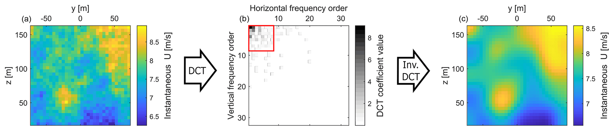
Figure 7 An example showing how the YZ slice of the wind field (a) is transformed into a matrix of DCT components (b) and then back into a truncated slice of wind through an inverse DCT (c). The red square indicates which DCT coefficients are stored for the implemented wind field representation.

The lower-order frequencies primarily capture the large-scale structures of the field, while the higher-order frequencies are more associated with encoding smaller-scale, random fluctuations. It can be seen that the most significant values can be found in the upper-left corner of the diagram, meaning the majority of flow distribution is being kept by the lower orders of DCT coefficients. For this reason, the key information on the flow can be easily extracted by storing only the lower-order coefficients and disregarding the higher-order coefficients. Truncating the collection of DCT-order coefficients essentially acts as a spatial low-pass filter. In this work, retention of eight DCT coefficients is found to enhance computational efficiencies while allowing for good wind sensing accuracy. The right plot in Fig. 7 shows the effect of truncating the higher frequencies; it can be noticed how the wind slice is significantly “smoothed”, leaving only the major U fluctuations.

2.3.4 Training the wind sensing estimator

Having extracted the features from both the inputs and the outputs, two-thirds of data are used for the wind field estimator training, while the remaining one-third is put aside for generating wind field estimations for wake detector testing. The current implementation utilises a localised linear regression approach (Cleveland et al., 1988), where the estimator training is performed for multiple localised models. The preprocessed turbine response data are a time series of multidimensional input points, with each dimension representing a different feature (see Table 2). Two of these dimensions, namely unlagged $\stackrel{\mathrm{‾}}{\mathit{\beta }}$ and unlagged ω (these being the key variables indicating the turbine's operating point), are used to define a projection plane, allowing input points to be mapped and binned by their values. A set of evenly spaced points on this plane is selected, and a local linear regression model is trained at each. Training data are assigned to models based on proximity within a defined radius, with overlapping points contributing to multiple estimators. Predictions for new inputs are made using the model nearest to their location on the projection plane. As a result, the training process builds functions that correlate the inputs to outputs only at a narrow section of data distribution. This eliminates the need to fit a global non-linear function that would singlehandedly need to describe the complex relationship between wind and turbine signals.

2.4 Framework implementation: wake detection

Considering that wake detection can essentially be reduced to a classification task, we propose dealing with it by implementing a convolutional neural network. The overview of this deep learning technique can be found in Appendix A. The approach is to operate on the YZ snapshot samples (so-called “front view”), which show the estimated instantaneous wind component U across the whole rotor area. This allows for clear differentiation between impinged and non-impinged conditions. To accurately capture the different forms of wake impingement, four distinct classes are defined. These are as follows: (a) fully impinged, with the turbine directly downstream of the closest neighbour; (b) partially impinged left, with the wake impacting the left side of the rotor; (c) partially impinged right, with the wake impacting the right side of the rotor; and (d) no detectable impingement.

The turbine response time series from the remaining 400 simulations, set aside during the wind sensing estimator training, are now used for generating wind field estimations. These estimations form the basis of a new dataset for CNN training. The training samples are labelled according to the wind direction specified in their respective simulation setup. In turn, the four classes directly relate to the four wind directions used during the training data acquisition (see Sect. 2.2). An extensive manual review of the produced samples allows for the following conclusion: in the available dataset, a clear, non-dissipated wake is only visible for lower values of the selected ambient wind speed range – typically up to 14–16 m s⁻¹, depending on the ambient turbulence intensity. Simulations with higher wind speeds exhibit stronger wake meandering, which results in the wake deficit often being absent from the YZ snapshot samples. The wake deficit depth is also weaker due to the smaller thrust force in the above-rated operation. Consequently, many samples labelled “fully” or “partially impinged” do not, in fact, exhibit a wake. The aim of the detector is to reliably recognise whether the turbine is likely experiencing a wake impingement from a nearby machine. To ensure this robustness, the training data must exclude the aforementioned mislabelled samples. With that in mind, the CNN is trained with data from simulations where the mean ambient wind speed U_amb is between 5 and 15 m s⁻¹ while maintaining the full range of turbulence intensity values (3 %, 5 % and 7 %). The YZ snapshot samples are taken every 10 s from the available training data, resulting in 11 200 labelled samples. Figure 8 shows selected YZ samples being appropriate examples of each one of the four classes.

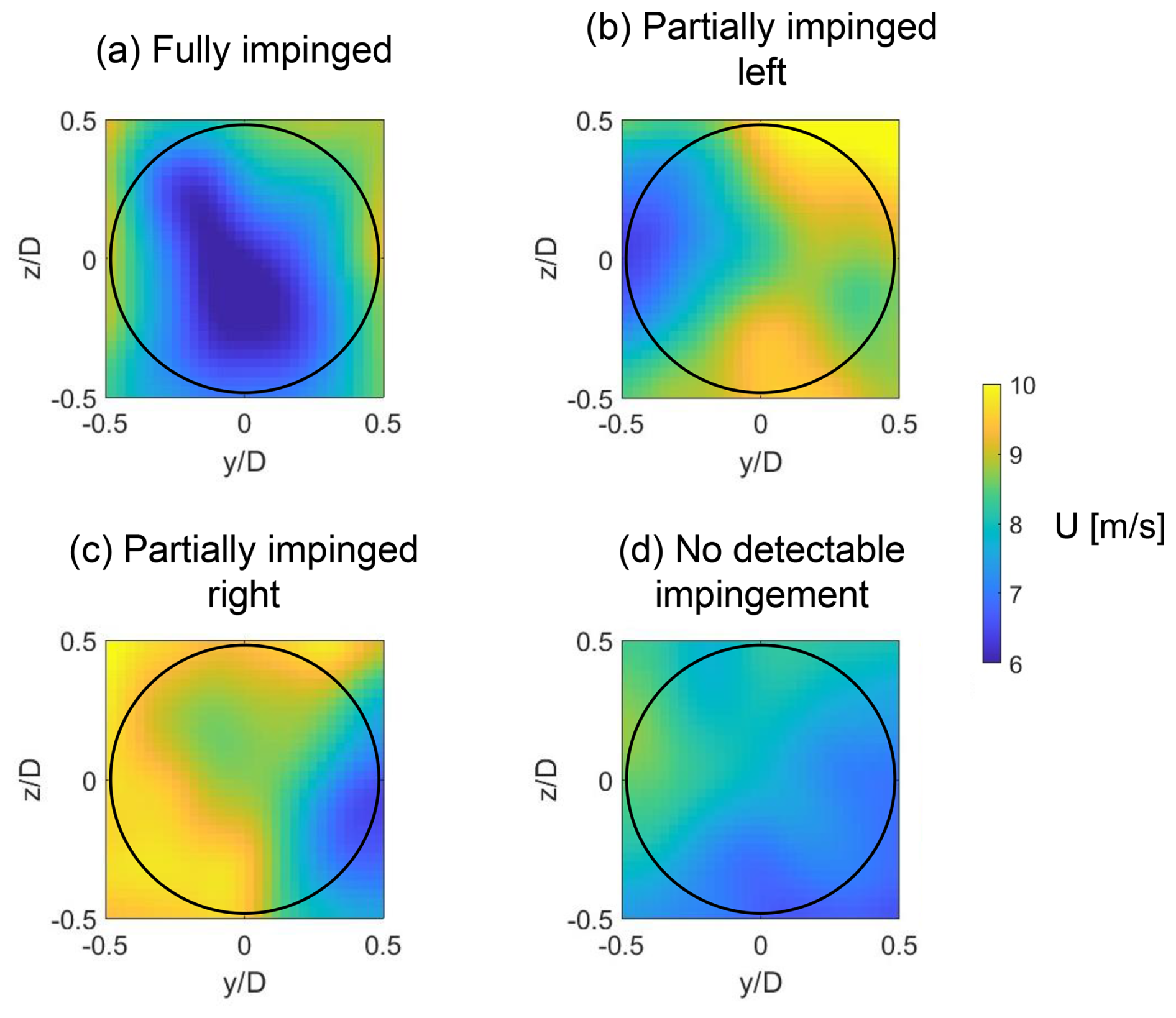
Figure 8 Example front-view YZ snapshot samples representing four classes defined for the neural network training. The rotor area is indicated with the black circle.

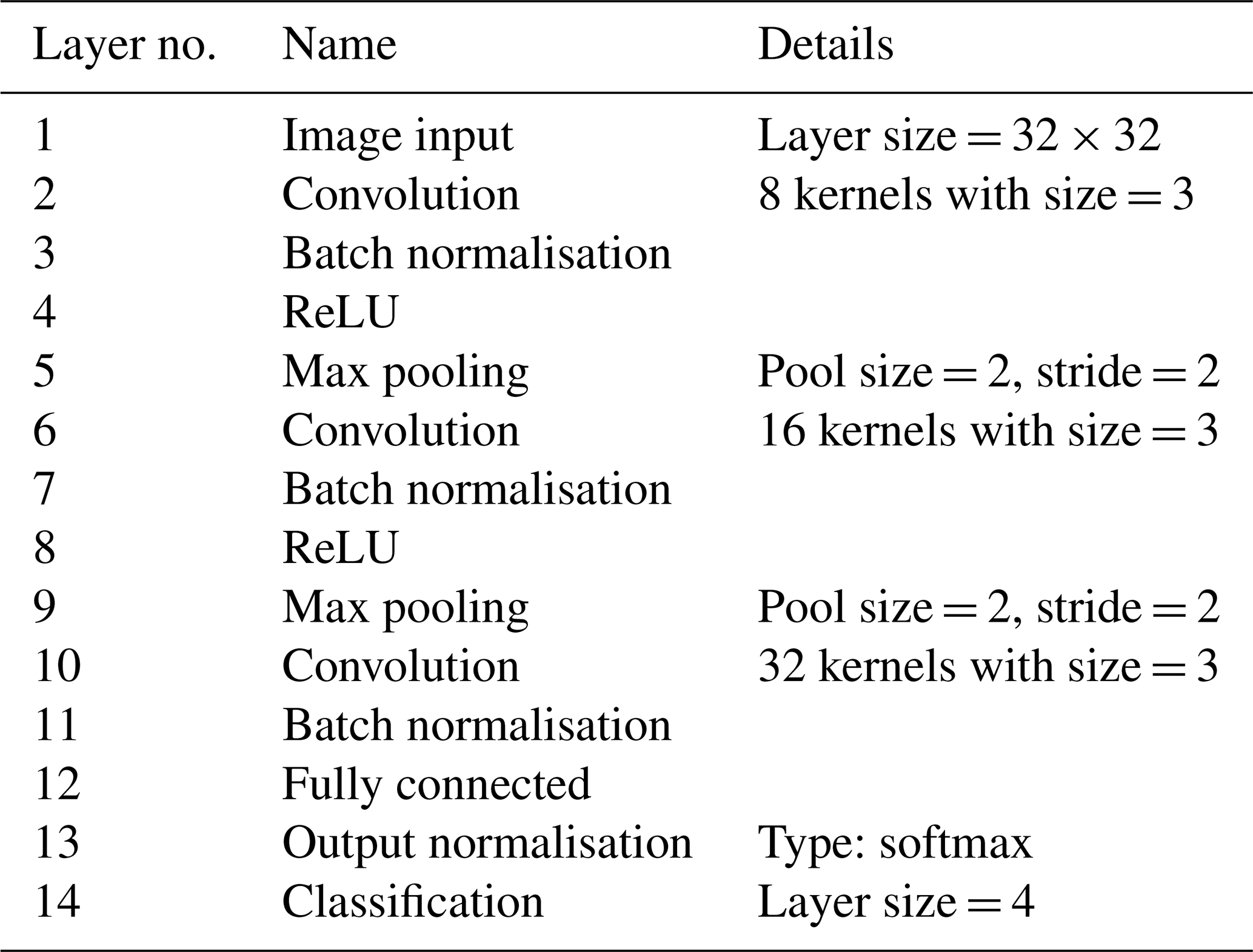
The implemented CNN architecture is presented in Table 3. The input layer has the same resolution as the YZ slice of estimated wind. The three convolution layers have an increasing number of kernels, allowing the network to progressively learn more complex features at deeper levels (Goodfellow et al., 2016). A batch normalisation layer is added after each of the convolution layers for the sake of normalisation of weight gradients and neuron activations, thus speeding up the training process. Two max pooling layers reduce the spatial size of the feature maps. The activation function is selected as the rectified linear unit (ReLU). The final three layers transform the learned features into predictions, connecting all of the neurons, normalising outputs into probabilities and performing final classification. An extended description of the layers used can be found in Appendix A. The optimal hyperparameter values are chosen based on trial and error, with the CNN accuracy monitored through integrated testing.

Table 3 Implemented CNN architecture.

The training is conducted using MATLAB's Deep Learning Toolbox. A total of 90 % of the available labelled data (10 080 samples) are used for training. The samples are shuffled before the training process and after each one of the four epochs. The training is repeated several times to make sure there are no deviations. The remaining 10 % of samples are used for an integrated testing cycle, which automatically occurs after the training is complete. Figure 9 shows its results in the form of a confusion matrix. As can be observed, the main source of error is the misclassifications between the “fully impinged” and “no detectable impingement” classes. This phenomenon is further investigated in Sects. 3 and 4, where the performance of each of the models is analysed in more detail under a variety of conditions.

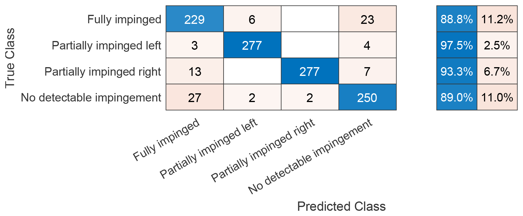
Figure 9 Confusion matrix for the integrated testing of the trained CNN. Each row represents the instances of a true class, whereas each column represents the instances of a predicted class. As a result, the values in the diagonal (blue) and off-diagonal (orange) cells correspond to correct and false classifications, respectively. Percentages of correct (blue) and false (orange) classifications within each true class are shown on the right.

2.5 Framework implementation: wake characterisation

The final part of the developed framework is the identification of the key wake parameters in cases where a clear wake impingement is detected. This is undertaken by scanning for the characteristic velocity deficit shape in the appropriate wind field representations.

2.5.1 Two-dimensional Gaussian fitting

The “tracking” of wake position and width is achieved by implementing a two-dimensional Gaussian fitting scheme based on a least squares algorithm. This method is a commonly used solution in the literature for dynamic wake property analysis (Abkar and Porté-Agel, 2015; Trujillo et al., 2011; Conti et al., 2020). First, the wake deficit is defined for every sample as follows:

$$\begin{array}{}\text{(5)}& U_{\mathrm{def}}(y,z)=U(y,z)-U_{\mathrm{amb}},\end{array}$$

where U(y,z) is the instantaneous wind speed distribution across the YZ plane, and U_amb is the mean ambient wind speed value.

A general bivariate two-dimensional Gaussian function for spatial variables of y and z is expressed as

$$\begin{array}{}\text{(6)}& \begin{array}{rl}{f}_{\mathrm{bivariate}}(y,z)& ={\displaystyle \frac{A}{\mathrm{2}\mathit{\pi }{\mathit{\sigma }}_y{\mathit{\sigma }}_z\sqrt{\mathrm{1}-{\mathit{\rho }}^{\mathrm{2}}}}}\exp \left[-{\displaystyle \frac{\mathrm{1}}{\mathrm{2}\left(\mathrm{1}-{\mathit{\rho }}^{\mathrm{2}}\right)}}\right.\\ & \left({\displaystyle \frac{{\left(y-y_{\mathrm{c}}\right)}^{\mathrm{2}}}{{\mathit{\sigma }}_y^{\mathrm{2}}}}-{\displaystyle \frac{\mathrm{2}\mathit{\rho }\left(y-y_{\mathrm{c}}\right)\left(z-z_{\mathrm{c}}\right)}{{\mathit{\sigma }}_y{\mathit{\sigma }}_z}}\right.\\ & \left.\left.+{\displaystyle \frac{{\left(z-z_{\mathrm{c}}\right)}^{\mathrm{2}}}{{\mathit{\sigma }}_z^{\mathrm{2}}}}\right)\right],\end{array}\end{array}$$

where A is the amplitude equal to the height of the peak; σ_y and σ_z are standard variations along the Y and Z axes, respectively; ρ is the correlation coefficient between the function's spread in Y and Z; and y_c and z_c are the means along Y and Z, respectively.

The time series of wake deficits from Eq. (5) is fitted to Eq. (6) through a Levenberg–Marquardt non-linear least squares algorithm implemented with MATLAB's Optimization Toolbox. Fitted Gaussian parameters are then used to identify wake properties: the function peak at (y_c, z_c) can be interpreted as the position of the wake centre; σ_y and σ_z describe the spread of the wake along the Y and Z axes, respectively; and ρ can be used to calculate the lengths of the semi-minor and semi-major axes of the wake ellipse and their orientation with respect to the YZ axes. The initial guess for σ_y and σ_z is defined as half of the rotor diameter D in order to best reflect the typical width expected of a wake.

As explained earlier, the framework outputs refer solely to the lateral wake characteristics, which are expressed by the variation on the Y axis. Out of all fitted parameters, only two are required to describe the lateral wake variation: y_c and σ_y. To parametrically represent the size of the wake deficit, it is assumed that the lateral half width corresponds to the standard deviation in the Y direction. With that in mind, the wake extends laterally for 2σ_y, with the fitted centre y_c in the middle. Figure 10 shows an example of the bivariate two-dimensional Gaussian fit applied on a YZ wind field sample, with the key characterised properties indicated.

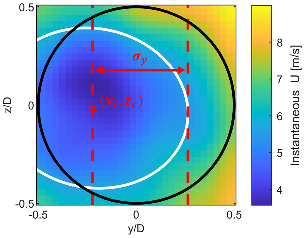
Figure 10 An example of a bivariate two-dimensional Gaussian fit performance applied to a YZ wind field sample. The rotor outline is marked with the black line, the fitted wake ellipse is marked with the white line, the fitted wake centre at (y_c, z_c) is marked with the red x sign and the extent of the fitted lateral half width σ_y is marked with dashed lines.

2.5.2 Filtering with moving average window

The lateral wake half-width and centre position time series are smoothed using a moving average filter to reduce high-frequency noise from sample-by-sample variability while preserving slower variations associated with wake meandering. This way, the ultimate characterised wake property time series $y_{\mathrm{c}}^{\mathrm{filt}}$ and ${\mathit{\sigma }}_y^{\mathrm{filt}}$ are defined as follows:

$$\begin{array}{}\text{(7)}& \left[\begin{array}{c}{y}_{\mathrm{c}}^{\mathrm{filt}}\left(t\right)\\ {\mathit{\sigma }}_y^{\mathrm{filt}}\left(t\right)\end{array}\right]={\displaystyle \frac{\mathrm{1}}{\mathit{\tau }}}\underset{t-\mathit{\tau }}{\overset{t}{\int }}\left[\begin{array}{c}{y}_{\mathrm{c}}\left(\mathit{\theta }\right)\\ {\mathit{\sigma }}_y\left(\mathit{\theta }\right)\end{array}\right]\mathrm{d}\mathit{\theta }.\end{array}$$

The variable τ stands for window size in seconds, which is calculated separately for every wind field in the following manner:

$$\begin{array}{}\text{(8)}& \mathit{\tau }={\displaystyle \frac{L_{\mathrm{meand}}}{\stackrel{\mathrm{‾}}{U_{\mathrm{hh}}}}},\end{array}$$

where L_meand is the characteristic meandering length equal to two rotor diameters (with the value corresponding to findings from the literature, used in several wake models like the DWM itself, Larsen et al., 2007), and $\stackrel{\mathrm{‾}}{U_{\mathrm{hh}}}$ is the mean U value at hub height.

It should be noted that in this method of moving average filtering, the averaging window is not centred at the current sample; instead, the window extends from the past sample occurring τ seconds ago to the current sample. As a result, the filtered wake centre and lateral half-width time series experience a small lag of $\mathit{\tau }/\mathrm{2}$.

2.5.3 Treatment of non-impinged samples

To satisfy the assumption that wake characterisation should not be performed for wind samples without clear impingement, the filtered wake properties are treated for a given time stamp i as follows:

$$\begin{array}{}\text{(9)}& \begin{array}{rl}& y_{\mathrm{c}}^{\mathrm{filt}}\left(i\right),{\mathit{\sigma }}_y^{\mathrm{filt}}\left(i\right)=\\ & \left\{\begin{array}{ll}{y}_{\mathrm{c}}^{\mathrm{filt}}\left(i\right),{\mathit{\sigma }}_y^{\mathrm{filt}}\left(i\right),& \mathrm{if}\mathrm{class}\left(i\right)=\mathrm{fully}/\mathrm{partially}\mathrm{impinged}\\ \mathrm{NaN},& \mathrm{if}\mathrm{class}\left(i\right)=\mathrm{no}\mathrm{detectable}\mathrm{impingement}\end{array}\right..\end{array}\end{array}$$

The assignment of NaN (not a number) values ensures that the samples identified as non-impinged are not being represented with a two-dimensional Gaussian wake in the framework output.

3 Results

3.1 Performance evaluation

The framework's performance is evaluated with 3600 new simulations divided into 10 subsets. The configurations with the number of runs are shown in Table 4. Each simulation is paired with the corresponding turbine response. All simulations are performed for one “receiver” turbine, which is more centrally located within the wind farm compared to the machine used for the training; by doing so, it experiences different types of impingement for different wind directions. Both qualitative and quantitative performance analysis is conducted for each of the three constituent models.

Table 4 Testing simulation subsets. For each U_amb and I_amb combination, 360 simulations capturing the full wind direction spectrum are performed.

In this work, the reference for quantitative analysis of the models' accuracy is the collection of the raw DWM-generated wind fields. Wind sensing accuracy analysis is a straightforward calculation of root mean square error (RMSE) between the U data points in simulated wind fields and the estimated equivalents. A reference for wake detection accuracy analysis is created via a new classifier trained analogically to the process described in Sect. 2.4, with the only difference being that the training dataset is derived from simulated wind fields, not the estimated ones. Without the bias from the wind field reconstruction, this classifier achieves approximately 99 % accuracy under integrated testing. As such, its classifications across all 3600 raw wind fields (with the wind sensing step not performed) are thus taken to be the “ground truth” reference. Finally, the reference for wake characterisation is obtained by processing a raw simulated wind field: a two-dimensional Gaussian is fitted, moving average filtering is applied and “non-impinged” wind slice samples are removed analogically to the process described in Sect. 2.5.

The wind sensing accuracy is first analysed by plotting the RMSE across the YZ plane for two example simulations from the testing dataset, presenting low and high ambient turbulence. This is shown in Sect. 3.2. The wind-direction-dependent wind sensing and wake detection performance is then analysed via a study of the sensitivity to U_amb and I_amb, comparing these models' mean accuracy across the entirety of the 10 subsets described above. This is discussed in Sect. 3.3. Section 3.4 presents detailed wake characterisation results. This is achieved by visualising the framework's performance across selected wind fields from the testing dataset, followed by computing the quantitative performance metrics of wake characterisation.

3.2 Wind sensing: YZ-wise accuracy

Figure 11 compares the YZ plane distribution of the wind sensing RMSE for low (a) and high (b) turbulence intensity. This distribution is obtained by calculating RMSE_sen at every YZ location over the full duration of the simulation n_t:

$$\begin{array}{}\text{(10)}& {\mathrm{RMSE}}_{\mathrm{sen}}(y,z)=\sqrt{{\displaystyle \frac{\mathrm{1}}{n_t}}\sum _{i=\mathrm{0}}^{n_t}\left(U_i^{\mathrm{est}}\right(y,z)-U_i^{\mathrm{DWM}}(y,z){)}^{\mathrm{2}}},\end{array}$$

where $U_i^{\mathrm{est}}(y,z)$ and $U_i^{\mathrm{DWM}}(y,z)$ are the YZ-specific U at time i for the estimated and DWM wind field, respectively. Both plots show the error to be higher at the rotor centre and in the corners outside the rotor area. The high-I_amb plot reports significantly higher RMSE, with the critical corner area reaching approximately twice the value of the low-turbulence case. The ring-like pattern of the area with the lowest error (dark blue in the plot) is repeated across all wind conditions, whose plots are not shown here for brevity.

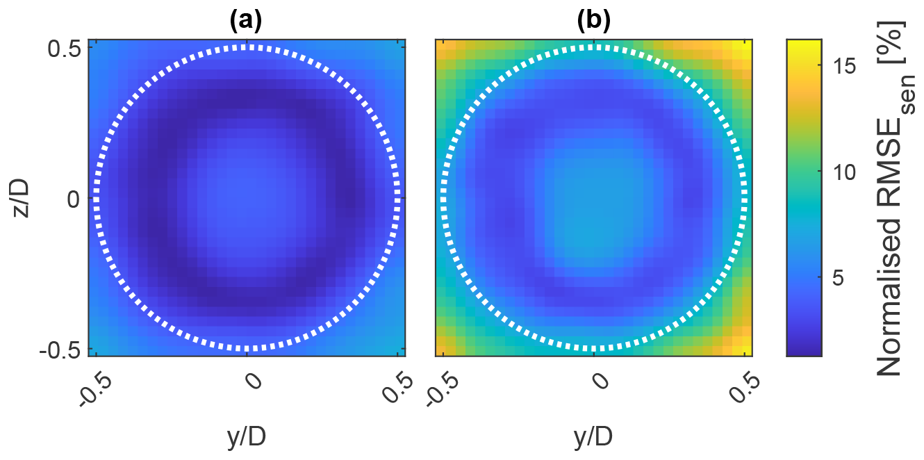
Figure 11 Wind sensing RMSE plotted across YZ slice, normalised by the corresponding U_amb value of 10 m s⁻¹. (a) I_amb=3 %; (b) I_amb=9 %. The rotor outline is marked with the dotted white line.

3.3 Wind sensing and wake detection: ambient condition sensitivity study

For all 3600 simulations, the YZ distributions of wind sensing RMSE (such as the examples in Fig. 11) are averaged across the entire rotor plane to obtain a single simulation-specific mean value. Furthermore, to check how the RMSE changes with wind conditions, mean $\stackrel{\mathrm{‾}}{{\mathrm{RMSE}}_{\mathrm{sen}}}$ values averaging all 360 simulations with the same U_amb and I_amb are calculated. These values are presented in Table 5.

Table 5 A comparison of performance metrics in wind sensing and wake detection under varying U_amb and I_amb. $\stackrel{\mathrm{‾}}{{\mathrm{RMSE}}_{\mathrm{sen}}}$ is normalised by the corresponding U_amb value.

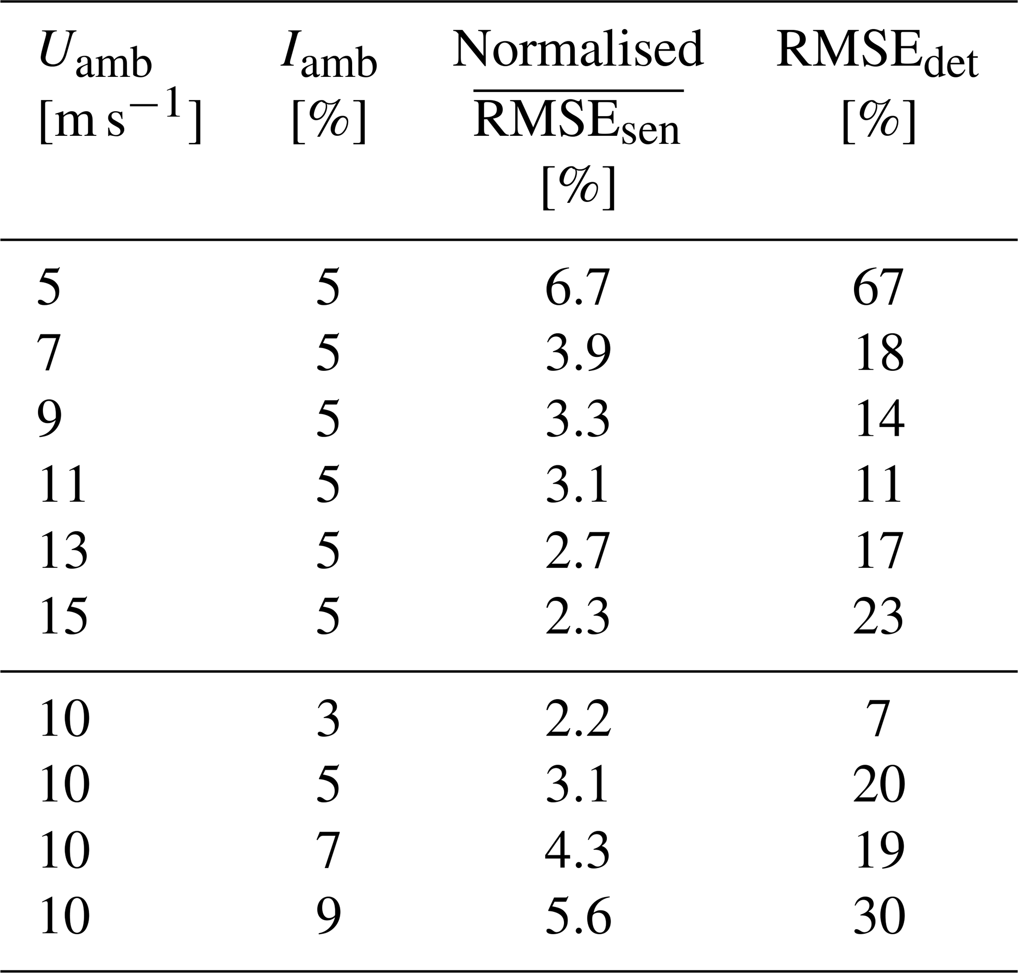
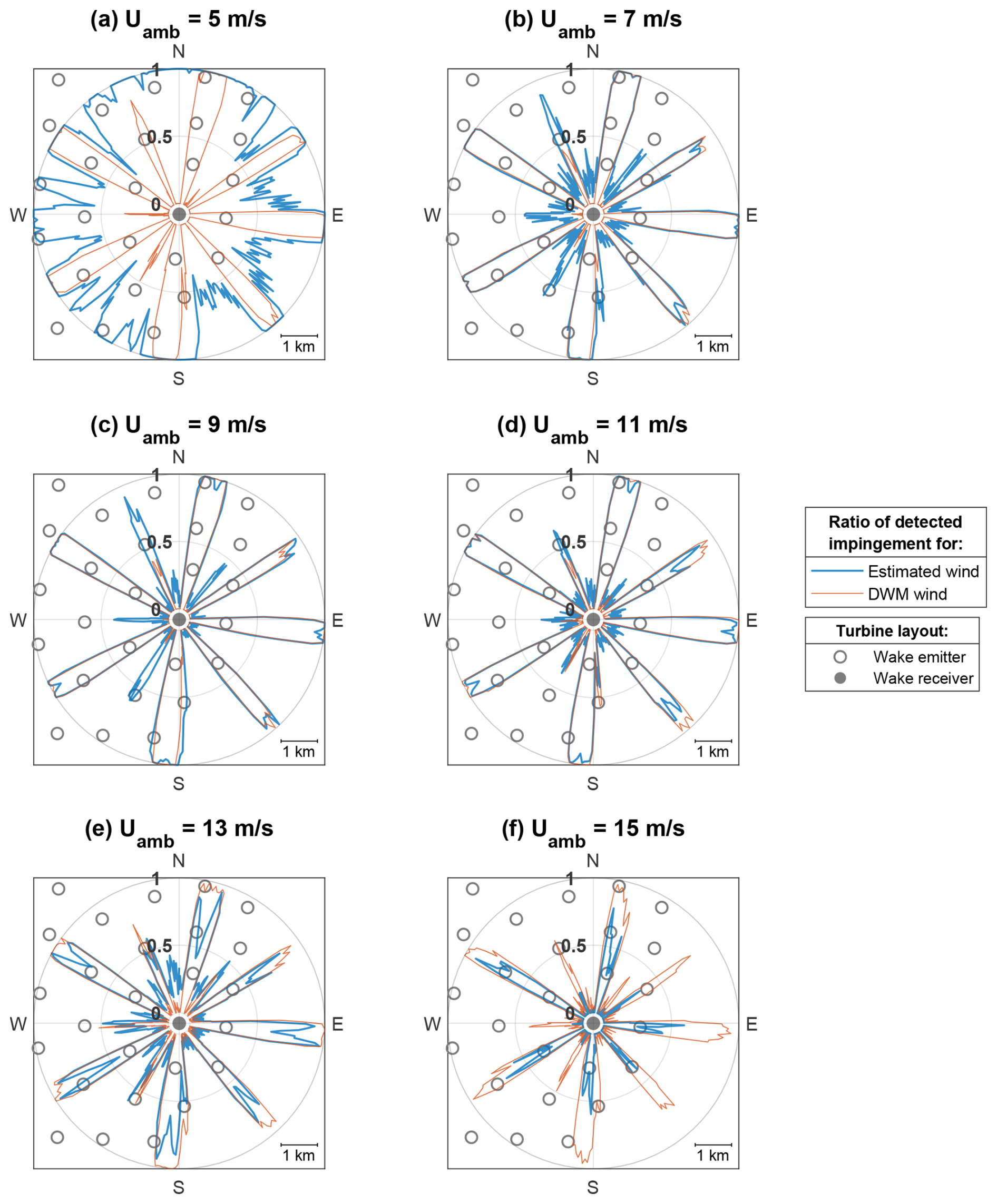
Figure 12 The wake detection model performance tested under a full wind direction range for six U_amb values between 5 and 15 m s⁻¹. I_amb=5 % for all cases. The radial values in blue and orange indicate the impingement ratio for a given wind direction. The wind farm layout is shown in the background.

For each of the 3600 simulations, the proportion of samples (YZ wind slices at a point in time) classified as a clear wake impingement (“fully impinged”, “partially impinged left” or “partially impinged right”) is calculated. These simulation-specific impingement ratios are compared to their equivalents in the reference established by the “ground truth” classifier (see Sect. 3.1). This provides a quantitative measure of the wake detection error for a given wind direction. A single wake detection RMSE_det value is calculated across the entire wind direction range for each of the 10 U_amb and I_amb combinations:

$$\begin{array}{}\text{(11)}& {\mathrm{RMSE}}_{\det }=\sqrt{{\displaystyle \frac{\mathrm{1}}{n_{\mathrm{wd}}}}\sum _{k=\mathrm{0}}^{n_{\mathrm{wd}}}{\left(r_k^{\mathrm{est}}-r_k^{\mathrm{DWM}}\right)}^{\mathrm{2}}},\end{array}$$

where n_wd is the number of wind directions (360 for the full wind direction range), $r_k^{\mathrm{est}}$ is the simulation-specific estimated impingement ratio and $r_k^{\mathrm{DWM}}$ is the simulation-specific impingement ratio from the raw DWM wind reference.

Figure 13 The wake detection model performance tested under a full wind direction range for four I_amb values between 3 % and 9 %. U_amb=10 m s⁻¹ for all cases. The radial values in blue and orange indicate the impingement ratio for a given wind direction. The wind farm layout is shown in the background.

These values are presented in the rightmost column of Table 5. Figures 12 and 13 show the impingement ratios (both the DWM “ground truth” and the estimated values) across the full range of wind directions and under varying U_amb and I_amb conditions. For each U_amb and I_amb combination, the plot displays the wind farm layout with the wake “receiver” turbine in the centre. Polar values visualise the proportion of samples for a given wind direction classified as flow with a clear wake deficit. These proportions are shown as radial values between 0 (all simulation samples identified as “no detectable impingement”) and 1 (all simulation samples identified as “full impingement”, “partial impingement right” or “partial impingement left”).

3.4 Wake characterisation: time-wise accuracy

Figures 14 to 17 provide a detailed performance analysis of the framework across four example wind fields. In each figure, plots (a) and (b) show hub-height horizontal slices of the simulated and estimated U distributions, respectively. The (c) plots display direct wake detection outputs from the CNN's classification, assigning a value between 0 and 1 to each of the four classes, representing the probability of a sample depicting a corresponding wake impingement case. These probabilities sum up to 1, so a near-perfect class representation has a confidence score near 1, with the other three values near 0. The (d) plots present the outputs of wake characterisation, showing the fitted and filtered lateral wake properties against the DWM reference (see Sect. 3.1).

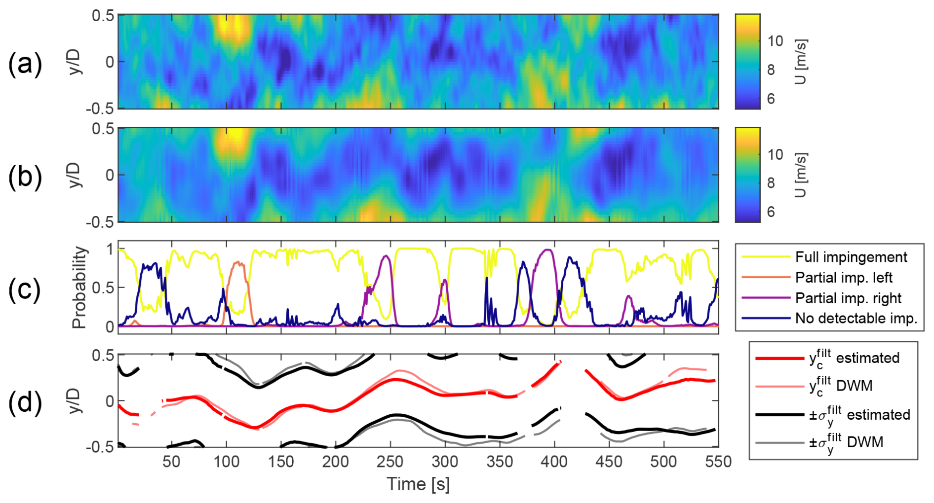
Figure 14 U_amb=10 m s⁻¹, I_amb=9 %, fully impinged. (a) Horizontal slice of the simulated wind field at hub height. (b) Horizontal slice of the estimated wind field at hub height, obtained with the wind sensing model. (c) Classification scores obtained with the wake detection model. (d) Fitted wake properties obtained with the wake characterisation model next to the reference fitted on the raw DWM wind.

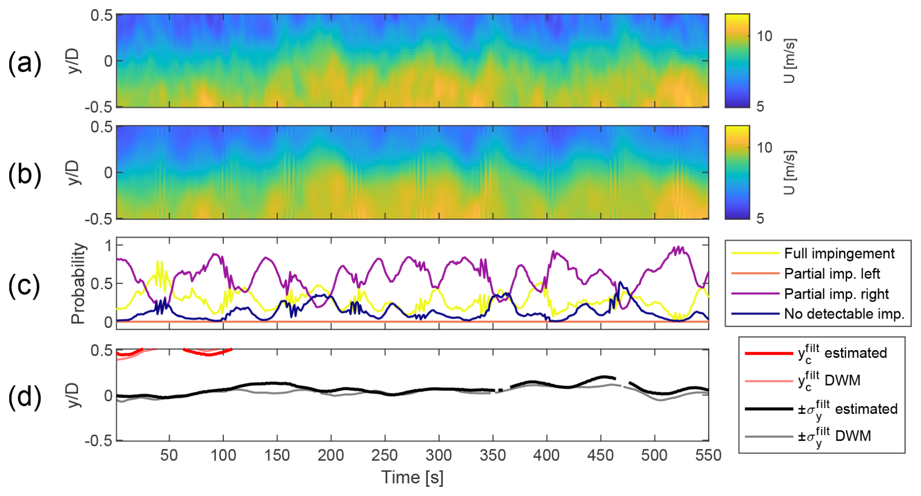
Figure 15 U_amb=10 m s⁻¹, I_amb=3 %, partially impinged. (a) Horizontal slice of the simulated wind field at hub height. (b) Horizontal slice of the estimated wind field at hub height, obtained with the wind sensing model. (c) Classification scores obtained with the wake detection model. (d) Fitted wake properties obtained with the wake characterisation model next to the reference fitted on the raw DWM wind.

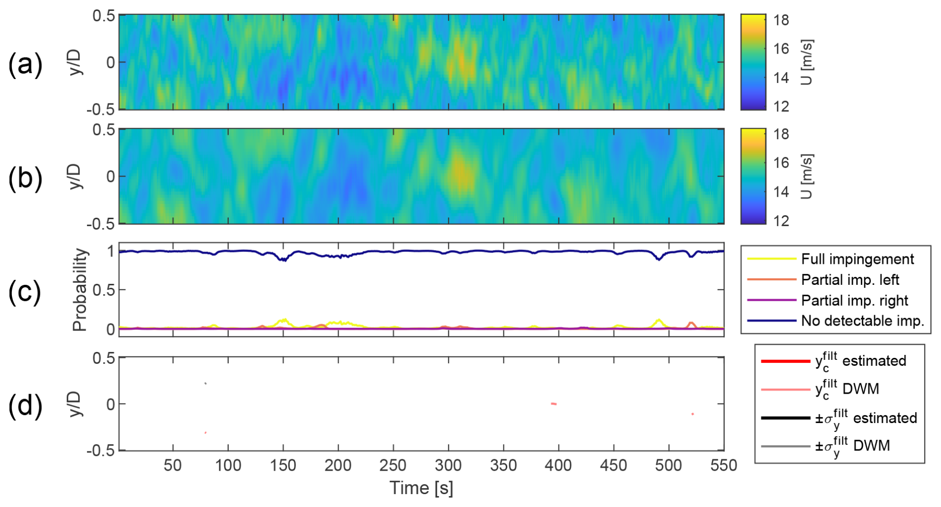
Figure 16 U_amb=15 m s⁻¹, I_amb=5 %, no impingement. (a) Horizontal slice of the simulated wind field at hub height. (b) Horizontal slice of the estimated wind field at hub height, obtained with the wind sensing model. (c) Classification scores obtained with the wake detection model. (d) Fitted wake properties obtained with the wake characterisation model next to the reference fitted on the raw DWM wind.

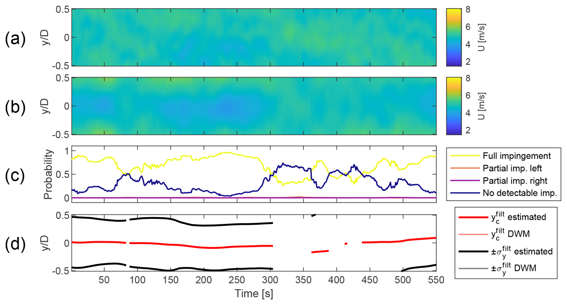
Figure 17 U_amb=5 m s⁻¹, I_amb=5 %, no impingement. (a) Horizontal slice of the simulated wind field at hub height. (b) Horizontal slice of the estimated wind field at hub height, obtained with the wind sensing model. (c) Classification scores obtained with the wake detection model. (d) Fitted wake properties obtained with the wake characterisation model next to the reference fitted on the raw DWM wind.

Figures 14 and 15 compare the performance under high and low I_amb, respectively. They also exhibit different degrees of wake–rotor overlap, allowing us to investigate both full- and partial-impingement scenarios. Figures 16 and 17 show the performance in a scenario with no turbines upstream of the “receiver” device. They show the effects of operating under low- and high-U_amb conditions, respectively.

Quantitative metrics for wake characterisation accuracy are computed as shown in Eqs. (12) and (13). Using the reference derived from raw DWM wind fields (see Sect. 3.1), RMSE is calculated over the time series of both the lateral wake centre and the wake width. Samples classified as “no detectable impingement”, containing NaN values as discussed in Sect. 2.5, are excluded from the calculation.

$$\begin{array}{}\text{(12)}& {\displaystyle }& {\displaystyle }{\mathrm{RMSE}}_{\mathrm{char}}^{y_{\mathrm{c}}}=\sqrt{{\displaystyle \frac{\mathrm{1}}{n_t}}\sum _{i=\mathrm{0}}^{n_t}{\left(y_{\mathrm{c},i}^{\mathrm{filt}}\left(\mathrm{est}\right)-y_{\mathrm{c},i}^{\mathrm{filt}}\left(\mathrm{DWM}\right)\right)}^{\mathrm{2}}}\text{(13)}& {\displaystyle }& {\displaystyle }{\mathrm{RMSE}}_{\mathrm{char}}^{{\mathit{\sigma }}_y}=\sqrt{{\displaystyle \frac{\mathrm{1}}{n_t}}\sum _{i=\mathrm{0}}^{n_t}{\left({\mathit{\sigma }}_{y,i}^{\mathrm{filt}}\left(\mathrm{est}\right)-{\mathit{\sigma }}_{y,i}^{\mathrm{filt}}\left(\mathrm{DWM}\right)\right)}^{\mathrm{2}}}\end{array}$$

Here n_t is the simulation duration; $y_{\mathrm{c},i}^{\mathrm{filt}}\left(\mathrm{est}\right)$ and ${\mathit{\sigma }}_{y,i}^{\mathrm{filt}}\left(\mathrm{est}\right)$ are the estimated $y_{\mathrm{c}}^{\mathrm{filt}}$ and ${\mathit{\sigma }}_y^{\mathrm{filt}}$ at time i, respectively; and $y_{\mathrm{c},i}^{\mathrm{filt}}\left(\mathrm{DWM}\right)$ and ${\mathit{\sigma }}_{y,i}^{\mathrm{filt}}\left(\mathrm{DWM}\right)$ are $y_{\mathrm{c}}^{\mathrm{filt}}$ and ${\mathit{\sigma }}_y^{\mathrm{filt}}$ at time i from the reference fitted on the raw DWM wind, respectively.

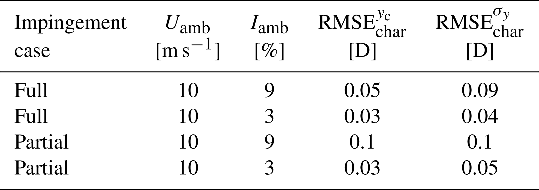
Table 6 shows the wake characterisation RMSE calculated for four example wind fields, comparing the model's accuracy for full and partial wake impingement under high and low I_amb. For brevity, only two of these wind fields are visualised in Figs. 14 and 15. Wind fields in which the DWM reference primarily shows “no detectable impingement” – such as those in Figs. 17 and 16 – are excluded from the RMSE analysis, as the reference wake characterisation mostly contains NaN values.

Table 6 Performance metrics for wake characterisation.

4 Discussion

4.1 Evaluation methods

The reference for wake detection is based on the classifications from a detector trained with simulated (rather than estimated) wind fields. This allows us to consider the effects of varied wake dispersion under different ambient conditions and arguably fits this analysis better than a general impingement definition based strictly on inflow angle. Indeed, to the best of the authors' knowledge, there is not a widely recognised definition of wake impingement (e.g. by means of reduced power output) that could be used here instead.

Wake characterisation accuracy is evaluated by processing the raw DWM wind with the methods from Sect. 2.5, thus extracting reference wake properties. This approach is preferred over taking the “ground truth” from the meandering wake centres applied internally in the DWM model, as turbulent fluctuations in the synthetic wind field – along with additional imposed turbulence – can cause the actual wake experienced by the turbine to deviate from the calculated position. Moreover, this method naturally accommodates the interaction of multiple, combined wakes. A reference derived by fitting a Gaussian profile on a simulated wind field has been used in other studies (Lejeune et al., 2022).

However, it should be noted that using the same methodology to both perform estimations and establish a reference, with the only major difference being the source of the wind field, carries a bias. This is especially relevant for calculated wake characterisation metrics; calculated RMSE values could be expected to increase with the use of a different reference approach. In future work, we aim to address this through validation with higher-fidelity simulations and wind field data.

4.2 Framework performance

4.2.1 Wind sensing

Although there are minor discrepancies for specific wind conditions, the developed wind sensing model presents generally good performance with low error between reference and estimated values. Figure 11 reveals that the wind field reconstruction quality is the highest at the radial distance of approximately half of the rotor radius. This is likely due to the fact that the flow impacting the mid-blade region has the largest influence on the root bending moments. The YZ locations outside of the rotor plane yield the highest RMSE due to blade sensors being unable to meaningfully react to the flow fluctuations from that region. Figures 14 and 15 show that major flow fluctuations are well captured in the estimated wind field representations. Some smoothing occurs for smaller-scale fluctuations, but this does not pose a major problem for wake detection. In fact, the attenuation of less significant turbulent eddies allows the wind sensing procedure to act as a spatial filter, focusing on larger flow structures like a wake deficit. The sensitivity study from Sect. 3.3 shows that the normalised $\stackrel{\mathrm{‾}}{{\mathrm{RMSE}}_{\mathrm{sen}}}$ rises with increasing I_amb, which can be attributed to the higher flow complexity in more turbulent wind. The cause of higher error in low-U_amb cases is investigated in Fig. 17. The wind field reconstruction shows a minor U deficit that is not present in the simulated wind field, which is identified by the CNN as a wake impingement. This phenomenon occurs for the majority of wind directions at U_amb=5 m s⁻¹ (see Fig. 12a), which in turn is the cause of high wake detection RMSE captured in Table 5. Looking at the high-U_amb case in Fig. 16, it is apparent that a more heterogeneous wind field effectively disperses such anomalies. This emergence of “fake” wakes under low-wind-speed conditions is likely a result of the training dataset composition, 75 % of which shows wake impingement, leaving only 25 % for purely ambient turbulence cases. Using a single wind sensing estimator across these cases introduces a bias, as the model is predominantly trained on wake impingement conditions. The misclassification between “fully impinged” and “no detectable impingement” is quantified by the confusion matrix in Fig. 9.

4.2.2 Wake detection

Examining both Fig. 12 and Fig. 13, most plots show the wakes generated by upstream turbines to be correctly identified for the corresponding wind directions at the “receiver” turbine. There is a distinct difference in the proportion of samples identified as a wake depending on the distance between the “emitter” and “receiver”. For turbines further away, the proportion of detected impingement is lower due to the wake losing its distinctive shape over a longer distance and interacting with the turbulent atmospheric boundary layer for a longer time. This relationship is evident in both the number of “impingement” samples per simulation (length of the blue/orange peak) and the number of wind directions for which the wake is detected (width of the blue/orange peak).

The superposition of wakes does not appear to have a significant effect on wake detection performance. Wakes from eastern turbines (a single machine upstream) do not yield substantially different wake detection results than wakes from deep inside the wind farm to the west. This is likely a consequence of the wake superposition approach used, where wind speed at each YZ grid point on the receiving turbine is derived based on the strongest influencing wake deficit. As a result, the primary aspect impacting the wake detection performance is the distance between the “receiver” and “emitter” machines. This is also due to limiting the training data to one pair of “emitter”–“receiver” turbines at a fixed distance.

As shown in Table 5, the wake detection RMSE largely follows the trends from the wind sensing RMSE. This is expected, as one model uses the outputs from the other. The highest error across all cases is reported for ambient wind speed of 5 m s⁻¹, which is due to the wind sensing anomaly described above. The wake detection is progressively more accurate with increasing U_amb (attributed to dispersion of the anomaly), until the RMSE begins to rise above 11 m s⁻¹. Visual inspection of Fig. 12e and f reveals that this is a consequence of increased estimation–reference mismatch at the wind directions with high impingement ratios. These wind speeds usually correspond to above-rated operation, where the wakes are less pronounced due to decreased thrust, likely making them more difficult to detect. The wake detection RMSE rises with increasing I_amb values; the plots in Fig. 13 show that the main source of the error is increasing “noise” of some wake impingement detected for all of the wind directions. This is expected, as more turbulent wind fields contain more large-scale ambient eddies that could be identified as a wake.

The sample-by-sample classification is presented in the (c) plots in Figs. 14 to 17. The CNN's output aligns with the respective wind slice samples; for example, when wake meanders from the centre to the Y-positive part of the snapshot, the highest probability transitions from “full impingement” to “partial impingement left”. This indicates that the instantaneous wake position can be, at least to some extent, tracked even without a dedicated wake characterisation model.

4.2.3 Wake characterisation

Figures 14 and 15 show the sample-by-sample wake deficit characterisation for two example wind fields. Visual comparison between the simulated wind field in the (a) plots and characterised wake in the (d) plots shows that the wake behaviour is appropriately captured in both cases. The estimated wake properties fit the reference values reasonably well. The time series of the fitted wake centre and lateral border are near continuous for lower I_amb, while higher I_amb yields a characterisation with a few gaps. This is due to the removal of samples classified as the “no detectable impingement” class, which happens more often when the deficit shape is distorted by increased ambient turbulence. Table 6 brings further insight, showing quantitative characterisation accuracy metrics for full and partial impingement under low and high I_amb. As expected, higher turbulence causes the estimated wake properties to diverge more from the reference, thus increasing the RMSE. For all wind fields, the error is higher for σ_y than for y_c, likely due to the wake centre being more easily identified by the least squares algorithm (it is simply the area with the lowest value). Error comparisons between full and partial impingement reveal mostly similar values, with the only outlier being RMSE${}_{\mathrm{char}}^{y_{\mathrm{c}}}$ at I_amb=9 %, where the partial wake error is twice that of the full wake. This is a logical outcome, given the increased difficulty of characterisation when the wake meandering motion is strong and the centre is outside the YZ snapshot.

Figure 17d shows how the “fake” wake anomaly discussed above results in a characterisation performed on ambient turbulence. This effect is gone when U_amb is higher (see Fig. 16d), which is why the characterisation is missing for the entire wind field except a few isolated samples.

4.3 Applicability

Overall, the presented performance shows that the developed methodology is a promising solution to the challenging problem of generalised wake impingement estimation. The less accurate wake detection for U_amb values of 5 and 15 m s⁻¹ is less critical after the consideration of specific application of this work. Firstly, at U_amb=5 m s⁻¹ the turbine is usually close to its cut-in wind speed (Carrillo et al., 2013), meaning that for many cases, applying flow control would not be necessary. Secondly, the wind farm flow control brings the largest benefits for below-rated operation, where, due to higher energy extraction and lower wind, the wakes are more pronounced (Scott et al., 2024). These conditions align with the scenarios where the framework demonstrates optimal performance. Wind speeds above 13 m s⁻¹ (where the framework performance deteriorates) are generally less frequent than lower-wind-speed conditions (Shu and Jesson, 2021), further mitigating the impact of these issues. A similar comment can be made with respect to wake detection RMSE increasing with I_amb. Wake steering control brings the largest benefits when the wind is less turbulent, which is where the framework shows the best performance.

The presented results also highlight that wake detection accuracy is highly dependent on the training data selection. This indicates that improved performance across a broader range of conditions could be achieved by extension of the training dataset, e.g. by learning the wake deficit shape from various “receiver” turbines. One of the testing subsets has I_amb equal to 9 %, a value outside the training range of 3 %–7 %. While having one of the highest errors in the study, the wakes within this subset are nonetheless detected at correct wind directions. This highlights the framework's ability to produce reasonable results for wind fields with ambient conditions “unknown” to the estimator. This is highly advantageous for the field application context, where the pre-deployment training procedure would only capture some of the wind effects experienced by the wind farm.

4.4 Current limitations

The present methodology treats each YZ wind snapshot entirely independently. It therefore seems clear that improved performance (and solutions for some of the problematic cases which are identified) could be readily achieved by extending the methodology to undertake a post-processing analysis which accounts for time variations in results. This could, for example, allow for the imputation of gaps that occur in characterised time series for more turbulent wakes (see Fig. 14); moreover, by considering classifications of time-adjacent snapshots, it could help in the correct detection of fully impinged cases which are misidentified as unimpinged. Kalman filtering appears to be a technique well suited to these possible methodological extensions.

It should also be highlighted that the application of a moving average filtering within the methodology results in predictions lagging behind the true wind field. This lag ranges from approximately 12 s for U_amb=15 m s⁻¹ to approximately 58 s for U_amb=5 m s⁻¹. These values are a consequence of matching the filtering window width to the wind field's typical meandering timescales (see Eqs. 7 and 8). In the context of wind farm flow control, these levels of lag are not necessarily problematic, and the lag may be removable by introducing methods such as Kalman filtering. Relevant literature (Luo et al., 2024; Zhou et al., 2023) shows that long short-term memory networks could potentially provide a short-term forecast of the wake dynamics, thus providing an alternative solution. Further research needs to be conducted to investigate these leads.

Note also that the range of ambient turbulence intensities used for framework testing falls between 3 % and 9 %, and the atmospheric conditions for both training and testing are considered neutral. Large offshore wind farms could experience higher levels of turbulence deep within the turbine grid due to multiple wake interactions (Shaw et al., 2022). These simplifications should be acknowledged, and other turbulence levels, along with incorporating both stable and unstable boundary layer conditions, should be analysed in future work. Similarly, turbine yaw offsets are also not considered in this work. The current analysis implemented a medium-fidelity wake model, and so further work should also extend this framework to more realistic wake structures, for example, those obtained through large-eddy simulations.

5 Conclusions

The proposed method for generalised wake impingement detection and characterisation shows good performance for a wide range of tested wind conditions. The framework's effectiveness is sensitive to ambient wind speed and turbulence intensity levels, with the best performance observed for wind speeds between 7 and 13 m s⁻¹ and turbulence intensities ranging from 3 % to 7 %. Wind field reconstruction reports high accuracy with an all-around RMSE of 3.7 % when normalised by mean ambient wind speed. The wake detection model correctly responds to the wake presence; averaging the RMSE across all wind fields used in testing indicates that the correct wake impingement case is identified for approximately 77 % of the samples. Wake characterisation appropriately adapts to the meandering motion, achieving high accuracy; wake centre tracking reports an average RMSE of 0.08 and 0.03 D for I_amb of 9 % and 3 %, respectively; and wake lateral border tracking reports an average RMSE of 0.1 and 0.05 D for I_amb of 9 % and 3 %, respectively. This work provides a baseline concept for generalised wake impingement estimation, which, with further improvements, could greatly contribute to better-informed wind farm flow control. Current limitations are identified, with the most important including the shortcomings of the evaluation methods and anomalies in wind sensing. Next steps for the further development of this framework include validation of the current setup in progressively more realistic environments (including yaw misalignment, higher-fidelity wind fields and wakes, and utilisation of field data), an extension of the training dataset (towards accounting for more flow phenomena from more turbines at different distances), and methodological extension to capture time variance between individual two-dimensional snapshots and opportunities for imputation and forecasting of wake properties. Kalman filtering is identified as a likely route to extending the framework in this manner.

Appendix A: Convolutional neural network

CNNs are a specialised type of deep learning method, optimised for working with grid-like data (most commonly two-dimensional images). Their design is perfectly suited for learning spatial features from input data, making them especially effective for image recognition and classification tasks. Due to several key achievements in recent years, they have revolutionised areas such as facial recognition, handwriting analysis and autonomous vehicles (Li et al., 2022). In the context of wind energy, some examples of CNN implementation include wind power prediction (Zhu et al., 2017; Harbola and Coors, 2019) and early fault detection and classification (Rahimilarki et al., 2022). The input layer of the CNN is the size of the grid-like data it processes – in a simple example of a grey-scale image, it would be its width multiplied by its height. If the task at hand is to classify the image, for example, determining which handwritten digit the image shows, then the output layer would consist of 10 nodes (one for each digit), each holding a confidence value between 0 and 1. The actual processing occurs in the hidden layers located between the input and output layers, and for most CNNs, these layers are a combination of the following:

• Convolutional layer. This layer applies learnable filters (also called kernels) that slide across the input data, only working on a small patch of the data at a time. A dot product of the kernel and data at each position creates a measure of how close a patch of data resembles a given spatial feature, such as an edge or arch. Doing this for the entire input results in a feature map. Performing this operation through multiple iterations with many kernels, progressively optimising their weights, allows us to combine small features into larger ones and is ultimately the key to detecting patterns.

• Activation function. Normally following the convolution layers, various activation functions like the rectified linear unit (ReLU) introduce non-linearity, enabling the network to learn complex patterns. It is achieved by restricting the connections between the neurons when the weighted sum is too low.

• Pooling layers. The pooling layers reduce the spatial size of feature maps, decreasing computational complexity and helping to prevent overfitting. Max pooling is the most commonly used method of doing so, selecting the maximum value from each patch of the feature map.

• Fully connected layer. After several cycles of convolution–activation–pooling, this layer connects every neuron in one layer to every neuron in the next, combining features learned by previous layers to produce final predictions.

While designing the neural network, one needs to decide on the number and type of hidden layers implemented in its architecture, as well as on the hyperparameters such as the number and size of learnable filters. Moreover, as with all deep learning techniques, the performance of the CNN is heavily dependent on the quality of data used for its training.