Spectral proper orthogonal decomposition of active wake mixing dynamics in a stable atmospheric boundary layer

Recent advancements in the use of active wake mixing (AWM) to reduce wake effects on downstream turbines open new avenues for increasing power generation in wind farms. However, a better understanding of the fluid dynamics underlying AWM is still needed to make wake mixing a reliable strategy for wind farm flow control. In this work, a spectral proper orthogonal decomposition (SPOD) is used to analyze the dynamics of coherent flow structures that are induced in the wake through blade pitch actuation. The data are generated using the ExaWind software suite to perform large eddy simulations of an NREL 2.8 MW turbine operating in a stable atmospheric boundary layer. SPOD tracks the modal behavior of flow structures from their generation in the turbine induction field through their growth in the near-wake region and to their subsequent evolution and energy transfers in the far wake. SPOD is shown to be a useful tool in the context of AWM because it translates the wavenumber and frequency inputs to the turbine controller to structures in the wake. A decomposition of the radial shear stress flux in the wake is also developed using SPOD to measure the contribution of coherent flow structures to mean flow turbulent entrainment and wake recovery. The effectiveness of AWM is connected to its ability to excite inherent structures in the wake of the turbine that arise using baseline controls. The effects of AWM on blade loading are also analyzed by connecting the axial force along the blade to the SPOD analysis of the turbine induction field. Lastly, the performance of different AWM strategies is demonstrated in a two-turbine array.

1 Introduction

Interactions between wind turbines and surrounding wakes often result in reduced power generation and increased structural loads for downstream turbines in a wind farm (Nygaard, 2014; El-Asha et al., 2017). Power losses are particularly problematic in stable atmospheric boundary layers (ABLs) because of the increased persistence of wind turbine wakes in these conditions. Several wind farm flow control (WFFC) methods have been proposed in the last decade to reduce the negative impacts of wake momentum loss in wind farms, including turbine derating, wake steering, and wake mixing (Meyers et al., 2022). These methods rely on static or dynamic adjustments to the operation of upstream turbines, away from their optimal set-point, for the benefit of downstream turbines. This paper focuses on the technique of active wake mixing (AWM), which is a particularly promising approach for wake mitigation as it provides a mechanism for introducing new momentum into a wind farm. Specifically, AWM aims to excite coherent structures in the wake through dynamic oscillations in the turbine's control parameters to enhance the entrainment of higher velocity flow into the wake, resulting in faster wake recovery.

As with any WFFC strategy, AWM introduces power and load trade-offs to the wind farm optimization problem. Recent experimental and numerical results indicate that AWM can improve the power production of turbine arrays anywhere from 1 % to 30 % (Frederik et al., 2020a, b, c; Yılmaz and Meyers, 2018; Taschner et al., 2023), at the cost of increasing loads on upstream turbines due to pitch actuation (Frederik and van Wingerden, 2022). These results vary significantly with wind farm layout, turbine model, and ABL condition. Additionally, the design space for AWM is considerably large. While wake steering, for example, depends on setting the yaw angle, common implementations of AWM involve several relevant design parameters to control the blade pitch fluctuations, such as the pitch amplitude, forcing frequency and wavenumber, clocking angle, and waveform of the pitch signal (see Cheung et al., 2024, and Sect. 2). Given the complex interactions between wind conditions, wind farm layout, and turbine control parameters, we therefore cannot expect to rely solely on parametric studies to optimize AWM. Instead, a deeper understanding of the physical mechanisms behind the power and load trade-offs of AWM is necessary to effectively navigate the design space.

AWM introduces periodic oscillations in the turbine's control parameters, such as the blade pitch, to generate large-scale coherent structures in the wake. Several approaches have been developed in the recent literature to analyze the dynamics induced by these large-scale structures and their connection to the performance of different AWM strategies. Brown et al. (2025) analyzed the mean flow kinetic energy budget through a control volume analysis around the wake of an actuated turbine. This analysis was used to explain the power increases for a two-turbine array reported by Frederik et al. (2025). It was shown that AWM enhances the turbulent and, in some cases, the mean flow entrainment of momentum into the wake and that veer has a large impact on the relative performance among AWM strategies. Korb et al. (2023) noted the importance of turbulent entrainment as well but also showed that helical structures in particular can spread and deflect the wake deficit, leading to faster wake recovery. Munters and Meyers (2018) used an adjoint framework to determine an optimal perturbation to impart on the wake, which resembled an axisymmetric flow structure that enhanced existing vortical structures in the non-actuated wake. Cheung et al. (2024) introduced a normal-mode representation of the coherent wake structures and used a linear stability analysis to quantify the growth characteristics of the initial flow disturbances in the wake.

Despite these advancements, a complete understanding of the performance differences between AWM strategies has not been established, including their impact on wake dynamics and relationship with ABL characteristics, which limits the applicability of wake mixing technologies in practice. Fortunately, large-scale coherent structures are a well-studied phenomenon in the broader context of turbulent flows (Hussain and Reynolds, 1970; Robinson, 1991; Ho and Huerre, 1984; Crow and Champagne, 1971; Fuchs et al., 1979), and several techniques have been developed to extract, quantify, and model coherent flow features (Rowley and Dawson, 2017; Taira et al., 2017). The spectral proper orthogonal decomposition (SPOD), in particular, has proven to be a useful representation of space–time coherence in statistically stationary flows (Towne et al., 2018). Since its introduction by Lumley (1967), SPOD has been applied to a number of turbulent flows, including turbulent boundary layers (Tutkun and George, 2017), jets (Citriniti and George, 2000; Gudmundsson and Colonius, 2011), and wakes (Tutkun et al., 2008; Araya et al., 2017). In the context of AWM, Cheung et al. (2024) demonstrated in a canonical flow that SPOD could be used to track the modal growth of instabilities in the wake. Other related data-driven methods also exist, such as space-only proper orthogonal decomposition (POD) and dynamic mode decomposition (DMD), which provide spatial and temporal orthogonalizations of the flow, respectively. DMD has recently been used to analyze flow structures (Muscari et al., 2022) and model wake dynamics (Gutknecht et al., 2023) in the context of AWM. While these methods are effective at identifying either spatially coherent structures or dynamically meaningful temporal structures in the flow, SPOD identifies structures that evolve coherently in both space and time. Furthermore, as demonstrated by Towne et al. (2018), the SPOD structures correspond to an ensemble average of DMD structures, so that the SPOD structures are both dynamically significant, unlike those identified by space-only POD, and provide an optimal description of the energy content in the flow.

In this paper, the applicability of SPOD to AWM is further strengthened. A formulation of SPOD is presented that translates the wavenumber and frequency inputs to the turbine controller to coherent structures in the flow. The coherent structures induced by AWM are then analyzed from the turbine induction field to the far-wake region using high-fidelity large eddy simulation (LES) data of a wind turbine operating in stable ABL conditions. SPOD is used to quantify the energetic structures in the wake for each AWM strategy, as well as their interactions with other large-scale wake structures. Additionally, the SPOD analysis is connected to conventional wake mixing metrics through a modal decomposition of turbulent entrainment statistics. This formulation provides insights into the wake recovery mechanisms of different AWM strategies and their relative performance, which is subsequently demonstrated in a two-turbine array. The flow structures that arise in the wake of a baseline-operated turbine are also analyzed through SPOD and connected to the performance of different AWM strategies.

The remainder of this paper is organized as follows: the methodology for the paper is discussed in Sect. 2, including the LES specifications, ABL precursor generation, turbine model, implementation of AWM in the turbine controller, and SPOD formulation. The results from the SPOD analysis are then discussed in Sect. 3.1 for several AWM strategies, which are connected to conventional wake mixing metrics in Sect. 3.2 and turbine performance metrics in Sect. 3.3. Finally, conclusions are provided in Sect. 4.

2 Methodology

2.1 LES formulation

LESs of a single wind turbine are performed using the ExaWind Nalu-Wind solver. Nalu-Wind employs an unstructured second-order control volume finite-element discretization in space and a second-order backwards differentiation scheme in time to solve the implicitly filtered incompressible Navier–Stokes equations. Additional details on the Nalu-Wind solver and its application to wind turbine simulations is given by Sprague et al. (2020) and Domino (2015). A one-equation model for the evolution of the subgrid turbulent kinetic energy (TKE) is used to represent the subgrid-scale effects on the resolved flow (Davidson, 1997). The simulation domain ranges from $\mathrm{0}\mathrm{m}\le x\le \mathrm{3000}\mathrm{m}$, $\mathrm{0}\mathrm{m}\le y\le \mathrm{750}\mathrm{m}$, and $\mathrm{0}\mathrm{m}\le z\le \mathrm{960}\mathrm{m}$ in the streamwise, lateral, and vertical directions, respectively. A 3-D visualization of the flow on a subset of the domain is shown in Fig. 1. Three distinct levels of isotropic resolution are used to discretize the domain around the turbine: a 5 m background mesh near the domain boundaries; a 2.5 m refinement zone that extends 10 D in the streamwise direction and 1.8 D in the lateral and vertical directions from the domain center; and a 1.25 m refinement box surrounding the turbine, extending 2 D upstream and downstream of the turbine, and 1 D in the vertical and lateral directions from the turbine's hub location.

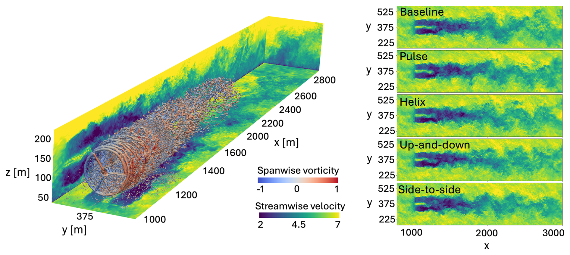
Figure 1 (Left) 3-D visualization of the flow for the pulse case with A=1.25° pitching amplitude. Isosurfaces of the Q criterion (Q=0.05) are shown on a subset of the domain, colored by spanwise vorticity. Mid-planes of the wake are projected to the domain boundaries and show streamwise velocity. (Right) contours of streamwise velocity for each AWM strategy on the hub height plane.

The streamwise and lateral boundary conditions are defined by an inflow condition extracted from an initial precursor simulation. The target conditions for the precursor simulation are derived from stable ABL measurements taken in 2021 and concurrent with the American Wake Experiment (AWAKEN) campaign (Moriarty et al., 2024). Specifically, the atmosphere was sampled at the Department of Energy's Atmospheric Radiation Measurement (ARM) Southern Great Plains (SGP) C1 site (Facility, 2024) using a Doppler profiling lidar and CO₂ flux stations. A number of filters were applied to isolate 30 min bins corresponding to high-quality measurements and periods of likely interest for wake control. Balancing the need for an appreciable sample size with that for retaining the realism of a specific observable ABL condition, the latter filters isolated a wind condition with a frequency of occurrence: wind speed of 6–6.7 m s⁻¹, wind direction ranging from 100 to 260° (assuming a clockwise definition of wind direction with 0° corresponding to a northerly flow), and turbulence intensity (TI) from 0 % to 7 %. The 1200 min of (non-contiguous) data that meet the above criteria are used to establish target statistics for the precursor simulation, and these have a hub height wind speed of 6.4 m s⁻¹, a TI of 4.4 %, a shear exponent of 0.19, and 17° of veer over the rotor disk. The low TI and high veer in this target are congruent with the southerly stable ABL conditions typically observed at the SGP site (Krishnamurthy et al., 2021), and these conditions offer a strong opportunity to demonstrate a use case for wake control technology.

The surface roughness height (0.0015 m) and cooling rate ($\mathrm{4.16}\times {\mathrm{10}}^{-\mathrm{5}}$ K s⁻¹) parameters are calibrated in the precursor simulation of the ABL to ensure good agreement between the simulated and measured flow statistics; this calibration results in inflow data with an average hub height wind speed of U_∞=6.4 m s⁻¹, a TI of 3.5 %, a shear exponent of 0.17, and 9° of veer over the rotor disk. Notably, the simulated ABL exhibits less veer than the measurement data, and this is due to the numerical forcing scheme used to drive the ABL towards the target statistics (primarily TI and shear), which limits the amount of simulated veer that can be achieved while maintaining a realistic ABL velocity profile; such difficulty achieving high veer was also encountered in Brown et al. (2025) and Frederik et al. (2025). Alternate ABL forcing schemes, such as those which incorporate meso-scale information in a direct assimilation approach, may be able to match the veer and wind speed profiles but are not studied here. In addition to the above summary statistics, a good agreement between the vertical profiles of the simulated and measured ABL is found (see Fig. 2).

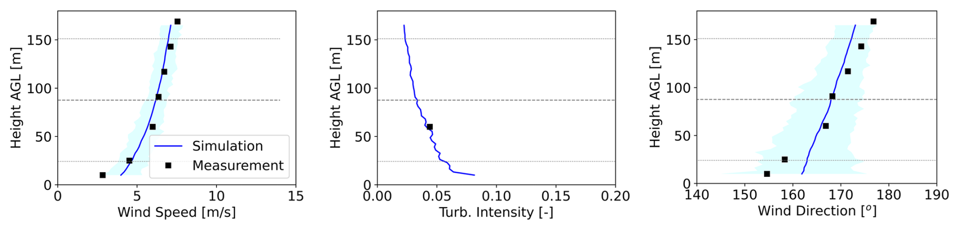
Figure 2 Horizontally averaged profiles of the simulated and measured wind speed, turbulence intensity, and wind direction.

The turbine is simulated in the ABL with a time step of Δt=0.02 for 1100 s after reaching a steady state. Terrain effects are not included in either the precursor or the wind turbine simulations, and, instead, a flat lower surface is implemented using the atmospheric rough wall model from Moeng (1984). A 100 m wide inversion layer is applied to the temperature profile at z=700 m to reduce perturbations in the flow above this height, and a temperature gradient of $\mathrm{7.5}\times {\mathrm{10}}^{-\mathrm{4}}$ K m⁻¹ is maintained at the upper boundary. A potential flow solution is used, setting the upper boundary condition for the velocity field.

The turbine specifications are provided by the NREL 2.8 MW turbine model (Quon, 2024), which provides an open-source representation of a turbine that is similar to those located at the AWAKEN site. The hub of the turbine is located in the computational domain at $(x_{\text{hub}},y_{\text{hub}},z_{\text{hub}})=(\mathrm{1050},\mathrm{375},\mathrm{88.5})$ m, within the Δx=1.25 m resolution region. The wind speed in the precursor ABL simulation at the hub height location corresponds to region 2 for this turbine and also falls within the relatively constant thrust coefficient region (see Fig. 3). To represent the dynamic response of the turbine, Nalu-Wind is coupled to the National Renewable Energy Lab's OpenFAST software suite (National Renewable Energy Laboratory, 2024b), which has been validated vs. measurements of the GE 2.8 MW turbine on which the NREL 2.8 MW turbine is based (Brown et al., 2024). An actuator line model (ALM) with an isotropic Gaussian spreading function with a spreading parameter of $\mathit{\epsilon }/\mathrm{\Delta }x=\mathrm{2}$ is used to represent the turbine aerodynamic forces computed in OpenFAST as body forces in the LES (Sorensen and Shen, 2002). The filtered lifting line correction is applied with an optimal kernel width of ε^opt=0.25c, where c is the chord length, to improve the ALM's representation of the force distribution along the blade (Martínez-Tossas and Meneveau, 2019; Martínez-Tossas et al., 2024).

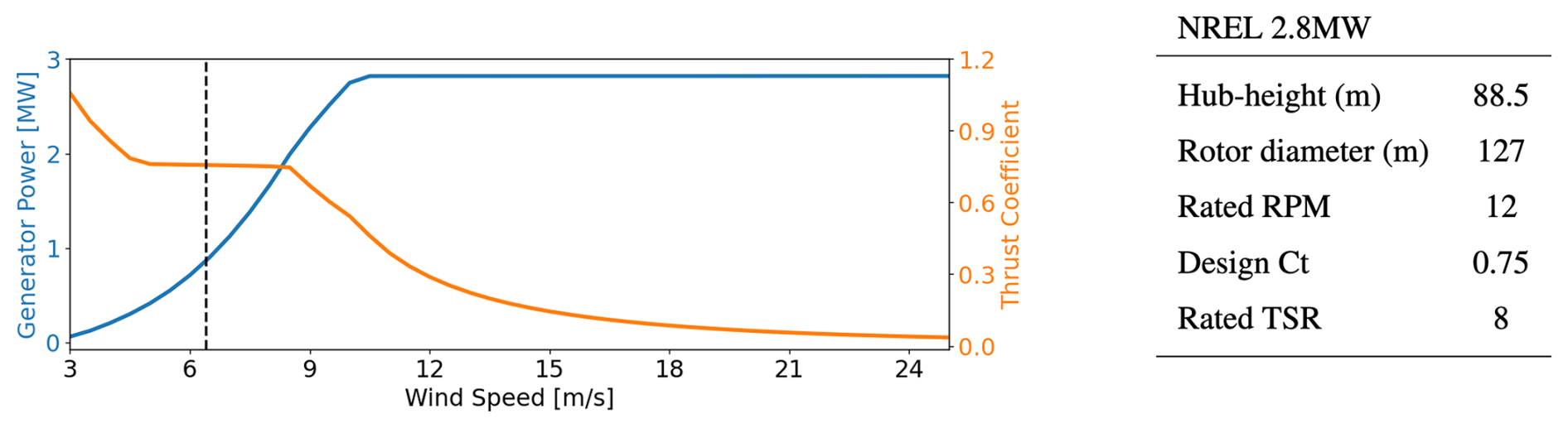
Figure 3 Specifications of the NREL 2.8 MW reference turbine model (Quon, 2024), including the generator power and rotor thrust curves (left) and the design parameters (right). The dashed line corresponds to the hub height wind speed for the precursor ABL simulation used in this study, which is situated in region 2 for this turbine.

To implement different AWM control strategies on the turbine, a dynamic blade pitch Θ is specified on top of the baseline pitch set-point Θ₀. The dynamic blade pitch can be specified using either a normal-mode representation (Cheung et al., 2024) or a Coleman transform representation (Frederik et al., 2020b). Both representations have been implemented in NREL's reference open-source controller (ROSCO v2.8.0; National Renewable Energy Laboratory, 2024a), which is coupled to OpenFAST in the LES. In this work, the normal-mode representation is used because the wavenumber and frequency input to the controller align directly with the parameters of the SPOD analysis formulated in Sect. 2.2. Specifically, the dynamic blade pitch for each blade is specified as

$$\begin{array}{}\text{(1)}& \mathrm{\Theta }\left(t\right)={\mathrm{\Theta }}_{\mathrm{0}}\left(t\right)+A\sum _{\mathit{\left\{}{\mathit{\kappa }}_{\mathit{\theta }}\mathit{\right\}}}\cos ({\mathit{\omega }}_{\mathrm{e}}t-{\mathit{\kappa }}_{\mathit{\theta }}\mathit{\theta }(t)+{\mathit{\varphi }}_{\text{clock}}),\end{array}$$

where A is the pitching amplitude, ω_e is the excitation frequency, θ is the azimuth position of the blade, ϕ_clock is the clocking angle, and κ_θ is an azimuthal wavenumber. The summation in Eq. (1) is over a discrete set of azimuthal wavenumbers. Of particular importance to this study are the κ_θ and ω_e parameters, which control the shape and frequency of the flow structures that are imparted on the wake, respectively. The excitation frequency can be specified through a Strouhal number based on the inflow velocity U_∞ and turbine diameter D as ${\mathit{\omega }}_{\mathrm{e}}=\mathrm{2}\mathit{\pi }\mathit{\text{St}}{U}_{\mathrm{\infty }}/D$. A Strouhal number of St=0.3 is used for all control strategies considered here, as this has been shown in previous studies to align with natural unsteady processes in the wake and result in good performance for different AWM cases (Frederik et al., 2020c; Munters and Meyers, 2018; Cheung et al., 2024). A single Strouhal period based on the inflow velocity and turbine diameter corresponds to 66.15 s, which means that flow structures are generated over much longer periods than a typical rotor period (see Fig. 4). The 1100 s of simulation time corresponds to over 16 complete Strouhal cycles at St=0.3.

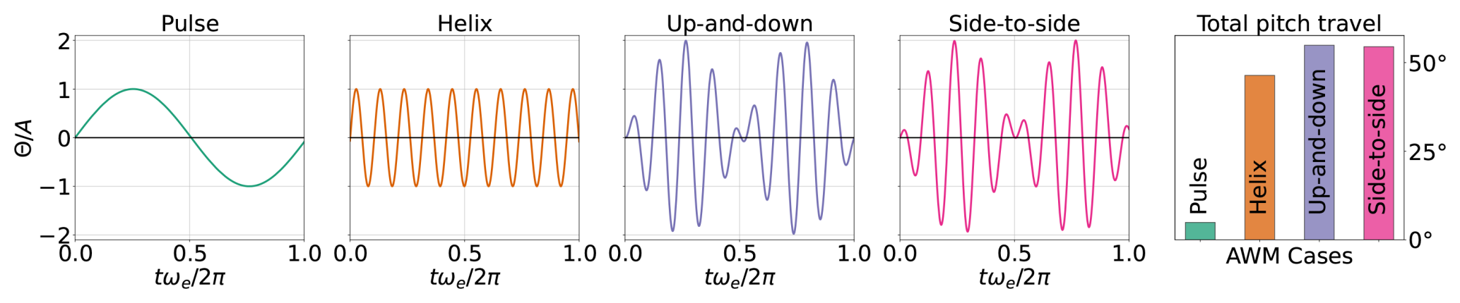
Figure 4 Time series of the blade pitch signal for a single blade for each AWM case, normalized by the pitching amplitude. One Strouhal period is shown based on the excitation frequency ω_e. The black line at $\mathrm{\Theta }/A=\mathrm{0}$ corresponds to the baseline blade pitch signal. The total pitch travel for a single Strouhal period is also shown for each AWM case.

Four AWM strategies are considered in addition to a baseline case, including a pulse (κ_θ=0), helix (${\mathit{\kappa }}_{\mathit{\theta }}=-\mathrm{1}$), side-to-side (${\mathit{\kappa }}_{\mathit{\theta }}=\pm \mathrm{1}$, ϕ_clock=90°), and up-and-down (${\mathit{\kappa }}_{\mathit{\theta }}=\pm \mathrm{1}$, ϕ_clock=0°) actuation. Here, positive and negative azimuthal wavenumbers denote flow structures that rotate in the same and opposite direction of the turbine, respectively (i.e. clockwise and counter-clockwise when looking downstream). The counter-clockwise helix method is used here, which has been found to consistently outperform its clockwise counterpart (Coquelet et al., 2024). The pulse forcing is axisymmetric and achieved through collective pitching of the three turbine blades, while the other AWM strategies rely on individual pitch control to create a non-uniform thrust force around the rotor disk. In this study, the clocking angle is only relevant for differentiating the side-to-side and up-and-down actuations, in which case it negates the thrust force in the vertical and horizontal directions, respectively. For the pulse and helix cases, the clocking angle only determines the phase of excitation, and it is arbitrarily set to 90° here. A pitching amplitude of A=1.25° is primarily used in this study, although other values of A are also discussed.

The blade pitch signal for each AWM case is shown in Fig. 4 over a single Strouhal period. For the up-and-down and side-to-side cases, a pitching amplitude of A=1.25° is applied to both the ±1 modes. This choice is made to ensure that each mode is forced with the same pitch amplitude, allowing for a consistent comparison of modal energy and entrainment between modes and AWM cases in the SPOD analysis developed in Sect. 2.2. As a result, the total pitch amplitude for the up-and-down and side-to-side cases is twice that of the pulse and helix cases; however, this corresponds to only an 18 % increase in total pitch travel over the helix case (see Fig. 4). A summary of the AWM parameters is provided in Table 1, and a visualization of the streamwise velocity on the hub height plane for each AWM strategy is shown in Fig. 1.

Table 1 Summary of AWM cases and control settings.

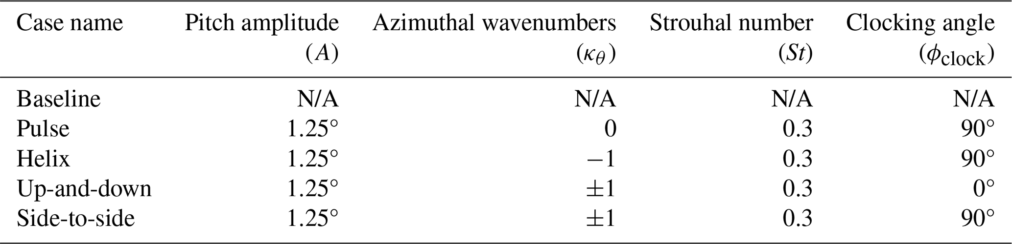
N/A: not applicable.

The blade pitch fluctuations are designed to induce azimuthal and temporal variations in the blade loading at the wavenumbers and frequencies input to the controller. These variations can be examined through the spectrum of the axial force along the blade span (Cheung et al., 2024). The Fourier representation of the axial force F_x at a particular radial location r, blade azimuthal angle θ, and time t for a given blade is

$$\begin{array}{}\text{(2)}& {\displaystyle }{\displaystyle }{\widehat{F}}_x(r,{\mathit{\kappa }}_{\mathit{\theta }},\mathit{\omega })=\int \int F_x(r,\mathit{\theta },t){\mathrm{e}}^{-\mathrm{i}(\mathit{\omega }t+{\mathit{\kappa }}_{\mathit{\theta }}\mathit{\theta })}\mathrm{d}\mathit{\theta }\mathrm{d}t.\end{array}$$

Given a discrete time series of the axial force at each nodal location along the blade F_x(r,t), the blade azimuthal angle is determined using the instantaneous rotor speed signal Ω, as $\mathit{\theta }\left(t\right)=\mathit{\theta }\left(\mathrm{0}\right)+{\int }_{\mathrm{0}}^t\mathrm{\Omega }\left(t^{\prime }\right)\mathrm{d}{t}^{\prime }$. Then the Fourier coefficients ${\widehat{F}}_x$ are readily determined by performing a Fourier transform in the time and azimuthal directions.

The blade loading spectra indicate that the prescribed blade pitch fluctuations result in the intended modal response in the axial loading for each AWM strategy (see Fig. 5). In all cases, the highest periodic loading occurs near the blade tip at around 90 % of the blade span. Notably, the κ_θ=0 actuation exhibits significantly higher periodic loading at St=0.3 than the other cases. An increase in the axial force of over 10 % is observed at the κ_θ=0 wavenumber for the pulse actuation across the majority of the blade span, while the other cases show around a 7.5 % increase in their respective modes. There are contributions to the axial force from wavenumbers other than those directly forced by the prescribed blade pitch fluctuations, which may result from factors such as the unsteady inflow, the effects of AWM on the turbine induction field, or other controller specifications. For instance, the non-axisymmetric forcing strategies exhibit a notable increase in the κ_θ=0 mode, which is attenuated 2.5 % for the up-and-down case in the middle of blade.

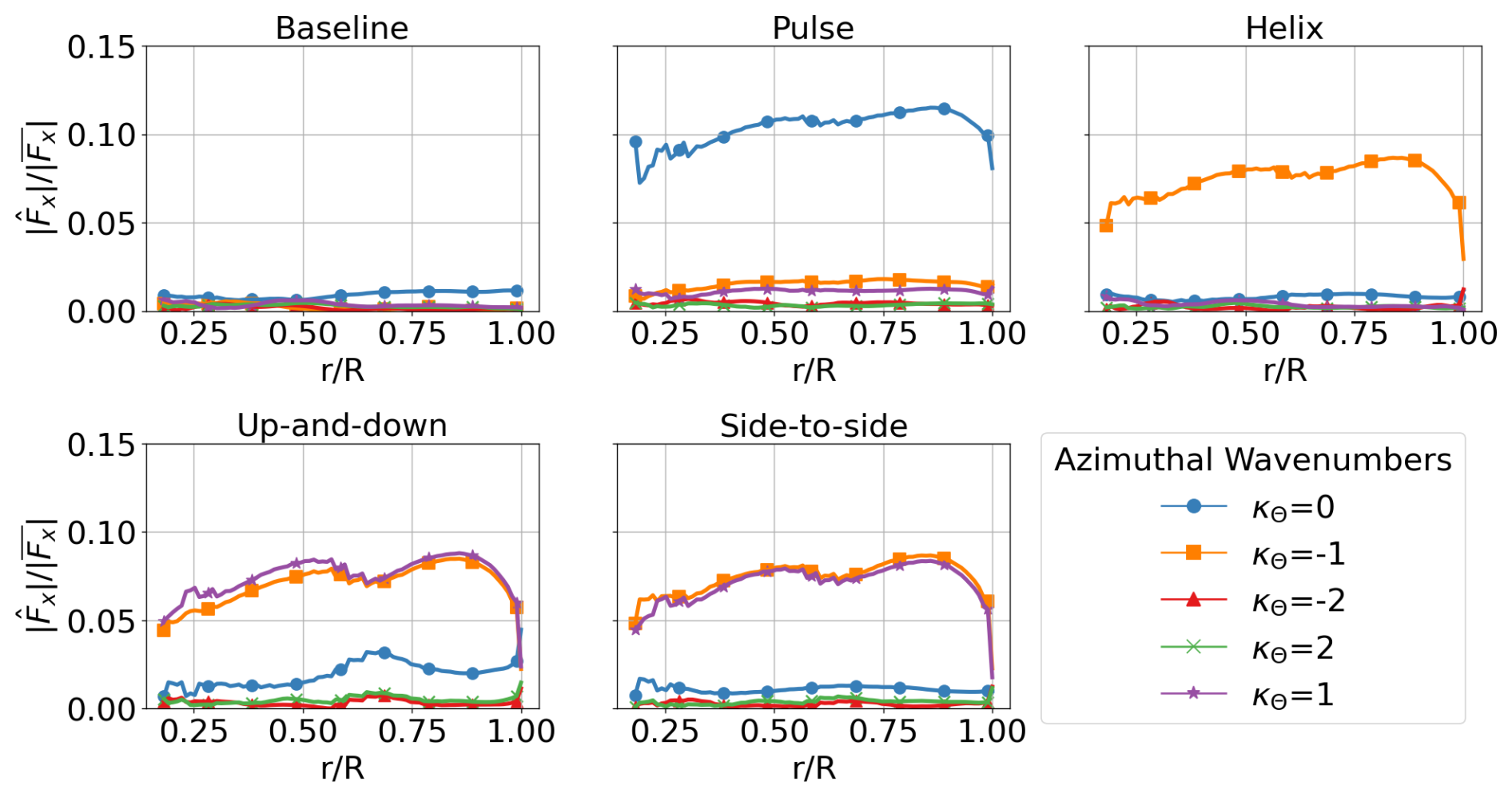
Figure 5 Variation in the axial blade loading for each AWM strategy. The individual curves correspond to the magnitude of the Fourier coefficients of the axial force $\left|{\widehat{F}}_x\right|$ at St=0.3 for different azimuthal wavenumbers κ_θ, normalized by the mean axial blade loading $\left|{\stackrel{\mathrm{‾}}{F}}_x\right|$.

To analyze the corresponding wavenumber and frequency content in the wake, a SPOD analysis is formulated in the following section.

2.2 SPOD formulation

Proper orthogonal decomposition (POD), also referred to as principle component analysis or Karhunen–Loéve decomposition, is a common data analysis technique that identifies a set of deterministic modes that optimally represent the energy in a stochastic process. Since its inception by Lumley (1967), several formulations of POD have emerged and been applied to a wide range of applications (Towne et al., 2018). In this paper, the focus is on spectral POD, which identifies the dominant coherent structures in a flow through a set of spatial–temporal modes (Picard and Delville, 2000). This differs from a space-only POD (Sirovich, 1987; Aubry et al., 1988; Ali et al., 2017) by considering the frequency content of the data, which is particularly useful in the context of AWM for tracking flow structures that are forced at specific Strouhal numbers. Additionally, a polar decomposition is used here to represent spatial correlations as in Citriniti and George (2000), and a Fourier transform is applied in the azimuthal direction so that velocity correlations in the radial direction r are considered at each azimuthal wavenumber κ_θ and frequency ω. This setup allows for the evolution of the forced azimuthal wavenumbers and frequencies that are input to the turbine controller to be explicitly tracked in the flow, as well as their interactions with other wake structures.

Given a time series of planar velocity field data, SPOD is defined by the eigenvalues and eigenvectors of the cross-spectral density tensor S, which is the time Fourier transform of the two-point space–time velocity correlation tensor (Towne et al., 2018). For a statistically stationary flow, the cross-spectral density tensor at a specific frequency ω and azimuthal wavenumber κ_θ can be expressed as $\mathbf{S}(r,r^{\prime })=\langle \widehat{\mathit{u}}(r,{\mathit{\kappa }}_{\mathit{\theta }},\mathit{\omega }){\widehat{\mathit{u}}}^{*}(r^{\prime },{\mathit{\kappa }}_{\mathit{\theta }},\mathit{\omega })\rangle$, where $\widehat{\mathit{u}}$ are the velocity Fourier coefficients, 〈  〉 is the expectation operator, and ^* represents the complex conjugate of a scalar or the Hermitian transpose of a tensor (Citriniti and George, 2000). In this paper, u denotes the fluctuating velocity field, since SPOD typically operates on a zero-mean stochastic process, and U will be used for the mean velocity field. The eigenvalue problem is then expressed as

$$\begin{array}{}\text{(3)}& \int \mathbf{S}(r,r^{\prime },{\mathit{\kappa }}_{\mathit{\theta }},\mathit{\omega })\mathit{\psi }(r^{\prime },{\mathit{\kappa }}_{\mathit{\theta }},\mathit{\omega })\mathrm{d}{r}^{\prime }=\mathit{\lambda }({\mathit{\kappa }}_{\mathit{\theta }},\mathit{\omega })\mathit{\psi }(r,{\mathit{\kappa }}_{\mathit{\theta }},\mathit{\omega }).\end{array}$$

The solution to Eq. (3) is a set of eigenvalues λ and orthogonal eigenvectors ψ. The eigenvectors represent individual flow structures, and the eigenvalues represent the average TKE of flow that is captured by the eigenvectors. Therefore, the eigenvalues can be used to rank the eigenvectors ${\mathit{\psi }}_{\mathrm{1}},{\mathit{\psi }}_{\mathrm{2}},{\mathit{\psi }}_{\mathrm{3}},\mathrm{\cdots }$ from most to least energetic across all κ_θ and ω, such that ${\mathit{\lambda }}_{\mathrm{1}}\ge {\mathit{\lambda }}_{\mathrm{2}}\ge \mathrm{\cdots }\ge \mathrm{0}$. In this sense, the velocity Fourier coefficients $\widehat{\mathit{u}}$ can be optimally expanded from the most energetic to the least energetic structures in the flow as

$$\begin{array}{}\text{(4)}& \widehat{\mathit{u}}(r,{\mathit{\kappa }}_{\mathit{\theta }},\mathit{\omega })=\sum _{j=\mathrm{1}}^{\mathrm{\infty }}{a}_j({\mathit{\kappa }}_{\mathit{\theta }},\mathit{\omega }){\mathit{\psi }}_j(r,{\mathit{\kappa }}_{\mathit{\theta }},\mathit{\omega }),\end{array}$$

where $a_j({\mathit{\kappa }}_{\mathit{\theta }},\mathit{\omega })=\int \widehat{\mathit{u}}(r,{\mathit{\kappa }}_{\mathit{\theta }},\mathit{\omega }){\mathit{\psi }}_j^{*}(r,{\mathit{\kappa }}_{\mathit{\theta }},\mathit{\omega })\mathrm{d}r$ is obtained by projecting the velocity Fourier coefficient onto the jth eigenvector. We can define ${\widehat{\mathit{u}}}_j(r,{\mathit{\kappa }}_{\mathit{\theta }},\mathit{\omega })\equiv a_j({\mathit{\kappa }}_{\mathit{\theta }},\mathit{\omega }){\mathit{\psi }}_j(r,{\mathit{\kappa }}_{\mathit{\theta }},\mathit{\omega })$ as the contribution to the velocity Fourier coefficients from the jth eigenvector. The real-space velocity field is recovered by performing an inverse Fourier transform in the temporal and azimuthal directions, i.e.

$$\begin{array}{}\text{(5)}& \begin{array}{rl}\mathit{u}(r,\mathit{\theta },t)& =\sum _{j=\mathrm{1}}^{\mathrm{\infty }}{\mathit{u}}_j(r,\mathit{\theta },t)\\ & =\sum _{j=\mathrm{1}}^{\mathrm{\infty }}\left[\int \int {\widehat{\mathit{u}}}_j(r,{\mathit{\kappa }}_{\mathit{\theta }},\mathit{\omega }){\mathrm{e}}^{\mathrm{i}({\mathit{\kappa }}_{\mathit{\theta }}\mathit{\theta }+\mathit{\omega }t)}\mathrm{d}{\mathit{\kappa }}_{\mathit{\theta }}\mathrm{d}\mathit{\omega }\right].\end{array}\end{array}$$

In Eq. (5), ${\mathit{u}}_j(r,\mathit{\theta },t)$ denotes the reconstruction of the velocity field in real space from the jth SPOD eigenvector. Similarly, the velocity can be reconstructed from the leading N eigenvectors by truncating the summations in Eqs. (4) and (5). More generally, we denote ${\mathit{u}}_{\mathcal{J}}={\sum }_{j\in \mathcal{J}}{\mathit{u}}_j(r,\mathit{\theta },t)$ as the reconstruction of the velocity field from a collection of eigenvectors defined by a given set of integers 𝒥. Further details on the general application of SPOD to fluid dynamics, including its connection to dynamic mode decomposition (DMD) and resolvent analysis, are provided by Towne et al. (2018).

Given the computational setup in Sect. 2, SPOD is performed on time series of cross-flow planes extracted from the LES at multiple streamwise locations ranging from $-\mathrm{5}\le (x-x_{\text{hub}})/D\le \mathrm{14}$ (see Fig. 6). These y–z planes are sampled at a spatial resolution consistent with the local grid resolution and a frequency of 2 Hz over the 1100 s of simulation time. Each planar time series is divided into 19 overlapping blocks of data (N_B=19), and the cross-spectral density is approximated from an ensemble average of these realizations for each temporal frequency using a windowed Fourier transform in time. The short-time FFT routine from the SciPy package (Virtanen et al., 2020) is used to perform the padded windowed Fourier transform in time, providing routines for both forward and inverse transforms, allowing the flow field to be reconstructed in real space to machine precision using Eq. (4). Each block of data corresponds to 128 s of simulation time, with a 64 s overlap between consecutive blocks. This configuration allows for the resolution of Strouhal numbers down to St=0.15 within each block. The SPOD parameters discussed here were primarily chosen to maximize the number of blocks over the 1100 s time interval, while also ensuring good temporal resolution of the forcing Strouhal number 0.3.

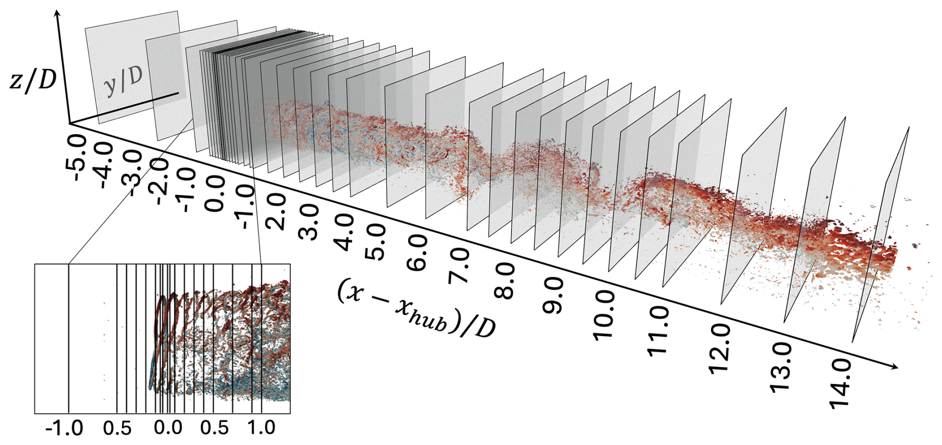
Figure 6 Schematic of the cross-flow planes used for the SPOD analysis. Isosurfaces of the baseline wake are also shown, colored by streamwise velocity. The cross-flow planes correspond to the streamwise locations: $(x-x_{\text{hub}})/D=-\mathrm{5.00}$, −2.50, −1.00, −0.50, −0.40, −0.30, −0.20, −0.10, −0.05, −0.025, 0.025, 0.05, 0.10, 0.20, 0.30, 0.40, 0.50, 0.70, 0.90, 1.0, 1.50, 2.0, 2.5, 3.0, 3.5, 4.0, 5.0, 6.0, 7.0, 7.5, 8.0, 8.5, 9.0, 9.5, 10.0, 10.50, 11.0, 12.0, 13.0, 14.0.

The velocity field is transformed to a polar grid with 256 uniformly spaced points in both the radial $r\in [\mathrm{0},L_R]$ and azimuthal $\mathit{\theta }\in [\mathrm{0},\mathrm{2}\mathit{\pi })$ directions. The radial extent of the flow region considered is taken to be L_R=1.4R, which brings the flow region to within a 1 m clearance from the ground at its lowest point. This radius is found to be sufficient for encompassing the wake near the turbine; however, the wake does spread anisotropically downstream beyond the extent of this radial domain (see Fig. 7a). Thus, only the wake dynamics within a 1.4R circular region are captured by the SPOD analysis here. This choice is made as the polar representation of the flow field is needed to track the flow structures at the specific azimuthal wavenumbers forced by the turbine controller. However, we note that SPOD could be applied to the full Cartesian data to analyze y–z correlations for the entire wake structure and that, while this would sacrifice the ability to examine specific wavenumbers, it would result in a more efficient basis for representing anisotropic structures in the wake.

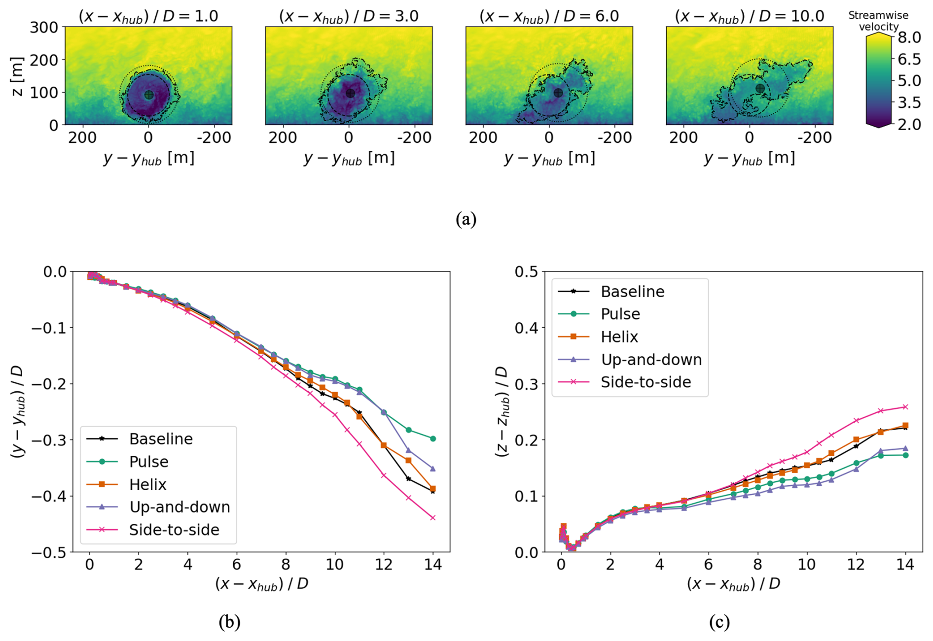
Figure 7 (a) Contours of streamwise velocity for the baseline case at $(x-x_{\text{hub}})/D=\mathrm{1}$, 3, 6, and 10. Dashed lines indicate the turbine rotor disk, dotted lines indicate a 1.4R disk around the wake centers, and dot-dashed lines indicate the wake boundaries identified using the SAMWICH package. The wake centers are also marked. Panels (b) and (c) show the mean lateral and vertical wake centers for each AWM case across the extent of the streamwise domain, respectively.

For each streamwise location in the wake, the polar coordinates are defined around the center of the wake, rather than a fixed y–z coordinate at all locations. This approach is taken because the turbulence in the wake, including the AWM-induced flow structures, will follow the mean movements of the wake, and we are interested in tracking their properties downstream. Further, the path that the actual wake travels dictates the worst-case position for a downstream turbine (and the best-case scenario for wake control), which further motivates the choice to use the wake position as the centering point for the analyses herein. The wake centers are identified by a velocity deficit weighted average over a $\mathit{\pi }{L}_R^{\mathrm{2}}$ area using the SAMWICH package (Quon et al., 2020) (see Fig. 7a). The lateral and vertical mean wake centers are shown in Fig. 7b and c, respectively, for each case in Table 1 across the extent of the streamwise domain. The mean wake generally moves up and to the right (when looking downstream), with the largest deviation from the hub height location occurring for the side-to-side actuation, which moves 0.45 D to the right and 0.26 D upward. The wake movement and skewness align with the direction of veer in the ABL. The polar transformation for each AWM case is defined around the wake center for the baseline case. This adjusts the analysis for wake movements as a result of the unsteady inflow to follow the general movement of the dominant flow structures but preserves differences in the induced wake movement from the baseline as a result of AWM. Subtraction of the wake centers also adjusts for wake expansion and veer due to mean flow effects. For all streamwise locations upstream of the turbine, the polar representation of the velocity field is centered on the turbine hub height.

All three cylindrical velocity field components, $\mathit{u}=(u_x,u_r,u_{\mathit{\theta }})$, are included in the SPOD analysis of the cross-spectral density tensor. This approach provides the most comprehensive description of the coherent structures in the flow because it contains correlations between all components of the velocity field. However, the eigenvalues and eigenvectors of the components of the trace of S can also be used to identify the response of each velocity component to AWM individually (see Appendix A). In this case, S₁₁, S₂₂, and S₃₃ are identified with the streamwise, radial, and azimuthal velocity components, respectively. This is useful for discerning which components of the flow are contributing the most TKE to a given flow structure. For both S and its diagonal elements, the discrete eigenvalue problem is solved using a low-rank SVD solver, which results in N_B eigenvalues and eigenvectors for each κ_θ and ω. More details on the solution to the discrete eigenvalue problem are provided in Appendix B.

3 Results

In this section, the wake mixing dynamics and efficacy of each AWM strategy are explored through the SPOD analysis. The energetic flow structures are tracked throughout the wake in Sect. 3.1 and connected to turbulent entrainment statistics in Sect. 3.2. The practical benefits of AWM are also demonstrated for a two-turbine array in Sect. 3.3.

3.1 SPOD results

The SPOD eigenvalues are used to track the dominant flow structures throughout the streamwise domain. The results primarily focus on the azimuthal wavenumbers κ_θ=0, ±1 and ±2 at St=0.3 as this range encompasses the forced coherent structures for each AWM case, as well as other large-scale structures that get excited downstream in the wake. The eigenvalues for the baseline case are also analyzed at these wavenumbers for a wider range of frequencies (Fig. 8), which represent the energy in the inherent flow structures in the non-actuated wake resulting from standard turbine operations. Both the absolute values of the eigenvalues (Fig. 9) and the baseline normalized eigenvalues (Fig. 10) are discussed, which quantify the dominant coherent structures in the wake for each control strategy and the effectiveness of AWM at exciting structures in the wake over the baseline, respectively. Comparisons in the modal behavior for each AWM case offer insights into their relative performance, which are further strengthened in Sect. 3.2 and 3.3. In addition to eigenvalues, the reconstruction of the velocity field from the leading SPOD eigenvectors is used to show the leading flow structures in the wake and the induction field.

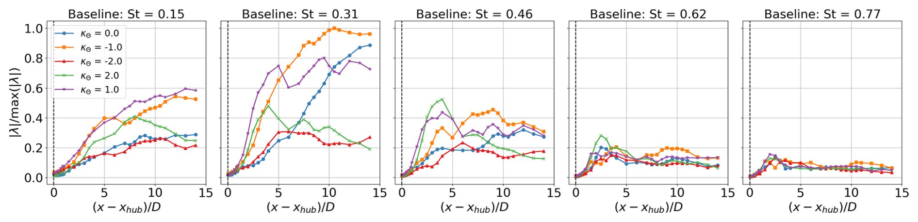
Figure 8 Eigenvalues of S at five different Strouhal numbers for the baseline case. Shown are the azimuthal wavenumbers κ_θ=0, ±1, and ±2. Each eigenvalue is normalized by the global maximum baseline eigenvalue across all streamwise locations and Strouhal numbers.

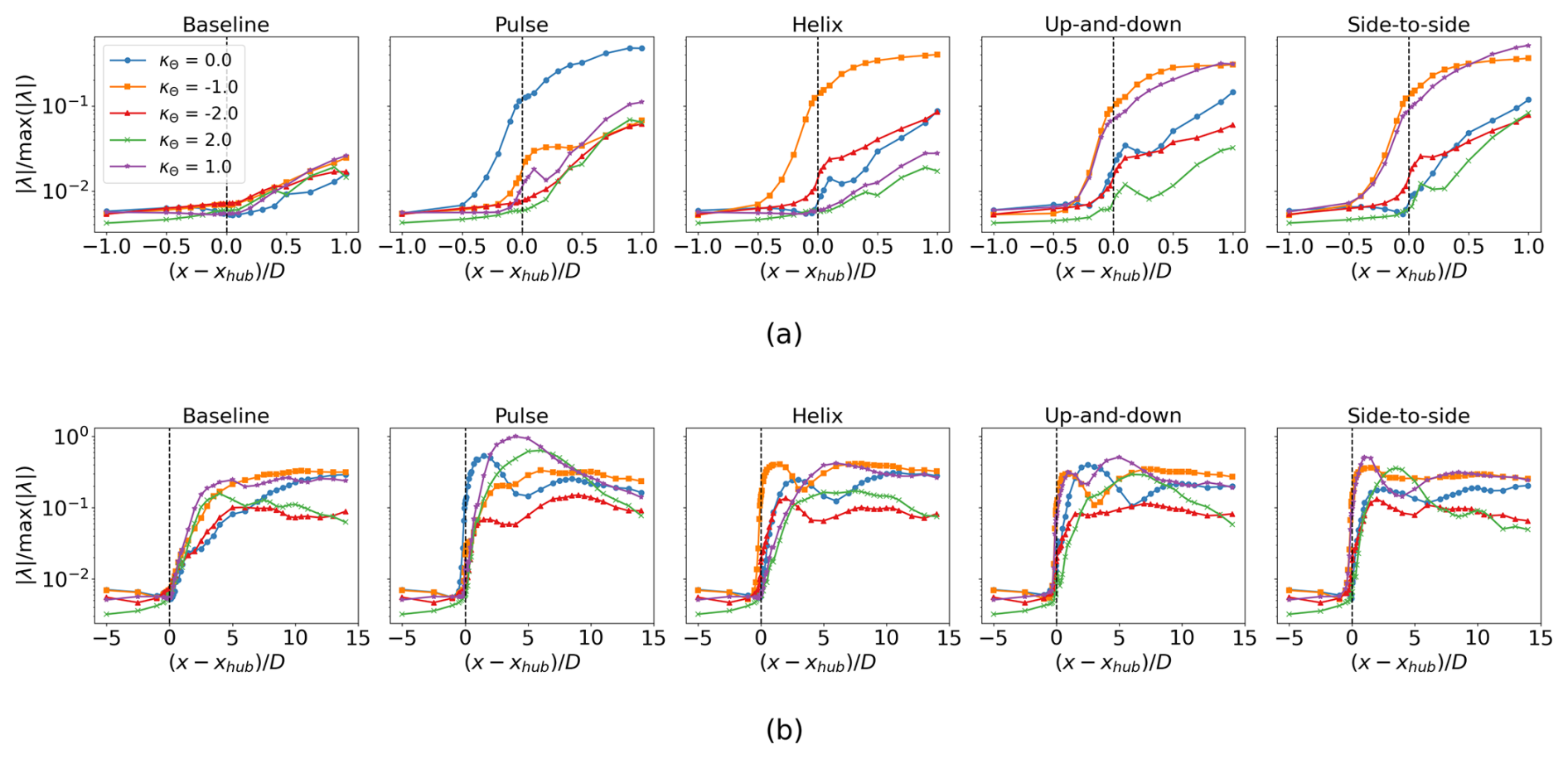
Figure 9 Eigenvalues of S at St=0.3 for the azimuthal wavenumbers κ_θ=0, ±1, and ±2. Each eigenvalue is normalized by the global maximum eigenvalue across all AWM cases and streamwise locations. The eigenvalues are shown near the turbine region ($\left|\right(x-x_{\text{hub}})/D|\le \mathrm{1}$) in the top row of figures (a) and across the entire streamwise domain $-\mathrm{5}\le (x-x_{\text{hub}})/D\le \mathrm{14}$ in the bottom row of figures (b).

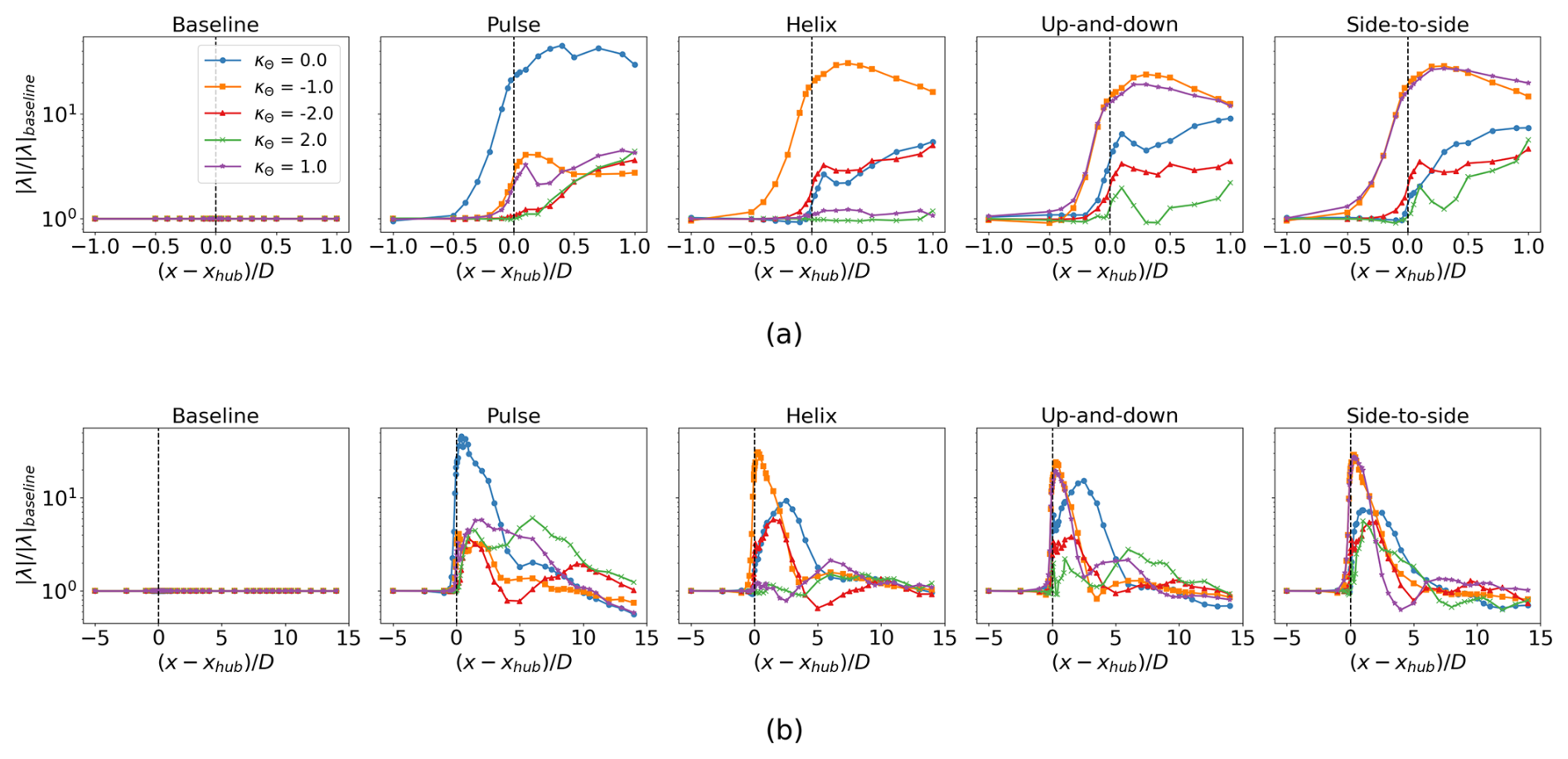
Figure 10 Baseline normalized eigenvalues of S at St=0.3 for the azimuthal wavenumbers κ_θ=0, ±1, and ±2. The eigenvalues for each wavenumber and streamwise location are normalized by the corresponding eigenvalues in the baseline case. The eigenvalues are shown near the turbine region ($\left|\right(x-x_{\text{hub}})/D|\le \mathrm{1}$) in the top row of figures (a) and across the entire streamwise domain $-\mathrm{5}\le (x-x_{\text{hub}})/D\le \mathrm{14}$ in the bottom row of figures (b).

In Fig. 8, the eigenvalues for the baseline wake are shown for a broad frequency range. In general, the most energetic structures in the wake are found at St=0.3, which may explain the effectiveness of AWM forcing frequencies near this value (Munters and Meyers, 2018; Cheung et al., 2024; Brown et al., 2025; Frederik et al., 2020c, 2025). In this sense, SPOD could provide a way to identify the optimal AWM forcing frequency based on baseline wake data. A more detailed investigation of the baseline wake within the range $\mathit{\text{St}}\in [\mathrm{0.25},\mathrm{0.35}]$ would be worthwhile for future research; however, the SPOD parameters selected in this study do not permit such fine resolution. There is also considerable energy present in the baseline wake at St=0.15, suggesting potential support for sub-harmonic forcing strategies (Li et al., 2024). In contrast, the energy content at higher Strouhal numbers (St>0.6) is largely insignificant when compared to lower values. The remainder of this section focuses on St=0.3, as this corresponds to the dominant frequency in the baseline wake and the AWM forcing frequency that was selected a priori.

In the baseline case, a small distinction between large-scale flow structures at St=0.3 originates in the induction field ahead of the turbine, which grows significantly in the wake (see Fig. 9). The ${\mathit{\kappa }}_{\mathit{\theta }}=-\mathrm{1}$ mode is the dominant flow structure in the immediate near wake of the turbine as well as in the far wake, while the κ_θ=1 mode is the leading structure between 0.5 D and 5 D downstream of the turbine. Together, the ±1 modes result in a mean movement of the wake, as well as a swirl component if the energy in these modes is imbalanced. SPOD decouples these competing rotational effects in the wake, allowing them to be examined independently. There are several factors contributing to the swirl of the baseline wake. The clockwise rotation of the turbine blades, for instance, imparts a counter-clockwise swirl in the mean wake, which may be contributing to the large ${\mathit{\kappa }}_{\mathit{\theta }}=-\mathrm{1}$ mode. Similarly, the positive veer in this ABL introduces a horizontal shear to the wake, resulting in a large-scale counter-clockwise swirl, which may be contributing to the κ_θ=1 mode. Other prominent energetic structures in the baseline wake include the κ_θ=2 mode in the near-wake region and the κ_θ=0 mode in the far wake.

For each AWM case, the largest increase in eigenvalues over the baseline occurs in the near-wake region between 0.25 D and 1 D behind the turbine, corresponding to the azimuthal wavenumber directly forced by the dynamic blade pitch settings, i.e. κ_θ=0 for the pulse, ${\mathit{\kappa }}_{\mathit{\theta }}=-\mathrm{1}$ for the helix, and ${\mathit{\kappa }}_{\mathit{\theta }}=\pm \mathrm{1}$ for the up-and-down and side-to-side actuations (see Fig. 10). The SPOD analysis therefore confirms that the azimuthal wavenumber and frequency inputs to the turbine controller lead to the intended flow response directly downstream of the turbine. The streamwise velocity component contributes the most to the TKE of the coherent structures in the near-wake region, although a similar modal response is induced in the radial and azimuthal components (see Appendix A). This is expected as the most observable effect of the blade pitch fluctuations is on the axial loading. It is also readily apparent from the leading SPOD mode shapes that the intended flow perturbations are imparted on the wake for each AWM case (see Fig. 11a). The primary flow perturbation in the near wake for the pulse actuation is axisymmetric and oscillates at the Strouhal period. The coherent structures for the other AWM strategies are characterized by two regions of low- and high-speed flow, which rotate about the wake center for the helix case and oscillate at the Strouhal period for the mixed-mode forcings depending on the clocking angle. To connect the SPOD eigenvectors to more familiar flow quantities, we note that these flow patterns can also be observed in the region near the rotor by carefully phase averaging the real-space flow. In Fig. 12, the phase-averaged baseline-subtracted velocity field is shown for each AWM case. The leading SPOD modes are clearly apparent in the phase-averaged fields, demonstrating that the flow patterns identified by SPOD are indeed the dominant coherent structures in the wake.

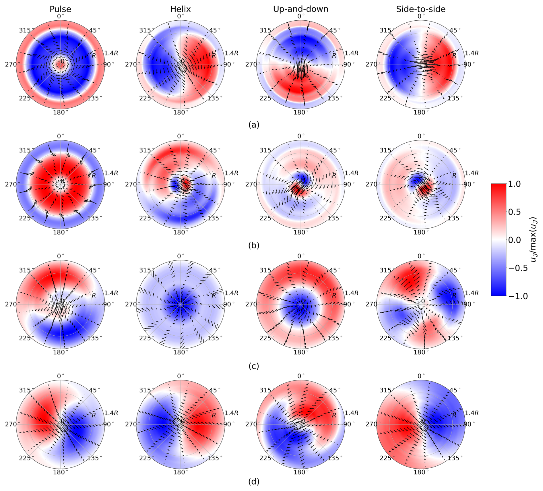
Figure 11 Dominant flow structures at four streamwise locations in the wake: (a) $(x-x_{\text{hub}})/D=\mathrm{0.1}$, (b) $(x-x_{\text{hub}})/D=\mathrm{1.0}$, (c) $(x-x_{\text{hub}})/D=\mathrm{3.0}$, and (d) $(x-x_{\text{hub}})/D=\mathrm{6.0}$. The reconstructed fluctuating velocity field u_𝒥(r,θ) is shown at a single instance in time using the SPOD eigenvectors that correspond to the leading eigenvalues for St=0.3. For each case, the reconstructed velocity field is normalized by its maximum value in the polar domain at that specific time. For the pulse and helix cases, one SPOD mode is included in the reconstruction, i.e. $\mathcal{J}=\mathit{\left\{}\mathrm{1}\right|\mathit{\omega }{U}_{\text{inf}}/D=\mathrm{0.3}\mathit{\}}$. For the up-and-down and side-to-side cases, two SPOD modes are included in the flow reconstruction, i.e. $\mathcal{J}=\mathit{\{}\mathrm{1},\mathrm{2}|\mathit{\omega }{U}_{\text{inf}}/D=\mathrm{0.3}\mathit{\}}$. The colored contours show normalized streamwise velocity, and the arrows denote the in-plane velocities.

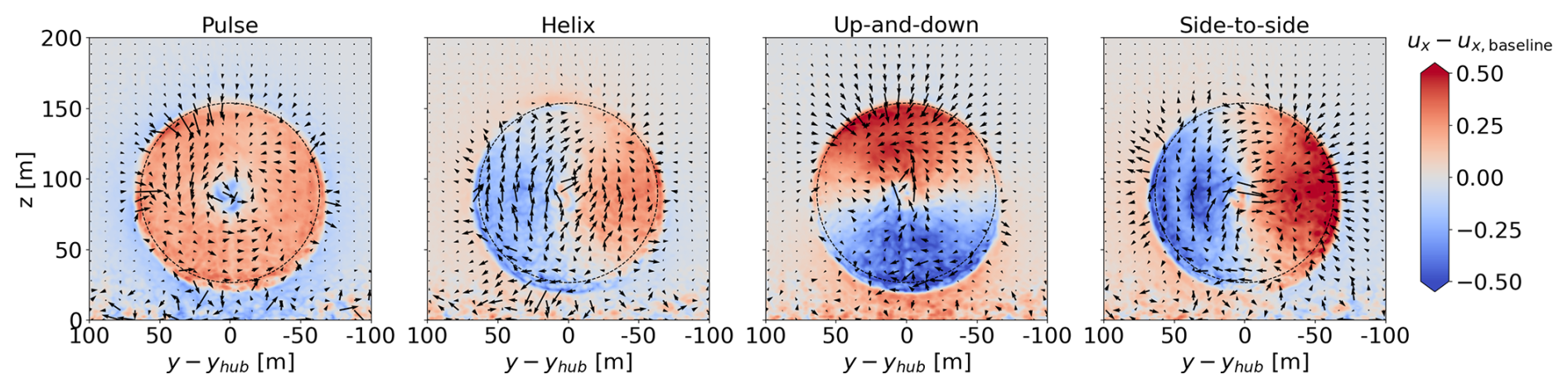
Figure 12 Phase-averaged baseline-subtracted velocity fields at $(x-x_{\text{hub}})/D=\mathrm{0.1}$. Phase averaging in the Strouhal cycle is performed with a 10° bin centered on 0°. After the phase averaging is performed for all cases, both the streamwise and lateral components of velocity are baseline subtracted to yield the colored contours and the vector fields, respectively. The dashed lines outline the turbine rotor disk.

The eigenvalues of the forced azimuthal wavenumber(s) begin to increase from the baseline values around 0.5 D upstream of the turbine for each AWM strategy and grow rapidly through the induction field to reach a value over an order of magnitude larger than the baseline at the turbine location (see Fig. 10). AWM therefore modifies the induction field with similar spectral characteristics as those imparted on the wake region directly behind the turbine. However, unlike in the wake, the coherent structures at St=0.3 are not the dominant energy-containing modes in the induction field, which instead occur near the blade-passing frequency (St≈7.5) for each AWM case (see Fig. 13a). Nonetheless, SPOD allows these structures to be decoupled, and the focus here is on modes at the excitation frequency (Fig. 13b). The azimuthal and temporal modifications to the turbine induction field translate to variations in the axial force along the blade (compare Figs. 5 and 9a), which are subsequently imparted to the downstream wake. Notably, the κ_θ=0 in the near-wake region of the pulse case exhibits a larger increase in energy over the baseline compared to the forced wavenumbers associated with the other AWM strategies. This observation aligns with the larger variations in blade loading seen with the pulse method compared to the other cases. The structure of the dominant modes in the induction field may provide insight into why there is increased blade loading observed with pulse actuation relative to the other AWM strategies. For the non-axisymmetric forcings, the in-plane velocity field in the induction zone is seen to divert the flow from the low- to high-speed region of the streamwise velocity (see Fig. 13b). This suggests that the individual pitching of the turbine blades creates a non-uniform blockage in the flow, leading to flow diversion around the region of higher blockage, consequently reducing the periodic axial blade force that actuates the wake modes. However, in the pulse case, there is no apparent flow diversion because all the blades are collectively pitched. This increase in blade loading for the pulse case is seemingly important as it translates to the largest modal energy in the near-wake region which, as discussed further in Sect. 3.2, facilitates the most effective mixing of the downstream wake.

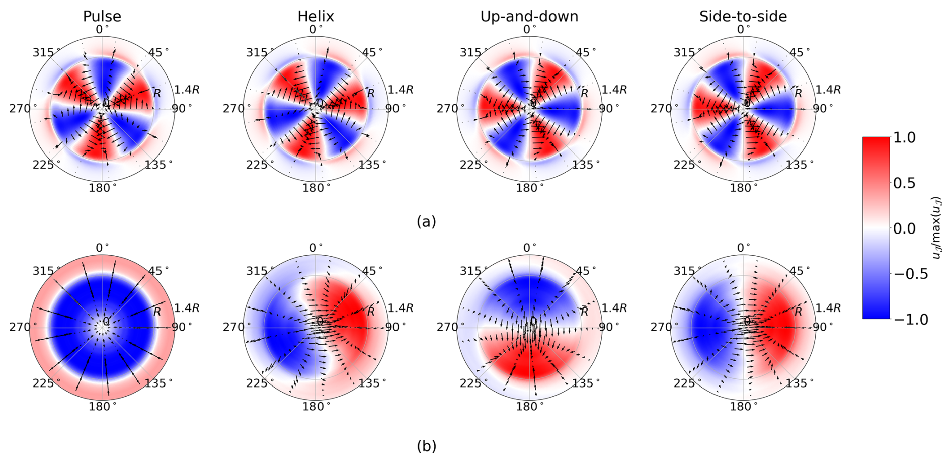
Figure 13 Flow structures in the induction field at $(x-x_{\text{hub}})/D=-\mathrm{0.1}$. The reconstructed fluctuating velocity field ${\mathit{u}}_{\mathcal{J}}(r,\mathit{\theta },t)$ is shown at a single instance in time. For each case, the reconstructed velocity field is normalized by its maximum value in the polar domain at that specific time. For the pulse and helix case, one SPOD mode is included in the reconstruction, whereas for the up-and-down and side-to-side cases, two SPOD modes are included in the flow reconstruction. In panel (a), the leading SPOD eigenvectors across all wavenumbers and frequencies are used, i.e. 𝒥={1} for the pulse and helix methods and $\mathcal{J}=\mathit{\{}\mathrm{1},\mathrm{2}\mathit{\}}$ for the up-and-down and side-to-side methods. In panel (b), the leading SPOD eigenvectors across all wavenumbers at St=0.3 are used, i.e. $\mathcal{J}=\mathit{\left\{}\mathrm{1}\right|\mathit{\omega }{U}_{\text{inf}}/D=\mathrm{0.3}\mathit{\}}$ for the pulse and helix method and $\mathcal{J}=\mathit{\{}\mathrm{1},\mathrm{2}|\mathit{\omega }{U}_{\text{inf}}/D=\mathrm{0.3}\mathit{\}}$ for the up-and-down and side-to-side method. The colored contours show the normalized streamwise velocity, and the arrows denote the in-plane velocities.

As the wake evolves downstream, non-linear and mean flow interactions excite flow structures beyond those directly forced by the turbine controller. For the non-axisymmetric forcing strategies, there is a notable increase in the κ_θ=0 wavenumber relative to the baseline between $\mathrm{2}\le (x-x_{\text{hub}})/D\le \mathrm{5}$, which dominates the baseline normalized eigenvalues in this region (Fig. 10b). For the pulse case, the increase over the baseline is sustained by the κ_θ=1 and 2 wavenumbers between $\mathrm{3}\le (x-x_{\text{hub}})/D\le \mathrm{10}$. By 10 D to 14 D downstream, the ${\mathit{\kappa }}_{\mathit{\theta }}=-\mathrm{1}$ mode is dominant in all cases, but the modal energy in the large scales has generally returned to the baseline levels for all of the AWM strategies. However, we note that increases in pitching amplitude or adjustments to the Strouhal number may extend the duration of AWM effects. Moreover, it is important to highlight that, although the modal energy relative to the baseline wake generally decreases downstream for the AWM cases, the modal energy in the baseline wake itself typically increases downstream (Fig. 9b). Consequently, the flow structure with the largest modal energy for the AWM cases may not be located in the immediate near wake of the turbine, despite the largest increases over the baseline occurring in that region. It is clear from the SPOD modes, for instance, that the dominant flow structure, in terms of the absolute magnitude of the eigenvalues, changes as the wake evolves downstream (see Fig. 11b–d). The largest absolute eigenvalue across all AWM cases and streamwise locations occurs for the κ_θ=1 wavenumbers for the pulse actuation 4 D downstream (see Fig. 9b). In fact, for all AWM cases, the largest eigenvalues between 5 and 6 D downstream is for the κ_θ=1 wavenumber. The energy in this mode is primarily driven by the radial velocity component u_r, which is generally true of the modal energy increases over the baseline by 4 D to 5 D downstream (see Appendix A). Notably, the κ_θ=1 mode is also the dominant structure in the near-wake region of the baseline case, which suggests that the effectiveness of AWM strategies at increasing modal energy in the wake is related to their ability to excite the natural flow structures in the non-actuated wake. This appears to be the case for higher harmonics in the flow as well, such as the κ_θ=2 mode for the pulse and side-to-side actuations (see Fig. 9b).

The flow response in the wake between the two mixed-mode forcing strategies differs significantly even though both strategies excite the ${\mathit{\kappa }}_{\mathit{\theta }}=\pm \mathrm{1}$ modes. This behavior highlights the fact that differences in the clocking angle cause flow structures to interact differently with the ABL, including variations in shear, stratification, turbulence, and ground effect. By 3 D to 6 D downstream, the up-and-down strategy strongly forces the κ_θ=0 and 1 modes, while the side-to-side strategy forces the κ_θ=2 mode (Fig. 9b). Interestingly, the κ_θ=1 and −1 modes have nearly identical growth rates in the induction field ahead of the turbine for these cases, but, directly behind the turbine, ${\mathit{\kappa }}_{\mathit{\theta }}=-\mathrm{1}$ emerges as the dominant flow structure for both cases. This suggests that the ${\mathit{\kappa }}_{\mathit{\theta }}=-\mathrm{1}$ mode is enhanced by the counter-clockwise vortex rings generated behind the turbine, which have also been linked to the performance differences between the counter-clockwise and clockwise helix strategies (Coquelet et al., 2024).

The total resolved TKE in the wake at each streamwise location can be computed by summing the entire set of eigenvalues across all wavenumbers and frequencies (see Fig. 14). In the near wake, the up-and-down and side-to-side forcings have the largest TKE increase over the baseline, because two modes are forced at the same pitching amplitude as opposed to the single modes in the pulse and helix case. However, by 3 D downstream, the increase in TKE over the baseline drops to around 10 % for the non-axisymmetric forcings, while the pulse case maintains around a 15 %–20 % increase until 9 D downstream. This increase for the pulse actuation is driven by TKE in the radial velocity (see S₂₂ in Fig. 14). It is important to note that the goal of AWM is to increase TKE in the large-scale coherent structures of the wake that entrain the freestream momentum, not necessarily to increase wake TKE in general, which can impact blade loading on downstream turbines. To understand the separation of scales in the wake, the streamwise evolution of the eigenvalue spectra is reported in Fig. 15. In the pulse and helix cases, an order of magnitude decrease in the eigenvalue spectrum is observed after the first three SPOD modes at 0.5 D downstream. In contrast, the side-to-side and up-and-down cases exhibit a more gradual decay, attributed to the forcing of two modes by the blade pitch actuations, resulting in an order of magnitude decrease after six SPOD modes. This suggests that the flow is effectively represented by the leading SPOD modes in the near-wake region, where large-scale coherent structures dominate the flow's unsteadiness and account for the majority of the wake TKE. However, the decay becomes more gradual starting around 3 D downstream, and by 10 D, the distribution of modal energy across all AWM cases is similar to the turbulence in the baseline wake.

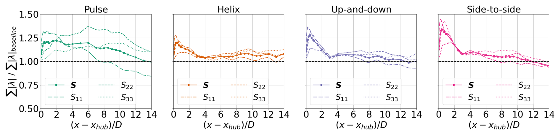
Figure 14 Baseline normalized TKE in the wake computed as the sum of the magnitude of eigenvalues of S across all wavenumbers and frequencies. The baseline normalized contribution to TKE from the streamwise, radial, and azimuthal velocity components is also shown and computed from the eigenvalues of S₁₁, S₂₂, and S₃₃, respectively.

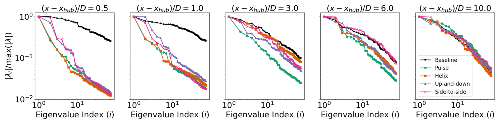
Figure 15 The eigenvalue spectra for each AWM strategy are shown at five streamwise locations in the wake. The leading 75 eigenvalues across all azimuthal wavenumbers and frequencies are included. Each spectrum is normalized by its leading eigenvalue $\left|{\mathit{\lambda }}_{\mathrm{1}}\right|$ to emphasize the relative decay in eigenvalues between cases.

3.2 Wake mixing and turbulent entrainment dynamics

The practical benefit of increased modal energy in the wake is additional entrainment of mean momentum by the coherent wake structures. This is the primary mechanism by which AWM enhances wake recovery and where the advantage of AWM lies over other wind farm control strategies. Entrainment is quantified here using the negative radial shear stress flux $\mathcal{T}=-U_x\stackrel{\mathrm{‾}}{u_x{u}_r}$, where $\stackrel{\mathrm{‾}}{\cdot }$ denotes the time average of a fluctuating quantity. This term quantifies the radial turbulent transport of mean streamwise kinetic energy, which Lebron et al. (2012) demonstrated is the dominant contributor to wake recovery for a single isolated turbine wake. Positive values of 𝒯 indicate a gain of mean flow into the wake due to turbulent transport, whereas the negative values of 𝒯 indicate a loss of mean flow.

The radial shear stress flux of the wake for the baseline case is shown in Fig. 16. Mean flow is primarily entrained through the boundary of the wake, which aligns with the rotor disk in the near-wake region but deforms anisotropically downstream. Veer, in particular, skews the wake significantly downstream, which in turn affects the distribution of 𝒯. A scalar measure of mean flow entrainment $\mathit{\tau }=\frac{\mathrm{1}}{\mathrm{2}\mathit{\pi }}{\int }_{\mathrm{0}}^{\mathrm{2}\mathit{\pi }}\mathcal{T}(r=D/\mathrm{2},\mathit{\theta })\mathrm{d}\mathit{\theta }$ is obtained by azimuthally averaging 𝒯 around the circumference of a rotor disk centered on the wake (see Fig. 17a). Wake recovery mechanisms are analyzed here in terms of a rotor disk centered around the wake centers at each streamwise location to track the entrainment properties of the wake structures downstream. This formulation is consistent with the SPOD analysis, which is computed around the wake centers.

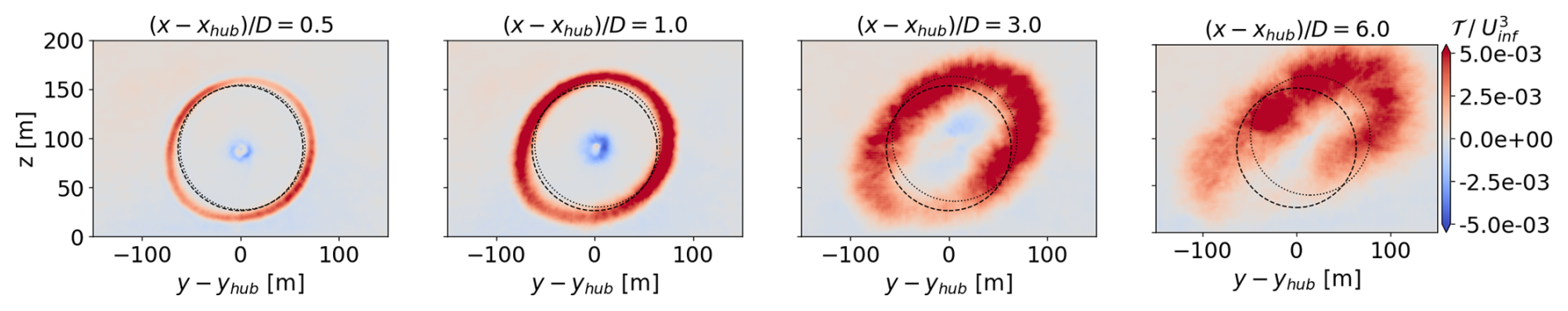
Figure 16 Contours of the radial shear stress flux 𝒯 for the baseline case at four different streamwise locations. The dashed line corresponds to the rotor disk centered at the hub height location, and the dotted line corresponds to the rotor disk centered around the wake centers.

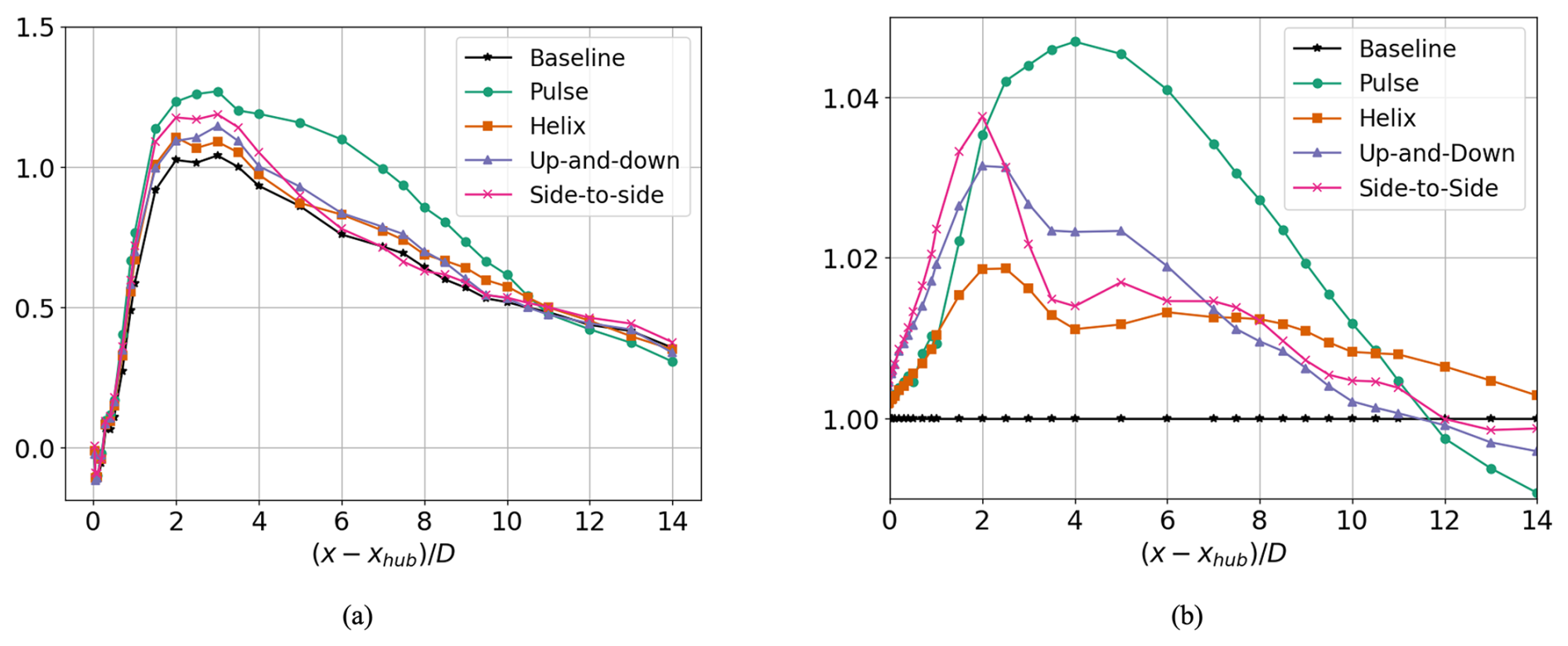
Figure 17 (a) Circumferential average of the radial shear stress flux around a rotor disk centered around the wake center, defined as $\mathit{\tau }=\frac{\mathrm{1}}{\mathrm{2}\mathit{\pi }}{\int }_{\mathrm{0}}^{\mathrm{2}\mathit{\pi }}\mathcal{T}(r=D/\mathrm{2},\mathit{\theta })\mathrm{d}\mathit{\theta }$. (b) Rotor-averaged velocity for each AWM case, normalized by the baseline value. The velocity is averaged over a rotor disk centered around the wake center.

All AWM strategies improve the net radial shear stress flux over the baseline throughout most of the streamwise domain, with the largest increases occurring between 2 D and 4 D behind the turbine (see Fig. 17a). Notably, the largest increase in the net mean flow entrainment is for the pulse actuation, which sustains an increase over the baseline between 3 D and 10 D downstream, whereas the other AWM cases return to the baseline levels in this region. This behavior is similar to the downstream evolution of the eigenvalues for the pulse case, which also sustained an increase over the baseline in this region. The improvement in radial shear stress flux over the baseline is not homogeneous around the rotor disk, however, and there are points where mean flow is even lost compared to the baseline due to the AWM pitch actuation (see Fig. 18). This is a departure from the canonical case analyzed by Cheung et al. (2024), further highlighting the impact of ABL characteristics on wake mixing dynamics, including wind veer, shear, and stratification. Moreover, the modal structure of the forcing is visible in the contours of 𝒯 within a turbine diameter downstream, where positive values are approximately axisymmetric for the pulse case but depend on the clocking angle for the up-and-down and side-to-side actuations.

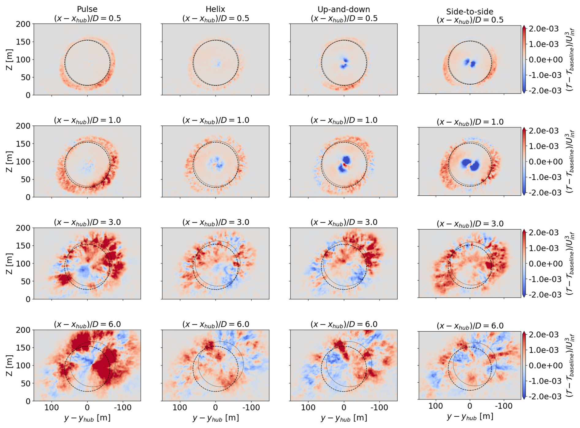
Figure 18 Contours of the baseline-subtracted radial shear stress flux for each AWM case. The dashed line corresponds to the rotor disk centered at the hub height location, and the dotted line corresponds to the rotor disk centered around the wake centers.

While Fig. 17a provides an overview of the total radial shear stress flux, SPOD facilitates a more detailed analysis of the contributions to this flux. The contribution from each flow structure in the wake to turbulent entrainment can be quantified by decomposing the radial shear stress flux into SPOD modes. Specifically, we can define the contribution to 𝒯 from the jth SPOD eigenvectors as

$$\begin{array}{}\text{(6)}& {\displaystyle }{\displaystyle }{\mathcal{T}}_{j,j}(r,\mathit{\theta })=-U_x\stackrel{\mathrm{‾}}{u_{x,j}{u}_{r,j}},\end{array}$$

where u_x,j and u_r,j are the streamwise and radial components of u_j. A full decomposition of 𝒯 is obtained by considering streamwise and radial velocity correlations between all pairs of SPOD eigenvectors, namely ${\mathcal{T}}_{j,k}(r,\mathit{\theta })=-U_x\stackrel{\mathrm{‾}}{u_{x,j}{u}_{r,k}}$. However, the focus here is on the case when j=k, which is found to dominate 𝒯_j,k for all wavenumbers and frequencies of interest. This is expected as the AWM forcings induce a similar modal response in the streamwise and radial velocity components (see Appendix A). Similarly to 𝒯, the net mean flow entrainment into the rotor disk from 𝒯_j,j can be quantified by the scalar measure ${\mathit{\tau }}_{j,j}=\frac{\mathrm{1}}{\mathrm{2}\mathit{\pi }}{\int }_{\mathrm{0}}^{\mathrm{2}\mathit{\pi }}{\mathcal{T}}_{j,j}(r=D/\mathrm{2},\mathit{\theta })\mathrm{d}\mathit{\theta }$. While the eigenvalue $\left|{\mathit{\lambda }}_j\right|$ is a scalar measure of modal TKE, the scalar quantity τ_j,j represents the contributions to the net radial shear stress flux from the jth SPOD mode. The quantity τ_j,j is positive for any mode that leads to a net turbulent entrainment of mean velocity into the wake and negative for modes leading to the entrainment of mean velocity out of the wake.

The decomposition of 𝒯 into SPOD modes enables a quantitative comparison between the modal contributions to turbulent entrainment, τ_j,j, and modal TKE, $\left|{\mathit{\lambda }}_j\right|$, in the wake (see Fig. 19). For each AWM case, the wavenumbers directly forced by the blade pitch actuations entrain the most momentum directly behind the turbine; however, this is not necessarily the case throughout the entire wake. Turbulent entrainment for the pulse actuation at St=0.3 is driven by the κ_θ=1 and 2 wavenumbers between 3 D and 10 D downstream, explaining the large aforementioned increase in τ over the baseline for the pulse case in this region. However, the contribution from the κ_θ=0 mode drops below that of the baseline for the pulse case by 4 D downstream. The κ_θ=1 and 2 wavenumbers are the dominant flow structures in the near wake of the baseline case, in terms of both TKE and entrainment, which suggests that optimizing AWM depends on forcing the natural coherent structures in the non-actuated wake, either directly through the turbine controller or indirectly through triadic wavenumber interactions (Waleffe, 1992) in the wake and interactions with other ABL processes. Similarly, the κ_θ=1 and 2 modes contribute significantly to entrainment for both mixed-mode forcing strategies; however, their entrainment characteristics in the wake differ. In the up-and-down case, the κ_θ=1 and 2 modes contribute the most to entrainment between 4 D and 10 D downstream following the excitation of the 0 mode in the near-wake region. In contrast, for the side-to-side case, the κ_θ=2 mode entrains the most momentum in the near wake while the 1 mode dominates in the far wake. Finally, even though the counter-clockwise helix method is used here to excite the ${\mathit{\kappa }}_{\mathit{\theta }}=-\mathrm{1}$ mode, the largest contribution to entrainment in the wake is from the κ_θ=1 mode between 5 D and 7 D downstream.

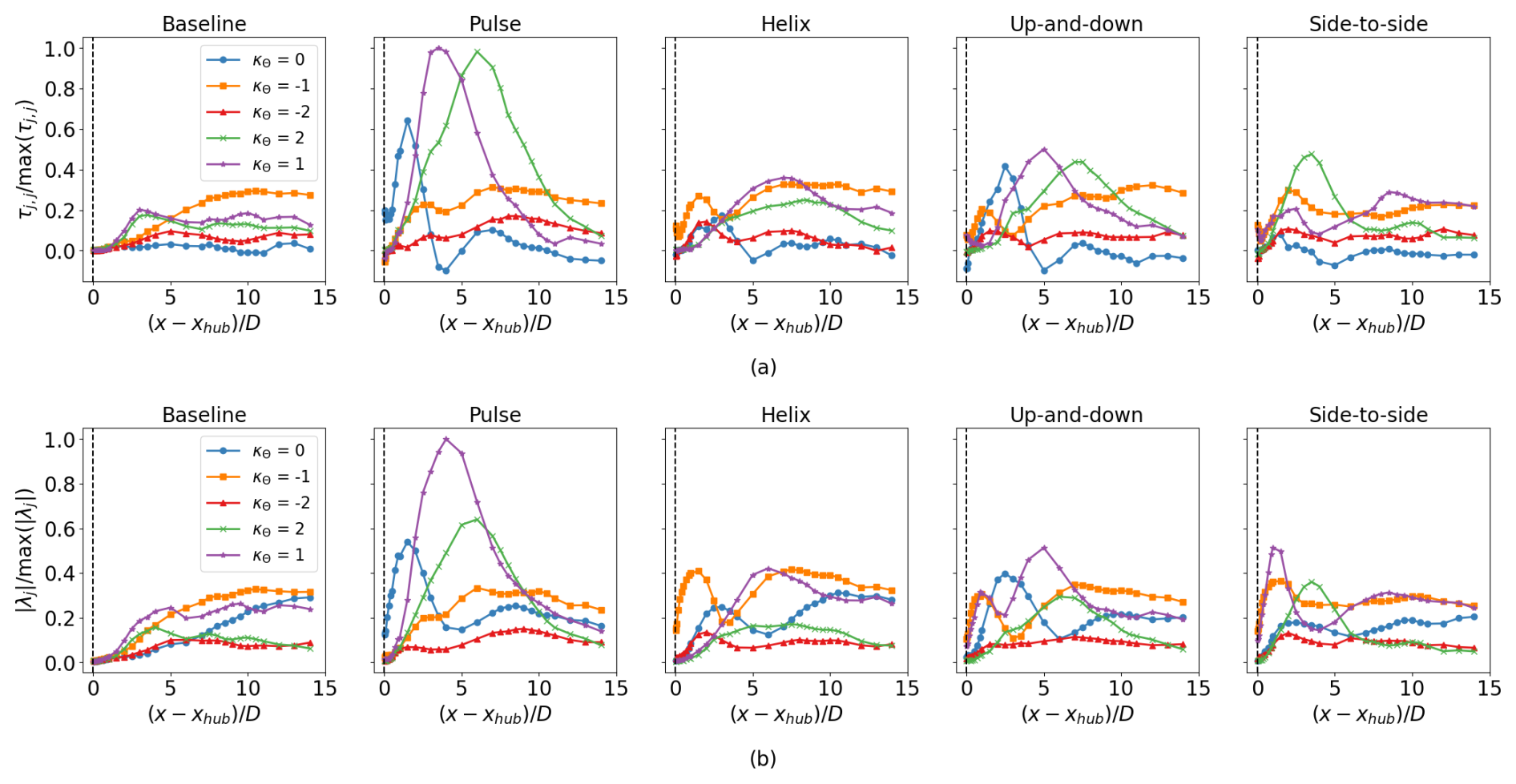
Figure 19 Modal contributions to (a) entrainment and (b) TKE in the wake, which is quantified by the (a) azimuthally averaged contributions to the radial shear stress flux τ_j,j and (b) the eigenvalues $\left|{\mathit{\lambda }}_j\right|$ from the leading SPOD eigenvectors at St=0.3 and ${\mathit{\kappa }}_{\mathit{\theta }}=\mathrm{0},\pm \mathrm{1},$ and ±2. Each AWM case is shown in addition to the baseline. The values in (a) and (b) are normalized by the maximum values of τ_j,j and $\left|{\mathit{\lambda }}_j\right|$ across all AWM strategies and streamwise locations, respectively.

Given the prominence of the κ_θ=1 structure in this flow, it would be worthwhile to investigate a clockwise helix method in this context, as it would directly excite this mode. Although we do not generally expect the clockwise helix method to outperform the counter-clockwise helix (Coquelet et al., 2024), it may be that the presence of veer enhances the former's effect by introducing a clockwise swirl in the wake. It is worth noting, however, that while the two mixed-mode cases do force the ${\mathit{\kappa }}_{\mathit{\theta }}=-\mathrm{1}$ mode directly, the pulse method enhances this mode the most. Strategies that force higher harmonics may also be worth investigating, as the κ_θ=2 mode contributes significantly to entrainment for the pulse, up-and-down, and side-to-side strategies, although increasing $\left|{\mathit{\kappa }}_{\mathit{\theta }}\right|$ beyond 1 in the turbine controller may introduce prohibitive oscillations in the pitch of the turbine blades.

A comparison between modal energy $\left|{\mathit{\lambda }}_j\right|$ and modal entrainment τ_jj across a wider range of wavenumbers and frequencies is shown in Fig. 20. It is generally found that the dominant coherent structures in terms of TKE are also responsible for entraining the most mean flow. However, τ_j,j does not strictly decrease with the eigenvalue index j like $\left|{\mathit{\lambda }}_j\right|$ does; there are several instances across streamwise locations and AWM cases where the flow structure that entrains the most momentum is not the one with the largest modal energy, although it typically falls within the leading 5–10 eigenvalues. It is important to recall that the SPOD formulation only guarantees an ordering of modes based on energy, not entrainment, so there is no reason to expect, in general, that τ_j,j decays monotonically with j like $\left|{\mathit{\lambda }}_j\right|$. This is particularly evident for the large j indices shown in Fig. 20. Once the eigenvalue spectrum has decayed by roughly an order of magnitude, SPOD modes even begin to entrain mean flow out of the wake, as indicated by the negative values of τ_j,j.

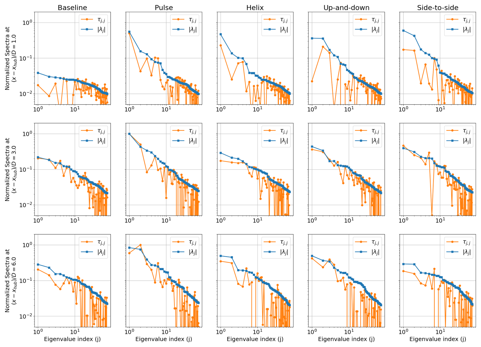
Figure 20 Energy and entrainment spectra defined by $\left|{\mathit{\lambda }}_j\right|$ and τ_j,j, respectively, for the leading 75 eigenvalues at $(x-x_{\text{hub}})/D=\mathrm{1}$, 3, and 6. The spectra are normalized on the maximum value of $\left|{\mathit{\lambda }}_j\right|$ and τ_j,j for each AWM case and streamwise location. Note that τ_j,j is not a strictly positive quantity like $\left|{\mathit{\lambda }}_j\right|$, so rapid roll-offs in the spectra occur on a log–log scale for any modes contributing to a net entrainment of mean velocity out of the wake.

The increase in the radial shear stress flux over the baseline case results in faster velocity recovery in the wake (see Figs. 21 and 22). Similar to 𝒯, the increases in mean streamwise velocity U_x are not distributed uniformly around the rotor disk; however, all AWM strategies lead to a net increase in rotor-averaged streamwise velocity over the baseline across most of the streamwise domain (see Fig. 17b). The largest increase occurs with the pulse actuation, which shows over a 4 % increase from the baseline between 2 D and 6 D downstream, while the other AWM strategies exhibit increases of 1 %–2.5 % in this region. Beyond 12 D downstream, the trend reverses, and the rotor-averaged velocity for the pulse actuation falls the furthest below the baseline value. However, at such far distances downstream, there may still be a benefit from AWM in terms of wake recovery if averaging over a larger volume. Notably, the helix forcing does sustain an increase in rotor-averaged velocity over the entire extent of the streamwise domain. In fact, by 14 D downstream, the dominant mode in terms of energy and entrainment for all AWM strategies and the baseline case is ${\mathit{\kappa }}_{\mathit{\theta }}=-\mathrm{1}$. These results suggest that strategies that excite the ${\mathit{\kappa }}_{\mathit{\theta }}=-\mathrm{1}$ mode, such as the counter-clockwise helix, may be the most effective in deep-array scenarios.

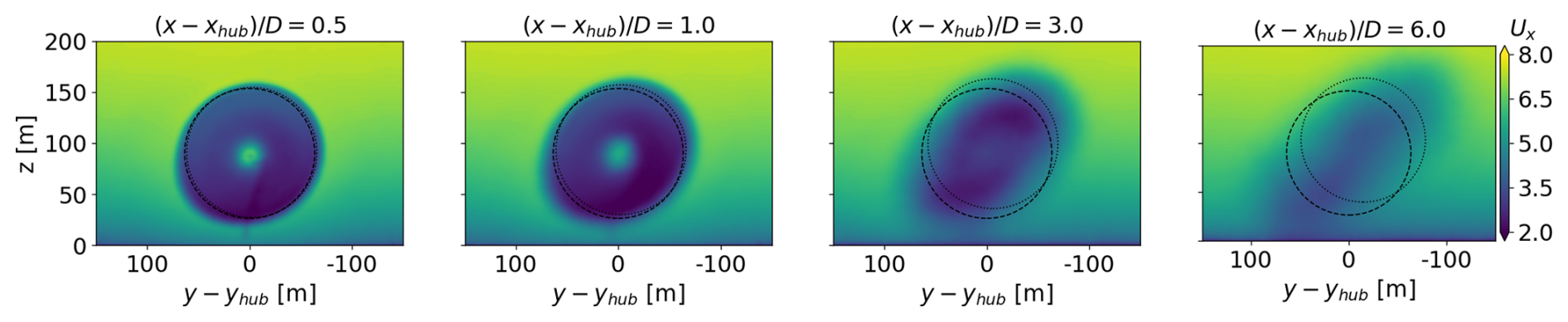
Figure 21 Contours of the streamwise velocity U_x for the baseline case at four different streamwise locations. The dashed line corresponds to the rotor disk centered at the hub height location, and the dotted line corresponds to the rotor disk centered around the wake centers.

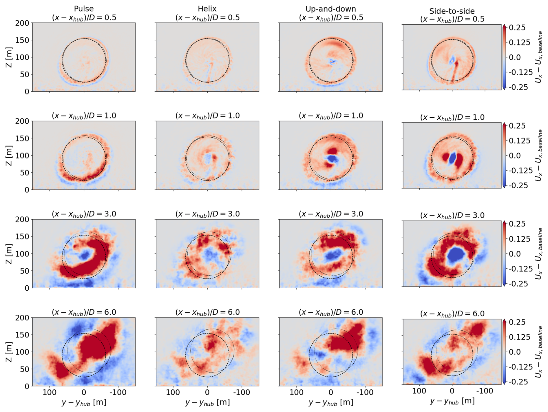
Figure 22 Contours of the baseline-subtracted streamwise velocity for each AWM case. The dashed line corresponds to the rotor disk centered at the hub height location, and the dotted line corresponds to the rotor disk centered around the wake centers.

3.3 Power and load performance metrics

Increased turbulent entrainment of mean flow enhances the performance of downstream turbines. This section demonstrates the practical benefits of improved wake recovery using a virtual two-turbine array. The gains in power typically come with the trade-off of increased loads on the upstream turbine due to pitch actuation. Therefore, the effect of different AWM strategies on turbine loads are also discussed.

The results for the second turbine are obtained through a stand-alone OpenFAST simulation of an identical NREL 2.8 MW turbine positioned downstream of the turbine simulated in the LES. AWM is applied solely to the upstream turbine, while the downstream turbine is operated using the baseline controls. Streamwise spacings ranging from 1 D to 14 D, in increments of 1 D, are analyzed for the two-turbine array for each AWM strategy considered on the upstream turbine, as well as for the baseline case, resulting in a total of 70 OpenFAST simulations. At each streamwise location, cross-flow planes are extracted from the LES and used as inflow conditions for the virtual second turbine OpenFAST simulations. This inflow data are collected from the LES over a 600 s period, the first 120 s of which are discarded as transient data when computing statistics from the outputs of OpenFAST. All statistics reported here are averaged over seven Strouhal periods. Importantly, the lateral position of the second turbine is adjusted at each streamwise location to correspond with the wake centers identified in Fig. 7c. This decision places the second turbine in the most waked environment at each streamwise location, which is where AWM is expected to be the most beneficial (Taschner et al., 2024). Recall that, in this flow, the turbine-aligned configuration does not correspond to the most waked conditions for the second turbine, primarily due to the large degree of wind veer.

The change in power from baseline operations for the virtual two-turbine array is shown in Fig. 23. It is important to note that the downstream turbine cannot follow the vertical movements of the wake, so an exact agreement with the wake analysis results presented in Sect. 3.2 is not anticipated. Nonetheless, the trends in power for the downstream turbine closely align with the rotor-averaged velocity centered with wake (compare Figs. 17b and 23). The largest increase in power for the combined two-turbine array occurs for the pulse case, with a maximum increase of 3.7 % occurring at a turbine spacing of 5 D. The pulse case performs the best for turbine spacings between 2 D and 9 D, while the other AWM strategies lead to increases of around 1 % for these spacings. These results are consistent with other studies that have examined the pulse method in highly veered ABLs (Brown et al., 2025; Frederik et al., 2025). However, for turbine spacings greater than 10 D, the pulse method underperforms baseline operations. The helix method performs the best between 10 D and 12 D, which is consistent with the sustained increase in modal energy and entrainment for the ${\mathit{\kappa }}_{\mathit{\theta }}=-\mathrm{1}$ mode observed in the far wake.

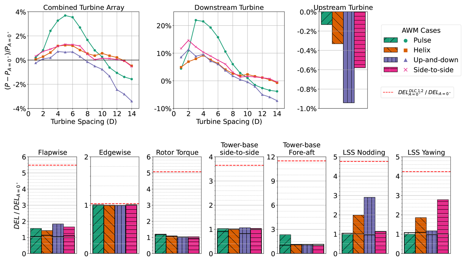
Figure 23 (Top) percent change in generated power P from the baseline case (P_A=0°) for a two-turbine array, with the turbine spacings ranging from 1 D to 14 D. The results for the upstream turbine are computed from the LES, while the downstream turbine results are obtained from a stand-alone OpenFAST simulation using YZ planes from the LES as inflow data at each streamwise location. AWM is applied to the upstream turbine with A=1.25°, while the downstream turbine is operated using baseline controls. (Bottom) baseline normalized damage equivalent loads (DELs) for seven different load channels. Solid bars indicate DELs for the upstream turbine, while the DELs for the turbine 5 D downstream are outlined in black. The dashed red line corresponds to the DELs of the turbine using baseline controls in DLC 1.2 conditions (single seed) derived from the normal turbulence model with a hub height wind speed of 6.4 m s⁻¹ (i.e. turbulence intensity of 25.90 %).

The increases in power come at the cost of increased loads on the upstream turbine. In Sect. 2.1, it was shown that the variations in the blade pitch lead to an increase in the axial force along the blade. However, the dynamic blade pitch fluctuations also affect other load channels on the turbine. In Fig. 23, loads are analyzed in terms of the baseline normalized damage equivalent loads (DELs) for seven different load channels for each AWM strategy. DELs are computed following Freebury and Musial (2000) and Ennis et al. (2018). Flapwise DELs increase between 1.4 and 1.8 times the baseline values depending on the AWM strategy. The pulse method results in a greater increase in flapwise DEL compared to the helix method at the same pitching amplitudes, which aligns with the increase in the axial force spectra observed for the pulse case compared to the helix reported in Fig. 5. Large increases in the tower base fore–aft moment are also observed for the pulse method, whereas the individual pitch control methods lead to increases in the low-speed shaft nodding and yawing moments. However, the DELs for the edgewise moment, rotor torque, and tower base side-to-side moment do not show as significant increases compared to the baseline. For a virtual turbine placed 5 D downstream, where the largest gains in combined power are found, only minor variations in the DELs are observed, likely due to increases in wake TKE, and the changes from the baseline are largely negligible across all load channels compared to the upstream turbine. In some instances, AWM even reduces the loads on downstream turbines.

To provide context for these loads, the DELs for this turbine in a Design Load Case (DLC) 1.2 environment are also included in Fig. 23. A DLC 1.2 simulation is typically used to evaluate the structural integrity and performance of the wind turbine under expected operational conditions, ensuring that it can withstand the loads and stresses it will encounter during its operational life. The DLC 1.2 results are computed here with a single seed for the turbine using baseline controls in conditions derived from the normal turbulence model with a hub height wind speed of 6.4 m s⁻¹ and a turbulence intensity of 25.90 %. This comparison is included to highlight the fact that AWM is particularly well suited to stable ABL conditions with low TI, where the significant increases in DELs over the baseline largely remain much smaller than the loads on the turbine in typical design environments.

4 Conclusions

In this work, a SPOD analysis was developed to track the coherent flow structures induced by AWM throughout the streamwise domain, including their origins in the turbine induction field, growth in the near-wake region, and subsequent evolution and energy transfers in the far wake. SPOD is shown to be a particularly useful tool in the context of AWM because it decouples structures in the flow, allowing the wavenumber and frequency inputs to the turbine controller to be translated directly to the wake. The modes directly forced by the blade pitch fluctuations are found to be the dominant flow structures in the near-wake region, which originate around 0.5 D ahead of the turbine. However, as the wake evolves downstream, modal interactions excite other flow structures within the wake, which often exceed the energy of the near-wake structures. Further, it is demonstrated that a complete description of AWM effects requires considering correlations between all three velocity components, as significant radial and azimuthal modifications to the wake are induced, in addition to the those in the streamwise direction.

The SPOD analysis was also connected to conventional wake mixing quantities of interests for different AWM strategies. A new modal decomposition of the radial shear stress flux was developed to measure the contribution of each flow structure in the wake to mean flow turbulent entrainment. This established a quantitative connection between the kinetic energy of coherent structures in the wake and their contribution to turbulent entrainment. The leading flow structures in terms of TKE are found to be primarily responsible for velocity recovery mechanisms in the wake; however, the relationship between modal energy and entrainment is not necessarily directly proportional. In terms of blade loading, a correlation between the spectrum of the axial force along the blade and the spectral characteristics of the induction field was established through the SPOD eigenvalues. Additionally, the modal structure of the induction field suggested that the individual pitch control strategies divert flow around regions of higher blockage, leading to a decrease in the axial blade force compared to collective pitch actuation. A complete end-to-end description of the actuated flow is thus provided. For example, the pulse method (1) induces an axisymmetric modification to the induction field, which (2) results in the largest increase in axial loading amongst AWM strategies; this increase in thrust (3) generates the most dominant coherent structure and largest enhancement of modal energy in the near wake, which (4) leads to greater turbulent entrainment and faster velocity recovery downstream for all AWM strategies; lastly, this (5) ultimately results in the largest increase in generator power for the downstream turbine.

A key observation is that, for the cases considered in this study, the effectiveness of AWM relied on exciting the inherent flow structures in the turbulence of the baseline wake. SPOD, therefore, proved equally useful for analyzing the structure of the wake under baseline operations as it did for the AWM control strategies. For example, the performance of the pulse method was primarily attributed to turbulent entrainment from the κ_θ=1 and 2 modes. These modes were found to be the dominant flow structures in the near-wake region of the baseline case, suggesting that the effectiveness of the pulse method was due to its ability to enhance the dominant structures in the non-actuated wake. It is important to note that this does not imply that the pulse method will perform optimally under all ABL conditions but rather that the effects of ABL characteristics on the modal structure of the baseline wake must be considered when designing a control strategy. A broader range of atmospheric conditions should be examined, including variations in shear, veer, swirl, stratification, TI, and wind speeds to strengthen the relationship between AWM performance and the coherent structures in the baseline wake. Such insights may enable the optimal design of wind farm flow control with respect to power and load trade-offs, such as maintaining power benefits with lower pitching amplitudes by targeting the optimal wake structures.

Similarly, the findings of this study highlight the importance of understanding the non-linear mechanism responsible for transferring energy between coherent structures in the wake. While SPOD is used here to track modal TKE and entrainment, it does not provide an explanation for how energy is transferred between SPOD modes. For example, why does the pulse method excite the κ_θ=1 and 2 wavenumbers in the flow, even though only the κ_θ=0 wavenumber is directly forced by the controller? Addressing such questions will be crucial for future work in optimizing AWM strategies, which may rely on understanding triadic interactions between the forced AWM mode and the other turbulent scales.

Lastly, recent work suggests that a linear stability-based reduced-order model may be effective for representing the effects of AWM-induced coherent structures on the mean flow (Cheung et al., 2025). The SPOD results presented here will be useful for such model developments, as it will help to characterize the growth rates of coherent structures in the wake, which are inputs to the linear stability analysis. Similarly, projection-based reduced-order models including resolvent or DMD-based models (Muscari et al., 2022; Gutknecht et al., 2023) would also benefit from the SPOD formulation used in this study. For either approach, the eigenvalue spectra reported here indicate that it may not be sufficient to only model the forced coherent structures in the wake, but that modeling interactions with other large-scale structures in the wake is necessary for accurately representing AWM dynamics.

Appendix A: SPOD analysis of the individual velocity components

The SPOD formulation in Sect. 2.2 includes correlations between all three cylindrical velocity field components $\mathit{u}=(u_x,u_r,u_{\mathit{\theta }})$ in the definition of the cross-spectral density tensor $\mathbf{S}(r,r^{\prime })=\langle \widehat{\mathit{u}}(r,{\mathit{\kappa }}_{\mathit{\theta }},\mathit{\omega }){\widehat{\mathit{u}}}^{*}(r^{\prime },{\mathit{\kappa }}_{\mathit{\theta }},\mathit{\omega })\rangle$. Here, the SPOD analysis is repeated for each diagonal element of S, namely $S_{\mathrm{11}}(r,r^{\prime })=\langle {\widehat{u}}_x(r,{\mathit{\kappa }}_{\mathit{\theta }},\mathit{\omega }){\widehat{u}}_x^{*}(r^{\prime },{\mathit{\kappa }}_{\mathit{\theta }},\mathit{\omega })\rangle$, $S_{\mathrm{22}}(r,r^{\prime })=\langle {\widehat{u}}_r(r,{\mathit{\kappa }}_{\mathit{\theta }},\mathit{\omega }){\widehat{u}}_r^{*}(r^{\prime },{\mathit{\kappa }}_{\mathit{\theta }},\mathit{\omega })\rangle$, and $S_{\mathrm{33}}(r,r^{\prime })=\langle {\widehat{u}}_{\mathit{\theta }}(r,{\mathit{\kappa }}_{\mathit{\theta }},\mathit{\omega }){\widehat{u}}_{\mathit{\theta }}^{*}(r^{\prime },{\mathit{\kappa }}_{\mathit{\theta }},\mathit{\omega })\rangle$.

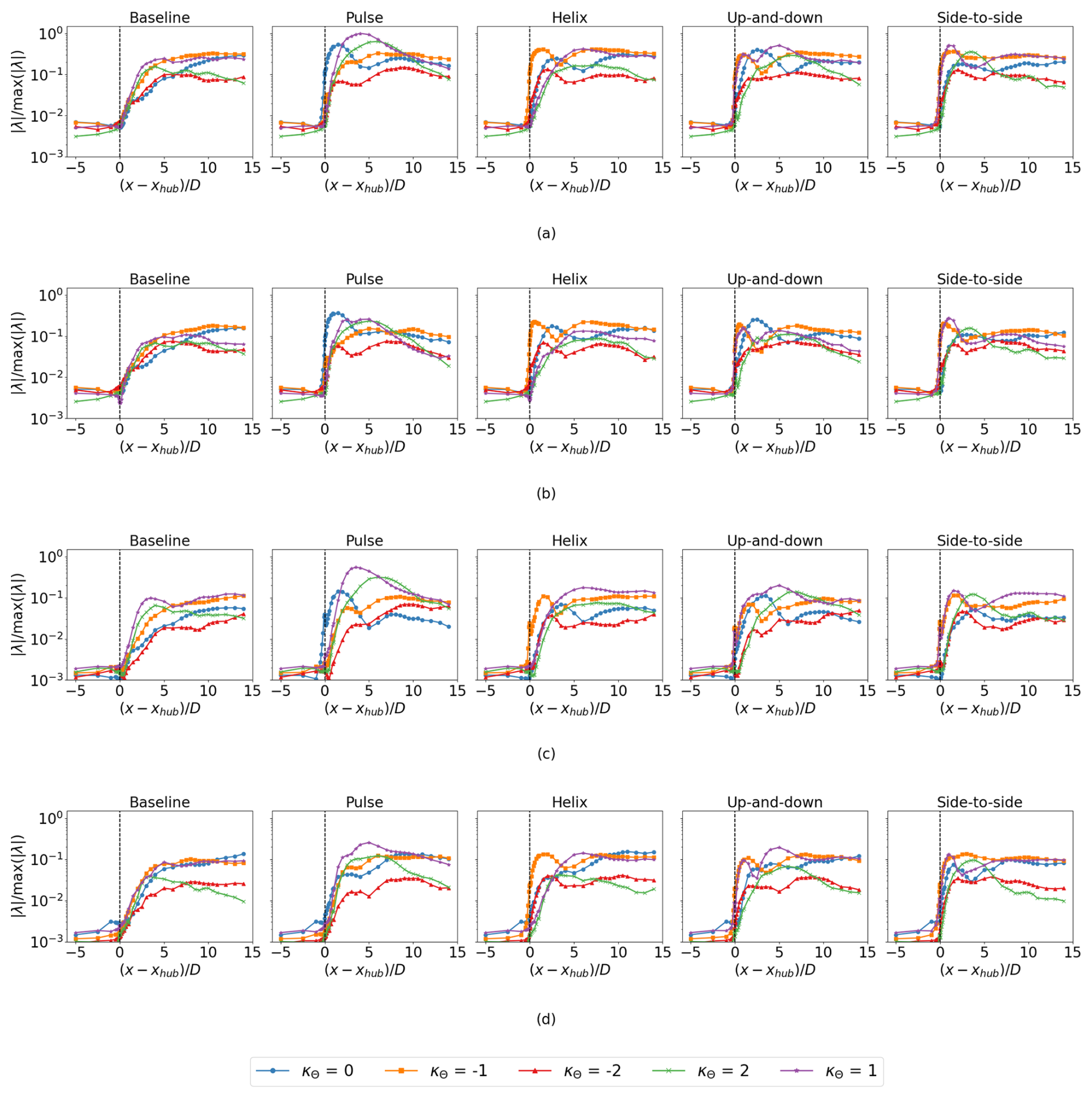
Figure A1 Eigenvalues of (a) S, (b) S₁₁, (c) S₂₂, and (d) S₃₃ corresponding to velocity correlations in u, u_x, u_r, and u_θ, respectively. Eigenvalues at St=0.3 are shown for κ_θ=0, ±1, and ±2.

The eigenvalues of the cross-spectral density tensor S and its diagonal components at St=0.3 are shown in Fig. A1 across the streamwise extent of the domain. AWM generally induces a consistent modal response in the streamwise, radial, and azimuthal velocity components throughout the evolution of the wake, although there are differences in kinetic energy between velocity components. In the near-wake region, the dominant flow structure occurs at the forced azimuthal wavenumber in all three velocity components, i.e. κ_θ=0, ${\mathit{\kappa }}_{\mathit{\theta }}=-\mathrm{1}$, and ${\mathit{\kappa }}_{\mathit{\theta }}=\pm \mathrm{1}$ for the pulse, helix, and mixed-mode actuations, respectively. The most energetic structures in this region are found in the streamwise velocity component, which is expected since the azimuthal and temporal variations in the blade pitch are designed to induce a significant axial force along the blade. However, by 4 D to 5 D downstream, the energetic structures (Fig. A1) and wake TKE as a whole (Fig. 14) are primarily driven by the in-plane velocities. For instance, the largest eigenvalue for S across all streamwise locations and AWM strategies occurs 4 D downstream for the pulse case at κ_θ=1, which is driven by the radial velocity component, as is the subsequent increase in κ_θ=2 mode for this case. These two modes are also the dominant structures in u_r for the baseline wake and were shown to contribute significantly to mean flow turbulent entrainment (see Sect. 3.2). This suggests that the effectiveness of the pulse strategy is a result of axisymmetric streamwise forcing exciting higher-order radial velocity flow structures in the non-actuated wake. Similarly, at 6 D downstream, κ_θ=1 is the dominant mode for all of the non-axisymmetric forcing strategies, which are driven by the radial and azimuthal velocity components. In the far wake, the modal TKE generally returns to the baseline values for all AWM strategies and velocity components.

Appendix B: discrete SPOD solution

The computational formulation in Sect. 2.2 results in a discrete complex velocity Fourier matrix $\widehat{\mathbf{U}}\in {\mathbb{C}}^{N_{\mathrm{R}}\times N_{\mathrm{B}}}$ for each azimuthal wavenumber κ_θ and frequency ω at each streamwise location (see Towne et al., 2018, for additional details on the formulation of $\widehat{\mathbf{U}}$). Here, N_R is the number of discrete points in the radial domain, and N_B is the number of blocks of data resulting from the windowed Fourier transform in time. The analytical eigenvalue problem in Eq. (3) can then be represented discretely as

$$\begin{array}{}\text{(B1)}& {\displaystyle }{\displaystyle }\mathbf{SW}\mathit{\psi }=\mathit{\lambda }\mathit{\psi },\end{array}$$

where ψ and λ are a discrete eigenvector and eigenvalue pair and $\mathbf{W}\in {\mathbb{R}}^{N_{\mathrm{R}}\times N_{\mathrm{R}}}$ is a positive definite Hermitian weighting matrix that accounts for the numerical quadrature of the radial integral. Here, the matrix W is defined through a one-third Simpson's rule. The matrix $\mathbf{S}\sim \frac{\mathrm{1}}{N_{\mathrm{B}}}\widehat{\mathbf{U}}{\widehat{\mathbf{U}}}^H\in {\mathbb{C}}^{N_{\mathrm{R}}\times N_{\mathrm{R}}}$ is a discrete representation of the cross-spectral density tensor, approximated from an ensemble average of velocity correlations over N_B flow realizations. A difficulty in solving Eq. (B1) is that the matrix product SW is not generally Hermitian. However, a Hermitian problem is achieved by multiplying B1 by ${\mathbf{W}}^{\mathrm{1}/\mathrm{2}}$:

$$\begin{array}{}\text{(B2)}& {\displaystyle }{\displaystyle }\stackrel{\mathrm{̃}}{\mathbf{S}}\stackrel{\mathrm{̃}}{\mathit{\psi }}=\mathit{\lambda }\stackrel{\mathrm{̃}}{\mathit{\psi }},\end{array}$$

where $\stackrel{\mathrm{̃}}{\mathbf{S}}={\mathbf{W}}^{\mathrm{1}/\mathrm{2}}{\mathbf{SW}}^{\mathrm{1}/\mathrm{2}}$ and $\stackrel{\mathrm{̃}}{\mathit{\psi }}$. For cases where N_B<N_R, there are at most N_B non-zero eigenvalues of S. Therefore, Eq. (B2) can be solved efficiently by performing a low-rank SVD of $\frac{\mathrm{1}}{\sqrt{N_{\mathrm{B}}}}{\mathbf{W}}^{\mathrm{1}/\mathrm{2}}\widehat{\mathbf{U}}=\mathbf{L}\mathbf{\Sigma }{\mathbf{R}}^H$, where L and R are the left and right singular vectors and Σ is the matrix of singular values. Using this decomposition, $\stackrel{\mathrm{̃}}{\mathbf{S}}$ can be expressed as $\stackrel{\mathrm{̃}}{\mathbf{S}}=\left(\mathbf{L}\mathbf{\Sigma }{\mathbf{R}}^H\right)\left(\mathbf{R}\mathbf{\Sigma }{\mathbf{L}}^H\right)=\mathbf{L}{\mathbf{\Sigma }}^{\mathrm{2}}\mathbf{L}$. Thus, the eigenvalues λ are given by the square of the singular values, and the eigenvectors $\stackrel{\mathrm{̃}}{\mathit{\psi }}$ are given by the left singular vectors. Finally, the eigenvectors of the original eigenvalue problem (Eq. B1) are obtained by multiplying L by ${\mathbf{W}}^{-\mathrm{1}/\mathrm{2}}$, i.e. $\mathit{\psi }={\mathbf{W}}^{-\mathrm{1}/\mathrm{2}}\stackrel{\mathrm{̃}}{\mathit{\psi }}={\mathbf{W}}^{-\mathrm{1}/\mathrm{2}}\mathbf{L}$.