Simulating run-to-failure SCADA time series to enhance wind turbine fault detection and prognosis

Wind turbine supervisory control and data acquisition (SCADA) datasets available for research usually contain a limited number of failure events. This limitation hinders the successful application of deep learning (DL) methods for fault detection and prognosis, as they require large datasets for robust training and generalisation. This work proposes a method using conditional generative adversarial networks (cGANs) to generate synthetic SCADA time series that replicate wind turbine behaviour under controllable operational, environmental, and degradation conditions. Given a set of SCADA time series representing these conditions, the cGAN generates temperature and pressure time series simulating gearbox operation. Results show that augmenting the training set of an artificial neural network (ANN) fault detection model with synthetic time series reduces false positives in the detected gearbox faults by 84 % on average, enabling the model to blindly detect a fault in a test wind turbine without prior knowledge of the event. Furthermore, training a convolutional autoencoder-based unsupervised health indicator (HI) model with both real and synthetic SCADA time series leads to an HI that more accurately captures the expected degradation trend. Using this HI, the gearbox's remaining useful life (RUL) can be predicted within the defined error bounds from around 4.5 months before the detection of the fault, while the HI obtained without the synthetic data fails to produce reliable RUL estimations.

1 Introduction

State-of-the-art deep learning (DL) methods for wind turbine fault detection and prognosis rely on large datasets for robust training and generalisation. However, component failures in wind turbines are rare events (Spinato et al., 2009), and wind farm operators are often reluctant to disclose detailed information about them due to privacy concerns (Chatterjee and Dethlefs, 2021). Therefore, supervisory control and data acquisition (SCADA) datasets available for research usually include very few failure events, limiting the successful implementation of DL methods. A viable solution to this challenge is to simulate new failure events within SCADA datasets. This involves generating time series data that mimic sensor signals reflecting turbine component behaviour as degradation progresses over a specific time window leading to failure. Rather than merely replicating existing failure event signals, these synthetically generated run-to-failure time series should instead capture diverse degradation scenarios under varying operational and environmental conditions. This diversity is crucial for enhancing the training data of DL fault detection and prognosis models, improving their robustness and practicality.

Existing approaches for generating synthetic signals have mostly used physics-based and hybrid physics-data-driven models of wind turbines. They often simulate damage by methods such as inserting additional mass or reducing local structural stiffness. For example, synthetic vibrational signals generated using the OpenFAST software (Jonkman et al., 2022) have been used to validate condition monitoring methods in Tatsis et al. (2017), Tatsis et al. (2021), and Song et al. (2024). However, they are unsuitable for training DL methods to be applied to real wind turbines with different configurations. In Pujana et al. (2023), a hybrid digital twin of a wind turbine drivetrain is developed to generate synthetic stator winding temperature signals, with the temperature increase due to a generator failure modelled as a heat exchanger. These synthetic signals are used to train a fault detection model. While useful, these methods oversimplify the actual component behaviour and cannot model gradual degradation. Therefore, they fail to generate realistic run-to-failure sequences across multiple SCADA signals, which are critical for prognostic applications.

Data-driven approaches for generating synthetic SCADA time series are rare in the literature. An artificial neural network (ANN)-based framework for generating synthetic SCADA signals, given operational, environmental, and degradation conditions, is proposed in Eftekhari Milani et al. (2024a). While the generated synthetic signals are in good agreement with the corresponding field data, this approach assumes that sensor signals at each timestamp are deterministic functions of the current conditions. This assumption overlooks the inertia and temporal dependencies present in SCADA signals. These signals, especially temperature data, often exhibit significant inertia, with measurements strongly dependent on their previous values (Mello et al., 2021). Furthermore, this approach does not address the inherent stochasticity of SCADA signals and does not demonstrate whether it can simulate new failure events.

Generative adversarial networks (GANs) (Goodfellow et al., 2020) have been proven successful in generating diverse and realistic synthetic data across many domains, including images (Shorten and Khoshgoftaar, 2019), text (Li et al., 2018), audio (Liu et al., 2022), and video (Chu et al., 2020). These models consist of two neural networks trained in a competitive framework: a generator generating realistic-looking synthetic samples and a discriminator evaluating whether the data are real or synthetic. In the wind turbine SCADA data domain, the application of GANs has been mostly limited to addressing class imbalances in fault detection tasks by augmenting faulty data instances. For example, faulty data instances are generated in Liu et al. (2019) to enhance fault detection performance. In Wang et al. (2022), a variant of GAN called the least squares GAN is used to generate synthetic data instances and improve the performance of an autoencoder-based condition monitoring framework. Similarly, in Liu et al. (2023), a GAN is used to overcome the limitation of scarce faulty data by generating synthetic faulty instances, which are then used to enhance the performance of an autoencoder-based anomaly detection method. These methods outperform more traditional oversampling approaches (Antoniou et al., 2017), such as those based on the synthetic minority oversampling technique (SMOTE) (Chawla et al., 2002), which have been extensively used to address the problem of class imbalance in SCADA datasets (Peng et al., 2020; Yang et al., 2021; Li et al., 2023; Tao et al., 2024). However, they are limited to generating individual signal instances rather than run-to-failure time series. Another limitation of these methods is that they cannot simulate entirely new failure events and are limited to oversampling faulty data instances corresponding to existing failure events in SCADA datasets (Chesterman et al., 2023). Extending these approaches to generate entire time series is challenging, as a generative model must learn not only the feature distributions but also their temporal dynamics. Furthermore, it must generate a diverse set of time series under predefined operational, environmental, and degradation conditions to be useful for wind turbine fault detection and prognosis.

This work addresses these limitations by developing a method based on a conditional GAN (cGAN) (Mirza and Osindero, 2014). Unlike the standard vanilla GAN, the proposed model allows conditioning each generated signal instance to a vector of predefined conditions, including component degradation levels and SCADA measurements related to environmental conditions and the operational states of the wind turbine. To capture temporal dynamics of the signal instances, gated recurrent unit (GRU)-based recurrent neural networks (Cho et al., 2014) are used for both the generator and the discriminator networks, enabling the model to retain a memory of condition vectors from previous timestamps. Furthermore, as suggested by Yoon et al. (2019), a supervised loss term is added to the generator's training loss function to enhance the cGAN's ability to generate realistic SCADA time series. The effectiveness of this approach for fault detection and remaining useful life (RUL) prediction is demonstrated using field SCADA data. The results show that augmenting field data with synthetic time series generated by the cGAN significantly reduces false positives caused by the scarcity of failure events in training data. This enables the model to blindly detect a fault in one of the test wind turbines without prior knowledge of the event. Furthermore, including synthetic time series enhances the performance of a health indicator (HI) construction model. The resulting HIs better capture the degradation trend than those generated without the synthetic data, leading to more accurate RUL predictions. The rest of this paper is organised as follows. Section 2 describes the method developed for synthetic SCADA time series generation. Section 3 introduces the SCADA dataset used, data preprocessing, selected signals, and the healthy and faulty wind turbines. Sections 4 and 5 present the application of the proposed method in fault detection and RUL prediction, respectively. Finally, conclusions are drawn, and future work is discussed in Sect. 6.

2 Generation of synthetic SCADA signals

A set of SCADA signals representing the operation of a wind turbine component, such as gearbox temperature and pressure signals, is a discrete multivariate time series $\mathbf{S}=\mathit{\left\{}{s}_{i,t}\mathit{\right\}}$ with distribution p_s, where $t=\mathrm{1},\mathrm{\dots },T$, $i=\mathrm{1},\mathrm{\dots },N_{\mathrm{s}}$, N_s is the number of component signals, t is the time instance, and T is the length of the dataset. Similarly, $\mathbf{O}=\mathit{\left\{}{o}_{i,t}\mathit{\right\}}$, where $i=\mathrm{1},\mathrm{\dots },N_{\mathrm{o}}$, and $\mathbf{E}=\mathit{\left\{}{e}_{i,t}\mathit{\right\}}$, where $i=\mathrm{1},\mathrm{\dots },N_{\mathrm{e}}$, are sets of SCADA signals representing operational and environmental conditions over the same time interval $t=\mathrm{1},\mathrm{\dots },T$, such as rotor speed and ambient temperature, with N_o and N_e being the number of signals representing these conditions, respectively. D is an HI representing the degradation of the component at each point in time, which can be extracted from the SCADA signals. The set of $\mathit{\{}\mathbf{O},\mathbf{E},D\mathit{\}}$ is called the condition time series $\mathbf{C}=\mathit{\left\{}{c}_{i,t}\mathit{\right\}}$, where $i=\mathrm{1},\mathrm{\dots },N_c$, and $N_c=N_{\mathrm{o}}+N_{\mathrm{e}}+\mathrm{1}$ is the number of condition signals.

It is assumed that S is a function of C (Eftekhari Milani et al., 2024a), with some stochasticity inherent in the SCADA signals. At each instance t, s_t is a function of not only c_t but also all the previous instances due to the inertia inherent in the SCADA signals. However, in practice, this dependence becomes negligible beyond a certain time window. This relationship can be expressed through a stochastic generative function ℱ:

$$\begin{array}{}\text{(1)}& {\mathit{s}}_t=\mathcal{F}({\mathit{c}}_{\mathrm{1}:t},{\mathit{z}}_t),\end{array}$$

where z_t is a vector of random noise with distribution p_z. The objective of this work is to model ℱ through a GAN-based framework and use it to generate a set of synthetic SCADA signals S^s given any C.

2.1 HI construction

As mentioned in the previous section, D is an HI extracted from the SCADA dataset and, together with O and E, forms the condition time series C. In this work, D is obtained using the unsupervised method developed in Eftekhari Milani et al. (2024b), where it is demonstrated that it can construct HIs that track the true component degradation trend more accurately than other methods proposed in the literature. This approach adopts a convolutional autoencoder (CAE), which is trained using a hybrid of particle swarm optimisation (PSO) and backpropagation to simultaneously maximise the HI monotonicity built in the middle layer and minimise the reconstruction error. Due to the generally irreversible nature of component degradation, an HI is expected to demonstrate a monotonic trend, and monotonicity has been widely used as one of the main criteria to build HIs (She and Jia, 2019; Yang et al., 2022). Therefore, maximising monotonicity leads to an HI that better represents the component degradation, leading to a more accurate RUL prediction. The training fitness function to be maximised is

$$\begin{array}{}\text{(2)}& f=f_{\mathrm{M}}-f_{\mathrm{R}}-f_{\mathrm{0}}-f_{\mathrm{1}},\end{array}$$

where f_M is the monotonicity of the HI built in the middle layer of the CAE, measured using the Mann–Kendall (MK) metric (Pohlert, 2015); f_R is the CAE reconstruction loss, i.e., the mean squared error (MSE) of the difference between the CAE input and output; $f_{\mathrm{0}}=\left|\mathrm{HI}\right(\mathrm{0}\left)\right|$ is the absolute HI value at its initial timestamp; and $f_{\mathrm{1}}=|\mathrm{1}-\mathrm{HI}(\mathrm{end}\left)\right|$, where HI(end) is the HI value at its final timestamp. Maximising f corresponds to minimising both f₀ and f₁ and training the CAE to associate the healthy state at the initial timestamp with an HI value of 0 and the failed state at the final timestamp with an HI value of 1. In this work, f₀ is removed from f because the component is not necessarily in a pristine state at the initial timestamp of a run-to-failure SCADA time series.

SCADA measurements are characterised by high noise levels and varying operational and environmental conditions. These factors make it more challenging for the CAE to effectively reconstruct and denoise the signals compared to more controlled vibration signals obtained from bearing test beds used in Eftekhari Milani et al. (2024b). Therefore, in this work, an additional term f_SD is considered, which measures the average weekly rolling standard deviation of the HI, and minimising this term leads to a less noisy HI. An equal weight of 1 for the four terms f_M, f_R, f₁, and f_SD results in slow convergence during the training process due to the slow minimisation of the reconstruction error, and the obtained training HI tends to be noisy. For this reason, the weights of the f_R and f_SD terms are set to 3 using trial and error to balance the four terms and resolve these issues.

The CAE training fitness function thus used in this work is

$$\begin{array}{}\text{(3)}& f=f_{\mathrm{M}}-\mathrm{3}{f}_{\mathrm{R}}-f_{\mathrm{1}}-\mathrm{3}{f}_{\mathrm{SD}}.\end{array}$$

The CAE architecture and the training algorithm hyperparameters are set according to those proposed in Eftekhari Milani et al. (2024b).

Since wind turbines operate under highly variable operational and environmental conditions, the constructed HIs usually exhibit local variations, which can reduce the RUL prediction accuracy. To mitigate these variations, a post-processing algorithm is developed, leveraging the usual irreversible nature of component degradation. As shown in Algorithm 1, a curve is fitted to the HI using the non-parametric locally weighted scatterplot smoothing (LOWESS) regression approach (Cleveland and Devlin, 1988). This curve is then subtracted from the HI, and subsequently, the cumulative maximum of the curve is re-added to the HI.

Algorithm 1 HI post-processing algorithm.

1. Fit a curve to the HI using LOESS.

2. Compute residue:  $residue=HI-curve$.

3. Compute curve_cm:  $curv{e}_{cm}\left(t\right)=max\left[curve\right(\mathrm{1}:t\left)\right]$.

4. Compute the post-processed HI:  $H{I}_{pp}=residue+curv{e}_{cm}$.

Figure 1 provides a visual explanation of this algorithm and its impact on RUL prediction. Figure 1a shows a hypothetical HI and a curve fitted using LOWESS. In Fig. 1b and c, which show the HI at t=200 s and t=300 s, respectively, it is evident that the slope of the regression line oscillates between negative and positive values. This undesirable behaviour is resolved after post-processing the HI with Algorithm 1, as shown in Fig. 1d–f.

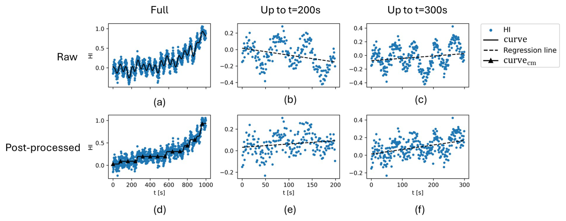
Figure 1 Example of HI post-processing on a hypothetical HI: (a–c) raw HI, its first 200 s, and its first 300 s and (d–f) post-processed HI, its first 200 s, and its first 300 s.

2.2 Vanilla GAN

GANs consist of two neural networks: a generator (𝒢), which takes an input vector of unit Gaussian random noise and generates a synthetic sample, and a discriminator (𝒟), which, given any sample, outputs the probability of it being real (not synthesised). These neural networks are trained in an adversarial framework where the generator is trained to generate increasingly realistic-looking synthetic samples to deceive the discriminator and the discriminator is trained to detect these synthetic samples with higher accuracy (Goodfellow et al., 2020). In the context of SCADA signals, the generator receives a noise vector z_t as input and is trained to generate synthetic signals ${\mathit{s}}_t^s$ that match the distribution of the real signals s_t used to train the GAN. The discriminator is trained to output a probability of 1 when the data are real and 0 when they are synthetic, minimising the loss function:

$$\begin{array}{}\text{(4)}& {\mathcal{L}}_{\mathcal{D}}^v=-{\mathbb{E}}_{{\mathit{s}}_t\sim p_s}\left[\log \mathcal{D}\left({\mathit{s}}_t\right)\right]-{\mathbb{E}}_{{\mathit{z}}_t\sim p_z}\left[\log \left(\mathrm{1}-\mathcal{D}\left(\mathcal{G}\left({\mathit{z}}_t\right)\right)\right)\right],\end{array}$$

where 𝔼 denotes the expected value. The generator is trained to deceive the discriminator by generating synthetic samples that it classifies as real, assigning a label of 1. It minimises the loss function:

$$\begin{array}{}\text{(5)}& {\mathcal{L}}_{\mathcal{G}}^v=-{\mathbb{E}}_{{\mathit{z}}_t\sim p_z}\left[\log \mathcal{D}\left(\mathcal{G}\left({\mathit{z}}_t\right)\right)\right].\end{array}$$

The overall objective is a min–max game between the generator and the discriminator:

$$\begin{array}{}\text{(6)}& \begin{array}{rl}\underset{\mathcal{G}}{min}\underset{\mathcal{D}}{max}V\left(\mathcal{D},\mathcal{G}\right)& ={\mathbb{E}}_{{\mathit{s}}_t\sim p_s}\left[\log \mathcal{D}\left({\mathit{s}}_t\right)\right]\\ & +{\mathbb{E}}_{{\mathit{z}}_t\sim p_z}\left[\log \left(\mathrm{1}-\mathcal{D}\left(\mathcal{G}\left({\mathit{z}}_t\right)\right)\right)\right],\end{array}\end{array}$$

where the discriminator tries to maximise the value function V, and the generator tries to minimise it.

2.3 Proposed method for generating synthetic SCADA signals

A vanilla GAN treats S as a group of independent samples s_t and models only the signal distribution p(s_t), neglecting the temporal dependencies (Yoon et al., 2019). Furthermore, signals are generated based only on a random noise vector. Therefore, the objective of this work is to develop a GAN-based framework that effectively models ℱ in Eq. (1):

1. by conditioning the signal generation on both the condition vector C and a random noise vector and

2. by modelling the temporal dynamics of SCADA signals by conditioning the signal generation at each timestamp on information from previous timestamps, in addition to the current one.

In other words, rather than modelling the marginal distribution of the signals p(s_t), the framework should model the conditional distribution $p\left({\mathit{s}}_t\right|{\mathit{c}}_{\mathrm{1}:t})$.

The first task above is achieved by adopting a cGAN framework (Mirza and Osindero, 2014), which allows the input of a condition vector at each timestamp t to the generator and the discriminator, based on which the samples are generated. The loss functions of the discriminator and generator then become

$$\begin{array}{}\text{(7)}& {\displaystyle }\begin{array}{rl}{\mathcal{L}}_{\mathcal{D}}& =-{\mathbb{E}}_{{\mathit{s}}_t\sim p_{\mathrm{s}}}\left[\log \mathcal{D}\left({\mathit{s}}_t|{\mathit{c}}_t\right)\right]\\ & -{\mathbb{E}}_{{\mathit{z}}_t\sim p_z}\left[\log \left(\mathrm{1}-\mathcal{D}\left(\mathcal{G}\left({\mathit{z}}_t|{\mathit{c}}_t\right)\right)\right)\right],\end{array}\text{(8)}& {\displaystyle }{\mathcal{L}}_{\mathcal{G}}=-{\mathbb{E}}_{{\mathit{z}}_t\sim p_z}\left[\log \mathcal{D}\left(\mathcal{G}\left({\mathit{z}}_t|{\mathit{c}}_t\right)\right)\right].\end{array}$$

The second task is achieved by using a recurrent neural network (RNN) for both the generator and the discriminator, allowing them to retain information from previous timestamps at each t. Additionally, as suggested in Yoon et al. (2019), a supervised loss term ℒ_S is incorporated into the GAN generator loss function to further enhance temporal consistency.

$$\begin{array}{}\text{(9)}& {\mathcal{L}}_{\mathrm{S}}={\mathbb{E}}_{\begin{array}{c}{\mathit{s}}_t\sim p_{\mathrm{s}}\\ {\mathit{z}}_{\mathrm{t}}\sim p_z\end{array}}\left[\left|\right|{\mathit{s}}_t-\mathcal{G}\left({\mathit{z}}_t|{\mathit{c}}_t\right)|{|}_{\mathrm{2}}^{\mathrm{2}}\right]\end{array}$$

This loss term minimises the Euclidean distance between the true and generated signals during the training phase. The modified generator loss function then becomes

$$\begin{array}{}\text{(10)}& \mathcal{L}{{}^{\prime }}_{\mathcal{G}}={\mathcal{L}}_{\mathcal{G}}+{\mathcal{L}}_{\mathrm{S}}.\end{array}$$

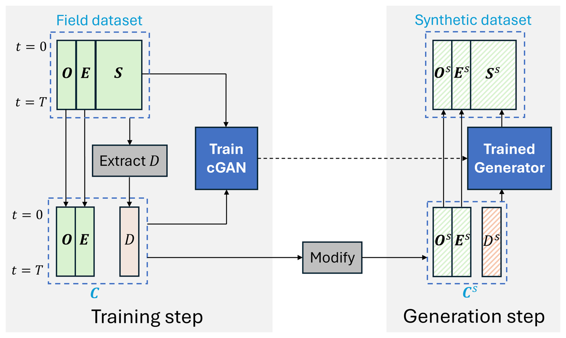
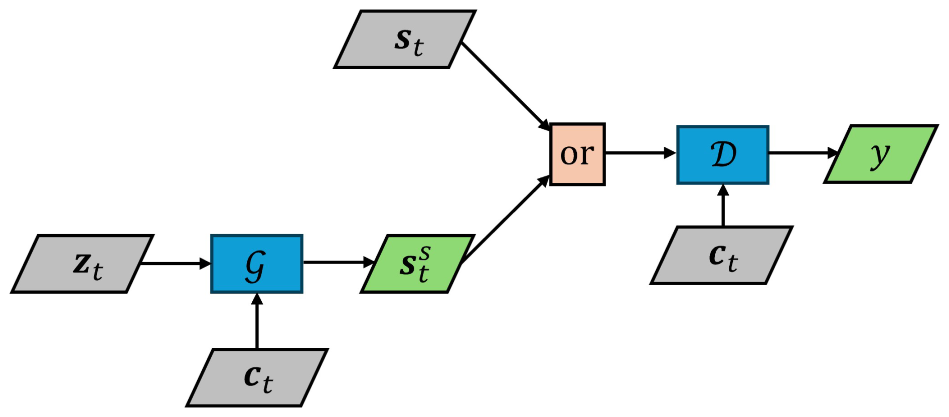
The flowchart of the cGAN-based synthetic SCADA signal generation framework is shown in Fig. 2. In this work, gated recurrent unit (GRU)-based RNNs have been used, as GRU cells achieve performance comparable to Long Short-Term Memory (LSTM) cells while having fewer parameters. This makes them more efficient, faster to train, and less prone to overfitting (Chung et al., 2014). The flowchart of the cGAN model is shown in Fig. 3, where $y=p(\mathit{x}={\mathit{s}}_t|{\mathit{c}}_t)$, with x being the input to the discriminator.

Figure 2 Flowchart of the cGAN-based synthetic SCADA signal generation framework.

Figure 3 Flowchart of the cGAN model.

The architectures of the generator and the discriminator are shown in Fig. 4:

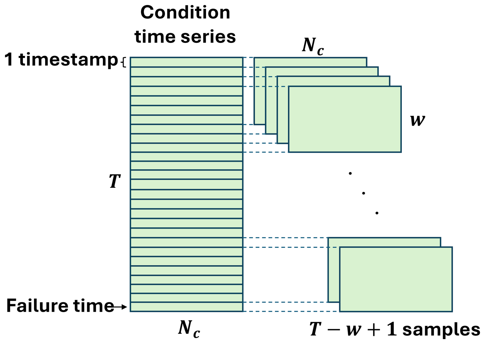
1. w is the length of a rolling time window applied to C before being fed into the GRU layer in both networks. This transforms the shape of C from (T,N_c) to $(T-w+\mathrm{1},w,N_c)$ and is shown in Fig. 5. The window length w introduces a trade-off between model complexity and performance. A larger window allows more information to be captured at each time frame from earlier signal values, at the expense of increased computational burden. In this study, this parameter is set to 10, since the HI obtained from the training wind turbine remained mostly unchanged for larger window length values.

2. Λ denotes the leaky ReLU activation function defined below with α=0.2.

$$\begin{array}{}\text{(11)}& \mathrm{\Lambda }\left(x\right)=\left\{\begin{array}{ll}x& \text{if }x\ge \mathrm{0}\\ \mathit{\alpha }x& \text{if }x<\mathrm{0}\end{array}\right.\end{array}$$

Figure 4 Architecture of the generator (left) and the discriminator (right).

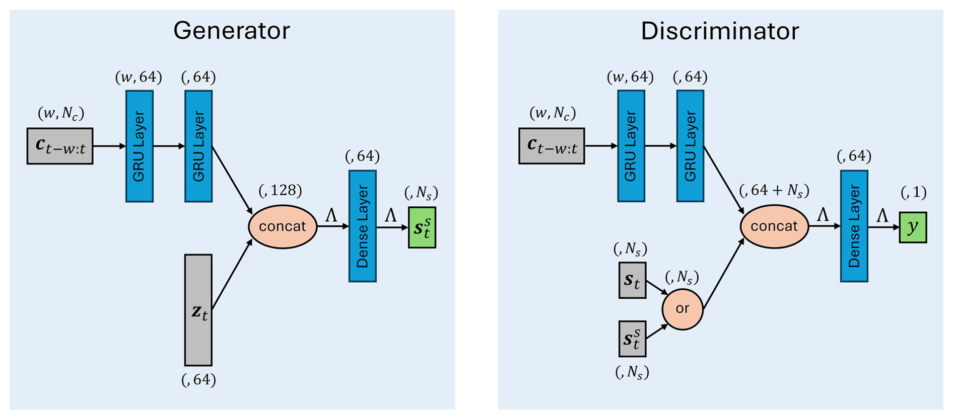
In both the generator and the discriminator, the condition signals C pass through two recurrent layers with 64 GRU cells. The output vector is concatenated with the random vector in the generator and with the real or synthetic component signals, S or S^s, in the discriminator. The result is then input to a dense layer with 64 neurons, followed by the output layer, which in the generator outputs the S^s signals and in the discriminator the probability of its input signal being real. The hyperparameters are set through trial and error using the training wind turbine data to find a setting that ensures a stable training process, with the generator and the discriminator being trained in tandem and with consistent speeds.

3 Dataset

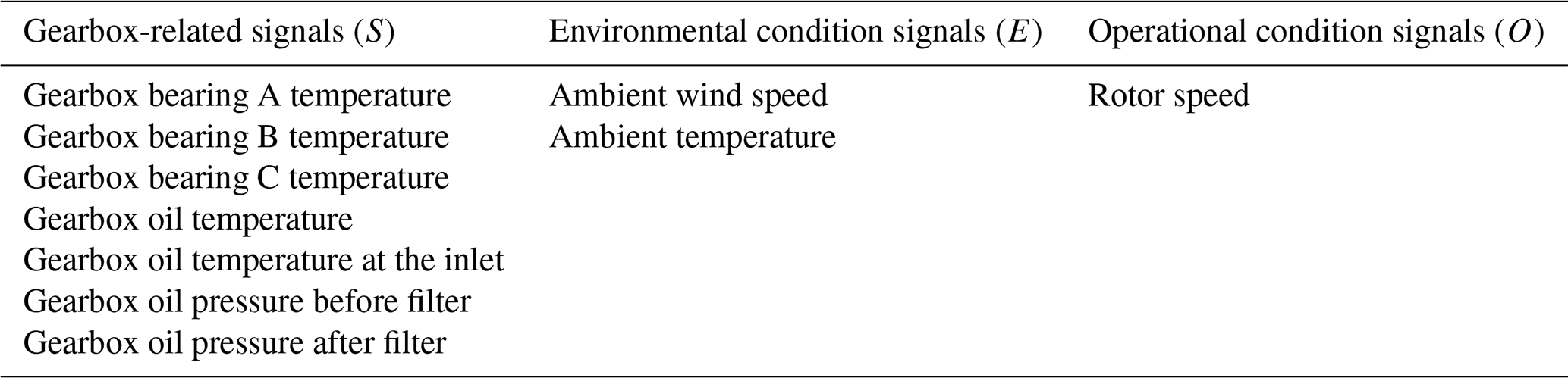
The field dataset used in this work consists of 10 min SCADA signals collected from 1 January 2017 to 1 August 2022 from nine 2 MW wind turbines (WT1–9) in a wind farm operated by Lucky Wind SpA (https://www.luckywind.it/, last access: 6 November 2025). Each turbine has a rotor diameter of 100 m, a hub height of 80 m, and a three-stage gearbox with one planetary stage and two parallel stages. Maintenance logs report that one of the wind turbines, WT8, experienced a gearbox failure on 23 February 2022. Inspection logs report widespread debris indentation and circumferential marks in multiple gearbox bearings and abrasion in several gears. A total of 10 signals are selected for analysis: seven related to gearbox operation, two to environmental conditions, and one to operational conditions. These signals are reported in Table 1. The SCADA signals from WT8 during the year leading to the gearbox failure are used for training purposes. In addition, WT9 data are used as the validation set, and the remaining seven wind turbines are used as the test set.

Table 1 Selected SCADA signals.

3.1 Data preprocessing

Data preprocessing in this study is limited to omitting non-physical signal values and those corresponding to non-operational turbine conditions. Non-physical signal values refer to instances where gearbox-related temperatures are lower than the ambient temperature, gearbox oil pressure is equal to zero, and rotor speed is negative. These outliers, likely caused by sensor malfunctions, constitute around 5 % of the total data. Non-operational values occur when the turbine idles and the produced power is negative. They constitute around 20 % of the total data. As a result, around 25 % of the original data points are excluded from the analysis during the data preprocessing step.

After eliminating these outliers, the signals are resampled into 6 h time intervals. Increasing the sampling period reduces the number of data points, leading to a lower computational burden. It also contributes to a higher signal continuity by reducing the percentage of missing data. However, this comes at the cost of decreased fault detection and RUL prediction accuracy. A 6 h resampling period has been identified as a good trade-off between these factors. As a result, the number of data points in a year drops from around 52 000 to around 1400, and the percentage of missing data decreases from around 25 % to around 3 %.

4 Fault detection case study

In this section, an experiment is performed to assess the effectiveness of the developed synthetic data generation method in fault detection by comparing the detection performance with and without synthetic data. A classifier is trained with the training (WT8) signals spanning 23 February 2021 to 23 February 2022 (the gearbox failure time) to identify faulty gearbox operation. The timestamps during the last month before failure are labelled as faulty (1), while the remaining 11 months is labelled as healthy (0). Selecting a smaller portion of data as the faulty class can reduce false positives. However, it leads to a higher data imbalance and can reduce model performance. In this work, the length of 1 month constitutes the minimum length of the faulty training data that maintain an acceptable level of data imbalance, allowing for successful training of the fault detection model.

Figure 5 Applying a rolling time window of length w to the condition time series.

The classifier used is an artificial neural network (ANN) with three hidden layers consisting of 16, 8, and 4 neurons, each with a ReLU activation function. The output layer uses a sigmoid activation function. The model is trained using the Adam optimiser (Kingma and Ba, 2014) with its default parameters and the binary cross-entropy loss function (Goodfellow et al., 2016). During training, a training–validation split is performed, where 20 % of the training data are randomly set aside for validation, and the training is stopped when the validation loss stops decreasing for 20 consecutive epochs. The model architecture is set using trial and error, where the model complexity is gradually increased in terms of the number of hidden layers and neurons per layer, until a significant performance improvement is not observed in the validation set. Because of the highly imbalanced nature of the number of healthy and faulty data points in the training set with the minority (faulty) class encompassing only 8.3 % of the data points, the SMOTE method (Chawla et al., 2002) has been used to oversample the faulty data points and balance the two classes. The shape of the training data before and after SMOTE oversampling is shown in Fig. 6.

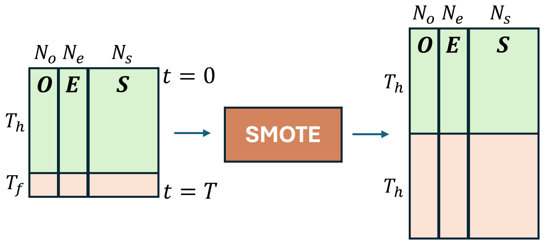
Figure 6 Flowchart of the SMOTE oversampling. T_h and T_f refer to WT8 time frames labelled as healthy and faulty. They span 11 months and 1 month, respectively.

Once trained, the ANN is used to predict fault state labels (0 or 1) for each timestamp in the SCADA signals of WT1–7 and WT9. State change from healthy to faulty is generally a gradual rather than instantaneous process. Therefore, an individual timestamp predicted as faulty might be due to noise rather than an actual fault (Zhao et al., 2017). For this reason, in Zhao et al. (2017) and Peter et al. (2022), the ratio of the detected anomalous data points to the total number of data points within a fixed time window is used as a fault index. In this work, a similar approach is adopted. A fault index is defined as the weekly moving average (MA) of the predicted labels to improve detection robustness. The flowchart of the fault detection methodology is shown in Fig. 7. The results for the training wind turbine and three test wind turbines are shown in Fig. 8a–d. Numerous misclassified labels, i.e., a predicted label of 1 when the gearbox is healthy, are observed mainly for WT2 in Fig. 8b and WT7 in Fig.8d, particularly clustered around February each year, which coincides with the failure month of WT8, used to train the ANN. This suggests that, due to the availability of only one failure event for training, the ANN has learnt the seasonal features in the signals around the failure time of WT8, associating these features with class 1 (faulty).

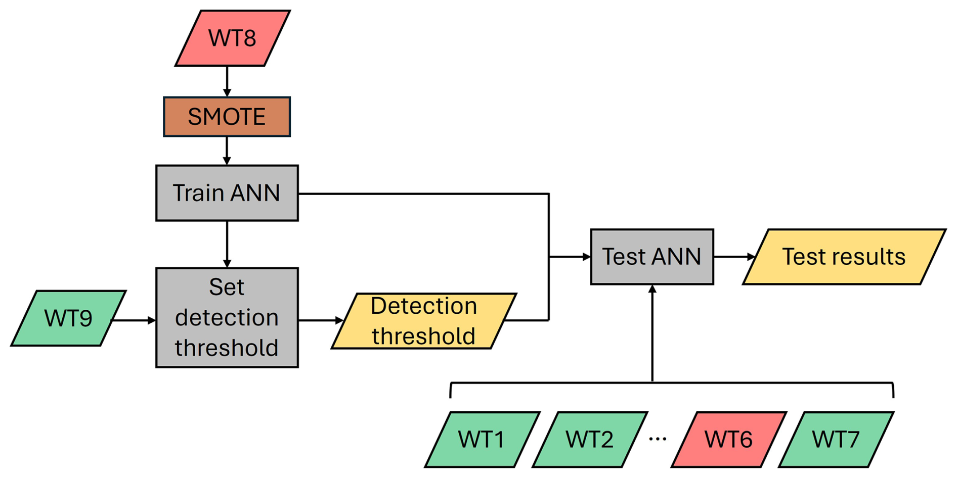
Figure 7 Flowchart of the fault detection without synthetic datasets. The red blocks represent faulty wind turbine data, and the green blocks represent healthy wind turbine data.

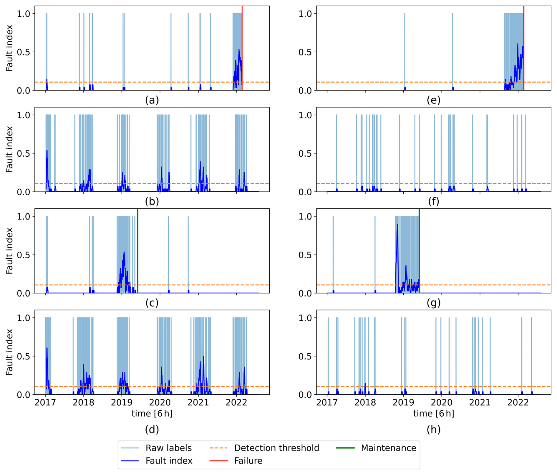
Figure 8 Predicted raw labels and their weekly moving average (fault index): (a–d) obtained with the original signals and (e–h) with both original and synthetic signals. Panels (a) and (e) refer to the training wind turbine (WT8), (b) and (f) to WT2 (healthy), (c) and (g) to WT6 (faulty), and (d) and (h) to WT7 (healthy).

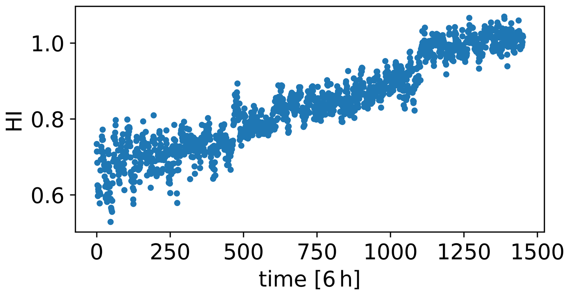
To address this problem, the developed cGAN-based framework is used to generate synthetic signals that simulate the degradation and failure of the WT8 gearbox across various time frames. To create the condition time series C, an HI is built using the proposed HI construction method, representing the degradation of the WT8 gearbox during the year leading to its failure. The obtained HI is shown in Fig. 9. This HI and the three environmental and operational condition signals of WT8 form the condition time series (N_c=4). These, along with the seven gearbox-related signals of WT8 (N_s=7), are used to train the cGAN. The Adam optimiser is used with a learning rate of 0.0005 to train both the generator and the discriminator. This learning rate is lower than the default 0.001 value. Due to the complexities arising from coupling two neural networks within a single training process, this lower learning rate is required to ensure training stability.

Figure 9 HI of WT8 during the year leading to the gearbox failure.

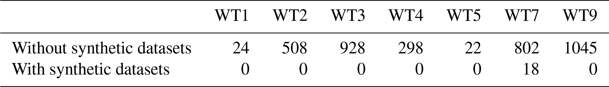
Once the cGAN is trained, the environmental (E) and operational (O) condition signals are shifted from the February 2021–February 2022 time frame to new time frames, April 2020–April 2021, July 2019–July 2020, September 2018–September 2019, and December 2017–December 2018, while keeping the degradation signal (D) unchanged. These time frames are selected to simulate the gearbox failure in a variety of seasonal conditions. This results in four new condition time series ${\mathbf{C}}_i=\mathit{\{}{\mathbf{O}}_i,{\mathbf{E}}_i,D\mathit{\}}$, where $i=\mathrm{1},\mathrm{\dots },\mathrm{4}$. These condition time series are then input to the trained generator, which generates the corresponding synthetic signal time series ${\mathbf{S}}_i^s$, where $i=\mathrm{1},\mathrm{\dots },\mathrm{4}$. Together with their corresponding environmental and operational signals (E and O), these synthetic signal time series form four synthetic SCADA datasets. Similar to the original dataset, the initial 11 months in the synthetic datasets is labelled as healthy, while the last month leading to failure is labelled as the faulty class and is oversampled using SMOTE to balance the two classes. The test set predictions using the ANN trained with both the original and the synthetic datasets are shown in Fig. 8e–h for the training wind turbine and three test wind turbines. A noticeable decrease in the number of misclassified labels can be observed when compared to the predictions made using only the original dataset. Across the wind turbines in the healthy test and validation sets, the number of misclassified labels, reported in Table 2, has decreased significantly, by around 84 % on average. A detection threshold of 0.107 is selected for the fault index based on the maximum fault index value observed in the validation wind turbine, the crossing of which indicates a fault. False positives, i.e., the timestamps when the fault index is above the detection threshold while the gearbox is healthy, are reported in Table 3 and have been almost completely resolved. It is important to note that the number of false positives depends on the detection threshold, which is set based on the randomly selected validation wind turbine (WT9). The component temperatures in different wind turbines can have slight differences in the healthy state. This results in a variability in the number of misclassified labels in different healthy wind turbines reported in Table 2. Therefore, selecting a different wind turbine for validation can change the number of false positives slightly by lowering or raising the detection threshold. However, this affects the number of false positives similarly in the two cases with and without synthetic datasets. Therefore, this experiment is a valid tool for performance comparison. The flowchart of the fault detection methodology with the synthetic datasets is shown in Fig. 10.

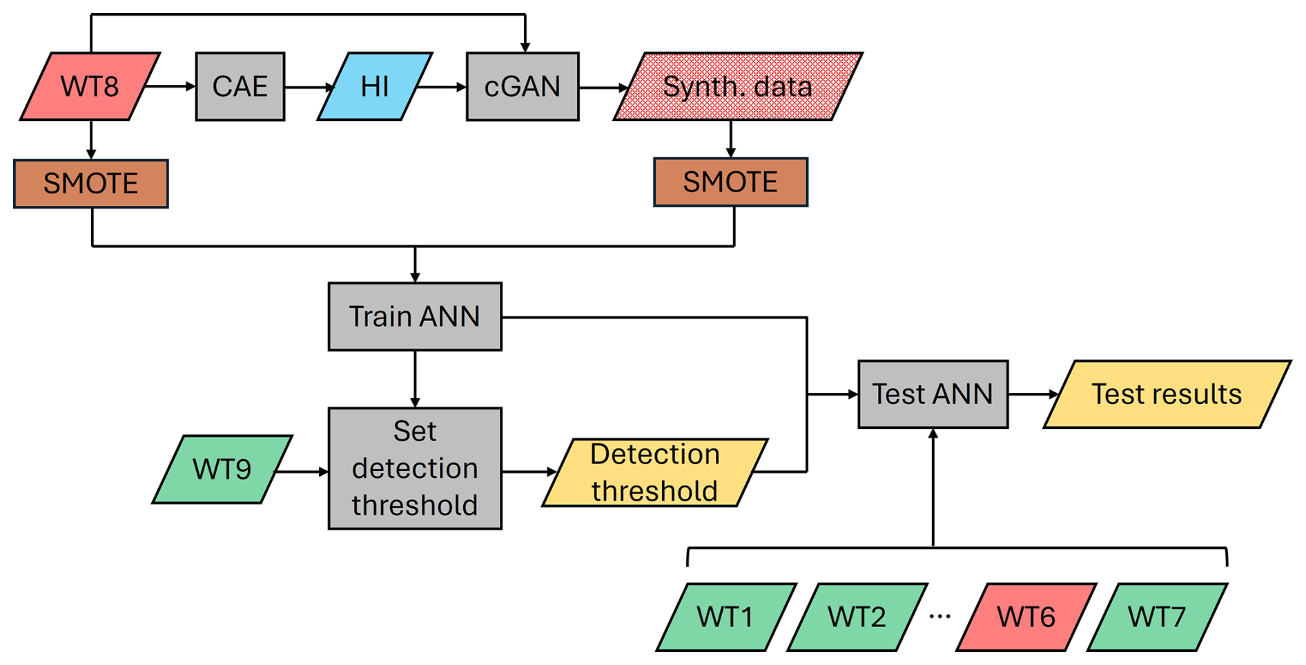
Figure 10 Flowchart of the fault detection with synthetic datasets. The red blocks represent faulty wind turbine data, and the green blocks represent healthy wind turbine data.

The results show a clear detection of a potential anomaly and fault in WT6. The fault index increases sharply around the end of October 2018 and remains at a lower level until around the end of May 2019. Further investigation into the farm maintenance logs and monthly reports revealed that a moderate gearbox-related fault was discovered and addressed during a 12 h maintenance intervention on 30 May 2019. Coincidentally, this anomaly occurred during the seasonal period where false positives were previously observed in Fig. 8a–d. Therefore, without the synthetic data, detecting this fault with high certainty would have been challenging.

Considering the detection threshold of 0.107, the fault in WT6 is detected on 19 October 2018 at 06:00:00, more than 7 months before the maintenance. Furthermore, the fault in WT8 is detected on 28 August 2021 at 06:00:00, as shown in Fig. 8e, while the actual failure occurred on 23 February 2022.

Table 2 Number of misclassified labels in the healthy test and validation set wind turbines.

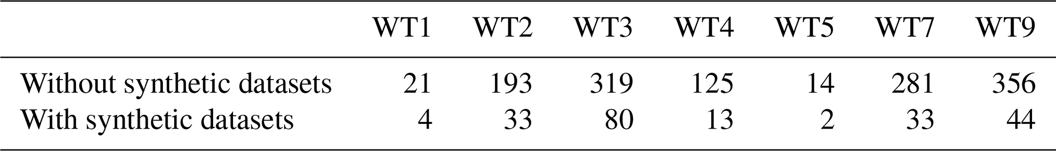
Table 3 Number of false positives in the healthy test and validation set wind turbines.

5 RUL prediction case study

This section assesses the effectiveness of the developed method in fault prognosis. WT8, used for training, experienced a gearbox failure, while WT6's gearbox underwent maintenance while the fault was at a moderate level, and failure did not occur. As a result, a ground truth failure time is not available for the gearbox of WT6. For this reason, the fault prognosis in this section aims to predict the time when the degradation reaches a level that can be detected by the fault detection method discussed in the previous section.

The CAE used for HI construction is trained with WT8 signals spanning the year leading to the gearbox failure. A threshold of 1 is assigned for gearbox failure, as indicated by the f₁ term in the CAE training fitness function in Eq. (3). Additionally, the mean value of the HI during the week leading to the detection in WT8, which is 0.84, is set as the HI threshold corresponding to the degradation level associated with the fault detection. Figure 11 shows WT8 HI along with these thresholds. Using the trained CAE, the WT6 HI is then constructed and is shown in Fig. 12a.

Figure 11 HI of WT8 and the selected thresholds for detection and failure.

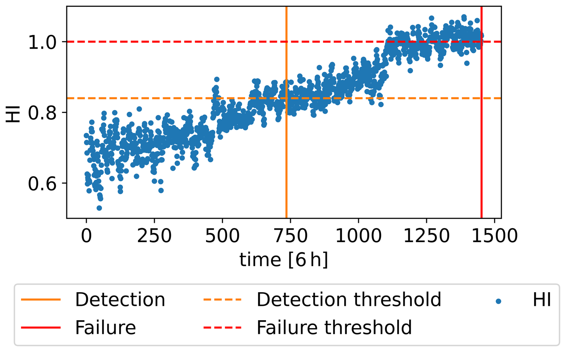
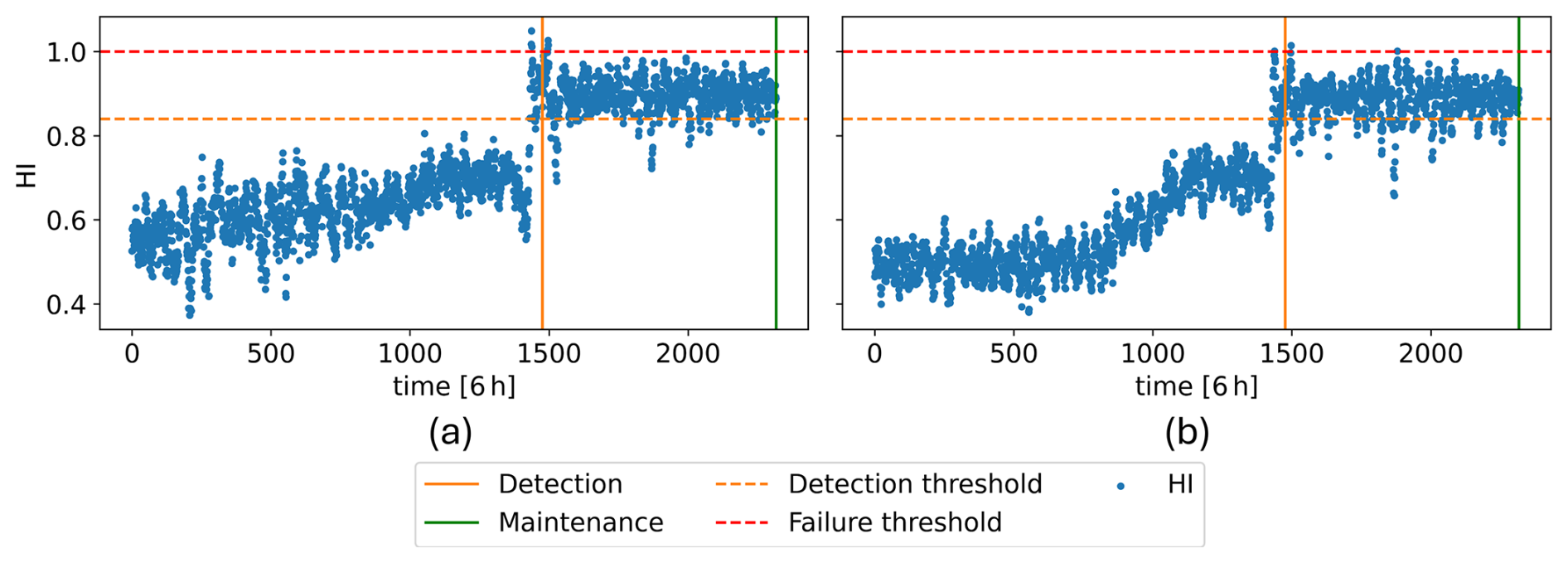
Figure 12 WT6 HI: (a) with the original signals and (b) with both original and synthetic signals (b).

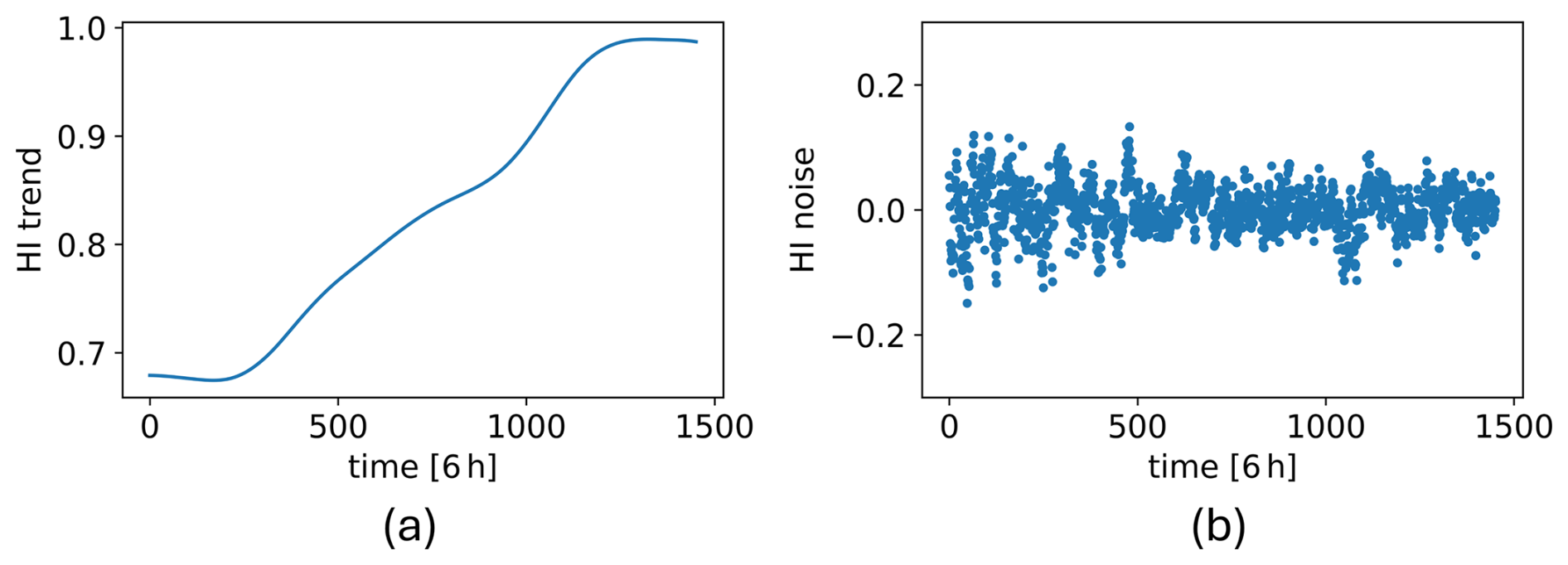
To properly train the CAE to extract the true degradation trend, a training set comprising multiple run-to-failure datasets with diverse degradation trajectories is needed. To achieve this, synthetic signals are generated by modifying the degradation trend D in the condition time series C and shifting the environmental E and operational O signals. The resulting four new condition time series, then, become ${\mathbf{C}}_i^{\prime }=\mathit{\{}{\mathbf{O}}_i,{\mathbf{E}}_i,D_i\mathit{\}}$, where $i=\mathrm{1},\mathrm{\dots },\mathrm{4}$, with $D_{\mathrm{1}},\mathrm{\dots },D_{\mathrm{4}}$ representing four different degradation trajectories. To derive $D_{\mathrm{1}},\mathrm{\dots },D_{\mathrm{4}}$, the Complete Ensemble Empirical Mode Decomposition with Adaptive Noise (CEEMDAN) algorithm (Colominas et al., 2014) is applied to decompose the training HI in Fig. 9 into its trend component D_trend and several other intrinsic mode functions (IMFs), D_IMF,i, which collectively make up the HI noise.

$$\begin{array}{}\text{(12)}& {\displaystyle }D=D_{\mathrm{trend}}+D_{\mathrm{noise}}\text{(13)}& {\displaystyle }{D}_{\mathrm{noise}}=\sum _{i=\mathrm{1}}^{N_{\mathrm{IMF}}}{D}_{\mathrm{IMF},i}\end{array}$$

Here N_IMF is the number of IMFs other than the trend. The decomposed trend and noise components of the training HI are shown in Fig. 13.

Figure 13 Decomposition of the WT8 HI into the (a) trend and (b) noise component.

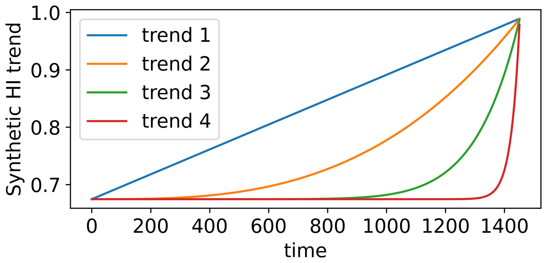
Then, four synthetic trends are created using the equation below:

$$\begin{array}{}\text{(14)}& \begin{array}{rl}{D}_{\mathrm{trend},i}\left(t\right)& =min\left(D_{\mathrm{trend}}\right)+[max\left(D_{\mathrm{trend}}\right)\\ & -min\left(D_{\mathrm{trend}}\right)]{\left({\displaystyle \frac{t}{T}}\right)}^{p_i},i=\mathrm{1},\mathrm{\dots },\mathrm{4},\end{array}\end{array}$$

with p₁₋₄ equal to 1, 3, 10, and 50, respectively, and are plotted in Fig. 14. This equation models an HI trend starting at the minimum value of the WT8 HI trend and ending at its maximum value. It is important to note that assigning a fixed HI value at failure time for all synthetic HIs is valid in the proposed framework, as the model used for HI construction is explicitly trained to associate failure with an HI value of 1. This enforces consistency by design and minimises variability in the HI at failure across different realisations. The exponent p_i determines the trend regime. A value of 1 produces a linear trend, while higher values indicate more pronounced non-linearity, representing increasingly abrupt degradation patterns. The p₁₋₄ values are chosen to represent meaningfully distinct degradation behaviours.

Figure 14 Four degradation trends used to obtain the synthetic HIs.

Next, the corresponding synthetic HIs are obtained by adding the WT8 HI noise to the synthetic trends and are shown in Fig. 15. These, combined with the shifted operational and environmental signals, form the four new condition time series ${\mathbf{C}}_{\mathrm{1}}^{\prime },\mathrm{\dots },{\mathbf{C}}_{\mathrm{4}}^{\prime }$, which are fed into the trained generator to obtain their respective synthetic signal time series ${\mathbf{S}}_{\mathrm{1}}^{s^{\prime }},\mathrm{\dots },{\mathbf{S}}_{\mathrm{4}}^{s^{\prime }}$. These synthetic signals, along with the corresponding E and O signals, create four additional synthetic datasets that are added to the CAE's training set. Subsequently, an HI is constructed for WT6, which is shown in Fig. 12b.

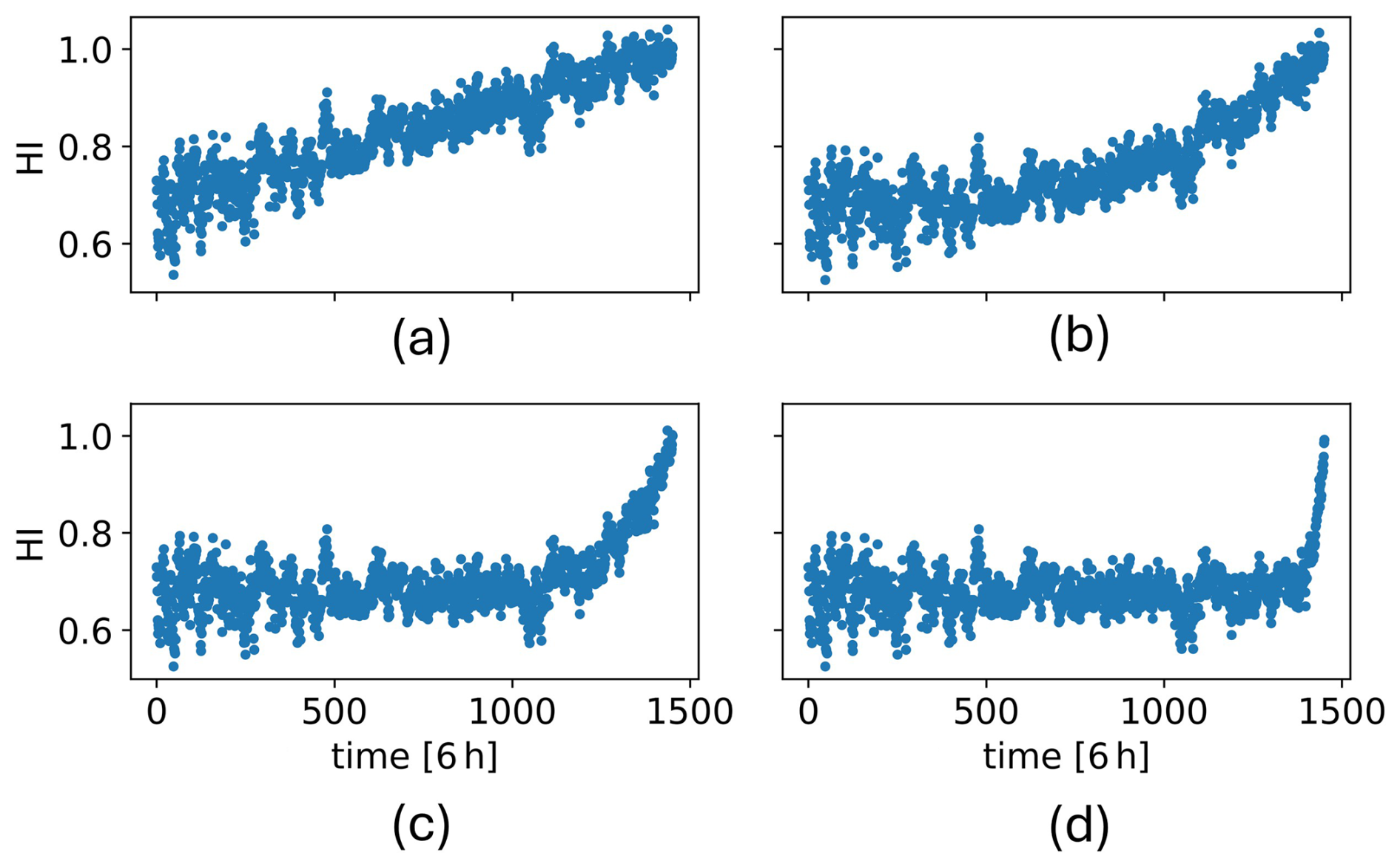
Figure 15 Synthetic HIs used to generate the synthetic signals: (a–d) refer to HI1–4 built with trends 1–4.

Regardless of the inclusion of synthetic datasets, the HI built for WT6 crosses the detection threshold around the time the gearbox fault is detected and briefly overshoots the failure threshold. However, this exceedance is not sustained, and the HI stabilises between the detection and failure thresholds until the fault is identified and addressed through maintenance, preventing complete failure. These results align well with the behaviour of the fault index in Fig. 8g and the WT6 maintenance report, which confirms a moderate gearbox-related fault. The sudden jump observed both in the fault index and the HI might be due to a sudden fault, such as a crack. However, this hypothesis cannot be asserted with confidence, since no in-depth details are available about this fault case.

Notably, the HI built using synthetic datasets exhibits a clearer degradation trend, achieving a monotonicity of 0.61 (measured by the MK metric) up to the detection point compared to 0.53 when synthetic datasets are not used.

To assess the performance of the two HIs in Fig. 12a and b in predicting the RUL up to the detection point, a second-order polynomial function $a{t}^{\mathrm{2}}+bt+c$ is fitted to the HI up to timestamp t with $t=\mathrm{700},\mathrm{\dots },\mathrm{1470}$ (detection time) in 6 h units. The projected crossing point of the fitted function with the detection threshold of 0.84 is then used to calculate the predicted RUL at each t. To ensure convexity and guarantee that the projected trend crosses the threshold, the constraint a≥0 is enforced during curve fitting. This approach can model both linear and curved trends, using the fewest parameters possible, minimising the risk of overfitting. The true and predicted RULs are shown in Fig. 16. At each timestamp, the true RUL corresponds to the number of 6 h timestamps remaining until the detection time. It can be seen that the HI built with the synthetic datasets considerably outperforms the one built without them in correctly predicting the RUL. Considering an error bound of 1 month, this HI achieves a prognosis horizon of around 4.5 months. This implies that using this HI, along with the adopted RUL prediction approach, enables consistent fault time prediction with the assigned accuracy up to 4.5 months in advance. It is worth noting that a simple RUL prediction approach is used in this work, as developing more complex forecasting approaches is beyond the scope of this work. Adopting more sophisticated approaches could lead to even better RUL prediction performance.

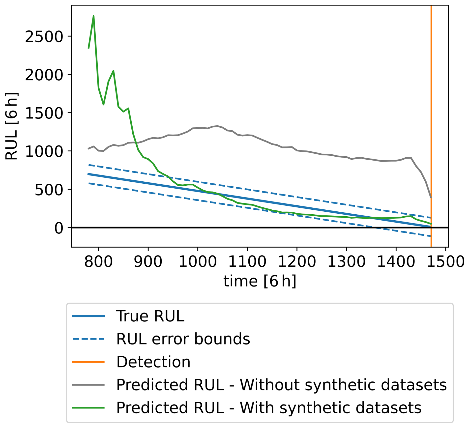
Figure 16 Comparison between the WT6 true and predicted RULs during the year leading to the fault detection.

6 Conclusions

In this work, a method based on cGANs is developed to generate synthetic SCADA signals. This approach enables the generation of sensor time series with controllable degradation trends, as well as operational and environmental conditions. As a result, it can simulate new failure events or recreate a given failure under different conditions. A fault detection case study demonstrates that this method almost completely resolves false positives. This allows for the blind detection of a fault in one of the test wind turbines more than 7 months before it was discovered and maintained by the wind farm operators. The false positives are due to the availability of only one failure event in the training data, leading the model to associate the seasonal characteristics of signals at the time of failure with fault features. By augmenting the training data with synthetic signals that simulate the same failure under different seasonal conditions, this problem is mitigated. Furthermore, the study shows that training an HI construction method with synthetic signals simulating diverse degradation scenarios leads to a considerably more accurate RUL prediction. This approach enables the prediction of the RUL up to 4.5 months before fault detection in a test wind turbine. In contrast, the HI built without synthetic signals fails to provide accurate RUL estimates.

It is important to note that the training and test fault cases in this work are similar, both involving a fault in the gearbox that led to elevated temperatures in the gearbox-related SCADA signals. Therefore, the method's performance might deteriorate if the test failure mode is significantly different from the training case. This work serves as a feasibility analysis that proves the proposed approach can generate entire sets of time series simulating new failure events that are able to mitigate the overfitting problem. To identify the extent of diversity in the failure patterns that can be simulated using this method and assess its performance in the presence of various failure modes, further studies and experiments with multiple failure cases are required.

Accurately forecasting the future trajectory of an HI for RUL prediction remains an important topic that is out of the scope of this paper. Therefore, a simple prediction approach is employed. This approach can perform well when the degradation trend remains consistent throughout the lifetime of the component. However, it can fail in the presence of inconsistent and complex trends. Future research will focus on developing probabilistic approaches for more precise RUL prediction using component HIs.