Gulf of Mexico hurricane hazard assessment for offshore wind energy sites

A feasibility assessment of offshore wind in the Gulf of Mexico conducted by the National Renewable Energy Laboratory concluded that hurricane risk was one of the major challenges that would need to be overcome for a mature offshore wind industry to develop in the Gulf of Mexico, as the hurricanes that frequent this area can potentially exceed design limits prescribed by the International Electrotechnical Commission (IEC) wind design standards. To better understand and account for these unique conditions, we target two objectives. The first is to develop a translation between the well-established Saffir–Simpson hurricane scale and the IEC design classes, which are based upon different averaging periods and reference heights and often lead to misinterpretation, speculation, and uncertainty. The conversion of wind speed averaging times between Saffir–Simpson and IEC design standards reflects the behaviour of the sea surface drag coefficient as a function of the mean wind speed, which controls the turbulence characteristics of the hurricane boundary layer near the surface. The second objective is to quantify the hurricane exposure risk for wind turbines at sites potentially impacted by hurricanes in the Gulf of Mexico using probabilistic hurricane track and wind field models. The IEC prescribes the reference wind speeds associated with Class 1A and Typhoon Class limit states to be 50 years, though model results indicate the return periods associated with the IEC Class 1A limit state range from approximately 20 to 45 years, while the return periods associated with the Typhoon Class limit state range from approximately 40 to 110 years. Ultimately, this indicates that the Class 1A limit state may be nonconservative for the entire Gulf of Mexico offshore wind energy area, while the Typhoon Class limit state may be adequate for the design of turbines in some regions of the Gulf of Mexico offshore wind energy area.

1 Introduction

To ensure the robust design of wind turbines in the Gulf of Mexico, it is critical to understand the added risk posed by the threat of major hurricanes, as those affecting the Gulf of Mexico region have significant potential to exceed design limits prescribed by the International Electrotechnical Commission (IEC) wind design standards. In the last decade alone, five hurricanes (Harvey 2017, Sally 2020, Delta 2020, Zeta 2020, and Ida 2021) have produced wind speeds off the U.S. Gulf Coast that exceeded the IEC Class 1A and Typhoon Class reference wind speeds according to the National Hurricane Center (NHC) Atlantic Basin Best Track Data, hereafter HURDAT2 (Landsea and Franklin, 2013). Extreme wind speeds and wave heights associated with these major hurricanes in the Gulf of Mexico could cause severe damage or total failure of offshore wind turbines and their components. Existing U.S. offshore wind farms are currently only located along the northern Atlantic seaboard and do not provide a robust catalogue of information on the performance of wind turbines during such events. However, offshore wind farms in the northwest Pacific Ocean, the most active tropical cyclone basin in the world and where the offshore wind energy industry is more mature, do provide a longer history of performance of wind turbines subjected to typhoons. Since the early 2000s, six typhoons have caused structural failures of wind turbines across seven different wind farms in China, with the main failure modes attributed to severe blade damage, buckling of the support tower, and foundation overturning (Li et al., 2022). To overcome a lack of observational data for wind turbines exposed to tropical cyclones in other regions, many studies have been performed using finite element models, probabilistic models, physics-based simulations, and performance-based engineering (Lipari et al., 2024). In one such study, the return period associated with damaging hurricane wind speeds, defined as surface-level mean wind speeds exceeding 50 m s⁻¹ (111.9 mph), in the Gulf of Mexico was estimated to be as low as 8 years (Mattu et al., 2022).

To satisfy this charge, this paper defines the wind hazard for the Gulf of Mexico offshore wind energy area using the hurricane hazard model developed by Applied Research Associates and published extensively in the open literature (Vickery et al., 2000a, b, 2009a, b; Vickery, 2005; Vickery and Skerlj, 2005; Vickery and Wadhera, 2008). In doing so, the return periods associated with the IEC Class 1A and Typhoon Class limit-state hurricanes are estimated on a grid with a nominal resolution of 10 km to determine where hurricane risk results in the exceedance of the IEC design criteria. On the same grid, wind speed hazard contours associated with return periods of 50 and 500 years are also estimated.

An additional challenge in assessing hurricane wind speed risk in the Gulf of Mexico arises from inconsistent terminology across the Saffir–Simpson hurricane scale and the IEC design criteria. Saffir–Simpson definitions are based on 1 min sustained wind speeds estimated at a 10 m height over marine terrain, while the IEC uses a different averaging period (3 s versus 1 min) and reference height (assumed herein to be a hub height of 150 versus 10 m). Employing the latest research on turbulence characteristics of the hurricane boundary layer, conversions between various durations (e.g. 3 s, 1 min, 10 min, 1 h) and between elevations near the surface (10 m) to near hub height (assumed herein to be 150 m) are developed. IEC Class 1A and Typhoon Class limit states are also provided in terms of an equivalent Saffir–Simpson hurricane wind speed category.

2 Harmonizing hurricane terminology for offshore wind design

Wind speeds specified in various design codes and those reported by the U.S. Weather Service are often associated with different averaging times. For example, the IEC specifies a 10 min average wind speed over an open water surface, whereas the U.S. wind loading standard, American Society of Civil Engineers (ASCE) 7, specifies a 3 s gust wind speed over open land, and the U.S. Weather Service specifies a 1 min average wind speed, where, in the case of a hurricane, the wind speed is usually associated with an open water terrain. In all cases, the specified wind speeds are at a height of 10 m. In the case of hurricanes, the conversion is wind speed dependent, as the surface roughness and turbulence characteristics vary with wind speed, whereas the conversion factors vary with height in all cases. Here, we present an approach for converting a wind speed specified with one averaging time to another averaging time to allow better comparisons between IEC wind turbine standards and the Saffir–Simpson hurricane categories.

The conversion of wind speed averaging times from one averaging time to another (e.g. from a 1 min average to a 3 s gust) requires information on the turbulence characteristics of the hurricane boundary layer. The relevant turbulence characteristics are the turbulence intensity and the velocity spectrum, both of which, near the surface, depend only on height and the surface roughness. The surface roughness is a function of the mean wind speed and the surface drag coefficient. In addition to controlling the turbulence characteristics of the wind, the sea surface drag coefficient also controls the vertical shear, or the rate of change of wind speed with height. The behaviour of the surface drag coefficient as a function of wind speed and wave parameters has received significant attention since the pioneering study by Powell et al. (2003). Powell et al. (2003) showed that the drag coefficient reaches a maximum for mean wind speeds at a height of 10 m above mean sea level (m a.m.s.l.) (U₁₀) in the range of 20 to 30 metres per second (m s⁻¹) and then decreases with increasing wind speed. Here, we review many of the studies examining the sea surface drag coefficient published since 2003 to determine the model that best describes the behaviour of the sea surface drag coefficient as a function of the mean wind speed.

2.1 Sea surface drag coefficient

The sea surface drag coefficient in Powell et al. (2003) was developed by computing the variation of the mean wind speed with height over the lower 500 m of the hurricane boundary layer and then fitting the results of the lower 100 to 200 m with a logarithmic boundary layer model, from which the aerodynamic surface roughness is obtained. The profiles were grouped into 10 m s⁻¹ “bins”, based on the mean wind speed averaged over the lowest 500 m. Wind speeds were obtained from Global Positioning System (GPS) dropsondes falling through the boundary layer. Details on the computation of wind speeds from dropsondes are given in Hock and Franklin (1999). In addition to Powell et al. (2003), the dropsonde and mean velocity profile approach, or flux-profile method, has been used by Vickery et al. (2009a), Holthuijsen et al. (2012), Richter et al. (2016), and Ye et al. (2022).

Assuming a logarithmic profile, the variation of the mean wind speed with height, U(z), is given as

$$\begin{array}{}\text{(1)}& U\left(z\right)={\displaystyle \frac{u_{\ast }}{k}}\ln \left({\displaystyle \frac{z}{z_{\mathrm{0}}}}\right),\end{array}$$

where u_∗ is the friction velocity, k is the von Karmen constant (k=0.4), z is height, and z₀ is the aerodynamic surface roughness. From Eq. (1), it is seen that, at z=z₀, the mean wind speed equals 0. The surface shear stress, τ₀, is defined as

$$\begin{array}{}\text{(2)}& {\mathit{\tau }}_{\mathrm{0}}=\mathit{\rho }{u}_{\ast }^{\mathrm{2}}=\mathit{\rho }{C}_{{\mathrm{d}}_{\mathrm{10}}}{U}_{\mathrm{10}}^{\mathrm{2}},\end{array}$$

where $C_{{\mathrm{d}}_{\mathrm{10}}}$ is the sea surface drag coefficient with respect to U₁₀. Combining Eqs. (1) and (2) yields

$$\begin{array}{}\text{(3)}& C_{{\mathrm{d}}_{\mathrm{10}}}={\left[k/\ln \left({\displaystyle \frac{\mathrm{10}}{z_{\mathrm{0}}}}\right)\right]}^{\mathrm{2}}.\end{array}$$

Thus, given z₀, it is straightforward to compute $C_{{\mathrm{d}}_{\mathrm{10}}}$. Examples of profiles fitted to the logarithmic profile to estimate z₀ are shown in Fig. 1.

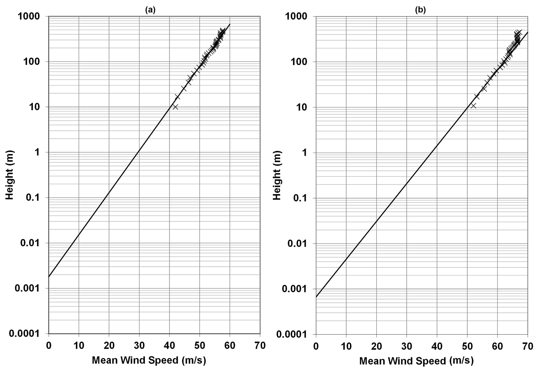
Figure 1 Example measured and fitted velocity profiles. Profiles fitted using the method of least squares over a height range of 20 to 150 m. Computed surface roughnesses in these examples are 0.0018 and 0.00067 m for the left (a) and right plots (b), respectively. Plots derived using the same data used in Vickery et al. (2009a) and comprise an average of many drops from many hurricanes in the Gulf of Mexico and the Atlantic Ocean.

Figure 2 presents a plot of $C_{{\mathrm{d}}_{\mathrm{10}}}$ vs. U₁₀ obtained from the data given in Powell et al. (2003), Vickery et al. (2009a), Holthuijsen et al. (2012), Richter et al. (2016), and Ye et al. (2022) showing $C_{{\mathrm{d}}_{\mathrm{10}}}$ increasing with wind speed, reaching a maximum at a mean wind speed of 37 m s⁻¹ and then decreasing with further increases in wind speed.

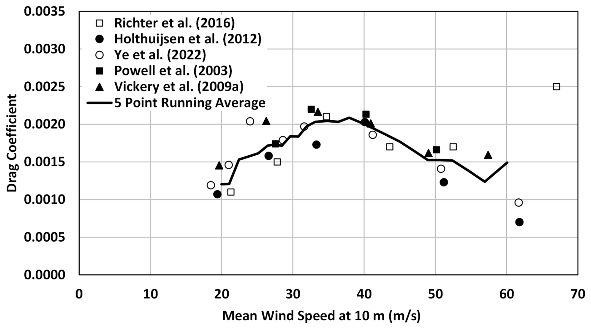
Figure 2 Variation of $C_{{\mathrm{d}}_{\mathrm{10}}}$ in tropical cyclones with mean wind speed from various studies obtained using the flux-profile method using GPS dropsondes plotted vs. U₁₀.

Gao et al. (2021), using an eddy-covariance method with data from aircraft flying through tropical cyclones, suggests that $C_{{\mathrm{d}}_{\mathrm{10}}}$ reaches a maximum of $\mathrm{1.20}\times {\mathrm{10}}^{-\mathrm{3}}$ at a saturation wind speed of 33.5 m s⁻¹. However, the maximum wind speed in their data is only 28 m s⁻¹, and the saturation wind speed of 33.5 m s⁻¹ was determined using the results of other studies. Vickers et al. (2013) also used aircraft eddy-covariance measurements to determine the relationship between $C_{{\mathrm{d}}_{\mathrm{10}}}$ and wind speed and found that $C_{{\mathrm{d}}_{\mathrm{10}}}$ reaches a maximum of about $\mathrm{2.3}\times {\mathrm{10}}^{-\mathrm{3}}$ at a mean wind speed of about 19 m s⁻¹. The data show a decrease in $C_{{\mathrm{d}}_{\mathrm{10}}}$ as the wind speed increases beyond 19 m s⁻¹, but the maximum wind speed is only 23 m s⁻¹.

Laboratory studies performed by Takagaki et al. (2012) suggest that the drag coefficient reaches a maximum of about $\mathrm{2.58}\times {\mathrm{10}}^{-\mathrm{3}}$ for wind speeds greater than about 33 m s⁻¹. Donelan et al. (2004), also using laboratory studies, found that $C_{{\mathrm{d}}_{\mathrm{10}}}$ reaches a maximum of about $\mathrm{2.5}\times {\mathrm{10}}^{-\mathrm{3}}$ at U₁₀= 33 m s⁻¹. Note that Curcic and Haus (2020) found an error in the computer code used in the Donelan et al. (2004) paper, changing the saturation speed from 33 to 29 m s⁻¹ and increasing the limiting value of $C_{{\mathrm{d}}_{\mathrm{10}}}$ from $\mathrm{2.5}\times {\mathrm{10}}^{-\mathrm{3}}$ to $\mathrm{3.0}\times {\mathrm{10}}^{-\mathrm{3}}$. Troitskaya et al. (2012) also performed laboratory studies indicating that the drag coefficient reaches a maximum of about $\mathrm{2.5}\times {\mathrm{10}}^{-\mathrm{3}}$, but for U₁₀ of about 50 m s⁻¹. Lee et al. (2022) suggest that laboratory experiments cannot be used to determine $C_{{\mathrm{d}}_{\mathrm{10}}}$ because the effects of wave age, fetch, wavelength, and sea spray are not modelled.

Using data from both laboratory and full-scale experiments, Donelan (2018) suggests that, in addition to a wind speed dependence, $C_{{\mathrm{d}}_{\mathrm{10}}}$ is a function of the wind–sea Reynolds number, R_B, and wave age and that the reduction in drag coefficient above 30 m s⁻¹ is largely associated with a wave sheltering effect, where a downstream trough is sheltered by flow separation at the crest of a wave, thereby reducing the skin stress in the wave trough. The wind–sea Reynolds number, R_B, is defined as

$$\begin{array}{}\text{(4)}& R_B={\displaystyle \frac{u_{\ast }^{\mathrm{2}}}{{\mathit{\omega }}_{\mathrm{p}}\mathit{\upsilon }}}={\displaystyle \frac{T_{\mathrm{s}}{u}_{\ast }^{\mathrm{2}}}{\mathrm{2}\mathit{\pi }\mathit{\upsilon }}},\end{array}$$

where υ is the kinematic viscosity of sea water and T_s is the significant wave period. Wave age, β, is defined as

$$\begin{array}{}\text{(5)}& \mathit{\beta }={\displaystyle \frac{c_{\mathrm{p}}}{U_{\mathrm{10}}}},\end{array}$$

where c_p is the phase speed of the waves. In deep water, c_p is obtained from

$$\begin{array}{}\text{(6)}& c_{\mathrm{p}}={\displaystyle \frac{g}{\mathit{\omega }}}={\displaystyle \frac{g{T}_{\mathrm{s}}}{\mathrm{2}\mathit{\pi }}}.\end{array}$$

Hsu et al. (2019) also suggest that $C_{{\mathrm{d}}_{\mathrm{10}}}$ is a function of the waves, specifically suggesting that $C_{{\mathrm{d}}_{\mathrm{10}}}$ is a function of the parameter ζ, defined as

$$\begin{array}{}\text{(7)}& \mathit{\zeta }={\displaystyle \frac{gT}{\left|U_{\mathrm{10}}\right|\cos \mathit{\delta }}}={\displaystyle \frac{g\left(\frac{\mathit{\chi }}{U_{\mathrm{h}}}\right)}{\left|U_{\mathrm{10}}\right|\cos \mathit{\delta }}},\end{array}$$

where g is the acceleration due to gravity, T is the duration the wind blows over a fetch of length χ, δ is the angle between $\left|U_{\mathrm{10}}\right|$ and the surface waves, and U_h is the translation speed of the hurricane.

Smith and Montgomery (2010, 2014) argue that the log-law does not apply within the eyewall of a hurricane. Consequently, the computation of an effective surface roughness using the approach used in Powell et al. (2003) and others is not valid.

Ye et al. (2022) used the profile method to examine the behaviour of $C_{{\mathrm{d}}_{\mathrm{10}}}$ at high wind speeds, focusing on the region near the radius to maximum winds (RMW). They found the same reduction in $C_{{\mathrm{d}}_{\mathrm{10}}}$ with wind speeds found in other studies using the profile method, but they postulated that tropical cyclone dynamics play a role in affecting the validity of the profile method, e.g. as in Smith and Montgomery (2014). Richter et al. (2021), like Smith and Montgomery (2014), conclude that the flux-profile method may not be valid near the eyewall, suggesting that the flux-profile approach leads to an underestimate of the true value of $C_{{\mathrm{d}}_{\mathrm{10}}}$. Based on the work of Smith and Montgomery (2104) and Richter et al. (2021), it could also be postulated that the use of the reduced drag coefficients at high wind speeds coupled with a logarithmic profile produces the correct variation of the mean wind speed with height in or near the eyewall, though the apparent decrease in the drag coefficient is not associated with a reduction in drag but rather is brought about by other mechanisms. Specifically, Smith and Montgomery (2014) indicate that the log-law may be inappropriate in the inner core because of the inward-directed pressure gradient at the surface, where the wind speeds are the lowest. They state that the existence of the cross-stream pressure gradient yields a horizontal shear-stress vector that is not unidirectional near the surface and that the magnitude of the transverse wind component decreases with height. Both of these processes are inconsistent with the log-law.

Some studies have been performed to determine the behaviour of $C_{{\mathrm{d}}_{\mathrm{10}}}$ as a function of wind speed using measurements of the wind-induced currents in the ocean (e.g. Jarosz et al., 2007; Zou et al., 2018) or storm surge (e.g. Peng and Li, 2015). In these studies, the modelled wind speed forcing the ocean response had little or no validation; consequently, drag coefficients derived from these studies are not used in the subsequent discussion presented herein.

The reduction in $C_{{\mathrm{d}}_{\mathrm{10}}}$ has also been postulated to be a result of sea spray, as first suggested in Powell et al. (2003). Others have since addressed the issue using models for momentum transfer related to the formation of spray and its injection into the wind and subsequent falling back into the water. Andreas (2004) argues that $C_{{\mathrm{d}}_{\mathrm{10}}}$, including the effects of sea spray, can be modelled using

$$\begin{array}{}\text{(8)}& C_{{\mathrm{d}}_{\mathrm{10}}}=\left[\mathrm{1}-\mathrm{6.5}\times {\mathrm{10}}^{-\mathrm{5}}\left({\displaystyle \frac{{\mathit{\rho }}_{\mathrm{w}}}{{\mathit{\rho }}_{\mathrm{a}}}}\right)u_{\ast }^{\mathrm{2}}\right]{\left[k/\ln \left({\displaystyle \frac{\mathrm{10}}{z_{\mathrm{0}}}}\right)\right]}^{\mathrm{2}},\end{array}$$

where ρ_w and ρ_a are the densities of sea water and air, respectively. Andreas (2004) points out that the use of Eq. (8) is suggestive rather than conclusive, but it demonstrates that the spray term serves to reduce the sea surface drag coefficient. Makin (2005) develops a model for $C_{{\mathrm{d}}_{\mathrm{10}}}$ incorporating sea spray and the critical wind speed (33 m s⁻¹) implied in Powell et al. (2003). In incorporating sea spray, Makin (2005) also includes some wave parameters in a model for $C_{{\mathrm{d}}_{\mathrm{10}}}$, but by ignoring fetch, the wave parameters can be related to U₁₀. A two-layer model is proposed, with a thin inner sea surface suspension layer and a logarithmic boundary layer above the suspension layer. Makin postulates that the height of the suspension layer is greater than the height of the short breaking waves, which are much lower than the significant wave height.

Liu et al. (2012) also develop a model for the sea surface drag coefficient as a function of wind speed and wave age by extending the work of Makin (2005). For large β, the shape of the Liu et al. (2012) model produces a reasonable match to the $C_{{\mathrm{d}}_{\mathrm{10}}}$ versus U₁₀ characteristics given by Powell et al. (2003). However, both Makin (2005) and Liu et al. (2012) use the fact that $C_{{\mathrm{d}}_{\mathrm{10}}}$ in Powell et al. (2003) reaches a maximum for U₁₀=33 m s⁻¹ and then postulate that the effect of sea spray on $C_{{\mathrm{d}}_{\mathrm{10}}}$ can be ignored for U₁₀ less than 33 m s⁻¹.

Shi et al. (2016), using the two-layer approach, develop a model for the total drag coefficient including the effects of sea spray. The model relates sea spray to R_B, and because wave age is needed to compute T_s for the computation of R_B, the shape of the resulting $C_{{\mathrm{d}}_{\mathrm{10}}}$ versus U₁₀ is different for each wave age examined. The higher the wave age, the lower the magnitude of U₁₀ at which $C_{{\mathrm{d}}_{\mathrm{10}}}$ reaches a maximum. In the case of a fully developed sea, β=1.2, Shi et al. (2016) indicate that $C_{{\mathrm{d}}_{\mathrm{10}}}$ reaches a maximum of about $\mathrm{2.5}\times {\mathrm{10}}^{-\mathrm{3}}$ at U₁₀∼25 m s⁻¹. Waves in hurricanes are not fully developed.

Only Vickery et al. (2009a) present $C_{{\mathrm{d}}_{\mathrm{10}}}$ data outside the RMW. They used the flux method. These data do not reach a maximum but rather show a slow increase in $C_{{\mathrm{d}}_{\mathrm{10}}}$ with wind speed beyond the nominal ∼33 m s⁻¹ threshold. The highest U₁₀ for the outside RMW case was about 45 m s⁻¹. The fact that, outside RMW, no decrease in $C_{{\mathrm{d}}_{\mathrm{10}}}$ is seen suggests that Smith and Montgomery's (2014) assertation that the log-law does not apply near RMW, and that the flux method underestimates $C_{{\mathrm{d}}_{\mathrm{10}}}$, may be correct. If this is the case, the use of a drag coefficient wind speed relationship such as that given in Fig. 3 will produce good estimates of the variation of the mean wind speed with height but may underestimate the turbulence.

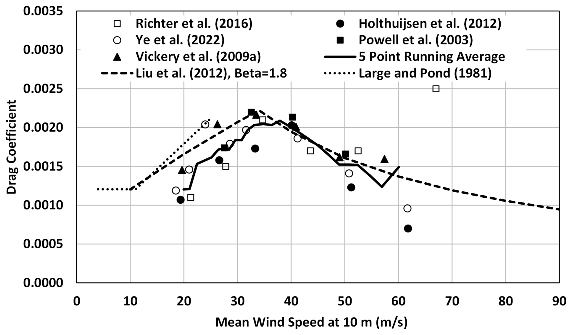
Figure 3 Variation of $C_{{\mathrm{d}}_{\mathrm{10}}}$ in tropical cyclones with mean wind speed from various studies obtained using the flux-profile method with GPS dropsondes plus the model given in Liu et al. (2012) and the Large and Pond (1981) model for wind speeds less than 25 m s⁻¹.

2.2 Gust factors

The characteristics of the near-surface turbulence within the marine boundary layer are needed to estimate peak wind speeds, turbulence intensities, velocity spectra, and so on. Unfortunately, there are very few detailed public domain measurements of turbulence in hurricanes over the ocean. High-resolution wind speed traces are not stored by the National Oceanic and Atmospheric Administration (NOAA)/National Climatic Data Center, whose data are limited to mean wind speeds (of various durations) and peak gust wind speeds (of various averaging times). Direct passages of the eyewall over an NOAA data buoy or a C-MAN station without failures of the anemometry are rare. To date, the highest 10 min mean wind speed at a NOAA station is 56.4 m s⁻¹, which was recorded at C-MAN station FYWF1 during Hurricane Andrew in 1992 at a height of 43.9 m.

He et al. (2021) report marine gust factors for mean wind speeds greater than 70 m s⁻¹. These data were recorded during Super Typhoon Hato using wind speed data recorded with an anemometer mounted on a 6.5 m mast, at an elevation of 60 m above sea level (m a.s.l.) on a small island in the South China Sea. The typhoon passed almost directly over the anemometer, which experienced high winds approaching first from the northwest and second from the southeast. The location of the anemometer on the island and the approximate range of wind directions associated with each passage of high winds are shown in Fig. 4.

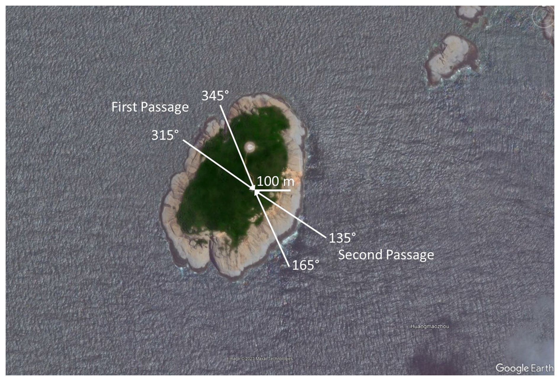
Figure 4 Image of the small island Huangmaohai (21.28° N, 113.96° E) in the South China Sea showing the location of the anemometer and the wind directions associated with the first and second passages of high winds. In the first passage, the anemometer is located about 200 m from the shoreline; for the second passage, the anemometer is about 150 m from the shoreline.

The anemometer recorded the maximum 3 s gust speed and the average 1 min wind speed every minute. He et al. (2020) used these data to compute the 3 s gust factor, defined as the maximum 3 s gust wind speed each minute divided by the 1 min mean wind speed in each interval. These data were averaged and binned into 10 m s⁻¹ bins, a summary of which is presented in Table 1.

Table 1 Gust factor data from He et al. (2020).

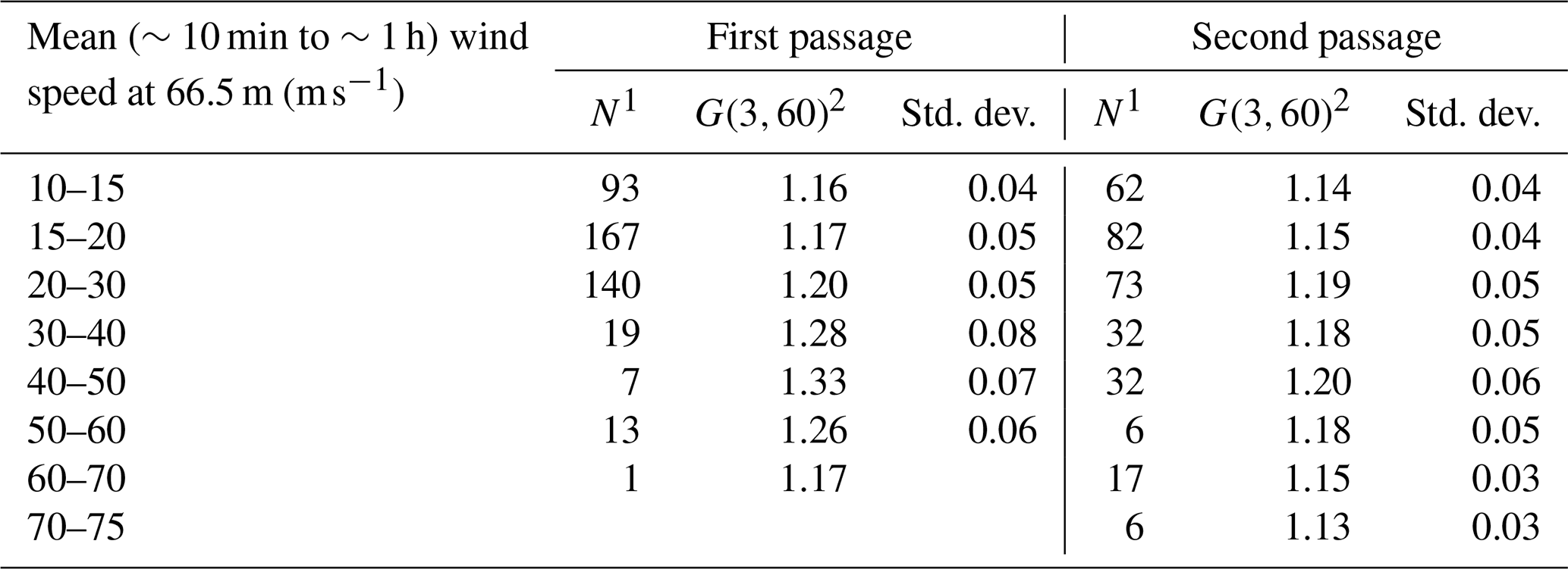
¹ N = Number of samples
² G(3,60) = 3 s peak gust wind speed recorded over a 60 s period divided by the mean wind speed averaged over 60 s.

The mean gust factors in each bin are plotted versus wind speed in Fig. 5. Because the wind speeds were averaged within each bin, the wind speeds represent a long term (e.g. 10 min to an hour); thus, the horizontal axis represents a mean wind speed rather than a 1 min wind speed – but a precise estimate of the effective averaging time is difficult to ascertain because the 1 min wind speeds and associated gust factors were sorted before being averaged. Also shown in Fig. 5 are the 1 min gust factors computed using the ESDU (1982, 1983) formulations for the gust factor coupled with the sea surface drag coefficient computed using three different assumptions. The sea surface drag coefficient models include that proposed by Large and Pond (1981) with maximum values of 0.0019 and 0.0023 and the model of Liu et al. (2012) using β=1.8 (fully developed). The maximum values of 0.0019 and 0.0023 are approximately the lower and upper bounds of the radius-dependent model used for $C_{{\mathrm{d}}_{\mathrm{10}}}$ discussed in Vickery et al. (2009a).

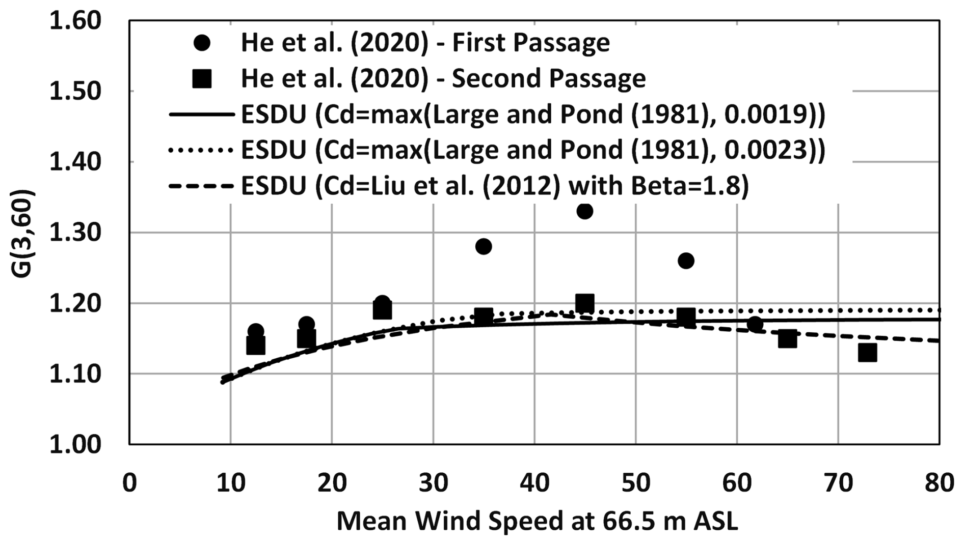
Figure 5 Modelled and measured (He et al., 2020) gust factors in high winds vs. mean wind speed in the South China Sea.

The modelled gust factors were computed assuming that the average wind speeds given in Table 1 are representative of a 10 min mean wind speed (i.e. maximum 10 min mean within an hour). The gust factors associated with the first and second passages yield similar trends, first increasing with wind speed, reaching a maximum, and then decreasing; however, the maximum values of the gust factors from the first and second passages are notably different: the gust factors from the first passage are much higher than those from the second passage for wind speeds between 30 and 50 m s⁻¹. It is not clear how the mean and gust wind speeds may have been influenced by the effects of the local terrain and topographic speed-ups induced by the island's terrain and topography. However, for each passage of strong winds, the influence of terrain, fetch, and wind speed-ups would not be expected to vary significantly because the range of directions associated with the strong winds is relatively narrow. The maximum mean wind speed of 72 m s⁻¹ at a height of 66.5 m a.s.l. (rightmost point in Fig. 5) corresponds to U₁₀ of about 61 m s⁻¹.

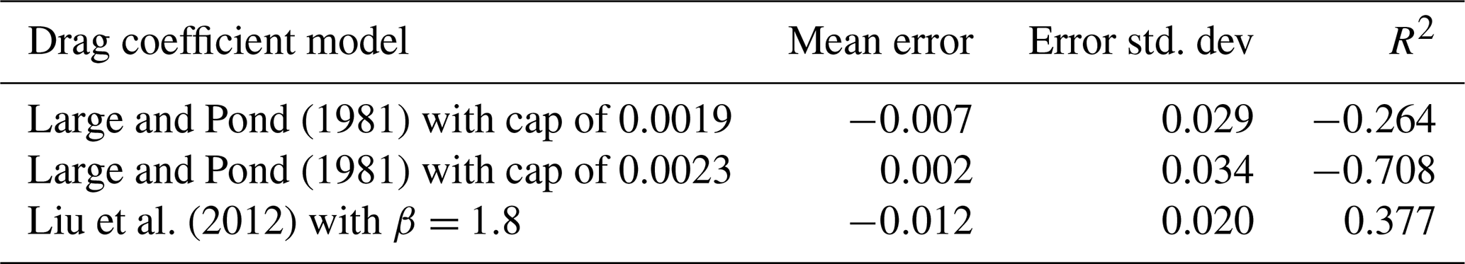
Statistics of the differences and the R² values associated with the comparison of the three gust factor models to the gust factor data from the second passage shown in Fig. 5 are summarized in Table 2. Not surprisingly, the model of Liu et al. (2012), as implemented here, produces the highest R², with the R² values from both Large and Pond (1981) models being negative.

Table 2 Quantitative comparisons of model and observed gust factors, G(3,60), at a height of 66.5 m. Observed gust factors from passage two as given in He et al. (2020).

Gust factor data from NOAA stations. All C-MAN data were collected from hurricanes affecting the Atlantic coast, and all buoy data were from Gulf of Mexico hurricanes. Both C-MANs and buoys report the maximum 5 s gust occurring in a 1 h period, the time at which the gust occurred, and a 10 min mean wind speed every 10 min. In the case of the buoy data, only data from the 10 m buoys were considered because wind data from buoys with anemometer heights of 3 and 5 m are thought to have been influenced by the local sea state because they drop into the wave troughs, where sheltering is expected.

A difficulty encountered when comparing the measured gust factors to modelled gust factors is associated with the lack of stationarity associated with hurricanes and the fact that there is only one measurement of the gust wind speed during an hour, whereas there are six 10 min means; hence, there are five other gust factors that may have (but not necessarily) all been lower than the one computed gust factor, which uses the largest gust wind speed within the hour.

Here, the measured 5 s gust factors are defined using two methods:

• (i)

  The largest 5 s gust recorded during a 1 h period divided by the 10 min mean wind speed recorded during the time at which the gust was measured.

• (ii)

  The largest 5 s gust recorded during a 1 h period divided by the 30 min mean wind speed computed using the average of the 10 min wind speed recorded during the time at which the gust was measured and the 10 min wind speeds occurring immediately before and after.

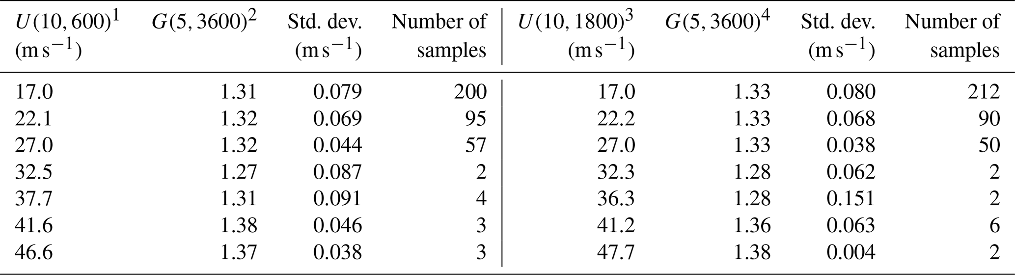
C-MAN gust factors. The anemometer heights for C-MANs DSLN7, FPSN7, and FWYF1 are 46.6, 44.2, and 43.9 m, respectively. All gust factor data from these three C-MANs were combined, with the analytic estimates of the gust factor computed using the average height of 44.9 m. Summaries of the gust factors from the C-MANs are presented in Table 3, where the number of samples and the mean and standard deviation of the gust factor are provided in each wind speed bin.

Table 3 Five-second gust factors from C-MAN stations DSLN7, FPSN7, and FWYF1. Measured gust factors computed using a 10 min mean wind speed (four columns on the left) and a 30 min mean wind speed (four columns on the right).

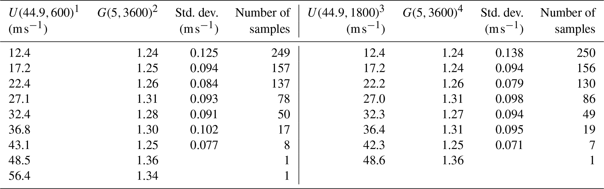
¹ U(44.9,600) = Mean wind speed at a height of 44.9 m averaged over a period of 600 s
² G(5,3600) = Max. 5 s peak gust recorded during a 3600 s period divided by the 3600 s mean wind speed
³ U(44.9,1800) = Mean wind speed at a height of 44.9 m averaged over a period of 1800 s
⁴ G(5,3600) = Max. 5 s peak gust recorded during a 3600 s period divided by the 3600 s mean wind speed.

The difference in the estimates of the gust factor computed using the 10 or 30 min mean wind speeds is negligible, with a maximum difference of less than 1 % and an average difference of less than 0.1 %, suggesting that the use of the 10 min mean wind speed within which the hourly peak gust wind speed was recorded is representative of G(5,3600).

Figure 6 presents gust factors computed from wind speed data obtained from the C-MAN stations during hurricanes along with the gust factors computed using the capped Large and Pond (1981) representation of the drag coefficient as well as the drag coefficient described in Liu et al. (2012). There are only ten 10 min mean wind speeds greater than 40 m s⁻¹ and only eight 30 min mean wind speeds greater than 40 m s⁻¹.

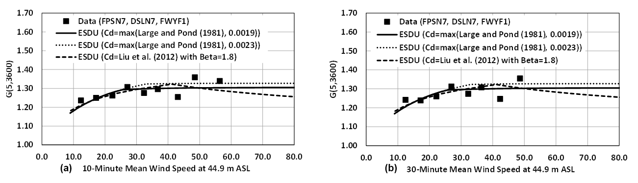
Figure 6 Modelled and measured gust factors at a height of 44.9 m. Measured gust factors from NOAA C-MAN stations based on a 10 min mean wind speed (a) and a 30 min mean wind speed (b).

Table 4 presents the error statistics (difference between the modelled and observed gust factors) for the three different modelled representations of the sea surface drag coefficient given in Fig. 6. The error statistics include the mean error, standard deviation of the error, and R². The summary statistics in Table 4 indicate that the gust factor at a height of 10 m is best modelled when the sea surface drag coefficient is modelled using the Large and Pond (1981) model with a cap of 0.0019.

Table 4 Quantitative comparisons of modelled and observed gust factors, G(5,3600), at a height of 44.9 m. Observed gust factors are from passage from C-MANs DSLN7, FPSN7, and FWYF1 and are computed using both 10 and 30 min mean wind speeds.

Buoy gust factors. Summaries of the gust factors from the buoy stations are presented in Table 5, where the number of samples and the mean and standard deviation of the gust factor are provided in each wind speed bin. As in the case of the gust factors from the C-MAN stations, the difference in the estimates of the gust factor computed using the 10 or 30 min mean wind speeds is small, with a maximum difference of about 2 % and an average difference of 0.2 %, again suggesting that the use of the 10 min mean wind speed within which the hourly peak gust wind speed was recorded is representative of G(5,3600). There are only six 10 min mean wind speeds greater that 40 m s⁻¹ and eight 30 min mean wind speeds greater than 40 m s⁻¹.

Table 5 Five-second gust factors from NOAA 10 m discus buoys. Measured gust factors computed using both 10 and 30 min mean wind speed.

¹ U(10,600) = Mean wind speed at a height of 10 m averaged over a period of 600 s
² G(5,3600) = Max. 5 s peak gust recorded during a 3600 s period divided by the 600 s mean wind speed
³ U(10,1800) = Mean wind speed at a height of 10 m averaged over a period of 1800 s
⁴ G(5,3600) = Max. 5 s peak gust recorded during a 3600 s period divided by the 1800 s mean wind speed.

Figure 7 presents gust factors computed from wind speed data obtained from the C-MAN stations during hurricanes along with the gust factors computed using the capped Large and Pond (1981) representation of the drag coefficient as well as the drag coefficient described in Liu et al. (2012).

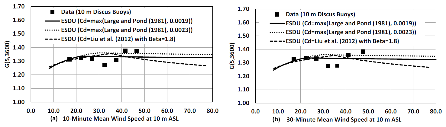
Figure 7 Modelled and measured gust factors at a height of 10.0 m. Measured gust factors from 10 m NOAA discus buoys, based on a 10 min mean wind speed (a) and a 30 min mean wind speed (b).

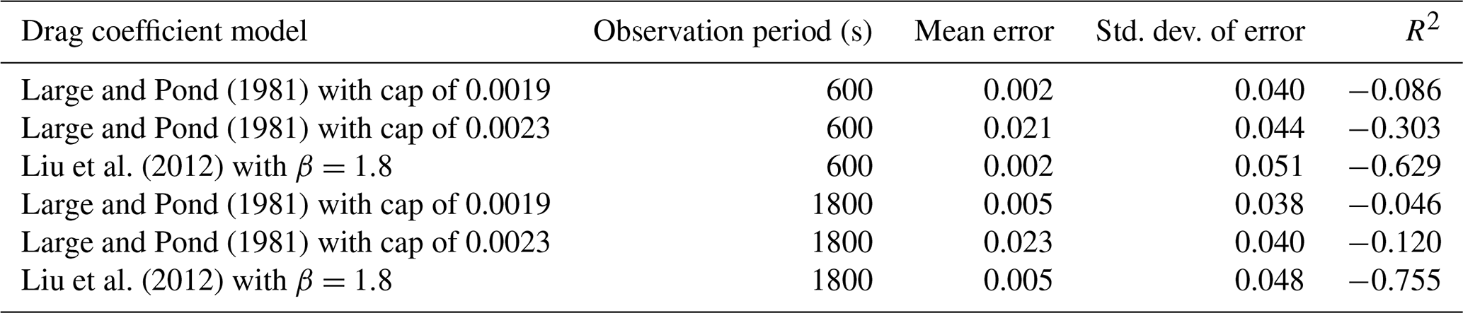
Summary statistics are provided in Table 6, where it is seen that $C_{{\mathrm{d}}_{\mathrm{10}}}$ modelled using the Liu et al. (2012) model performs worst and the Large and Pond (1981) formulation with a cap of 0.0019 performs best but still yields a negative R². The poor performance of the models is due to the observed apparent outlier gust factors for U₁₀ between 30 and 40 m s⁻¹.

Table 6 Quantitative comparisons of model and observed gust factors, G(5,3600), at a height of 10 m. Observed gust factors from 10 m discus buoys computed using both 10 and 30 min mean wind speeds.

2.3 Drag coefficient summary

The review of the literature pertaining to the behaviour of sea surface drag coefficients as a function of wind speed in hurricanes, coupled with the analysis of gust factors over the ocean in hurricanes, leads to somewhat ambiguous conclusions.

There is no direct method to measure the sea surface drag coefficient; therefore, indirect methods are used. Currently, there is no consensus on which of the methods discussed herein yields the most reliable solutions, and there is still significant uncertainty about the behaviour of $C_{{\mathrm{d}}_{\mathrm{10}}}$ at very high (ultimate design) wind speeds, which largely occur near the eyewall of hurricanes.

The gust factor analysis using NOAA data suggests that the drag coefficient does not reach a maximum for U₁₀ around 33 m s⁻¹ as suggested in Powell et al. (2003) and, by extension, suggests that $C_{{\mathrm{d}}_{\mathrm{10}}}$ is perhaps limited by the action of sea spray, but this decrease does not occur until U₁₀ reaches approximately 50 m s⁻¹. The analysis of gust factors derived from the NOAA platforms suggests that the model for the sea surface drag coefficient capped at 0.0019 provides the best description of $C_{{\mathrm{d}}_{\mathrm{10}}}$. The gust factor data described in He et al. (2021) suggest that $C_{{\mathrm{d}}_{\mathrm{10}}}$ decreases for U₁₀ greater than about 50 m s⁻¹.

The suggestion of Smith and Montgomery (2014) that the flux-profile method may not be valid near the eyewall implies that the use of the flux-profile approach leads to an underestimate of the true value of $C_{{\mathrm{d}}_{\mathrm{10}}}$. As noted in the preceding discussion, the Liu et al. (2012) model with β=1.8 appears to be the best model for describing the drag coefficient computed using the flux method. The Liu et al. (2012) model with β=1.8, coupled with the ESDU (1983) model for turbulence intensity, provides the best model for the gust factors on the island of Huangmaoxhou, whereas the use of the Large and Pond (1981) model with a cap of 0.0019 provides the best model for gust factors computed from C-MANs and buoys. Owing to the uncertainty associated with the use of the log-law to estimate $C_{{\mathrm{d}}_{\mathrm{10}}}$ near the core of a hurricane, we conservatively recommend the use of the capped Large and Pond (1981) model, which may overestimate U₁₅₀ but yields reasonable estimates of gust factors.

The relationship between the maximum 1 min wind speeds at the Saffir–Simpson hurricane category break points and wind speeds associated with other average times at heights of 10 and 150 m a.s.l. is given in Table 7. IEC 61400-1 (IEC TC88-MT1 2019) defines the reference wind speed as a 10 min average wind speed with a return period of 50 years at turbine hub height. The reference wind speed values for Class 1A and Typhoon Class are provided in Table 1 of IEC 61400-1 as 50 and 57 m s⁻¹ (111.9 and 127.5 mph), respectively.

Table 7 Wind speeds in m s⁻¹ (mph) at the break points between hurricane categories. Wind speeds are given at heights of 10 and 150 m for averaging times of 1 h, 10 min, 1 min, and 3 s. Wind speeds are computed using a sea surface drag coefficient of 0.0019 and the ESDU (1982) model for the mean boundary layer.

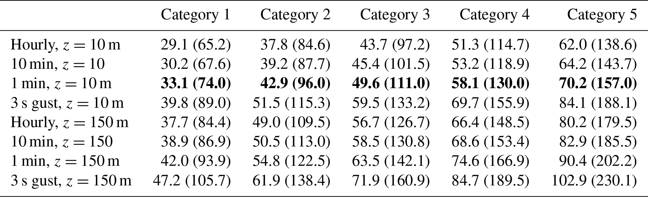
According to Table 7 and assuming a hub height of 150 m, the Class 1A reference wind speed is associated with the lower limit of a Category 2 hurricane, and the Typhoon Class reference wind speed is associated with just under the lower limit of a Category 3 hurricane. The IEC 3 s extreme gust criteria, which are 70 m s⁻¹ for Class 1A turbines and 80 m s⁻¹ for Typhoon Class turbines, are associated with a strong Category 2 and a moderate Category 3 hurricane, respectively.

Based largely on the gust factor comparisons and the drag coefficient data presented in Fig. 3, we suggest that, for the lower 100 to 200 m, the hurricane boundary layer be modelled using a mean profile described using the log-law as given in Eq. (1) and a drag coefficient model that uses the Large and Pond (1981) model with an upper limit of 0.0019. This model for $C_{{\mathrm{d}}_{\mathrm{10}}}$ results in a relatively low $C_{{\mathrm{d}}_{\mathrm{10}}}$ at high wind speeds but does not yield a reduction in $C_{{\mathrm{d}}_{\mathrm{10}}}$. The model is possibly conservative; however, until consensus is reached on the behaviour of $C_{{\mathrm{d}}_{\mathrm{10}}}$ at high wind speeds in hurricanes, we believe that this approach is prudent. The turbulence characteristics of the wind are well modelled using the ESDU (1982, 1983) models for atmospheric turbulence.

3 Hurricane hazard modelling

The key components of the hurricane hazard model are (i) probabilistic models describing the occurrence rates, storm tracks, and intensities (Vickery et al., 2009b) and (ii) the hurricane wind field model (Vickery et al., 2009a). Section 3.1 provides an overview of the track modelling approach and presents validation examples in the Gulf of Mexico region encompassing the offshore wind energy area. For full details on the development and validation of the wind field model, including modelling the variation in wind speed with height, see Vickery et al. (2009a).

3.1 Hurricane track and intensity modelling

The probabilistic portion of the hurricane hazard model is described in detail in Vickery et al. (2000b, 2009b). The key features of the storm track model are the coupling of the modelling of the central pressure with sea surface temperature (SST) and the ability to model curved tracks that can make multiple landfalls. The entire track of a storm is modelled, from the time of storm initiation over the water until the storm dissipates. The starting times (hour, day, and month) and locations of the storms are taken directly from HURDAT2 (Landsea and Franklin, 2013). Using the actual starting times and locations ensures that any climatological preference for storms to initiate in different parts of the Atlantic Basin at different times of the year is maintained. Limitations of the model arise from dependency on the observational record, the completeness of which varies prior to the onset of aircraft reconnaissance and satellite capabilities.

The coupling of the central pressure modelling to sea surface temperature ensures that intense storms (such as Category 5 storms) cannot occur in regions in which they physically could not exist (such as at extreme northern latitudes). As shown in Vickery et al. (2000b, 2009b), the approach reproduces the variation in the central pressure characteristics along the United States coastline. In the hurricane hazard model, the storm's intensity is modelled as a function of the sea surface temperature and wind shear until the storm makes landfall. At the time of landfall, the filling models described in Vickery (2005) are used to exponentially decay the intensity of the storm over land. Over land, following the approach outlined in Vickery et al. (2009b), the storm size is modelled as a function of central pressure and latitude. If the storm exits land into the water, the storm intensity is again modelled as a function of sea surface temperature and wind shear, allowing the storm to possibly reintensify and make landfall again elsewhere.

The validity of the modelling approach for storms near the coastal United States is shown through comparisons of the statistics of historical and modelled key hurricane parameters along the North American coast. Comparisons of occurrence rate, heading, translation speed, distance of closest approach, and so on, are given in Vickery et al. (2009b). These comparisons are made using the statistics derived from historical and modelled storms that pass within 250 kilometres (km) of a coastal milepost location. The comparisons are also given for mileposts spaced 50 nautical miles apart along the entire United States Gulf and Atlantic coastlines. In all comparison figures in Vickery et al. (2009b), the 90 % confidence bounds are also plotted and shown to encompass the historical data, indicating with 90 % confidence that the historical and modelled data are from equivalent statistical distributions. Results of additional statistical testing using the chi-square, Kolmogorov–Smirnov, and James and Mason tests of equivalent distributions are also provided, indicating that the confidence in equivalent distributions of some track modelling parameters may be as high as 95 %. Validation examples are also presented later in this section.

3.2 Hurricane track and intensity validation

The HURDAT2 database is used to validate the model away from the U.S. coastline. HURDAT2 contains position data (latitudes and longitudes), central pressures, and estimates of the maximum wind speed (maximum 1 min average wind speed at a height of 10 m) given in increments of 2.57 m s⁻¹. Prior to the satellite era (∼1970), information on central pressure was limited to near-shore estimates obtained by reconnaissance aircraft. These limited aircraft data are available starting in the mid-1940s. Prior to the aircraft era, estimates of central pressure were derived from ship reports and other ground sources. The HURDAT2 data are archived at 6 h increments. Furthermore, central pressures other than those at the start and end of each 6 h segment are not recorded. Therefore, it is unlikely that one of these 6 h positions contains the minimum central pressure experienced over the life of a storm.

In addition to the information obtained from the HURDAT2 dataset, the model is validated/calibrated using a separate dataset that provides details on landfall pressures (Blake et al., 2011). Both the landfall dataset and the HURDAT2 dataset are continually being updated through the ongoing HURDAT2 reanalysis project (http://www.aoml.noaa.gov/hrd/data_sub/re_anal.html, last access: 1 October 2020). The HURDAT2 dataset used here includes all revisions to historical storm data through the June 2019 HURDAT2 update.

Figures 8 and 9 present example comparisons of the modelled and historical cumulative distribution functions (CDFs) of storm heading (i.e. the direction a storm is travelling) and storm translation speed (i.e. the speed at which a storm is travelling) in the Gulf of Mexico. In addition to the CDFs, Figs. 8 and 9 also include a simplified coastline of the western Gulf of Mexico from Mexico to Louisiana, as shown by the blue line. Each CDF was developed using information on all historical tropical cyclones passing within 250 km of a specified latitude–longitude pair. These validation circles are centred on a 2° grid, with the results presented here encompassing the western Gulf of Mexico from 22 to 32° N latitude and 90 to 98° W longitude.

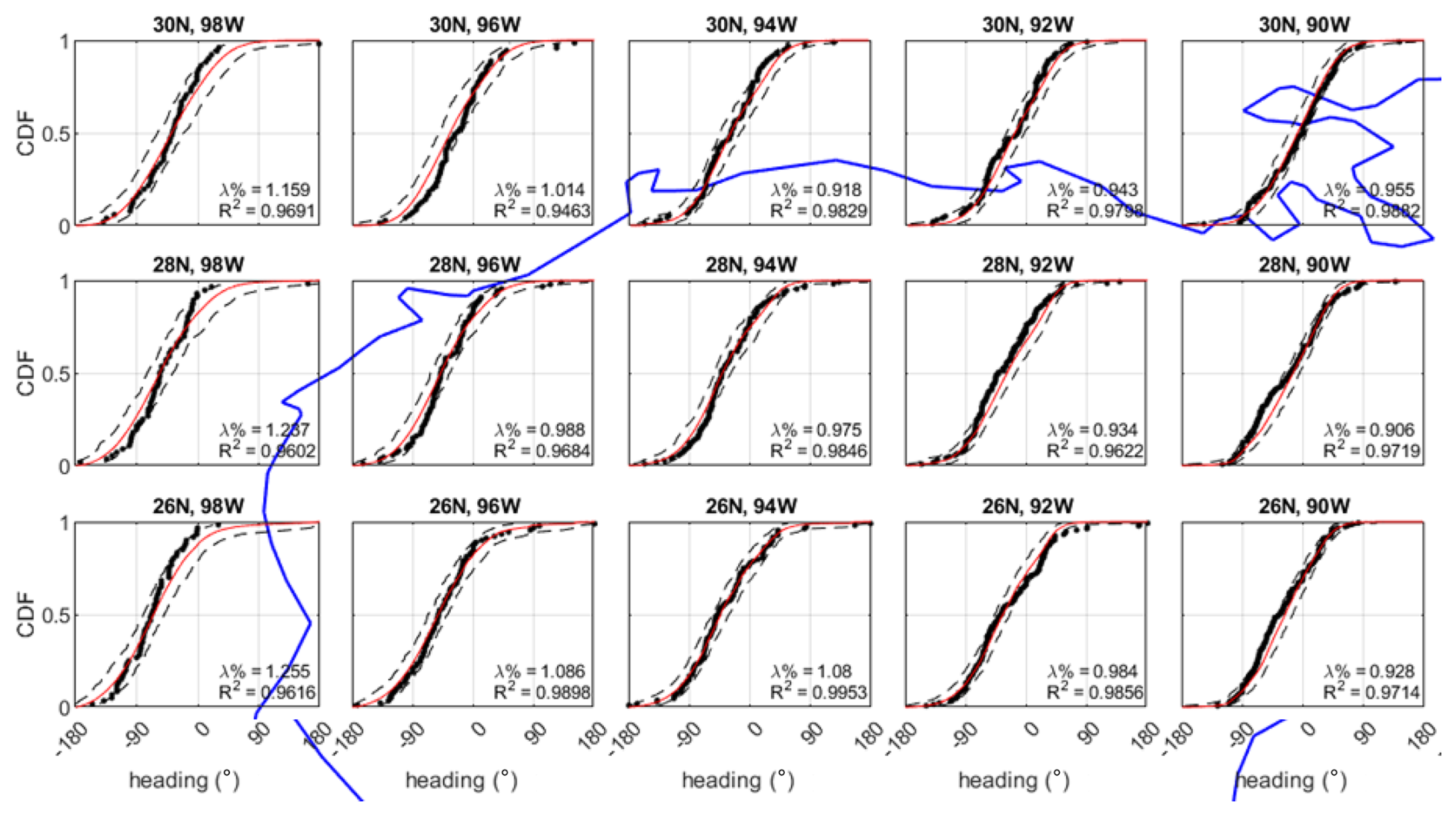
Figure 8 Comparison of the modelled and observed cumulative distribution functions (CDFs) for storm heading. Values are the heading of the storm at the time it was nearest to the centre of a 250 km radius circle centred on the point indicated by the title of each graph. Observations are shown by black dots, modelled values are shown by the red line, and 95 % confidence bounds are shown by the black dashed lines. The western Gulf of Mexico coastline is shown by the blue line for orientation purposes.

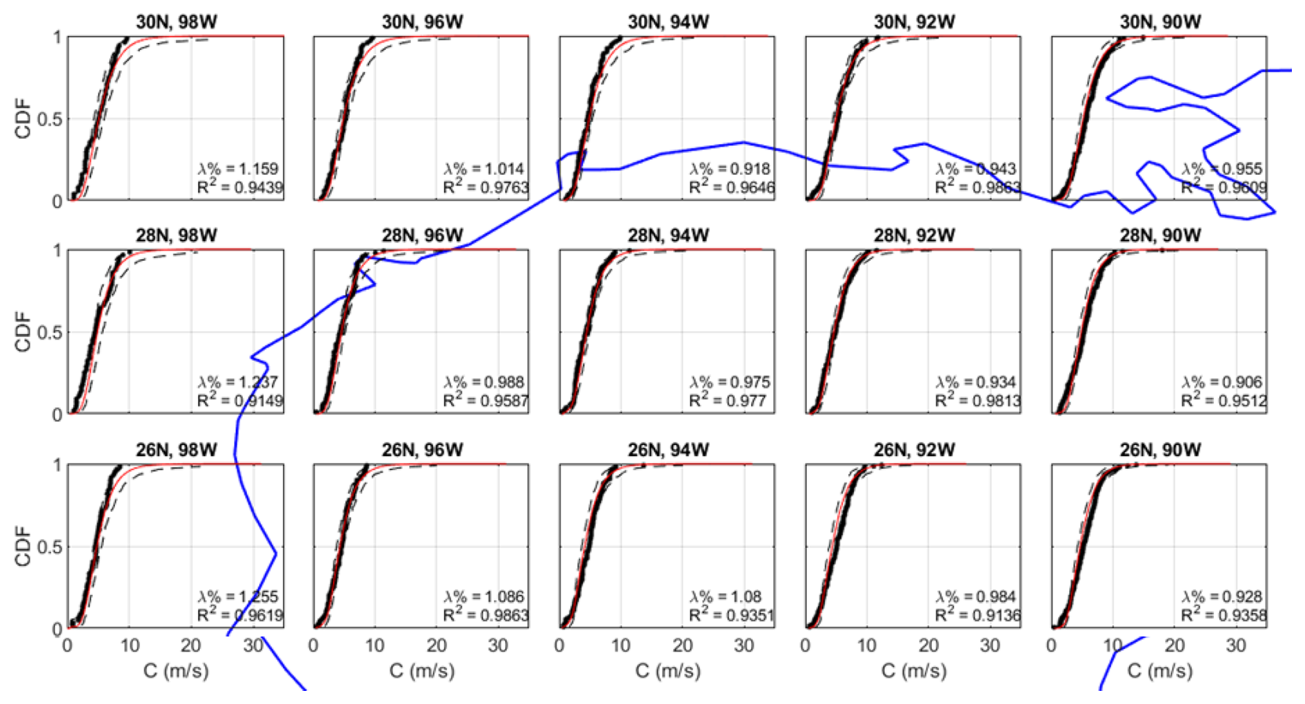
Figure 9 Comparison of the modelled and observed cumulative distribution function (CDF) for storm translation speed. Values are the storm translation speed at the time it was nearest to the centre of a 250 km radius circle centred on the point indicated by the title of each graph. Observations are shown by black dots, modelled values are shown by the red line, and 95 % confidence bounds are shown by the black dashed lines. The western Gulf of Mexico coastline is shown by the blue line for orientation purposes.

Figure 10 presents example comparisons of modelled and observed central pressures plotted versus the return period. For orientation purposes, a simplified coastline of the western Gulf of Mexico from Mexico to Louisiana is also shown by the blue line in Fig. 10. The observed central pressures plotted versus the return period were computed assuming that the Np pressure data points obtained from a total of N tropical cyclones that pass through the circle are representative of the full population of N storms. With this assumption, the CDF for the conditional distribution for storm central pressure is computed, where each pressure has a probability of $\mathrm{1}/(Np+\mathrm{1})$. The return period associated with a given central pressure is obtained from

$$\begin{array}{}\text{(9)}& P_t(p_{\mathrm{c}}<P_{\mathrm{c}})=\mathrm{1}-\sum _{x=\mathrm{0}}^{\mathrm{\infty }}{P}_t(p_{\mathrm{c}}>P_{\mathrm{c}}\mathrm{|}x)p_t\left(x\right),\end{array}$$

where P_t(p_c>P_c|x) is the probability that velocity v is less than V given that x storms occur and p_t(x) is the probability of x storms occurring during time period t. From Eq. (9), with p_t(x) defined as Poisson and t defined as 1 year, the annual probability of exceeding a given wind speed is

$$\begin{array}{}\text{(10)}& P_{\mathrm{a}}(p_{\mathrm{c}}<P_{\mathrm{c}})=\mathrm{1}-\exp [-\mathit{\lambda }P(p_{\mathrm{c}}<P_{\mathrm{c}}\left)\right],\end{array}$$

where λ is the annual occurrence rate, defined as $N/N_{\mathrm{Y}}$, with N_Y being the number of years in the historical record, here equal to 120 years (1900 through 2019).

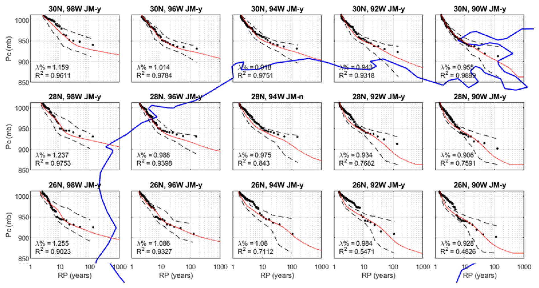
Figure 10 Comparison of modelled and observed central pressure plotted vs. the return period. Values correspond to the minimum central pressure given in millibars (mbar) while the storm is within a 250 km radius circle centred on the point indicated by the title of each graph. Observations are shown by black dots, modelled values are shown by the red line, and 95 % confidence bounds are shown by the black dashed lines. The western Gulf of Mexico coastline is shown by the blue line for orientation purposes. Note: JM-y indicates that the modelled central pressures pass the 95 % confidence test using the James–Mason test.

The model estimates of central pressure versus the return period for a given location are computed using Eq. (10), where λ is the annual occurrence rate of simulated storms affecting the location of interest (e.g. the number of simulated storms within 250 km of a location divided by the number of simulated years). The probability distribution for central pressure is obtained by rank ordering the simulated central pressures. The comparisons of modelled and observed central pressures given in Fig. 10 use the minimum value of the central pressures while a storm (modelled or historical) is within 250 km of the indicated point.

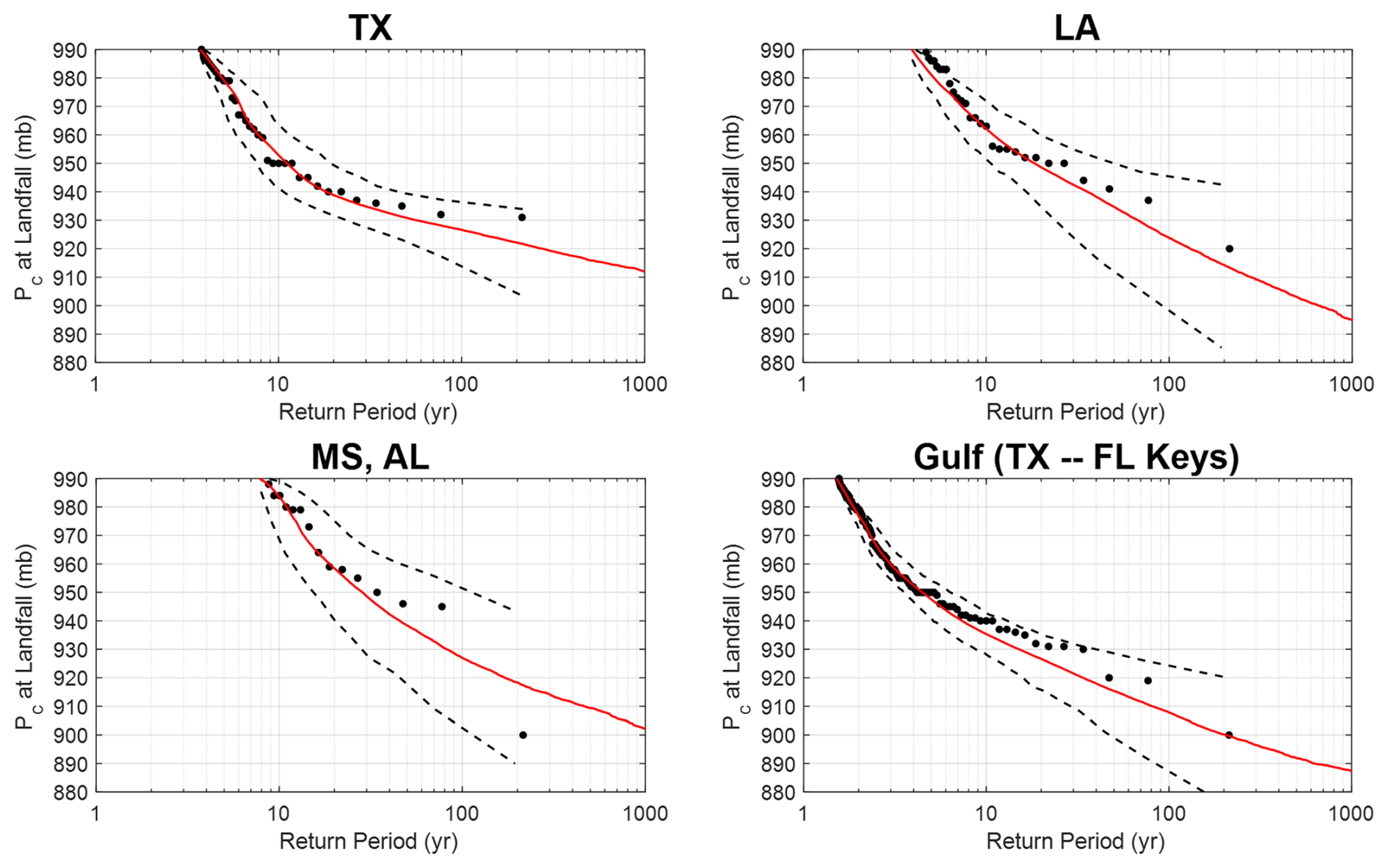
Figure 11 Comparison of modelled and observed central pressures at landfall along the Texas, Louisiana, Mississippi, and Alabama coastlines and the Gulf of Mexico coastline (Texas to Florida Keys). Observations are shown by black dots, modelled values are shown by the red line, and 95 % confidence bounds are shown by the black dashed lines.

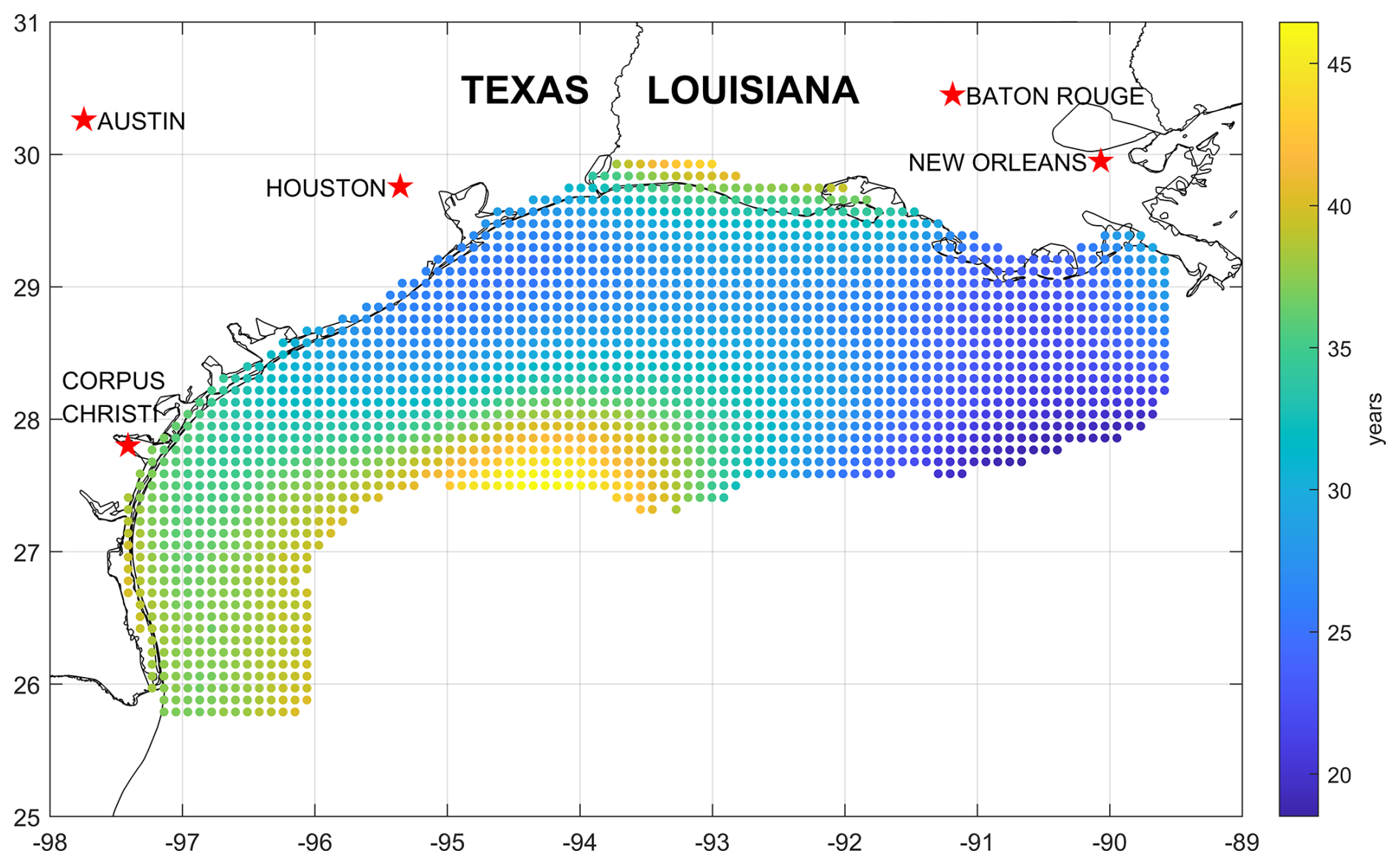
Figure 12 Return period (years) associated with the IEC Class 1A limit-state reference wind speed of 111.9 mph (50 m s⁻¹) obtained from a 500 000-year hurricane simulation.

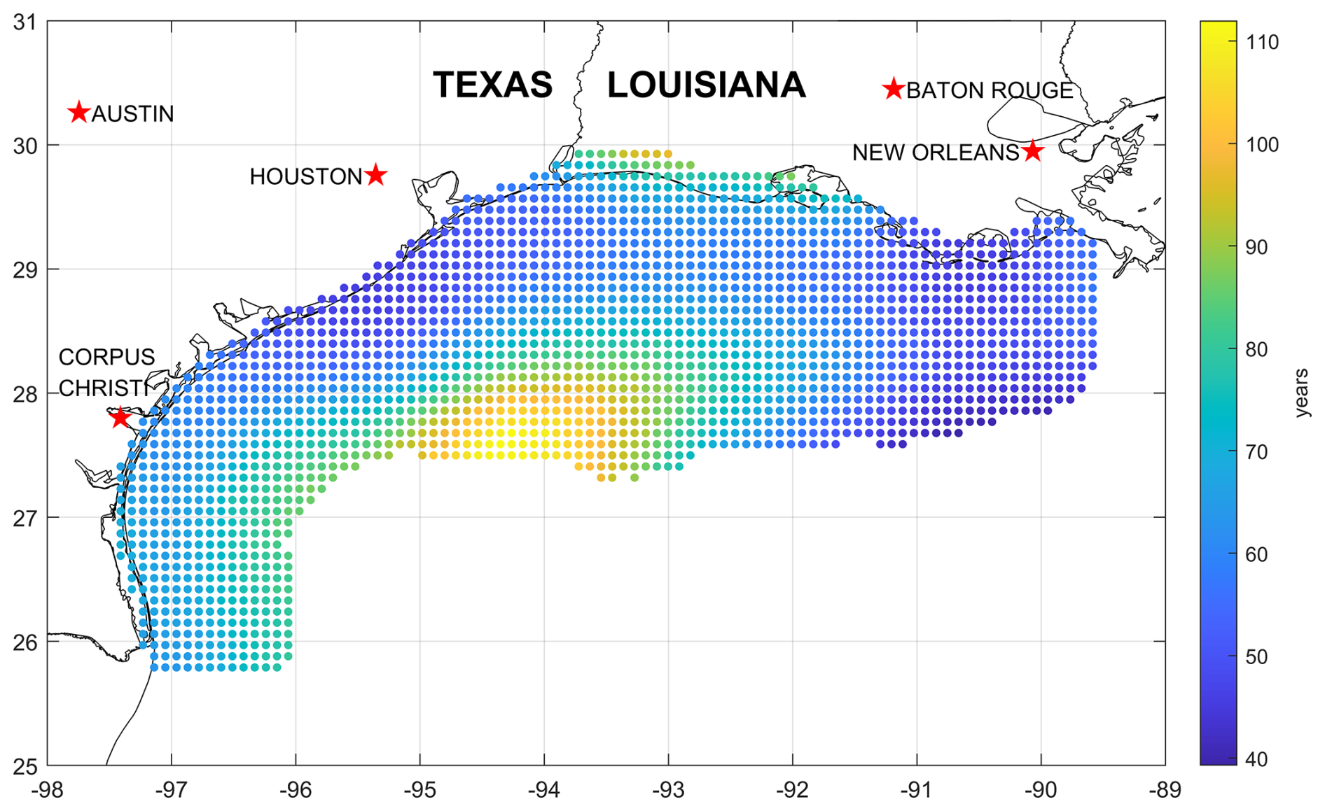
Figure 13 Return period (years) associated with the IEC Typhoon Class limit-state reference wind speed of 127.5 mph (57 m s⁻¹) obtained from a 500 000-year hurricane simulation.

In addition to the mean model estimates of pressure vs. the return period in each of the plots given in Fig. 10, these figures also present the 2.5th and 97.5th percentile (95 % confidence range) values of central pressures derived by sampling Np different values of central pressure from the simulated storm set and computing the CDF and then the pressure return period (RP) curve using the model value of λ. This process is repeated 900 times, yielding 900 different RP curves based on sampling Np pressures randomly from the simulated storm set. The 900 different RP curves are then used to define the 95 % confidence range for the mean pressure RP curves. In our testing, we include only tropical cyclones with central pressures less than 980 mbar, which is the threshold for a Category 1 event on the Saffir–Simpson hurricane scale. The pc-RP curves yield comparisons that include the combined effects of the modelling of central pressures and the frequency of occurrence of the storms.

Figure 11 presents a comparison of estimates of the landfall pressure as a function of the return period. The historical data were obtained from HURDAT2 and Blake et al. (2011). The Blake et al. (2011) data include central pressure information from all hurricanes that have made landfall in the United States. HURDAT2 was used to obtain information on the central pressures for all landfalling tropical storms. As in the case of the comparisons of central pressure plotted vs. the return period developed from the data passing within 250 km of a given point, each of the plots given in Fig. 11 also presents the 2.5th and 97.5th percentile (95 % confidence range) values of central pressures derived by resampling. The historical data fall well within the range defined by the 95 % confidence bounds.

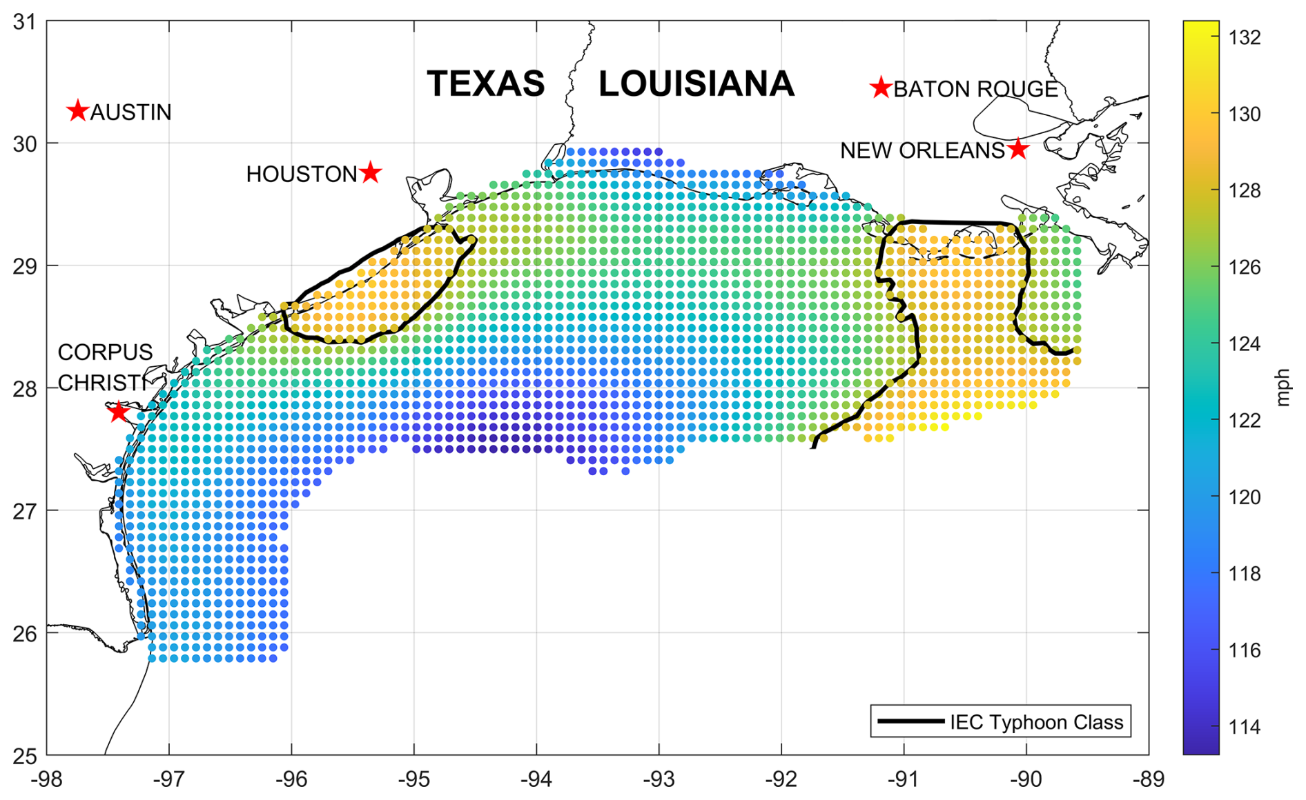
Figure 14 The 10 min sustained wind speed (mph) at 150 m with a return period of 50 years obtained from a 500 000-year hurricane simulation. Note: No isocline for the Class 1A limit state appears because all simulated values of the 50-year wind speed are greater than the Class 1A reference wind speed (111.9 mph, 50 m s⁻¹).

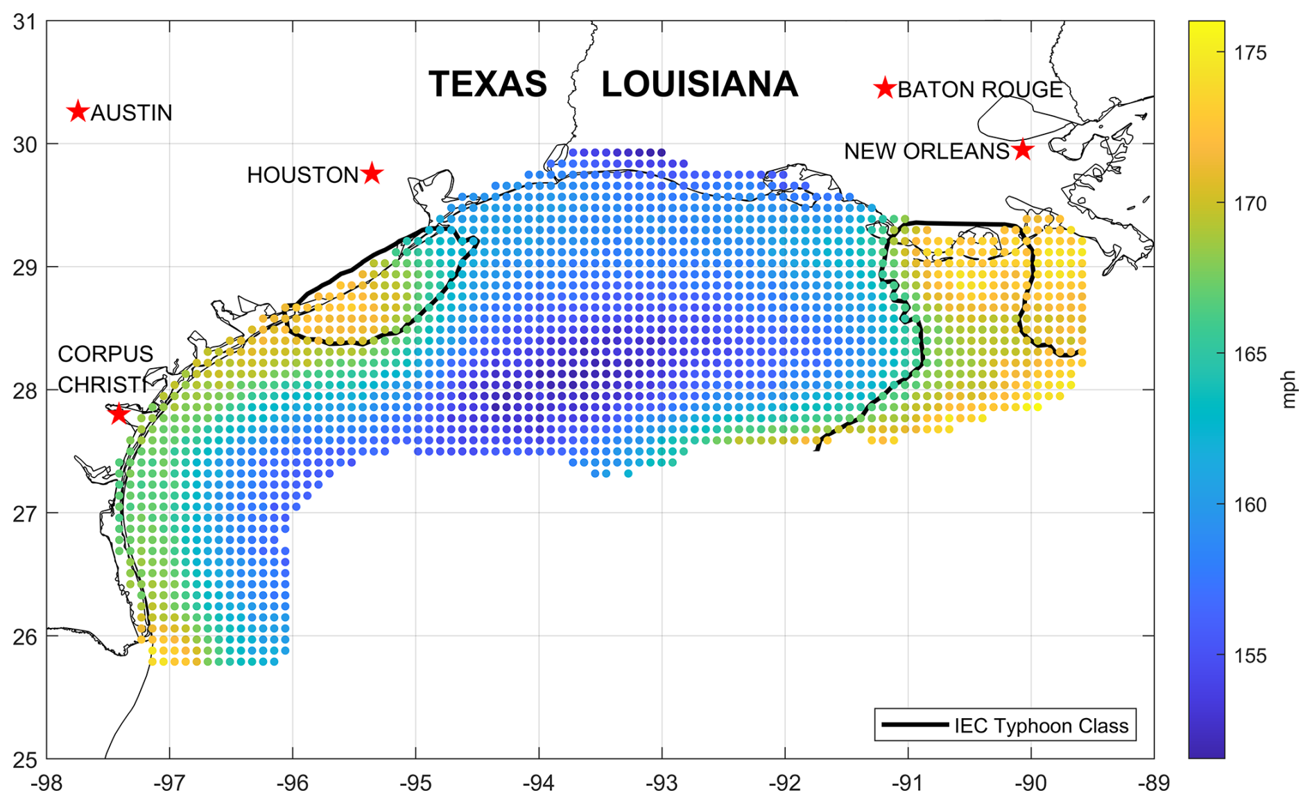
Figure 15 The 10 min sustained wind speed (mph) at 150 m with a return period of 500 years obtained from a 500 000-year hurricane simulation. Note: No isocline for the Class 1A limit state appears because all simulated values of the 50-year wind speed are greater than the Class 1A reference wind speed (111.9 mph, 50 m s⁻¹).

3.3 Geospatial risk assessment

Upon completion of a 500 000-year simulation, the wind speed data are rank ordered and then used to define the wind speed probability distribution, P(v>V), conditional on a storm having passed within 250 km of the site. A simulation period of 500 000 years was employed to provide a sufficiently long period of record such that wind speed probability distributions, and the corresponding confidence intervals, for return periods up to 10 000 years could be estimated. The probability that the tropical cyclone wind speed (independent of direction) is exceeded during time period t is

$$\begin{array}{}\text{(11)}& P_t(v>V)=\mathrm{1}-\sum _{x=\mathrm{0}}^{\mathrm{\infty }}P(v<V\mathrm{|}x)p_t\left(x\right),\end{array}$$

where P(v<V|x) is the probability that velocity v is less than V given that x storms occur and p_t(x) is the probability of x storms occurring during time period t. P(v<V|x) is obtained by interpolating from the rank-ordered wind speed data. From Eq. (12), with p_t(x) defined as Poisson and t defined as 1 year, the annual probability of exceeding a given wind speed is

$$\begin{array}{}\text{(12)}& P_{\mathrm{a}}(v>V)=\mathrm{1}-\exp [-\mathit{\lambda }P(v>V\left)\right],\end{array}$$

where λ represents the average annual number of storms approaching within 250 km of the site (i.e. the annual occurrence rate).

IEC 61400-1 (IEC TC88-MT1 2019) defines the reference wind speed as a 10 min average wind speed with a return period of 50 years at turbine hub height. The reference wind speed values for Class 1A and Typhoon Class are provided in Table 1 of IEC 61400-1 as 111.9 and 127.5 mph (50 and 57 m s⁻¹), respectively.

Here, using Eq. (12), we estimated return periods associated with the IEC Class 1A and Typhoon Class limit-state hurricanes on a nominal 10 km by 10 km grid covering the Gulf of Mexico offshore resource area, as shown in Figs. 12 and 13, respectively. Hub height was assumed to be 150 m, which is typical for the 15 MW class turbines that may be deployed and is the hub height of the National Renewable Energy Laboratory (NREL) 15 MW reference turbine (Gaertner et al., 2020). The wind speed at hub height is needed for comparison with the IEC 61400 design standards. The return period associated with the Class 1A limit state ranges from approximately 20 to 45 years, whereas the return period associated with the Typhoon Class limit state ranges from approximately 40 to 110 years.

The 10 min average wind speed for return periods of 50 and 500 years at turbine hub height obtained from the 500 000-year simulation are also presented on the same grid in Figs. 14 and 15, respectively. The figure indicates that the 50-year reference wind speed across the Gulf of Mexico offshore resource area ranges from approximately 114 to 132 mph (51 to 59 m s⁻¹) and the 500-year values range from approximately 151 to 176 mph (68 to 79 m s⁻¹). Isoclines are also plotted corresponding to the IEC Typhoon Class design limit state. Note that no isocline for the Class 1A limit state appears because all 50-year wind speed values obtained from the simulation are greater than the Class 1A reference wind speed (111.9 mph, 50 m s⁻¹ for a 50-year return period at 150 m).

4 Summary

A challenge in relating a given hurricane event to the IEC design criteria stems from inconsistent hurricane wind speed terminology between the Saffir–Simpson hurricane scale, used by the National Hurricane Center to estimate the intensity of hurricanes, and IEC design criteria used for the design of turbines. Using the latest research on turbulence characteristics of the hurricane boundary layer, definitions of the Saffir–Simpson wind speed scale are provided in Sect. 2.3 for four averaging times (i.e. 3 s, 1 min, 10 min, and 1 h) and two heights (i.e. 10 and 150 m). In the same section, definitions of the Class 1A and Typhoon Class limit states are provided in terms of an equivalent Saffir–Simpson category.

For the boundary layer model used, we compared the relationship between the maximum 1 min wind speeds at the Saffir–Simpson hurricane category break points at 10 m height and wind speeds associated with 3 s averaging times used by IEC wind turbine design standards at 150 m height. The 70 m s⁻¹ 3 s gust for Class 1A turbines was found to be associated with a strong Category 2 hurricane, and the 80 m s⁻¹ 3 s gust for Typhoon Class turbines was found to be associated with a moderate Category 3 hurricane.

Using the hurricane hazard model outlined herein, the wind hazard for the Gulf of Mexico offshore wind energy area was defined on a grid with a nominal resolution of 10 km. Results of the geospatial risk assessment are provided in Sect. 3.3. The IEC prescribes the reference wind speeds associated with Class 1A and Typhoon Class limit states to be 50 years, though the return periods associated with the Class 1A limit state were found to range from approximately 20 to 45 years, while the return period associated with the Typhoon Class limit state ranges from approximately 40 to 110 years. This indicates that the Class 1A limit state may be nonconservative for the entire Gulf of Mexico offshore wind energy area, while the Typhoon Class limit state may be adequate for the design of turbines in some regions of the Gulf of Mexico offshore wind energy area. A map of the 10 min mean wind speeds at 150 m height associated with a return period of 50 years is also provided. The 50-year value was found to range from approximately 114 to 132 mph (51 to 59 m s⁻¹).