A robust active power control algorithm to maximize wind farm power tracking margins in waked conditions

We present an active power control (APC) algorithm for wind farms that operates wind turbines to maximize their power availability in order to robustly track a reference power signal in the presence of turbulent wind lulls. The operational setpoints of the wind turbines are optimized using an engineering flow model by combining induction control with wake steering. The latter has the goal of deflecting low-momentum wakes and increasing power margins. The algorithm also features a proportional–integral closed loop inspired by the literature to correct potential errors deriving from the offline computation of the setpoints.

First, we demonstrate the new approach in steady-state conditions, showing how the availability of power is increased by mitigating wake interactions. We observe that our proposed method is particularly effective in conditions of strong wake impingement, occurring in scenarios of high power demand. Next, considering two wind farm layouts, we compare the performance of the algorithm to three state-of-the-art reference APC formulations in unsteady scenarios using large-eddy simulations coupled with the actuator line method (LES-ALM). We show that the occurrence and treatment of local temporary instances of power unavailability (saturations) dramatically affect power tracking accuracy. The proposed method yields superior power tracking due to the increased power margins that limit the occurrence of saturation events. Additionally, we show that this performance is achieved with reduced structural fatigue.

1 Introduction

As renewable energy sources occupy a larger portion of the electricity mix, they must become also capable of providing extra functionalities to the grid, beyond the pure generation of power (Aho et al., 2012; Ela et al., 2014). Among these extra operating modes, active power control (APC) is a strategy where generating assets are intentionally operated below their maximum output to satisfy operational constraints imposed by the transmission system operator (TSO).

In the context of wind energy, the APC problem is particularly challenging due to the dynamics of mesoscale weather phenomena, the two-way interaction of the atmospheric boundary layer with a wind farm, the complex development of the flow within the plant, and its local interaction with the aeroelastic behavior of wind turbines. The maximum available power that can be generated by a wind farm at any given time is strongly influenced by site and local turbine-specific ambient conditions, which change over time in uncertain and difficult-to-predict ways (van Kuik et al., 2016). As a result, sudden drops in wind speed or inaccuracies in forecasts can result in inadequate power reserves, making it difficult to follow a given reference signal (Fleming et al., 2016).

In a wind farm, the situation is further complicated by the presence of low-momentum turbulent wakes, which lead to power losses and contribute to fatigue loading on frequently waked turbines (Vermeer et al., 2003; Lee et al., 2013; Guilloré et al., 2024). A variety of approaches have been suggested to reduce the impact of wake effects, such as induction, yaw control, and mixing (Meyers et al., 2022). Yaw control, in particular, involves “steering” the wakes away from downstream turbines. Its effectiveness in boosting power has been demonstrated in numerical simulations (Jiménez et al., 2010; Fleming et al., 2014; Vollmer et al., 2016), wind tunnel experiments (Medici and Alfredsson, 2006; Campagnolo et al., 2016; Schottler et al., 2017), and real-world field trials (Fleming et al., 2019; Doekemeijer et al., 2021). In recent years, machine learning techniques have been increasingly integrated into wake mitigation strategies, further enhancing their effectiveness (Meyers et al., 2022; Ally et al., 2025).

Different APC approaches have been described and tested in the literature. The most straightforward method uses an open-loop strategy, where each turbine is given a predefined power share setpoint (Fleming et al., 2016). However, unsurprisingly, the absence of feedback reduces the power tracking accuracy, particularly under strong wake impingement conditions. Additionally, uniformly distributing power among turbines may result in suboptimal performance, as the local power availability varies among different turbines due to wake effects.

Various authors have used model predictive control (MPC) for APC (Shapiro et al., 2017; Boersma et al., 2018). The main drawback of such methods lies in the need for a dynamic farm flow model, which increases complexity and computational cost. While such methods undoubtedly have their own merits, here we are interested in solutions that are closer to practical applicability and a more rapid uptake from industry.

Classical PID (proportional–integral–derivative) controllers are widely used in an extremely broad range of different industrial applications. As a result, they have also been widely studied for wind farm APC (van Wingerden et al., 2017). While these methods lack the sophistication of MPC, they do not require a dynamic wind farm flow model and can offer quick response times with straightforward implementations.

The APC PI (proportional–integral) controller proposed by van Wingerden et al. (2017) operates on the tracking error, adjusting the power demands to match a reference, and distributes power among the turbines in a predefined static manner. The approach incorporates gain scheduling, which is based on the proportion of wind turbines in saturation, defined as those whose available power is less than the demanded power.

Multiple authors have formulated APC methods that – beyond tracking a power signal – also try to control dynamic loads in order to reduce fatigue (Kanev et al., 2018; Vali et al., 2019; Silva et al., 2022). In particular, Vali et al. (2019) introduced a nested PI loop to dynamically adjust the setpoints of the wind turbines, with the goal of equalizing their loading. So far, these PI-based methods have been applied only to induction control.

Although these methods perform well in many conditions, their performance may be significantly impacted by saturation events, caused by a temporary local lack of power (i.e., when the local reserves are exhausted). Saturations harm tracking accuracy, and therefore their occurrence should be limited as much as possible. Saturations, or more generally power reserves, are not explicitly accounted for, nor are they monitored in the existing APC PI implementations, which is a gap in the existing literature.

The effects of wind variability can be mitigated by hybridizing wind farms with storage solutions (Sinner et al., 2023). While storage has a crucial role to play in the transition towards a large penetration of renewables, here we are interested in mitigating the effects of wind variability on APC performance without the addition of extra hardware but simply through a better, more robust way of controlling wind farms.

The success of wake steering in power-boosting control makes this technology a primary candidate to increase power reserves, thereby improving APC tracking robustness. In fact, some initial attempts in this direction have been recently presented by Starke et al. (2023) and Oudich et al. (2023). These studies showed that the timescales required by wake redirection are compatible with secondary grid frequency regulation. However, these same studies lack a comprehensive modeling of misaligned conditions, which are significantly affected by curtailed operation (Cossu, 2021; Campagnolo et al., 2023; Heck et al., 2023).

This paper introduces a novel wind farm control algorithm designed to enhance power tracking accuracy under conditions of strong, persistent wakes, especially when the power demand approaches the maximum available power of the wind farm. The algorithm improves tracking performance by explicitly maximizing power reserves with the goal of mitigating the impact of wind lulls. This innovative approach integrates wake steering with induction control. The associated power losses in misaligned conditions are accounted for with a recent model by Tamaro et al. (2024a), which takes into account the way a turbine is controlled as it yaws out of the wind. Wake steering is achieved using an open-loop, model-based optimal setpoint scheduler. This approach is based on the offline optimization of the control setpoints that, once stored in lookup tables, are interpolated at runtime. The resulting relatively simple online implementation, which is still based on a sophisticated offline optimization, has recently gained popularity in power-boosting wind farm control (Meyers et al., 2022), and it is being deployed in a growing number of industrial applications. Induction control is implemented through a rapid closed-loop corrector to enhance tracking accuracy (Tamaro and Bottasso, 2023).

The methodology described in this paper has been preliminarily tested in a simulation environment by Tamaro and Bottasso (2023) and also demonstrated through experiments performed with scaled models in a boundary layer wind tunnel by Tamaro et al. (2024b). While both these already published articles reported promising results, they did not describe the formulation in detail, which was also still not completely mature; additionally, these papers only considered a limited number of cases, and a comprehensive detailed comparison to state-of-the-art APC methods was missing. To address and correct these limits of our previous studies, here we more thoroughly describe and improve our APC method and expand its testing across a wider range of operating conditions through new dedicated simulations. To understand whether and to what extent this new approach improves on the state of the art, we perform a comparative analysis with respect to three alternative recently described APC methods, considering power tracking accuracy and fatigue loading. Particular attention is devoted to saturation events, as they are strong drivers of performance for both power and load metrics. The study is conducted on a small cluster of wind turbines with different layouts, first in steady-state with the FLOw Redirection and Induction in Steady State (FLORIS v3) code (Gebraad et al., 2016; NREL, 2023) and then in unsteady conditions using a TUM-modified version of NREL's large-eddy simulation with actuator line model (LES-ALM) Simulator fOr Wind Farm Applications (SOWFA) (Fleming et al., 2014; Wang et al., 2019).

The paper is organized as follows: Sect. 2 presents the new formulation, the tools developed to support it, and the reference APC algorithms. Section 3 describes the simulation setup and reports and discusses results from the steady and unsteady analyses. Finally, Sect. 4 concludes and offers an outlook for future work.

2 Active power control formulation

Here we present the proposed active power control formulation, which will be referred to in the following as CL+MR, which stands for closed loop with maximum reserves. The presentation covers all the APC-relevant aspects at the farm, turbine, and flow levels. The overall CL+MR APC method is described in Sect. 2.1, together with its setpoint scheduler and closed-loop corrector. Next, in Sect. 2.2 we present the reference APC methods, which will be used later on to perform a comparative analysis of the performance of our new approach. The next two sections discuss the turbine-level aspects of the problem. The identification and treatment of saturation events – which play a central role in the behavior of APC methods – are discussed in Sect. 2.3, while Sect. 2.4 presents the wind turbine controller. The final two sections are devoted to the flow-related aspects of the problem. A steady-state model, described in Sect. 2.5, is used to synthesize the open-loop setpoint scheduler; the same model is used later on for a preliminary performance assessment in steady conditions. Next, Sect. 2.6 describes a dynamic flow model used for gain tuning.

2.1 Robust APC: closed loop with maximum reserve (CL+MR)

The central component of the wind farm control system is an open-loop, model-based optimal setpoint scheduler. This scheduler determines the yaw misalignment of each turbine and calculates its contribution (i.e., power share) to meet the power demand set by the TSO, based on the current ambient conditions. Real-time wind speed and turbulence intensity can be obtained from SCADA data. Wind sensing techniques (Bertelè et al., 2021, 2024) can be employed to account for wind shear, for a finer adjustment of the controller to the ambient conditions. Additionally, a feedback loop is used to correct any tracking errors that may occur from the open loop in real time. Such errors are always present in practice and are due to two inevitable limiting factors: first, open-loop setpoints are computed using models, which are clearly always of only a limited fidelity to reality; second, setpoints are chosen based on the knowledge of the current ambient conditions, which are always obviously known only with a limited accuracy. A block diagram of the control system is provided in Fig. 1.

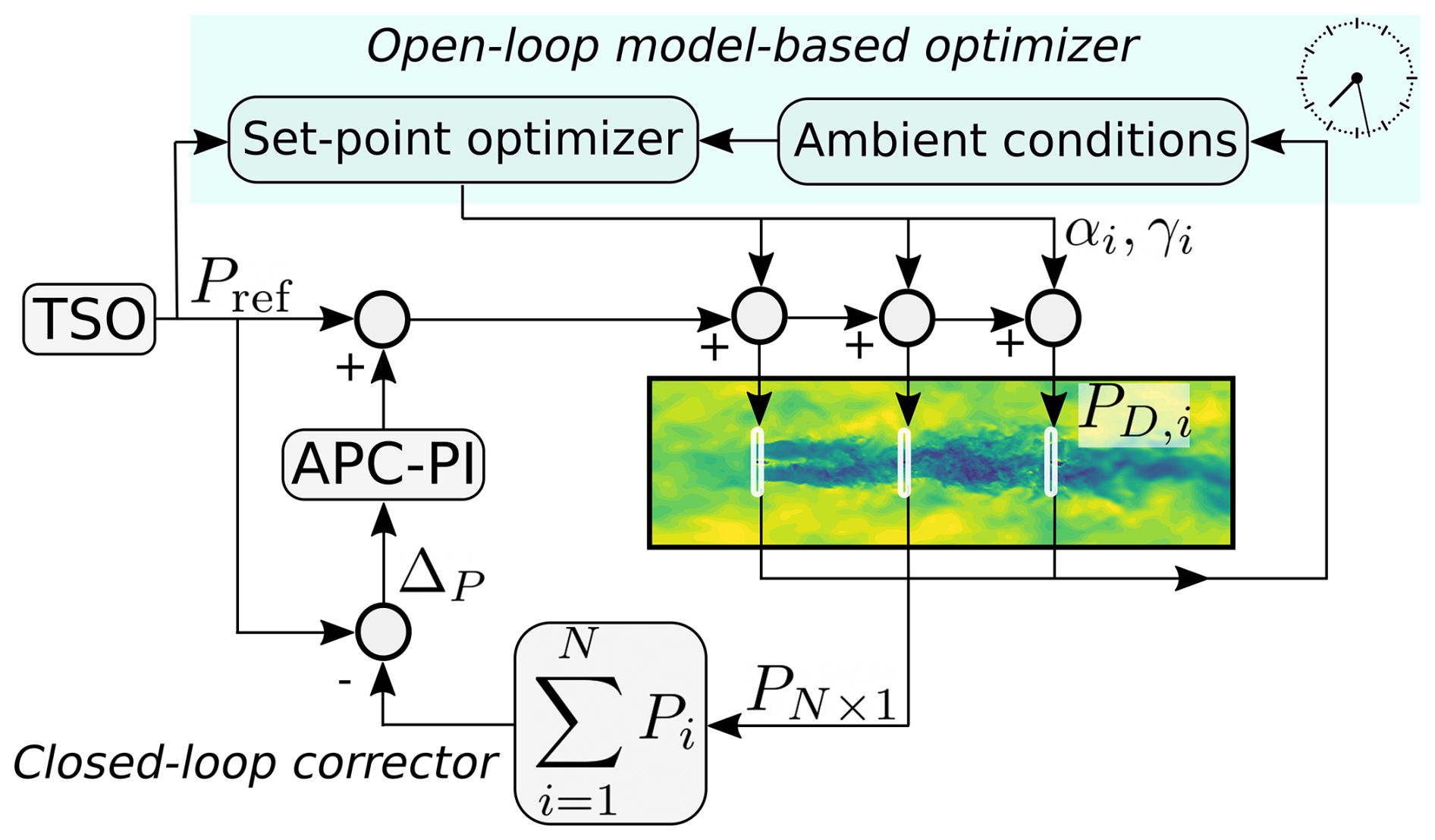
Figure 1 Schematic representation of the APC controller, featuring an open-loop model-based optimizer and a closed-loop corrector.

The closed and open loops operate at different time rates due to the varying timescales of the physical phenomena they control. Specifically, the open loop, which adjusts the yaw setpoints γ_i and power shares α_i, updates at a slow rate because of the time required by wakes to propagate downstream. On the other hand, the closed loop operates at a much faster rate, as it is charged with locally correcting small tracking errors. In this study, the open loop is updated 3 orders of magnitude faster than the closed loop.

2.1.1 Open-loop setpoint optimal scheduler

The open-loop part of the algorithm calculates the optimal setpoints for yaw misalignment and power share. These are determined by solving an optimization problem that maximizes the minimum power reserve across the farm, while meeting a specified overall power demand. All necessary flow-related quantities are computed from a fast engineering model, which in this work is based on the FLORIS v3 implementation (NREL, 2023). The optimization is based on a gradient-based approach (Brayton et al., 1979). In fact, this class of methods typically outperforms derivative-free approaches (Thomas et al., 2023) in the presence of active constraints at convergence (the power demand, in this case) and when the solution space is smooth (Nocedal and Wright, 2006).

The power of the ith turbine is noted as $P_i=P_i({\mathbf{A}}_i,{\mathit{u}}_i)$, where ${\mathbf{A}}_i=(U,\mathit{\psi },k,I)$ indicates the local ambient conditions, here assumed to include the rotor-equivalent wind speed U, wind direction ψ, vertical shear k, and turbulence intensity (TI) I. The symbol ${\mathit{u}}_i=({\mathit{\gamma }}_i,{\mathit{\alpha }}_i)$ indicates the control inputs, which are represented by the yaw misalignment γ_i and power share ${\mathit{\alpha }}_i=P_{\mathrm{D},i}/{\sum }_{i=\mathrm{1}}^N{P}_{\mathrm{D},i}$, where P_D,i is the power demand. Power is computed using the wind farm flow model described in Sect. 2.5. The power of misaligned and curtailed wind turbines is computed based on Tamaro et al. (2024a).

The maximum power that turbine i can capture by modifying its control setpoints u_i (with the setpoints of the other turbines held constant) is calculated as

$$\begin{array}{}\text{(1)}& P_{\mathrm{a},i}=\underset{{\mathit{u}}_i}{max}{P}_i({\mathbf{A}}_i,{\mathit{u}}_i)={\displaystyle \frac{\mathrm{1}}{\mathrm{2}}}\mathit{\rho }\mathit{\pi }{R}^{\mathrm{2}}{U}^{\mathrm{3}}{C}_{\mathrm{P}}(\mathit{\lambda },\mathit{\theta },\mathit{\gamma }),\end{array}$$

where ρ is the air density, R is the rotor radius, $C_{\mathrm{P}}(\mathit{\lambda },\mathit{\theta },\mathit{\gamma })$ is the power coefficient, and $\mathit{\lambda }=\mathrm{\Omega }R/U$ is the tip speed ratio (where Ω is the rotor speed and θ is the blade pitch angle).

Following Tamaro et al. (2024a) (Sect. 3.2), the power coefficient is calculated as

$$\begin{array}{}\text{(2)}& C_{\mathrm{P}}(\mathit{\lambda },\mathit{\theta },\mathit{\gamma })=C_{\mathrm{P}}(\mathit{\lambda },\mathit{\theta },\mathrm{0}){\mathit{\eta }}_{\mathrm{P}}(\mathit{\lambda },\mathit{\theta },\mathit{\gamma }),\end{array}$$

where $C_{\mathrm{P}}(\mathit{\lambda },\mathit{\theta },\mathrm{0})$ is the power coefficient in wind-aligned conditions and η_P indicates the scaling factor that accounts for power losses due to misalignment γ. This model can also take into account the effects resulting from rotor tilt δ (Tamaro et al., 2024a).

As explained in more detail in Tamaro et al. (2024a), the power model accounts for the turbine-level control strategy. In fact, given the desired power setpoint α_i, misalignment angle γ_i and present wind speed U, the tip speed ratio λ and pitch setting θ appearing in the power model Eq. (2) are computed based on the turbine control strategy. The turbine controller used here is described in Sect. 2.5, although the approach is agnostic to these specific details, and other control approaches could be readily used as well.

The algorithm seeks the setpoint combination that minimizes the maximum power ratio $P_i/P_{\mathrm{a},i}$ across all N turbines in the farm, while ensuring the power demand of the TSO, noted as P_ref, is met. This can be expressed as

$$\begin{array}{}\text{(3)}& \underset{\mathit{u}}{min}\underset{i\in [\mathrm{1},N]}{max}{\displaystyle \frac{P_i}{P_{\mathrm{a},i}}}\text{ such that }\sum _{i=\mathrm{1}}^N{P}_i=P_{\mathrm{ref}}.\end{array}$$

In fact, a smaller power ratio $P_i/P_{\mathrm{a},i}$ results in a larger reserve $r_i=\mathrm{1}-P_i/P_{\mathrm{a},i}$, which can be used to mitigate local drops in wind.

Equation (3) represents a constrained optimization problem. However, this optimization does not need to be carried out in real time during operation. Instead, it is performed offline for a range of ambient conditions and wind farm curtailment levels. The results are stored in a lookup table, which is then interpolated at runtime, similarly to the approach used in power-boosting wind farm control (Meyers et al., 2022). Although executing the optimization online may be feasible, performing it offline offers the advantage of validating the resulting setpoints in advance, which is beneficial from an operational safety perspective. When the maximum reserve of the farm is zero, the optimization provides the traditional maximum power solution (Meyers et al., 2022), making power boosting a limiting case of the proposed APC formulation. This feature ensures a seamless and smooth transition between the power boosting and APC modes of operation.

By using a load surrogate model (Guilloré et al., 2024), damage could be readily introduced as a cost term or a constraint in the optimization, although this option was not considered further in this work.

2.1.2 Closed-loop corrector

The closed-loop corrector is directly adopted from the work of van Wingerden et al. (2017). It features a simple PI feedback loop that operates based on the power tracking error, which results from the open-loop part of the control system. The tracking error Δ_P is defined in this work as

$$\begin{array}{}\text{(4)}& {\mathrm{\Delta }}_{\mathrm{P}}=P_{\mathrm{ref}}-\sum _{i=\mathrm{1}}^N{P}_i.\end{array}$$

The PI gains are obtained with a tuning procedure based on a simple Simulink (The MathWorks Inc., 2022) model described in Sect. 2.6; van Wingerden et al. (2017) proposed a gain scheduling based on the number of saturated turbines. This approach is not used here because it was found that – when used with a limited number of wind turbines – it may cause abrupt variations in the gains that can lead to instabilities. Instead, when a turbine saturates, its local power tracking error is redistributed equally among the non-saturated ones, as proposed by Vali et al. (2019). This is explained in more detail in Sect. 2.3.

The controller features an anti-windup term on the integrator when all turbines are saturated, and the integrator is reset when no saturation occurs, as proposed by Silva et al. (2022).

2.2 Reference APC formulations for performance comparison

Three reference wind farm APCs are considered, with the goal of comparing the performance of the proposed power-reserve-boosting method, namely:

• Open loop (OL). This simple approach assigns predetermined setpoints α_i to each turbine as fractions of the power demanded by the TSO, so that ${\sum }_{i=\mathrm{1}}^N{\mathit{\alpha }}_i=\mathrm{1}$. These setpoints are scheduled with the current wind direction to account for different local power availabilities, but they are independent of P_ref.

• Closed loop (CL). This method is the same as OL with the addition of the PI feedback loop described in Sect. 2.1.2.

• Closed loop with load balance (CL+LB). This method consists of CL without the fixed scheduling of the power share setpoints α_i. Instead, an additional PI loop is nested to distribute the α_i's, with the purpose of balancing loads throughout the wind farm (Vali et al., 2019). In this work, the tower-base fore–aft bending moment is chosen as the target load. As proposed by Silva et al. (2022), the mean load is computed considering only non-saturated turbines, and an anti-windup term is added to the integrator of a turbine when it saturates.

All open-loop setpoints are computed based on the engineering model of the plant (NREL, 2023). CL, CL+LB, and CL+MR feature the same PI control block described in Sect. 2.1.2, so the closed-loop part is exactly the same. A visual comparison of all APC strategies considered in this work is presented in Fig. 2.

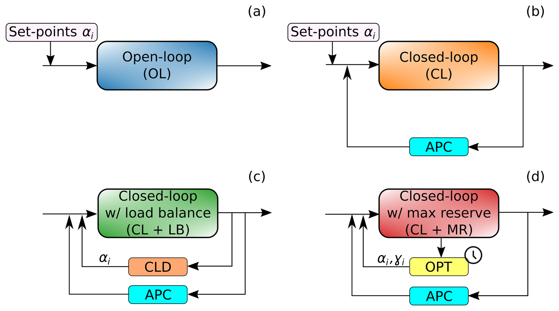
Figure 2 Visual comparison of the three APCs considered in this work: open loop (a), closed loop (b), and closed loop with load-balancing setpoint distributor (c) and closed loop with max-reserve setpoint distributor (d).

2.3 Identification and treatment of saturation conditions

Local turbine saturations are detected when the blade pitch lies at its optimal value and the tracking error exceeds a given threshold, set to 1 % of rated power. Both conditions need to be verified to activate saturation. The threshold for the pitch angle is set to 0.4°. When a wind turbine enters saturation, its power demand is fixed to the last value recorded, while its local tracking error is equally redistributed to non-saturated turbines in the form of an additional power demand to ensure that ${\sum }_{i=\mathrm{1}}^N{\mathit{\alpha }}_i=\mathrm{1}$. This way, locally isolated saturation events – even if persistent – do not introduce significant tracking errors as long as other turbines with enough power reserve can compensate.

On the other hand, conditions in which all wind turbines are close to saturation are particularly harmful to the tracking accuracy, as a cascade effect can be triggered that may lead to all turbines being saturated. In fact, in this case, all wind turbines operate in greedy mode and, if the TSO demand drops, a significant (negative with respect to Eq. 4) tracking error will arise. To avoid this situation, when the wind farm produces more than the instantaneous demand (with a threshold set to 3 % of the rated power), every saturation condition is forcibly reset.

2.4 Wind turbine controller

The wind turbine controller is characterized by two distinct regimes, namely:

• Below rated. The blades lie at the optimal pitch angle, while the generator torque Q is related to the rotor speed Ω as Q(Ω)=κΩ², where κ is a constant (Bossanyi, 2000).

• Above rated. Each turbine yields its demanded power by collectively pitching the blades based on a standard PI loop. Q and Ω are fixed and equal to the rated values, i.e., Q_R and Ω_R, respectively.

An intermediate regime is also often present in typical controllers for noise or load reduction (e.g., thrust clipping) (Abbas et al., 2022); however, such an intermediate control regime is not considered in this work for simplicity.

The transition between the below- and above-rated regimes occurs when Ω exceeds Ω_R. Turbines can track a given power demand P_D=α_iP_ref by adjusting Ω_R as

$$\begin{array}{}\text{(5)}& {\mathrm{\Omega }}_{\mathrm{R}}=\sqrt[\mathrm{3}]{{\displaystyle \frac{P_{\mathrm{D}}}{\mathit{\kappa }}}}\end{array}$$

and by setting $Q_{\mathrm{R}}=P_{\mathrm{D}}/{\mathrm{\Omega }}_{\mathrm{R}}$. In case a gearbox is present, the rotor angular velocity should be corrected by the gearbox ratio to yield the high-speed shaft velocity.

With this control approach, the blade pitch angle θ can be used to measure the margin of a curtailed wind turbine (Tamaro and Bottasso, 2023). Generally, high values of θ indicate a high margin since the turbine operates at a suboptimal C_P. The lowest limit for θ is the optimal pitch angle θ_opt, which yields the maximum C_P.

This type of controller was chosen because it explicitly receives a power demand as an input, which is accurately tracked using the blade pitch angle. Other control methods could also be used, possibly significantly affecting the APC performance.

2.5 Steady-state model for control synthesis

The engineering farm flow model FLORIS v3 (NREL, 2023) is used both to synthesize the open-loop part of the controller and to perform steady-state analyses. The results reported here are based on the Gauss–curl hybrid wake model with default wake parameters, due to its fast computation time and accurate modeling of lateral wake deflection (King et al., 2021). To model off-rated operation, the lookup tables of power coefficient C_P and thrust coefficient C_T are modified to consider curtailed conditions. The sum of squares freestream superposition model by Katic et al. (1987) and Annoni et al. (2018) is used to model the interaction of the wakes.

Since off-rated operation spans a wide range of C_T – and misaligned operation is strongly dependent on C_T (Cossu, 2021; Heck et al., 2023) – the standard FLORIS model is coupled with an analytical model to predict rotor performance (Tamaro et al., 2024a), rather than relying on the ${\cos }^{p_p}$ method (Liew et al., 2020). In fact, the latter may yield inaccurate power estimates in the scenarios considered here, as it neglects to consider how the rotor is controlled as it is yawed out of the wind. Conversely, the misalignment model by Tamaro et al. (2024a) determines how much power is lost for a given misalignment angle γ based on the tip speed ratio λ and pitch setting θ used by the turbine. Since λ and θ are the results of the control strategy, which is itself reacting to γ, the problem is implicit. Hence, to compute $C_{\mathrm{P}}=C_{\mathrm{P}}(\mathit{\lambda },\mathit{\theta },\mathit{\gamma })$ and $C_{\mathrm{T}}=C_{\mathrm{T}}(\mathit{\lambda },\mathit{\theta },\mathit{\gamma })$, the balance equation between aerodynamic power P and demanded power P_D is solved iteratively. Following Tamaro et al. (2024a), the equation

$$\begin{array}{}\text{(6)}& P={\displaystyle \frac{\mathrm{1}}{\mathrm{2}}}\mathit{\rho }\mathit{\pi }{R}^{\mathrm{2}}{U}^{\mathrm{3}}{C}_{\mathrm{P}}(\mathit{\lambda },\mathit{\theta },\mathit{\gamma })=Q(P_{\mathrm{D}},\mathrm{\Omega })\mathrm{\Omega }=P_{\mathrm{D}}\end{array}$$

is solved for λ with θ=θ_opt. If the resultant Ω is smaller than the rated value Ω_R – which is computed from P_D via Eq. (5) – the turbine operates in below-rated conditions, whereas if Ω≥Ω_R it is in rated conditions. In this case, Eq. (6) is instead solved for θ, with $\mathit{\lambda }={\mathrm{\Omega }}_{\mathrm{R}}R/U$.

In the optimization phase, we normalize P_D using the rated power P_R, defining a curtailment parameter $\mathit{ϵ}=P_{\mathrm{D}}/P_{\mathrm{R}}$. Figure 3 presents the setpoints of λ and θ for a range of ϵ values for U=8 m s⁻¹, plotted as functions of the misalignment γ.

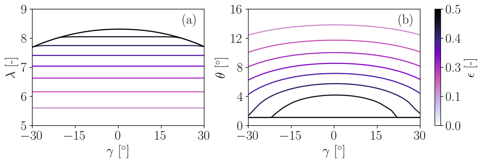
Figure 3 Control setpoints λ (a) and θ (b) plotted as functions of the misalignment angle γ for U=8 m s⁻¹ and for different values of the normalized power demand ϵ, as indicated by the different colors of the lines.

Figure 3a shows that when ϵ is decreased, λ is reduced due to the smaller Ω_R (see Eq. 5). Accordingly, the blade pitch angle in Fig. 3b increases to reduce the power output.

The quantities ϵ and γ are used as optimization variables. The curtailment ϵ is limited to $\mathrm{0}\le {\mathit{ϵ}}_i\le P_{\mathrm{a},i}/P_{\mathrm{R}}$ to ensure that the optimizer never asks for a power demand that exceeds the locally available one, while the yaw angle is bounded to ${\mathit{\gamma }}_{\min }\le \mathit{\gamma }\le {\mathit{\gamma }}_{\max }$; these turbine-dependent limits are typically imposed by ultimate and/or fatigue loads.

A different optimization is solved for each ambient condition (wind speed, wind direction, optionally turbulence intensity) to generate the associated setpoints. When the optimization converges, the resulting power share setpoints are computed as ${\mathit{\alpha }}_i=P_i/{\sum }_{i=\mathrm{1}}^N{P}_i$, and they are stored together with the yaw setpoints in a lookup table. The optimization problem is solved with the gradient-based sequential quadratic programming (SQP) method (Brayton et al., 1979). A total of 102 optimizations are performed, i.e., 51 per wind direction, each corresponding to a wind farm power request from 50 % to 100 % of the greedy one. During operation, α_i and γ_i are linearly interpolated from the lookup tables based on the average power demand computed over the last 30 seconds. Clipping to the last available value of the lookup table is applied to avoid extrapolation.

Figure 4 reports the yaw setpoints and power share percentages that maximize the minimum local available power for the aligned turbines of Sect. 3.1.

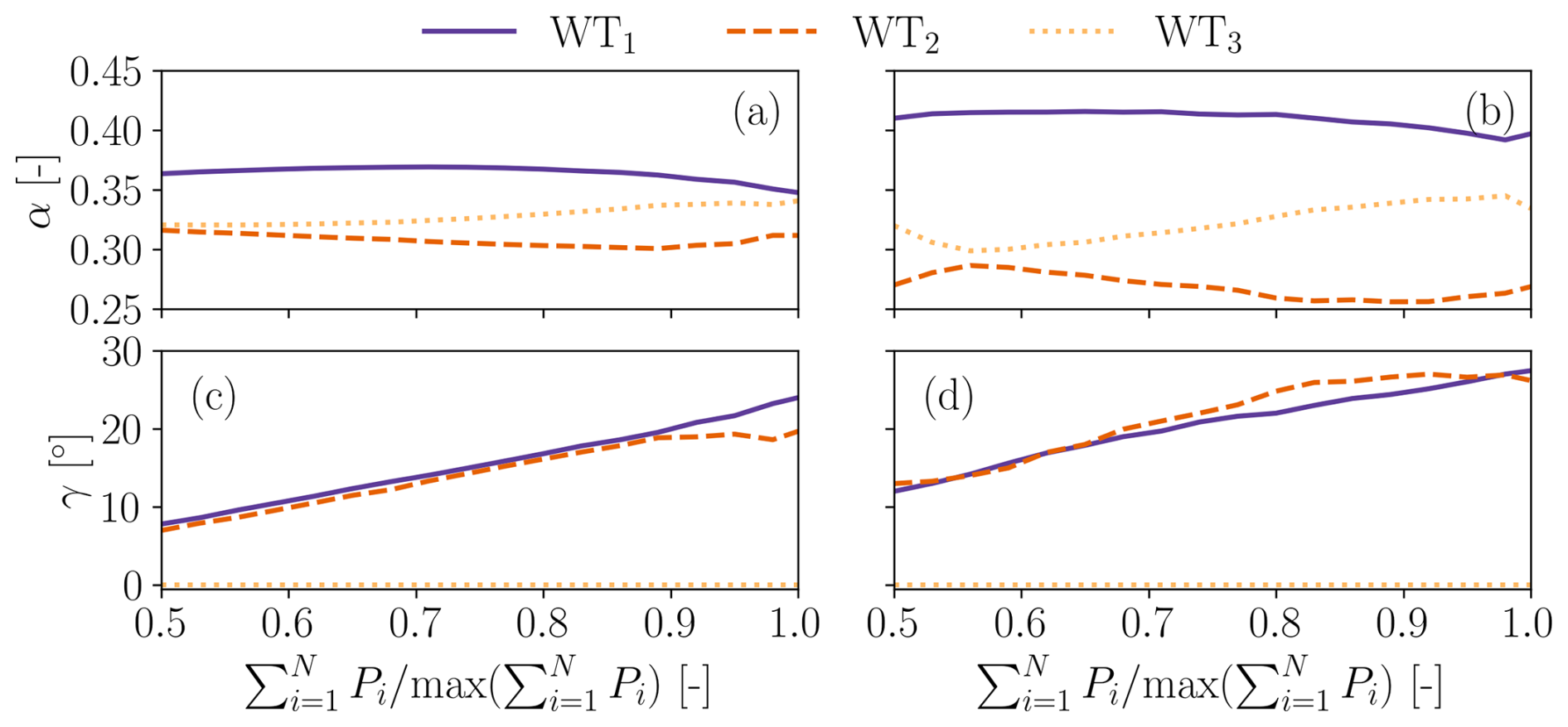
Figure 4 Optimal setpoints that maximize the minimum power reserve for the three aligned turbines of Sect. 3.1. Power setpoints (a, b), yaw setpoints (c, d). Wind direction ψ=7.1° (50 % wake overlap) (a, c), wind direction ψ=3.6° (75 % wake overlap) (b, d). The power setpoints are plotted as fractions of the available wind farm power.

The figure shows that the most upstream turbines are misaligned with respect to the wind, with the goal of increasing the power reserves of the downstream ones. The wind turbines are misaligned more when the rotor overlap is larger. The power shares result from different local inflow conditions, yaw misalignment, and wake effects.

2.6 Digital twin for gain tuning

The gains of the APC controllers are synthesized with a reduced wind turbine model coupled with a simple dynamic wake model. The Simulink (The MathWorks Inc., 2022) implementation features three wind turbines with their own controllers. The Jensen wake model (Jensen, 1983) is combined with the instantaneous thrust coefficient C_T to estimate the wake deficit for downstream wind turbines. Wake effects are delayed based on the local wind speed and wind turbine separation distance to simulate the time needed for wake effects to propagate downstream. Figure 5 presents a sketch of the digital twin. This rather crude wake model is adopted here purely because, although very simple, it still provides for a realistic estimation of wake deficit in this aligned setup, although probably not necessary for the goal of gain tuning; it is, however, clear that other more sophisticated models could be used.

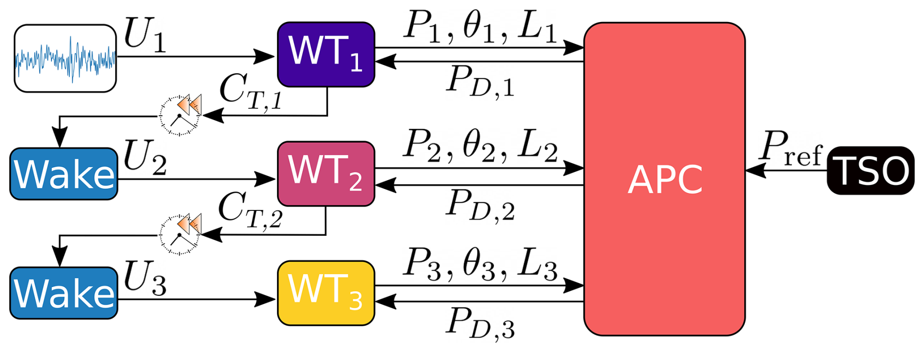
Figure 5 Block diagram of the structure of the Simulink model used for optimizing the APC gains.

The wind turbines are assumed to be fully aligned, and the inflow is taken from wind tunnel measurements in a turbulent boundary layer. The CL and CL+LB APC super-controllers are implemented in the digital twin. Their gains are optimized with the interior-point gradient-based algorithm, where the cost function is the root mean square (RMS) of the power tracking error. To improve the robustness of the gains, zero-mean white noise is added to the input measured power.

In the case of CL+LB, the cost function is defined as $J=\mathrm{0.75}{\stackrel{\mathrm{‾}}{\mathrm{\Delta }}}_{\mathrm{P}}+\mathrm{0.25}{\sum }_{i=\mathrm{1}}^N{\stackrel{\mathrm{‾}}{\mathrm{\Delta }}}_{\mathrm{L},i}$, and it represents the weighted sum of the non-dimensional tracking error ${\stackrel{\mathrm{‾}}{\mathrm{\Delta }}}_{\mathrm{P}}$ and non-dimensional overall load-balancing error ${\stackrel{\mathrm{‾}}{\mathrm{\Delta }}}_{\mathrm{L},i}$, defined as ${\stackrel{\mathrm{‾}}{\mathrm{\Delta }}}_{\mathrm{L},i}=L_i-{\sum }_{i=\mathrm{1}}^N{L}_i$. Both quantities are non-dimensionalized to lie in the interval [0,1].

3 Results

3.1 Numerical setup

Tests are performed on an array of three wind turbines located at a streamwise distance of 4 diameters (4D). The use of a small cluster of turbines is motivated by the computational cost of the LES-ALM simulations. However, the small distance between the turbines implies a short propagation time that requires a very robust APC. At the same time, this layout – while still capturing the strong aerodynamic couplings caused by single and double wake interactions on downstream rotors – is sufficiently simple to clearly isolate and understand the underlying effects within the wind farm.

Two scenarios are considered, with wind directions ψ equal to 3.6 and 7.1°, corresponding to 75 % and 50 % rotor overlaps, respectively. Rotor overlap is defined as the lateral offset between the centers of two wind turbine rotors, expressed as a percentage of the rotor diameter. An overlap of 100 % means that the rotors are perfectly aligned (center to center), while 50 % overlap means that the downstream rotor is laterally displaced by half a rotor diameter. These scenarios were chosen because they involve partial wake impingement, which is particularly relevant for fatigue considerations (Guilloré et al., 2024). The most upstream turbine is labeled WT₁, the most downstream one WT₃, and the one in the center is referred to as WT₂. Simulations are conducted using the IEA 3.4 MW reference wind turbine, a typical onshore machine with a contemporary design (Bortolotti et al., 2019). Here, we only note that the turbine has a rotor diameter D of 130 m and a 5° uptilt angle (i.e., $\mathit{\delta }=-\mathrm{5}\mathit{°}$) (Tamaro et al., 2024a). The optimal pitch is θ_opt=1.09°, and the constant κ for the generator torque in the below-rated regime is κ=1804 kN m s² rad⁻². The maximum yaw rate is equal to 0.8 ° s⁻¹. The PI gains for the CL+MR controller are $K_{\mathrm{APC}}^{\mathrm{P}}=\mathrm{1.3127}$ [–] and $K_{\mathrm{APC}}^{\mathrm{I}}=\mathrm{0.2063}$ s⁻¹, while the ones for the coordinated load distribution (CLD) of CL+LB are $K_{\mathrm{CLD}}^{\mathrm{P}}=\mathrm{0.03427}$ Nm⁻¹ and $K_{\mathrm{CLD}}^{\mathrm{I}}=\mathrm{0.07959}$ Nm⁻¹ s⁻¹. The APC open loop is updated every 30 s and the closed loop every 0.01 seconds. The closed-loop frequency of 100 Hz is faster than the 1–10 Hz reported by other studies (Liu et al., 2019; Vali et al., 2019), and it is due to the small time step used by the LES-ALM solver. In CL+LB, loads are filtered by applying exponential smoothing with a time constant of 0.1 s.

LES-ALM simulations are used for testing the performance of the new APC formulation, because they can represent the complex dynamics typical of wind turbine wakes and their interactions (Wang et al., 2019). We use an in-house version of the LES-ALM code SOWFA (Troldborg et al., 2007; Wang, 2021), which includes the smearing correction to the blade tip forces proposed by Meyer Forsting et al. (2019). The incompressible solver is based on a finite-volume formulation and uses a standard Smagorinsky model to treat subgrid scales, with a constant of 0.13 (Sagaut, 2006).

The LES Cartesian mesh comprises approximately 14.3×10⁶ cells and includes six refinement levels. The smallest cells measure 1 m and are located in correspondence with the three rotors. Two tilted hexahedral regions are used to refine the wind farm array. The computational domain, grids, and turbine layout are shown in Fig. 6.

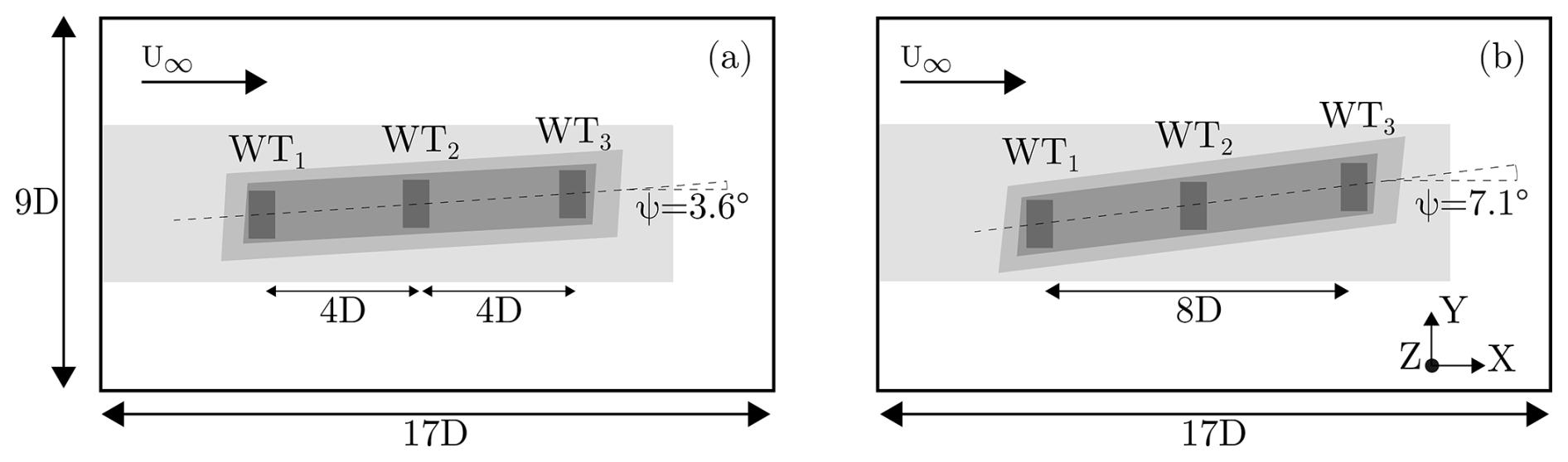
Figure 6 Wind farm layout and simulation scenarios for 75 % (a) and 50 % (b) rotor overlap. The shaded areas indicate the mesh refinement levels.

Unsteady tests are run with a turbulent wind obtained from a precursor generated in stable atmospheric conditions with periodic inlet–outlet boundary conditions. The inflow is characterized by a turbulence intensity TI =5.7 %, a hub height wind speed U_∞=9.54 m s⁻¹, a power-law shear coefficient k=0.21, and an integral length scale of turbulence at hub height equal to 0.79D. The normalized mean streamwise velocity and turbulence intensity fields at the inlet – 4D upstream of WT₁ – are shown in Fig. 7.

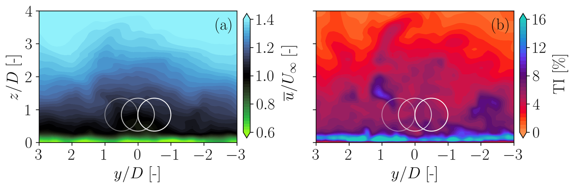
Figure 7 Slices of inflow fields. Time-averaged wind speed normalized by the freestream wind speed (a) and turbulence intensity field (b). The locations of the three wind turbines for ψ=7.1° (50 % wake overlap) are marked with a line transparency that increases along with the distance from the inflow slice.

Each LES-ALM simulation is run for 1200 s. The first 200 s are considered as the initial transient, and hence they are discarded. The total time of 1000 s is approximately equivalent to 1.6 standard 10 min seeds, which is less than the minimum recommended value (Liew and Larsen, 2022) but in line with the numerical study of van Wingerden et al. (2017). The figure shows that the three rotors are immersed in the boundary layer and that the flow is not perfectly uniform, which is expected, given the integral length scale of 0.79D and the averaging time of only 1000 s. Given the short duration, results are likely dependent on the specific inflow realization, especially at high power demands due to the multiple simultaneous saturations. To mitigate this effect, LES-ALM simulations are also performed with all turbines operating in greedy mode. The results of the different APC formulations are then compared to the corresponding greedy results.

3.2 Reference power demand signal

A dynamic reference power signal typical of automatic generation control (AGC) is used as a reference power signal. AGC is the secondary response regime of grid frequency control, and it consists of the modification of the power output of a plant depending on dynamically changing requests by the TSO (Aho et al., 2012). A similar signal has also been considered by other authors (Fleming et al., 2016; van Wingerden et al., 2017; Shapiro et al., 2017; Boersma et al., 2018; Vali et al., 2019). The signal is defined as

$$\begin{array}{}\text{(7)}& P_{\mathrm{ref}}\left(t\right)=P_{\text{greedy}}\left(\mathit{\psi }\right)(b+c{n}_k^{\mathrm{AGC}}(t\left)\right),\end{array}$$

where $n_k^{\mathrm{AGC}}\left(t\right)$ is a normalized perturbation from a standard test signal, P_greedy is the time-averaged available power of the wind farm in greedy conditions, and b and c are parameters that shift and change the amplitude of $n_k^{\mathrm{AGC}}$, respectively. A “ground truth” greedy power output P_greedy is computed from a LES-ALM simulation in which the turbines are aligned with the inflow and operate in greedy power mode (i.e., P_D=P_R, see Sect. 2.4). Figure 8 shows the time history of the normalized perturbation $n_k^{\mathrm{AGC}}$.

Figure 8 Time history of the normalized perturbation signal $n_k^{\mathrm{AGC}}$ of Eq. (7).

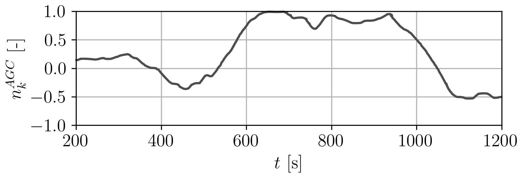
P_greedy is computed on a preliminary LES-ALM simulation under the same ambient conditions of the APC runs, where the turbines operate aligned and in greedy mode. The value c=0.1 is used in all cases, while three different values of b are considered, i.e., $b=[\mathrm{0.7},\mathrm{0.8},\mathrm{0.9}]$. In general, a higher value of b makes the TSO signal harder to track, due to a closer proximity to the greedy power available.

3.3 Steady-state analysis

First, the proposed method CL+MR is compared to OL using the steady-state engineering flow model FLORIS. This analysis is performed on the cluster of three IEA 3.4 MW turbines at a streamwise distance of 4D and three inflow angles $\mathit{\psi }=[\mathrm{0}\mathit{°},\mathrm{3.6}\mathit{°},\mathrm{7.1}\mathit{°}]$, corresponding to rotor overlaps of 100 %, 75 %, and 50 %, respectively.

In addition to this basic comparison to the simplest possible (open-loop) approach, here we also would like to understand the role of wake steering and whether it alone would be sufficient to achieve a satisfactory APC performance. To this end, we consider the situation where the OL power setpoints α_i are superimposed, with the yaw misalignment setpoints that optimize power output, i.e., the classical wake-steering-based power boosting. In principle, this method is attractive due to its simplicity compared to CL+MR, and it similarly incorporates wake steering. This approach is referred to in the following as OL+power boosting.

Results are shown in Fig. 9, where we report the difference between the rotor power and the locally available one, normalized by the rated power. We use this quantity instead of the power reserve r in order to compare the APCs in absolute terms.

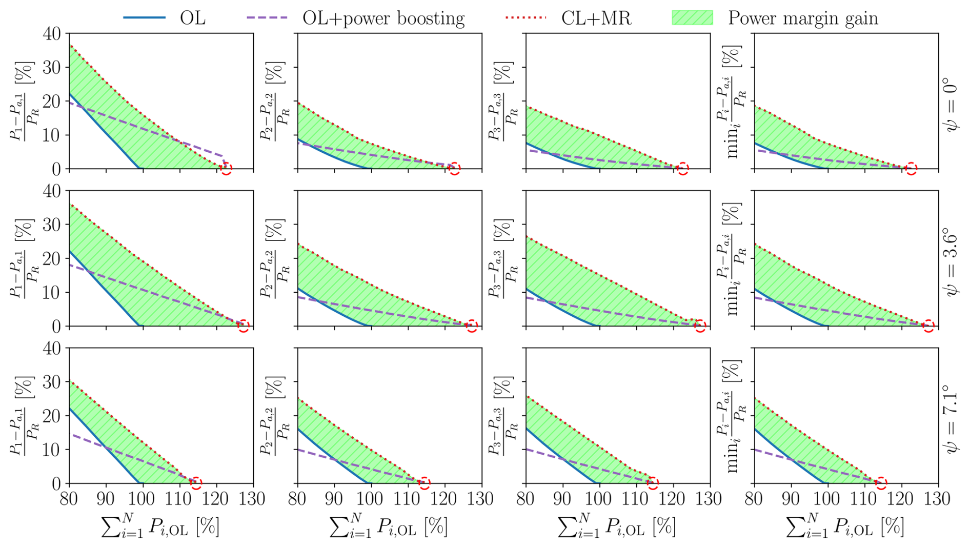
Figure 9 Local power margin in percentage obtained with a purely inductive wind farm control (labeled OL), with an inductive APC that operates with statically misaligned rotors according to the power-boosting solution (labeled OL+power boosting) and with the proposed controller that dispatches power and yaw setpoints to optimize power reserves (labeled CL+MR). The first three columns show the power margin for WT₁, WT₂, and WT₃, respectively, while the fourth column indicates the minimum power margin in the wind farm. The first row is obtained at ψ=0°, i.e., 100 % rotor overlap; the second row at ψ=3.6°, i.e., 75 % rotor overlap; and the third row at ψ=7.1°, i.e., 50 % rotor overlap. On the x axis, wind farm power is normalized by the maximum value for OL. The red circles indicate the classical maximum power solution, and the colored area represents the power reserve improvement of CL+MR with respect to OL.

The figure shows that the margin drops to zero in correspondence with the maximum power of the plant, whereas it increases as the power demand is lowered and the wind turbines are curtailed. Wake steering effectively extends the power available to the wind farm. In agreement with the literature, the effectiveness of wake steering depends on the direction of the wind with respect to the alignment of the turbines, an effect that is here captured by the ψ angle. In all cases, the proposed CL+MR strategy increases the power margin for all wind farm power demands. The highest power margin improvement is observed for ψ=3.6° (75 % wake overlap), and it is in excess of +20 %. As the power demand ${\sum }_{i=\mathrm{1}}^N{P}_{i,\mathrm{OL}}$ is reduced, the added margin of CL+MR diminishes since wake effects get weaker and the effectiveness of wake steering is reduced, in both cases because of the lower C_T. In the figure, the classical maximum power solutions are shown using red circle symbols.

The plots show that OL+power boosting achieves the same power reserve improvement of CL+MR only at the red-circled points, where both the α_i and γ_i setpoints are identical. However, as the wind farm power demand decreases, the power margin of OL+power boosting recovers at a much slower rate than for CL+MR, resulting in a smaller improvement compared to the standard OL approach. At lower power demands – specifically when ${\sum }_{i=\mathrm{1}}^N{P}_{i,\mathrm{OL}}\approx \mathrm{90}\mathit{\%}$ – OL+power boosting actually yields a smaller minimum reserve than OL. This can be attributed to an imbalance in the distribution of power reserves across the wind farm. Specifically, upwind rotors that are yawed for steering their wakes have reduced margins compared to downstream, aligned rotors, which benefit from wake steering. As a result, in CL+MR, the optimizer tends to realign the yawed wake-steering rotors when the power demand drops. Conversely, in OL+power boosting, these rotors remain misaligned: the effectiveness of wake steering diminishes with reducing C_T, which in turn decreases the locally available power. This effect is more pronounced at ψ=7.1° (50 % wake overlap), where wake steering is inherently less effective.

Overall, WT₁ presents the largest power margin for both OL and CL+MR, since it is driven by a clean inflow, while for downstream rotors the margin recovers at a lower rate, due to the non-linear behavior of wake recovery.

3.4 Unsteady conditions

Next, results from the LES-ALM simulations are presented. Figure 10 reports slices of the time-averaged freestream velocity fields $\stackrel{\mathrm{‾}}{u}(x,y)$ at hub height, normalized by the freestream value U_∞. Figure 11 shows the turbulence intensity (TI). The plots are shown for OL, and the proposed CL+MR for ψ=3.6° (75 % wake overlap) and ψ=7.1° (50 % wake overlap) for a power demand level b=0.8. CL and CL+LB are not shown for the sake of simplicity, since they are qualitatively similar to OL.

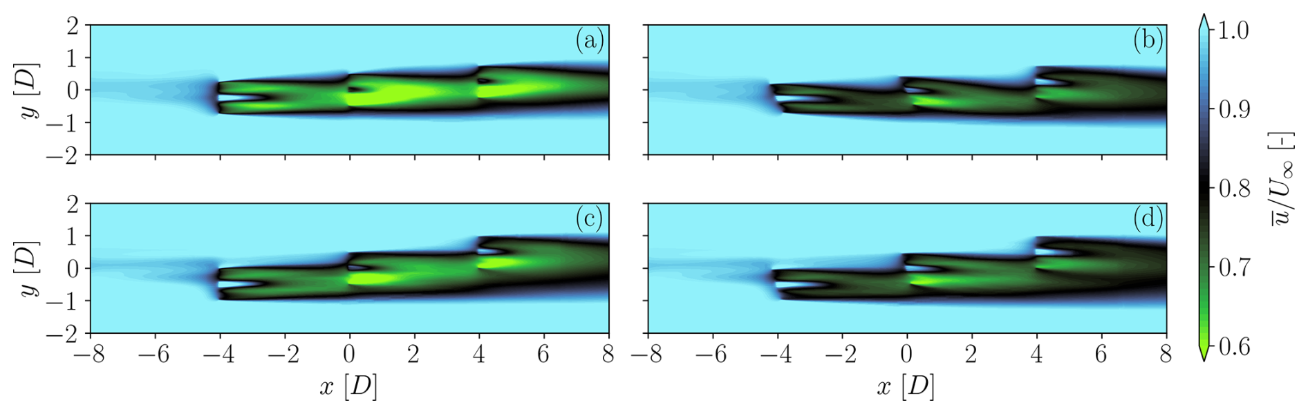
Figure 10 Time-averaged streamwise velocity fields for a TSO power request b=0.8 for two APC control strategies: open loop (OL) (a, c) and closed loop with optimal power reserve (CL+MR) (b, d). ψ=3.6° (75 % wake overlap) (a, b) and ψ=7.1° (50 % wake overlap) (c, d). The slices are extracted at hub height.

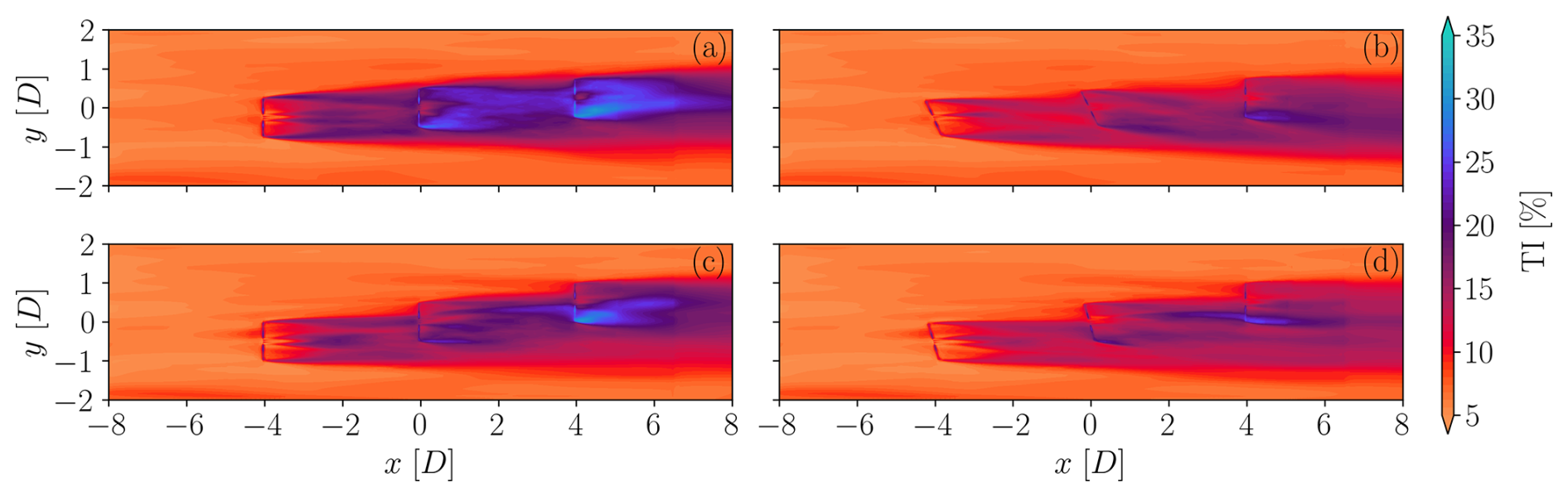
Figure 11 Turbulence intensity fields for a TSO power request b=0.8 for two APC control strategies: open loop (OL) (a, c) and closed loop with optimal power reserve (CL+MR) (b, d). ψ=3.6° (75 % wake overlap) (a, b) and ψ=7.1° (50 % wake overlap) (c, d). The slices are extracted at hub height.

These figures highlight the different extent of wake impingement that occurs on the downstream rotors at ψ=3.6° (75 % wake overlap) and ψ=7.1° (50 % wake overlap). Similarly, Fig. 10b and d allow one to appreciate the effect of yaw misalignment on the wakes, which are significantly deflected to one side compared to fully aligned conditions. The effect is remarkable when considering that the turbines are curtailed, and hence the smaller C_T reduces the deflection compared to a greedy scenario.

The plots of turbulence intensity in Fig. 11 highlight the fact that waked rotors operate in regions of significant turbulence, as expected. The turbulence levels reach rather large values in correspondence with the wake of WT₃, especially in OL with 75 % rotor overlap (see Fig. 11a). Overall, the rather high turbulence intensity levels are likely to be also the result of the unsteady operation of the rotors due to power tracking. For the proposed CL+MR method, the turbulence intensity levels are generally significantly lower than OL for two reasons. First, wake steering reduces wake overlaps, and, second, the rotors operate generally at lower C_T values, which in turn lead to reduced amplitudes of wake meandering (Foti et al., 2018) and to smaller speed gradients over the rotor.

Next, the time series of produced and demanded power are shown in Figs. 12 and 13 for ψ=3.6° (75 % wake overlap) and ψ=7.1° (50 % wake overlap), respectively. The gray background shows the “ground truth” wind farm power from a preliminary LES-ALM simulation where the turbines operate aligned in greedy mode. This greedy power can differ and even be lower than the one produced in the APC cases because of the slightly different wake effects due to curtailment. Nevertheless, it is reported here to provide a proxy for the instantaneous power available in the wind farm.

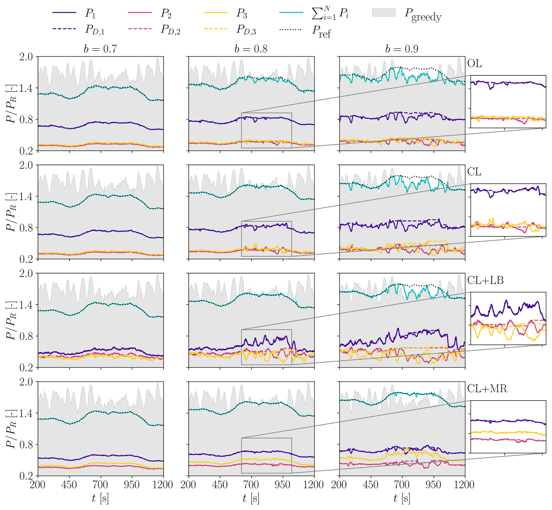
Figure 12 Time series of power demand P_D,i and power-generated P_i for ψ=3.6° (75 % wake overlap). The y axes are non-dimensionalized by the rated power P_R of the IEA 3.4 MW reference wind turbine. The wind farm power obtained in greedy operation (without wake steering) is displayed in the background in gray.

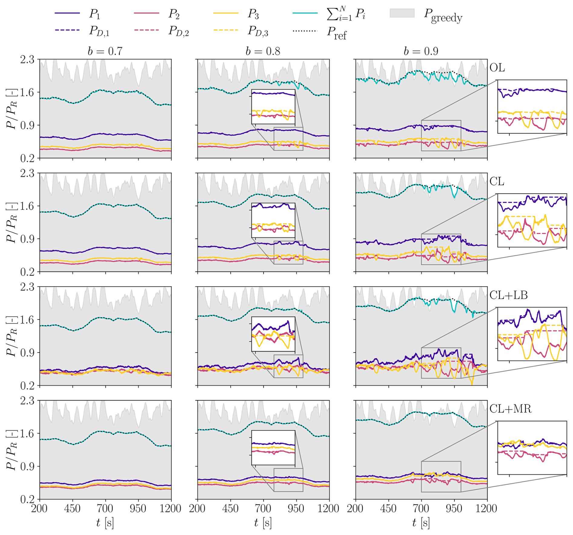
Figure 13 Time series of power demand P_D,i and power-generated P_i for ψ=7.1° (50 % wake overlap). The y axes are non-dimensionalized by the rated power P_R of the IEA 3.4 MW reference wind turbine. The wind farm power obtained in greedy operation (without wake steering) is displayed in the background in gray.

Both figures show that at the low-demand value b=0.7, all methods track power somewhat accurately. In fact, in this case, the power demanded by the TSO is always smaller than the greedy power, and in general, all turbines have enough power reserve to avoid saturations. As the power demand increases, it gets closer to the available one, leading to tracking inaccuracies driven by local saturation events. Still, for b=0.8, the effectiveness of the closed-loop methods is evident. This is mostly due to the setpoint redistribution logic that makes unsaturated turbines compensate for the tracking error of the saturated ones. However, when b>0.8, the power available to the wind farm is often not enough to track the reference signal, and this is especially clear in the time interval 650 s $<t<\mathrm{1000}$ s. In such cases, the higher power availability made possible by wake steering allows only CL+MR to track the signal, while other methods clearly lack the power reserve to do so.

In the zoomed regions of the plots, the saturation events can be clearly observed. In the open-loop case, the power demand remains unaffected since no countermeasure is implemented. Conversely, in the closed-loop cases, the power demand remains constant for saturated rotors since the other ones are called to compensate.

3.4.1 Saturation events

Figures 14 and 15 provide a visual representation of the occurrences of local saturation conditions for each APC strategy and different TSO request scenarios for ψ=3.6° (75 % wake overlap) and ψ=7.1° (50 % wake overlap).

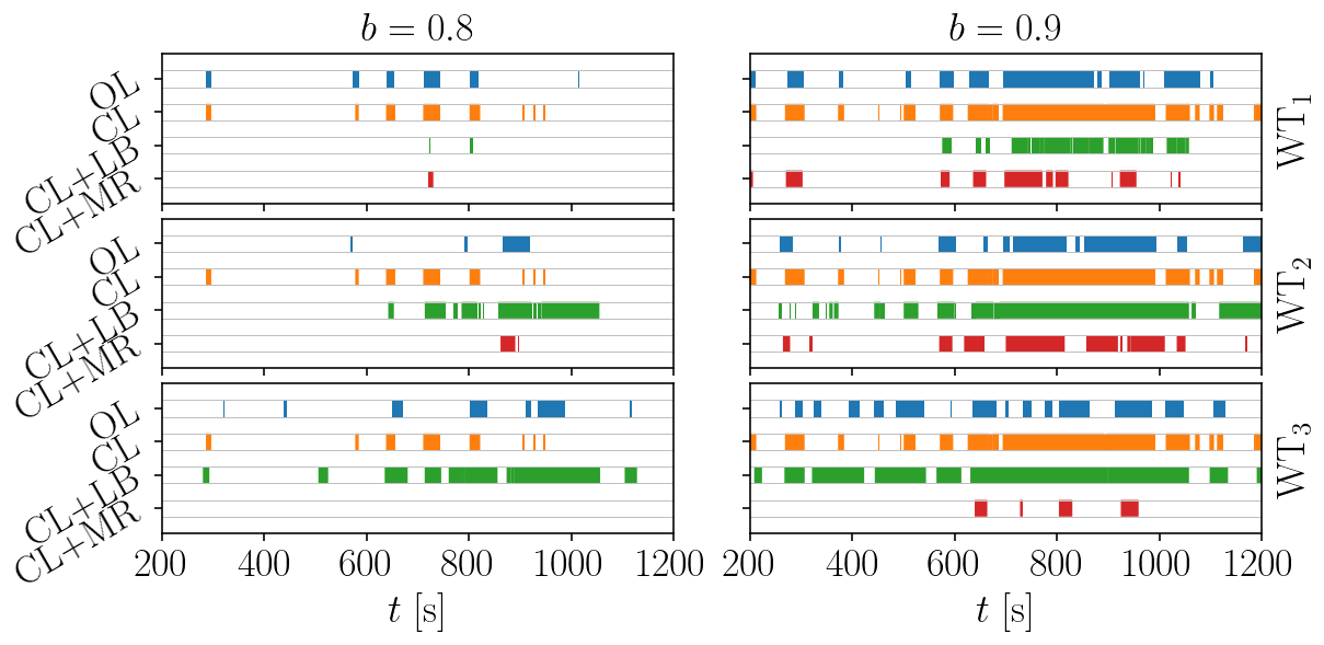
Figure 14 Occurrence of local saturation events for the three turbines in the array and the different control strategies for ψ=3.6° (75 % wake overlap). Only TSO requests with higher demand (b≥0.8) are considered, as few saturations were observed for low-demand values (b=0.7).

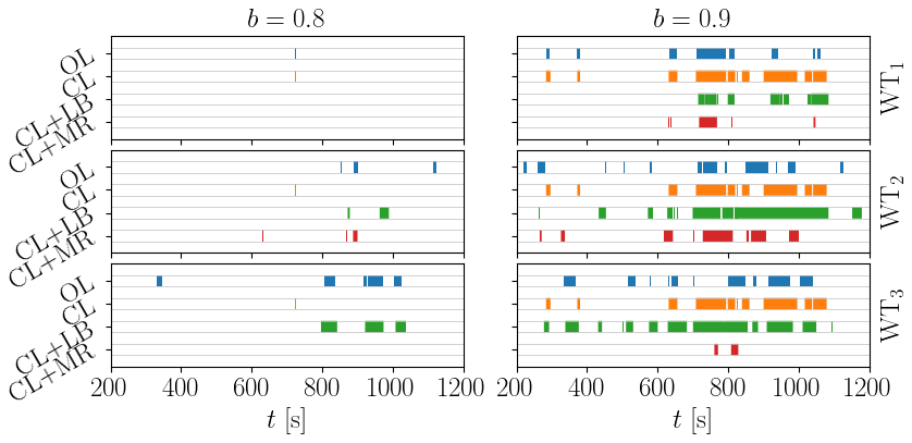
Figure 15 Occurrence of local saturation events for the three turbines in the array and the different control strategies for ψ=7.1° (50 % wake overlap). Only TSO requests with higher demand (b≥0.8) are considered, as few saturations were observed for low-demand values (b=0.7).

These plots indicate that waked wind turbines – i.e., WT₂ and WT₃ – are often saturated because of their generally small power reserve. This effect is exacerbated in the scenario with stronger wake impingement when ψ=3.6° (75 % wake overlap). CL does not reduce the extent of saturation events compared to OL but it rather increases them since other turbines are requested to compensate.

The strategy CL+LB presents the highest number of saturation events of waked turbines. This is because, in order to balance the tower-base fore–aft bending moment, waked turbines are requested to yield a power that is not actually available. At high power demands (i.e., b>0.8), waked wind turbines operate in greedy mode, while WT₁ is responsible for following the TSO signal. In this case, the difference between 50 % and 75 % rotor overlap is remarkable, since in the latter case WT₁ is often saturated, while in the former it is not. This is due to the different wake impingement that modifies the load distribution.

To further understand the reasons for the observed saturation events, the collective blade pitch angle θ is considered. In fact, this parameter can be seen as a proxy of the local power reserve, as discussed in Sect. 2.4. Figures 16 and 17 show the mean collective blade pitch angle $\stackrel{\mathrm{‾}}{\mathit{\theta }}$, binned according to the instantaneous required power and normalized by the available power of the wind farm, as determined from a greedy LES-ALM simulation in the same conditions. This type of binning is chosen to decouple the aerodynamic effects of the APC strategy from sporadic events introduced by the characteristics of the inflow seed. All simulations with different power demand (b) levels are included in the average for a given ψ, and only bins with a minimum total length of 30 s are included. Figure 16 refers to the scenario ψ=3.6° (75 % wake overlap), while Fig. 17 reports the case for ψ=7.1° (50 % wake overlap).

Figure 16 Mean collective blade pitch angle binned by the instantaneous available power, computed from the time series of greedy power and TSO power request for ψ=3.6° (75 % wake overlap). The values represent the means over all tested demands (b values). Only bins with a minimum total length equivalent to 30 s are considered. The optimal blade pitch angle value is indicated by a horizontal black line.

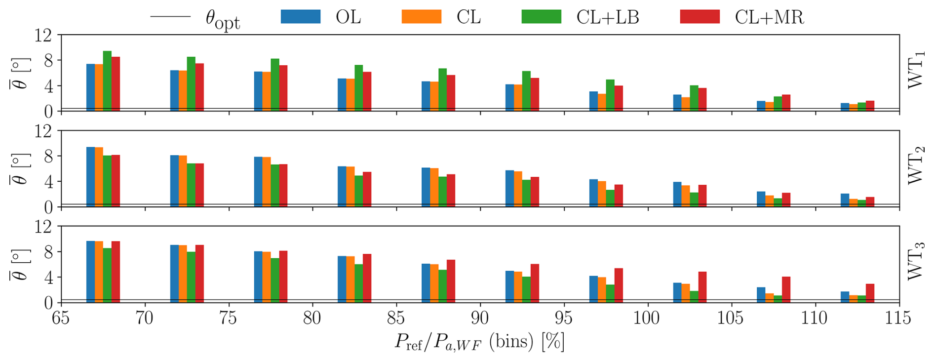
Figure 17 Mean collective blade pitch angle binned by the instantaneous available power, computed from the time series of greedy power and TSO power request for ψ=7.1° (50 % wake overlap). The values represent the means over all tested demands (b values). Only bins with a minimum total length equivalent to 30 s are considered. The optimal blade pitch angle value is indicated by a horizontal black line.

These results show that OL and CL share the same power reserve distribution since, in both cases, the same power setpoints α_i are used. As expected, when the power demand increases, all CL-based methods present a lower $\stackrel{\mathrm{‾}}{\mathit{\theta }}$ than in the OL case; this is due to the closed-loop correction and to the setpoint redistribution that occurs with saturations.

In line with the results shown previously, CL+LB presents a distribution of power reserves that is strongly unbalanced towards the upstream turbine. In fact, the goal of balancing loads implies that waked turbines receive relatively high power demand setpoints, which push them closer to saturation as the power demand increases. This is an important undesired and yet unreported side effect of the load-balancing strategy; as shown later on, in turn, this effect undermines the very ability of the strategy to balance loads in certain situations. The proximity to saturation is visible in Figs. 16 and 17, as the mean blade pitch angles approach the optimum value θ_opt. Conversely, the proposed CL+MR approach presents a distribution of reserves that is balanced throughout the wind farm, resulting in a generally higher power reserve for waked turbines and a lower one for the upstream turbine.

Additionally, CL+LB appears to be sensitive to the wind direction ψ, as a strong wake impingement at ψ=3.6° (75 % wake overlap) yields a more unbalanced power reserve distribution than for ψ=7.1° (50 % wake overlap). Conversely, the effect of the amount of wake overlap is less evident for the proposed CL+MR. This is expected since, in this case, the setpoints specifically depend on the wind direction.

3.4.2 Power tracking accuracy

Figure 18 presents the RMS of the power tracking error Δ_P for both wind direction (i.e., wake overlap) scenarios. Results indicate that closed-loop methods can significantly reduce the tracking error compared to the open-loop approach. The effectiveness is higher for low-demand values b≤0.8 and gradually reduces as the power demand is increased, as it appears already in the time series reported in Figs. 12 and 13. In all cases, the proposed maximum reserve method CL+MR presents the lowest power tracking error. This is to be expected since, for b>0.7, there are short events where the power demand exceeds the available greedy power. Such events degrade the tracking accuracy for methods that do not include wake steering. This highlights the importance of including wake steering in APC, as an effective tool for increasing power reserves.

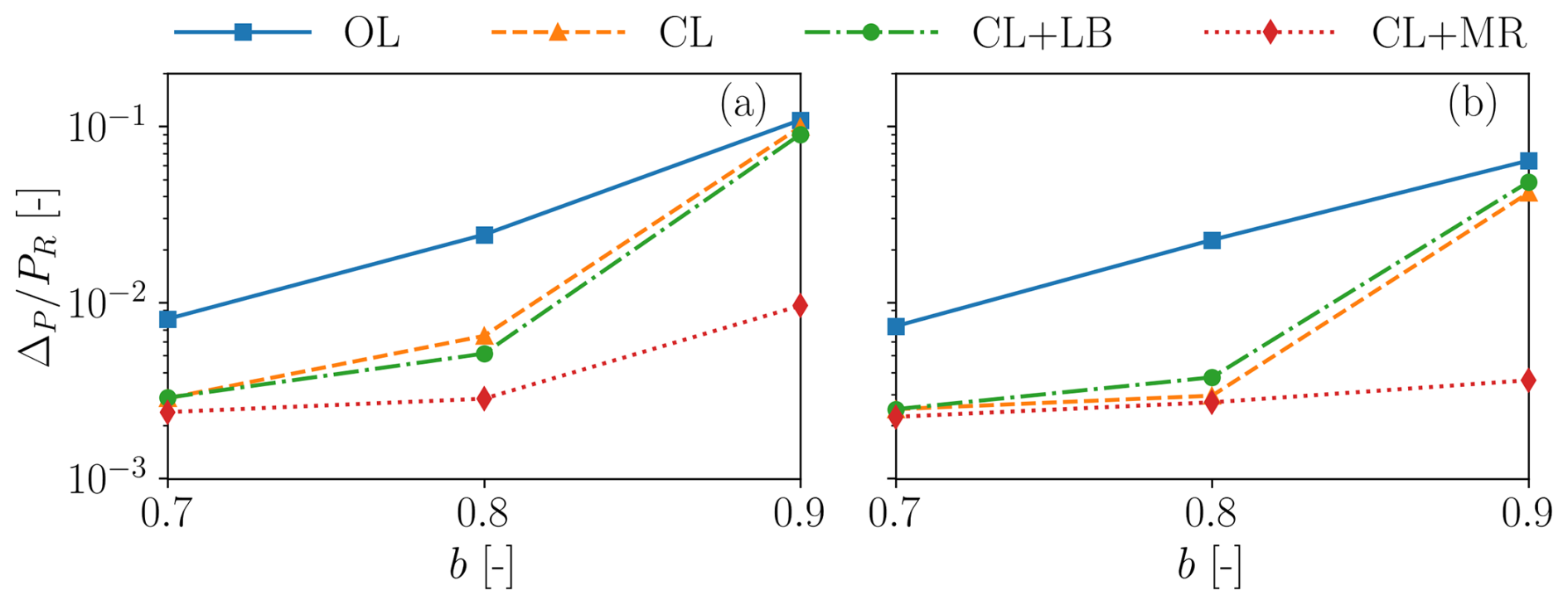
Figure 18 RMS of tracking error normalized by the turbine-rated power, as functions of the TSO demand level (b values). ψ=3.6° (75 % wake overlap) (a); ψ=7.1° (50 % wake overlap) (b).

To perform a more comprehensive comparison, the same analysis is repeated. This time, however, the tracking error time series are binned according to the instantaneous required power normalized by the available power of the wind farm, as done earlier for $\stackrel{\mathrm{‾}}{\mathit{\theta }}$. Only bins with a minimum length of 30 s are considered, and the values of Δ_P in each bin from each power demand scenario (b request) are averaged. Only the positive values of Δ_P are considered here, since they represent a lack of power, i.e., the inability of the plant to deliver what was requested. Results are shown in Figs. 19 and 20 for ψ=3.6° (75 % wake overlap) and ψ=7.1° (50 % wake overlap), respectively.

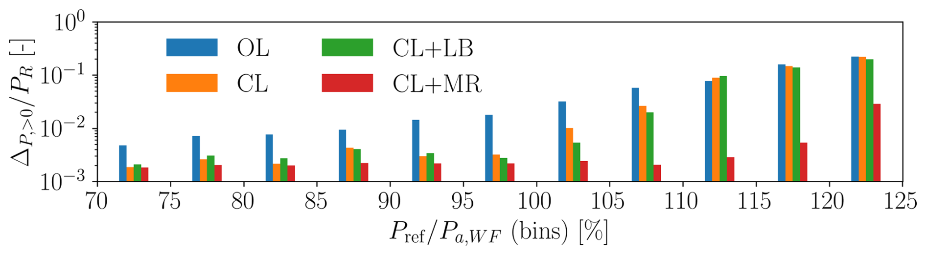
Figure 19 Positive tracking error binned by the instantaneous available power, computed from the time series of greedy power and TSO power request for ψ=3.6° (75 % wake overlap). The values on the y axis are normalized by the rated power of one wind turbine. The values represent the means over all tested demands (b values). Only bins with a minimum total length equivalent to 30 s are considered.

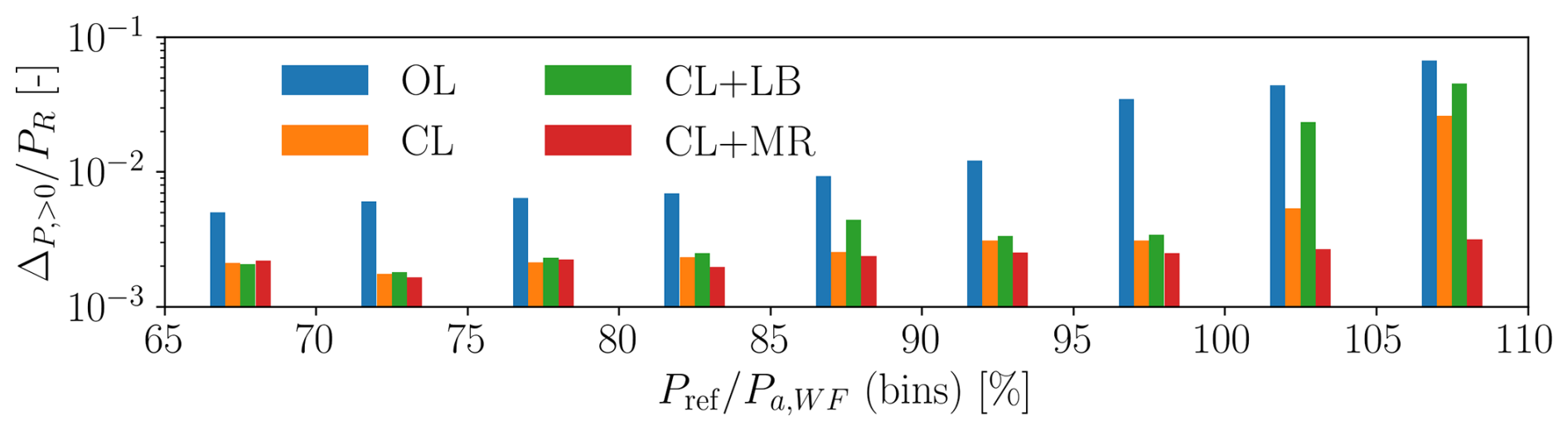
Figure 20 Positive tracking error binned by the instantaneous available power, computed from the time series of greedy power and TSO power request for ψ=7.1° (50 % wake overlap). The values on the y axis are normalized by the rated power of one wind turbine. The values represent the means over all tested demands (b values). Only bins with a minimum total length equivalent to 30 s are considered.

This analysis indicates that all closed-loop methods perform similarly at moderate TSO demands, i.e., b<0.8, with a remarkable performance improvement over OL. The improvement of closed-loop methods is due to the faster response of the wind farm and to the treatment of saturation conditions.

However, as the power demand approaches $P_{\mathrm{ref}}/P_{\mathrm{a},\mathrm{WF}}\approx \mathrm{100}\mathit{\%}$, the proposed CL+MR exhibits a much improved tracking accuracy than all other methods. If, on the one hand, this is to be expected when $P_{\mathrm{ref}}/P_{\mathrm{a},\mathrm{WF}}>\mathrm{100}\mathit{\%}$, due to the overall higher wind farm power, the improvements observed for $\mathrm{80}\mathit{\%}<P_{\mathrm{ref}}/P_{\mathrm{a},\mathrm{WF}}<\mathrm{100}\mathit{\%}$ are less obvious. In fact, since CL, CL+LB, and CL+MR share the exact same closed-loop part of the APC controller, the better performance of the new CL+MR is to be attributed to the more balanced power reserve distribution, consistently with the mean blade pitch angles shown in Figs. 16 and 17. This is also in agreement with the results of the steady-state analysis shown in Sect. 3.3.

3.4.3 Load and fatigue analysis

Here we characterize the performance of the proposed CL+MR strategy on the loading of the turbines, and we compare it to the other reference APC methods.

First, the average loading of the turbines is analyzed by considering the mean tower-base fore–aft bending moment L. Since the turbines are yawing out of the wind when performing wake steering, the moment is computed by always considering the component orthogonal to the rotor orientation. Figures 21 and 22 report the results for the three wind turbines in the array, for the cases ψ=3.6° (75 % wake overlap) and ψ=7.1° (50 % wake overlap), respectively.

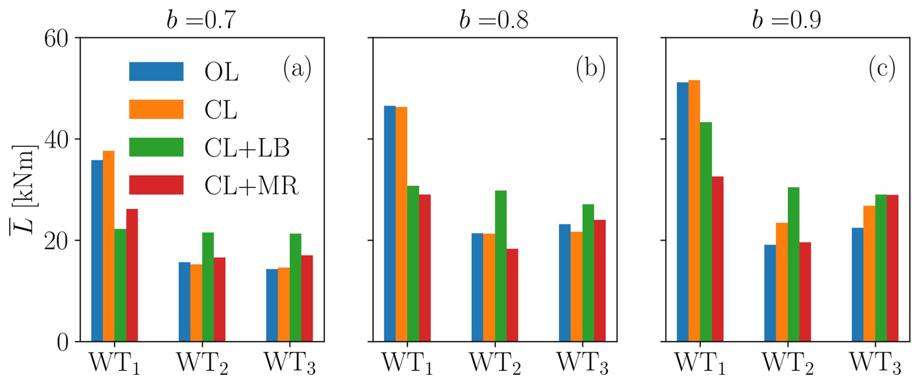
Figure 21 Mean tower-base fore–aft bending moment for the TSO demand levels b=0.7 (a), b=0.8 (b), and b=0.9 (c), for ψ=3.6° (75 % wake overlap).

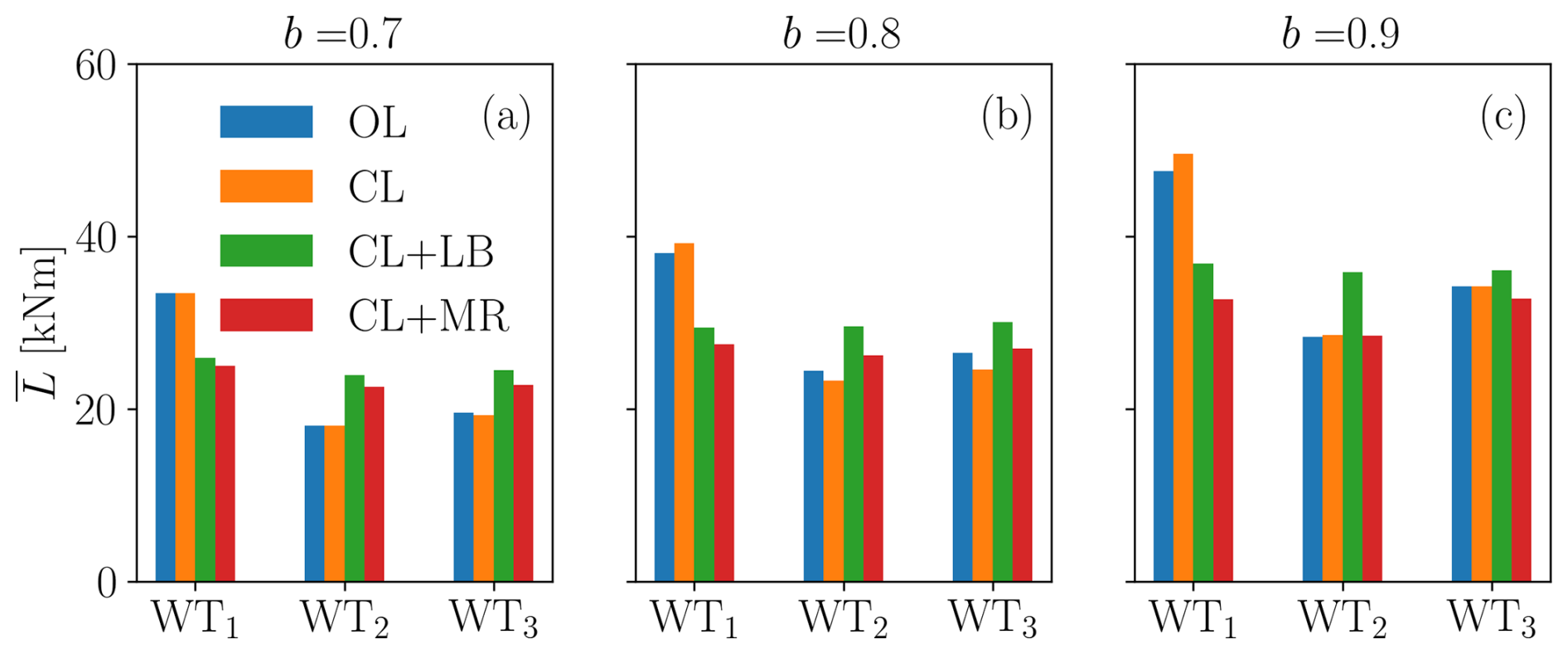
Figure 22 Mean tower-base fore–aft bending moment for the TSO demand levels b=0.7 (a), b=0.8 (b), and b=0.9 (c), for ψ=7.1° (50 % wake overlap).

The figures show that L increases with the TSO power demand level b. In all cases except CL+LB, WT₁ presents the largest load, while L is rather comparable for WT₂ and WT₃. CL+LB successfully balances L in the wind farm. It only fails to do so when b=0.9 for ψ=3.6° (75 % wake overlap), due to the persistent saturation of waked rotors. In this case, in fact, the controller is designed to prioritize power tracking over load balancing.

Interestingly, the proposed CL+MR also presents a rather balanced load distribution for ψ=7.1° (50 % wake overlap), but with slightly lower values than CL+LB. Conversely, for ψ=3.6° (75 % wake overlap), the loading on WT₃ grows along with b, due to the larger power share of this rotor compared to the other strategies.

Next, the effects on fatigue are analyzed by computing the damage equivalent loads (DELs) for the tower-base fore–aft bending moment using the rainflow counting algorithm (Downing and Socie, 1982). Simulations were performed with rigid wind turbine models, and hence, some dynamic effects are neglected. Nevertheless, this analysis still captures the effects generated by the different APC strategies on aerodynamically induced loads.

Figures 23 and 24 present the DELs of the three wind turbines in the array for ψ=3.6° (75 % wake overlap) and ψ=7.1° (50 % wake overlap), respectively.

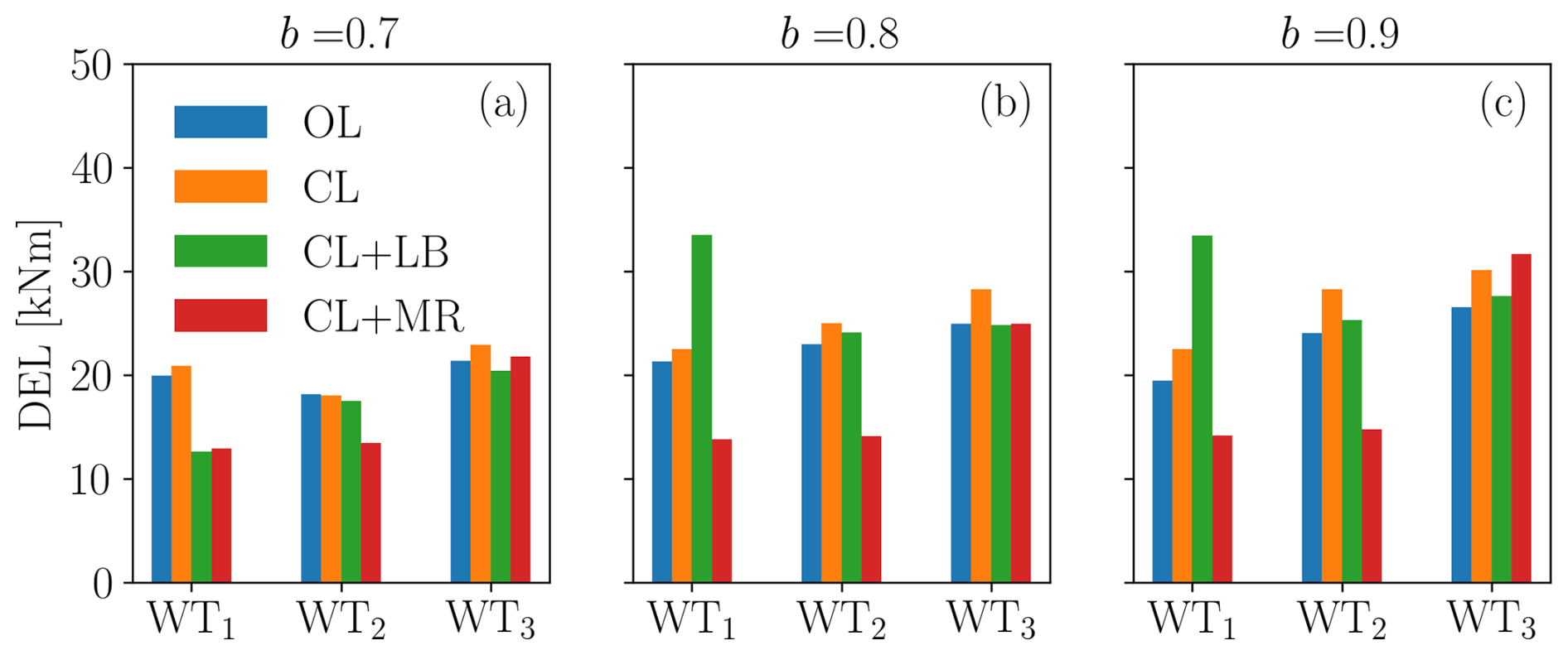
Figure 23 Tower-base fore–aft bending DELs for the cases b=0.7 (a), b=0.8 (b), and b=0.9 (c) for ψ=3.6° (75 % wake overlap).

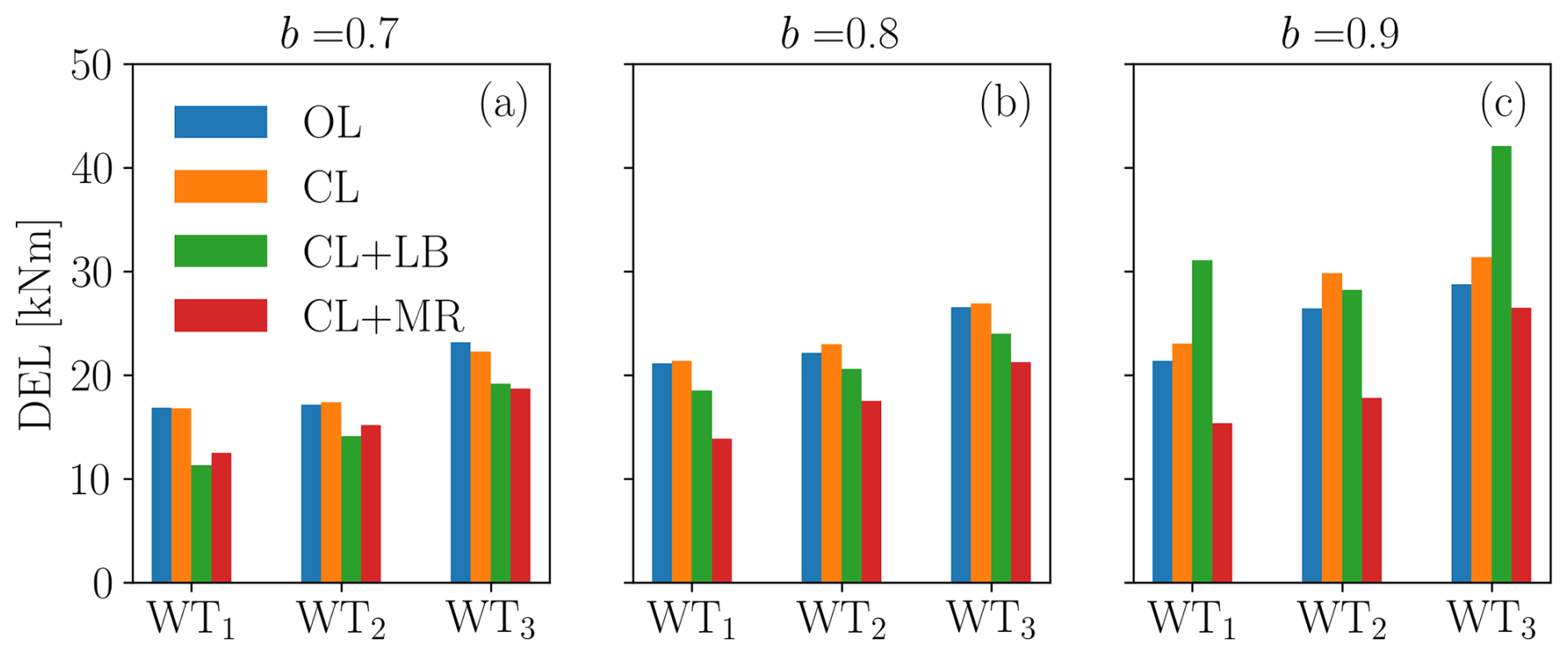
Figure 24 Tower-base fore–aft bending DELs for the cases b=0.7 (a), b=0.8 (b), and b=0.9 (c) for ψ=7.1° (50 % wake overlap).

Similarly to the average loading discussed earlier, DELs increase with TSO power demand b because of the higher loads that are involved. In general – and as expected – it appears that DELs grow as the turbines are more impinged by wakes. In fact, WT₃ is very often the most loaded turbine, possibly because of the relatively high turbulence associated with partial wake impingements.

There is, however, a notable exception for CL+LB (which is explicitly designed to ensure an equal balancing of the loads), where sometimes WT₁ is the most highly loaded machine. This is explained by the previous analyses (see Fig. 14), which showed that WT₁ is often the only turbine responsible for tracking the TSO signal, while the waked WT₂ and WT₃ operate in greedy mode. This points to the fact that load balancing by itself may not always be able to achieve the desired effect of an equal distribution of damage, defying its very design goal.

It is clear that the DELs in Figs. 23 and 24 could be biased by some unique events. These conditions can arise due to the high-amplitude cycles that occur, especially in correspondence with simultaneous saturation events. For this reason, no further conclusions are drawn from these plots. Rather, the fatigue analysis is repeated by binning the load time series according to the instantaneously required power, normalized by the available power of the wind farm, as done already in Sect. 3.4.1. In this case, multiple DELs are computed on continuous time segments of at least 45 s that belong to the same seed, and they are later summed together. DELs are computed in this way for each TSO demand scenario (b values), and they are then averaged. The results are shown in Figs. 25 and 26 for ψ=3.6° (75 % wake overlap) and ψ=7.1° (50 % wake overlap), respectively.

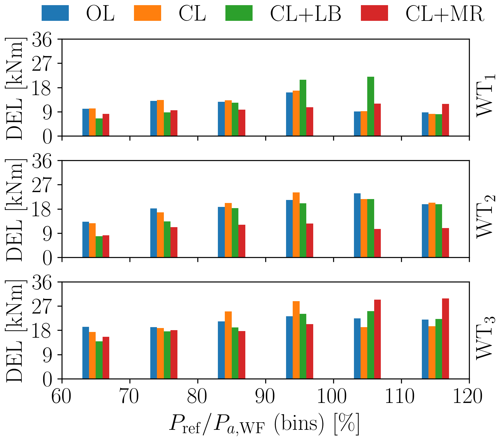
Figure 25 Tower-base fore–aft bending DELs for ψ=3.6° (75 % wake overlap). DELs are binned with the instantaneous available power, computed with the time series of greedy power and TSO power request. The values represent the mean over all the tested demands (b values). Only continuous time segments with a minimum duration of 45 s are considered.

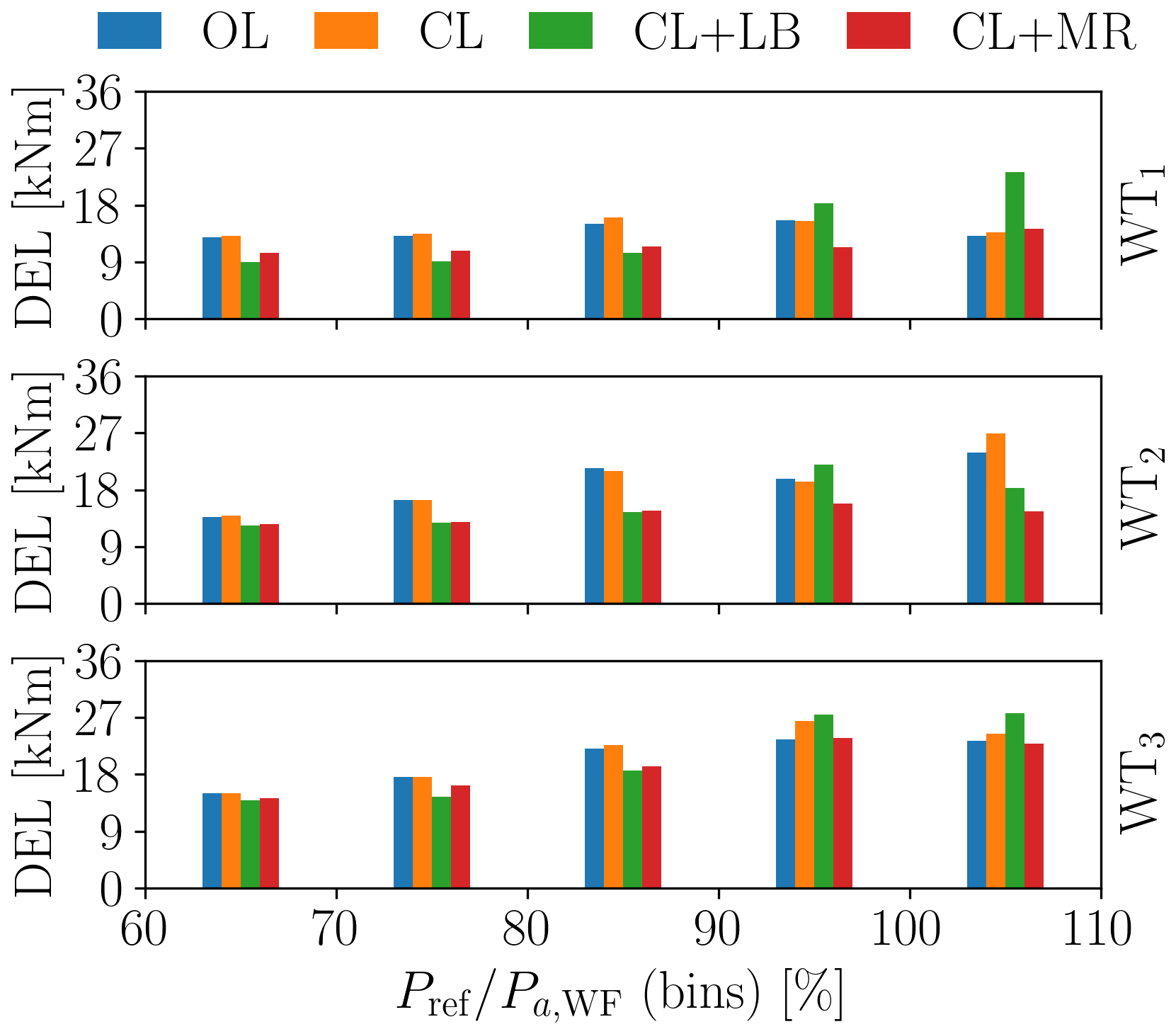
Figure 26 Tower-base fore–aft bending DELs for ψ=7.1° (50 % wake overlap). DELs are binned with the instantaneous available power, computed with the time series of greedy power and TSO power request. The values represent the mean over all the tested demands (b values). Only continuous time segments with a minimum duration of 45 s are considered.

These results allow for some further insight into the behavior of the various controllers. For all APCs, damage increases along with $P_{\mathrm{ref}}/P_{\mathrm{a},\mathrm{WF}}$. OL and CL do not present significant differences, as the power share distribution is similar. In these cases, the turbines operating in waked conditions are clearly more damaged than the upstream one. CL+LB works especially well for the simpler case of strong curtailments $P_{\mathrm{ref}}/P_{\mathrm{a},\mathrm{WF}}<\mathrm{80}\mathit{\%}$, with rather low DELs in accordance with Vali et al. (2019). Damage is also well distributed among the wind turbines but only in the less difficult cases.

Notably, the proposed CL+MR presents a relatively constant damage distribution, with improved performance especially in the more difficult cases for $P_{\mathrm{ref}}/P_{\mathrm{a},\mathrm{WF}}>\mathrm{80}\mathit{\%}$. Results also indicate a strong damage reduction on WT₁ and WT₂ for the larger rotor overlap condition (75 %, ψ=3.6°).

The previous analysis quantified fatigue damage but did not attribute it to specific dynamic sources. To distinguish the dominant sources of load unsteadiness, we categorize damage d based on the load cycle duration T obtained by rainflow counting, according to the following three bins:

• High frequency. $\mathrm{0}\mathrm{s}\le T\le \mathrm{5}$ s, generated by aerodynamic loads due to small turbulent eddies, rotational effects (1P, 3P harmonics), and the associated fast responses of the turbine and farm-level controllers;

• Medium frequency. $\mathrm{5}\mathrm{s}\le T\le \mathrm{30}$ s, associated with larger-scale flow eddies (the integral timescale of the inflow is approximately 11 s), including wake meandering, and the resulting control actions;

• Low frequency. $\mathrm{30}\mathrm{s}\le T\le \mathrm{20}$ min, caused by slower phenomena such as secondary grid frequency control (power tracking), long-period gusts, large-scale wake effects, and the resulting variations in power share (and hence loading).

Clearly, this definition of the bins is somewhat arbitrary but still enables a rough initial categorization of the driving phenomena. Since the simulations assume rigid wind turbine structures, aeroelastic dynamics are excluded from this analysis.

Figures 27 and 28 present the results of this binning, where we have considered the total damage deriving from the simulations with all the different TSO demand levels (b values). The damage that occurred in a specific cycle has been normalized with the damage of the baseline greedy control case (gray area in Figs. 12 and 13), so that the bars labeled “Greedy” sum up to 1.

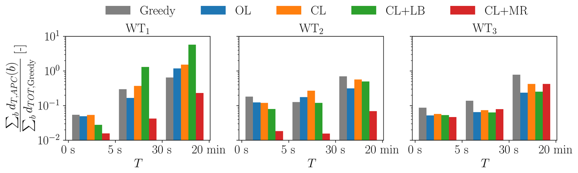
Figure 27 DELs of the tower-base fore–aft bending moment for ψ=3.6° (75 % wake overlap), binned by cycle duration T and normalized by the total damage of a baseline greedy control case in that bin.

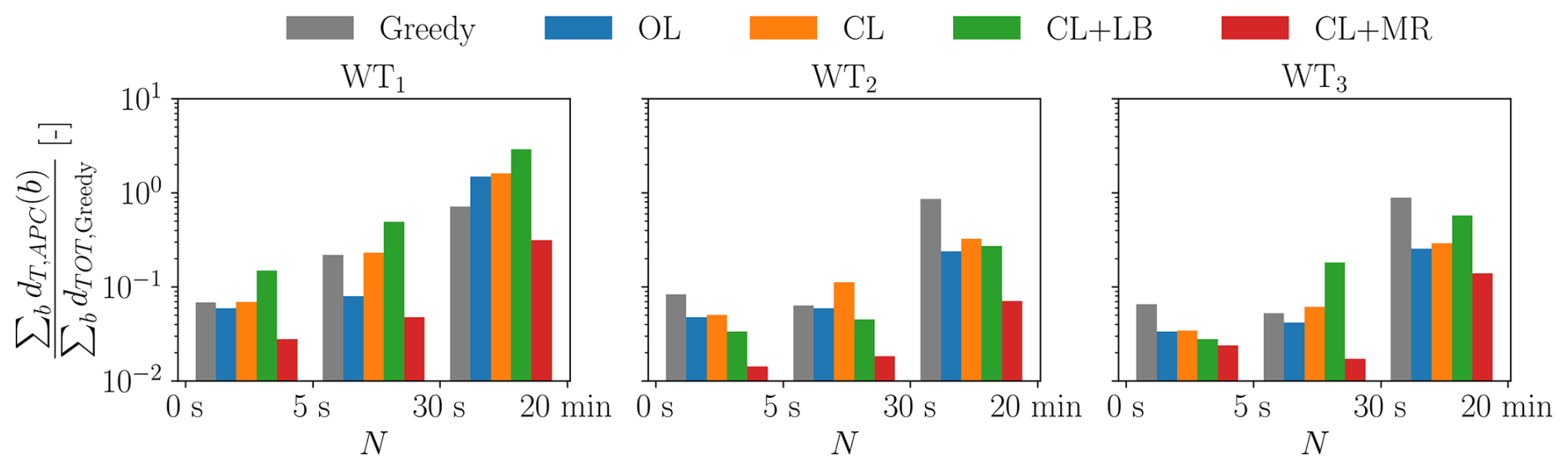
Figure 28 DELs of the tower-base fore–aft bending moment for ψ=7.1° (50 % wake overlap), binned by cycle duration T and normalized by the total damage of a baseline greedy control case in that bin.

Results indicate that the waked turbines WT₂ and WT₃ present more damage in the high-frequency range than WT₁, as a result of the small eddies that characterize wake turbulence.

The greedy case presents the highest damage in the low-frequency range for waked rotors (WT2 and WT3), likely due to strongly fluctuating inflows caused by wake impingement. All APC methods perform better than the greedy case because the low-frequency rotor dynamics are driven by the smooth reference power demand signal, so that large load fluctuations that would derive from wake turbulence are somehow mitigated.

As expected, closing the loop (CL) results in greater damage compared to operating in open loop (OL), especially in the medium frequency range, due to the extra turbine control activity that derives from the closed-loop correction. This is clearly visible in Fig. 13, where the local power oscillations of the various turbines are much larger when using CL than OL, especially for the higher TSO demand levels (b≥0.8). However, as already noted, these larger oscillations at the level of the turbines result in a much improved tracking of the power signal by the whole wind farm (cf. Figs. 13 and 18).

As already observed earlier, CL+LB in general performs rather poorly for WT₁ when compared to all other methods. This is due to the extra thrust-loading that results from the need to compensate for the saturations of WT₂ and WT₃. The effect of the added loading on damage is dramatic, due to the persistent saturations resulting from the CLD loop, as shown in Figs. 14 and 15.

The proposed CL+MR significantly outperforms all methods in the entire frequency spectrum for WT1 and WT2, due to the mitigation of wake impingement by wake steering, a generally reduced blade pitch actuation, and a particularly smooth power output made possible by the larger reserves, consistently with the time series shown in Figs. 12 and 13. This is true also for WT3 in the milder waking scenario (ψ=7.1°, 50 % wake overlap), thanks to wake steering that is able to clean its inflow. For the stronger waking case (ψ=3.6°, 75 % wake overlap), while the benefit on WT2 is dramatic, the performance for WT3 is similar to the other methods, probably due to the combined effects of two impinging wakes.

Overall, results indicate that low-frequency load cycles are responsible for the largest portion of damage. As shown in the time series of Figs. 12 and 13, low-frequency cycles of power (and therefore load) often coincide with saturations, especially when a compensation mechanism is in place, like in CL, CL+LB, and CL+MR. In fact, as a result of saturation, the compensating rotor has to track an additional power signal, which amplifies its control activity and increases fatigue. Furthermore, saturated rotors operate in greedy mode, which means that their loads are subjected to low-frequency variations deriving from the local inflow, which is often a waked one. This highlights once again the importance of the treatment and reduction of saturation events.

4 Conclusions and outlook

We have presented a new wind farm APC method to robustly track a reference power signal in turbulent wind conditions. The controller collectively operates the wind turbines to maximize the minimum local available power. This reserve can then be exploited for accurate power tracking, ensuring minimal insurgence of saturation events.

The algorithm combines one open loop and one closed loop, which operate at different time rates. A modified version of FLORIS was utilized to compute the wind turbine setpoints for the open-loop branch in a gradient-based optimization. The PI gains of the closed-loop branch were tuned with a digital twin that mimics the wind turbine dynamics and the propagation of wake effects.

The new methodology was tested on a small cluster of three wind turbines with persistent waking. We quantified the power reserve with a steady-state analysis and compared the new algorithm with a standard open-loop APC method. We observed that the new methodology is particularly effective at increasing power reserves when it can mitigate strong wake impingements.

In addition, the new approach was tested with unsteady LES-ALM simulations, showing an accurate power tracking performance, which was, in most cases, largely superior to the one provided by reference controllers representing the state of the art in APC. We have shown that this better accuracy is explained by the strong reduction of saturation events and the evenly spread power reserve, as measured by the mean collective blade pitch angle. We have binned the data according to the instantaneous available wind farm power to exclude biasing by isolated events.

Overall, the following observations should be highlighted:

• The power reserve of the wind turbines in a wind farm is significantly affected by the extent of wake impingement.

• The new methodology is very effective at creating additional reserves when the wind farm operates close to its maximum power capacity, because wake deficits are particularly strong in those conditions and the effectiveness of wake steering is maximum.

• Combining wake steering with induction control can improve wind farm performance by leveraging the strengths of both strategies. This can be particularly effective for optimizing objectives beyond power maximization, such as reducing structural loads, mitigating fatigue, and managing dynamic responses in general.

• Power tracking accuracy dramatically depends on the occurrence of saturation events. In this regard, the following should be noted:

  • –

    When one wind turbine saturates, it is extremely beneficial to redistribute its power tracking error in the form of an additional power demand to other turbines that are not saturated.

  • –

    The main hindrance to tracking accuracy is represented by conditions in which simultaneous saturations occur. These can trigger cascading effects of power redistribution or – in a worst case scenario – can push all wind turbines to operate in greedy mode even if the power demand of the wind farm is exceeded.

  • –

    When applying PI methods, it is extremely important to implement anti-windup procedures to hedge against saturations.

  • –

    In the presence of saturations, non-saturated turbines are called to compensate for the saturated ones, resulting in high-amplitude, low-frequency load cycles, which have a significant negative effect on fatigue.

• Saturations not only harm power tracking but also have significant effects on loads. In fact, load balancing (Vali et al., 2019) by itself fails to effectively balance loads in the presence of saturations. We have observed and reported here several instances where the proposed method, although lacking in the present implementation a dedicated load balancer, results in more uniform load distributions than CL+LB. This suggests that an improved version of the proposed CL+MR method might exhibit an even better performance if it included a load-balancing criterion. Beyond balancing, the proposed approach generally produced much reduced loadings on the turbines when compared to the alternative methods.

The main limitation of this work is the rather small duration of the LES-ALM simulations. Although in line with similar studies in the literature, this limited duration could have biased some results due to particular events occurring in the inflow time histories. To account for this, we performed greedy simulations to quantify the actual available power of the wind farm at every time instant. Another limitation of the unsteady results is the use of rigid wind turbine models in the simulations. If, on the one hand, this should not play a major role in the behavior of the far wakes (Salavatidezfouli et al., 2025), on the other hand, it somehow limits the conclusions that can be drawn from the analysis of fatigue.

Appendix A: Nomenclature

A	Ambient conditions
b	Shift of normalized power signal (power demand level)
CP	Power coefficient
CT	Thrust coefficient
c	Amplitude of normalized power signal
D	Rotor diameter
d	Damage
KI	Control gain (integral)
KP	Control gain (proportional)
L	Reference load signal (tower-base fore–aft bending moment)
$n_k^{\mathrm{AGC}}$	Normalized power demand perturbation
N	Number of turbines in a farm
P	Wind turbine power
PD	Wind turbine power demand
PR	Rated power
Pref	Reference power signal
pp	Cosine law exponent (yaw misalignment)
R	Rotor radius
r	Power reserve
s	Saturation
t	Time
T	Load cycle duration
U	Rotor-equivalent wind speed
U∞	Freestream wind speed at hub height
u	Control inputs
x	Cartesian coordinate
y	Cartesian coordinate
z	Cartesian coordinate
α	Power share setpoint
ΔL	Load-balancing error
ΔP	Power tracking error
ϵ	Curtailment
ηP	Power loss factor
γ	Rotor yaw angle
λ	Tip speed ratio
Ω	Rotor angular velocity
ΩR	Rated rotor angular velocity
ψ	Wind direction
ρ	Air density
θ	Blade pitch angle
AGC	Automatic generation control
APC	Active power control
CL	Closed loop
CLD	Coordinated load distribution
CL+LB	Closed loop with load balancing
CL+MR	Closed loop with maximum reserve
DEL	Damage equivalent load
FA	Fore–aft
FLORIS	FLOw Redirection and Induction in Steady State
OL	Open loop
PI	Proportional integral
RMS	Root mean square
SOWFA	Simulator fOr Wind Farm Applications
TI	Turbulence intensity
TSO	Transmission system operator
WF	Wind farm
WT	Wind turbine