From the center of wind pressure to loads on the wind turbine: a stochastic approach for the reconstruction of load signals

In the context of the wind industry, there is an increasing need for a more comprehensive understanding of atmospheric wind conditions. A particular emphasis is required concerning wind structures, which have not been thoroughly investigated in the prevailing standard guidelines. This necessity arises in light of the current trends toward larger, higher, and more flexible wind turbine designs. Of particular importance are the correlations between the yet-to-be-characterized atmospheric turbulent structures and the specific responses of the turbines. These correlations may be crucial in assessing load events relevant to new designs that were negligible for the earlier, smaller, and stiffer turbines. The center of wind pressure (CoWP) (Schubert et al., 2025) was recently introduced as a feature of a wind field that characterizes large-scale wind structures and, at the same time, correlates with the large-scale or low-frequency content of the bending moments at the main shaft of the wind turbines. In this paper, we comprehensively compare the CoWP and the bending moments in terms of their statistical properties and fatigue estimates, quantified by damage equivalent loads (DELs). Furthermore, a stochastic method for the reconstruction of synthetic CoWP signals is proposed. The strong correlation with the bending moments enables the proposed stochastic CoWP model to serve as a relatively simple surrogate and estimator of the large-scale dynamics of these loads, which is based solely on the properties of the inflow wind field. A notable advantage of the stochastic approach is its capability to reconstruct very long time series, required for evaluating loads over the operational lifetime of the turbine. For such lifetime estimations on wind turbines, it is necessary to combine the proposed model for large-scale dynamics with a corresponding model for small-scale features, site-specific wind conditions, and turbine-specific characteristics. The proposed stochastic model of the CoWP can be used not only for load assessment, but also for characterizing large-scale wind structures. The model offers an advanced description of wind phenomena, with the potential to be integrated as an extension of prevailing wind turbulence models.

1 Introduction

As part of the design and validation phase, numerical simulations are used to predict the loads on an operational wind turbine (WT). The objective of these simulations is to reproduce the interaction between the WT and the atmospheric turbulent wind. Given the inherently complex meso- to microscale nature of atmospheric phenomena, it is extremely difficult to attempt to incorporate the governing physical models into a unified description of the wind flow. Consequently, stochastic wind models, which involve numerous simplifications and assumptions of the atmosphere, are commonly employed for numerical simulations of WTs. Common examples are the Kaimal (Kaimal et al., 1972), von Kármán (Von Kármán, 1948), and Mann (Mann, 1998) wind models. The International Electrotechnical Commission (IEC) (IEC, 2019) has proposed these models as standard atmospheric turbulence representations for numerical WT simulations. It should be noted that these models are based on low-order statistical features of the wind fields, such as power spectra and correlations. However, they do not yet explicitly resolve the turbulent eddies, i.e., the spatial characteristics of the turbulent flow structures. For the spatial coherence of turbulence, an exponential decay with distance is assumed. The IEC standard also considers some extreme operating conditions (EOCs), encompassing peak wind speeds, gusts, and sudden changes in wind direction. These non-realistic extreme wind structures are conceived as homogeneous in space (i.e., uniform over the entire rotor area), with a return period of 50 years.

Recent advancements in WT design show a persistent trend towards increasing dimensions, including higher heights and larger rotor diameters. Accordingly, certain structural properties are significantly modified within the designs of larger WTs. Specifically, a higher degree of flexibility is characteristic of larger and slimmer rotor blades. This may raise concerns about the validity of the assumptions or the omission of specific turbulent structures within the aforementioned standard wind models currently used by the WT industry. The increased scale of WTs suggests that certain wind characteristics, which were previously negligible or unimportant for smaller and more rigid WTs, may be significant considerations within the aerodynamic interactions of state-of-the-art WT designs. Of particular interest are the spatial properties of the atmospheric wind structures. Rotor diameters that exceed 200 m may exhibit sensitivity to the spatial characteristics of wind phenomena, such as wind gusts.

The necessity for an extended characterization of atmospheric turbulent wind beyond the parameters currently outlined in the IEC standard guidelines is supported by the repeated measurement of unexpected loads in operational WTs. According to manufacturers and operators of WTs, numerical simulations of the specific WTs and the standard IEC wind modeling assumptions do not adequately reflect certain load events that may be important for the structural integrity of the machines in operation. Consequently, it is imperative to establish a correlation between the extended features of the atmospheric wind and the measured unexpected effects on the operating WTs. Examples of such extended characteristics of atmospheric turbulence include small-scale intermittency (Boettcher et al., 2003; Morales et al., 2012), low-level jets (Gutierrez et al., 2016), particular coherent vortices (Abraham and Hong, 2022), fractal turbulent–non-turbulent interfaces (Neuhaus et al., 2024), wind ramp events (Gallego-Castillo et al., 2015), and periods of constant wind speed (Moreno et al., 2025).

A general requirement within the wind industry is to simplify the complexity of WT representations in turbulent wind environments to allow practical implementation and minimize computational costs. As stipulated in the standard guidelines (IEC, 2019), numerical simulations of a wide range of operational scenarios are required for the validation of WT designs. Consequently, optimizing the computational time and power while ensuring satisfactory accuracy of the estimations of the responses of the WT is imperative. Some approaches have been proposed to reduce the complexity of the interaction between the wind and the WT. Examples of methods based on a given wind field include a modified actuator sector model for WT simulations (Mohammadi et al., 2024) and the calculation of extended equivalent wind speeds over the rotor area (Choukulkar et al., 2016). Conversely, techniques are employed to extract characteristics of the incoming flow field from load measurements at the WT, such as blade-load-based estimators (Coquelet et al., 2024). Furthermore, due to the limitations in computational power, the loads on the WT are typically estimated over short intervals, e.g., 10 min. Consequently, numerical techniques have been proposed for extrapolating the loads estimated from such short timescales to lifetime scenarios containing fatigue damage and extreme load events (Zhang and Dimitrov, 2023; Qingshan et al., 2022).

The virtual center of wind pressure (CoWP) has recently been introduced as a feature of a given wind field that is either measured or modeled (Schubert et al., 2025). The CoWP characterizes large-scale wind structures occurring over the plane perpendicular to the main direction of the wind, i.e., the rotor plane, when considering a WT. Most interestingly, the CoWP is directly correlated to the low-frequency content of the bending moments at the main shaft of the WT. Consequently, the CoWP not only facilitates the characterization of extended wind structures, i.e., beyond the IEC standard, but also proposes a simplified and expeditious method for assessing the particular characteristics of the WT loads.

In this article, we first aim to perform a comprehensive comparison between the CoWP, calculated from the wind fields, and the bending moments at the shaft of the WT, calculated using blade element momentum (BEM) numerical simulations. The statistical characteristics of the signals and their damage equivalent loads (DELs) are investigated. Second, based on the correlation between the large-scale structures of both the CoWP and the bending moments, we propose a stochastic method to derive the dynamics of the former, which are subsequently the basis for generating surrogate signals of the latter. The statistics of the surrogate data demonstrate a high degree of comparability to those of the original CoWP from the wind fields, as well as to the low-frequency content of the BEM-simulated bending moments. A notable advantage of the stochastic reconstruction is its capacity to generate very long time series. The availability of such extensive data is essential for assessing lifetime load events without the necessity of numerical extrapolation techniques.

Our model thus offers a twofold approach. On the one hand, it facilitates the characterization and modeling of large-scale wind structures. The wind energy sector is in urgent need of a comprehensive description of these large-scale structures, as standard wind models are likely to oversimplify them. Modern large wind turbines are particularly vulnerable to this oversimplification. On the other hand, our stochastic model allows the estimation and extrapolation of specific characteristics of the bending moments at the main shaft while bridging these responses of the WT with structures of the inflow wind field. In its current state, the method is limited to the modeling of the dynamics of the low-frequency components of the bending moments. However, when combined with a description of the high-frequency components, a validated rescaling procedure, and the characterization of the site-specific wind conditions, this approach enables a novel method for a fast assessment of the lifetime loads in WTs. In a preliminary investigation (Moreno et al., 2024), the stochastic method for reconstructing the time series of loads based on the dynamics of the CoWP from IEC-standard-modeled wind fields was introduced. The present paper extends the stochastic approach to wind data from atmospheric measurements.

The paper is structured as follows. Section 2 presents the relevant definitions that are discussed in the paper. Section 3 describes the wind data that are investigated. The analysis of the reconstructed data from IEC-standard-modeled wind fields and atmospherically measured data is presented in Sect. 4. Finally, the conclusions and outlook of our investigation are stated in Sect. 5.

2 Definitions

2.1 Center of wind pressure

The virtual center of wind pressure (CoWP) is defined by Schubert et al. (2025) as the two-dimensional position in the plane of the rotor at which a point-wise thrust force F_T acts and induces the bending moments T. This position is specified with respect to a reference point, e.g., the main shaft of a WT. The moments are estimated as $\mathbf{T}=\mathrm{CoWP}\times {\mathit{F}}_{\mathrm{T}}$. Figure 1 illustrates the concept of the CoWP, introduced as a characteristic of a given wind field $\mathbf{u}(y,z,t)$.

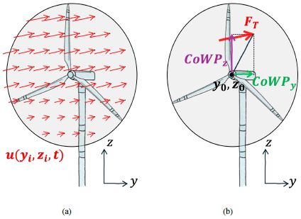
Figure 1 Schematic illustration of (a) the wind field $\mathbf{u}(y,z,t)$ over the area of a rotor disk and (b) the resulting two-dimensional CoWP calculated from the wind field.

In the following, a brief derivation of the concept of the CoWP is presented. Let us consider a wind field $\mathbf{u}(y_i,z_i,t)$ defined over a discretized grid with 𝒩 points on the rotor plane, i.e., the y–z plane, perpendicular to the main direction of the flow. Then, the normal thrust force F_T acting over the rotor area 𝒜 at the y–z plane is calculated as

$$\begin{array}{}\text{(1)}& F_T\left(t\right)={\displaystyle \frac{\mathrm{1}}{\mathrm{2}}}\sum _{i=\mathrm{1}}^{\mathcal{N}}{\mathit{\rho }}_{\mathrm{air}}{C}_{\mathrm{T}}{u}^{\mathrm{2}}(y_i,z_i,t)\mathrm{\Delta }{\mathcal{A}}_i,\end{array}$$

where u is the longitudinal component of the wind perpendicular to the y–z plane, ρ_air is the density of air, C_T is the thrust coefficient of the rotor, and Δ𝒜_i is the discretized section of the rotor area 𝒜. Now, the bending moments T due to the normal thrust force can be calculated as

$$\begin{array}{}\text{(2)}& \mathbf{T}\left(t\right)=\stackrel{\mathrm{̃}}{\mathit{r}}\left(t\right)\times F_T\left(t\right),\end{array}$$

where $\stackrel{\mathrm{̃}}{\mathit{r}}$ is the distance between the acting location of F_T to the reference point. Considering the main shaft, i.e., the center of the rotor disk (y₀, z₀), as the reference point, the yaw T_yaw and tilt T_tilt moments at the main shaft are estimated as

$$\begin{array}{}\text{(3)}& \begin{array}{rl}& T_{\mathrm{yaw}}\left(t\right)={\displaystyle \frac{\mathrm{1}}{\mathrm{2}}}\sum _{i=\mathrm{1}}^{\mathcal{N}}{\stackrel{\mathrm{̃}}{y}}_i{\mathit{\rho }}_{\mathrm{air}}{C}_{\mathrm{T}}{u}^{\mathrm{2}}(y_i,z_i,t)\mathrm{\Delta }{\mathcal{A}}_i\\ & T_{\mathrm{tilt}}\left(t\right)={\displaystyle \frac{\mathrm{1}}{\mathrm{2}}}\sum _{i=\mathrm{1}}^{\mathcal{N}}{\stackrel{\mathrm{̃}}{z}}_i{\mathit{\rho }}_{\mathrm{air}}{C}_{\mathrm{T}}{u}^{\mathrm{2}}(y_i,z_i,t)\mathrm{\Delta }{\mathcal{A}}_i,\end{array}\end{array}$$

where $\stackrel{\mathrm{̃}}{y}$ and $\stackrel{\mathrm{̃}}{z}$ are the horizontal and vertical distances, respectively, of each location i to the reference point so that ${\stackrel{\mathrm{̃}}{y}}_i=y_i-y_{\mathrm{0}}$ and ${\stackrel{\mathrm{̃}}{z}}_i=z_i-z_{\mathrm{0}}$. Assuming $\frac{\mathrm{1}}{\mathrm{2}}{\mathit{\rho }}_{\mathrm{air}}{C}_{\mathrm{T}}$ to be constant, the two CoWP components are defined as the fraction of the moments (yaw and tilt) and the normal thrust force, resulting in

$$\begin{array}{}\text{(4)}& \begin{array}{rl}& {\mathrm{CoWP}}_y\left(t\right)={\displaystyle \frac{{\sum }_{i=\mathrm{1}}^{\mathcal{N}}{\stackrel{\mathrm{̃}}{y}}_i{u}^{\mathrm{2}}(y_i,z_i,t)\mathrm{\Delta }{\mathcal{A}}_i}{{\sum }_{i=\mathrm{1}}^{\text{n}}{u}^{\mathrm{2}}(y_i,z_i,t)\mathrm{\Delta }{\mathcal{A}}_i}}\\ & {\mathrm{CoWP}}_z\left(t\right)={\displaystyle \frac{{\sum }_{i=\mathrm{1}}^{\mathcal{N}}{\stackrel{\mathrm{̃}}{z}}_i{u}^{\mathrm{2}}(y_i,z_i,t)\mathrm{\Delta }{\mathcal{A}}_i}{{\sum }_{i=\mathrm{1}}^{\mathcal{N}}{u}^{\mathrm{2}}(y_i,z_i,t)\mathrm{\Delta }{\mathcal{A}}_i}}.\end{array}\end{array}$$

The CoWP is calculated solely by wind field data, comprehensively representing specific wind structures, whether modeled or measured. Furthermore, the area 𝒜, used to compute the CoWP, can be adapted to investigate diverse sizes and domains within fields, e.g., one-dimensional dynamics, when measuring atmospheric data with vertically aligned devices in a met mast or different WT rotor sizes from numerically modeled wind fields.

2.2 Damage equivalent load

The damage equivalent load (DEL) is the method recommended by the standard IEC (2019) for performing fatigue assessments and damage calculation analyses of the mechanical elements of the WT. In essence, the DEL represents a fixed-amplitude and fixed-frequency load, calculated from a load signal encompassing a range of frequencies and amplitudes. Based on Miner's rule (Miner, 1945) and the rainflow counting method (Matsuishi and Endo, 1968; Downing and Socie, 1982), the DEL is calculated over a period T as

$$\begin{array}{}\text{(5)}& \text{DEL}={\left({\displaystyle \frac{{\sum }_{i=\mathrm{1}}^n{n}_i{s}_i^m}{N_f}}\right)}_T^{m^{-\mathrm{1}}},\end{array}$$

where n_i is the number of cycles with amplitude s_i, and N_f is a reference number of cycles. The Wöhler exponent m is characteristic of the material and is extracted from the so-called S–N curves (Basquin, 1910). Note that, according to Eq. (5), the contribution of the amplitudes s_i to the DEL is determined by the exponent m. The larger the value of m, the stronger the dominance of larger amplitudes s_i within the calculation of the DEL. More details about the estimation and assumptions of the DEL can be found in Sutherland (1999). This study uses the DEL to evaluate the effect on the bending moments at the main shaft induced by the wind structures characterized by the CoWP.

2.3 The stochastic Langevin model

The CoWP, calculated from a given wind field, can be characterized in terms of its statistical properties and dynamical behavior. Since the CoWP signals are noisy and irregular, we introduce the Langevin model as a stochastic approach to characterize the dynamics. The range of applications of the Langevin method is extensive, encompassing domains as diverse as medical signals, e.g., human balance (Rinn et al., 2016b; Bosek et al., 2004) or brain activity (Costa et al., 2016), financial markets (Friedrich et al., 2000), and cone penetration signals for stratigraphy (Lin et al., 2022).

Assuming a one-dimensional stochastic process X(t), the general differential Langevin equation,

$$\begin{array}{}\text{(6)}& {\displaystyle \frac{\mathrm{d}}{\mathrm{d}t}}X=D^{\left(\mathrm{1}\right)}(X,t)+\sqrt{D^{\left(\mathrm{2}\right)}(X,t)}\mathrm{\Gamma }\left(t\right),\end{array}$$

describes the temporal derivative $\frac{\mathrm{d}X}{\mathrm{d}t}$ as the sum of two contributions: a deterministic part driven by the drift coefficient D⁽¹⁾ and a stochastic component driven by the diffusion coefficient D⁽²⁾ and weighted by a stochastic force Γ(t) (Lemons and Gythiel, 1997; Risken, 1996), where Γ(t) is Gaussian noise with a mean of 0 and a δ correlation; i.e., 〈Γ(t)〉=0 and $\langle \mathrm{\Gamma }\left(t\right)\mathrm{\Gamma }(t-t^{\prime })\rangle =\mathrm{2}\mathit{\delta }(t-t^{\prime })$. The angular brackets 〈…〉 denote the temporal average.

The Langevin method, introduced by Friedrich and Peinke (1997) and Siegert et al. (1998), proposes an approach to derive the coefficients D^(k) from time series X^′(t). This is achieved by calculating the derivative of the conditional moments $M^{\left(k\right)}(X,t,\mathit{\tau })$ for the state $X=X^{\prime }\left(t\right)$ of the system as

$$\begin{array}{}\text{(7)}& D^{\left(k\right)}(X,t)=\underset{\mathit{\tau }\to \mathrm{0}}{lim}{\displaystyle \frac{\mathrm{1}}{\mathit{\tau }}}{M}^{\left(k\right)}(X,t,\mathit{\tau })\end{array}$$

for $k=[\mathrm{1},\mathrm{2}]$, where τ is a small-enough time step. The conditional moment $M^{\left(k\right)}(X,t,\mathit{\tau })$ is calculated by averaging the kth power of the increments, $X^{\prime }(t+\mathit{\tau })-X$, as

$$\begin{array}{}\text{(8)}& M^{\left(k\right)}(X,t,\mathit{\tau })={\displaystyle \frac{\mathrm{1}}{k\mathrm{!}}}\langle {\left[X^{\prime }(t+\mathit{\tau })-X\right]}^k{\mathrm{|}}_{X^{\prime }\left(t\right)=X}\rangle .\end{array}$$

Now, for a two-dimensional process $\mathbf{X}\left(\mathbf{t}\right)=\mathit{\left\{}{X}_{\mathrm{1}}\right(t),X_{\mathrm{2}}(t\left)\mathit{\right\}}$, the Langevin equation has the form

$$\begin{array}{}\text{(9)}& {\displaystyle \frac{\mathrm{d}}{\mathrm{d}t}}\left[\begin{array}{c}{X}_{\mathrm{1}}\\ X_{\mathrm{2}}\end{array}\right]=\left[\begin{array}{c}{D}_{\mathrm{1}}^{\left(\mathrm{1}\right)}(\mathbf{X},t)\\ D_{\mathrm{2}}^{\left(\mathrm{1}\right)}(\mathbf{X},t)\end{array}\right]+\left[\begin{array}{cc}{D}_{\mathrm{11}}^{\left(\mathrm{2}\right)}(\mathbf{X},t)& D_{\mathrm{12}}^{\left(\mathrm{2}\right)}(\mathbf{X},t)\\ D_{\mathrm{21}}^{\left(\mathrm{2}\right)}(\mathbf{X},t)& D_{\mathrm{22}}^{\left(\mathrm{2}\right)}(\mathbf{X},t)\end{array}\right]\left[\begin{array}{c}{\mathrm{\Gamma }}_{\mathrm{1}}\left(t\right)\\ {\mathrm{\Gamma }}_{\mathrm{2}}\left(t\right)\end{array}\right],\end{array}$$

with the diffusion coefficients $D_{\mathrm{12}}^{\left(\mathrm{2}\right)}$ and $D_{\mathrm{21}}^{\left(\mathrm{2}\right)}$,

$$\begin{array}{}\text{(10)}& \begin{array}{rl}{D}_{\mathrm{12}}^{\left(\mathrm{2}\right)}& (\mathbf{X},t)=D_{\mathrm{21}}^{\left(\mathrm{2}\right)}(\mathbf{X},t)={\displaystyle \frac{\mathrm{1}}{\mathrm{2}}}\underset{\mathit{\tau }\to \mathrm{0}}{lim}{\displaystyle \frac{\mathrm{1}}{\mathit{\tau }}}\langle \left[X_{\mathrm{1}}^{\prime }(t+\mathit{\tau })-X_{\mathrm{1}}\right]\\ & \left[X_{\mathrm{2}}^{\prime }(t+\mathit{\tau })-X_{\mathrm{2}}\right]{\mathrm{|}}_{X_{\mathrm{1}}=X_{\mathrm{1}}^{\prime }\left(t\right),X_{\mathrm{2}}=X_{\mathrm{2}}^{\prime }\left(t\right)}\rangle .\end{array}\end{array}$$

Once the coefficients D^(1,2) are known, the method can be reversed. Then, time series X(t) can be generated via the stochastic integration of Eq. (9). The application of the Langevin approach for the stochastic reconstruction of the time series of the two-dimensional CoWP is discussed in the next section. Further developments of and details on the Langevin model can be found in Friedrich et al. (2011), Reinke et al. (2015), Rinn et al. (2016a), and Tabar (2019).

2.4 Stochastic model for CoWP and WT loads

In Fig. 2, we schematically show our proposed stochastic method in the context of load estimation of the low-frequency contribution of the bending moments at the main shaft of a WT. Starting from either a modeled or a measured wind field $\mathbf{u}(y,z,t)$, the CoWP is calculated according to Eq. (4) (going in the upward direction in Fig. 2). Then, the stochastic Langevin approach is used to derive the coefficients D^(1,2) from the CoWP signals. Based on the extracted coefficients D^(1,2), the stochastic reconstruction of signals of the low-frequency bending moments at the main shaft can be achieved. The strength of this approach lies in its ability, based on the Langevin stochastic differential equation, to generate a time series of any length while preserving the statistical properties of the original CoWP data from the wind field data. This feature is particularly advantageous, as lifetime load assessments of a WT require large amounts of computationally expensive data or numerical extrapolation techniques. However, the implementation of the stochastic method for lifetime load assessment in engineering applications (i.e., including both the high- and the low-frequency components of the loads) is constrained in its application. To ensure a comprehensive lifetime model, it is necessary to incorporate additional elements. A turbine-specific transfer function for rescaling the magnitudes of the loads is required. A complementary model for the high-frequency components of the loads must be integrated. Finally, the occurrence of the loads must be weighted by the distribution of the mean wind speed at the location of the WT (e.g., annual Weibull distribution).

The current standard procedure for load assessment in the wind industry is shown in the downward direction from the wind field $\mathbf{u}(y,z,t)$ in Fig. 2. In brief, the response of a WT to a specific inflow wind field is investigated via a BEM simulation, with a typical length of 10 min. The time series of the loads are obtained from several 10 min random realizations that account for different wind conditions. Thus, the assessment of all required wind situations is computationally very demanding. After the aggregation of 10 min BEM simulations, extrapolation methods are applied to account for extreme load events and damage calculation during the lifetime of the WT (Zhang and Dimitrov, 2023; Qingshan et al., 2022). Compared to the standard approach, our proposed model is computationally very efficient and thus fast. The lowest path in Fig. 2, depicted by dashed lines, shows the potential use of operational wind and load measurements for validation and optimization processes.

As a side comment, the description of the dynamics of the CoWP, e.g., via the derivation of D^(1,2), provides a comprehensive characterization of the large-scale structures in the wind field, which can be further investigated. For instance, it can be used to estimate the accuracy of modeled wind data compared to atmospheric measurements, or it can be included as a parameterization into extensive descriptions of the turbulent wind, such as the IEC standard models or other surrogate models for wind field reconstruction (Yassin et al., 2023; Friedrich et al., 2022; Rinker, 2018).

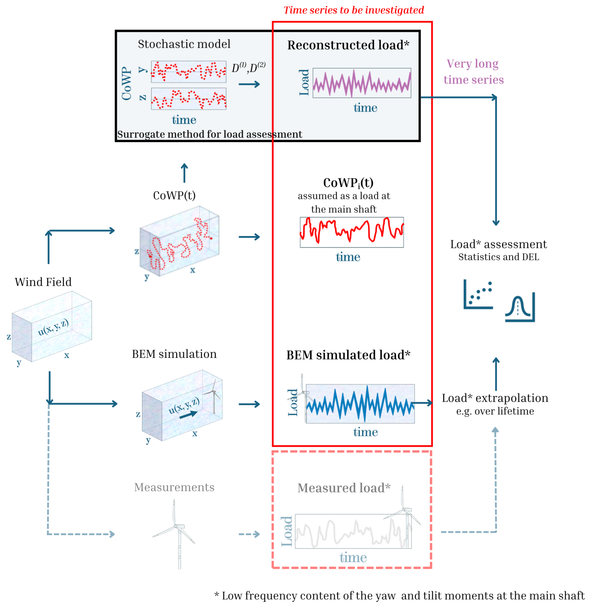
Figure 2 Diagram of the stochastic surrogate method for the assessment of the low-frequency content of the bending moments at the main shaft given a wind field $\mathbf{u}(x,y,z)$. The proposed method goes upwards from the wind field in the figure. For comparison, the path in the downward direction shows the standard procedure for load estimations specified by the IEC standard guideline. The solid red box contains the three data sets to be compared in the following sections. The dashed lines at the lowest part of the figure represent operational measured data to be potentially included in an extended comparison.

The solid red box in Fig. 2 schematically shows the three data sets that are compared and discussed in the following sections of this paper. From the bottom to the top are the following:

• a.

  the bending moments at the main shaft calculated by BEM simulations

• b.

  the CoWP calculated from the modeled or measured wind fields (see Sect. 3)

• c.

  the time series generated via the stochastic reconstruction.

Again, the dashed line shows a potential use of operational load data to be included in the comparison.

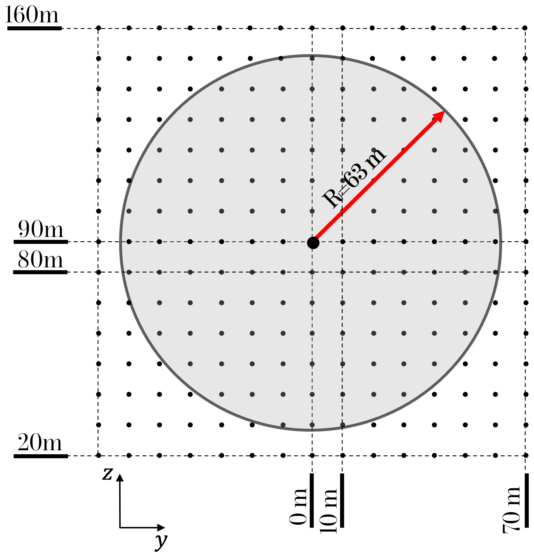
Figure 3 Schematic representation of the Kaimal spatial grid and the 5 MW NREL rotor. The black points depict the discrete locations of the spatial grid with $\mathrm{\Delta }y=\mathrm{\Delta }z=\mathrm{10}\mathrm{m}$. The hub of the model WT is located at the center point of the grid at y=0 and z=90 m.

3 Wind data: IEC standard fields and atmospheric measurements

We aim to characterize and model the CoWP from two wind data sets:

• i.

  IEC standard Kaimal data. Synthetic wind fields are generated with the Kaimal model (Kaimal et al., 1972) proposed by the IEC standard (IEC, 2019). The fields are defined in a 130 m × 130 m spatial grid with a separation $\mathrm{\Delta }y=\mathrm{\Delta }z=\mathrm{10}\mathrm{m}$ and are centered at y=0 and z=90 m. The grid points are shown schematically by the small black dots in Fig. 3. The circular gray area depicts the scaled rotor of the 5 MW NREL turbine (Jonkman et al., 2009) with hub height at 90 m and a rotor diameter of 126 m. The mean wind speed $\stackrel{\mathrm{‾}}{u}=\mathrm{7}$ m s⁻¹ and turbulence intensity TI=7 % of the non-shear wind fields are defined at the location of the hub. The BEM simulations of the 5 MW NREL turbine are performed in OpenFAST (Jonkman et al., 2025). A total of 4.7×10⁴ s of simulated time is investigated. The TurbSim package (Jonkman, 2016) was used to generate the Kaimal fields. The implementation in TurbSim of the Kaimal spectrum for the longitudinal component u of the wind follows

  $$\begin{array}{}\text{(11)}& E_u\left(f\right)={\displaystyle \frac{\mathrm{4}{\mathit{\sigma }}_u^{\mathrm{2}}{L}_u/{\stackrel{\mathrm{‾}}{u}}_H}{(\mathrm{1}+\mathrm{6}f{L}_u/{\stackrel{\mathrm{‾}}{u}}_{\mathrm{H}}{)}^{\mathrm{5}/\mathrm{3}}}},\end{array}$$

  where σ_u is the standard deviation of u, ${\stackrel{\mathrm{‾}}{u}}_{\mathrm{H}}$ is the mean at hub height, and f is the frequency. The integral scale L_u is defined as L_u=8.10Λ_u, with Λ_u being the turbulence scale. Λ_u is calculated as ${\mathrm{\Lambda }}_u=\mathrm{0.7}\left(\min \mathit{\right\{}\mathrm{30}\mathrm{m},H_{\mathrm{H}}\mathit{\left\}}\right)$, where H_H is the hub height. In conjunction with the Kaimal spectra, an exponential coherence model is assumed to describe the spatial correlation of the longitudinal component u. The coherence scale parameter L_c for the coherence model (IEC, 2019) is assumed as $L_{\mathrm{c}}=L_u=\mathrm{8.10}{\mathrm{\Lambda }}_u$.

• ii.

  Atmospheric GROWIAN data. The measurement campaign was conducted in Germany between 1984 and 1987. The horizontal wind speed was measured with a frequency of 2.5 Hz by 16 propeller anemometers arranged in two met masts, covering an area of 76 m × 100 m. Details of the GROWIAN data are found in Körber et al. (1988) and Günther and Hennemuth (1998). The blue circles in Fig. 4 illustrate a schematic representation of the measurement arrangement. The GROWIAN data have been conditioned by the mean wind speed $\mathrm{8.5}\le \stackrel{\mathrm{‾}}{u}<\mathrm{11.5}$ m s⁻¹, turbulence intensity $\mathrm{6}\le \text{TI}<\mathrm{12}\mathit{\%}$, and shear exponent $\mathrm{0}\le q<\mathrm{0.06}$. The characteristics $\stackrel{\mathrm{‾}}{u}$, TI, and q are calculated over 10 min periods at the location with coordinates $y=-\mathrm{14}$ and z=100 m. To guarantee an undisturbed flow, the wind direction over the 10 min periods remains within a 100° range with respect to the location of the two met masts (i.e., main direction of the flow). After the conditioning, 18 blocks of 10 min intervals or 1.08×10⁴ s is considered for the analysis.

  In order to perform BEM simulations of a realistic WT, a rescaling of the GROWIAN data is needed. The rescaled GROWIAN fields are defined on a stretched grid of 152 m × 150 m. The stretching is performed by increasing the distance between neighboring points of the original grid by a factor of 1.5 in the vertical direction and a factor of 2 in the horizontal direction. The green circles in Fig. 4 illustrate the rescaled GROWIAN spatial arrangement, centered at y=0 and z=125 m. The wind speed measurements at the 16 original locations have not been modified. The four grid points at the corners of the stretched grid are filled with the data from the next neighboring grid point at the same height. For example, the wind speed at the corner point (−76, 50 m) is assumed to be identical to the point at (−76, 25 m). The gray area in Fig. 4 depicts the WT model that is simulated. The hub of the WT is located at 125 m, and the rotor diameter is 149 m. The BEM simulations are performed with the alaska/Wind aero-elastic-servo simulator (ICM, 2023; Zierath et al., 2016), developed at the Institute of Mechatronics in Chemnitz, Germany. The multi-body alaska/Wind model incorporates several coupled sub-models: the foundation, the tower, the nacelle, the yaw drive, the pitch drive, the rotor, the drive train, the generator, and the controller. A Beddoes–Leishman-type dynamic model and a flexible wake model consider the unsteady airfoil aerodynamics and the wake effects, respectively. Among the specified degrees of freedom are the radial degree in the drive train for torsional effects of the gearbox; the nodding degree in the yaw drive; and the side-to-side, fore–aft, and torsional motions of the tower. These considerations regarding the modeling assumptions of the simulations follow the simulations in Schubert et al. (2025).

It is important to note that the simplified wind field rescaling in this study results in some degree of distortion to the spatial correlations of the original GROWIAN data. The introduced distortion, under the assumption of self-similarity of turbulence, is of minor significance, as our primary utilization of the GROWIAN data is to develop realistic, large-scale structures of the turbulent atmospheric boundary layer. Large-scale wind structures (e.g., of the size of the rotor diameter) are not present in other standard numerical wind fields. They will become important for the CoWP and the loads, as demonstrated in the following.

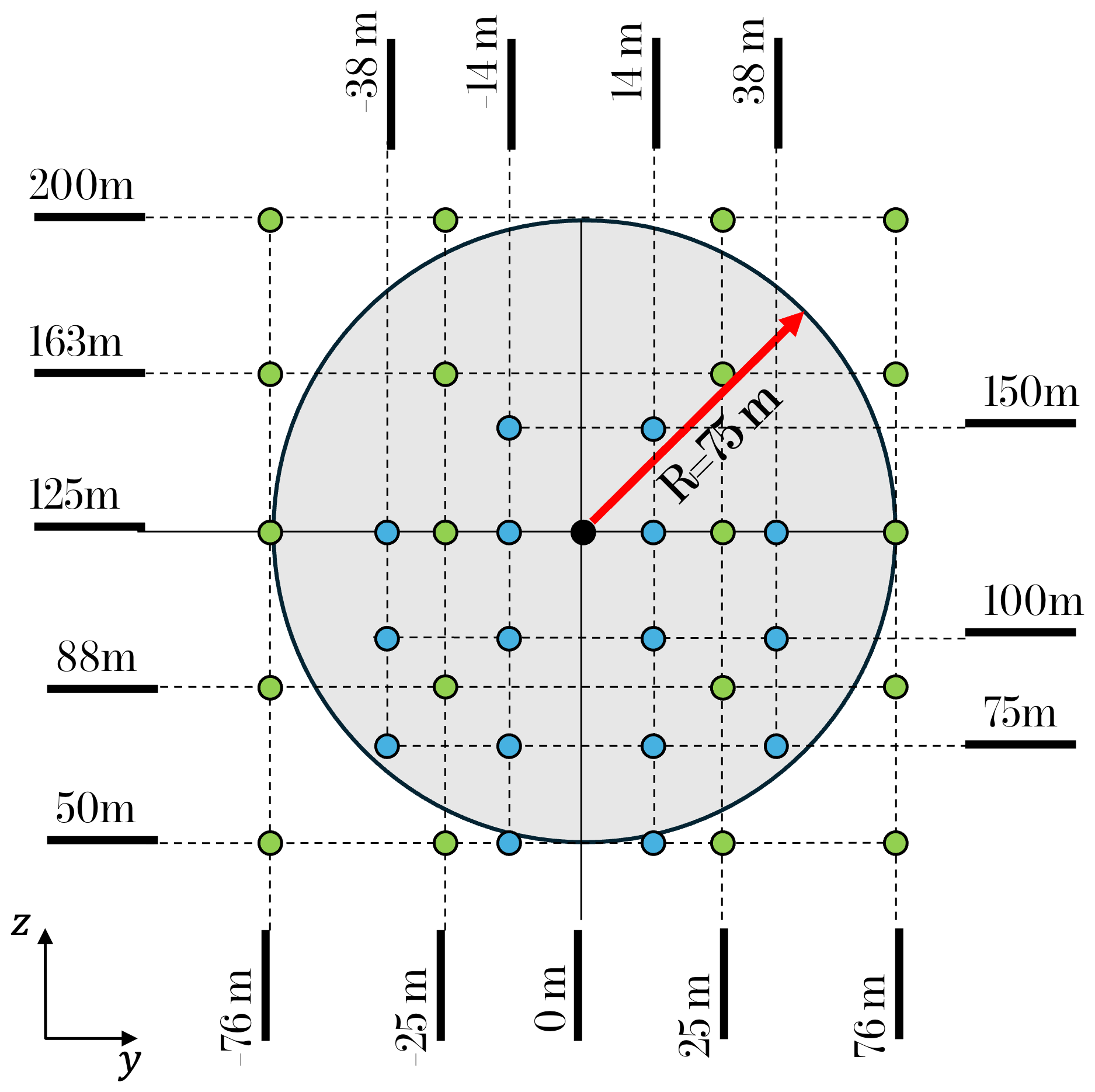
Figure 4 Schematic representation of the GROWIAN spatial grid. The blue circles show the original GROWIAN arrangement. The green circles show the locations of the stretched grid used for BEM simulations of a WT. The gray area depicts the WT model to be simulated with hub height at 125 m and rotor diameter of 149 m.

4 Results and discussion

This section presents the results of the two objectives of our investigation: the comparisons between the CoWP and the bending moments at the main shaft of the WT and the stochastic modeling of the CoWP. In Sect. 4.1, the results from the standard-modeled Kaimal data are shown. In Sect. 4.2, the investigation of the atmospheric GROWIAN measurements is presented. The analysis of the two data sets is performed as follows: the two components of the CoWP$=\mathit{\{}{\mathrm{CoWP}}_y,{\mathrm{CoWP}}_z\mathit{\}}$ are calculated from the wind fields according to Eq. (4), with the hub location, i.e., equivalent to the location of the main shaft, as the reference point (y₀, z₀). The Langevin stochastic approach described in Sect. 2.3 is then applied to model random signals of the CoWP. The characteristics of the original CoWP, the modeled CoWP, and the BEM-simulated bending moments $\mathbf{T}=\mathit{\{}{T}_{\mathrm{yaw}},T_{\mathrm{tilt}}\mathit{\}}$ at the main shaft of the WT are compared. For the comparison, the statistics over time, as well as the DEL, are analyzed.

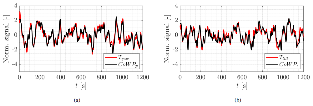
Figure 5 20 min excerpts of the CoWP and the bending moments at the main shaft of a WT. (a) T_yaw and CoWP_y and (b) T_tilt and CoWP_z. The signals are normalized and low-pass filtered.

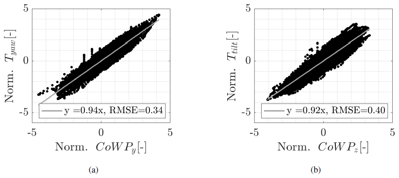
Figure 6 CoWP against the bending moments plotted as (CoWP(t), T(t)) for each time step t of the time series. (a) T_yaw and CoWP_y and (b) T_tilt and CoWP_z. The gray lines depict linear fittings $T=a\left(\mathrm{CoWP}\right)+b$. The values of the root mean square error (RMSE) are shown in the legends. The signals are normalized and low-pass filtered.

In Schubert et al. (2025) it has been shown that the CoWP can be used as a description of wind structures with temporal scales larger than 10 s. Accordingly, the correlation to the bending moments is limited to the low-frequency component. Therefore, to discard the high-frequency content, the signals are low-pass filtered. This applies to both the bending moments and the CoWP. The filter is a finite impulse response (FIR) filter with a cutoff or pass-band frequency f_cutoff. The value of f_cutoff should be lower than the rotational frequency P of the WT. In this way, the effect of gravitational loads from the rotating blades (i.e., P and 3P) is averaged out. Here, a 0.1 Hz cutoff frequency is applied. For comparability, the signals have also been normalized to have a mean of 0 and a standard deviation equal to 1. The comparisons presented in the following sections are made using the signals of the CoWP and the bending moments after frequency filtering and normalization.

4.1 The CoWP from standard Kaimal wind fields

4.1.1 The CoWP and the bending moments at the main shaft

We start by comparing the CoWP calculated from the Kaimal wind fields and the bending moments T from the BEM simulations. Figure 5 shows 20 min excerpts of the time series of the CoWP and the bending moments. In panel a, CoWP_y and T_yaw are shown, and in panel b, CoWP_z and T_tilt are shown. The observed correlation between the time series of the CoWP and the bending moments is quantified in Fig. 6. Each time step in the time series is represented by a point (CoWP(t), T(t)). In panel a, T_yaw and CoWP_y are shown, and in panel b, T_tilt and CoWP_z are shown. The observed linear behavior with a slope of approximately 0.93 quantifies the strong correlation between the normalized CoWP, which characterizes particular structures within the wind field, and the normalized bending moments experienced by the WT interacting with such a wind field. These correlations obtained from the standard Kaimal wind field corroborate the findings presented in Schubert et al. (2025), where the CoWP calculated from atmospherically measured data demonstrated correlation coefficients of up to 0.9 with the corresponding BEM-simulated yaw and tilt bending moments at the main shaft. A turbine-specific transfer function for rescaling the normalized values of the CoWP to magnitudes of the low-frequency component of operational bending moments would be necessary for the assessment of the loads in engineering applications. Such a transfer function will therefore depend on the structural properties of the WT and particular control mechanisms.

As a further statistical comparison, Fig. 7 shows the probability density functions (PDFs) of the CoWP and of the bending moments, taking into account all the simulated data. It should be noted that the rare large events, depicted by the tails of the PDFs, are in good agreement.

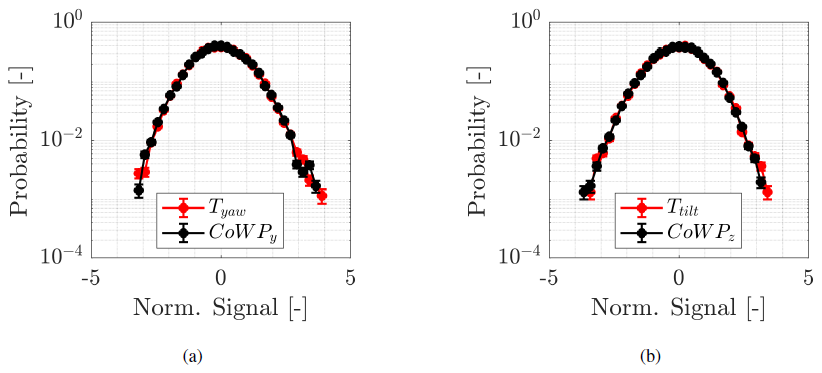
Figure 7 PDFs of the CoWP and the bending moments at the main shaft of a WT. (a) T_yaw and CoWP_y and (b) T_tilt and CoWP_z. The signals are normalized and low-pass filtered.

Now that we have proven the strong correlation between the dynamics of the low-frequency content of the CoWP and the bending moments, we continue by introducing the DEL_CoWP. The DEL_CoWP follows from Eq. (5) as

$$\begin{array}{}\text{(12)}& {\mathrm{DEL}}_{\mathrm{CoWP}}={\left({\displaystyle \frac{{\sum }_{i=\mathrm{1}}^n\left(n_{i,\mathrm{CoWP}}{s}_{i,\mathrm{CoWP}}^m\right)}{N_f}}\right)}_T^{m^{-\mathrm{1}}},\end{array}$$

where the number of cycles, n_i,CoWP, and the amplitudes, s_i,CoWP, are derived from the CoWP signals.

In Schubert et al. (2025), it was demonstrated that high values of the DEL are driven by significantly large-amplitude events in the low-pass-filtered time series of the loads. Additional proof of this correspondence is given in Appendix A. Accordingly, large-amplitude events in the signals of the CoWP will result in high values of DEL_CoWP.

Good agreement between the DEL and the DEL_CoWP implies that estimations of the low-frequency events of the bending moments at the main shaft of a WT can be accomplished purely from the estimation of the CoWP from the incoming wind field. Figure 8a and b show the correlation plots of the resulting time-resolved DEL and DEL_CoWP obtained through an averaging of time T=60 s and a coefficient m=10. Their statistics are summarized in the box plots in c and d. The DEL and DEL_CoWP are calculated in a and c from CoWP_y and T_yaw and in b from CoWP_z and T_tilt. A lower correlation is obtained for the DEL and DEL_CoWP in the vertical direction in panel b compared to the horizontal component shown in panel a. The lower correlation is explained by the more scattered results within the correlation of the time series of the T_tilt and the CoWP_z shown in Fig. 6. There, a value of RSME=0.40 indicates a higher degree of scattering for T_tilt compared to an RSME=0.34 for T_yaw. Overall, the data in Fig. 8 reveal very good agreement between the DEL and DEL_CoWP in a statistical sense. Although some spread of the data is observed, the statistics and correlation are consistent. In an aggregate sense, these results indicate an equivalence between the CoWP and the bending moments. The validity of the method has been proven for the rated power regime of the WT.

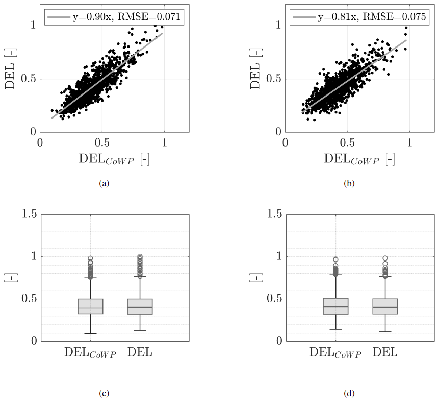
Figure 8 Comparison between the DEL and DEL_CoWP. Correlation plots and box plots for CoWP_y and T_yaw in (a) and (c) and CoWP_z and T_tilt in (b) and (d). The gray lines in (a) and (b) depict linear fittings. The values of the RMSE are shown in the legends. In the box plots in (c) and (d), the horizontal line inside each box shows the median, and the bottom and top edges indicate the 25th (P₂₅) and 75th (P₇₅) percentiles. The whiskers indicate the most extreme data points. They are calculated as $P_{\mathrm{25}}-(\mathrm{1.5}\times \mathrm{IQR})$ and $P_{\mathrm{75}}+(\mathrm{1.5}\times \mathrm{IQR})$, where IQR is the interquartile range $\mathrm{IQR}=P_{\mathrm{75}}-P_{\mathrm{25}}$. The markers show outliers. The DEL and DEL_CoWP are calculated with m=10 over periods T=60 s, with 30 s overlapping between two consecutive periods. The signals are normalized and low-pass filtered.

It is essential to acknowledge that the discussion of the DELs presented in our work is exclusively focused on the DELs from the low-frequency component of the signals. This choice is based on a particular interest of our research partners. In order to assess the complete DELs (e.g., from both the low- and the high-frequency load events), it is necessary to establish an additional model to incorporate the contribution from the high-frequency signal. In this direction, a simple surrogate stochastic model has shown satisfactory results. The characteristics of the original high-frequency load signal are well reproduced. The proposed stochastic model for the high-frequency signals, calculations of the differences between the DELs from the low- and high-frequency load components, and total DELs are shown in Appendix B.

4.1.2 Stochastic reconstruction of the CoWP

We now apply the stochastic Langevin approach introduced in Sect. 2.3 as a method for characterizing the low-frequency dynamics of the CoWP from the Kaimal wind fields. The two-dimensional stochastic differential equations (see Eq. 9) are thus applied for $\mathrm{CoWP}\left(t\right)=\mathit{\left\{}{\mathrm{CoWP}}_y\right(t),{\mathrm{CoWP}}_z(t\left)\mathit{\right\}}$. Since the two components CoWP_y(t) and CoWP_y(t) proved to be uncorrelated, i.e., $D_{\mathrm{12}}^{\left(\mathrm{2}\right)}=D_{\mathrm{21}}^{\left(\mathrm{2}\right)}=\mathrm{0}$, the coefficients D^(1,2) are independently estimated from the time series of CoWP_y and CoWP_z according to Eqs. (7) and (8). The results of the calculation of the correlation function 〈CoWP_i(t) CoWP_j(t+τ)〉 for $i=\mathrm{1},\mathrm{2}$ are shown in Appendix C.

The results of the coefficients D^(1,2) are shown in Fig. 9. The linear dependence of the drift coefficients D⁽¹⁾ in a is clear for the two components CoWP_y and CoWP_z. An almost-constant diffusion term D⁽²⁾ is observed in b for the two components.

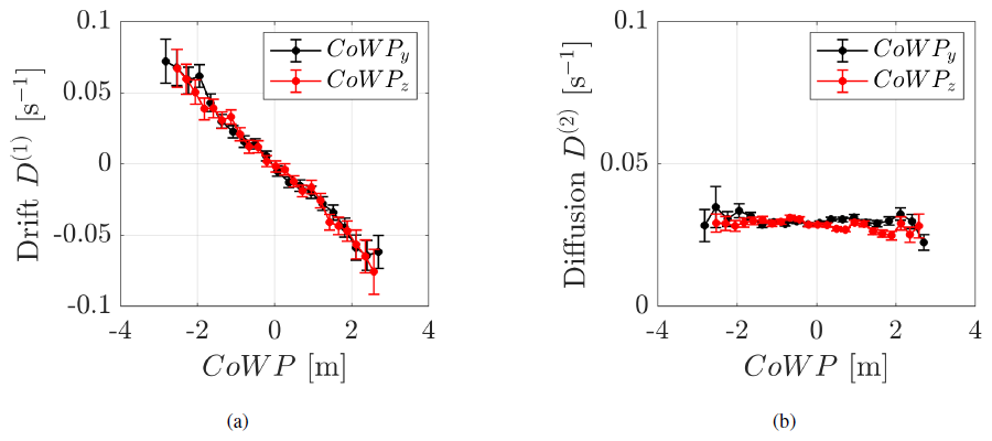
Figure 9 Langevin approach of the CoWP from Kaimal wind fields. (a) Drift coefficient D⁽¹⁾ and (b) diffusion coefficient D⁽²⁾. The vertical component CoWP_y is shown in black, and the horizontal component CoWP_z is shown in red.

The estimated D⁽¹⁾ and D⁽²⁾ are used for the reconstruction of synthetic time series (CoWP_R) via the stochastic integration of Eq. (9). A signal CoWP_R with a length of 4.7×10⁴ s is reconstructed.

For a first visual comparison between the original and the reconstructed signal, the filtered but non-normalized trajectories of the CoWP and CoWP_R in the y–z plane are shown in Fig. 10. Symmetric paths, i.e., comparable magnitudes in the two directions y and z, are observed for CoWP and CoWP_R.

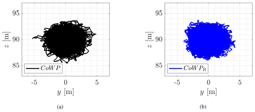
Figure 10 Trajectories on the y–z plane of (a) the original CoWP calculated from the Kaimal data and (b) the stochastically reconstructed signal CoWP_R. The data of both CoWP and CoWP_R for plotting the trajectories in (a) and (b) are intentionally not normalized.

Note that due to the stochastic reconstruction, temporal correlation is not expected between the two signals. However, a statistical similarity should be present. This is shown in Fig. 11, which compares the PDF of the signals. After filtering and normalization, the results of the BEM-simulated bending moments at the main shaft are also included: in a, the components in the horizontal y direction and, in b, the components in the vertical z direction.

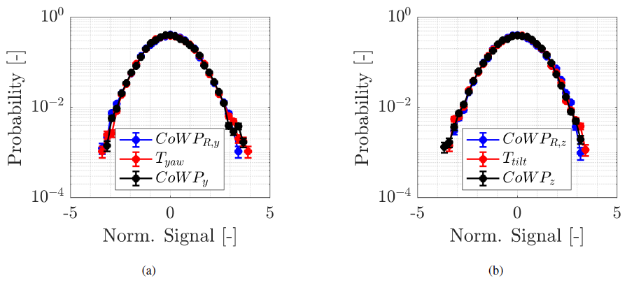
Figure 11 PDF of the CoWP, CoWP_R, and bending moments T. (a) CoWP_R,y, CoWP_y, and T_yaw. (b) CoWP_R,z, CoWP_z, and T_tilt. The signals are normalized and low-pass filtered.

To characterize the similarity of the signals in more detail, we also investigate the statistics of their increments or their variations for a given timescale τ. The increments are defined as $\mathrm{\Delta }{x}_{\mathit{\tau }}\left(t\right)=x(t+\mathit{\tau })-x\left(t\right)$ for a given signal x(t) and include two-time correlations like the autocorrelation or the power spectrum (Morales et al., 2012). Figure 12 shows the excellent agreement in the increment statistics of ΔCoWP_τ, ΔCoWP_R,τ, and ΔT_τ for values of $\mathit{\tau }=(\mathrm{5},\mathrm{10},\mathrm{20},\mathrm{30})\text{s}$. The components in the horizontal y direction and in the vertical z direction are shown in the upper and lower rows, respectively.

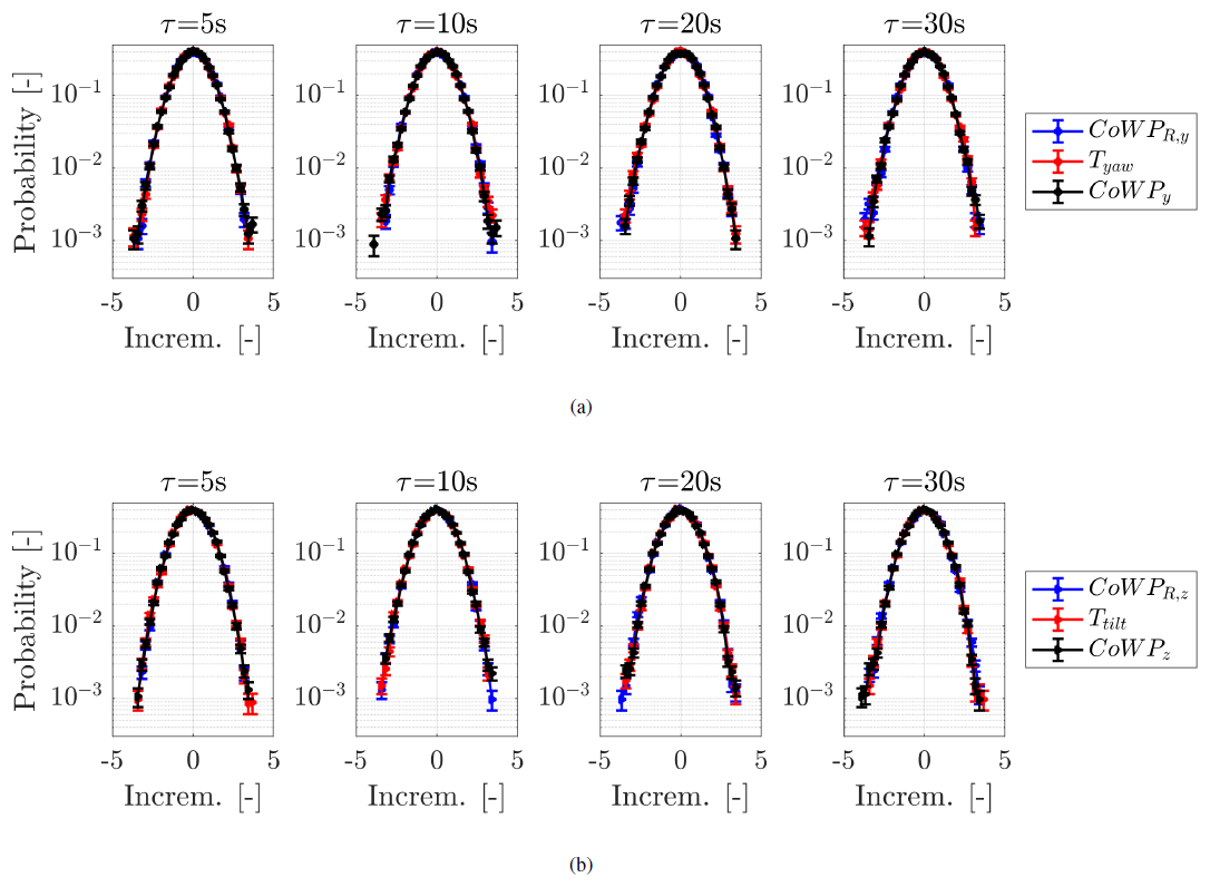
Figure 12 PDFs of the increments with $\mathit{\tau }=(\mathrm{5},\mathrm{10},\mathrm{20},\mathrm{30})\text{s}$. (a) Upper row, horizontal component: ΔCoWP_y,τ, $\mathrm{\Delta }{\mathrm{CoWP}}_{\mathrm{R},y,\mathit{\tau }}$, and ΔT_yaw,τ. (b) Lower row, vertical component: ΔCoWP_z,τ, $\mathrm{\Delta }{\mathrm{CoWP}}_{\mathrm{R},z,\mathit{\tau }}$, and ΔT_tilt,τ. The time series are normalized and low-pass filtered.

Finally, we show in Fig. 13 the agreement in the resulting DEL, DEL_CoWP, and DEL${}_{{\mathrm{CoWP}}_{\mathrm{R}}}$ through box plots. A subindex “R” refers to the reconstructed signal (a – the components in the horizontal y direction; b – the components in the vertical z direction). As observed from the box plots, the distributions of the DEL${}_{{\mathrm{CoWP}}_{\mathrm{R}}}$ from the stochastically reconstructed signal CoWP_R reproduce the distributions of both the DEL_CoWP from the original CoWP and the DEL from the BEM-simulated signals quite accurately.

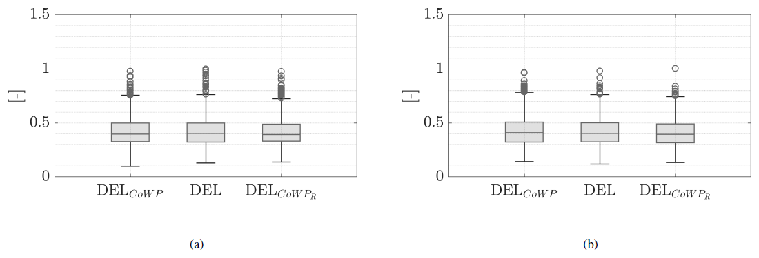
Figure 13 Box plots of the DEL_CoWP, DEL, and DEL${}_{{\mathrm{CoWP}}_{\mathrm{R}}}$ from normalized and filtered signals of (a) CoWP_y, T_yaw, and CoWP_R,y and (b) CoWP_z, T_tilt, and CoWP_R,z. The DELs are calculated over periods T=60 s, with 30 s of overlap and with a coefficient m=10. The lines defining each box show the median, and the bottom and top edges indicate the 25th (P₂₅) and 75th (P₇₅) percentiles. The whiskers indicate the most extreme data points. They are calculated as $P_{\mathrm{25}}-(\mathrm{1.5}\times \mathrm{IQR})$ and $P_{\mathrm{75}}+(\mathrm{1.5}\times \mathrm{IQR})$. The markers show outliers.

4.2 The CoWP from atmospheric GROWIAN measurements

Next, we use the atmospheric GROWIAN wind fields described in Sect. 3 to calculate the CoWP, to simulate the BEM bending moments at the main shaft, and to apply the stochastic Langevin model for the reconstruction of random data. The results are presented in the same sequence as done for the Kaimal data in the previous section.

4.2.1 The CoWP and the bending moments at the main shaft

Figure 14 shows the correlation plots between the CoWP and the bending moments T: in a, T_yaw and CoWP_y and, in b, T_tilt and CoWP_z. The coefficients of the linear fittings agree with the correlation coefficients of around 0.9 reported in Schubert et al. (2025), where all the available GROWIAN wind fields are investigated. Differently, in this paper, we only investigate a subset of the atmospheric data, conditioned by the mean wind speed, turbulence intensity, and shear exponent, as described in Sect. 3. The correlation between the CoWP and the bending moments is slightly decreased compared to the standard-modeled wind data shown in Fig. 6. In particular, loops are observed in Fig. 14 for the two components, a and b. Such loops correspond to intervals where more severe wind conditions affect the WT than those we find in the Kaimal wind data. Over those intervals, significant differences in the wind speed are observed in the spatial domain (i.e., over the rotor plane). As a result, divergences in calculating the CoWP and the bending moments are obtained. Examples of such severe wind conditions within the atmospherically rescaled GROWIAN fields are shown in Appendix D.

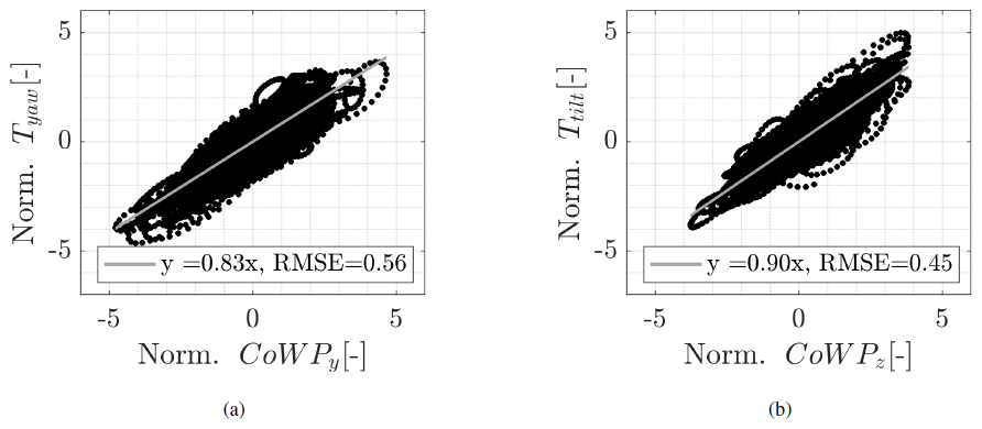
Figure 14 CoWP against the bending moments T at the main shaft of a WT plotted as (CoWP(t), T(t)) for each time step t of the time series. (a) T_yaw and CoWP_y and (b) T_tilt and CoWP_z. The gray lines depict linear fittings. The values of the RMSE are shown in the legends. The time series are normalized and low-pass filtered.

4.2.2 Reconstructing the CoWP from atmospheric wind data

The results of the coefficients D^(1,2) from the stochastic Langevin method, applied to the CoWP from the GROWIAN measurements, are shown in Fig. 15. Interestingly, the diffusion coefficients D⁽²⁾ in b are clearly not constant. This behavior is called multiplicative noise and is significantly stronger for the vertical component CoWP_z. In contrast, pure additive noise was obtained for the modeled Kaimal fields in Fig. 9. Moreover, the diffusion coefficient D⁽²⁾ of the CoWP_z from Kaimal data with shear showed pure additive noise (see Appendix E). This effect in D⁽²⁾ is a consequence of the different wind fields and shows that the Kaimal data lead to simpler noise. In contrast, atmospheric wind data have more complicated deterministic and noise contributions.

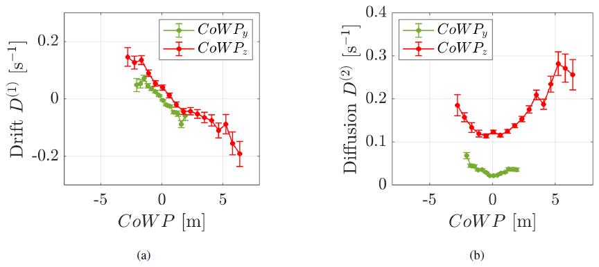
Figure 15 Langevin approach of the CoWP from GROWIAN wind fields. (a) Drift coefficient D⁽¹⁾ and (b) diffusion coefficient D⁽²⁾. The vertical component CoWP_y is shown in green, and the horizontal component CoWP_z is shown in red.

Figure 16 shows the trajectories of the CoWP and the CoWP_R in the y–z plane. For this representation, the time series are not normalized. Due to the shear, the movement of the CoWP in the vertical direction z is larger than in the horizontal direction y. This differs from Fig. 10, where symmetric trajectories in the two y–z directions are obtained for non-shear Kaimal wind fields.

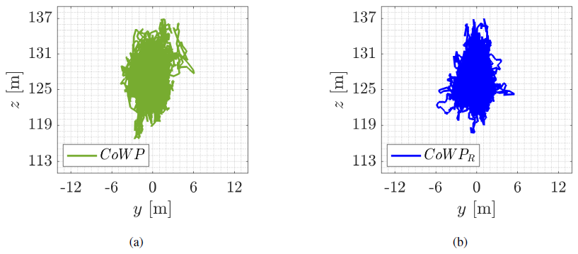
Figure 16 Trajectories on the y–z plane of (a) the CoWP from the original GROWIAN measurements and (b) the stochastically reconstructed signal CoWP_R. The data are not normalized.

Figure 17 shows the PDF of the signals. The time series of the BEM-simulated bending moments T_yaw and T_tilt are also included: in a, for the horizontal y component and, in b, for the vertical z component. We see that the stochastic model reproduces the statistics of the CoWP and bending moment very well. The PDFs of Fig. 17 show additional structures like skewness and small bumps. These structures are the consequence of the nonlinearities of D^(1,2) in Fig. 9 (see also the stationary solution of the Fokker–Planck equation, which corresponds to the Langevin equation, Risken, 1996).

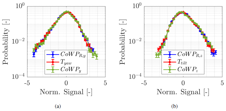
Figure 17 PDF of the CoWP, CoWP_R, and bending moments T. (a) CoWP_y, T_yaw, and CoWP_R,y. (b) CoWP_z, T_tilt, and CoWP_R,z. The signals are normalized and low-pass filtered.

As a higher-order statistical feature, Fig. 18 shows the PDFs of the increments ΔCoWP_τ, ΔCoWP_R,τ, and ΔT_τ for values of $\mathit{\tau }=(\mathrm{5},\mathrm{10},\mathrm{20},\mathrm{30})\mathrm{s}$ (a – the components in the horizontal y direction; b – the components in the vertical z direction).

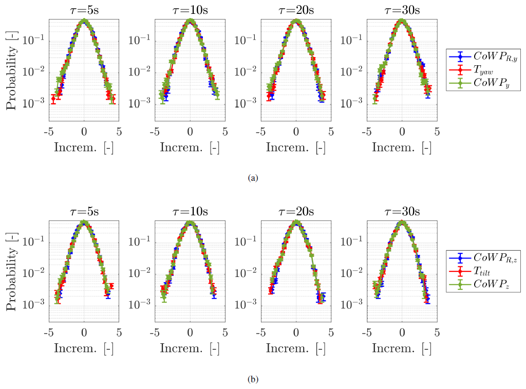
Figure 18 PDFs of the increments with $\mathit{\tau }=(\mathrm{5},\mathrm{10},\mathrm{20},\mathrm{30})\mathrm{s}$. (a) Horizontal component: ΔCoWP_y,τ, $\mathrm{\Delta }{\mathrm{CoWP}}_{\mathrm{R},y,\mathit{\tau }}$, and ΔT_yaw,τ. (b) Vertical component: ΔCoWP_z,τ, $\mathrm{\Delta }{\mathrm{CoWP}}_{\mathrm{R},z,\mathit{\tau }}$, and ΔT_tilt,τ. The time series are normalized and low-pass filtered.

Finally, Fig. 19a and b show the correlation plots of the DEL and DEL_CoWP. In c and d, the box plots describing their statistics are shown. The box plots of the DEL${}_{{\mathrm{CoWP}}_{\mathrm{R}}}$ in the two components are also included. The DEL and DEL_CoWP are calculated in a and c from CoWP_y and T_yaw and in b from CoWP_z and T_tilt. All time series are normalized and filtered.

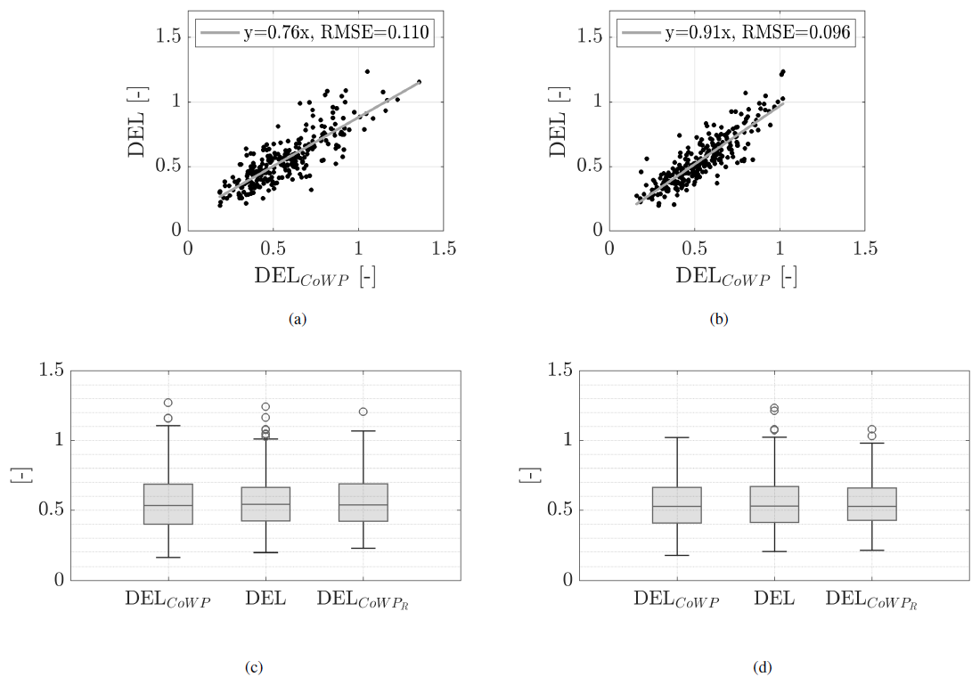
Figure 19 Comparison between the DEL_CoWP, DEL, and DEL${}_{{\mathrm{CoWP}}_{\mathrm{R}}}$. Correlation plots and box plots for CoWP_y and T_yaw are shown in (a) and (c), and those for CoWP_z and T_tilt are shown in (b) and (d). The gray lines in (a) and (b) depict linear fittings. The values of the RMSE are shown in the legends. In the box plots in (c) and (d), the horizontal line inside each box shows the median, and the bottom and top edges indicate the 25th (P₂₅) and 75th (P₇₅) percentiles. The whiskers indicate the most extreme data points. They are calculated as $P_{\mathrm{25}}-(\mathrm{1.5}\times \mathrm{IQR})$ and $P_{\mathrm{75}}+(\mathrm{1.5}\times \mathrm{IQR})$. The markers show outliers. The DELs are calculated with m=10 over periods T=60 s, with 30 s overlapping between two consecutive periods. The signals are normalized and low-pass filtered.

The correlations between the low-pass-filtered and normalized signals of the CoWP and the bending moments shown in Fig. 14 and between the DEL_CoWP and DEL shown in Fig. 19 for the atmospheric GROWIAN data are slightly lower compared to the modeled Kaimal data in Figs. 6 and 8. The higher complexity of real wind fields includes wind events characterized by stronger differences in wind speed over the y–z plane within the stretched wind fields, which likely explain such particular discrepancies. However, Figs. 17, 18, and 19 show good agreement between the statistical properties and the DEL estimations between the original and the reconstructed signals of the CoWP and the simulated bending moments from the atmospherically measured GROWIAN data. These findings are in agreement with the results shown in Sect. 4.1 for the standard-modeled Kaimal data. Therefore, it was demonstrated that the description of the dynamics provided by the coefficients D^(1,2) from the CoWP can be used as parameters for modeling the low-frequency signals of the tilt and yaw bending moments at the main shaft of a WT.

5 Conclusions and outlook

A comparison between the low-frequency content of the center of wind pressure (CoWP) as a feature of a turbulent wind field and the low-frequency content of the BEM-simulated bending moments at the main shaft of a wind turbine, e.g., yaw and tilt, is performed. A strong correlation between these large-scale structures of the CoWP and bending moments has been quantified in terms of statistical properties, correlation factors, and damage equivalent load (DEL). This correlation is consistent with the results reported in the studies by Schubert et al. (2025) and Moreno et al. (2024), and it has been shown to be valid for wind fields from both atmospheric measurements and standard models. As a consequence of this correlation, a comprehensive description of the CoWP from a particular wind field (e.g., site-specific) might serve as a surrogate estimator of the low-frequency load events of the tilt and yaw bending moments at the main shaft of an operating wind turbine.

A step further is the utilization of a comprehensive understanding of the dynamics of the CoWP from wind data, with the objective of modeling loads. The stochastic Langevin approach has been proposed as a method for characterizing the dynamics of the CoWP. More interestingly, the method has been reverse-applied for the stochastic reconstruction of synthetic signals. The resulting statistics from the reconstructed signals and their estimated DELs have been shown to be comparable to those of the original CoWP and, more significantly, to those from the BEM-simulated bending moments. Consequently, the stochastic Langevin approach applied to the CoWP has been proven as a surrogate method for estimating the low-frequency content of the moments at the main shaft. In particular, the Langevin approach significantly reduces computational cost by solving only a one- or two-dimensional stochastic equation instead of calculating a wind field at many different spatial points and its interaction with the turbine model. This has the potential to reconstruct very long modeled load data. This feature is essential for the assessment of tilt and yaw bending moments when particularly large amounts of simulated data are required, e.g., for 25-year lifetime predictions under multiple wind conditions, and the computational costs associated with costly BEM simulations would thus be significantly reduced.

However, the development of lifetime predictions in engineering applications necessitates the incorporation of additional elements in conjunction with the proposed stochastic method for modeling the low-frequency component of the loads. Initially, a turbine-specific transfer function for rescaling the CoWP to the magnitudes of the low-frequency component of the bending moments should be derived. Secondly, a numerical model of the high-frequency component of the loads is required. A stochastic Gaussian model has been demonstrated to be a viable approach. Thirdly, site-specific wind characteristics should be considered. These characteristics should include long-term standard wind conditions, such as the annual Weibull distribution of the wind speed. Additionally, spatial descriptions (i.e., perpendicular to the main flow) of the wind structures are necessary to describe the dynamics of the CoWP at the given location. These spatial descriptions may be derived either from measured data over a two-dimensional area (e.g., using lidar techniques) or from accurately modeled wind data, which includes realistic information about the wind structures in the spatial domain. Once the three complementary elements have been resolved, the complete prediction of the yaw and tilt bending moments at the main shaft of a turbine can be applied as follows: site-specific wind data over relatively short intervals (e.g., 10 min), which are used for the calculation of the CoWP. Subsequently, the dynamics of the large-scale wind structures described by the CoWP are derived by using the Langevin stochastic approach. The parameters of the Langevin model for the specific wind conditions (i.e., drift and diffusion coefficients) are then estimated. Next, stochastic realizations of the low-frequency component of the loads are generated by combining the dynamics of the CoWP and the previously determined turbine-specific transfer function. Afterwards, the high-frequency component is modeled. Subsequently, the high- and low-frequency load signals, which have been modeled independently, are combined. Finally, the long-term distribution of the mean wind speed $p\left(\stackrel{\mathrm{‾}}{u}\right)$ at the specific location is used to assess the entire lifetime damage of the bending moments (i.e., by applying the standard IEC procedure for load assessment based on mean wind speed binning and design load cases).

In the context of improved descriptions of atmospheric turbulent wind, including the statistical and dynamical properties of the CoWP from atmospherically measured data into standard wind models could prove to be of significant value. Since the wind industry currently uses standard wind models for design and certification processes, the incorporation of atmospheric information would enhance the understanding of aerodynamic interactions and enable more accurate load assessment of the turbines. For instance, wind structures such as gusts are assumed by standard wind models to be homogeneous in space. The CoWP has the capacity to grasp localized wind structures over the rotor plane. A parameterization of the dynamics of the CoWP from atmospheric wind would thus describe the realistic and likely non-homogeneous spatial characteristics of the gusts. A comparison of the drift and diffusion coefficients derived from standard wind model data and measured data reveals that different characteristics of the wind fields are mapped into the Langevin equations. Consequently, the availability of local wind data enables the estimation of site-specific wind characteristics and the subsequent development of the stochastic load model.

This paper shows that the CoWP and its stochastic modeling represent a promising new tool for estimating the large-scale dynamics of specific loads at the wind turbine. The validity of this load estimation has been demonstrated in the context of DELs. The dynamic response of modern wind turbines with increased size gives additional relevance to wind structures over the rotor plane. The larger areas covered by these larger rotors are likely to include inhomogeneities (e.g., severe differences in wind speed) over the rotor. In this direction, the CoWP and the stochastic approach delineated in our paper have the potential to serve as a tool for describing and modeling IEC extreme scenarios (i.e., with 50-year or 1-year return periods). Up to now, calibrating the magnitude of the CoWP to the loads requires BEM simulations, at least on a finite time window. The validity of the CoWP approach for other loads at different turbine components remains to be investigated. For a single blade, a rotational frame of reference could be helpful for the calculation of the CoWP. Based on the results presented in this paper, it is recommended that a comparable procedure be considered for any other load in the turbine. The initial step involves normalizing the signals and validating the correlation. Following this, a stochastic model is to be configured to analyze and reconstruct the dynamic load response.

Appendix A: Correlation between DEL and DEL_CoWP

The DEL_CoWP introduced in Eq. (12) is based on the conclusion stated by Schubert et al. (2025) that large-amplitude load events, lasting longer than 10 s, e.g., bump structures, drive large values of the DEL when using the Wöhler exponent m=10. We now present a different proof of this finding.

The aim is to compare the DEL between time series with and without particularly large-amplitude load events. Figure A1a shows an excerpt of 15 ×10³ s containing the results of the DEL from the time series of the yaw moment T_yaw. The horizontal red bars depict the period T=10 min over which the DEL is calculated. The largest DELs are identified and visually separated above the horizontal gray line. The respective time series T_yaw, from which the DELs are calculated, are shown in b. The darker highlighted load events at 3300, 3700, 3850, and 9800 s correspond to the largest DEL (over the gray line) in a. The zoomed-in plot in the lower part of b illustrates the load event at t≈9800 s.

Figure A2a shows a modified time series “T_yaw-Mod”, from which the large load events highlighted in Fig. A1b have been removed. The resulting DELs from T_yaw-Mod are shown in b. The comparison between the DELs in Figs. A1a and A2b, i.e., from the two versions of the time series T_yaw, confirms that large-amplitude events in the signal induce large values of the DEL. Therefore, an accurate fatigue assessment of the moments T based on the DEL, as the standard procedure within the wind industry, requires an accurate description of such large-amplitude loading events. The DEL_CoWP is proposed in Sect. 4.1 as an approach for predicting these events on the loads from the wind field.

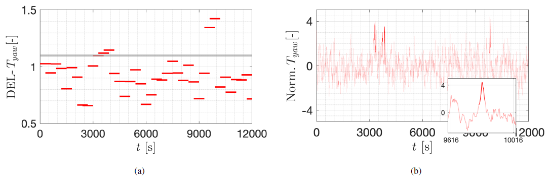
Figure A1 Damage equivalent loads (DELs) of the yaw moment signal T_yaw from BEM simulations. (a) DELs of T_yaw. The horizontal gray line at DEL =1.1 visually separates the few largest DELs. The DELs are calculated with m=10 over periods T=10 min. An overlapping period of 5 min is considered between two consecutive intervals. The length of the horizontal red bars depicts the periods T. (b) Time series T_yaw with large events highlighted, which induce the largest DEL in (a). The length of such identified load events within the time series T_yaw is considered to be 20 s, over which the peak amplitude is included. The event at t≈9800 s is detailed in the zoomed-in plot. The time series T_yaw are calculated by BEM simulations of the 5 MW NREL turbine (see Sect. 3). The time series T_yaw are low-pass filtered with cutoff f=0.1 and normalized to a mean of 0 and standard deviation equal to 1.

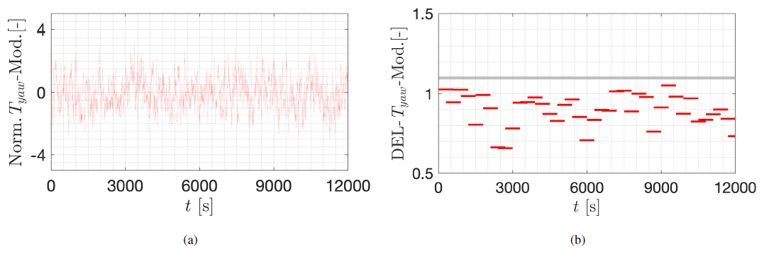
Figure A2 Damage equivalent loads (DELs) of a modified signal of the yaw moment “T_yaw-Mod” from BEM simulations. (a) Time series “T_yaw-Mod” from which the highlighted intervals in Fig. A1b have been removed. (b) DELs of T_yaw-Mod. The horizontal blue line at DEL =1.1 is kept as a reference. The DELs are calculated with m=10 over T=10 min. An overlapping period of 5 min is considered between two consecutive intervals. The length of the horizontal red bars depicts the length of T.

Appendix B: DELs from low- and high-frequency components of the loads

The contribution of the low- and high-frequency components of the load signal to the DELs of the total load is investigated. Therefore, different components of the load signal are independently investigated. The low-frequency component (“low freq.”) corresponds to the low-pass-filtered load described in Sect. 4, with a cutoff frequency of f_cutoff=0.1 Hz. The high-frequency component (“high freq.”) corresponds to the load fluctuations with a frequency over f_cutoff. The total load (“total”) is the estimated load from BEM simulations, which aggregates both the high- and the low-frequency components.

Figure B1a shows the DELs of the components of the load over an excerpt of 1200 s. Each of the horizontal bars represents the period T=60 s over which the DEL is calculated. A fourth signal, “sum L+H”, is included in the comparison. It corresponds to the combination of the DELs (i.e., not the time series) from the low- and high-frequency signals as

$$\begin{array}{}\text{(B1)}& \left({\mathrm{DEL}}_{\mathrm{SumL}+\mathrm{H}}\right)=\mathit{\alpha }\left({\mathrm{DEL}}_{\mathrm{Low}}\right)+\mathit{\beta }\left({\mathrm{DEL}}_{\mathrm{High}}\right),\end{array}$$

calculated for each period T. The parameters α and β are fitting parameters to achieve ${\mathrm{DEL}}_{\mathrm{SumL}+\mathrm{H}}\approx {\mathrm{DEL}}_{\mathrm{Total}}$. These parameters depend on the Wöhler coefficient m and the length T for the calculation of DEL_Low and DEL_High. In Fig. B1a, the parameters are α=1.2 and β=0.5. The values of the coefficients α and β from the load signals can be taken as weighting factors, indicating a dominating contribution of DEL_Low with respect to DEL_High. For the case shown, the proportion is approximately 2:1.

Figure B1b shows the correlation between the DELs of the total and the sum L+H signals. The correlation is calculated for the DELs along the entire data set (4.7×10⁴ s). Based on the strong correlation between the DELs in b, the DELs of the total load might be interpreted as a weighted sum of the individual DELs from the low- and high-frequency components.

The results in Fig. B1 show that, despite the dominance of the low-frequency contribution, both the low- and the high-frequency components have important contributions to the DELs of the total load signal. Therefore, for a complete calculation of the DELs on the WT, a second model for the high-frequency contribution is required. The use of Gaussian distributed noise is proposed as a first approach. Three random Gaussian realizations, “R1”, “R2”, and “R3”, with the statistics from the original high-frequency load signal, are generated. The considered statistics include not only the mean and standard deviation, but also the correlation and dominant frequency. Next, the three Gaussian realizations of the high-frequency fluctuations are added to the low-frequency component of the load. Then, the DELs are calculated.

Figure B2a shows a 20 min excerpt of the DELs. For comparison, the original total load, which is the sum of the original high-frequency and low-frequency components, is also compared. Figure B2b shows a box plot of the DELs over the entire time series (4.7×10⁴ s).

The comparability between the box plots in Fig. B2 shows that Gaussian noise, with a parameterized dominant frequency and correlation, can be used as a model for the high-frequency component of the load signals. Then, this Gaussian model for high-frequency fluctuations might be used in combination with our proposed model, based on the CoWP, which reproduced the low-frequency component of the load signal. Subsequently, an entire description of the load signals could be achieved. The joint use of these two models must be further validated by comparing them to the total simulated loads. For that, a transfer function is required to scale the magnitudes of the loads. The validation is out of the scope of this paper.

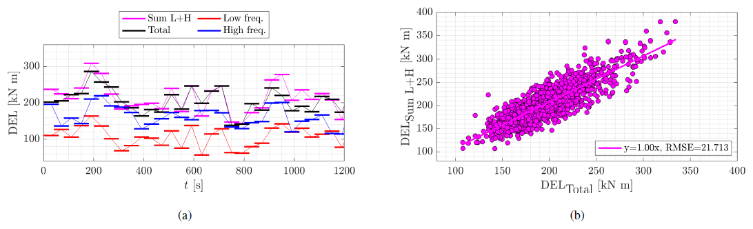
Figure B1 (a) 20 min excerpt of the DELs for the T_titlt signals at the main shaft. The length of the individual horizontal bars depicts the periods T. (b) Correlation plot between the total load and the sum of the DELs from the low- and high-frequency signals. The DELs are calculated with m=10 over periods of T=60 s with an overlap of 30 s between periods. The load signals are those calculated from BEM simulations of the 5 MW NREL WT with Kaimal fields, with $\stackrel{\mathrm{‾}}{u}=\mathrm{7}{\mathrm{m}\mathrm{s}}^{-\mathrm{1}}$ (see Sect. 3).

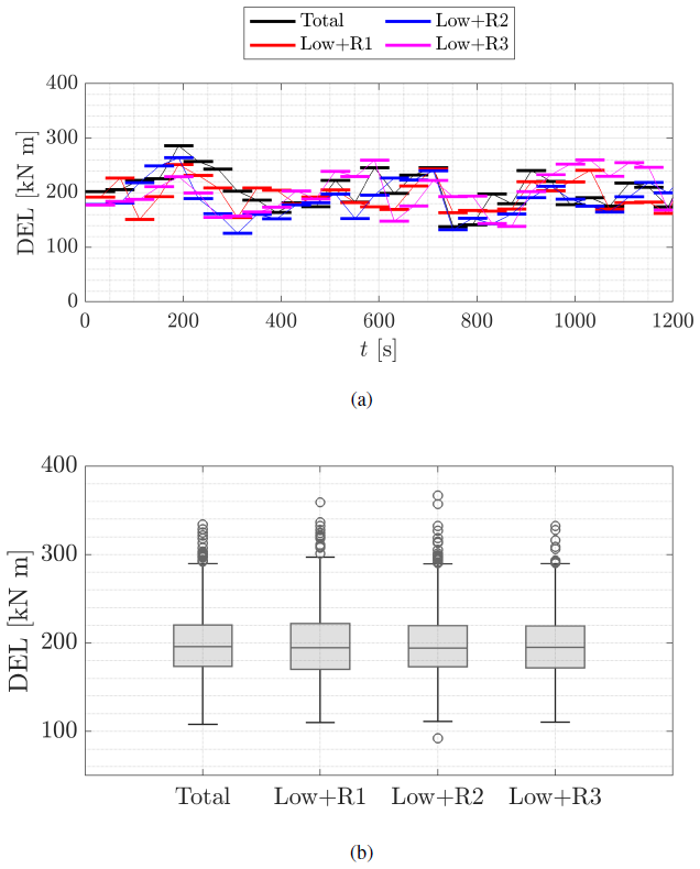
Figure B2 DELs of the total signals (low-frequency and high-frequency signals). (a) 20 min excerpt with individual DELs. (b) Box plots of the DELs along the entire time series. The four high-frequency signals (“high freq.”, “R1”, “R2”, and “R3”) have been added to the same low-frequency signal. The DELs are calculated with m=10 over periods of T=60 s with an overlap of 30 s between periods.

Appendix C: Correlation and structure function of the CoWP

Figure C1 shows the correlation function for the two components of the CoWP 〈CoWP_i(t) CoWP_j(t+τ)〉 for $i=y,z$. From the top to the bottom, the three rows show the correlation for i≠j, $i=j=y$, and $i=j=z$. The panels on the left (a, c, d) correspond to the modeled Kaimal data. The panels on the right (b, d, e) show the atmospherically measured GROWIAN data. The correlation is calculated for time lags $\mathit{\tau }=[-\mathrm{200},\mathrm{200}]$.

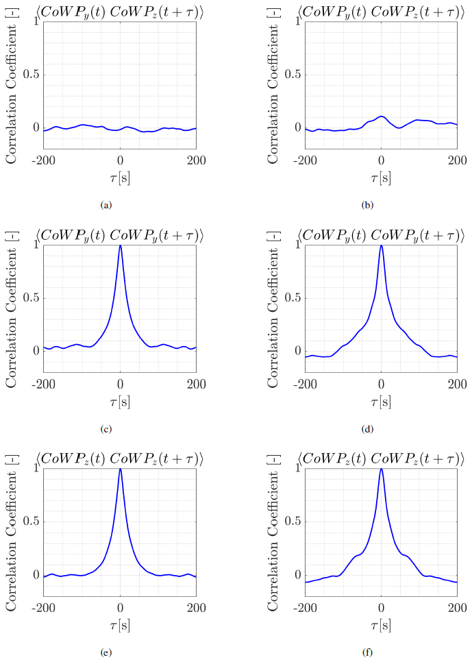
Figure C1 Correlation function for the two components of the CoWP 〈CoWP_i(t) CoWP_j(t+τ)〉 for $i=y,z$ and $\mathit{\tau }=[-\mathrm{200},\mathrm{200}]$. The modeled Kaimal data are shown in (a), (c), and (e), and the atmospheric GROWIAN data are shown in (b), (d), and (f).

Appendix D: “Special events” of the CoWP from GROWIAN data

In Fig. 14, particular loops are observed when correlating the CoWP and the tilt and yaw bending moments from atmospheric GROWIAN wind fields. Figure D1 shows three exemplary temporal sequences corresponding to some of the observed loops in the correlation plots. Short intervals of 4 s are shown. Panels a and b show sequences observed in the correlation between CoWP_y and T_yaw in Fig. 14a. Panel c shows a sequence observed in the correlation between CoWP_z and T_tilt in Fig. 14b. As observed in the three sequences, there are very strong differences in the wind speed over the rotor plane. The green dot shows the CoWP. The red dot shows a scaled version of the CoWP, which allows for better visualization. The scaling is done by subtracting a mean wind speed from all the points of the wind field. This subtraction is analogous to removing the mass of the beam when calculating the center of mass induced by external masses. In that way, larger distances of the CoWP with respect to the reference point are obtained.

The relatively large deviations of the CoWP depicted by the loops in Fig. 14 from the GROWIAN data suggest that the CoWP might be very sensitive to such extreme differences in the wind field over the y–z plane at a given time step.

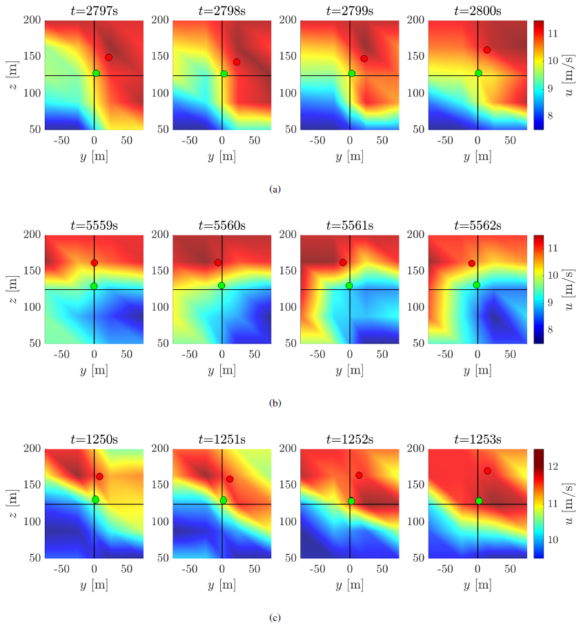
Figure D1 Temporal evolution of the GROWIAN wind field and the CoWP on the y–z plane. The wind speed $u(y,z,t)$ is color-coded. The green dot depicts the location of CoWP. For better visualization, the red dot depicts the location of a scaled version of the CoWP. The lines show the center lines of the grid, i.e., the reference location for calculating CoWP.

Appendix E: Characteristics of the CoWP from standard Kaimal wind fields with shear

The results of the drift and diffusion coefficients D^(1,2) from the stochastic Langevin method, applied to the CoWP from the GROWIAN measurements, are shown in Fig. 15. To investigate and compare the effect of the shear in the dynamics of the CoWP from standard-modeled wind fields, we calculated the coefficients D^(1,2) from Kaimal wind fields with a shear exponent of 0.2. The results are shown in Fig. E1. Interestingly, the superimposition of shear to the Kaimal wind fields results in additive noise only shifted towards higher heights.

Additionally, the trajectories of the CoWP on the y–z plane are shown in Fig. E2 for the original CoWP and a reconstructed signal CoWP_R from the Kaimal wind fields with shear. In comparison to the trajectories from the atmospheric GROWIAN data in Fig. 16, the trajectories of the CoWP from the shear Kaimal wind fields are symmetric in the y–z directions. Again, only a vertical shift is observed within the CoWP, including shear effects, compared to Fig. 10.

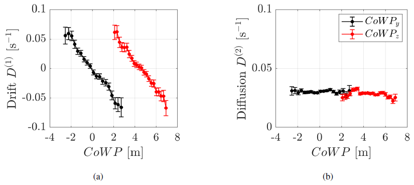
Figure E1 Langevin approach of the CoWP from Kaimal wind fields with a shear exponent of 0.2. (a) Drift coefficient D⁽¹⁾ and (b) diffusion coefficient D⁽²⁾. The vertical component CoWP_y is shown in black, and the horizontal component CoWP_z is shown in red.

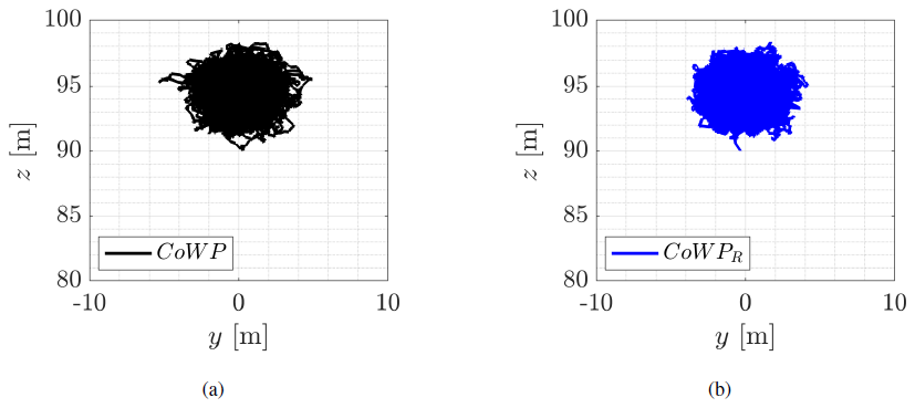
Figure E2 Trajectories on the y–z plane of (a) the CoWP from the original shear Kaimal wind fields and (b) the corresponding stochastically reconstructed signal CoWP_R. The data are not normalized.