Evaluating the impact of motion compensation on turbulence intensity measurements from continuous-wave and pulsed floating lidars

Floating lidar systems (FLSs) play a crucial role in offshore wind resource assessment, offering a cost-effective and flexible alternative to traditional meteorological masts. While wind speed and wind direction measurements from FLSs demonstrate high accuracy without further in-depth correction required, platform motion introduces systematic overestimation of turbulence intensity (TI), requiring compensation to ensure reliability.

This study presents the first published report of an offshore deployment of a pulsed FLS operating at 5 Hz effective sampling frequency with full deterministic motion compensation. A side-by-side comparison was conducted with a continuous-wave (cw) FLS of the same platform type under identical offshore conditions. Both systems were benchmarked against a met mast cup anemometer reference, with a fixed cw lidar included for plausibility checks.

Performance was evaluated using a comprehensive multi-metric framework, including regression analyses, absolute and relative error measures (MBE, MRBE, RMSE, RRMSE), representative TI error (Q90 error), and quantile-based distribution analysis. While it is well established that deterministic motion compensation improves TI estimates from floating cw lidars, this study demonstrates for the first time that the same approach, when applied to pulsed systems operating at 5 Hz, yields TI bias convergence with floating cw lidars relative to a met mast reference under identical offshore conditions. After compensation, floating cw and pulsed TI bias converged towards the cup reference with no systematic ranking, while the pulsed system showed a modest but consistent advantage in scatter-based metrics.

A central finding is that effective sampling frequency is a decisive configuration parameter for pulsed systems: empirical evidence demonstrates that a 5 Hz operation adequately resolves turbulence and motion timescales, achieving industry-relevant TI accuracy. In contrast, 1 Hz undersamples these processes and consistently overestimates TI, whereas 50 Hz cw scanning provides no decisive benefit beyond 5 Hz.

These results establish deterministic motion compensation as a transparent and effective baseline for offshore FLS turbulence assessment. For pulsed deployments, a 5 Hz configuration is sufficient, while residual scatter remains the main limitation. Future work should refine the compensation algorithm by accounting for lidar sensitivities and improving sensor synchronization, while broadening validation across platform types, sea states, and lidar configurations. Another important direction is the systematic comparison of different motion-compensation types under identical sea-state and platform-response conditions. Sensitivity studies of motion characteristics, atmospheric stability, and lidar parameters are also needed. Machine learning post-processing may be explored as a complementary tool to further reduce dispersion.

1 Introduction

Offshore wind energy has gained significant momentum as a key component of the global transition to renewable energy (WindEurope, 2024). Accurate site assessment is crucial for the successful development of offshore wind farms, as it directly impacts the feasibility, efficiency, and economic viability of these projects. Advanced wind measurement technologies, including meteorological mast (met mast) and remote sensing devices, play a pivotal role in understanding wind conditions over open water (Sempreviva et al., 2008).

Floating lidar systems (FLSs) represent an innovative advancement over met masts in offshore wind resource assessment (Gottschall et al., 2017). These buoy systems are designed to provide accurate and reliable measurements of wind speed, direction, and other meteorological and oceanographic parameters in harsh offshore environments where traditional met masts may be difficult to install and maintain. FLSs typically consist of one or more vertical profiling wind lidars mounted on or integrated into a floating platform. These systems are designed to operate autonomously, featuring self-sufficient power supplies, multiple communication systems, motion recording devices (inertial measurement units – IMUs), and various supplementary measurement instruments.

The Carbon Trust OWA Roadmap for the Commercial Acceptance of Floating LiDAR Technology (The Carbon Trust, 2018, also referred to as the OWA Roadmap) defines a structured approach to prove the accuracy, quality, and reliability of the individual FLS system in three stages of maturity. Herein defined key performance indicators (KPIs) focus on wind speed and wind direction data. While the IEC 61400-50-4 technical specification (IEC, 2025) provides further guidelines for the classification, calibration, and application of FLSs, the OWA Roadmap remains a key reference for their commercial acceptance. In recent years, several FLS types have reached the full commercial maturity stage (Stage 3: Commercial Stage), underlining the capability of FLSs in terms of mean wind speed and wind direction measurement accuracy, as well as system and data availability.

In contrast to mean wind speed and mean wind direction accuracy, FLSs are known to overestimate the turbulence intensity (TI) compared to an unmoved fixed lidar (Kelberlau et al., 2020). TI is defined as the ratio of the standard deviation of the wind speed to the mean wind speed and is a key parameter for characterizing atmospheric turbulence in the wind energy context. This overestimation occurs because lidars mounted on floating platforms are subject to wave-induced movements. As the platform moves, the lidar device itself experiences motion, which introduces fluctuations in the measured wind speed and consequently leads to an increased standard deviation. The extent of the motion effects depends on the prevailing sea state, the specific design characteristics of the FLS – including its dynamic response to sea-state conditions and its anchoring – as well as the deployed lidar type and its configuration. These motion effects act on timescales of a few seconds, overlapping with the standard 10 min averaging window used for TI estimation. If the lidar sampling frequency is too low, short-period platform motions and turbulent fluctuations are aliased into the resolved variance, amplifying bias in raw FLS TI (Thiébaut et al., 2024). This makes the effective temporal resolution of the lidar system a critical parameter for compensation approaches. As these sea-state-induced motions are mainly periodic, their effects on the 10 min average wind speed are small, while the TI and wind direction are significantly influenced (Gottschall et al., 2014b). Different FLS types exhibit varying levels of sensitivity to these motion-induced effects, depending on their buoy design, mooring system, and stabilization approaches. As discussed in Gottschall et al. (2017), FLS can be categorized into buoy-based, spar-buoy, and semi-submersible platforms, each with distinct dynamic responses to wave-induced motion. These differences influence the magnitude of TI overestimation and should be carefully considered when interpreting FLS measurements. Furthermore, different lidar types and configurations yield distinct estimates of TI due to their varying spatial and temporal resolutions (Newman et al., 2016b). The same applies to comparisons of lidar- and cup-anemometer-derived TI (Sathe and Mann, 2013; Newman et al., 2016a; Thiébaut et al., 2022). Recent studies have addressed different methods to obtain anemometer-like turbulence from lidar measurements. Peña et al. (2025) applied a physics-based neural network to map lidar-derived turbulence to anemometer equivalents, while Salcedo-Bosch et al. (2025) applied a turbulence-box (Mann model) simulation-based correction to account for probe-volume averaging and contamination.

To mitigate the influence of platform motion on floating lidar wind measurements, several motion-compensation approaches have been proposed in the literature. Among these, deterministic motion compensation represents the most fundamental, physics-based, and transparent approach. In the wind measurement context, early studies have already presented this approach on ship-mounted ultrasonic anemometers (Edson et al., 1998). Because these methods are based on straightforward mathematical and geometrical considerations, they can be directly transferred to lidar applications on floating platforms. Wolken-Möhlmann et al. (2010) developed a deterministic 6 degrees of freedom motion-compensation framework based on LoS measurements and evaluated its performance using simulations for both continuous-wave (cw) and pulsed lidars under synthetic wave-induced motions, identifying dynamic tilt as the dominant source of wind speed deviations and using wind speed RMSE for evaluation. Gottschall et al. (2014a)) further refined the simulation approach, focusing on tilting motions and applying a deterministic motion-compensation algorithm to simulated cw and pulsed lidar measurements within synthetic three-dimensional wind fields. An onshore motion-table experiment with a pulsed lidar and a fixed reference was conducted to quantify uncorrected tilt-induced effects, revealing systematically increased TI due to tilting using scatter plots. Wolken-Möhlmann et al. (2014) experimentally verified a simplified ship-based motion-compensation method that accounted for yaw and horizontal translational motions while neglecting tilt and heave effects. The compensation was applied to data from a pulsed Leosphere WindCube V2 installed on an offshore support vessel, and its performance was evaluated by comparing compensated measurements with FINO1 met mast data using time series plots. Gottschall et al. (2014b) verified a simplified motion-compensation approach that considered yaw and tilt motions during an offshore trial for a pulsed WindCube V2 lidar. Comparison with met mast data showed that deterministic motion compensation substantially improved the accuracy of TI, demonstrated in scatter plots. Kelberlau et al. (2020) validated a 6 degrees of freedom deterministic motion-compensation algorithm, incorporating wind shear and veer corrections at the LoS level for a buoy-mounted cw lidar. Near-shore measurements were compared to those from a nearby fixed onshore reference lidar of the same type, demonstrating the effectivity in reducing TI overestimation using TI bias, Deming regression, and evaluating the TI profile. Despite these advances, the application of full deterministic motion compensation to floating pulsed lidar measurements has not yet been demonstrated in practice. Existing studies have either focused on cw lidars or employed simplified compensation schemes for pulsed systems, leaving the 6 degrees of freedom deterministic framework untested on pulsed lidar data. This leaves a clear research gap: the experimental validation of full deterministic motion compensation for pulsed lidars. Deterministic motion-compensation methods correct the measured LoS velocities by accounting for the platform's translational and rotational motion, effectively aiming to reconstruct what a fixed lidar would have measured. However, they require accurate motion sensing, tight time synchronization, and correct LoS sign inference, the latter posing a methodological sensitivity for homodyne cw systems. Under extreme sea states with complex non-linear platform motion, these requirements become stricter. Higher motion-sensor precision, a higher sampling rate and tighter lidar–IMU synchronization are needed to ensure reliable reconstruction. If these conditions are not met, performance can degrade in two ways. First, the resulting linear system of equations may become unsolvable when the motion distorts the beam geometry. In such intervals, no wind vector can be reconstructed, which reduces data availability. Second, even when the equations remain solvable, the resulting estimates are bound to the accuracy of the above-mentioned parameters.

Recent developments have explored data-driven methods utilizing machine learning (ML) (Rapisardi et al., 2024). ML models are capable of learning complex non-linear relationships between measurement errors and additional parameters, e.g. motion parameters or meteorological parameters, a feature that is not considered by traditional deterministic models. However, ML approaches require extensive high-quality training data for the sea states that the FLS is experiencing and the regions in which it is operating. These ML models often operate as “black-boxes”, reducing transparency, which may hinder their consideration and acceptance by standards.

Spectra-based models analyse the frequency content of the measured signals to differentiate genuine turbulence from motion-induced noise, isolating the true turbulence signal by filtering out frequency bands dominated by motion artifacts (Thiébaut et al., 2024). Numerical models simulate the dynamic interactions between wave-induced motions and lidar measurements, computationally quantifying and correcting biases in TI. These models integrate wave parameters, lidar scanning geometries, and platform responses to differentiate true atmospheric turbulence from motion-induced errors (Désert et al., 2021). Statistical models, such as unscented Kalman filters, estimate and correct TI biases by modelling uncertainties in wind measurements and platform motion (Salcedo-Bosch et al., 2022). Hardware-based solutions, such as gimbals or other active or passive stabilization systems, provide a physical reduction of the motion on the measurements (Barros Nassif et al., 2020). These methods increase system complexity and cost but offer a direct way to compensate for motion in calmer sea states.

In this work, a deterministic approach described in Wolken-Möhlmann et al. (2010, 2014) is adopted and further extended to not only account for motion in all 6 degrees of freedom but also to include angular velocities from tilt motions, as well as the change in effective measurement height caused by heave and tilt. We chose a deterministic approach because of the transparency, robustness, and versatility of a physics-based correction model. By focusing on a deterministic motion compensation, we ensure that even in scenarios with high motion dynamics, a consistent and understandable correction is achieved, presenting an advantage over less transparent data-driven methods. Moreover, since the deterministic approach does not rely on training data, it can be deployed universally without being limited to specific conditions, locations, or measurement principles. Further, the lidar's internal processing is not altered by the algorithm, keeping the lidar system itself as a black-box to directly assess how the scanning geometry interacts with the applied motion compensation. The scope of this work is explicitly limited to evaluating this deterministic approach, rather than comparing across all possible motion-compensation techniques.

To our knowledge, this work presents the first published offshore field demonstration of a pulsed FLS operating at 5 Hz with full deterministic motion compensation. A key novelty is the identification of the effective scanning frequency as an enabling parameter for pulsed systems. Previous deployments typically operated at 1 Hz, which proved to be insufficient in capturing the relevant turbulence and motion timescales (see Appendix C). This study implements a 5 Hz effective scanning frequency to address that limitation. The deployment was designed as a controlled side-by-side offshore comparison with a floating cw lidar. The two systems, represented by commercially deployed instruments (the ZX Lidars ZX300M (cw) and the Vaisala WindCube V2.1 (pulsed)), were mounted on identical platforms under matched sea-state conditions, with the same deterministic motion-compensation algorithm applied. The evaluation against both a met mast cup (as reference) and a co-located fixed cw lidar (for plausibility checks) provides a uniquely controlled benchmark setup that isolates the effect of lidar type while keeping the platform, environment, and compensation method constant. This design enables a principle-level assessment of whether, once motion effects are removed, the two measurement approaches yield comparable TI estimates across metrics and whether differences can be attributed to the underlying measurement principle. While the specific systems deployed here are representative commercial implementations, the intent and interpretation of this study are at the measurement-principle level. Other models and configurations (e.g. probe length, acquisition time, effective per height sampling) may change the magnitude of the reported values, but the qualitative trends in how each measurement principle responds to a deterministic motion-compensation algorithm are expected to hold.

All accuracy statements are referenced to the met mast cup anemometer, avoiding lidar-to-lidar circularity. The fixed cw lidar is used solely as a plausibility check that deterministic compensation removes platform-motion effects, not as an accuracy reference. The 3-month North Sea calibration campaign covered a broad spectrum of sea states. All conclusions are explicitly bounded by this environmental envelope and the deployed buoy-type platform, which reacts to the sea state in a relatively slow, periodic manner.

To evaluate the effectiveness of the compensation, several metrics are analysed. In St. Pé et al. (2021), the Consortium for Advanced Remote Sensing (CFARS) proposed an assessment of the accuracy of lidar-derived TI as a function of binned wind speed using three key metrics: the TI mean bias error (TI MBE), the TI root mean square error (TI RMSE), and the representative TI error (representative TI). A similar formula to the representative TI is mentioned in NEDO (2023). Kelberlau et al. (2023) propose acceptance thresholds based on their measurement data for TI MBE, with a best-practice threshold of 1.0 % and a minimum practice threshold of 2.0 % (absolute values) and for representative TI, a best-practice threshold of 1.5 % and a minimum practice threshold of 3.0 % (absolute values), when compared to cup anemometer TI. Additionally, they propose applying Deming regression as an alternative to traditional ordinary least-squares (OLS) regression. While OLS assumes that all measurement errors are confined to the dependent variable, Deming regression accounts for uncertainties in both the independent and dependent variables. DNV (2023) introduces the mean relative bias error (TI MRBE) and the relative root mean square error (TI RRMSE) to quantify the relative errors between the lidar-derived TI and cup anemometer measurements along with KPI thresholds for different use cases.

The OWA Roadmap (The Carbon Trust, 2018) recommends performing a regression through the origin (RTO) and calculating the slope and the coefficient of determination (R²) to evaluate FLS TI against a trusted reference TI. However, the roadmap document does not define specific KPIs for TI accuracy. In Uchiyama et al. (2024), the TI measurements of several FLSs are compared by performing regression analysis on the wind speed standard deviation, with a focus on bias. Furthermore, the 90th percentile of TI (Q90) as a function of the binned wind speed is assessed. Q90 is a key parameter used in wind turbine design and loads assessment (IEC, 2019). In IEC (2025), a quantile–quantile (Q–Q) analysis should be performed as part of the wind speed uncertainty assessment. In this work, these approaches will be adapted for comparing TI measurements from different sources.

Beyond methodological validation, the results provide actionable guidance for offshore wind applications. Specifically, this work demonstrates the offshore feasibility of deterministic motion compensation for pulsed FLS, establishes a transparent basis for comparison with the more established cw approach, and delivers evidence to support project- and use-case-specific acceptance decisions in the absence of formal industry thresholds. In addition, we show that reliable TI assessment cannot rely on single indicators alone. While metrics such as R² and regression slope are widely reported, they are insufficient to fully capture TI accuracy. To address this, we adopt a broader set of complementary metrics and benchmark results against best-practice thresholds from the literature, enabling a more robust evaluation of motion-compensated FLS performance.

The paper is structured as follows: the Methodology section (Sect. 2) details the measurement equipment utilized (Sect. 2.1), the applied motion-compensation algorithm (Sect. 2.2), and the specifications of the measurement campaign (Sect. 2.4). It also presents the metrics used to assess the performance of the applied motion compensation (Sect. 2.3). The Results section (Sect. 3) evaluates the TI measurements from the different FLS, both raw and motion compensated, against reference data from a fixed lidar and a met mast using the performance metrics described in the Methodology section. In the Discussion section (Sect. 4), the findings are discussed, and the effectiveness of the deterministic motion-compensation algorithm and its impact on the accuracy and precision of TI measurements are emphasized. Finally, the Conclusion section (Sect. 5) summarizes the key findings of the study and suggests future direction for research.

2 Methodology

In this section, we outline the methodology employed in this study, which is structured into the following subsections. The measurement equipment is described in Sect. 2.1, detailing the Fraunhofer IWES Wind Lidar Buoy, the two deployed vertical profiling wind lidar types, and the offshore met mast. Following this, Sect. 2.2 focuses on the deterministic FLS motion-compensation algorithm applied in this study. The performance assessment metrics used to evaluate the effectiveness of the motion compensation are discussed in Sect. 2.3. Lastly, Sect. 2.4 provides details about the measurement campaign, including the deployment specification, data analysis time frame, and environmental conditions.

2.1 Measurement equipment

The measurement equipment used in this study includes two Fraunhofer IWES Wind Lidar Buoys, each equipped with a different type of vertical profiling wind lidar represented by commercially deployed instruments (the ZX Lidars ZX300M (cw) and the Vaisala WindCube V2.1 (pulsed)). These FLSs were deployed near the FINO3 offshore met mast, which provides reference measurements. The specifications and configurations of the equipment are described in the following subsections.

2.1.1 Floating lidar system

The Fraunhofer IWES Wind Lidar Buoy is based on the Leuchttonne 1981 (LT81) navigation buoy, a classic German navigation buoy design that has been deployed since 1981 (see Fig. 1). Navigation buoys are engineered to maintain the visibility of their signal lights (or beacons) above the waterline at all times to safely guide ships. Fraunhofer IWES has adapted and optimized this design for wind measurement applications, replacing the beacon with an encapsulated wind lidar system.

The design specifications are listed in Table 1.

Table 1 Technical specifications of the Fraunhofer IWES Wind Lidar Buoy.

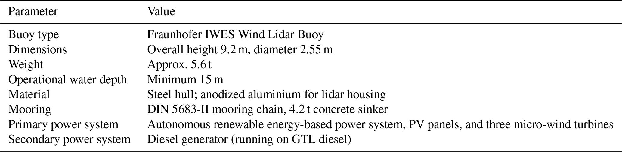
Due to its design and mooring characteristics, the Fraunhofer IWES Wind Lidar Buoy moves slowly in response to sea motion, effectively dampening wave-induced motions. This results in gradual periodic movements rather than rapid displacements, helping to reduce high-frequency motion influences in lidar measurements while reducing the requirements on motion data precision and time synchronization. However, as the buoy is experiencing motion in all 6 degrees of freedom (see Fig. 1b), periodic variations are introduced in the lidar LoS measurements. These motion effects must be carefully accounted for through motion-compensation algorithms to ensure the accuracy of TI measurements.

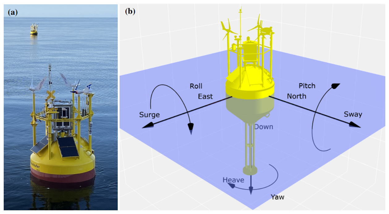
Figure 1 (a) Photograph of the Fraunhofer IWES Wind Lidar Buoy (© Christian Tietjen, Fraunhofer IWES). In panel (b), a schematic representation of the Fraunhofer IWES Wind Lidar Buoy with the IMU's East-North-Down reference coordinate system and arrows denoting the 6 degrees of freedom is depicted.

2.1.2 Vertical profiling wind lidar technologies

In this study, two types of vertical profiling wind lidars were installed in the buoys and studied with respect to the impact of motion on FLS TI measurements: the ZX Lidars ZX300M cw and the Vaisala WindCube V2.1 pulsed lidar system. The measurement principle of each lidar type is illustrated in Fig. 2. The scan pattern of the cw lidar is depicted in (a), while (b) shows that of the pulsed lidar.

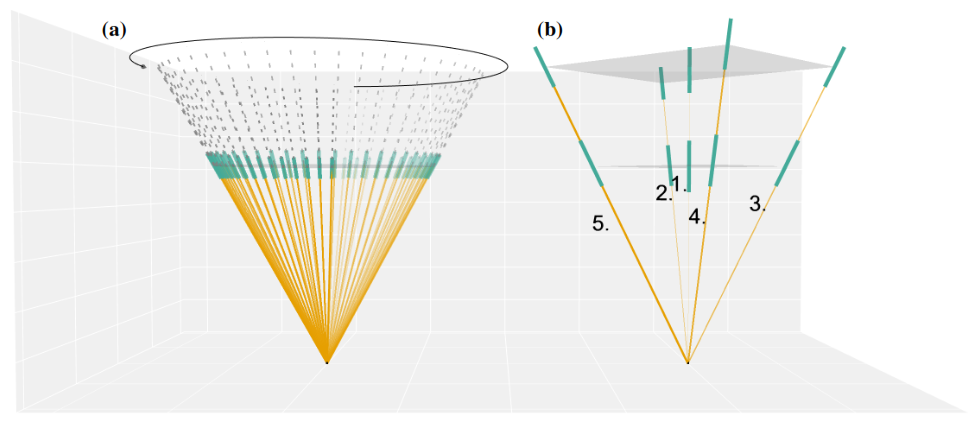
Figure 2 Representation of vertical profiling wind lidar scanning patterns. (a) illustrates the scanning geometry of a cw lidar performing a conical scan at 100 m; (b) depicts the scanning geometry of a pulsed lidar, measuring at two heights simultaneously: 100 and 150 m.

The ZX300M cw vertical profiling lidar – (a) in Fig. 2 – employs focusing optics to concentrate a continuously emitted light beam at predefined heights, conducting LoS measurements (depicted as yellow lines) in a conical scan pattern (sequence and direction implied by an increasing opacity of the yellow LoS lines and the grey arc arrow). Each scan cycle consists of 50 LoS measurements taken within a 1 s interval at one specific height. From each scan, a virtual wind vector is derived, using the velocity–azimuth display (VAD) method before focusing on the subsequent measurement height. A brief overview of the VAD method and the Doppler beam swinging (DBS) retrieval approach used by the pulsed lidar is provided in Appendix A. The predefined heights are scanned consecutively, and the total number of samples taken at each height within a 10 min interval depends on the number of specified measurement heights. The virtual wind vector is intended to represent the wind conditions over the lidar (grey area), ensuring that the resulting 10 min average time series accurately reflects the wind speed and wind direction as measured by a met mast (cup anemometers and wind vanes). Due to its focusing optics, the probe length of a cw lidar increases with measurement height. The green lines in Fig. 2 imply the probe length for a scan at 100 m (±7.70 m). The ZX300M is based on homodyne detection, which means that only the unsigned absolute value of the Doppler shift can be determined from the LoS measurements. Consequently, it cannot distinguish whether the wind is approaching or moving away, leading to a 180° ambiguity. To mitigate this ambiguity, the system relies on reference wind direction data supplied by an additional met station device typically installed closely above the lidar.

The Vaisala WindCube V2.1 pulsed lidar system – panel (b) in Fig. 2 – sequentially emits light pulses in four equally spaced 90° azimuth beam directions alongside one vertical beam (red lines in Fig. 2). The order of the sequence is marked with numbers as well as decreasing opacity of the yellow LoS lines. This scanning pattern is similar to a VAD and is often referred to as DBS. The time elapsed from the emission of each pulse is utilized to calculate the distance travelled by the light, thereby determining the measurement heights, referred to as range gates. The backscattered signal within each range gate is collected, and the LoS velocity is derived. From these LoS measurements, virtual wind vectors are calculated using the DBS method to represent the wind conditions at the corresponding height above the lidar (grey areas). The probe length of a pulsed lidar stays constant along all measurement heights. The green lines imply the probe length for a scan at 100 and 150 m (26.25 m). The WindCube V2.1 deployed in this study was configured to collect LoS data at an increased effective scanning frequency of 5 Hz to better resolve the dominant motion and turbulence timescales, compared to the standard 1 Hz configuration.

2.1.3 FINO3 offshore met mast

The Forschungsplattform in Nord- und Ostsee 3 (FINO3) met mast is built on a monopile foundation that supports a platform and mast structure. The platform is located west of the DanTysk offshore wind farm, as shown in Fig. 4. The mast cross-section varies with height, which can result in stronger mast blockage effects at lower measurement altitudes (FINO3 Research Platform, 2024). FINO3 provides reference wind speed measurements at multiple heights using cup and sonic anemometers (refer to Table 2). For this study, only cup anemometers that are mounted on booms with the same orientation (345° N) are selected, allowing the use of the same free-inflow sector for all altitudes. Wind vanes for measuring wind direction are located at heights of 29 and 101 m.

2.2 Floating lidar motion compensation

The deterministic motion-compensation algorithm applied in this study builds upon the approach of Wolken-Möhlmann et al. (2010, 2014), which accounts for tilted and rotated LoS beam vectors and for translational velocities induced by surge, sway, and heave. In the present implementation, the method is extended to also include angular velocities from tilt motions, as well as the change in effective measurement height caused by heave and tilt.

A cw or pulsed lidar scan consists of multiple beams, each associated with a specific timestamp t_i. Each beam measures the wind velocity component along its pointing direction – referred to as the LoS or radial velocity. For beam i, the lidar returns a scalar value of ν_LoS(t_i), which represents the projection of the three-dimensional wind vector u(t_i) onto the beam's unit direction vector ${\widehat{\mathit{v}}}_i\left(t_i\right)$. This projection is given by the dot product

$$\begin{array}{}\text{(1)}& {\widehat{\mathit{v}}}_i\left(t_i\right)\cdot \mathit{u}\left(t_i\right)={\mathit{\nu }}_{\text{LoS}}\left(t_i\right).\end{array}$$

Each lidar scan consists of N beams. The unit vectors of these beams in the lidar's local coordinate system are described by the matrix $\widehat{\mathbf{V}}\in {\mathbb{R}}^{N\times \mathrm{3}}$, whose rows are the unit vectors ${\widehat{\mathit{v}}}_i\left(t_i\right)$. These vectors are derived from the beam-specific azimuth angle θ_i(t_i) and a fixed half-cone opening angle α, and represent the line-of-sight directions relative to the lidar frame:

$$\begin{array}{}\text{(2)}& \widehat{\mathbf{V}}(t_{\mathrm{1}},\mathrm{\dots },t_N)=\left[\begin{array}{ccc}\sin \left(\mathit{\alpha }\right)\cos \left({\mathit{\theta }}_{\mathrm{1}}\right(t_{\mathrm{1}}\left)\right)& \sin \left(\mathit{\alpha }\right)\sin \left({\mathit{\theta }}_{\mathrm{1}}\right(t_{\mathrm{1}}\left)\right)& \cos \left(\mathit{\alpha }\right)\\ \sin \left(\mathit{\alpha }\right)\cos \left({\mathit{\theta }}_{\mathrm{2}}\right(t_{\mathrm{2}}\left)\right)& \sin \left(\mathit{\alpha }\right)\sin \left({\mathit{\theta }}_{\mathrm{2}}\right(t_{\mathrm{2}}\left)\right)& \cos \left(\mathit{\alpha }\right)\\ \mathrm{⋮}& \mathrm{⋮}& \mathrm{⋮}\\ \sin \left(\mathit{\alpha }\right)\cos \left({\mathit{\theta }}_N\right(t_N\left)\right)& \sin \left(\mathit{\alpha }\right)\sin \left({\mathit{\theta }}_N\right(t_N\left)\right)& \cos \left(\mathit{\alpha }\right)\end{array}\right].\end{array}$$

To express these beam directions in the global coordinate system, we apply a standard rotation matrix of $\mathbf{R}\left(t_i\right)\in {\mathbb{R}}^{\mathrm{3}\times \mathrm{3}}$, which is computed from the roll, pitch, and yaw angles at timestamp t_i. The individual rotation matrices are defined as R_roll(t_i), R_pitch(t_i), and R_yaw(t_i). The combined rotation matrix at time t_i is then given by

$$\begin{array}{}\text{(3)}& \mathbf{R}\left(t_i\right)={\mathbf{R}}_{\text{yaw}}\left(t_i\right){\mathbf{R}}_{\text{pitch}}\left(t_i\right){\mathbf{R}}_{\text{roll}}\left(t_i\right).\end{array}$$

Each beam vector is individually transformed into the global reference frame as

$$\begin{array}{}\text{(4)}& {\widehat{\mathit{v}}}_i^{\text{rot}}\left(t_i\right)={\widehat{\mathit{v}}}_i\left(t_i\right)\mathbf{R}(t_i{)}^{\top },i=\mathrm{1},\mathrm{\dots },N,\end{array}$$

resulting in the rotated matrix

$$\begin{array}{}\text{(5)}& {\widehat{\mathbf{V}}}_{\text{rot}}=\left[\begin{array}{c}{\widehat{\mathit{v}}}_{\mathrm{1}}^{\text{rot}}\left(t_{\mathrm{1}}\right)\\ {\widehat{\mathit{v}}}_{\mathrm{2}}^{\text{rot}}\left(t_{\mathrm{2}}\right)\\ \mathrm{⋮}\\ {\widehat{\mathit{v}}}_N^{\text{rot}}\left(t_N\right)\end{array}\right]\in {\mathbb{R}}^{N\times \mathrm{3}}.\end{array}$$

On a platform in motion, the measured LoS velocity is a combination of the wind-induced velocity and the platform's motion projected along the same direction. To account for this, the platform motion must be considered.

At each timestamp t_i, the translational velocity of the lidar platform in the global coordinate system is given by

$$\begin{array}{}\text{(6)}& {\mathit{u}}_{\text{motion}}\left(t_i\right)=\left[\begin{array}{c}{u}_{\text{surge}}\left(t_i\right)\\ v_{\text{sway}}\left(t_i\right)\\ w_{\text{heave}}\left(t_i\right)\end{array}\right],\end{array}$$

where the components represent motion in the forward (surge), lateral (sway), and vertical (heave) directions, respectively. If the lidar is mounted above the platform's tilting point, pitch and roll can introduce additional motion at the lidar location due to the lever arm effect. In such cases, the angular velocity should be taken into account when computing the full translational velocity of the lidar.

This motion introduces an additional component to the measured LoS velocity in beam i, which is computed as the projection of u_motion(t_i) onto the corresponding rotated beam direction ${\widehat{\mathit{v}}}_i^{\text{rot}}\left(t_i\right)$:

$$\begin{array}{}\text{(7)}& {\mathit{\nu }}_{\text{motion}}\left(t_i\right)={\widehat{\mathit{v}}}_i^{\text{rot}}\left(t_i\right)\cdot {\mathit{u}}_{\text{motion}}\left(t_i\right).\end{array}$$

This velocity must be considered to isolate the wind-induced component

$$\begin{array}{}\text{(8)}& {\mathit{\nu }}_{\text{LoS, corr}}\left(t_i\right)={\mathit{\nu }}_{\text{LoS}}\left(t_i\right)-{\mathit{\nu }}_{\text{motion}}\left(t_i\right).\end{array}$$

Assuming the wind vector u(t)∈ℝ³ is constant during the scan, we can estimate it from the N rotated unit vectors and the corresponding LoS velocities. For N>3, the system is overdetermined and can be solved using the least-squares approach:

$$\begin{array}{}\text{(9)}& \left[\begin{array}{ccc}{\widehat{v}}_{\mathrm{1}x}^{\text{rot}}\left(t_{\mathrm{1}}\right)& {\widehat{v}}_{\mathrm{1}y}^{\text{rot}}\left(t_{\mathrm{1}}\right)& {\widehat{v}}_{\mathrm{1}z}^{\text{rot}}\left(t_{\mathrm{1}}\right)\\ {\widehat{v}}_{\mathrm{2}x}^{\text{rot}}\left(t_{\mathrm{2}}\right)& {\widehat{v}}_{\mathrm{2}y}^{\text{rot}}\left(t_{\mathrm{2}}\right)& {\widehat{v}}_{\mathrm{2}z}^{\text{rot}}\left(t_{\mathrm{2}}\right)\\ \mathrm{⋮}& \mathrm{⋮}& \mathrm{⋮}\\ {\widehat{v}}_{Nx}^{\text{rot}}\left(t_N\right)& {\widehat{v}}_{Ny}^{\text{rot}}\left(t_N\right)& {\widehat{v}}_{Nz}^{\text{rot}}\left(t_N\right)\end{array}\right]\left[\begin{array}{c}u\left(t\right)\\ v\left(t\right)\\ w\left(t\right)\end{array}\right]=\left[\begin{array}{c}{\mathit{\nu }}_{\text{LoS, corr}}\left(t_{\mathrm{1}}\right)\\ {\mathit{\nu }}_{\text{LoS, corr}}\left(t_{\mathrm{2}}\right)\\ \mathrm{⋮}\\ {\mathit{\nu }}_{\text{LoS, corr}}\left(t_N\right)\end{array}\right].\end{array}$$

In the case of a cw lidar performing a conical scan at a fixed elevation angle, the beam geometry matches the assumptions of the classical VAD method, which assumes horizontal homogeneity during the scan. It can similarly be applied to pulsed lidars, in this case operating in a five-beam DBS configuration.

Following the same principle as in Fig. 2, Fig. 3 visualizes extreme events of tilted LoS beam vectors of a floating cw lidar (a) and a floating pulsed lidar (b) from actual measurement data.

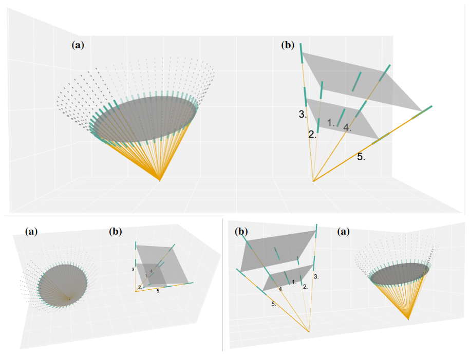
Figure 3 Simulation of tilted vertical profiling wind lidar measurement principles. Panel (a) illustrates the scanning geometry of a cw lidar performing a conical scan at 100 m; panel (b) depicts the scanning geometry of a pulsed lidar, measuring at two heights simultaneously: 100 and 150 m.

As shown in Fig. 3, the tilting, yawing, and heave directly influence the scanning geometry of the lidar systems, deforming the scan volume. The changed measurement height (due to tilt and heave) is considered in different ways, depending on the lidar type. As pulsed lidar systems take measurements almost simultaneously (see Sect. 2.1.2) at multiple heights, the LoS velocity of each beam can be interpolated to the desired measurement height by considering adjacent measurements from neighbouring heights of the same pulse. Cw lidars conduct sequential measurements, focusing on one measurement height before progressing to the next. Consequently, the interpolation method is not applicable. To account for changes in measurement height, the power law wind profile (IEC, 2019) is applied to the radial wind velocity of each transformed LoS. After applying the transformation matrices to the LoS beams and compensating the measured radial velocities for the motion as described, the virtual wind vector is calculated by applying the VAD or DBS method, depending on the instrument.

Potential time offsets between the lidar and the motion-sensor data are identified by repeating the motion compensation several times for each 10 min interval, while shifting the lidar data by small time increments (time offsets). The standard deviation of each resulting 10 min wind interval is determined, and the interval with the lowest standard deviation is selected. A lower standard deviation indicates less fluctuation and, consequently, a reduced influence of motion on the measured wind data. The corresponding time offset then becomes the basis for the offset iteration of the next 10 min interval. Depending on the lidar type, the time offset increases over time until the device re-synchronizes, at which point the time offset returns to zero. To consider this re-synchronization, the time-offset iteration always includes a time offset of zero.

2.3 Performance assessment metrics

In this subsection, we introduce the performance assessment metrics used to evaluate the TI measurements. Building on the wind industry's standard practice of analysing 10 min statistical intervals, we derive time series data that can be statistically analysed, for example, through linear regression. For standard parameters, such as mean wind speed and direction, this approach yields the slope, offset, and R², for which KPIs are defined in The Carbon Trust (2018). A similar methodology can be applied to TI, while alternative metrics might be more directly connected to the application of TI.

We begin by describing the application of the linear regression techniques in Sect. 2.3.1 to capture the overall trend between the TI measurements. Section 2.3.2 then introduces the mean bias error and mean relative bias error, which are used to quantify systematic differences between the datasets. In Sect. 2.3.3, we describe the calculation of the root mean square error and its normalized variant (relative root mean square error), which highlight the magnitude of random error or precision. Section 2.3.4 focuses on the representative TI error, derived from the 90th percentile of the TI distribution. Finally, Sect. 2.3.5 presents a quantile-based distribution analysis that provides a visual assessment of measurement distributions and potential biases.

2.3.1 Linear regression

Linear regression and correlation analysis are commonly used to compare wind speed and wind direction measurements from multiple sources, such as in calibration campaigns or for plausibility checks of data. While OLS assumes that all measurement errors are confined to the dependent variable, Deming regression accounts for uncertainties in both the independent and dependent variables. In this study, we will investigate the performance using OLS, RTO, and Deming regression for comparison. While the uncentred R² is recommended for RTO, it has been observed to produce abnormally high values, which distort the results. The uncentred R² ($R_{\mathrm{uncentered}}^{\mathrm{2}}$) is described as follows:

$$\begin{array}{}\text{(10)}& R_{\mathrm{uncentered}}^{\mathrm{2}}=\mathrm{1}-{\displaystyle \frac{{\sum }_{n=\mathrm{1}}^N{\left({\mathrm{TI}}_{\mathrm{ref},n}-{\mathrm{TI}}_{\mathrm{comp},n}\right)}^{\mathrm{2}}}{{\sum }_{n=\mathrm{1}}^N{\left({\mathrm{TI}}_{\mathrm{ref},n}\right)}^{\mathrm{2}}}},\end{array}$$

where TI_comp is the comparison quantity, TI_ref is the reference quantity, n refers to the individual data point, and N is the total number of data points.

To calculate R², we will use the following equation as an alternative to the uncentred R²:

$$\begin{array}{}\text{(11)}& R^{\mathrm{2}}=\mathrm{1}-{\displaystyle \frac{{\sum }_{n=\mathrm{1}}^N{\left({\mathrm{TI}}_{\mathrm{ref},n}-{\mathrm{TI}}_{\mathrm{comp},n}\right)}^{\mathrm{2}}}{{\sum }_{n=\mathrm{1}}^N{\left({\mathrm{TI}}_{\mathrm{ref},n}-{\stackrel{\mathrm{‾}}{\mathrm{TI}}}_{\mathrm{ref}}\right)}^{\mathrm{2}}}}.\end{array}$$

Using this equation, R² might yield negative values when the predictions are worse than simply using the mean of the observed data as a predictor. In that case, we will print “not a number” (NaN).

2.3.2 Mean bias error and mean relative bias error

The TI MBE as a function of binned wind speed is defined as follows (St. Pé et al., 2021):

$$\begin{array}{}\text{(12)}& {\mathrm{TI}}_{\mathrm{MBE},i}={\displaystyle \frac{\mathrm{1}}{N_i}}\sum _{n=\mathrm{1}}^{N_i}{\mathrm{TI}}_{\mathrm{comp},n,i}-{\mathrm{TI}}_{\mathrm{ref},n,i},\end{array}$$

where i is the wind speed bin (with a bin size of 1 m s⁻¹) and N_i is the number of data points in the ith bin. The TI MBE measures the average difference between two datasets, helping to identify any consistent deviations. It reveals systematic over- and underestimations (bias), thus indicating the direction of the error.

The TI MRBE, as introduced by DNV (2023), is deployed to derive the relative error (relative TI bias) between lidar and cup anemometer TI. It is a variation of the mean bias error that expresses bias as a normalized measure. It is defined as follows:

$$\begin{array}{}\text{(13)}& {\mathrm{TI}}_{\mathrm{MRBE},i}={\displaystyle \frac{\mathrm{1}}{N_i}}\sum _{n=\mathrm{1}}^{N_i}{\displaystyle \frac{({\mathrm{TI}}_{\mathrm{comp},n,i}-{\mathrm{TI}}_{\mathrm{ref},n,i})}{{\mathrm{TI}}_{\mathrm{ref},n,i}}}\times \mathrm{100}.\end{array}$$

The metric again reveals systematic over- and underestimations but by normalizing the bias, the error becomes easier to interpret.

2.3.3 Root mean square error and relative root mean square error

The TI RMSE as a function of binned wind speed is denoted as follows (St. Pé et al., 2021):

$$\begin{array}{}\text{(14)}& {\mathrm{TI}}_{\mathrm{RMSE},i}=\sqrt{{\displaystyle \frac{\mathrm{1}}{N_i}}\sum _{n=\mathrm{1}}^{N_i}({\mathrm{TI}}_{\mathrm{comp},n,i}-{\mathrm{TI}}_{\mathrm{ref},n,i}{)}^{\mathrm{2}}}.\end{array}$$

The TI RMSE quantifies the magnitude of random errors between two datasets by calculating the square root of the average squared differences. By focusing on squared differences, it highlights the random errors and statistical variability that may arise due to differences in measurement instruments.

Normalizing the TI RMSE yields the TI RRMSE that enables direct comparisons across different datasets. It is defined as follows (DNV, 2023):

$$\begin{array}{}\text{(15)}& {\mathrm{TI}}_{\mathrm{RRMSE},i}=\sqrt{{\displaystyle \frac{\mathrm{1}}{N_i}}\sum _{n=\mathrm{1}}^{N_i}{\left({\displaystyle \frac{({\mathrm{TI}}_{\mathrm{comp},n,i}-{\mathrm{TI}}_{\mathrm{ref},n,i})}{{\mathrm{TI}}_{\mathrm{ref},n,i}}}\right)}^{\mathrm{2}}}\times \mathrm{100}.\end{array}$$

2.3.4 Representative TI error

The representative TI is defined as the 90th quantile (Q90) of a TI dataset. For Gaussian distributions, the Q90 can be approximated according to St. Pé et al. (2021):

$$\begin{array}{}\text{(16)}& {\mathrm{TI}}_{\mathrm{Rep},i}={\mathrm{TI}}_{\mathrm{avg},i}+\mathrm{1.28}\times {\mathrm{TI}}_{\mathrm{std},i},\end{array}$$

where TI_avg is the average TI and TI_std is the standard deviation of the TI.

We also apply this equation in our study, instead of calculating the Q90 based on the data population per bin. The representative TI error is the difference between the binned representative TI values of the reference and the trialled system:

$$\begin{array}{}\text{(17)}& {\mathrm{TI}}_{{\mathrm{Rep}}_{\mathrm{error}},i}={\displaystyle \frac{\mathrm{1}}{N_i}}\sum _{n=\mathrm{1}}^{N_i}({\mathrm{TI}}_{\mathrm{Rep},\mathrm{comp},i}-{\mathrm{TI}}_{\mathrm{Rep},\mathrm{ref},i}).\end{array}$$

2.3.5 Quantile-based distribution analysis

A Q–Q analysis is a graphical tool used to compare the distributions of datasets by plotting their quantiles against each other. It helps to assess the goodness of fit between datasets, allowing for the visual identification of whether the data follow the reference distribution or show patterns of systematic error or outliers. Additionally, overestimation and underestimation (systematic bias) can be derived from the plot by examining the position of the data points relative to the 1:1 line.

2.4 Campaign details

Two FLSs of the type Fraunhofer IWES Wind Lidar Buoy were deployed in proximity to the FINO3 offshore met mast from 6 March 2024 to 3 August 2024. The distance between the FLSs and the met mast was approximately 300 m. One FLS was equipped with a ZX Lidars ZX300M cw lidar system (FLS ZX), the other one with a Vaisala WindCube V2.1 pulsed lidar in a 5 Hz scanning configuration (FLS WC). Additionally, a ZX Lidars ZX300M cw lidar system (fixed ZX) was installed on the FINO3 met mast platform at a height of approximately 27 m above the lowest astronomical tide (LAT). Both cw lidar systems were running the same firmware version (v3.3002).

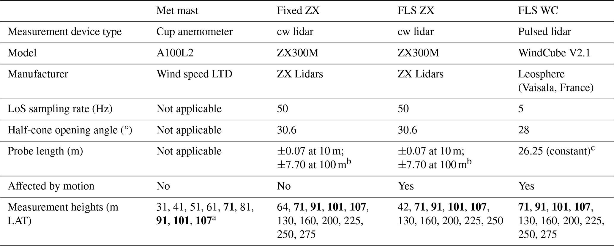
An overview of the device characteristics and configurations is given in Table 2.

Table 2 Measurement device characteristics. Matching wind speed measurement heights are marked in bold.

^a FINO3 Research Platform (2024); ^b ZX Lidars (2024); ^c Calculated according to Eq. (29) in Peña (2009).

The positions of all systems are shown in Fig. 4.

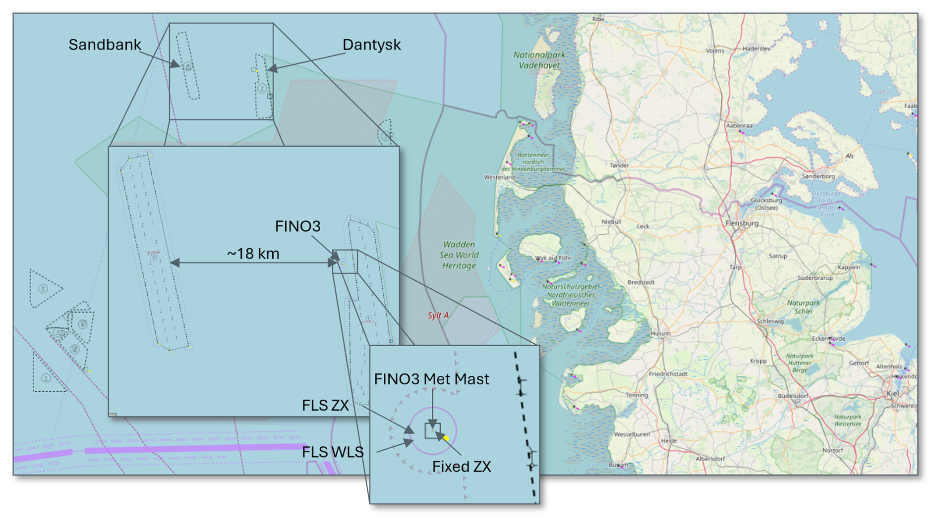
Figure 4 Measurement campaign location at FINO3 in the German North Sea (based on OpenSeaMap Data (© OpenSeaMap, 2025) under the Open Database License (ODbL)).

To enhance the accuracy of the motion-compensation results, the settings of the motion sensors deployed on the FLS were optimized on 6 April 2024. The fixed cw lidar installed on the FINO3 met mast platform (fixed ZX) stopped recording data due to a power supply failure on 9 July 2024; as a result, only data recorded from 6 April to 9 July were considered in this study.

Additionally, only timestamps where data from all measurement systems were available were considered. A wind sector filter is applied to only consider wind data coming from the free-inflow sector at 220 to 300°, using the FINO3 met mast wind vane installed at 101 m above LAT as reference.

The met mast and wave radac reference datasets were obtained from the BSH Insitu database (, ). All entries that were flagged as questionable or bad by the database providers were removed from the analysis. Only timestamps where all systems recorded data were considered in the analysis. Within that period, a range of environmental conditions were covered, with average wind speeds reaching up to 26.54 m s⁻¹ (measured by the cup at 101 m), significant wave heights (H_s) reaching up to 4.28 m, and peak wave periods (T_p) of up to 12.5 s.

No data were recorded by the cup anemometer mounted at 91 m. Furthermore, a data gap is present in the radac H_s and T_p records from 7 June 2024, 09:00:00 to 19 June 2024, 07:50:00 UTC, which may affect the statistics of certain sea state parameters, shown in Fig. 5. Panel (a) displays a wind rose, illustrating the distribution of wind directions recorded by the wind vane at 101 m LAT, along with the corresponding bin-wise wind speed distribution measured by the cup anemometer at the same height. Panel (b) presents a density correlation plot of significant wave height versus spectral peak period measured by the radac mounted on the met mast.

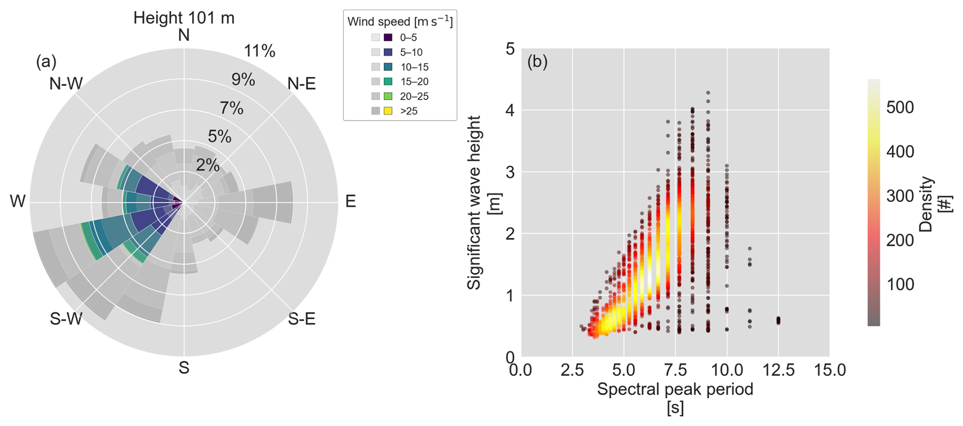
Figure 5 Statistical overview of reference conditions recorded during the trial period: (a) wind rose displaying wind direction distribution measured by the wind vane at 101 m LAT, along with the corresponding bin-wise wind speed distribution from the cup anemometer at the same height (grey scales correspond to the whole campaign period, while blue/green scales represent the selected timestamps); (b) significant wave height versus spectral peak period density correlation plot measured by the radac mounted on the met mast.

3 Results

This section evaluates the TI data recorded during the measurement campaign, focusing on how two lidar types – cw (represented by a ZX Lidars ZX300M) and pulsed (represented by a Vaisala WindCube V2.1) – perform with and without motion compensation. For results on the mean horizontal wind speed, please refer to Appendix B. Both systems were deployed on FLS platforms of the same type, operated under similar offshore conditions and compensated using the same deterministic algorithm, enabling the effect of lidar type to be isolated. The resulting TI measurements are validated against met mast cup anemometer data and cross-checked with a fixed cw lidar to evaluate motion-compensation effectiveness and relative system performance. All pulsed lidar results presented here correspond to the 5 Hz effective scan frequency configuration. This trial represents the first published offshore deployment of a pulsed FLS operating at 5 Hz with full deterministic motion compensation. Previous analyses have shown that a 1 Hz configuration is insufficient in capturing the relevant turbulent timescales for reliable compensation. For completeness, results from a 1 Hz pulsed lidar deployment conducted during a separate campaign at FINO3, including the prevailing sea state, are provided in Appendix C. The results are structured as follows: first, in Sect. 3.1, a correlation analysis is conducted to compare the TI measured by the FLS before and after motion compensation. This is followed by an assessment of systematic deviations through MBE and MRBE in Sect. 3.2. After that, in Sect. 3.3, precision metrics, namely RMSE and RRMSE, are evaluated. Additionally, the representative TI error is examined in Sect. 3.4. Finally, in Sect. 3.5, a quantile-based distribution analysis is conducted to provide further insights into the distribution of FLS TI before and after motion compensation.

To ensure consistency in the analysis, a wind sector filter for the range of 220 to 300° was applied, based on wind direction data from the met mast wind vane at 101 m above LAT. Additionally, for the regression analysis and the quantile-based distribution analysis, only wind speed data in the range of 4 to 16 m s⁻¹, as measured by the met mast cup anemometer at the same height, were considered. The results presented in this section are based on measurements from 101 m above LAT. To test vertical consistency, additional measurement heights (71 and 107 m) were investigated. As the results were consistent with those at 101 m and did not provide further insights, they are not included in this work.

3.1 Linear regression and correlation analysis

For this study, the fixed cw lidar (fixed ZX) TI serves as the baseline for a lidar-derived TI measurement without the influence of motion. This baseline sets the benchmark for assessing the performance of the applied motion-compensation algorithm.

Figure 6 presents a correlation plot comparing fixed cw lidar TI with met mast cup anemometer (MM) TI at 101 m above LAT. To highlight the distribution of data points, the scatter is represented as a density plot, where point density is indicated by a colour scale. A solid black 1:1 line represents perfect agreement between the two measurements. As mentioned in Sect. 2.3.1, three regression models are analysed, with R² calculated according to Eq. (11): OLS regression (dashed red line), RTO (solid red line), and Deming regression (dashed black line). The regression parameters (slope, offset, and R² values) are listed in Table 3 for reference.

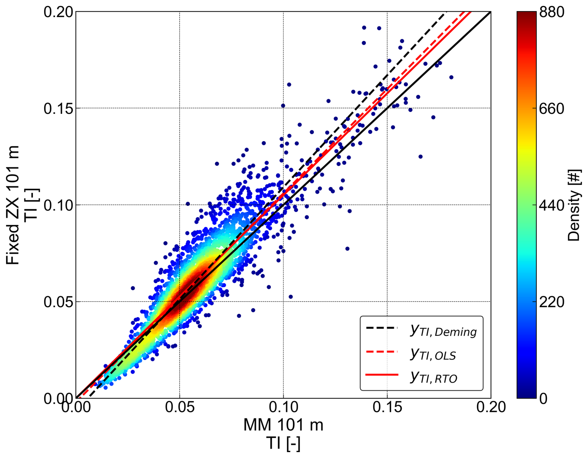
Figure 6 Density correlation plot and regression analysis of the fixed cw lidar (fixed ZX) TI versus the met mast cup anemometer (MM) TI at 101 m above LAT. The point density is indicated by the colour bar. Derived parameters are listed in Table 3.

Table 3 Regression parameters for the correlation between TI measured by the fixed cw lidar (fixed ZX) and the met mast cup anemometer (MM) at 101 m above LAT, as illustrated in Fig. 6.

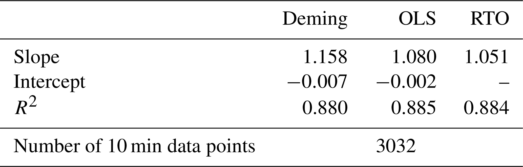
The data points are well aligned along the 1:1 line, indicating a strong correlation between the fixed cw lidar and the met mast cup measurements. All three regression models yield R² values above 0.8. While wind speed and wind direction correlations typically exhibit even higher R² values, this is considered high for a TI correlation. However, a slight overestimation of TI by the fixed cw lidar can be observed, particularly at higher values. The applied regression models confirm this trend with consistent slopes above unity and only minor offsets. Further, the resulting Deming regression slope is higher than the slopes from OLS and RTO, indicating that the cw lidar measurements systematically show higher TI values than the met mast cup reference. As mentioned in Sect. 2.3, the outcome of a regression analysis for TI is significantly influenced by several factors. These include the type and configuration of the measurement device, each of which might have different spatial and temporal resolutions. Additionally, a varying measurement volume between instruments may lead to different sensitivities. The spatial separation between devices introduces further uncertainty, especially in inhomogeneous flow conditions. Although the fixed cw lidar is installed on the met mast platform, the visible scatter, as well as the slope and R² of the three types of regression fits between the two instruments, reveal deviations between the datasets. These discrepancies are primarily caused by the differing underlying measurement principles of the instruments. While lidars are commonly expected to report lower TI values than cup anemometers, the regression slope shows a slight overestimation. We have observed similar behaviour in other offshore datasets involving fixed cw as well as pulsed lidars at FINO3 (the platform) and believe this may be due to site-specific influences such as atmospheric stability conditions or flow disturbances related to the mast structure and layout.

Building on the baseline analysis in Fig. 6, we now compare motion-affected cw lidar data from the FLS (FLS ZX) at 101 m above LAT to the fixed cw lidar TI at the same height. Figure 7 presents two scatter plots, following the same approach as in Fig. 6, with (a) showing the raw (uncorrected) FLS measurements, while (b) displays the motion-compensated results. The corresponding regression parameters are listed in Table 4. As the floating lidar is subject to wave-induced motion, additional velocity fluctuations are introduced, leading to an overestimation of TI compared to the fixed cw lidar. By comparing raw and motion-compensated FLS data, we assess the extent of motion-induced bias and evaluate the effectiveness of the applied correction algorithm in mitigating these effects.

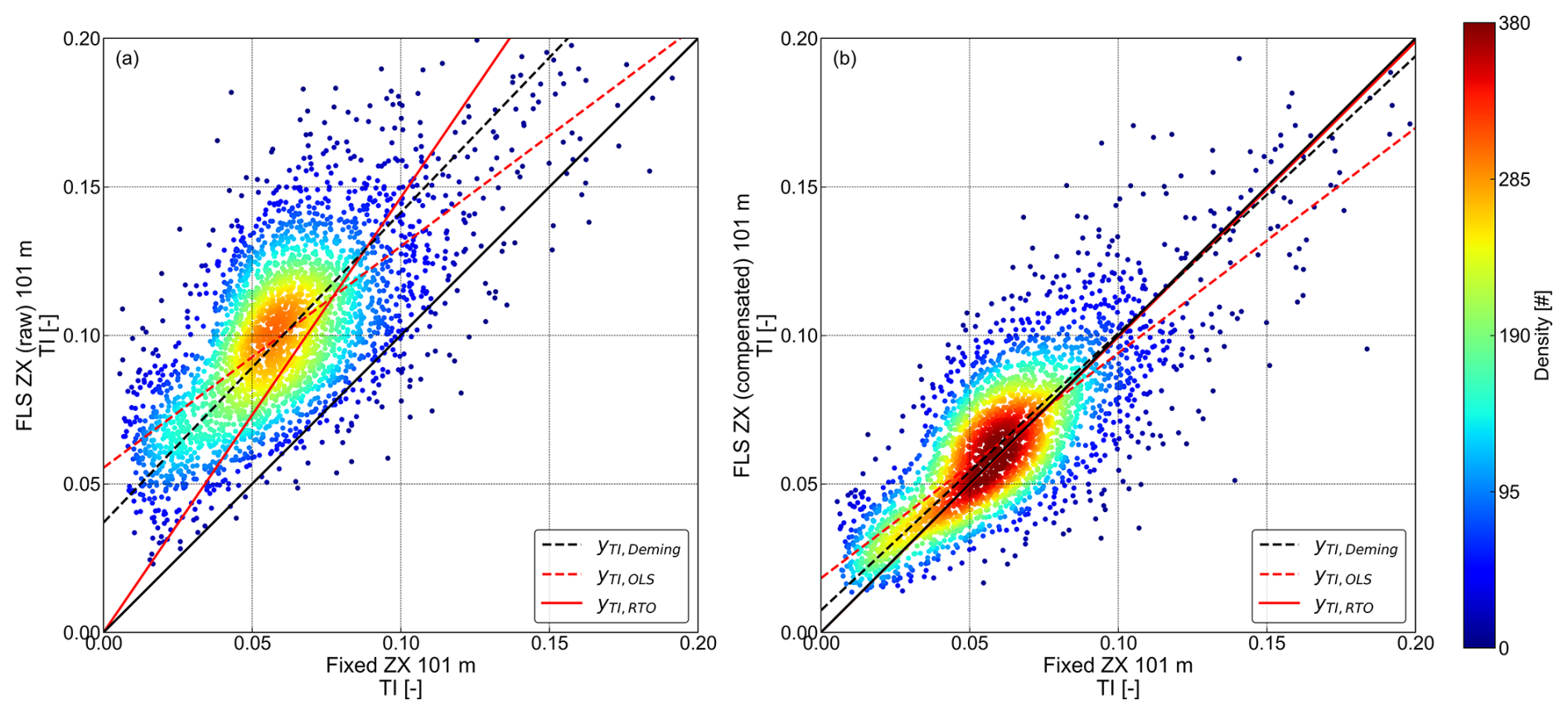
Figure 7 Density correlation plots and regression analyses of TI measured by the floating cw lidar (FLS ZX) versus the fixed cw lidar (fixed ZX) at 101 m above LAT. Panel (a) shows uncompensated (raw) data, while panel (b) shows motion-compensated data. Point density in both panels is indicated by the colour bar. Derived parameters are listed in Table 4.

Table 4 Regression parameters for the correlation between TI measured by the floating cw lidar (FLS ZX) and the fixed cw lidar (fixed ZX) at 101 m above LAT, as illustrated in Fig. 7.

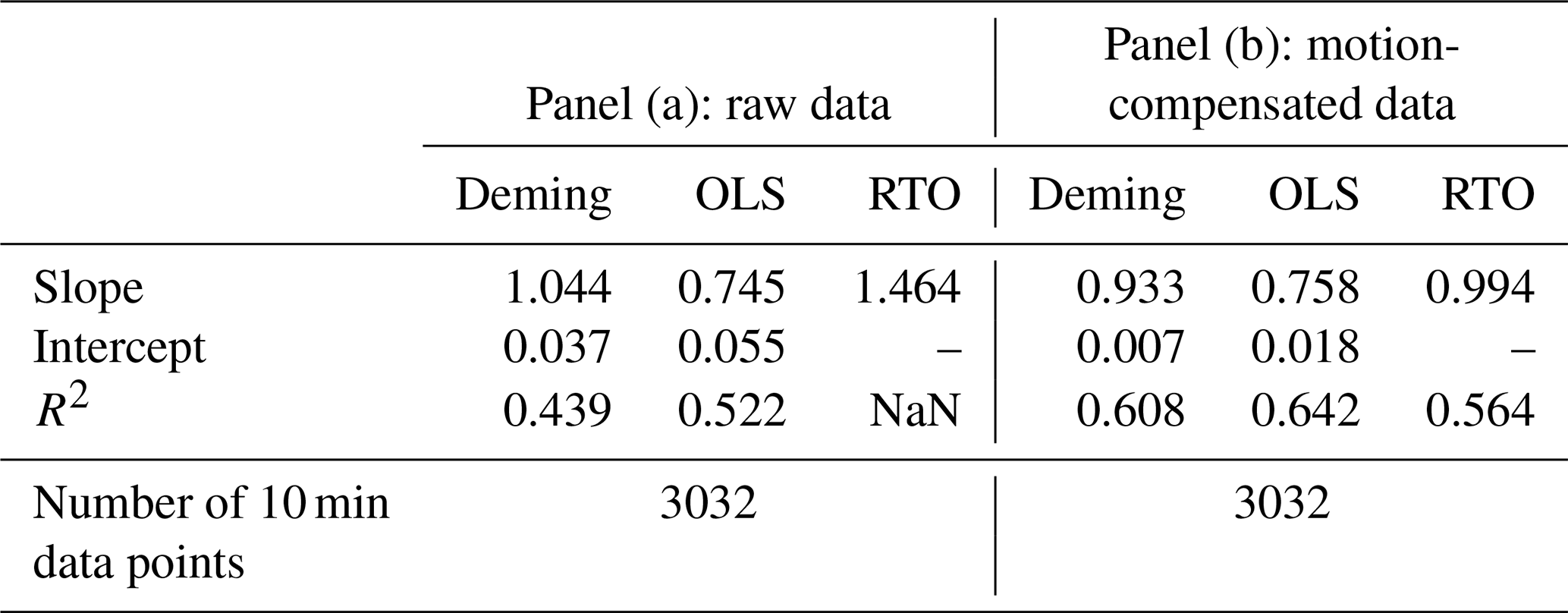
Figure 7 visualizes the difference between the raw (a) and motion-compensated (b) FLS TI measurements.

In panel (a), a noticeable scatter and deviation from the 1:1 line indicates that the floating lidar systematically overestimates TI. This is reflected in the regression parameters listed in Table 4, where all models show lower R² values compared to the motion-compensated variant in panel (b). In the raw cw FLS data, the Deming regression results in a slope of 1.044 and an offset of 0.037, with an R² of 0.439, indicating a moderate correlation alongside a systematic overestimation reflected in the high offset. The OLS regression produces a much lower slope of 0.745 alongside an offset of 0.055, further suggesting that the raw cw FLS TI measurements tend to diverge significantly from the fixed cw lidar TI. The RTO regression, with a slope of 1.464, suggests a high overestimation, while its negative R² value underlines the poor fit (and is therefore marked as NaN).

After motion compensation (panel b), the scatter is reduced, and the correlation between cw FLS and fixed cw lidar significantly improves across the three analysed regression models. The Deming regression now results in a slope below unity and a minor offset of 0.007, with an increased R² of 0.608, suggesting that the overall overestimation seen in the raw cw FLS data has largely been corrected, leaving a slight overestimation at low TI that transitions to increasing underestimation with higher TI. The OLS regression shows a similar slope as in the raw cw FLS data but with a much lower offset and an increased R², indicating that the motion compensation has not only reduced the bias but also reduced the scatter between the two datasets. The RTO regression, with a slope of 0.994 and an R² of 0.564, now provides a reasonable fit, supporting the improvement of the data quality.

These results confirm that the applied motion-compensation algorithm effectively mitigates the motion-induced overestimation seen in the raw cw FLS TI data. However, the slopes below 1, in combination with an offset, indicate a range-dependent tilt rather than a uniform bias, with slight overestimation at low TI, transitioning to underestimation as TI increases. Several factors contribute to these remaining discrepancies.

To account for translational motion in deterministic LoS motion compensation, each measured LoS velocity is adjusted by adding or subtracting the platform’s translational velocity. This approach depends critically on resolving the correct sign of each LoS. Under conditions of non-uniform flow, especially at low wind speeds and high TI, sign determination becomes challenging due to the homodyne detection method of the trialled cw lidar (ZX Lidars ZX300M) (see Sect. 2.1.2) and the assumption of homogeneous flow in the VAD scanning pattern. If the sign is misidentified, for example, if the wind is actually moving away from the platform but is interpreted as moving towards it, the compensation will apply the opposite adjustment, introducing systematic errors into the derived virtual wind vectors and potentially amplifying motion-induced fluctuations. Further factors are, for example, the remaining time offsets between the IMU and lidar device, poor time stamping precision, the distance between the instruments (see Sect. 2.4), the different probe volumes, and the smaller focal length of the elevated reference lidar compared to the floating cw lidar.

While Fig. 7 has focused on the comparison between the floating and fixed cw lidar TI, the next step has been to investigate whether similar trends are observed for the floating pulsed lidar system (FLS WC). Figure 8 shows one of the main results and key novelties of this study: deterministic motion compensation applied to the floating pulsed lidar (FLS WC) significantly improves TI agreement with the fixed cw lidar at 101 m above LAT. The comparison follows the same approach as in Figs. 6 and 7. Since pulsed lidars differ in their measurement principles, particularly the scanning geometry and range gating (see Sect. 2.1.2), the impact of motion and the effectiveness of the compensation algorithm is expected to show different characteristics compared to the floating cw lidar system.

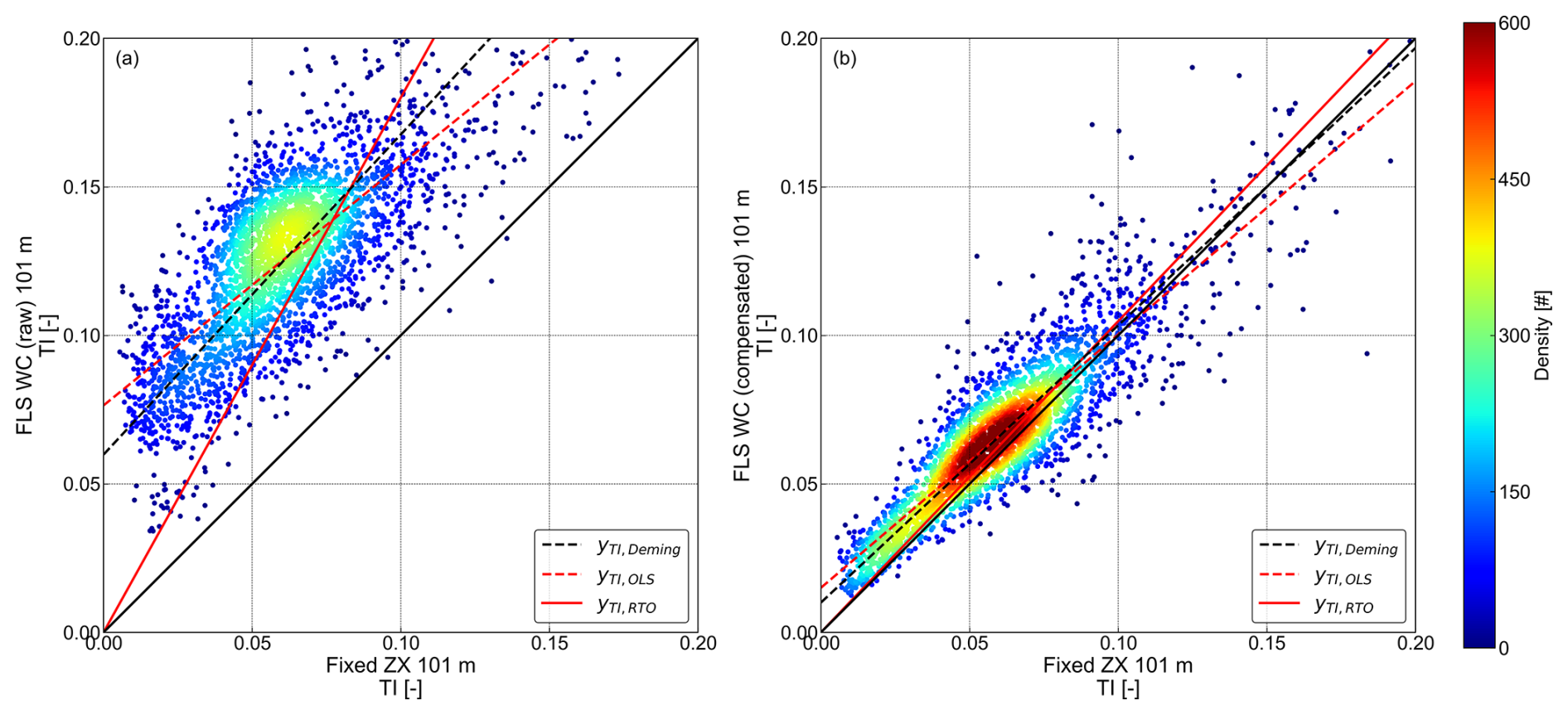
Figure 8 Density correlation plots and regression analyses of TI measured by the floating pulsed lidar (FLS WC) versus the fixed cw lidar (fixed ZX) at 101 m above LAT. Panel (a) shows uncompensated (raw) data, while panel (b) shows motion-compensated data. Point density in both panels is indicated by the colour bar. Derived parameters are listed in Table 5.

Table 5 Regression parameters for the correlation between TI measured by the floating pulsed lidar (FLS WC) and the fixed cw lidar (fixed ZX) at 101 m above LAT, as illustrated in Fig. 8.

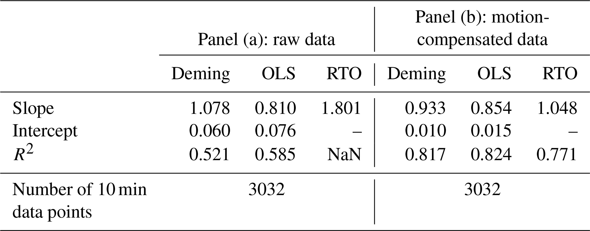
In Fig. 8, the scatter plots reveal distinct differences between the raw (panel a) and motion-compensated (panel b) TI measurements from the floating pulsed lidar (FLS WC). The raw dataset exhibits wide scatter, with data points deviating significantly from the 1:1 line. This increased dispersion, along with a consistent upward shift, suggests a systematic overestimation of TI and highlights the strong influence of platform motion on the floating pulsed lidar measurements.

The regression models further confirm this trend. Deming regression yields a slope of 1.078 with a high offset of 0.060, while OLS regression results in a slope of 0.810 and an even higher offset of 0.076, both reflecting the overestimation. RTO yields a slope of 1.801 with a negative R² underlining the severe overestimation but also revealing the poor fit.

In contrast, the motion-compensated dataset (panel b) exhibits a clear reduction in scatter and overestimation, with data points and regression fits aligning closely with the 1:1 line. This improvement is further reflected in significantly reduced offsets and increased R² values across all models and regression slopes, generally shifting closer to unity. The density scatter plot reveals an overestimation of TI for lower values, tilting the derived slopes. The RTO slope decreases from 1.801 to 1.048, now closely aligning with the 1:1 line. Meanwhile, the Deming regression slope decreases from 1.078 to 0.933, and for OLS it increases from 0.810 to 0.854, while both exhibit a significant reduction in positive offset (0.060 to 0.010 for Deming; 0.076 to 0.015 for OLS). Combined with the sub-unity slopes, this indicates a range-dependent tilt rather than a uniform bias: an overestimation at low TI transitioning towards slight underestimation as TI increases. The overall increase in R² confirms that the compensation algorithm successfully corrects the TI measurements and significantly improves agreement with the fixed cw lidar. The remaining discrepancies may be attributed to similar factors as previously mentioned, with the added influence of the different underlying measurement principles of the compared lidars.

3.2 Mean bias error and mean relative bias error

The figures in Sect. 3.1 demonstrated how the applied deterministic motion compensation reduced scatter and systematic overestimation in floating lidar TI measurements. While the regression analysis provided insights into the overall relationship between the datasets, a more detailed performance assessment is conducted by evaluating systematic deviations and measurement accuracy across different wind speed bins. To achieve this, the following analysis examines further performance assessment metrics, as introduced in Sect. 2.3.

The following Fig. 9 illustrates the binned MBE (calculated according to Eq. (12) in Sect. 2.3.2) between the met mast cup TI and the trialled lidar devices TI as a function of binned wind speed. The figure includes both raw and motion-compensated datasets (where applicable), distinguished by dashed and solid lines, respectively. The x axis represents the wind speed bins, while the y axis displays the corresponding error metric values. The figure also features minimum and best-practice performance thresholds, indicated by dashed horizontal lines.

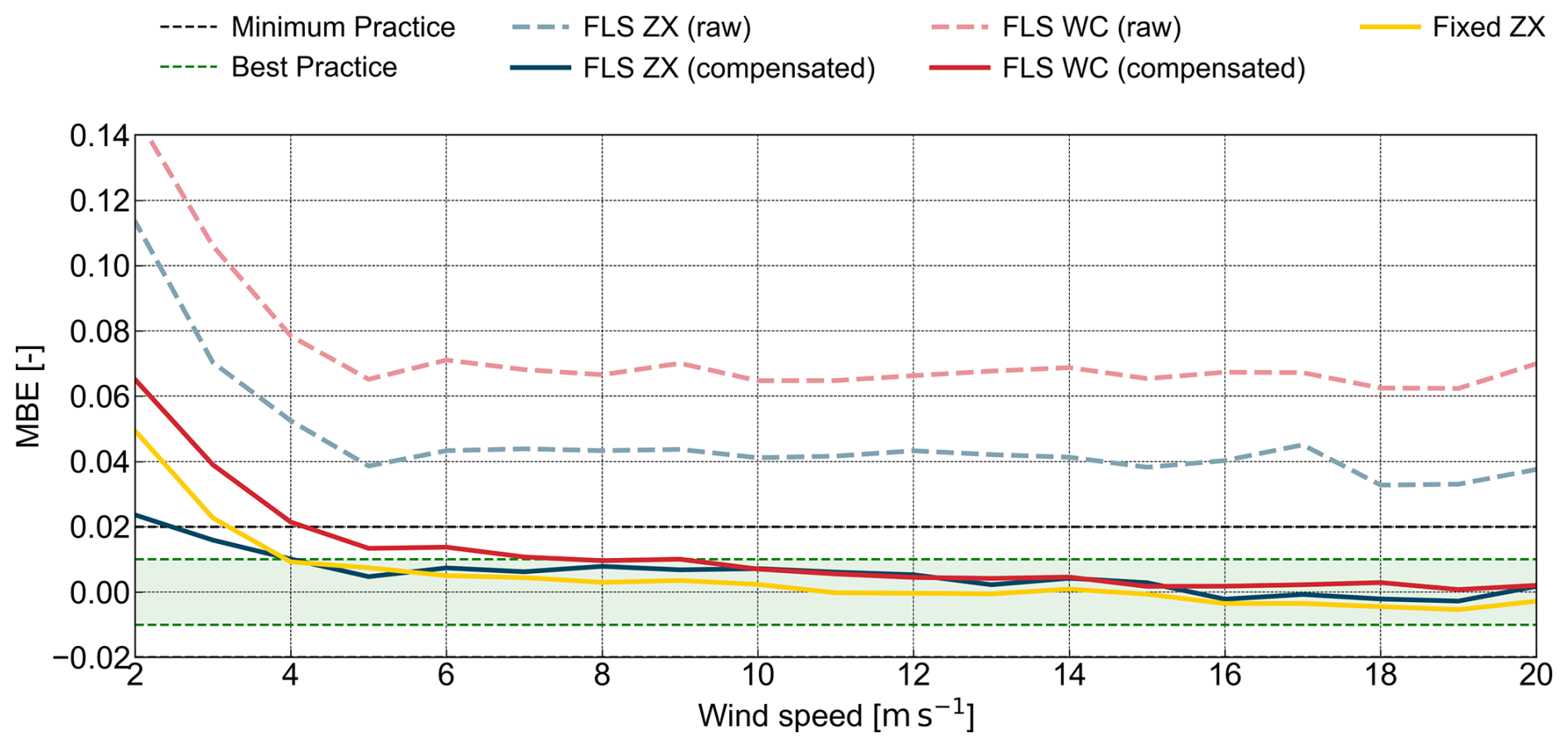
Figure 9 Binned mean bias error between the MM TI and the TI of the trialled device fixed ZX (yellow), FLS ZX (blue lines, where the dashed line represents raw data and the solid line depicts motion-compensated data), and FLS WC (red lines, where the dashed line represents raw data and the solid line depicts motion-compensated data) at 101 m above LAT.

The MBE trends in Fig. 9 demonstrate a clear distinction between the raw and motion-compensated datasets, illustrating the systematic overestimation of TI in the uncompensated data and the effectiveness of the compensation algorithm. Both raw datasets, represented by the dashed red and blue lines, consistently exhibit a positive bias across all wind speed bins. This bias is most pronounced at lower wind speeds below 5 m s⁻¹, where motion-induced fluctuations have a greater relative impact on TI due to the increased influence of platform movement in relation to wind speed. Moreover, TI values are generally higher at lower wind speeds, increasing the potential for greater bias in this range.

While both lidar types exhibit systematic TI overestimation in their raw datasets, the raw floating pulsed lidar TI (dashed red line) consistently shows a higher positive bias than the raw floating cw lidar TI (dashed blue line), while following a similar pattern until diverging for wind speeds higher than 17.5 m s⁻¹. This suggests that the pulsed lidar is more sensitive to motion-induced fluctuations, likely due to its sequential scanning method. In contrast, the cw lidar, which averages LoS velocities over a conical scan, appears to be less affected by motion variations, resulting in a lower overall bias in the raw data.

The fixed cw lidar also shows a relatively high bias at low wind speeds, which steadily declines until it approaches near-zero bias between 5 and 16 m s⁻¹. While this trend highlights the inherent differences between TI measurements from cw lidars and those derived from a cup anemometer, mast effects might also influence the measurements. Following motion compensation, the bias in both the floating pulsed (solid red line) and cw lidar (solid blue line) datasets is significantly reduced, confirming the effectiveness of the applied compensation algorithm. The floating pulsed lidar exhibits the most noticeable relative improvement, with a steep decline in bias at low wind speeds and a further reduction as wind speed increases. Despite this, the bias remains consistently positive across all wind speed bins, indicating that while compensation effectively mitigates motion effects, a small residual overestimation persists. For wind speeds between 4 and 9 m s⁻¹, the pulsed lidar falls well within the minimum practice range, before transitioning into the best-practice area for all higher wind speeds. The floating cw lidar maintains a low bias across all wind speed bins. Between 2.5 and 4 m s⁻¹, it remains below the 0.02 MBE line before entering the best-practice area. At 5 m s⁻¹, its error is slightly lower than that of the fixed cw lidar, before fluctuating within the best-practice range at higher wind speeds. Above 15.5 m s⁻¹, the MBE turns negative, following the same trend as the fixed cw lidar. While MBE provides insight into absolute bias, it does not fully capture relative errors, particularly at low wind speeds, where small absolute differences may result in large relative deviations. To address this, we examine the MRBE presented in Fig. 10.

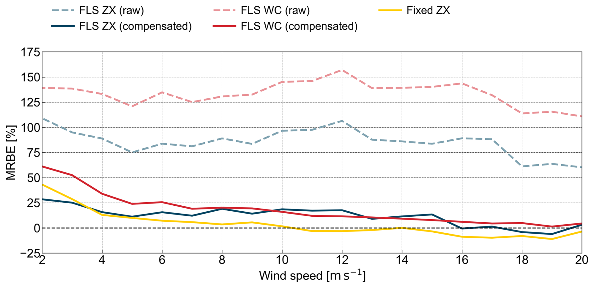
Figure 10 Mean relative bias error between the MM TI and the TI of the trialled device fixed ZX (yellow), FLS ZX (blue lines, where the dashed line represents raw data and the solid line depicts motion-compensated data), and FLS WC (red lines, where the dashed line represents raw data and the solid line depicts motion-compensated data) at 101 m above LAT.

The MRBE trends in Fig. 10 provide a complementary perspective to MBE. The raw datasets show extremely high MRBE values across all wind speeds, with the floating pulsed lidar reaching from about 125 % to 174 % and the floating cw lidar spanning from 60 % to 101 %. The fixed cw lidar MRBE remains stable across all wind speed bins, indicating that most of the bias is due to platform motion. Following motion compensation, the floating pulsed lidar again experiences the largest relative improvement, with an almost linear decline with increasing wind speeds. At higher wind speeds (between 10 and 15.5 m s⁻¹), the compensated pulsed lidar slightly outperforms the floating cw lidar while keeping a positive bias. This aligns with previous MBE findings that motion compensation is particularly effective for the pulsed floating lidar at higher wind speeds. For the floating cw lidar, the MRBE closely aligns with that of the fixed cw lidar at lower wind speeds before diverging around 5 m s⁻¹. While MBE is effectively reduced at wind speeds between 10 and 15 m s⁻¹, MRBE remains slightly elevated compared to the floating pulsed lidar.

3.3 Root mean square error and relative root mean square error

The RMSE trends in Fig. 11 illustrate the magnitude of absolute errors in TI measurements. The figure follows the same approach as Figs. 9 and 10, showing the error as a function of binned wind speed.

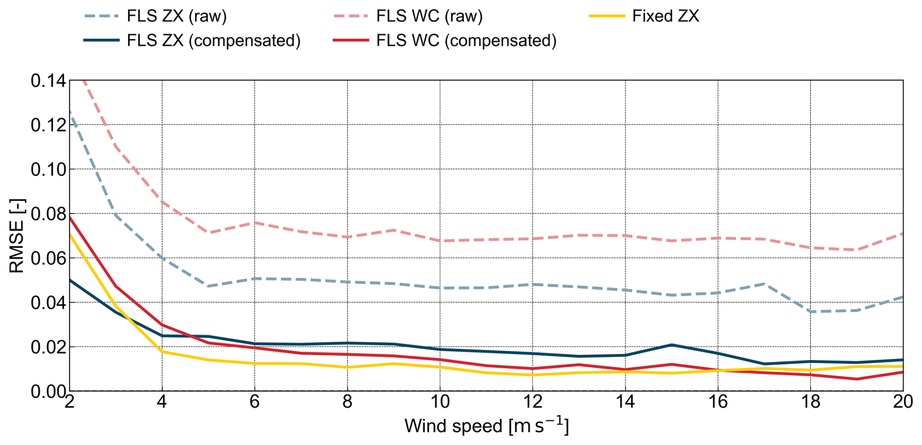
Figure 11 Binned root mean square error between the MM TI and the TI of the trialled device fixed ZX (yellow), FLS ZX (blue lines, where the dashed line represents raw data and the solid line depicts motion-compensated data), and FLS WC (red lines, where the dashed line represents raw data and the solid line depicts motion-compensated data) at 101 m above LAT.

Aligning with the trends from the MBE and MRBE analysis, the raw FLS datasets (dashed lines) exhibit substantially higher RMSE values compared to the fixed cw lidar. The highest RMSE values occur at lower wind speeds, gradually decreasing with increasing wind speed. While both lidar types exhibit high RMSE values in their raw datasets, the floating pulsed lidar (dashed red line) consistently shows greater RMSE than the floating cw lidar (dashed blue line). This suggests that, in addition to the higher systematic bias observed in MBE and MRBE, the motion introduces greater random errors into the pulsed lidar TI.

The fixed cw lidar (yellow line) exhibits a relatively high RMSE at low wind speeds, which steadily declines and stabilizes at a low level beyond 4 m s⁻¹. This trend again highlights the differences between TI measurements from cw lidars and those derived from a cup anemometer. Even without motion, RMSE does not reach zero, suggesting that part of the error arises from differences in measurement principles rather than motion alone.

Following motion compensation, RMSE is significantly reduced for both lidar types (solid blue and red lines).

The floating pulsed lidar TI (solid red line) experiences the largest relative improvement in RMSE, following a steep decline at low wind speeds. Notably, for wind speeds above 4.5 m s⁻¹, the RMSE in the pulsed lidar TI is lower than that of the floating cw lidar, and for wind speeds above 16 m s⁻¹, it even outperforms the fixed cw lidar, suggesting better alignment with the cup anemometer TI in high wind speed conditions. For the floating cw lidar, RMSE after motion compensation is clearly reduced but remains consistently higher than that of the floating pulsed lidar and fixed cw lidar across all wind speed bins beyond 3.5 m s⁻¹. This again indicates that while the compensation is effective, some residual motion effects may persist in the floating cw lidar TI measurements.

While RMSE provides a direct measure of absolute TI deviations, it does not account for how these errors scale with the TI magnitude itself. Since TI varies significantly across different wind speeds, an identical RMSE value at low and high wind speeds can have different implications for measurement accuracy. To capture this effect, we have analysed the RRMSE, presented in Fig. 12.

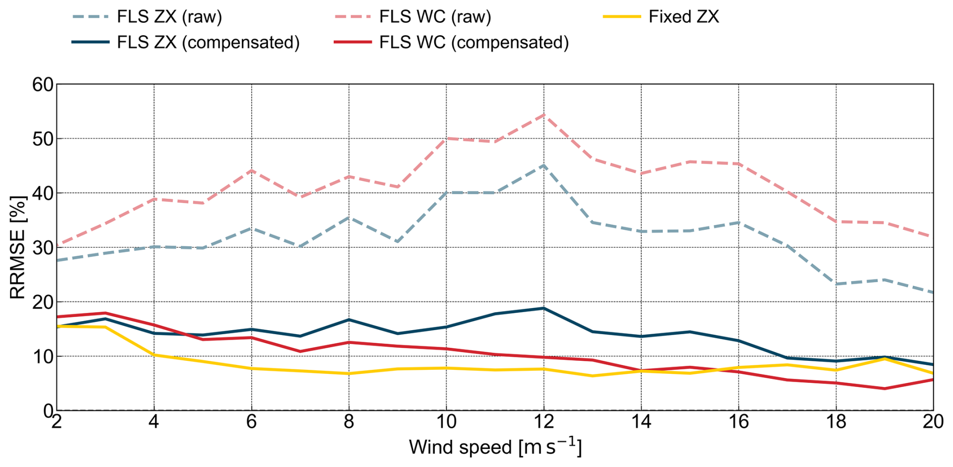
Figure 12 Relative root mean square error between the MM TI and the TI of the trialled device fixed ZX (yellow), FLS ZX (blue lines, where the dashed line represents raw data and the solid line depicts motion-compensated data), and FLS WC (red lines, where the dashed line represents raw data and the solid line depicts motion-compensated data) at 101 m above LAT.

The RRMSE trends in Fig. 12 reveal patterns that were less apparent in the RMSE results. While the RMSE decreases with increasing wind speed, the RRMSE remains relatively high across all wind speed bins, with peaks at moderate wind. Those peaks are particularly pronounced in the raw datasets (dashed lines).

The pulsed lidar (dashed red line) shows the highest RRMSE, reaching values of up to 56 %, while the floating cw lidar (dashed blue line) exhibits values between 30 % and 45 %. The fixed cw lidar TI RRMSE remains below 10 % across all wind speeds above 5 m s⁻¹, indicating the impact of the different measurement principles on the TI RRMSE. Following motion compensation, the floating pulsed lidar again exhibits the largest relative improvement, with RRMSE decreasing almost linearly as wind speeds increase. At wind speeds above 5 m s⁻¹, the compensated pulsed lidar performs better than the floating cw lidar. Above 14 m s⁻¹, the RRMSE of the floating pulsed lidar is even lower than that of the fixed cw lidar, indicating a better alignment of the pulsed lidars TI with cup anemometer TI. While the RMSE of the floating cw lidar decreases with increasing wind speed, the RRMSE fluctuates at lower wind speeds until reaching its peak around 19 % at the 12 m s⁻¹ bin. For wind speeds beyond 12 m s⁻¹, the RRSME decreases and almost aligns with the fixed cw lidar RRMSE around the 17 m s⁻¹ bin.

3.4 Representative TI error

While previous metrics provided valuable insights into bias and variability in the TI measurements, they do not necessarily indicate how well the lidar-derived TI represents statistical reference values for real-world applications (Q90). To assess the overall accuracy of TI estimates, we have analysed the representative TI error as a function of binned wind speed, as shown in Fig. 13, while utilizing the same approach as in the previous figures. Additionally, KPIs are indicated in Fig. 13, with the dashed black line representing the minimum practice threshold and the dashed green line denoting the best-practice range. The representative TI error was calculated according to Eq. (17) in Sect. 2.3.4, while using the Q90 values derived from the TI distributions.

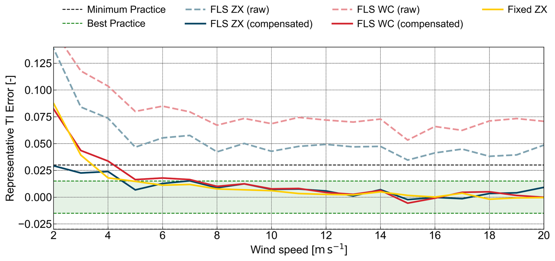
Figure 13 Representative TI error between the MM TI and the TI of the trialled device fixed ZX (yellow), FLS ZX (blue lines, where the dashed line represents raw data and the solid line depicts motion-compensated data), and FLS WC (red lines, where the dashed line represents raw data and the solid line depicts motion-compensated data) at 101 m above LAT.

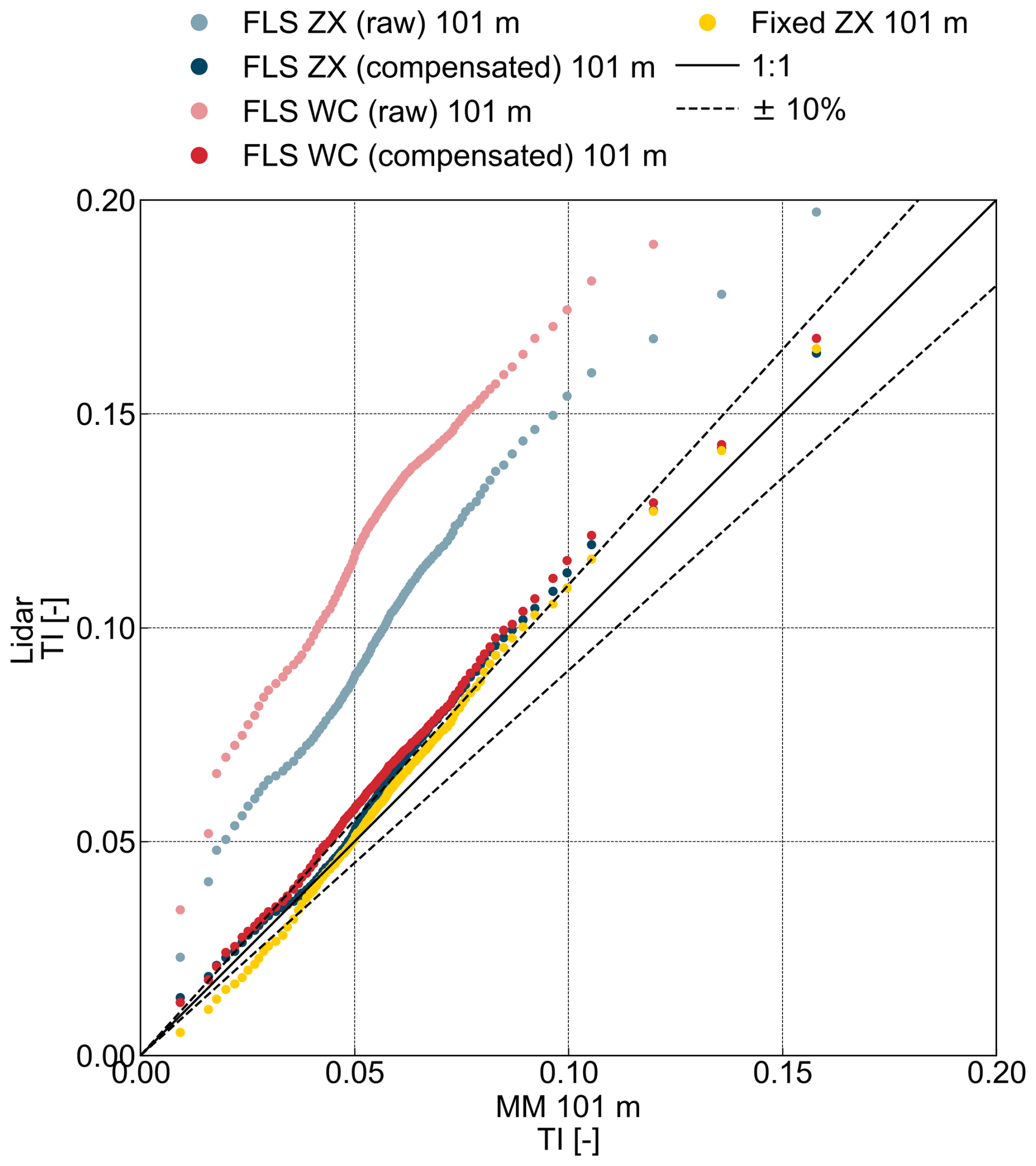
Figure 14 Quantile–quantile plot comparing the quantile distribution between the MM TI and the TI of the trialled device fixed ZX (yellow), FLS ZX (blue lines, where the dashed line represents raw data and the solid line depicts motion-compensated data), and FLS WC (red lines, where the dashed line represents raw data and the solid line depicts motion-compensated data) at 101 m above LAT.

Similar to previous metrics, the raw floating lidar datasets (dashed red and blue lines) exhibit substantially larger errors compared to its motion-compensated versions and the fixed cw lidar (solid lines).

The floating pulsed lidar (dashed red line) exhibits the highest representative TI error, followed by the raw floating cw lidar (dashed blue line). This is consistent with previous observations. The fixed cw lidar (yellow line) shows an initially high representative TI error which gradually decreases with increasing wind speeds. For wind speeds above 3 m s⁻¹, it reaches the minimum practice area before entering the best-practice range for wind speeds above 6 m s⁻¹. Beyond the 12 m s⁻¹ bin, the representative TI error almost aligns with the zero-error line. This suggests that cw lidar TI differs from cup anemometer TI at lower wind speeds. Following motion compensation, the representative TI error is significantly reduced for both lidar types. The floating pulsed lidar (solid red line) shows the greatest relative improvement. Following a steep decline in representative TI error at low wind speeds, it almost aligns with the fixed cw lidar trend for wind speeds beyond the 6 m s⁻¹ bin. For wind speeds above 14 m s⁻¹, the compensated pulsed lidar starts fluctuating around the zero-error line. The motion-compensated floating cw lidar trend (solid blue line) shows the lowest initial representative TI error, displaying an even lower error than the fixed cw lidar for wind speeds below 4 m s⁻¹. This is surprising and might be caused by mast wake effects or the smaller relative scan circle of the elevated fixed lidar. Overall, the representative TI error of the motion-compensated floating cw lidar decreases with increasing wind speed before passing the zero-error line at the 13 m s⁻¹ bin and fluctuating around it for wind speeds beyond that. However, at moderate wind speeds (9–15 m s⁻¹), the floating cw lidar retains slightly higher error values compared to the pulsed lidar.

3.5 Quantile-based distribution analysis

While previous analyses have focused on statistical errors and bias trends, a Q–Q plot provides an alternative way to evaluate how well the TI distributions align with the reference MM TI. Figure 14 presents a Q–Q plot comparing the floating (both raw and motion-compensated) and fixed lidar TI measurements against the MM TI at 101 m above LAT.

Viewed against the 1:1 and ±10 % guides, the behaviour of the FLS TI datasets (light blue and light red) is range dependent, while indicating systematic TI overestimation compared to met mast cup TI. The raw pulsed lidar (light red) exhibited the largest deviations, with deviations increasing as TI values rise. The raw cw lidar (light blue) displayed a lower offset. The small deviations shown by the fixed cw lidar (yellow) emphasize the difference between lidar and cup TI. Motion compensation significantly improves the agreement between floating lidar TI estimates and the MM reference. The motion-compensated datasets (blue and red dots) shift towards the 1:1 lines. The deviation from the ±10 % threshold is substantially reduced, confirming the effectiveness of the applied correction algorithm. The floating pulsed lidar (red dots) sees the most noticeable improvement, with compensated TI falling much closer to the 1:1 line. However, a slight overestimation persists, suggesting a minor systematic bias. The floating cw lidar (blue dots) also shows a strong improvement. For lower TI values, the distance to the 1:1 line is comparable to that of the fixed cw lidar, although its overestimating rather than underestimating.

At low TI (≲0.04), both compensated lines (blue/red) lie slightly above the 1:1 line, reflecting a small positive offset (residual overestimation) until they diverge near ≈0.04. The floating cw lidar then almost aligns with the fixed cw lidar, while the floating pulsed lidar trends marginally above the ±10 % band. At mid-range (≈0.05–0.08), the floating cw lidar diverges from the fixed cw lidar before clustering with the floating pulsed lidar slightly above the ±10 % band. Both raw lidar lines remain far outside that band, indicating how much motion-related deviation was removed by the compensation. At higher TI (≳0.08–0.11), the fixed cw lidar trends above the ±10 % band, almost converging with the compensated floating lidars. At very high TI (≈0.12–0.16), the compensated and fixed systems are well within the ±10 % band and close to the 1:1 line.

4 Discussion

While it is well established that deterministic motion compensation improves TI estimates from floating cw lidars, this study demonstrates for the first time that the same approach, when applied to pulsed systems operating at 5 Hz, yields TI bias convergence with floating cw lidars relative to a met mast reference under identical offshore conditions. A key outcome concerns the sampling timescale of pulsed systems. To our knowledge, this is the first published demonstration of a pulsed FLS operating offshore at 5 Hz effective sampling frequency with full deterministic compensation, showing that this configuration is sufficient in resolving turbulent timescales and delivering accurate TI estimates. In contrast, 1 Hz pulsed configurations (summarized in Appendix C) consistently overestimate TI even after deterministic motion compensation. This establishes sampling frequency as a decisive configuration parameter for pulsed lidars, with direct implications for their offshore use. Together, these findings demonstrate that, once motion effects are mostly mitigated, cw and 5 Hz pulsed systems provide comparable TI bias accuracy, with the pulsed lidar additionally showing a modest but consistent reduction in scatter-based metrics. With motion effects mostly mitigated, the reduction largely reflects lidar-specific behaviour.

To provide a comprehensive assessment in the absence of formal TI acceptance criteria, we report a multi-metric evaluation rather than relying on a single indicator. The discussion is structured into two main aspects: accuracy metrics, which assess systematic deviations (bias) between FLS and the reference measurement, and precision metrics, which evaluate the scatter and consistency of the measurements. In line with the study's framing, the discussion reflects on the three core factors identified as influencing FLS TI measurement performance: the lidar type, the platform-motion characteristics, and the motion-compensation method. In this experiment, the latter two were held constant – both lidars were deployed on FLSs of the same type under similar environmental conditions and were compensated using the same deterministic algorithm. This controlled configuration isolates the effect of lidar type, allowing for a direct assessment of how cw and pulsed systems respond to motion and compensation under otherwise similar conditions. Accuracy was primarily assessed through MBE, MRBE, and representative TI error. The raw FLS TI data exhibited a consistent positive MBE, meaning that both cw and pulsed lidars overestimated TI. This overestimation was stronger in the pulsed lidar data, likely due to sequential scanning and probe geometry interacting with short-term platform motions and turbulence. After motion compensation, the MBE was significantly reduced for both lidar types, particularly at moderate and higher wind speeds, indicating that motion-related contributions were largely addressed, and remaining bias differences are best attributed to lidar-specific behaviour. With deterministic compensation applied, the TI bias error of both systems relative to the cup reference converges, with frequent overlap and occasional cross-overs across wind speed bins, while residual differences remain minor. The MRBE results confirmed this trend, while revealing lower values for the pulsed lidar at moderate wind speeds. Overall, the analysis showed that the motion compensation effectively reduced relative bias across all wind speed bins. The compensated datasets showed near-zero bias at higher wind speeds, further validating the motion-compensation approach. The representative TI error analysis, which assesses the error in the 90th quantile of the TI distribution, a crucial parameter for wind turbine design applications, showed a notable improvement after motion compensation. The compensated datasets closely aligned with the suggested best-practice threshold, indicating that the motion-compensation algorithm successfully minimized systematic errors in TI estimates.

Precision was evaluated through RMSE, RRMSE, correlation analysis (R² and linear regression), and quantile-based distribution analysis. The RMSE results highlighted the impact of the motion compensation in reducing motion-induced scatter and improving measurement stability. The pulsed lidar initially exhibited the highest RMSE among the raw datasets, but after compensation, its RMSE was significantly reduced, surpassing the performance of the compensated cw lidar at higher wind speeds. The RRMSE, which normalizes RMSE, further confirmed this pattern. The motion-compensated pulsed lidar dataset showed the lowest RRMSE at high wind speeds, even outperforming the fixed cw lidar, indicating that a pulsed lidar TI aligns closer with a cup TI at higher wind speeds than a cw lidar TI.

Linear regression and correlation analysis demonstrated the overall improvement in agreement between FLS and reference data. The motion compensation notably increased the R² for both lidar types, with the pulsed lidar experiencing the largest relative improvement. We attribute the remaining scatter to three groups of effects: residual motion not corrected by the algorithm (e.g. small lidar–IMU timing offsets, heave/tilt-induced height variations), spatial configuration (e.g. instrument separation, elevation of the fixed cw lidar), and lidar-specific measurement-principle differences relative to the cup anemometers. The quantile-based distribution analysis (Q–Q plot) provided further insight into systematic over- and underestimation. The motion-compensated datasets exhibited better alignment with the reference data, reducing deviations across the distribution, with slight overestimation at low TI and a mild tilt towards underestimation at higher TI.

This study confirms that deterministic motion compensation significantly improves the accuracy and precision of FLS-derived TI measurements. While both lidar types benefitted from the algorithm, the pulsed lidar exhibited a greater relative reduction across all metrics and the lowest RMSE and RRMSE. The results from the representative TI error analysis further validate the efficiency of the FLS motion-compensation algorithm. The error of the resulting motion-compensated datasets closely aligns with that of the fixed cw lidar. As both lidars were mounted on FLSs of the same type (Fraunhofer IWES Wind Lidar Buoy) and only timestamps where all systems recorded data were considered, the observed differences are likely due to a combination of measurement-principle differences and lidar-specific coupling to platform motion. The systematic TI overestimation in the raw floating pulsed lidar data was consistently higher than that observed in the raw floating cw lidar measurements. This discrepancy is likely caused by the DBS scanning method of the pulsed lidar, where each LoS is measured sequentially at different azimuth angles, making it more sensitive to short-term platform motions. Although the deployed pulsed lidar was configured to collect data at an accelerated frequency of 5 Hz (compared to the 1 Hz standard configuration), the system was clearly more sensitive to motion than the cw lidar. A pulsed lidar of the same type with a lower scan frequency results in an even higher overestimation (see Appendix C). In contrast, the cw lidar performs continuous conical scans, averaging the measured LoS velocity and thereby already reducing the influence of rapid motions. The continuous scan with the 50 unsigned LoS measurements, however, appears to be more sensitive to small time offsets, which may lead to residual motion effects.

Direct numerical comparison across studies is limited, as available publications differ in their environmental envelopes and reporting practices. Sea state, wave conditions, and turbulence context are often not reported, and relative error metrics are rarely provided. Accordingly, the following comparisons focus on the magnitude and trend of reported absolute errors, while recognizing that differences in turbulence levels, compensation approach, and platform motions may explain part of the observed variation. Within these boundaries, our results are consistent in magnitude with those reported in prior studies applying a motion compensation to FLS.

In the study by Kelberlau et al. (2023), comparability is constrained by the fact that only absolute error metrics are reported. No information on sea state, turbulence information context (e.g. binned mean TI, Q90), or platform motion is provided. These boundaries should be kept in mind when relating their results to the present study. Kelberlau et al. (2023), who evaluate the performance of a deterministically motion-compensated cw lidar of the same type, report TI MBE within ±1 % and TI RMSE between approximately 0.14 % and 0.3 % for wind speeds between 4 and 16 m s⁻¹ at 101 m height (when considering bins with a representative number of data points). In the same study, the representative TI error of the motion-compensated FLS followed the trend of the fixed reference lidar and only diverged at wind speeds above 12 m s⁻¹, where sample sizes were limited. Overall, the error is well within ±1.5 % for wind speeds above 4 m s⁻¹. In our study, the MBE for the motion-compensated cw lidar similarly remained within ±1 %, while the compensated pulsed lidar slightly exceeded this range for wind speeds below 8 m s⁻¹. RMSE values for the cw lidar were marginally lower at low wind speeds, with both lidars showing nearly identical RMSE trends above 8 m s⁻¹. The pulsed lidar outperforms the cw lidar in both studies in terms of RMSE. The representative TI error for both motion-compensated lidar types in our study also closely followed the trend of the fixed reference lidar system, although with a slightly elevated error, particularly below 7 m s⁻¹. In terms of regression analysis, Kelberlau et al. (2023) compared binned motion-compensated cw lidar TI to both fixed cw lidar and mast references. While the OLS regression slope and intercept in our study closely match those reported, our Deming and RTO regression results were slightly closer to unity. Their R² values were marginally higher, likely due to the binning approach. Notably, the motion-compensated pulsed lidar in our study achieved the highest R², with values approaching 0.8.

In the case of Rapisardi et al. (2024), an ML-based compensation was applied. However, no descriptive statistics of the sea state, platform motion, or turbulence context are provided, which limits the ability to contextualize the reported error reductions. The evaluation does not include relative error metrics, restricting comparability to absolute measures. Rapisardi et al. (2024) applied ML-based motion-compensation models trained on either fixed lidar or anemometer data to cw (ZX Lidars ZX300M) FLS TI measurements. They evaluated the resulting compensated TI using OLS regression and MBE, referencing both fixed lidars and anemometers. Their results show a marked improvement in R² after compensation for both models, although slopes were not reported. However, their correlation plots show persistent underestimation in both raw and compensated TI, with the fixed-lidar-trained model slightly reducing this bias and the anemometer-based model increasing it. MBE was assessed at various heights and locations, both with training data from the same and from different met masts. In all cases, motion compensation reduced MBE to within the best-practice thresholds suggested by Kelberlau et al. (2023), consistent with the performance reported here. However, the raw (uncompensated) MBE in Rapisardi et al. (2024) was notably lower than in our study, likely reflecting differences in platform-motion characteristics and environmental conditions (sea-state information was not provided). Together, these results underscore that while individual metrics like MBE or R² can indicate performance improvements, they are insufficient on their own to comprehensively evaluate TI measurement accuracy. The observed underestimation in correlation plots despite favourable MBE values in Rapisardi et al. (2024) reinforces the importance of a multi-metric evaluation approach. These comparisons highlight the fact that TI measurement accuracy from FLS is governed by a combination of factors: the deployed lidar type, the dynamic response of the floating platform, and the applied motion-compensation method.

In Uchiyama et al. (2024), environmental conditions are well characterized, with statistics reported for sea state, wave parameters, and TI distributions, providing valuable context for interpreting the results. The study evaluated the binned 90th percentile of TI (Q90) for three different FLS types (buoy, ship, and spar buoy) against reference measurements from a fixed Vaisala WindCube V2.1 and cup anemometers but did not apply motion compensation. The buoy-based system was equipped with a ZX Lidars ZX300M, the ship-based system with both a ZX Lidars ZX300M and a Vaisala WindCube, and the spar buoy with a Mitsubishi Electric Diabrezza (pulsed lidar). The cw lidar on the buoy-type FLS showed significant overestimation, while the same lidar on the ship-type system yielded Q90 values much closer to the fixed references. Compared to the uncompensated cw lidar in our study, the overestimation observed in the buoy-type system appears relatively high. The ship-based FLS showed lower Q90 errors for both lidar types, with the pulsed lidar displaying the larger deviation, which is consistent with our findings. The spar-buoy system showed good agreement with the reference, suggesting a lower influence of motion. It should also be noted that the reference curves differ between the plots, indicating that different time periods may have been used for each comparison. This limits the ability to directly compare lidar performance across FLS types. In contrast, our study uses a controlled setup with platforms of the same type, co-located deployments, and a shared motion-compensation method. This allows us to systematically isolate the effects of platform motion, lidar type, and compensation approach, thereby expanding on the insights provided by Uchiyama et al. (2024).

Despite the successful demonstration, the findings of this study are explicitly bounded to the 3-month North Sea calibration campaign (which lacks seasonal variability), the buoy type deployed, and the associated environmental envelope (see Sect. 2.4). In the present campaign, synchronization and motion sensing were sufficient in meeting the requirements for deterministic motion compensation during extreme sea states (mentioned in the Introduction), as residual errors showed no systematic dependence on significant wave height or peak period across the observed envelope. Broader generalization will require additional deployments across wider ranges of environmental conditions and FLS types. The comparison presented here was restricted to specific commercial implementations of cw and pulsed systems against a cup anemometer reference (industry standard). Other reference devices or lidar device configurations, such as alternative probe lengths, beam geometries, or pulsed sampling rates, were not tested and could influence quantitative outcomes. Moreover, atmospheric stability stratification was not performed, leaving stability-dependent behaviour as an important factor for future investigation. The fixed cw lidar on the mast was treated only as a plausibility check that deterministic compensation removed the platform–motion imprint, not as an accuracy reference. The potential limitation of cw homodyne detection in combination with a deterministic motion-compensation approach did not manifest in the data. However, it could be a factor contributing to the elevated error in scatter-based metrics. Because platform and mast positions were fixed, we cannot isolate spatial separation effects in this dataset. We acknowledge any contribution but leave it unquantified.

The practical implication of these results is that deterministic motion compensation provides a transparent and effective baseline for floating lidar turbulence measurements. Within the tested environmental envelope, it removes motion-induced bias to industry-relevant levels for both cw and (5 Hz) pulsed systems. While the pulsed lidar consistently exhibited a modest advantage in scatter-based metrics, dispersion remains the main limitation. This difference, although small, may be relevant for applications that are more sensitive to dispersion than to mean bias. Importantly, this trial empirically establishes that for pulsed deployments, a 5 Hz effective scan frequency is necessary and sufficient to achieve comparability with fixed-system references, whereas a 1 Hz configuration undersamples turbulence and motion timescales and cannot resolve them reliably. At the same time, the absence of a decisive advantage of the 50 Hz cw system over the 5 Hz pulsed case shows that ever-higher effective sampling rates are not inherently beneficial for 10 min TI estimation. Instead, the decisive factor is matching sampling resolution to the dominant timescales of platform motion and turbulent fluctuations, which the 5 Hz configuration adequately resolves.

Taken together, the results underline the importance of a multi-metric evaluation approach to capture both systematic bias and variability. They further show that deterministic motion compensation enables both lidar types to meet offshore operational requirements, while providing actionable guidance: adopt deterministic compensation as a baseline, configure pulsed systems at 5 Hz, and recognize that cw-pulsed differences after compensation are secondary and use-case dependent.

Future work should extend these findings beyond the present campaign by expanding testing across different buoy types and sea-state conditions. The present trial used a buoy-type platform that reacts to the sea state in a relatively slow and inert manner, with predominantly periodic swinging and heaving that are well suited to deterministic compensation. Ship-type systems that follow the wave crests more directly are expected to exhibit shorter-period less periodic motions, which may prove more difficult to correct. Deterministic compensation itself could be further refined through improved time synchronization between motion sensors and lidar sampling. Another important direction is the systematic comparison of different motion-compensation types under identical sea-state and platform-response conditions. Sensitivity analyses are required to evaluate how deterministic compensation responds to varying motion characteristics and environmental variables such as atmospheric stability. In parallel, the role of lidar-specific parameters, including probe length, beam geometry, and internal processing choices (held constant in this trial), as well as carrier-to-noise ratio (CNR) and data availability, should be systematically isolated. Further, while deterministic compensation should remain the transparent foundation for industry applications, ML post-processing may be explored as a secondary layer to further reduce scatter. Such approaches must be applied with caution as they introduce black-box behaviour and should be constrained to lidar-specific sensitivities, not site-specific effects (e.g. wakes or other external influences).

5 Conclusions

This study evaluated the accuracy and precision of FLS TI measurements by comparing raw and motion-compensated TI data from two different lidar types – cw and 5 Hz pulsed – as well as fixed cw lidar TI data, against a met mast cup anemometer reference. Both floating lidars were mounted on FLS platforms of the same type, operated under identical offshore conditions, and corrected using the same deterministic motion-compensation algorithm. This setup allowed the effect of lidar type on TI measurement performance to be isolated under controlled conditions. The results demonstrate that motion-induced overestimation in raw pulsed and cw FLS TI data can be effectively mitigated through deterministic motion compensation, significantly reducing both systematic bias and scatter.

After compensation, TI bias of both lidar types converged towards the cup reference, with residual bias near zero across most wind speed bins and only small bin-to-bin differences that do not support a systematic ranking between the principles, while the pulsed system showed a modest advantage in scatter-based metrics. Importantly, this trial represents, to our knowledge, the first reported offshore deployment of a pulsed FLS operating at 5 Hz with full deterministic compensation. While Appendix C shows that 1 Hz is insufficient in resolving the relevant turbulence timescales, the present results provide empirical evidence that 5 Hz is sufficient and achieves industry-relevant TI accuracy after deterministic compensation. The lack of a decisive advantage of the 50 Hz cw system over the 5 Hz pulsed case indicates that ever-higher sampling rates are not inherently beneficial for 10 min TI.

These findings confirm that properly motion-compensated cw and 5 hz pulsed FLS can provide TI measurements comparable to fixed-system references for offshore site assessment. Practically, these contributions offer actionable guidance for the offshore wind sector: adopt deterministic motion compensation as a transparent baseline, configure pulsed systems at 5 Hz, and use the presented multi-metric evidence base to support acceptance decisions in the absence of prescriptive standards.

Future work should focus on refining deterministic compensation to reduce the residual dispersion by improving sensor synchronization and accounting for lidar-specific sensitivities, while validating performance across different platforms, sea states, and environmental conditions. Another important direction is the systematic comparison of different motion-compensation types under identical sea-state and platform-response conditions. Sensitivity studies should also be conducted to assess the influence of motion characteristics, atmospheric stability, and lidar configuration parameters. Machine learning post-processing may provide additional benefit as a secondary layer, provided it is applied cautiously and transparently.

Appendix A: Lidar retrieval methods

The ZX Lidars ZX300M cw wind lidar used in this study employs the VAD technique to retrieve horizontal wind speed and direction. This method assumes horizontal homogeneity of the wind field and estimates wind components based on Doppler shift measurements taken at multiple azimuth angles during a conical scan. Following Browning and Wexler (1968), for azimuth θ and half-cone opening angle α,

$$\begin{array}{}\text{(A1)}& v_r\left(\mathit{\theta }\right)=a_{\mathrm{0}}+a_{\mathrm{1}}\cos \mathit{\theta }+b_{\mathrm{1}}\sin \mathit{\theta },\end{array}$$

where a₀, a₁, and b₁ are estimated by least squares over each scan. The fitted coefficients correspond to the wind vector components

$$\begin{array}{}\text{(A2)}& v_x={\displaystyle \frac{b_{\mathrm{1}}}{\sin \mathit{\alpha }}},v_y={\displaystyle \frac{a_{\mathrm{1}}}{\sin \mathit{\alpha }}},v_z={\displaystyle \frac{a_{\mathrm{0}}}{\cos \mathit{\alpha }}}.\end{array}$$

The deployed ZX300M model uses homodyne detection and therefore reports unsigned radial velocities. To sign the radial velocities before solving and to resolve the 180° ambiguity, a reference wind direction from a collocated weather station is used by the ZX300M units.

The Vaisala WindCube pulsed wind lidars use the DBS method, which involves sequentially directing the laser beam along five fixed angles to reconstruct the three-dimensional wind vector. Like VAD, DBS also assumes horizontal homogeneity and relies on the trigonometric reconstruction of wind components from the measured radial velocities. Following Pauscher et al. (2016), the DBS model for beam i with azimuth α_i is

$$\begin{array}{}\text{(A3)}& v_{r,i}=(u\cos {\mathit{\alpha }}_i+v\sin {\mathit{\alpha }}_i)\sin \mathit{\varphi }+w\cos \mathit{\varphi }.\end{array}$$

The wind vector components are retrieved per scan by least squares over all available beams. The Vaisala WindCube V2.1 deployed in this study uses simplified pair-difference equations instead of a least-squares inversion:

$$\begin{array}{}\text{(A4)}& u={\displaystyle \frac{v_{r,\mathrm{0}}-v_{r,\mathrm{180}}}{\mathrm{2}\sin \mathit{\varphi }}},v={\displaystyle \frac{v_{r,\mathrm{90}}-v_{r,\mathrm{270}}}{\mathrm{2}\sin \mathit{\varphi }}},w=v_{r,\text{vert}}.\end{array}$$

Both lidars reconstruct the wind vector under horizontal homogeneity using numerical fitting. Vendor-specific filtering and implementation details are proprietary.

Appendix B: Mean horizontal wind speed correlation plot

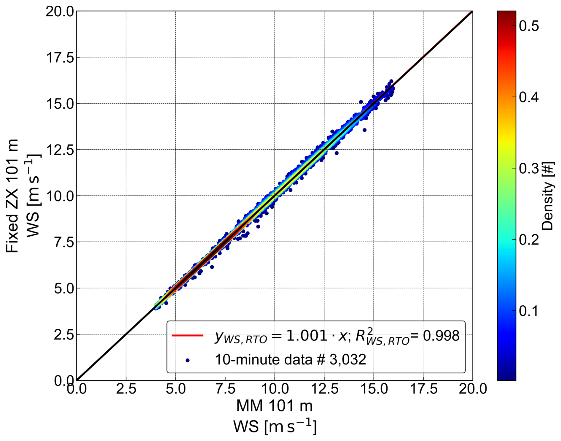
Figure B1 Density correlation plots and regression analyses of horizontal mean wind speed measured by the fixed cw lidar (fixed ZX) versus the FINO3 met mast cup (MM) at 101 m above LAT. Point density is indicated by the colour bar.

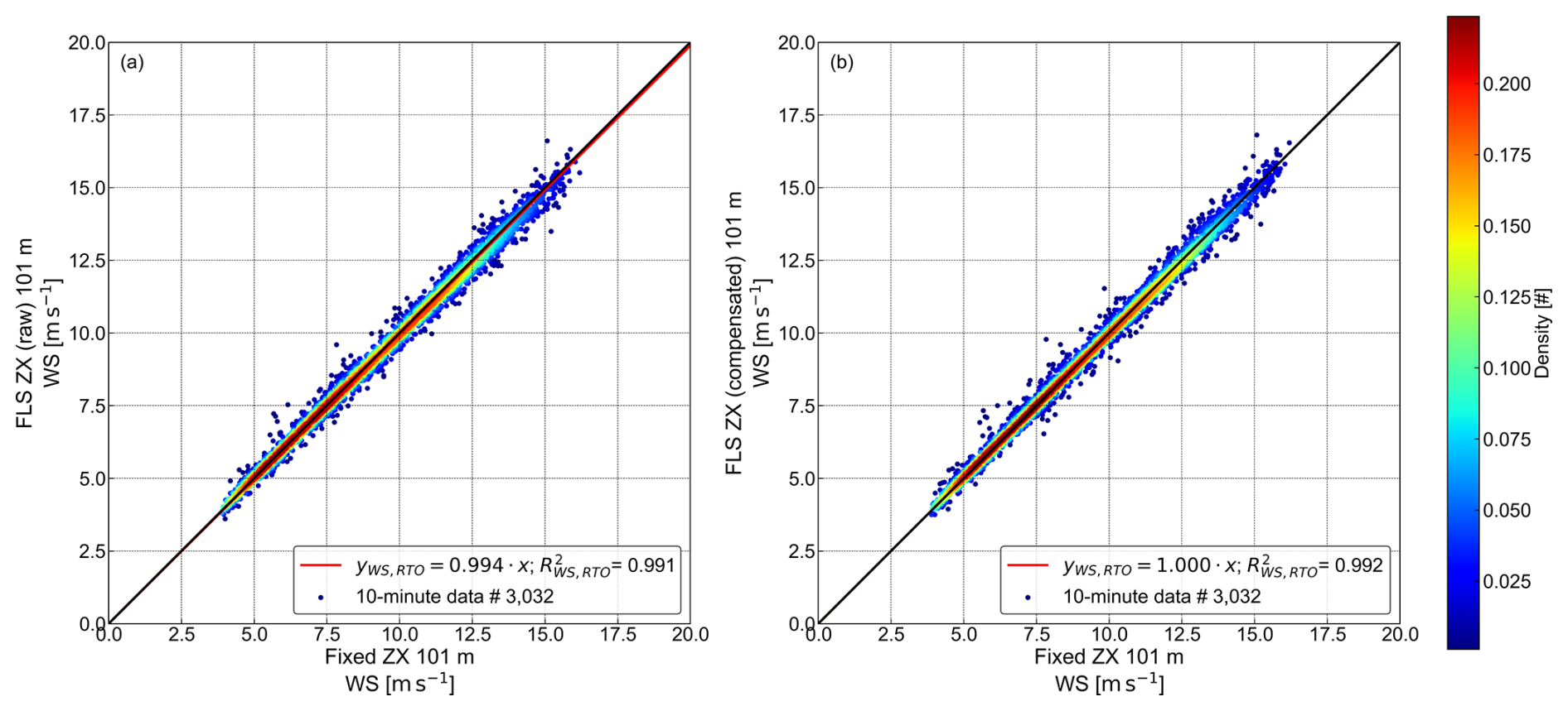
Figure B2 Density correlation plot and regression analysis of horizontal mean wind speed measured by the floating cw lidar (FLS ZX) versus the fixed cw lidar (fixed ZX) at 101 m above LAT. Panel (a) shows uncompensated (raw) data, while panel (b) shows motion-compensated data. Point density in both panels is indicated by the colour bar.

Figure B3 Density correlation plots and regression analyses of horizontal mean wind speed measured by the floating cw lidar (FLS ZX) versus the FINO3 met mast cup (MM) at 101 m above LAT. Panel (a) shows uncompensated (raw) data, while panel (b) shows motion-compensated data. Point density in both panels is indicated by the colour bar.

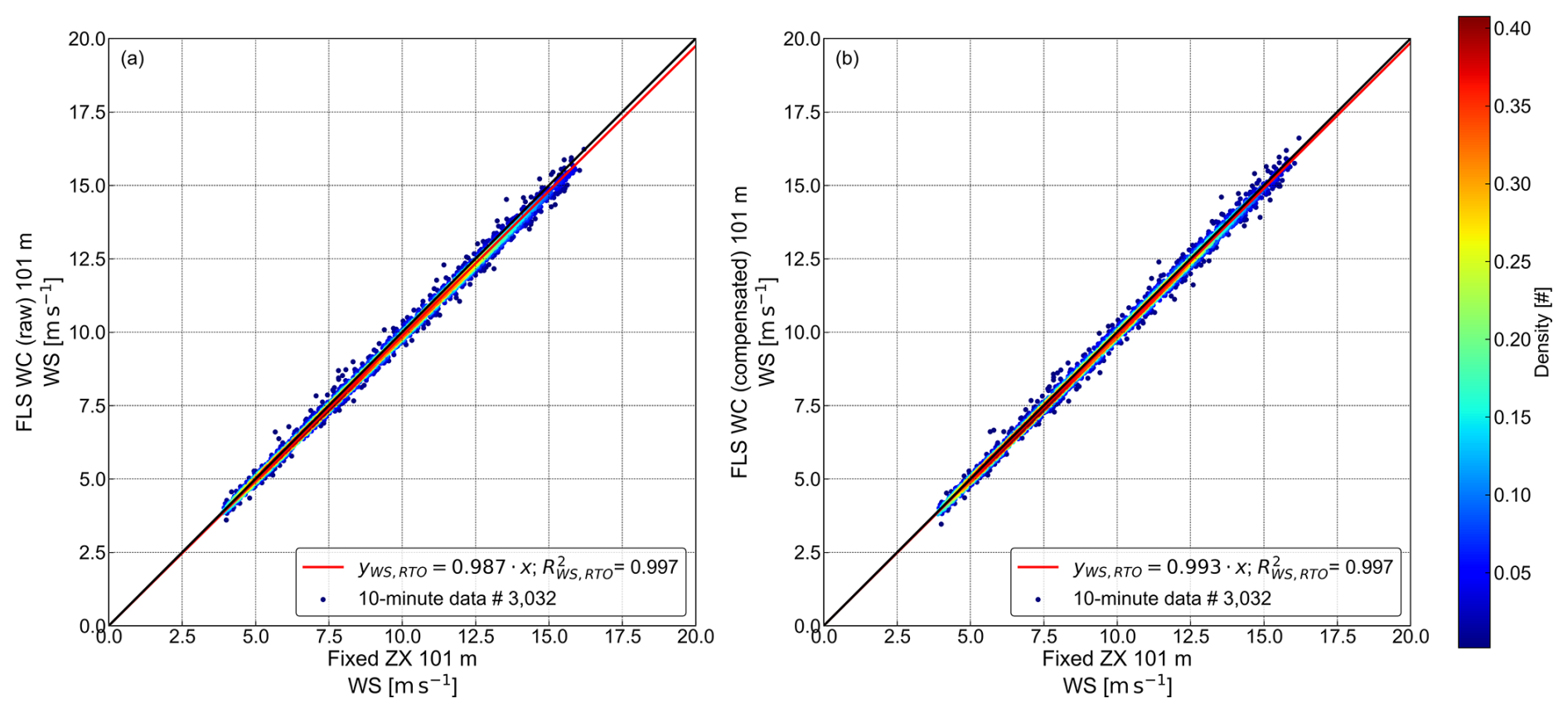
Figure B4 Density correlation plots and regression analyses of horizontal mean wind speed measured by the floating pulsed lidar (FLS WC) versus the fixed cw lidar (fixed ZX) at 101 m above LAT. Panel (a) shows uncompensated (raw) data, while panel (b) shows motion-compensated data. Point density in both panels is indicated by the colour bar.

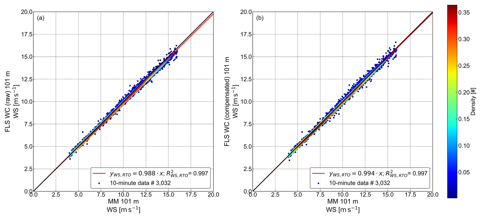
Figure B5 Density correlation plots and regression analyses of horizontal mean wind speed measured by the floating pulsed lidar (FLS WC) versus the FINO3 met mast cup (MM) at 101 m above LAT. Panel (a) shows uncompensated (raw) data, while panel (b) shows motion-compensated data. Point density in both panels is indicated by the colour bar.

Appendix C: Pulsed lidar at 1 Hz effective sampling frequency

The results presented in this appendix show FLS TI data from a FINO3 calibration trial of a Fraunhofer IWES Wind Lidar Buoy equipped with a Vaisala WindCube V2.1 pulsed lidar in the commercial standard 1 Hz effective sampling frequency configuration (FLS WC 1 Hz). The data cover the period from 6 September 2021, 00:00:00 to 3 November 2021, 00:00:00 UTC, during which a wide spectrum of sea-state and wind conditions were covered, which is presented in Fig. C1.

The deterministic motion-compensation algorithm was applied to the FLS WC 1 Hz dataset. To assess the effect of this compensation, the FLS WC 1 Hz TI (blue lines) is compared with TI from the FINO3 met mast cup anemometer at 101 m above LAT, using the performance metrics introduced in Sect. 2.3 (see Fig. C2). In addition, to enable a qualitative comparison of motion compensation between the 1 and 5 Hz effective sampling frequency configurations of floating pulsed lidars, results from the present campaign (Sect. 2.4) are also included (red lines).

It must be noted, however, that the datasets were obtained during different deployments at FINO3. Consequently, the environmental conditions, particularly the prevailing sea state, were not identical across campaigns. We therefore stress that this comparative overview is strictly indicative.

The trends in Fig. C2 highlight the pronounced TI overestimation of the FLS operated at a 1 Hz effective sampling frequency across all panels. In panel (a), the binned mean TI shows that the raw FLS WC 1 Hz systematically overestimates TI by a factor of ≈2–4 compared to the cup anemometer reference. Moreover, this overestimation increases with wind speed, suggesting a strong influence of platform motion on the derived TI. In contrast, the 5 Hz configuration exhibits a lower overestimation (around a factor of ≈2 %) and shows no clear dependence on wind speed.

The error metrics in panels (b) and (c) support these observations, with RMBE reaching up to ≈360 % and RRMSE up to ≈75 % for the 1 Hz configuration. Motion compensation proves highly effective in reducing this bias, with a particularly strong impact on the 1 Hz data. However, even after compensation, the MBE/RMBE and RMSE/RRMSE of the 1 Hz data remain elevated compared to the compensated 5 Hz configuration.

The wind speed dependence of the 1 Hz overestimation can be explained by the interaction of platform motion with the lidar measurements. As wind speed rises, motion-induced fluctuations project more strongly into the wind retrieval, amplifying the TI. At the same time, because true TI is typically low at high wind speeds, the absolute error translates into a much larger relative overestimation at higher wind speeds. The sampling rate of 1 Hz further amplifies this issue, as it cannot sufficiently resolve the dominant frequencies of platform motion, leading to aliasing effects and inflated TI estimates.

Interestingly, the representative TI error (Q90 error, panel d) of the 1 Hz configuration remains small at high wind speeds and meets best-practice criteria above 11.5 m s⁻¹. This is consistent with the generally lower TI at high wind speeds, which reduces the relative impact of motion-induced fluctuations.

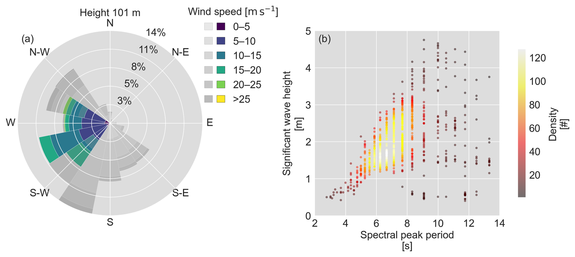
Figure C1 Statistical overview of reference conditions recorded during the 1 Hz WindCube trial: (a) wind rose displaying wind direction distribution measured by the wind vane at 101 m LAT along with the corresponding bin-wise wind speed distribution from the cup anemometer at the same height (grey scales correspond to the whole campaign period, while blue/green scales represent the selected timestamps); (b) significant wave height versus spectral peak period density correlation plot measured by the waverider buoy in proximity to the met mast.

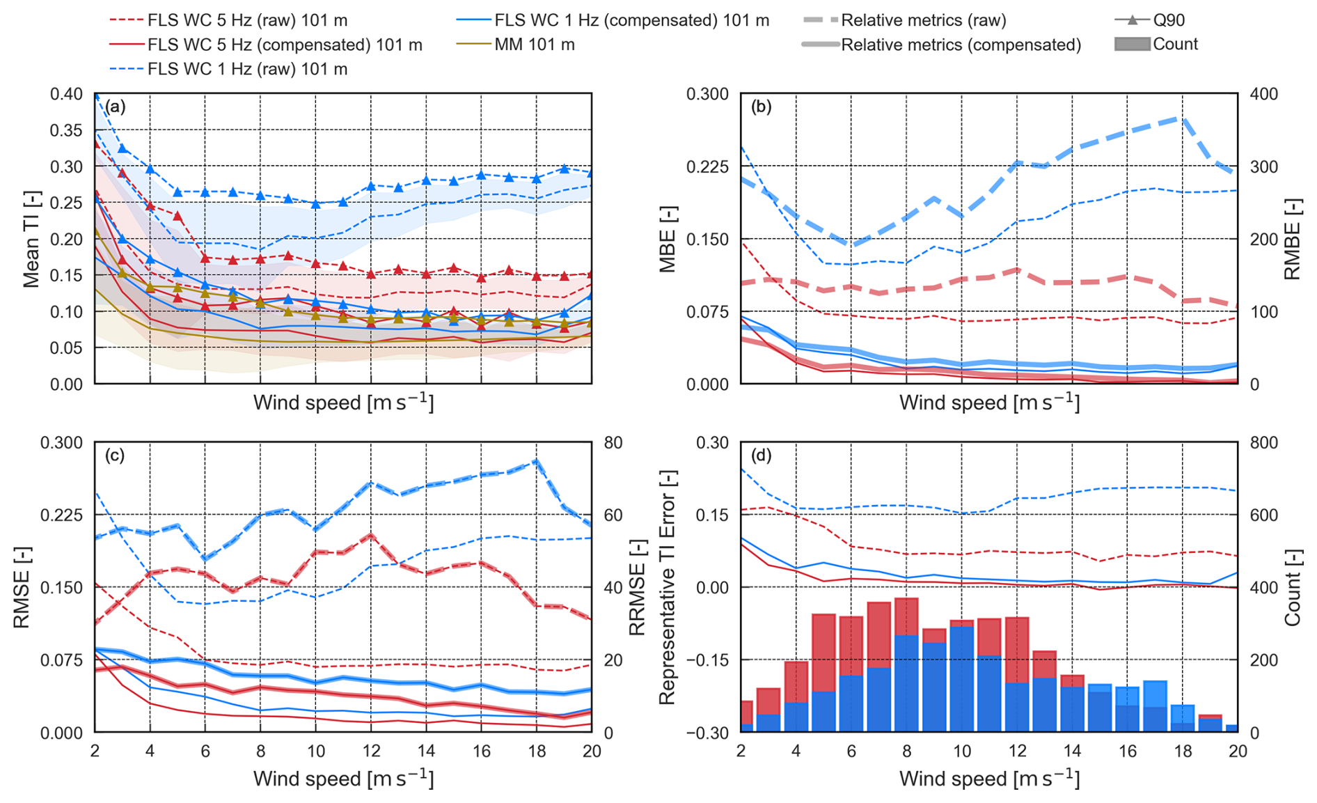
Figure C2 TI error between the MM TI and the TI measured by the device FLS WC 5 Hz (red) and FLS WC 1 Hz (blue) from a separate campaign, at 101 m above LAT. Dashed lines indicate raw data, while solid lines indicate motion-compensated data. Panels show (a) mean TI, standard deviation, and Q90; (b) TI MBE and RMBE; (c) TI RMSE and RRMSE; and (d) representative TI error as well as count.