Experimental study of regenerative wind farms featuring enhanced vertical energy entrainment

This study presents the experimental validation of regenerative wind farms (RGWFs), a novel wind farm concept designed to enhance overall wind farm performance. RGWFs employ multi-rotor systems with lifting devices (MRSLs), an innovative wind energy harvester engineered to stimulate strong vertical energy entrainment, thereby accelerating wake recovery. In the experiments, MRSLs are scaled for wind tunnel testing, with their rotors modeled using porous disks and their lifting devices represented by wings. The tested RGWFs comprise up to 3×3 MRSLs. Flow quantities within RGWFs and aerodynamic loads on MRSLs are measured using volumetric particle tracking velocimetry and strain gauges. Compared to conventional wind farms, flow analysis indicates that vertical energy entrainment is significantly enhanced in RGWFs, as evidenced by a more than 200 % increase in thrust on the second-row MRSLs and so on. These experimental results, which are in line with the previous numerical predictions, highlight the promising potential of RGWFs.

1 Introduction

In recent decades, offshore wind energy has demonstrated its economic viability as a renewable energy source (Williams and Zhao, 2024). The profitability of offshore wind farms has largely been driven by cost reductions achieved through the close spatial arrangement of turbines and the continual increase in turbine size (Sørensen and Larsen, 2021). However, the levelized cost of energy (LCoE) for offshore wind remains relatively high compared to other technologies, such as gas combined cycle and solar photovoltaic system (Lazard, 2024). Furthermore, since the most economically favorable sites have already been developed and the relative costs of curtailment and energy storage systems are rising with the increasing total capacity (Wind Europe, 2024; Lazard, 2024), the LCoE of offshore wind could increase further in the foreseeable future. These factors render offshore wind more susceptible to macroeconomic challenges (McCoy et al., 2024). For instance, several high-profile offshore wind projects in North America and Europe have been delayed or (partly) canceled due to escalating interest rates (Empire Wind, 2025; Ørested, 2025; McCoy et al., 2024). In light of these challenges, the current offshore wind market urgently calls for engineering solutions to reduce the LCoE and enhance the industry's competitive position.

One of the primary physical limitations preventing further reductions in the LCoE of offshore wind is the losses caused by turbine–turbine wake interactions within wind farms, which reduce the overall farm efficiency by 10 % to 25 % (Barthelmie et al., 2009, 2010). Consequently, mitigating wake losses holds significant potential for improving wind farm performance and, in turn, lowering the LCoE of offshore wind. To address this issue, Ferreira et al. (2024) recently proposed a novel wind-energy-harvesting machine, which is the multi-rotor system with lifting devices (MRSL). An MRSL comprises an array of wind turbine rotors mounted on a scaffolding structure, as depicted in Fig. 1. In addition, it incorporates large stationary wing elements that generate strong tip vortices. These vortices are intended to enhance mixing between the wake and the ambient flow in the vertical direction, thereby accelerating the wake recovery process. Conceptually, the lifting devices operate similarly to the vortex generators used on aircraft wings, albeit on a much larger scale (Ferreira et al., 2024). Notably, as mentioned by Li et al. (2025c), it is the lifting device being the essential component to enhance the wake recovery rate, regardless of the specific implementation approach – that is, whether the energy-harvesting element is a conventional single-rotor horizontal-axis wind turbine or a system with multiple vertical-axis wind turbines, the principle remains effective as long as large-scale lift-generating elements are incorporated. Among the possible implementations the authors have thought of, the MRSL configuration shown in Fig. 1 is considered to be the most practical realization of this concept by the authors, as the scaffolding structure readily accommodates the integration of the lifting devices.

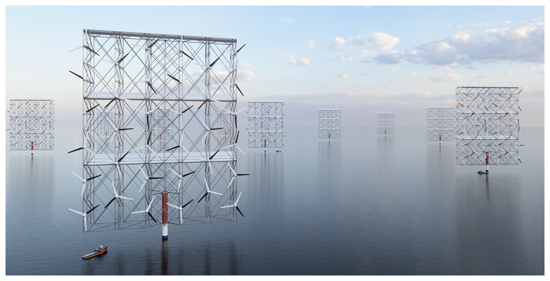
Figure 1 Computer-rendered visualization envisioning the multi-rotor system with lifting devices (MRSL) and a regenerative wind farm (RGFW) deployed in offshore locations. With the authors' current idea, the MRSL is envisioned to be approximately 300 m in both width and height, with a clearance of 30 m above the sea surface. Image courtesy of Carraro et al. (2024).

Recent studies have shown, both experimentally and numerically, that the lifting devices of an isolated MRSL can significantly accelerate its wake recovery. In particular, Broertjes et al. (2024) tested a scaled MRSL in an open-jet wind tunnel. The tested configuration consisted of an array of 16 vertical-axis wind turbines and two wings, with overall dimensions of 1.43 m in width and 1.35 m in height. Their results indicated that the MRSL's wake is effectively deflected vertically due to the influence of the lifting devices. However, due to the spatial limitations of the wind tunnel, their analysis is restricted to the near-wake region ($x/D>\mathrm{2}$, where x is the streamwise distance and D is the width of the tested MRSL). On the numerical side, the studies of Avila Correia Martins et al. (2025) and Li et al. (2025b) employ computational fluid dynamics (CFD) solvers with actuator-based methods. Their results show good agreement with the experimental findings of Broertjes et al. (2024) in the near-wake region and provide evidence that the lifting devices are able to significantly enhance vertical mixing and accelerate wake re-energization in the far wake ($\mathrm{3}<x/D<\mathrm{8}$). Regarding the wind farms composed of MRSLs, which are termed regenerative wind farms (RGWFs) by Ferreira et al. (2024), a recent numerical study by Li et al. (2025c) using CFD with RANS (Reynolds-averaged Navier–Stokes) approach showed that wake-induced power losses within RGWFs are reduced to approximately one-third of those observed in wind farms using a multi-rotor system without lifting devices. In simpler words, the studied RGWFs achieved roughly twice the efficiency of their conventional counterparts.

To further evaluate the practical viability of RGWFs, this study conducts comprehensive wind tunnel experiments with scaled wind farms having an array of 3×3 or 3×2 MRSLs. In these experiments, MRSLs are aerodynamically represented by porous disks with wings attached. Three MRSL configurations are tested. The first is designed to eject the wake upward (Up-Washing), the second is configured to direct the wake downward (Down-Washing), and the last is a reference configuration that is without the lifting devices (Without-Lifting) for benchmarking. Both the aerodynamic loads on MRSLs and the surrounding flow fields are measured. The flow fields are captured using three-dimensional particle tracking velocimetry (3D-PTV). Furthermore, wind farm layouts with MRSLs aligned and staggered with respect to the inflow direction are both examined.

2 Methodology

2.1 Wind tunnel and general experimental setup

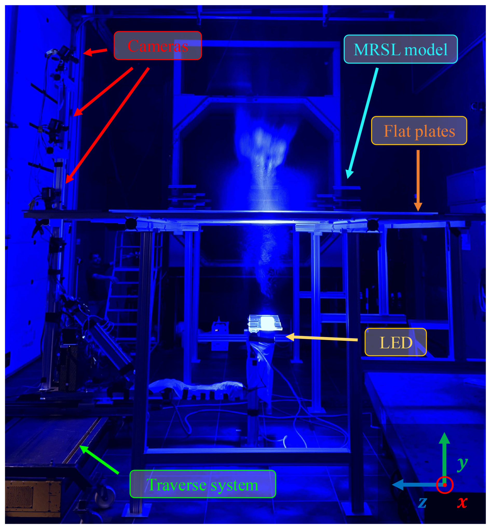
The scaled RGWFs are experimentally tested in the Open Jet Facility (OJF) at the aerodynamic laboratories of Delft University of Technology (TU Delft). OJF is an atmospheric closed-circuit open-jet wind tunnel, and it features an octagonal outlet measuring 2.85×2.85 m² (see Fig. 2). Additional specifications of OJF are provided in Lignarolo et al. (2014).

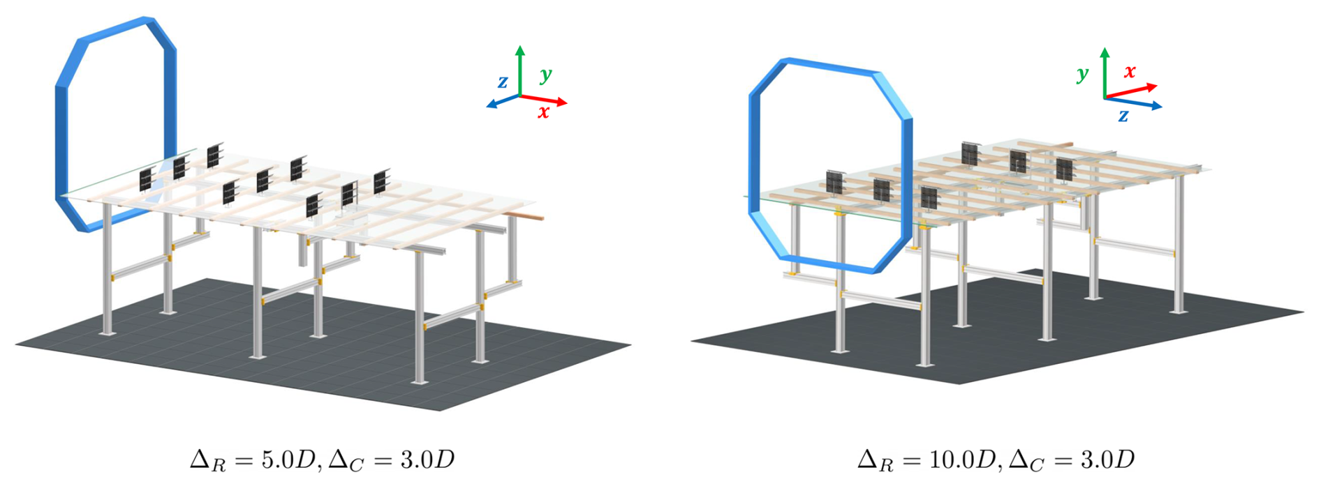
Figure 2 Illustration of the experimental setups for the regenerative wind farms with the aligned layout. Δ_R and Δ_C are the row (x direction) and the column (z direction) spacings, respectively. The left panel shows a wind farm with Δ_R=5.0D and MRSLs in the Up-Washing configuration (UW-05). The right panel shows a wind farm with Δ_R=10.0D and MRSLs in the Down-Washing configuration (DW-10). The blue octagons represent the wind tunnel outlet. Note that the incorporation of the force measurement devices is demonstrated with the last-row MRSL of each setup.

Figures 2 and 3 present the computer-aided design (CAD) drawings and a photograph overviewing the general setup of the tested regenerative wind farms. The corresponding CAD files and footage taken during the experimental campaign are available in the associated data repository (Li et al., 2025a). The elements of the setup are elaborated on in the following subsections.

Figure 3 Photograph of the experimental setup with key components labeled. The image is taken during flow field measurements for case DW-05 (see Sect. 2.7).

2.2 Scaled MRSL model

Following previous studies (Li et al., 2025b, c), multi-rotor systems with lifting devices are thought to be around 300 m and 300 m in width and height when they are in utility scale. Testing these machines with wind tunnels at this scale is financially prohibitive or simply impossible. Therefore, MRSLs are aerodynamically scaled in the current experiments, and these models are shown in Fig. 4. The three different MRSL configurations – Up-Washing (UW), Without-Lifting (WL), and Down-Washing (DW) – are displayed from left to right. These models have a dimension of 300×300 mm², making testing them in OJF feasible. Additionally, as illustrated in Fig. 4, the rotor components of the MRSL model, i.e., the wind-energy-harvesting elements, are simplified as a single square porous disk, which is a well-established approach to model the wake effects of wind turbines (Yu, 2018). This simplification is made to avoid the high rotational frequency of small-scale turbine models, which can exceed several thousand revolutions per minute (rpm) for them to maintain the tip speed ratio. Furthermore, the porosity of the disk can be tuned to model specific thrust coefficients (C_T) for wind turbines or MRSLs. In this study, a porosity of 60 % is selected, yielding a C_T of 0.72 and giving no reverse flow in the wake. The disk is made of laser-cut acrylic, and its detailed specifications are provided in Fig. 5. In the figure, the critical dimensions and the bolting layout for attaching the rod and wings are highlighted. Note that the disks are deemed permeable to the flow tracers, as the hole size (8×8 mm²) is significantly larger than the tracer diameters (300 to 400 µm; see Sect. 2.5).

Figure 4 Perspective view of the MRSL models used in the experiments. The corresponding configurations are labeled at the bottom. The flow direction is from bottom left to top right. CAD models are available in the corresponding data repository (Li et al., 2025a).

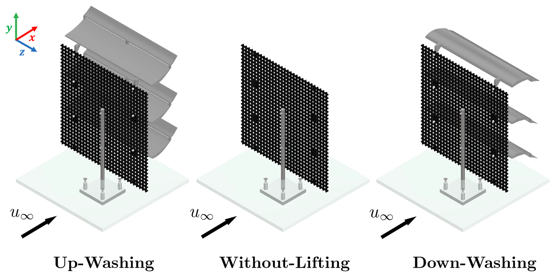
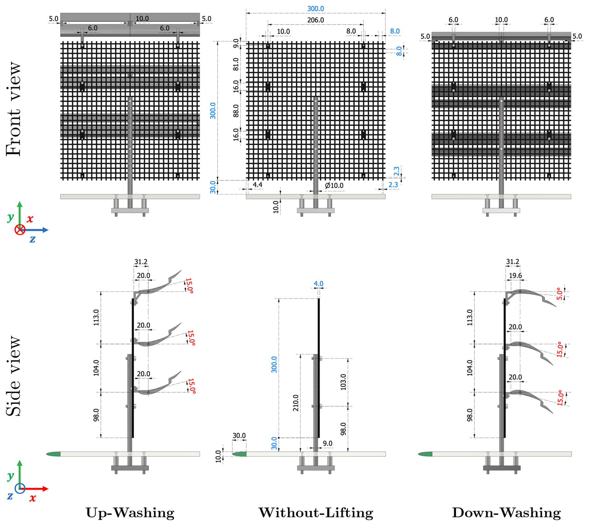
Figure 5 Specifications of the MRSL in different configurations. The top and bottom rows show the front and side views. The left, middle, and right columns correspond to the model representing the Up-Washing, Without-Lifting, and Down-Washing configurations, respectively. Critical dimensions are marked in blue, while the pitch angles of the MRSL’s wings (θ_p) are shown in red. Other specifications are labeled in black. All lengths are given in millimeters (mm), and angles are in degrees (°). The green semi-ellipses in the side views represent the profile of the leading edge installed upstream of the flat plates.

The lifting devices of the MRSL in this study consist of three wings. A two-element airfoil profile is selected for the wings due to its relatively high lift coefficient. A detailed rationale for this choice, along with the XY plot of the airfoil geometry, is provided in Appendix B1. The span of each wing matches the side length of the MRSL, denoted as D, and the chord length is set to $c=D/\mathrm{3}$. The wings are fabricated with additive manufacturing (3D printing) using polylactic acid (PLA) and are integrated with supporting structures. These structures include bolting points for attaching themselves to the porous disks, as shown in Fig. 5.

The vertical positions of the wings, defined by the locations of their pitching axes (see Fig. B3), are at 1.05D, 0.67D, and 0.33D above the bottom edge of the MRSL. The wings are located downstream of the porous disk, with a streamwise distance of 0.10D between the pitching axes and the disk. The clearance between the leading edge of the wings and the disk is 0.04D (11 mm). The pitch angles of the wings θ_p are determined based on preliminary experimental tests described in Appendix B2. Those tests show that the MRSL configured with these selected pitch angles is capable of generating lift comparable to the thrust imposed by the porous disk. Li et al. (2025c) have shown that MRSLs are effective when their magnitudes of lift approximately match that of thrust.

The MRSL in this work is held upright by a steel rod having a diameter of 10 mm. The side of the rod in contact with the porous disk is machined flat to ensure a seamless interface, providing a sturdier installation for both the MRSL (porous disk) and the strain gauges (see Sect. 2.4). This machining reduces the rod’s apparent diameter in side view from 10 to 9 mm, as illustrated in Fig. 5. Note that the steel rod is not intended to replicate the aerodynamic effects of a wind turbine tower; its purpose is purely for holding the model. In fact, all the other supporting structures of the multi-rotor system (e.g., scaffolding) are not represented in the current aerodynamic model, and their aerodynamic impacts are therefore not considered.

2.3 Setups of the regenerative wind farm

The floor, representing the sea surface of the regenerative wind farm, is constructed by seven sheets of transparent flat plates (plexiglass), each measuring 244, 122, and 1 cm in length, width, and thickness, respectively. Assembly details are provided in Figs. 6 and 7 for the cases with the aligned wind farm layout and the staggered wind farm layout. These plates are supported by wooden beams resting on a metallic frame (LINOS X95 System) and are positioned approximately 73 cm above the bottom edge of the wind tunnel exit (7 cm above where the wind tunnel begins to converge in width; see Fig. 3). To mitigate flow separation and to reduce turbulence generation, an elliptical profile with an aspect ratio of 3 is added to the leading edge (Hanson et al., 2012). This profile is illustrated in Fig. 5 and is fabricated using additive manufacturing. To fasten the MRSLs to the flat plates, several holes are drilled and secured using sunken bolts, as shown in Fig. 5. Most of the supporting structures for the MRSLs are positioned beneath the flat plates to minimize flow disturbance.

As illustrated in Fig. 6, the RGWFs with the aligned layout include nine available loci for mounting the MRSL, arranged in three rows and three columns. The row spacing Δ_R between these loci is 5D (150 cm), and the column spacing Δ_C of them is 3D (90 cm). The distance from the first-row MRSLs to the leading edge of the flat plates is 2.6D (77 cm). Note that not all the cases utilize all nine loci (see Sect. 2.7).

In terms of the case with staggered wind farm layout, RGWF consists of only two rows of MRSLs, as depicted in Fig. 7. The absolute position of its origin is relocated 5D downstream relative to the aligned cases (see Fig. 6 for reference). This staggered layout is achieved by shifting three of the flat plates of the aligned layout by a distance of D in the lateral direction.

Further detailed dimensions of the RGWF layouts, including the relative positions of the flat plates to the wind tunnel, the locations of the fields of view (FOVs), and other relevant setup details, are also labeled in Figs. 6 and 7. The origin of the RGWF is defined at the top of the porous disk of the first-row center-column MRSL (marked as “⊗” in Figs. 6 and 7), and the x, y, and z directions correspond to the streamwise, vertical, and lateral directions, respectively. The positions of the other key components, such as the cameras, light sources, and traverse system, are shown by a photograph in Fig. 3.

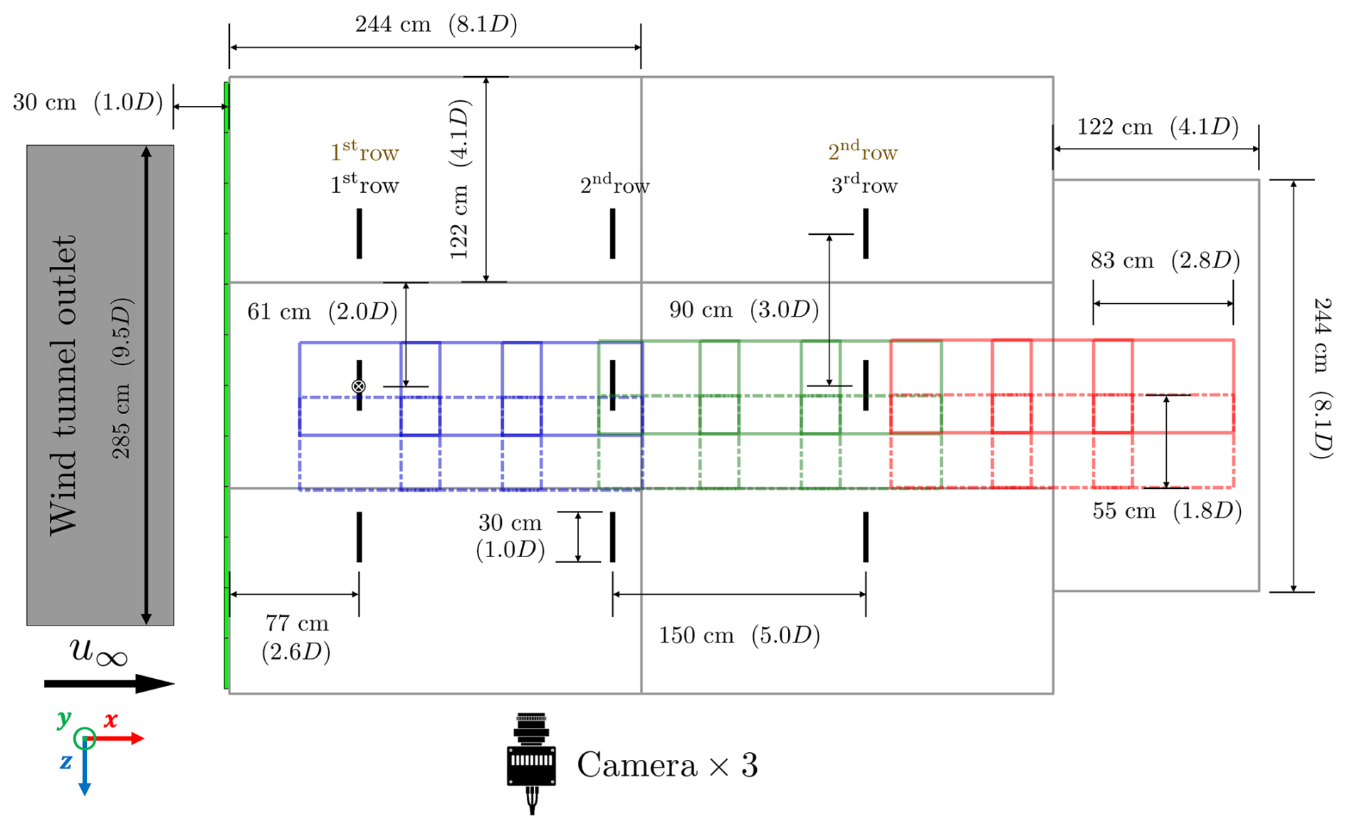
Figure 6 Layout of the experimental setups for the regenerative wind farms, with dimensions labeled. The viewing angle is from above, with the wind being blown from left to right. Seven flat plates (plexiglass), representing the sea surface, are shown as gray rectangles, and the MRSL loci are marked with thick black lines. The origin of the coordinate system, located at the positions of first-row center-column MRSL, is marked with “⊗”. Row numbers are shown in black for cases with Δ_R=5D and in brown for those with Δ_R=10D. The field of views of the 3D-PTV are represented by blue, green, and red rectangles, with the colors corresponding to the three locations of the traverse system (see Sect. 2.8). Elongated green stripes indicate the elliptical leading edges placed in front of the flat plates, and the wind tunnel outlet is shown as a gray block. During the experiment, the cameras are oriented to shoot from the positive z direction.

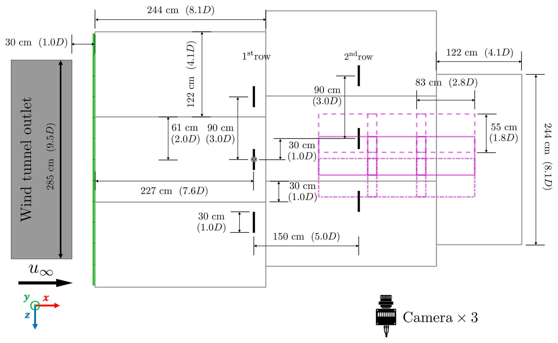
Figure 7 Layout of the experimental setups for regenerative wind farms with dimensions labeled for the staggered case (case UW-05-ST in Table 1). The viewing angle is from above, with the wind being blown from left to right. The origin of the coordinate system, located at the position of the first-row center-column MRSL, is marked with “⊗”. The loci for placing MRSLs are indicated by thick black lines. Magenta rectangles with solid, dashed, and dotted-dashed lines depict the fields of view of the 3D-PTV system.

2.4 Force measurement methodology

To quantify the forces exerted by the MRSLs, both streamwise (thrust of the porous disk and drag of the wings) and vertical (lift of the wings) forces are measured for the MRSLs located in the mid-column. Streamwise forces are recorded using two one-component strain gauges (KD24s 10N, ME-Meβsysteme), which are capable of measuring tensile and compressive loads with a precision of 0.01 N. Vertical forces are measured using a bench scale (FKB 6K0.02, KERN) with a precision of $\mathrm{1}\times {\mathrm{10}}^{-\mathrm{3}}$ N. The measurement duration is about 30 s for both forces. Sampling frequencies are around 1000 Hz for the streamwise forces and 1 Hz for the vertical force.

Since the aerodynamic forces on the disk and wings are coupled, measurements are conducted both with the wings attached and detached, as illustrated in Fig. 8. Notably, the wing holders shown on the right side of Fig. 8 do not contact either the porous disk or the flat plates. Additional holes are drilled on the flat plates for this purpose and are taped when not in use. By subtracting the streamwise forces measured in the two setups, the thrust from the disk and the drag from the wings can be determined separately, despite their aerodynamic coupling. The integration of force measurement devices into the wind farm setup is also shown in Fig. 2. Note that these force measurement devices are removed when measuring the flow fields.

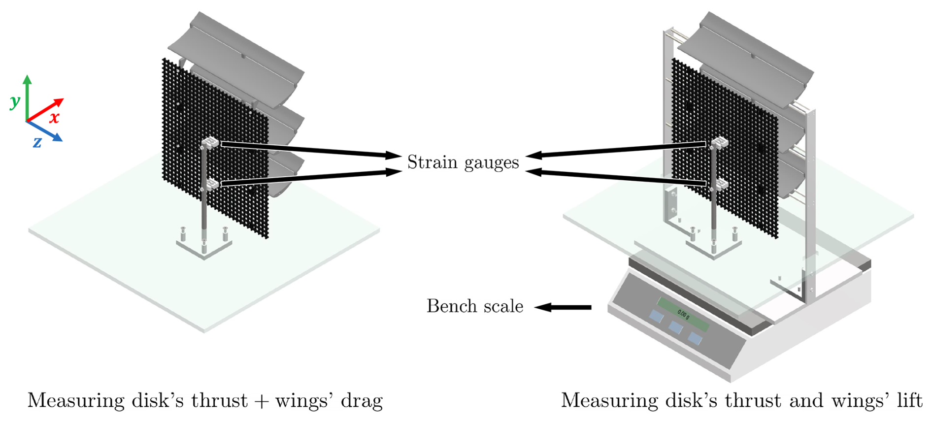
Figure 8 Setups for measuring the forces exerted by the MRSL. Left: configuration for measuring the total streamwise force, comprising the disk’s thrust (T^R) and the wings’ drag (D^W). Right: configuration for concurrently measuring the disk’s thrust (T^R) and the wings’ lift (L^W). Note that the wings’ drag (D^W) is not captured in the right-hand setup, as the wings are detached from the porous disk.

In this work, the thrust (streamwise force) exerted by the porous disk (rotor), the lift (vertical force) exerted by the wings, and the drag (streamwise force) exerted by the wings are denoted as T^R, L^W, and D^W, respectively. For consistency, the positive directions for T^R, L^W, and D^W are defined as negative x, positive y, and negative x, respectively.

The normalized forces, denoted as ${\widehat{T}}^R$, ${\widehat{L}}^{\mathrm{W}}$, and ${\widehat{D}}^{\mathrm{W}}$, are defined in Eq. (1), where the hat operator ($\widehat{\cdot }$) indicates the normalization. The normalization is performed by dividing the measured forces by the reference thrust T^R measured at the mid-column of the first-row MRSL in case WL-05, denoted as $T^{\mathrm{R}}{|}_{\mathrm{1}\mathrm{st}}^{\mathrm{WL}\text{-}\mathrm{05}}$. The value of $T^{\mathrm{R}}{|}_{\mathrm{1}\mathrm{st}}^{\mathrm{WL}\text{-}\mathrm{05}}$ used in this study is 2.07 N, corresponding to a thrust coefficient C_T of 0.72. The definition of C_T employed in this work is provided in Eq. (2), with u_∞=7.3 m s⁻¹ and ρ=1.205 kg m⁻³, which are based on the readings of the wind tunnel facility.

$$\begin{array}{}\text{(1)}& {\displaystyle }\begin{array}{rl}& {\widehat{T}}^{\mathrm{R}}\stackrel{\Delta }{=}{\displaystyle \frac{T^{\mathrm{R}}}{T^{\mathrm{R}}{|}_{\mathrm{1}\mathrm{st}}^{\mathrm{WL}\text{-}\mathrm{05}}}},{\widehat{L}}^{\mathrm{W}}\stackrel{\Delta }{=}{\displaystyle \frac{L^{\mathrm{W}}}{T^{\mathrm{R}}{|}_{\mathrm{1}\mathrm{st}}^{\mathrm{WL}\text{-}\mathrm{05}}}},\\ & {\widehat{D}}^{\mathrm{W}}\stackrel{\Delta }{=}{\displaystyle \frac{D^{\mathrm{W}}}{T^{\mathrm{R}}{|}_{\mathrm{1}\mathrm{st}}^{\mathrm{WL}\text{-}\mathrm{05}}}}\end{array}\text{(2)}& {\displaystyle }{C}_{\mathrm{T}}\stackrel{\Delta }{=}{\displaystyle \frac{T^{\mathrm{R}}}{\mathrm{0.5}\mathit{\rho }{u}_{\mathrm{\infty }}^{\mathrm{2}}{D}^{\mathrm{2}}}}\end{array}$$

2.5 Flow measurement methodology

This study employs three-dimensional particle tracking velocimetry (3D-PTV) to measure flow quantities based on particle trajectories obtained through the imaging system. The PTV system consists of three high-speed cameras (Photron Mini AX100) for imaging and arrays of light-emitting diodes (LED-Flashlight 300 blue, LaVision GmbH) for illumination. Both the cameras and the light source are mounted on a traverse system, as shown in Fig. 3. This allows the PTV system to scan through the RGWF. Neutrally buoyant helium-filled soap bubbles (HFSBs) are used as flow tracers. The flow traces are dispensed by an in-house-developed seeding system, and their median diameter is approximately 300 to 400 µm (Scarano et al., 2015; Faleiros et al., 2019). With the current setup, the field of view (FOV) for a single volume is approximately 830, 550, and 880 mm, corresponding to 2.8, 1.8, and 2.9D in the streamwise, lateral, and vertical directions, respectively. This setup gives a resolution of 0.85 mm px⁻¹. For each measurement, 3000 images are captured with the cameras operating at 1000 Hz. Further details about the 3D-PTV specifications and setup are provided in Appendix A.

2.6 Image processing for flow field quantities

The general procedure for image processing to quantify the flow fields is outlined as follows. First, a subtract-average time filter with a window of 11 time steps is applied to the raw images to reduce noise. Next, particle tracks are extracted from the filtered images using the Shake-the-Box (STB) algorithm (Schanz et al., 2016). The resulting tracks are then binned onto a Cartesian grid to convert the Lagrangian data into Eulerian fields. Finally, the binned Eulerian fields from each measurement volume are stitched together to construct a complete flow field of the RGWF. Detailed descriptions of each step are provided in the remainder of this subsection.

2.6.1 Particle tracking

Three passes are used when performing the STB algorithm to reconstruct the particle tracks, which are forward in time, backward in time, and reconnection of interrupted tracks. With this setup, the number of the active tracks per volume at a time instant ranges from 4000 to 20 000. The variability The variability in track count is primarily due to the blockage of MRSLs, both optically (obstructing the line of sight) and physically (blocking the seedings).

2.6.2 Binning and uncertainty

Once the particle tracks are obtained, they are binned onto a Cartesian grid to compute the spatiotemporal statistics of the flow fields. The binning window consists of $\mathrm{16}\times \mathrm{16}\times \mathrm{16}$ cubic voxels ($\mathrm{11.2}\times \mathrm{11.2}\times \mathrm{11.2}$ mm³) with 50 % overlap. Spatial fitting is performed using a 2nd-order polynomial as advised by Agüera et al. (2016). Tracks shorter than 10 time steps are excluded from the analysis, and no time filtering is applied.

In general, the particle count N per bin exceeds 1000. However, in regions near the MRSL models and in swirling flow areas, the particle count may drop to 300 or fewer. The expanded uncertainty at a 95 % confidence level of the mean velocity, denoted as $|\stackrel{\mathrm{‾}}{\mathit{u}}{|}_{{\mathit{\epsilon }}_{\mathrm{95}}}$, is defined in Eq. (3) (Sciacchitano and Wieneke, 2016). As shown in Fig. 9, in regions that are not significantly influenced by the MRSL, $|\stackrel{\mathrm{‾}}{\mathit{u}}{|}_{{\mathit{\epsilon }}_{\mathrm{95}}}/u_{\mathrm{\infty }}$ is typically well below 1 %. In contrast, in the wake regions, the uncertainty is substantially higher, primarily due to the reduced particle count N. This effect is particularly pronounced in cases with the without-lifting configuration, where tracers are partially blocked by the porous disks and the replenishment is limited due to weaker mixing. Nevertheless, $|\stackrel{\mathrm{‾}}{\mathit{u}}{|}_{{\mathit{\epsilon }}_{\mathrm{95}}}/u_{\mathrm{\infty }}$ generally remains below 5 %, indicating that the obtained statistics have converged.

$$\begin{array}{}\text{(3)}& |\stackrel{\mathrm{‾}}{\mathit{u}}{|}_{{\mathit{\epsilon }}_{\mathrm{95}}}\stackrel{\Delta }{=}{Z}_{\mathrm{95}}\times {\displaystyle \frac{\sqrt{{\mathit{\sigma }}_u^{\mathrm{2}}+{\mathit{\sigma }}_v^{\mathrm{2}}+{\mathit{\sigma }}_w^{\mathrm{2}}}}{\sqrt{N}}},Z_{\mathrm{95}}=\mathrm{1.96}\end{array}$$

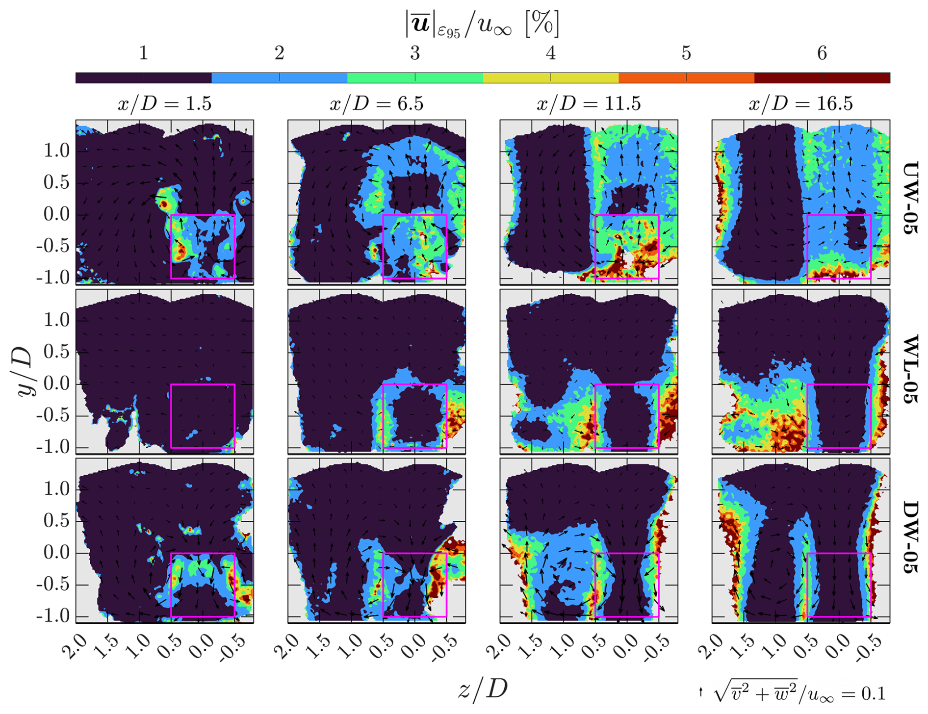
Figure 9 Contours of the uncertainty in the time-averaged velocity magnitude ($|\stackrel{\mathrm{‾}}{\mathit{u}}{|}_{{\mathit{\epsilon }}_{\mathrm{95}}}$) for cases with a row spacing of 5D at several x planes. Case labels given in Table 1 are indicated on the right side of each row, and the corresponding x positions are labeled at the top of each column. The projected areas of MRSLs are marked with magenta squares. Arrows indicate the direction of in-plane velocities, with their lengths scaled by the in-plane velocity magnitude. The scaling reference for the arrows is shown at the bottom right of the figure.

2.6.3 Stitching and scaling the flow quantities

Since the region of interest for the RGWF is significantly larger than the 3D-PTV system's FOV, multiple measurement volumes are acquired to cover the entire domain. These volumes are subsequently stitched together to reconstruct the complete flow fields of RGWFs. The stitching process uses a hyperbolic tangent function as a weighting function to smoothly blend the overlapping regions. Additionally, small variations in wind tunnel speed across different volumes are compensated by scaling the flow quantities during the stitching process. A detailed description of the stitching methodology is provided in Appendix C.

After stitching the measured volumes, the total flow field domain for cases with the aligned layout spans $-\mathrm{1.3}<x/D<\mathrm{16.8}$ (streamwise), $-\mathrm{0.8}<z/D<\mathrm{1.9}$ (lateral), and $-\mathrm{1.1}<y/D<\mathrm{1.5}$ (vertical) relative to the defined origin (see Fig. 6). Meanwhile, for the case with the staggered layout, the total flow field domain spans $\mathrm{3.1}<x/D<\mathrm{10.5}$, $-\mathrm{2.7}<z/D<\mathrm{2.2}$, and $-\mathrm{1.1}<y/D<\mathrm{1.5}$ (see Fig. 7).

Finally, to account for the slight velocity differences across experimental cases caused by wind tunnel variability, the stitched flow fields are normalized by a reference volume-averaged $\stackrel{\mathrm{‾}}{u}$, which serves as the inflow wind speed u_∞. For aligned cases, the reference volume is defined as $-\mathrm{0.95}<x/D<-\mathrm{0.60}$, $\mathrm{0.53}<y/D<\mathrm{0.88}$, and $\mathrm{0.84}<z/D<\mathrm{1.20}$, while the reference volume for the staggered cases is $\mathrm{3.77}<x/D<\mathrm{4.14}$, $-\mathrm{1.50}<z/D<-\mathrm{1.22}$, and $\mathrm{0.90}<y/D<\mathrm{1.28}$. For the current measurement, the obtained u_∞ is around 7.3 m s⁻¹.

2.7 Test matrix

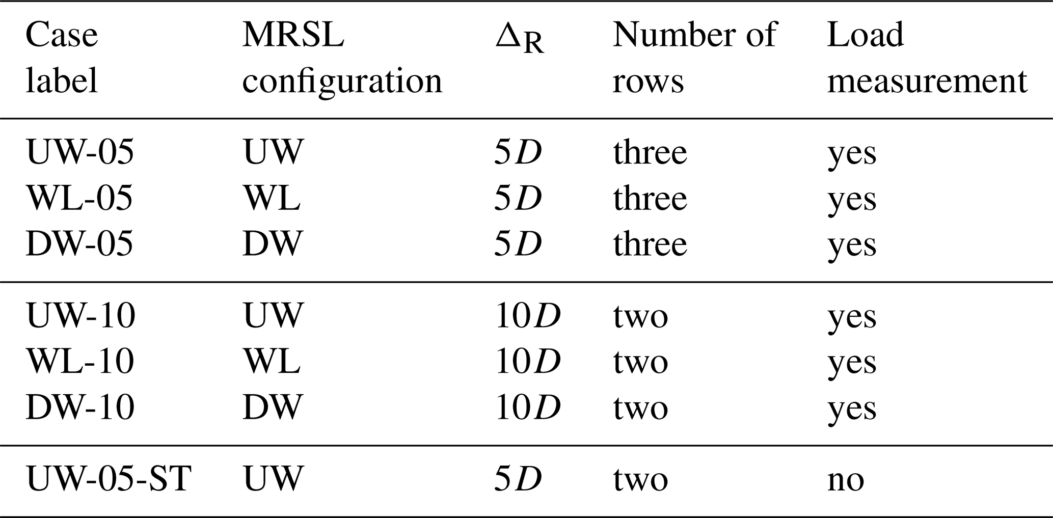
Seven RGWF configurations are tested in this study, and they are listed in Table 1. In this study, RGWFs with three different MRSL configurations are tested with the aligned layout (see Fig. 6), which are Up-Washing (UW), Without-Lifting (WL), and Down-Washing (DW). To better understand the development of the MRSL wakes and to investigate the effect of row spacing Δ_R on MRSL performance, cases with Δ_R=5 and 10D are examined for all three configurations with the aligned wind farm layout (see Fig. 2). Moreover, an additional case with a staggered layout is tested (see Fig. 7), which is case UW-05-ST in Table 1. This case is tested to preliminarily explore the impacts of apparent wind farm layout, such as those caused by varying incoming wind directions in real-world scenarios.

Table 1 Regenerative wind farms tested in this study. The first part of each case label denotes the MRSL configuration, where UW, WL, and DW stand for Up-Washing, Without-Lifting, and Down-Washing, respectively. The two digits in the end/middle indicate the row spacing Δ_R, with 05 and 10 corresponding to 5 and 10D, respectively. The suffix ST stands for staggered, indicating that MRSLs in consecutive rows are not aligned with the inflow direction. For all RGWF configurations, the number of columns is fixed at three, and the lateral spacing between adjacent columns is 3D.

2.8 Procedure of the experiments

This part summarizes the procedures followed during the experimental campaign. Time lapse videos of the experiments demonstrating how the procedure is executed are available in the accompanying data repository (Li et al., 2025a).

When measuring the flow fields of the aligned cases, the traverse system where the PTV system is mounted is initially positioned at the most upstream location, allowing access to the FOVs labeled in blue in Fig. 6. For each RGWF configuration, all FOVs at this traverse position are scanned before reconfiguring the RGWF. This re-configuration involves dismantling and re-installing the MRSLs. After completing all six cases with the aligned wind farm layout in this traverse location, the traverse system is manually moved to the next downstream location, and the same procedure is repeated. This approach minimizes the need for re-positioning and re-calibrating the PTV system, which is relatively more time consuming. In total, three traverse positions are used for the cases with the aligned wind farm layout, requiring two manual re-positions of the traverse system. These three traverse locations correspond to the blue, green, and red FOVs shown in Fig. 6. After completing the flow measurement of all the aligned cases, the case with staggered wind farm layout is tested. For the staggered case, the traverse system remains fixed throughout the measurements, covering the nine magenta FOVs in Fig. 7.

In terms of load measurements, the force-measuring devices are always positioned at the locus in the mid-column of the last row (see Sect. 2.9). MRSLs in the other rows are installed or removed depending on the specific measurement objective. For example, to characterize the forces exerted by an MRSL in the first row, the MRSL of interest is installed at the third-row locus (where the sensors are located), while the MRSLs at the first- and second-row loci are removed. This approach is considered appropriate because the flow field does not exhibit significant variation in the streamwise direction until $x/D>\mathrm{12.0}$, as shown later in Fig. 10. Additionally, since the smallest row spacing used in this study is Δ_R=5D, the influence of downstream MRSLs on the flow conditions experienced by upstream MRSLs is expected to be negligible.

Regarding the duration of the experimental campaign, flow field measurements span approximately 1.5 weeks, while the load measurements are completed within a single day. Note that due to the scheduling constraint of the wind tunnel, only the up-washing configuration is tested for the staggered layout. Also, the force measurements are not conducted for the staggered case for the same reason.

2.9 Flow field characteristics of an empty reference case

To characterize the flow field in the region of interest when all MRSLs are absent, the time-averaged streamwise velocity $\stackrel{\mathrm{‾}}{u}$ measured when all MRSLs are dismounted is presented in Fig. 10. Note that this reference case generally follows the recipe and the procedure introduced earlier. However, to reduce the acquisition time, only 1500 images instead of 3000 are taken per each volume, and the measurements end at $x/D=\mathrm{12}$.

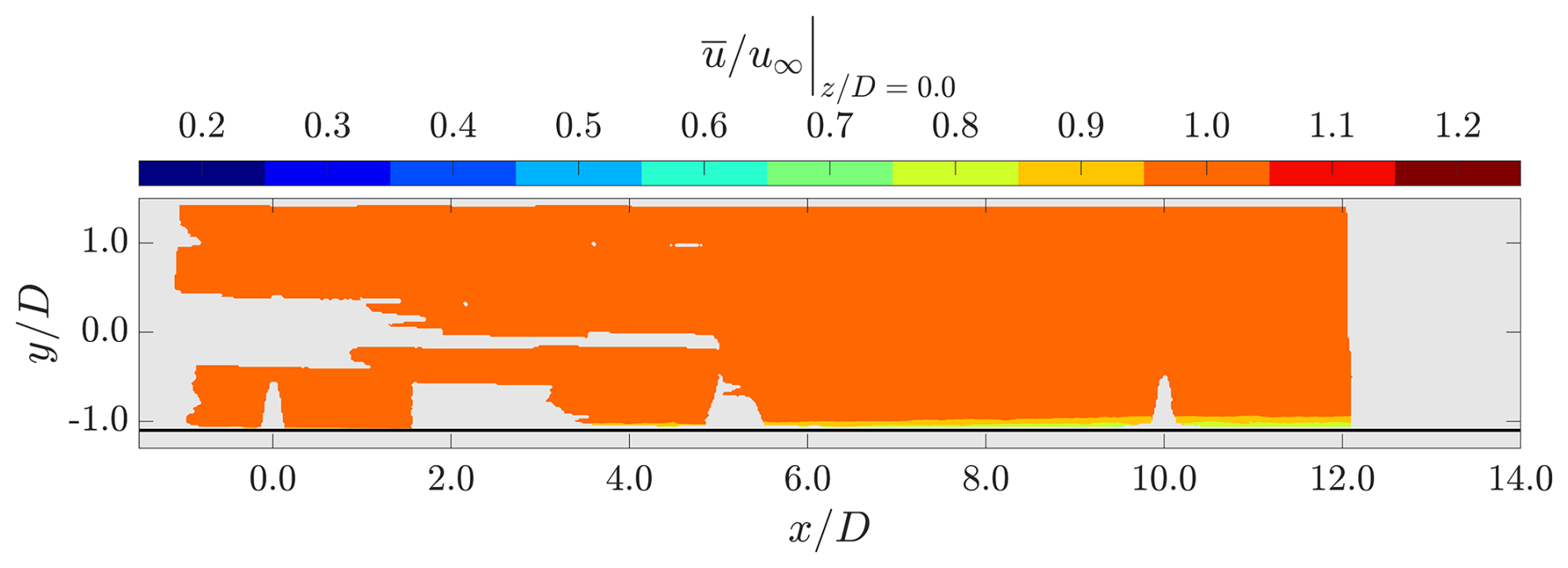
Figure 10 Contours of time-averaged streamwise velocity $\stackrel{\mathrm{‾}}{u}$ when all MRSLs are absent. The value for u_∞ is 7.3 m s⁻¹. The position of the origin and the coordinate system are those given in Fig. 6.

The velocity contour in Fig. 10 shows that the incoming flow while all MRSLs are absent is generally spatially uniform, with minimal vertical velocity shear. Up to at least $x/D=\mathrm{12.0}$, noticeable reductions in $\stackrel{\mathrm{‾}}{u}$ are mostly confined to regions below $y/D=-\mathrm{1.0}$. This indicates that the RGWF's inflow can still be considered as uniform despite the presence of the flat plates, as the growth of the boundary layer is limited. Note that the large areas where data are not available is due to the lack of tracer particles. This limitation is largely alleviated when MRSLs are introduced as the flow tracers are better dispersed by them.

3 Results and discussions

First, Sect. 3.1 focuses on the load measurement results. Next, Sect. 3.2 to 3.4 examines the flow fields through contour plots, where streamwise velocity, turbulence level, and streamwise vorticity are studied. Then, Sect. 3.5 investigates the integral wake characteristics using area-averaged available power. Later on, Sect. 3.6 provides a detailed analysis of the wake recovery mechanisms and compares the present experimental findings with prior numerical studies, enabling cross-comparison and cross-validation. Finally, Sect. 3.7 briefly explores the scenario in which MRSLs in adjacent rows are staggered with respect to the inflow direction.

3.1 Forces exerted by MRSLs

This subsection presents the forces exerted by the MRSLs located in the mid-column. The definitions of the forces and the measurement methodology are described in Sect. 2.4 and 2.8.

3.1.1 Cases with row spacing being 5D

The results for the normalized thrust of the porous disk ${\widehat{T}}^{\mathrm{R}}$, the normalized lift of the wings ${\widehat{L}}^{\mathrm{W}}$, and the normalized drag of the wings ${\widehat{D}}^{\mathrm{W}}$ for the cases with a row spacing of Δ_R=5D are presented in Fig. 11. It is found that T^R measured at the second and third rows are approximately tripled in cases UW-05 and DW-05 compared to case WL-05, despite the presence of additional drag (D^W). These increases are even more pronounced than the numerical results reported by Li et al. (2025c), who found that T^R downstream of the second row approximately doubled with the inclusion of lifting devices. It is important to note, however, that the experiments in this study are conducted under near-laminar inflow conditions with a uniform velocity profile, while the simulations in Li et al. (2025c) applied an inflow turbulence intensity of 8 % and a vertical velocity shear; in addition, their Δ_R was 6D instead of 5D.

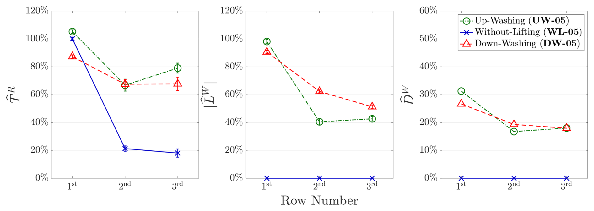
Figure 11 Normalized (time-averaged) rotor's thrust (${\widehat{T}}^{\mathrm{R}}$), wings' lift (${\widehat{L}}^{\mathrm{W}}$), and wings' drag (${\widehat{D}}^{\mathrm{W}}$) for cases with row spacing being 5D. The measured standard deviations for ${\widehat{T}}^{\mathrm{R}}$ and ${\widehat{L}}^{\mathrm{W}}$ are labeled with the error bars. The case labels corresponding to Table 1 are indicated in the legends.

According to classic actuator disk theory (Manwell et al., 2010), tripling the thrust force T^R implies that the power extracted by MRSLs increases by more than a factor of 5. This is based on the relations that $T^{\mathrm{R}}\propto u_{\mathrm{\infty }}^{\mathrm{2}}$ and $P^{\mathrm{R}}\propto u_{\mathrm{\infty }}^{\mathrm{3}}$, where P^R represents the power harvested by the MRSL. The present results therefore indicate that the energy extracted by the MRSLs positioned in the second and third rows are increased around 400 % through the integration of the lifting devices. This substantial enhancement highlights the fact that RGWFs could be much more land efficient than the conventional wind farms – that is, RGWFs are able to output significantly more power with a given unit sea surface.

In addition to the substantial gains in T^R, several aerodynamic characteristics of MRSLs and RGWFs are noteworthy. As shown in Fig. 11, the ratio of lift to thrust ($L^{\mathrm{W}}/T^{\mathrm{R}}$) is approximately 100 % in the first row for cases UW-05 and DW-05, indicating that the MRSLs perform as intended (see Sect. 2.2). However, this ratio gradually decreases in the second and third rows. This reduction is attributed to the vertical flow induced by upstream MRSLs, which modifies the inflow conditions for those of the downstream ones. Specifically, the induced vertical velocity alters the effective angle of attack α experienced by the MRSL's wings, while the pitch angle θ_p of each wing remains fixed regardless of its position in the RGWF (see Sect.  2.2). This observation suggests that to maintain consistent aerodynamic performance, the MRSL's wings should either incorporate adjustable pitch mechanisms or be designed to remain effective across a range of α. Furthermore, in case UW-05, the values of T^R, L^W, and D^W in the third row exceed those in the second row, indicating that wake recovery effects accumulate as the flow progresses deeper into RGWFs. A similar trend is reported in the simulations of Li et al. (2025c). Finally, the error bars in Fig. 11 show that the fluctuations (standard deviations) of T^R increase in the downstream rows, reflecting the growing influences of turbulence generated by the MRSLs located upstream.

Another notable observation is that the first-row MRSL of the up-washing configuration exhibits the highest T^R among the three configurations, followed by without-lifting and then down-washing. This result can be attributed to the bound circulation system generated by the top wings of the MRSL. According to classic airfoil theory, the flow over the suction side of an airfoil accelerates, while the flow over the pressure side decelerates (Anderson, 2011). As a result, in the up-washing configuration, the upper region of the MRSL experiences increased flow velocity, enhancing the thrust generated. Conversely, in the down-washing configuration, the deceleration caused by the pressure side reduces the flow velocity through the upper part of the MRSL, resulting in lower T^R. This effect has also been observed in prior numerical simulations by Li et al. (2025b) and Li et al. (2025c), and is further explored in Appendix B2.

3.1.2 Cases with row spacing being 10D

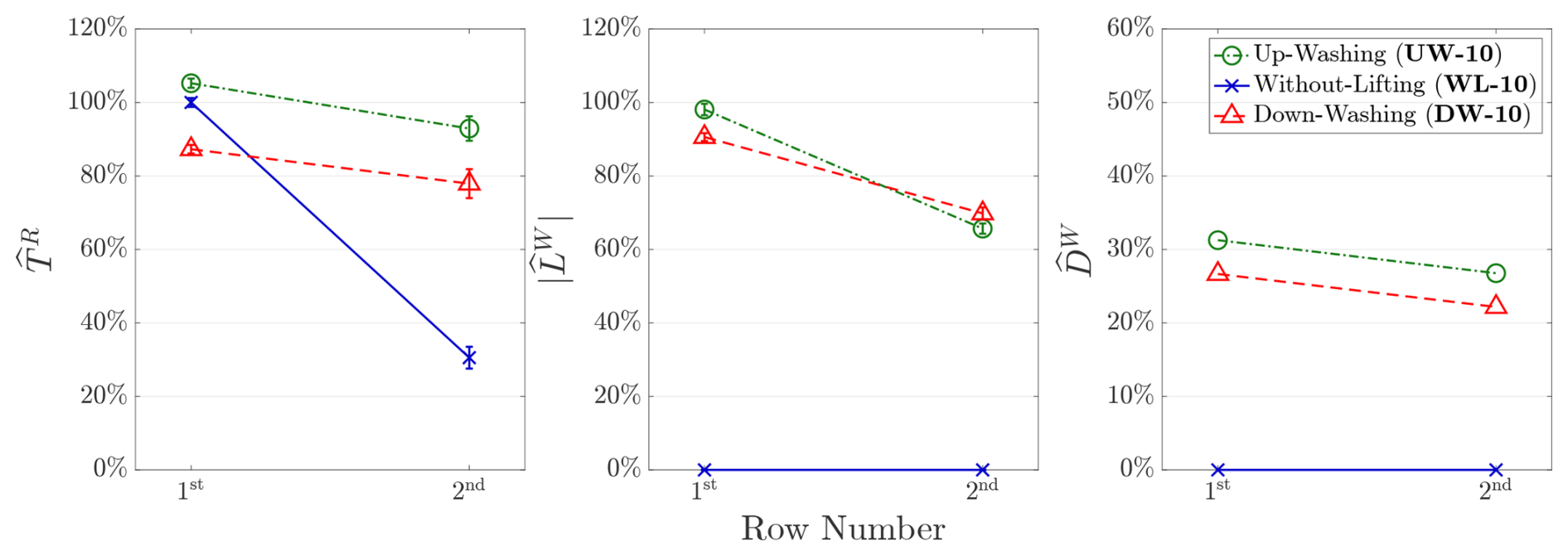
To investigate whether the effects of lifting devices are still significant in regenerative wind farms with larger row spacing, cases with Δ_R=10D are tested, namely cases UW-10, WL-10, and DW-10 in Table 1. The results of the forces exerted in these cases are presented in Fig. 12. It is evident that the cases with lifting devices (UW-10 and DW-10) continue to substantially outperform the case without lifting devices (WL-10), demonstrating that the proposed concept remains effective with larger Δ_R. Moreover, the second-row MRSLs in the cases with Δ_R=10 exert stronger forces compared to the second-row MRSLs with Δ_R=5D across all three configurations. These results suggest that larger row spacing allows more wake recovery, which is an outcome consistent with the field measurements (Barthelmie et al., 2010).

Figure 12 Normalized (time-averaged) rotor's thrust (${\widehat{T}}^{\mathrm{R}}$), wings' lift (${\widehat{L}}^{\mathrm{W}}$), and wings' drag (${\widehat{D}}^{\mathrm{W}}$) for cases with row spacing being 10D. The measured standard deviations for ${\widehat{T}}^{\mathrm{R}}$ and ${\widehat{L}}^{\mathrm{W}}$ are labeled with the error bars. The case labels corresponding to Table 1 are indicated in the legends.

3.2 Time-averaged streamwise velocity

Contours of the time-averaged streamwise velocity $\stackrel{\mathrm{‾}}{u}$ are presented in Figs. 13 and 14, where Fig. 13 corresponds to cases with Δ_R=5D and Fig. 14 corresponds to cases with Δ_R=10D. In addition to the plane $z/D=\mathrm{0}$, several x planes are included to provide a holistic three-dimensional view of the flow fields. The direction and relative magnitude of the in-plane velocities are qualitatively illustrated using arrows. Additionally, to provide more precise illustrations, planar views of the $\stackrel{\mathrm{‾}}{u}$ fields at various x planes for cases with Δ_R=5D are provided in Fig. 15. For a more comprehensive set of velocity contours, including those for the time-averaged vertical velocity $\stackrel{\mathrm{‾}}{v}$, readers are referred to the work of Fijen (2025).

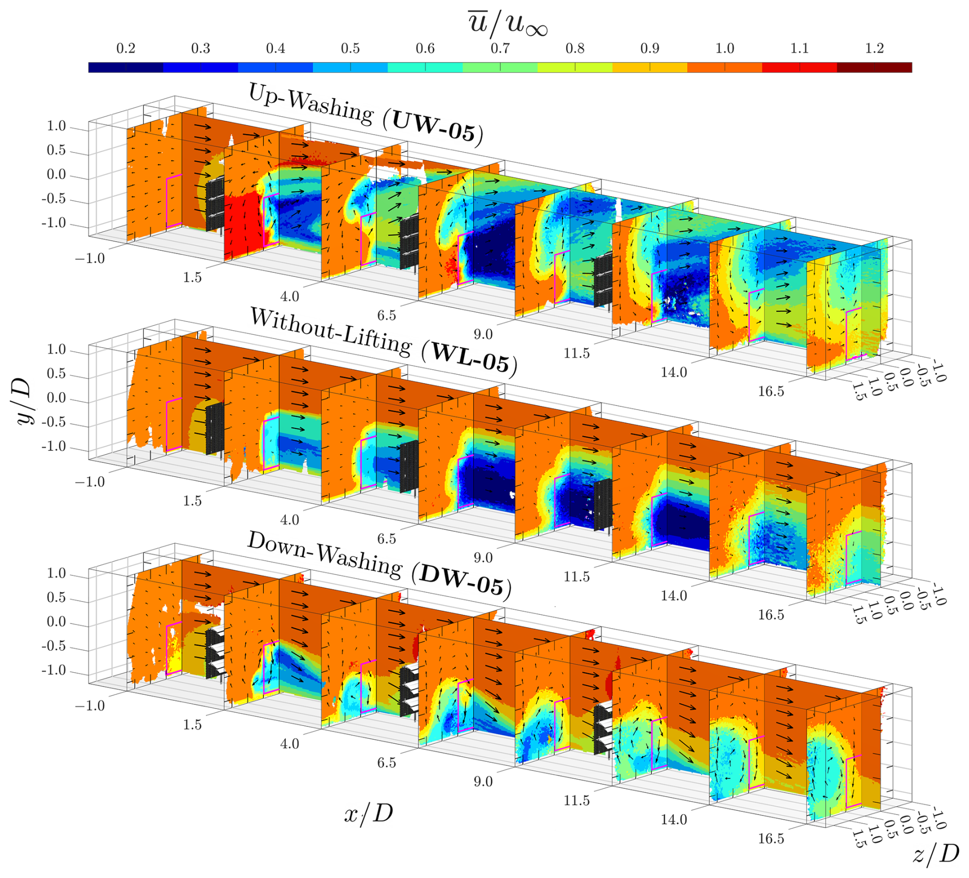
Figure 13 Holistic view of the time-averaged streamwise velocity ($\stackrel{\mathrm{‾}}{u}$) fields for cases with a row spacing of 5D, where MRSLs are positioned at $x/D=\mathrm{0.0}$, 5.0, and 10.0. The projected areas of the MRSLs are marked with magenta squares. Arrows indicate the direction of in-plane velocities, with their lengths scaled according to the in-plane velocity magnitudes. Note that no reverse flow is observed. The minimum values of $\stackrel{\mathrm{‾}}{u}/u_{\mathrm{\infty }}$ in cases UW-05 and WL-05 are approximately 0.1 and 0.2, respectively.

Starting with the inflow conditions at the $x/D=-\mathrm{1.0}$ plane, all three cases exhibit uniform inflow. Additionally, a deceleration in the streamwise velocity is observed directly upstream of the first-row MRSLs, caused by the induction effect of the porous disks. This behavior is consistent with previous experimental findings (Lignarolo et al., 2016), further supporting the validity of the measured velocity fields.

Downstream of the first-row MRSLs, regions of velocity deficit (commonly referred to as wakes) are clearly observed. A comparison of the contours in Figs. 13 and 15 reveals that the three MRSL configurations produce distinctly different wake patterns, indicating that the lifting devices significantly influence wake aerodynamics. Specifically, in the up-washing configuration, the wake is effectively deflected upward as it progresses downstream, while in the down-washing configuration, the wake is steered downward and subsequently spread laterally. These trends persist throughout the measured domain. Consequently, in both UW-05 and DW-05, the regions with the strongest velocity deficit are diverted away from the frontal areas of the second- and third-row MRSLs, enabling those rows to enjoy higher-energized flows that have weaker velocity deficits. In contrast, in WL-05 (without lifting devices), the wake shows minimal vertical or lateral deflection as it is convected downstream, causing the downstream MRSLs to remain fully immersed in the wake of the upstream ones. (The regions with particularly strong velocity deficits observed at $x/D=\mathrm{1.5}$ for WL-05 in Fig. 15 are associated with the wake of the support tower and wing mounting structures.) These flow field observations correlate closely with the force measurements presented in Fig. 11, explaining why the downstream MRSLs in UW-05 and DW-05 significantly outperform those in WL-05.

A closer examination of the in-plane velocities, as depicted by the arrows in Figs. 13 to 15, reveals the presence of strong swirling motions in the cases where MRSLs are equipped with lifting devices. In contrast, these swirling structures are absent in the case without lifting devices. It is these swirls that divert the wakes away from the downstream MRSLs. However, steering the wakes alone is not the ultimate goal of the RGWF. The primary objective is to enhance vertical entrainment by promoting mixing between the wake and the ambient flow above. Based on the presented contours, this goal appears to be successfully achieved. Specifically, the cases with lifting devices exhibit broader regions where $u/u_{\mathrm{\infty }}<\mathrm{0.95}$ and reduced areas where $u/u_{\mathrm{\infty }}<\mathrm{0.15}$, indicating increased wake penetration into the surrounding flow and that the most severe velocity deficits are mitigated. These two indicators collectively demonstrate that the lifting devices effectively enhance vertical mixing and promote wake recovery.

Figure 14 presents the streamwise velocity contours for the three cases with a row spacing of Δ_R=10D. In general, these cases exhibit similar flow characteristics to those with Δ_R=5D, shown in Fig. 13, including the influences of the lifting devices on the wake behaviors. However, the increased spacing allows for the clearer observation of the spatial development of the MRSLs' wakes. Notably, the in-plane velocity vectors indicate that the swirling motions persist at even more than 9D downstream from the MRSLs. This sustained vortical structure highlights the effectiveness of the lifting devices in wake manipulation over long distances, thereby highlighting the efficacy of the RGWF.

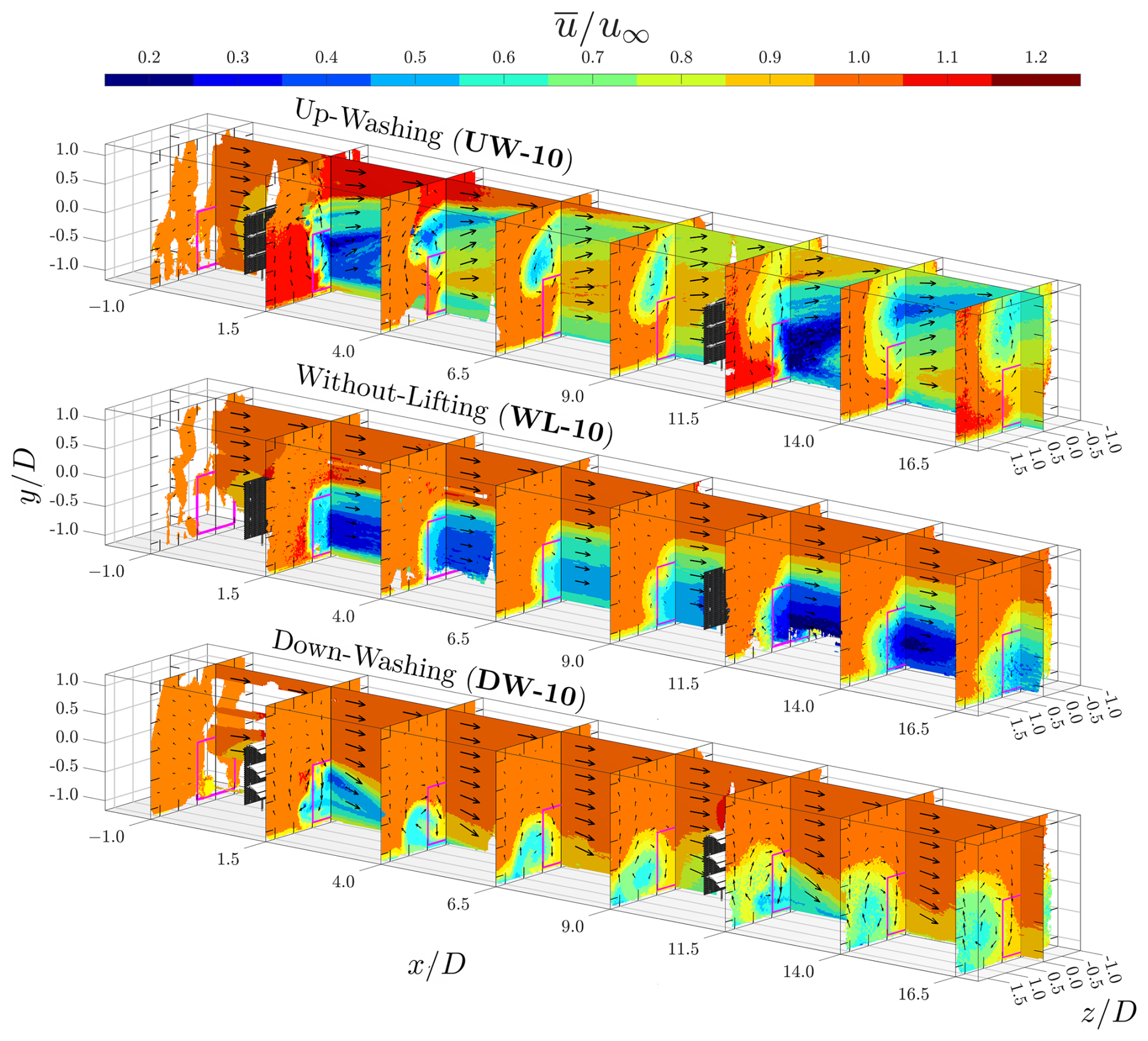
Figure 14 Holistic view of the time-averaged streamwise velocity ($\stackrel{\mathrm{‾}}{u}$) fields for cases with a row spacing of 10D, where MRSLs are positioned at $x/D=\mathrm{0.0}$ and 10.0. The projected areas of the MRSLs are marked with magenta squares. Arrows indicate the direction of in-plane velocities, with their lengths scaled according to the in-plane velocity magnitudes.

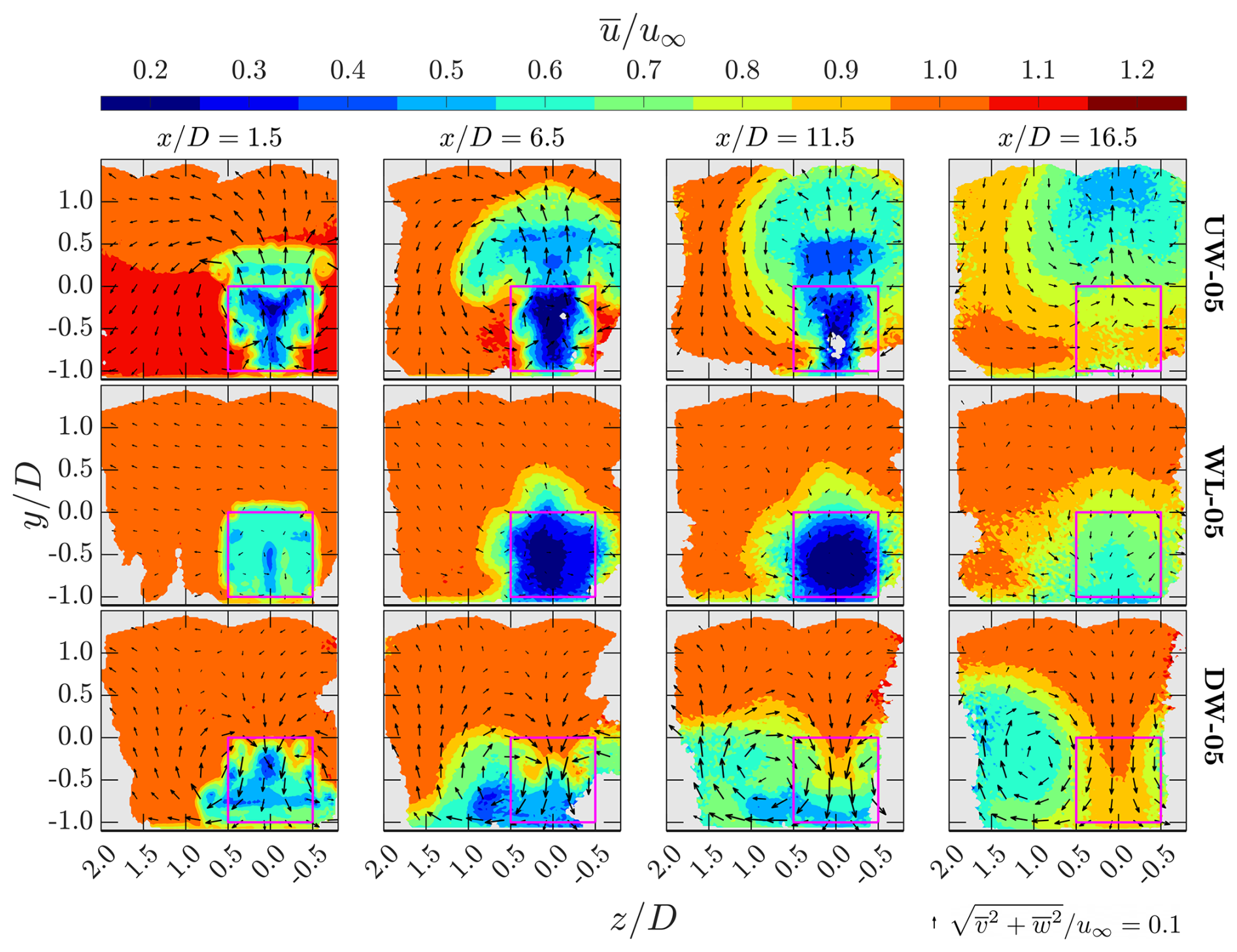
Figure 15 Planar views of the time-averaged streamwise velocity ($\stackrel{\mathrm{‾}}{u}$) for cases with a row spacing of 5D, shown at several x planes. Case labels are indicated on the right side of each row, and the corresponding x positions are labeled at the top of each column. The projected areas of the MRSLs are indicated by magenta squares. Arrows represent the direction of in-plane velocities, with their lengths scaled by their velocity norms. The scaling reference is shown at the bottom right of the figure.

A closer examination of case WL-10 in Fig. 14 reveals a relatively sharp velocity variation at around $x/D=\mathrm{5}$. Note that no MRSL are positioned at that location. This discontinuity can be attributed to the fact that flow data before and after $x/D=\mathrm{5}$ are obtained from separate measurement sessions. Between these sessions, the scaled RGWFs are dismantled and rebuilt, and the traverse system is manually repositioned (see Sect. 2.8). This observation suggests that the primary source of experimental uncertainty is not the velocimetry itself but rather the variability introduced during the reconstruction of RGWFs. A more quantitative assessment is provided in Sect. 3.5. Nevertheless, it is important to point out that these uncertainties have minimal influence on the overall conclusions of this study, as the aerodynamic effects of the lifting devices are sufficiently pronounced to remain clearly distinguishable despite such imperfections.

Lastly, it is worth noting that the velocity contours obtained in this study closely resemble the numerical results reported by Li et al. (2025b) and Li et al. (2025c). This strong agreement not only validates the numerical simulations using experimental data but also consolidates the present experimental findings despite data imperfections. Moreover, through this cross-checking, it is demonstrated that consistent conclusions about RGWFs can be drawn from independent methodologies.

3.3 Turbulence intensity

The contours of turbulence intensity (TI), defined in Eq. (4), are shown in Fig. 16 for cases with Δ_R=5D. TI fields are of particular interest, as turbulence is a dominant factor influencing the fatigue loads experienced by wind turbine systems (Manwell et al., 2010; Watson et al., 2019). Moreover, previous studies have shown that turbulence significantly affects the large-scale coherent structures within wind turbine wakes, often diminishing their influence on downstream wake aerodynamics (Li et al., 2024; Yen et al., 2025). This effect is especially critical for RGWFs, which rely on the preservation of large-scale vortical structures to enhance vertical energy entrainment. Therefore, a thorough understanding of the role of turbulence is essential before pursuing practical implementations of the proposed concept.

$$\begin{array}{}\text{(4)}& \mathrm{TI}\stackrel{\Delta }{=}{\displaystyle \frac{\sqrt{\mathrm{2}k/\mathrm{3}}}{u_{\mathrm{\infty }}}},k\equiv \mathrm{TKE}\stackrel{\Delta }{=}{\displaystyle \frac{\mathrm{1}}{\mathrm{2}}}\left({\mathit{\sigma }}_u^{\mathrm{2}}+{\mathit{\sigma }}_v^{\mathrm{2}}+{\mathit{\sigma }}_w^{\mathrm{2}}\right)\end{array}$$

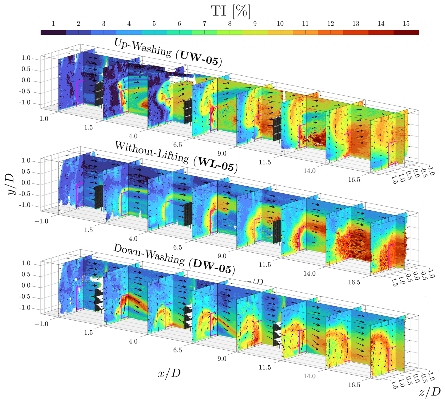
Figure 16 Holistic view of the turbulence intensity (TI) fields for cases with a row spacing of 5D, where MRSLs are positioned at $x/D=\mathrm{0.0}$, 5.0, and 10.0. The projected areas of the MRSLs are marked with magenta squares. Arrows indicate the direction of in-plane velocities, with their lengths scaled according to the in-plane velocity magnitudes.

In general, the turbulence levels are observed to progressively increase as the flow passes through successive rows of MRSLs, consistent with findings from conventional wind turbine arrays (Wu and Porté-Agel, 2015). Specifically, prior to entering the domain of RGWF, the freestream turbulence intensity are found to be around 2 % based on the values reported at $x/D=-\mathrm{1.0}$. After passing the first and second rows of MRSLs, TI exceeds 10 % at $x/D=\mathrm{4.0}$ and reaches over 12% at $x/D=\mathrm{9.0}$, surpassing typical offshore TI levels, which range from approximately 5 % to 8 % (Hansen et al., 2012).

Notably, vertical flows induced by the lifting devices remain significant beyond $x/D=\mathrm{9.0}$ for cases with Δ_R=5D despite the presence of high levels of turbulence in this region, which can be seen in Fig. 13. This indicates that the effectiveness of the MRSLs persists even under highly turbulent conditions. Furthermore, based on the thrust results in Fig. 11, the performance of the third-row MRSLs equipped with lifting devices remains substantially higher than that of the configuration without lifting devices. This implies that the vertical energy entrainment between the second and third rows is still significantly enhanced by the lifting devices despite the second-row MRSLs being subjected to highly turbulent flows. These experimental findings support the numerical results of Li et al. (2025b), who reported that inflow turbulence has minimal impact on the aerodynamic performance of MRSL lifting devices. While the current results preliminarily show that the MRSL concept is relatively insensitive to ambient turbulence levels, further experiments with controlled inflow turbulence are necessary to obtain more quantitative insights.

Furthermore, Fig. 16 reveals several features of the MRSL wake structures. Specifically, three sets of regions exhibiting elevated turbulence intensity are identified. The first set corresponds to the wake edges, which is attributed to the strong velocity shear (Wu and Porté-Agel, 2011). The second set are the regions of the swirling centers, which are clearly visible when examining the TI contours in Fig. 16 alongside the vorticity contours in Fig. 17. These strong velocity fluctuations are due to the instabilities of the tip vortices (Giuni and Green, 2013). The third set of regions corresponds to the wakes of the wings, most clearly observed in case UW-05 as three distinct strips with high values of TI can be identified on the $z/D=\mathrm{0.0}$ plane near $x/D=\mathrm{2.5}$. These high-TI strips result from the shear layer instabilities developed along and after the wings (Wang and Ghaemi, 2022). In general, the locations and characteristics of these high-TI regions are consistent with prior findings on the general features of wake flow, which reinforce the validity of the present experimental results.

3.4 Time-averaged streamwise vorticity

This section examines the vorticity fields to investigate the tip vortices generated by the lifting devices of MRSLs. These vortical structures are closely associated with the swirling motions previously observed in Figs. 13 and 14. Contours of the time-averaged streamwise vorticity ${\stackrel{\mathrm{‾}}{\mathit{\omega }}}_x$ at several x planes for cases with Δ_R=5D are presented in Fig. 17.

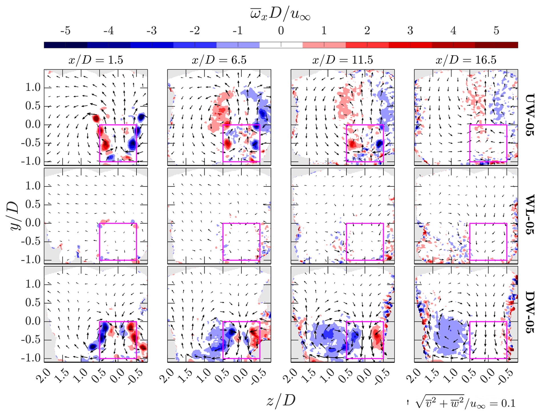
Figure 17 Contours of time-averaged streamwise vorticity (${\stackrel{\mathrm{‾}}{\mathit{\omega }}}_x$) for cases with a row spacing of 5D at several x planes. Case labels are indicated on the right side of each row, and the corresponding x positions are labeled at the top of each column. The projected areas of the MRSLs are marked with magenta squares. In-plane velocity directions are illustrated by arrows, scaled according to their magnitudes. The reference scale for the arrows is provided in the bottom-right corner of the figure. Note that the data have been filtered by spatial averaging over a spherical volume, with a radius of 0.06D.

To reduce noise in the vorticity fields, the data are spatially filtered by averaging over a spherical volume with a radius of 0.06D, which is three times the binning size. The averaging is weighted by the particle count N. This filtering procedure is applied only in this section and in Sect. 3.6, where contours of spatial derivatives are studied.

In Fig. 17, no significant vortical structures are observed throughout the RGWF in the case without lifting devices (WL-05). This outcome is expected, as no significant circulations are induced.

In the up-washing case (UW-05), three pairs of tip vortices generated by the wings of the first-row MRSL are clearly identifiable at $x/D=\mathrm{1.5}$. By $x/D=\mathrm{6.5}$, these tip vortices have diffused, forming broader regions of vorticity with reduced magnitude. At the same streamwise location, three new pairs of tip vortices released by the wings of the second-row MRSL can be observed, overlapping onto the remnants vortices of the first-row MRSL. This observation supports the findings of Li et al. (2025c), who reported that the circulation system within RGWFs can be accumulated through successive rows of MRSLs. At $x/D=\mathrm{11.5}$, the individual tip vortices from the third-row MRSL become less distinguishable, with only the vortices from the bottom wing remaining clearly outlined. Besides the accumulated turbulence within the wind farm (see Fig. 16), this degradation may also result from the drop in L^W due to the strong vertical flow induced by the upstream MRSLs, which makes the downstream MRSLs operate at off-design conditions as changes in the angle of attack are significant (see the in-plane velocity vectors in Fig. 17). As stated in Sect. 3.1, this finding again suggests that the effectiveness of MRSL lifting devices could be further improved by enabling the active control of wing pitch angles or by applying the wings that are less sensitive to variations in angle of attack. By $x/D=\mathrm{16.5}$, the streamwise vortical structures have largely dissipated, which is largely ascribed to the large turbulent fluctuations downstream of the third row, as shown in Fig. 16.

In the down-washing case (DW-05), the tip vortices from the three wings of the first-row MRSL are clearly visible at $x/D=\mathrm{1.5}$, similar to those observed in the up-washing case. As with UW-05, the vortices from the second-row MRSLs overlap with the diffused vortical structures originating from the first row. Interestingly, unlike the up-washing configuration, the tip vortices from all three wings of the third-row MRSLs in case DW-05 remain identifiable at $x/D=\mathrm{11.5}$. Moreover, at $x/D=\mathrm{11.5}$ and 16.5, the vortical structures in the down-washing case appear to be stronger than those in the up-washing case. The underlying cause of this difference is not explored in the present study. One plausible explanation is the higher lift forces ($\left|L^{\mathrm{W}}\right|$) generated by the MRSLs in the second and third rows of DW-05 compared to those in UW-05. Another possibility is the presence of the floor, which may interact more intensively with the downward-directed wake and thereby affect the vortical structures.

Another aspect worth highlighting is the vertical positions of the swirling centers. In the up-washing case, the swirling centers extend from around the center of the MRSL projection area ($y\simeq -\mathrm{0.5}$) upward into the higher regions ($y/D>\mathrm{0.5}$) as the flow progresses deeper into the RGFW. This behavior is closely linked to the self-propelling nature of vortex pairs released by MRSLs, which is elaborated on in the work of Avila Correia Martins et al. (2025) and has also been reported by Li et al. (2025c) and Li et al. (2025b). In contrast, for the down-washing case, the swirling centers remain confined below the top of MRSLs. This distinction may make the up-washing configuration more favorable than the down-washing configuration, given that the primary objective of MRSL and RGWF is to enhance vertical energy entrainment. As illustrated with the velocity vectors in Figs. 13 and 17, compared to the down-washing configuration, the up-washing configuration demonstrates a greater capacity to mix the MRSL wake with the higher-altitude flow.

A more comprehensive set of contour plots and three-dimensional iso-surfaces of ${\stackrel{\mathrm{‾}}{\mathit{\omega }}}_x$ for cases with Δ_R=5D are provided in Appendix D, where the vortex dynamics of the MRSLs are illustrated in greater detail. In particular, the spatial evolution of the vortical structures between successive rows is explicitly illustrated and discussed. In addition, contour plots of ${\stackrel{\mathrm{‾}}{\mathit{\omega }}}_x$ for cases with Δ_R=10D are available in Fijen (2025).

3.5 Available power based on the frontal projection area

Before starting the analysis, the usage and the explanation of the subscript $\widehat{z}$ is provided. The subscripts $\widehat{z}$ in this work indicate that the properties are averaged over two points that are opposite with respect to the symmetry plane $z/D=\mathrm{0}$, as mathematically expressed by Eq. (5). This in fact corresponds to mirroring the half of the flow field across the symmetry plane $z/D=\mathrm{0}$ and averaging it with the another half of the flow fields. The ± sign in the equation becomes minus only when property B is the z component of a vector. Note that when averaging the experimental data, the data are weighted by the particle counts N. Moreover, N=0 is set if the data point is not available (NaNs).

$$\begin{array}{}\text{(5)}& \begin{array}{rl}& \mathrm{For}\mathrm{property}B(x,y,z):\\ & B_{\widehat{z}}(x,y,\widehat{z})\stackrel{\Delta }{=}\\ & {\displaystyle \frac{N(x,y,\widehat{z})\times B(x,y,\widehat{z})\pm N(x,y,-\widehat{z})\times B(x,y,-\widehat{z})}{N(x,y,\widehat{z})+N(x,y,-\widehat{z})}}\end{array}\end{array}$$

Figure 18 presents the available power averaged over the MRSL's frontal projection area, denoted as $<{\stackrel{\mathrm{‾}}{u}}_{\widehat{z}}^{\mathrm{3}}{>}_{\mathrm{PA}}$, along the streamwise direction. The definition of $<{\stackrel{\mathrm{‾}}{u}}_{\widehat{z}}^{\mathrm{3}}{>}_{\mathrm{PA}}$ used in this study is provided in Eq. (6). Note that by employing ${\stackrel{\mathrm{‾}}{u}}_{\widehat{z}}$, the influence of unavailable data points (NaNs) is partially mitigated. $<{\stackrel{\mathrm{‾}}{u}}_{\widehat{z}}^{\mathrm{3}}{>}_{\mathrm{PA}}$ is of particular interest because it serves as an indicator of the integral characteristics of the MRSL wake, directly indicating the flow energy available for harvesting. As a result, it is used in this study as a representative metric for evaluating the overall wake recovery rate.

$$\begin{array}{}\text{(6)}& \begin{array}{rl}& <{\stackrel{\mathrm{‾}}{u}}_{\widehat{z}}^{\mathrm{3}}{>}_{\mathrm{PA}}\left(x\right)\equiv <{\stackrel{\mathrm{‾}}{u}}_{\widehat{z}}^{\mathrm{3}}{>}_{\widehat{z}\in [-\mathrm{0.5}D,\mathrm{0.5}D]}\left(x\right),\\ & <{\stackrel{\mathrm{‾}}{u}}_{\widehat{z}}^{\mathrm{3}}{>}_{\widehat{z}\in [a,b]}\left(x\right)\stackrel{\Delta }{=}{\displaystyle \frac{{\int }_a^b{\int }_{-\mathrm{1.0}D}^{\mathrm{0.0}D}{\left[{\stackrel{\mathrm{‾}}{u}}_{\widehat{z}}(x,y,\widehat{z})\right]}^{\mathrm{3}}\mathrm{d}y\mathrm{d}\widehat{z}}{(b-a)D}}\end{array}\end{array}$$

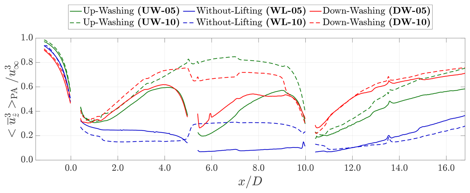
Figure 18 Available power averaged over the frontal projection area $<{\stackrel{\mathrm{‾}}{u}}_{\widehat{z}}^{\mathrm{3}}{>}_{\mathrm{PA}}$ for RGWFs with their MRSLs configured differently. Results are shown for both Δ_R=5D (solid lines) and Δ_R=10D (dashed lines), with case labels corresponding to those introduced in Table 1. MRSLs are located at $x/D=\mathrm{0.0}$, 5.0, and 10.0 for Δ_R=5D, and at $x/D=\mathrm{0.0}$ and 5.0 for Δ_R=10D. The available power is computed using Eq. (6), and the usage of subscript $\widehat{z}$ is defined in Eq. (5).

In Fig. 18, differences in $<{\stackrel{\mathrm{‾}}{u}}_{\widehat{z}}^{\mathrm{3}}{>}_{\mathrm{PA}}$ are already apparent upstream of the first-row MRSLs. For $x/D<\mathrm{0.0}$, the cases with up-washing configuration exhibit higher values of $<{\stackrel{\mathrm{‾}}{u}}_{\widehat{z}}^{\mathrm{3}}{>}_{\mathrm{PA}}$ compared to those with without-lifting configuration, while those with down-washing configuration show the lowest values among the three configurations. These trends are consistent with the thrust forces (T^R) reported in Figs. 11 and 12. Also, the aerodynamic mechanisms that account for the variations in T^R for the first-row MRSLs again explain the observed differences in $<{\stackrel{\mathrm{‾}}{u}}_{\widehat{z}}^{\mathrm{3}}{>}_{\mathrm{PA}}$ at $x/D<\mathrm{0.0}$.

In general, all six cases follow the one-dimensional momentum theory (Manwell et al., 2010), where the $<{\stackrel{\mathrm{‾}}{u}}_{\widehat{z}}^{\mathrm{3}}{>}_{\mathrm{PA}}$ curves decrease with increasing x immediately upstream and downstream of the first-row MRSLs at $x/D=\mathrm{0.0}$. Subsequently, around $x/D=\mathrm{1.0}$, the available power in the up-washing and down-washing cases begins to increase, indicating the onset of wake recovery. In contrast, for without-lifting configuration, $<{\stackrel{\mathrm{‾}}{u}}_{\widehat{z}}^{\mathrm{3}}{>}_{\mathrm{PA}}$ remains nearly constant, suggesting that wake recovery is absent or minimal. The trends in $<{\stackrel{\mathrm{‾}}{u}}_{\widehat{z}}^{\mathrm{3}}{>}_{\mathrm{PA}}$ closely correspond to the velocity fields shown in Figs. 13 and 14, which demonstrate significant wake recovery for up-washing and down-washing cases but not for without-lifting case.

At $x/D=\mathrm{5.0}$ for cases with Δ_R=10D, the available power for cases UW-10 and DW-10 are approximately three to four times greater than that for case WL-10. This trend aligns well with the thrust measurements for the cases with Δ_R=5D, shown in Fig. 11, where the second-row MRSLs equipped with lifting devices exhibit T^R that is around three times of that without.

The profiles of $<{\stackrel{\mathrm{‾}}{u}}_{\widehat{z}}^{\mathrm{3}}{>}_{\mathrm{PA}}$ around the second-row MRSLs for the cases with Δ_D=5D generally follow a similar trend to those at the first-row. A drop in $<{\stackrel{\mathrm{‾}}{u}}_{\widehat{z}}^{\mathrm{3}}{>}_{\mathrm{PA}}$ is again observed immediately upstream and downstream of the second-row MRSLs at $x/D=\mathrm{5.0}$. After the flow passes the second-row MRSLs, the cases with up-washing and down-washing configurations exhibit strong wake recovery, in sharp contrast to the minimal recovery observed in those case with without-lifting.

The profiles of $<{\stackrel{\mathrm{‾}}{u}}_{\widehat{z}}^{\mathrm{3}}{>}_{\mathrm{PA}}$ after the third-row MRSLs for the cases with Δ_D=5D and those after the second-row MRSLs for the cases with Δ_D=10D display similar trends. In general, all profiles show evidence of wake recovery. Notably, even the cases with without-lifting configuration exhibit recovery in these regions, primarily due to the strong turbulent mixing after $x/D=\mathrm{10}$, as shown by fields of turbulence intensity presented in Fig. 16. A closer examination of the slopes of $<{\stackrel{\mathrm{‾}}{u}}_{\widehat{z}}^{\mathrm{3}}{>}_{\mathrm{PA}}$ reveals that up-washing and down-washing configurations again achieve significantly stronger wake recovery than without-lifting. This result demonstrates that the lifting devices remain effective even when MRSLs operate within the highly turbulent wakes of the upstream ones. This finding once more supports the conclusion that the design of MRSL is resilient to turbulence, in agreement with the statement in Sect. 3.3 and the numerical results reported by Li et al. (2025b).

A closer examination of Fig. 18 reveals several unexpected jumps in $<{\stackrel{\mathrm{‾}}{u}}_{\widehat{z}}^{\mathrm{3}}{>}_{\mathrm{PA}}$ along the streamwise direction, highlighting certain accuracy limitations of the present experiments. Note that the jump appearing with WL-10 can be translated to more than 0.1u_∞ in $\stackrel{\mathrm{‾}}{u}$, which is much larger than the 95 % confidence interval presented in Fig. 9. These spurious jumps are particularly evident around $x/D=\mathrm{5}$ in the Δ_D=10D cases, coinciding with the boundary between two traverse positions, which likely contributes to the observed irregularities. As detailed in Sect. 2.8, the regenerative wind farms are repeatedly disassembled and reassembled during the experimental campaign, which can introduce some inconsistencies. One possible source is slight misalignment of the porous disk surface normals with the inflow direction between the measuring sessions. In addition to these spurious jumps, minor spikes in $<{\stackrel{\mathrm{‾}}{u}}_{\widehat{z}}^{\mathrm{3}}{>}_{\mathrm{PA}}$ are observed, which stem from movable wooden elements (see Fig. 2) that occasionally block the light source, contaminating the data. Despite these measurement imperfections, the current results clearly demonstrate that both up-washing and down-washing configurations substantially outperform the configuration without lifting devices in terms of overall wind farm performance and the wake recovery rate, which are the central conclusions of this study.

3.6 Analysis of wake recovery based on the redistribution of mean kinetic energy

In this section, the wake recovery in RGWFs is analyzed through the redistribution of mean kinetic energy. For clarity and brevity, all properties are mirror averaged and denoted with the subscript $\widehat{z}$ (see Eq. 5). To reduce noise, the experimental data are filtered by spatial averaging within a spherical volume of radius 0.06D, following the same procedure applied to ${\stackrel{\mathrm{‾}}{\mathit{\omega }}}_x$ in Sect. 3.4.

3.6.1 Energy redistribution for wake recovery

To investigate the recovery process of the MRSLs' wakes in greater detail, this part focuses on the term $\partial \stackrel{\mathrm{‾}}{u}K/\partial x$ (abbreviated as 𝔸), which represents the spatial changing rate (SCR) of the mean kinetic energy (MKE) flux in the streamwise direction. Here, mean kinetic energy is defined as $\mathrm{MKE}\equiv K\stackrel{\Delta }{=}\mathrm{0.5}{\stackrel{\mathrm{‾}}{u}}_i{\stackrel{\mathrm{‾}}{u}}_i$. A positive value of 𝔸 indicates an increase in streamwise energy flux along the x direction. Figure 19 presents contour plots of 𝔸 on the left side of each panel for cases with Δ_R=5D at several x planes.

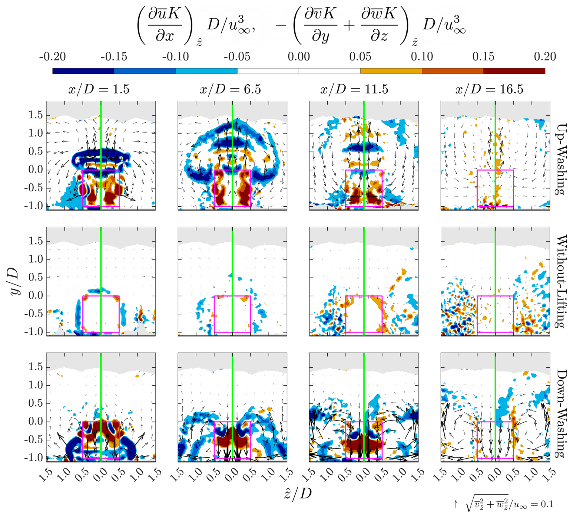
Figure 19 Contours of the terms related to energy redistribution, as defined in Eq. (7), for cases with a row spacing of 5D. The term $\partial \stackrel{\mathrm{‾}}{u}K/\partial x$ is shown on the left side of each panel, while $-(\partial \stackrel{\mathrm{‾}}{v}K/\partial y+\partial \stackrel{\mathrm{‾}}{w}K/\partial z)$ is shown on the right. Cases UW-05, WL-05, and DW-05 are displayed in the top, middle, and bottom rows, respectively. The x positions of the corresponding planes are indicated at the top of each column. Subscript $\widehat{z}$ denotes that the values of the property are averaged over the symmetry plane $z/D=\mathrm{0}$ (see Eq. 5). In-plane velocity directions are represented by arrows scaled by their magnitude, with the reference scale provided in the bottom-right corner. Note that all spatial derivatives data are filtered by averaging over a spherical volume, with the radius being 0.06D.

In Fig. 19, it is evident that the cases equipped with the lifting devices exhibit significantly positive values of 𝔸 within the MRSLs’ projection areas, indicating substantial wake recovery. In contrast, large regions with negative 𝔸 values appear outside the projection areas in cases UW-05 and DW-05, highlighting the areas from which the energy is redistributed to accelerate wake recovery. Moreover, part of the regions with negative 𝔸 appear above the top of the MRSL (y>0.0) for cases UW-05 and DW-05. This confirms that the lifting devices enhance vertical entrainment by channeling flow energy from higher altitudes downward. This effect is especially pronounced in the case with up-washing configuration, where the negative 𝔸 patches extend beyond the measurement domain after the third-row MRSL. This observation aligns well with the velocity contours shown in Fig. 13, which reveal that the wake in case UW-05 is effectively ejected into higher layers.

In contrast, compared to the cases equipped with lifting devices, regions with notable 𝔸 magnitudes are considerably smaller for case WL-05, indicating weak vertical mixing and limited energy redistribution. This pattern clearly reflects the slow wake recovery rate that conventional wind farms currently suffered.

To further investigate the mechanism of energy redistribution reflected by the term $\partial \stackrel{\mathrm{‾}}{u}K/\partial x$, Eq. (7) is utilized. This equation is derived by rearranging the transport equations of time-averaged mechanical power for incompressible flow. The terms $\partial \stackrel{\mathrm{‾}}{v}K/\partial y$ and $\partial \stackrel{\mathrm{‾}}{w}K/\partial z$ represent the spatial changing rates of mean kinetic energy due to vertical and lateral advection, respectively. Contributions from 2nd- and 3rd-order Reynolds stresses, pressure gradients, and viscous effects are collectively grouped into the residual term ℝ.

$$\begin{array}{}\text{(7)}& \begin{array}{rl}& \underset{\mathrm{SCR}\mathrm{of}\mathrm{MKE}\mathrm{flux}\mathrm{in}x\text{direction}\left(\mathbb{A}\right)}{\underbrace{{\displaystyle \frac{\partial \stackrel{\mathrm{‾}}{u}K}{\partial x}}}}=\\ & -\left(\underset{\mathrm{SCR}\mathrm{of}\mathrm{MKE}\mathrm{flux}\mathrm{in}y\text{direction}\left(\mathbb{B}\right)}{\underbrace{{\displaystyle \frac{\partial \stackrel{\mathrm{‾}}{v}K}{\partial y}}}}\right.\\ & \left.+\underset{\mathrm{SCR}\mathrm{of}\mathrm{MKE}\mathrm{flux}\mathrm{in}z\text{direction}\left(\mathbb{C}\right)}{\underbrace{{\displaystyle \frac{\partial \stackrel{\mathrm{‾}}{w}K}{\partial z}}}}\right)\\ & +\underset{\mathrm{residuals}}{\underbrace{\mathbb{R}}}\end{array}\end{array}$$

The contributions of the SCR of MKE in the y and z directions, denoted by $-(\mathbb{B}+\mathbb{C})$, are shown on the right side of each panel in Fig. 19. Comparison with the corresponding 𝔸 distributions on the left sides of the panels reveals that the residual term ℝ is generally small, especially for the cases with lifting devices. The low magnitudes of ℝ suggest that energy redistribution in the RGWFs studied is primarily governed by advection processes, such that $\mathbb{A}\simeq -(\mathbb{B}+\mathbb{C})$. This finding is consistent with previous numerical studies (Li et al., 2025b, c). Importantly, this indicates that the wake recovery mechanism in RGWFs fundamentally differs from that of conventional wind farms. While RGWFs rely mainly on advective transport to redistribute the flow energy, conventional wind farms depend more heavily on the processes driven by Reynolds stresses (Calaf et al., 2010; Porté-Agel et al., 2020). (Recall that the contributions of Reynolds stresses are accounted by the residual term ℝ.)

3.6.2 Comparing with the prior numerical predictions

This part compares the experimental results of the present study with the numerical outcomes of Li et al. (2025b), who conducted large-eddy simulation (LES) using actuator methods to investigate the wake aerodynamics of stand-alone MRSL with different configurations of lifting devices. The primary aim of this part is to demonstrate that the predictions from these prior simulations align well with the current experimental data, thereby reinforcing the credibility of the conclusions drawn based on those numerical outcomes. Furthermore, the comparison also provides some other insights – for instance, indirectly showing that the general wake aerodynamics of MRSLs is mainly governed by the thrust coefficient and the lift-to-thrust ratio.

Cases UW-10, WL-10, and DW-10 from the current experiments are compared with cases UW-17, WL-17, and DW-17 from their simulations. The suffixes refer to the row spacing and the inflow turbulence intensity used in each study, respectively. For the purpose of this comparison, the flow fields of the experimental cases with Δ_R=10D can be considered representative of stand-alone MRSL behavior for $x/D<\mathrm{9.0}$, as the MRSLs in the second row have a negligible to limited influence. Note that N in Eq. (5) is set to 1 everywhere when treating the simulation data.

The numerical setup in Li et al. (2025b) is broadly comparable to the present experiments. In particular, the ground clearance of MRSL is 0.10D, the thrust coefficient C_T for the configuration without lifting devices is 0.71, the normalized lift force ${\widehat{L}}^{\mathrm{W}}$ (see Eq. 1) is approximately 100 %, the inflow is without vertical velocity shear, and the inflow turbulence intensity is 1.74 %. However, key differences exist. Their simulations use full-scale MRSLs with a side length of D=300 m and a freestream velocity of u_∞=10.1 m s⁻¹, resulting in a Reynolds number $R{e}_{\mathrm{D}}\stackrel{\Delta }{=}{u}_{\mathrm{\infty }}D/\mathit{\nu }$ of approximately 2.0×10⁸. In contrast, the Reynolds number in the current experiments is around 1.4×10⁵, giving a significant mismatch. Additionally, the simulated MRSLs in Li et al. (2025b) are equipped with four wings rather than three, and the floor boundary conditions are modeled as a slip wall, unlike the physical floor present in the experiments. For further details on their numerical setup, readers are referred to Li et al. (2025b).

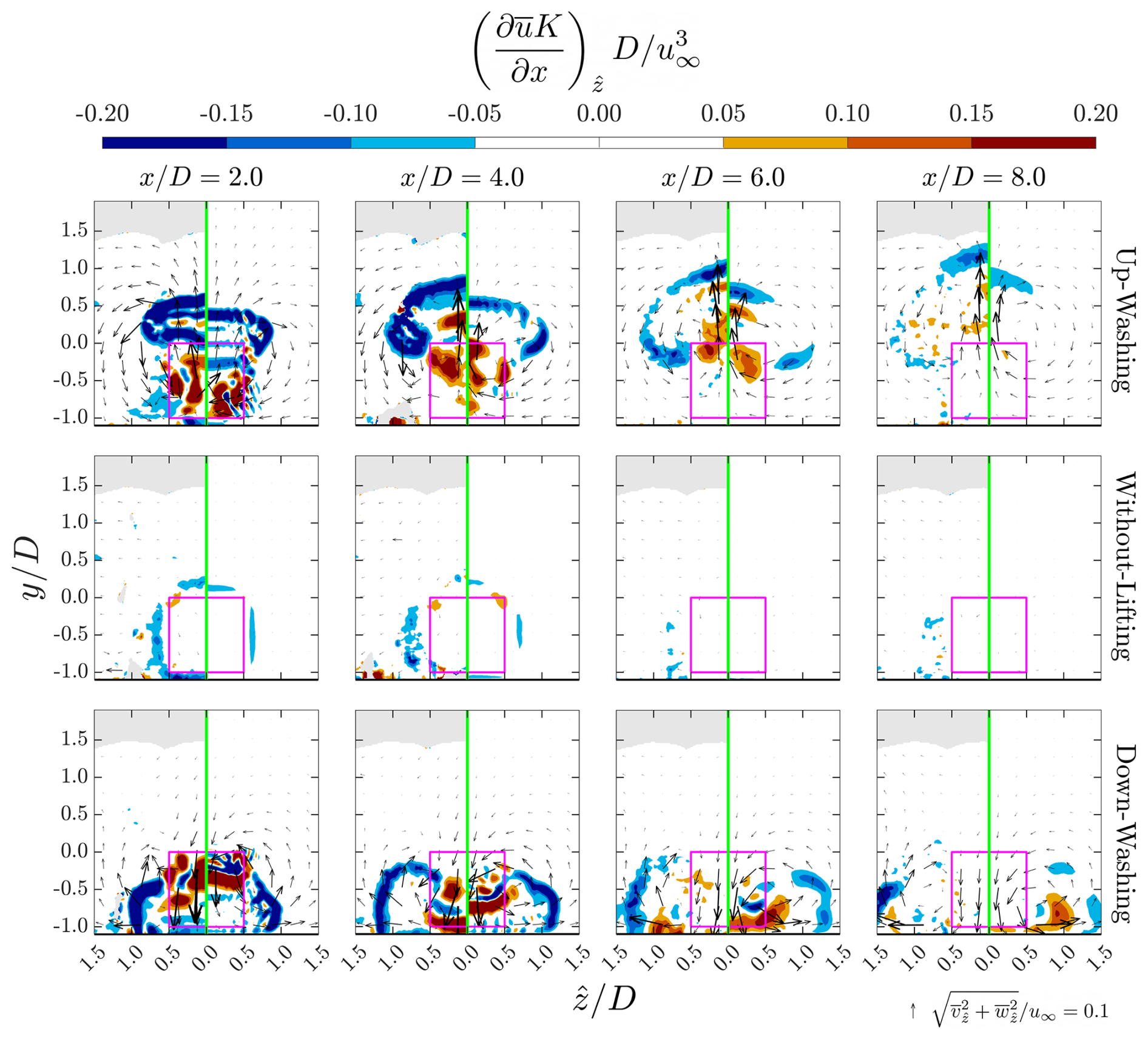
Figure 20 Contours of $\partial \stackrel{\mathrm{‾}}{u}K/\partial x$, as defined in Eq. (7), for cases with a row spacing of 10D (UW-10, WL-10, and DW-10), along with the corresponding numerical results from Li et al. (2025b). See the main text for the key parameters of their numerical setup. In each panel, experimental results are shown on the left, and LES results from Li et al. (2025b) are shown on the right. The up-washing, without-lifting, and down-washing configurations are displayed in the top, middle, and bottom rows, respectively. The x positions of the corresponding planes are indicated at the top of each column. Subscript $\widehat{z}$ denotes that the values of the property are averaged over the symmetry plane $z/D=\mathrm{0}$ (see Eq. 5). In-plane velocity directions are represented by arrows scaled by their magnitude, with the reference scale provided in the bottom-right corner. Note that all spatial derivatives data from the experiments are filtered by averaging over a spherical volume, with the radius being 0.06D.

Figure 20 presents contour plots of $\partial \stackrel{\mathrm{‾}}{u}K/\partial x$ from both the current experiments and the LES results reported by Li et al. (2025b). In each panel, the experimental data are shown on the left, and the corresponding LES predictions are shown on the right. Overall, the experimental and numerical results show strong agreement across all three configurations, despite the significant discrepancies in the Reynolds number Re_D and some differences in experimental setup and numerical modeling. Both datasets consistently demonstrate that the up-washing and down-washing configurations exhibit substantially stronger wake recovery compared to the configuration without lifting devices. In particular, for the up-washing configuration, both results indicate that wake recovery is primarily driven by the redistribution of flow energy from upper to lower layers.

The strong agreements described above demonstrate cross-validation between the present experimental data and prior LES predictions, showing that independent methodologies yield consistent outcomes and lead to the same conclusions. Besides, these agreements also provide preliminary insight into the dominant parameters governing MRSL wake aerodynamics. In particular, the results suggest that the thrust coefficient and lift-to-thrust ratio may be key drivers. This hypothesis is supported by the fact that the two datasets, despite differing substantially in configuration (e.g., absolute scale, number of wings, and wing placement), reveal consistent aerodynamic trends. Nevertheless, this remains an initial hypothesis. Future studies are required to systematically test this idea, as identifying the dominant aerodynamic parameters would provide a crucial foundation for developing analytical models and engineering tools for RGWF design and optimization.

On the other hand, although the current experimental results align well with the numerical findings of Li et al. (2025b), several subtle differences are observed. Notably, in the experiments, wake development appears to occur more rapidly in the cases with lifting devices compared to the simulations. This discrepancy is likely due to the distribution of lift forces (L^W) being more concentrated on the top wing of the MRSL in the experiments. In the experimental setup, the top wing is exposed to undisturbed flow, while the lower wings operate within the wake of the porous disk, resulting in reduced lift (see Appendix B2). In contrast, the numerical simulations model all wings as overlapping with the actuator disk, leading to a more uniform distribution of lift among them. This difference likely causes the MRSLs in the experiments to generate circulation systems concentrated at higher vertical positions, and this may explain why the experimental wakes develop faster than those observed in the simulations. These observations not only highlight the discrepancies between the datasets but also may provide insight for future MRSL optimization, such as fine-tuning wing placement and pitch settings to achieve a more effective distribution of lift across the MRSL's height.

3.7 RGWF with the staggered layout

This section addresses the aerodynamics of RGWFs when MRSLs in different rows are not aligned with the streamwise direction. Understanding this aspect is essential for bringing RGWF from concept to practical application. In real-world scenarios, while prevailing wind directions may exist, wind directions at wind farm sites vary over time. As a result, if MRSLs always face against the inflow direction, the effective layout of an RGWF continuously changes. Previous studies have shown that wind farm layout significantly influences the power output of conventional wind farms (Barthelmie et al., 2010; Stevens et al., 2016). For RGWFs, layout sensitivity is postulated to be even more pronounced. This expectation is supported by the discussion in Sect. 3.4, which highlights the fact that enhanced vertical energy entrainment in RGWFs originates from streamwise vortical structures that accumulate strength progressively when MRSLs are arranged in a streamwise-aligned layout.

To preliminarily assess whether the effectiveness of RGWF is sensitive to wind farm layout, a case with a staggered wind farm layout is tested, which is case UW-05-ST listed in Table 1. The case features two rows of MRSLs that are not aligned with the inflow direction. The detailed dimensions of the RGWF layout for this case have been given in Sect. 2.3.

3.7.1 Contours of the time-averaged streamwise velocity, streamwise vorticity, and lateral velocity

Figures 21 to 23 present the contours of time-averaged streamwise velocity $\stackrel{\mathrm{‾}}{u}$, time-averaged streamwise vorticity ${\stackrel{\mathrm{‾}}{\mathit{\omega }}}_x$, and time-averaged vertical velocity $\stackrel{\mathrm{‾}}{v}$ at several x planes for the case with staggered wind farm layout. The in-plane velocity components $\stackrel{\mathrm{‾}}{v}$ and $\stackrel{\mathrm{‾}}{w}$ are superimposed as arrows to illustrate the flow direction. For comparison, results from the aligned up-washing case UW-05 are also shown alongside. However, it should be noted that at $x/D=\mathrm{10.4}$, direct comparison becomes less meaningful, as case UW-05 includes third-row MRSLs, whereas case UW-05-ST does not.

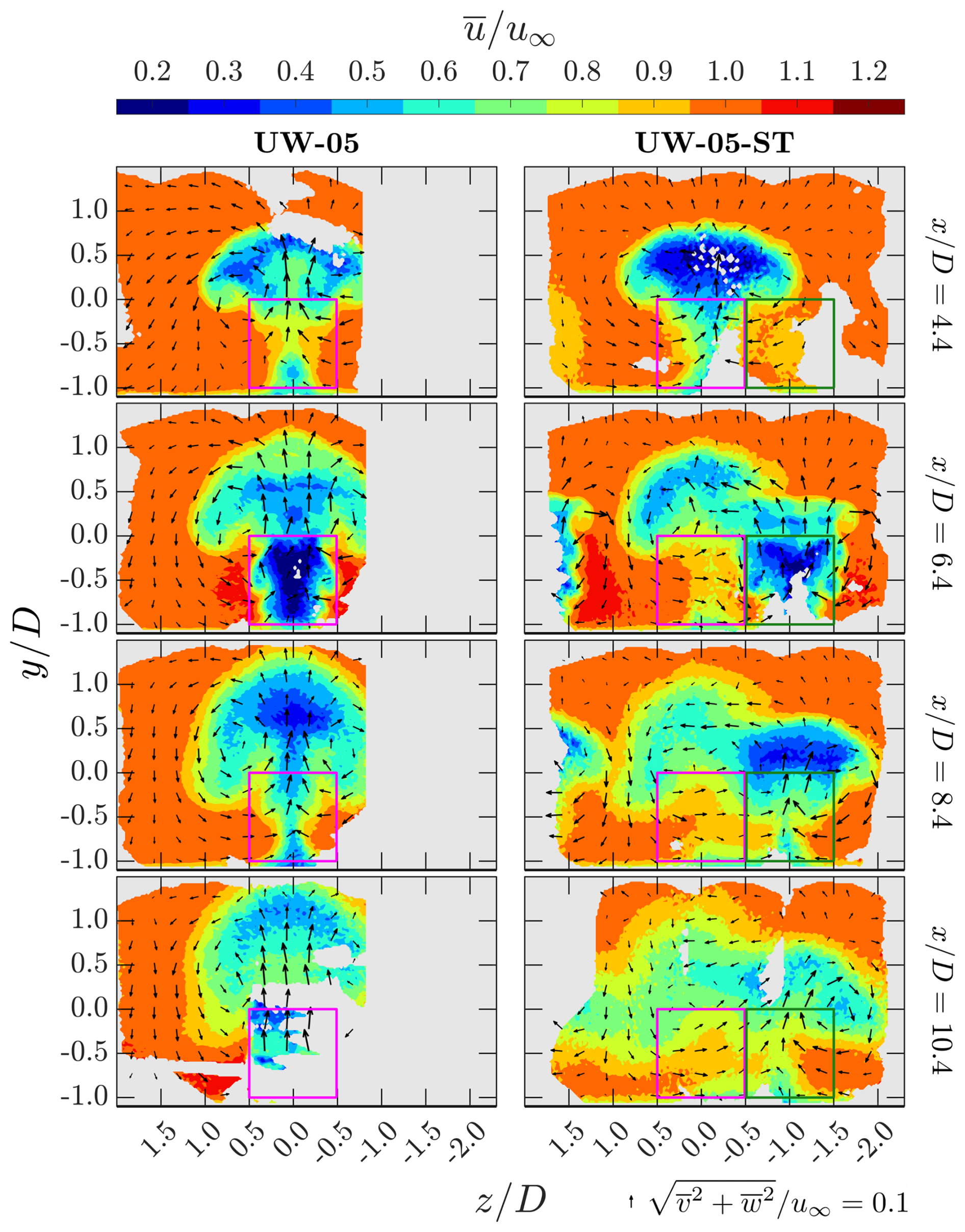
Figure 21 Contours of the time-averaged streamwise velocity $\stackrel{\mathrm{‾}}{u}$ at selected x planes for the two up-washing cases. The case with the aligned layout (case UW-05) and the staggered layout (case UW-05-ST) are presented in the left and right column, respectively. The corresponding x positions are indicated on the right side of each row. For the aligned case, MRSL projection areas are marked with magenta squares. For the staggered case, the projection areas of the first- and second-row MRSLs (see Fig. 7) are shown in magenta and dark-green squares, respectively. In-plane velocity directions are represented by arrows scaled by their magnitude, with the reference scale provided at the bottom-right corner of the figure.

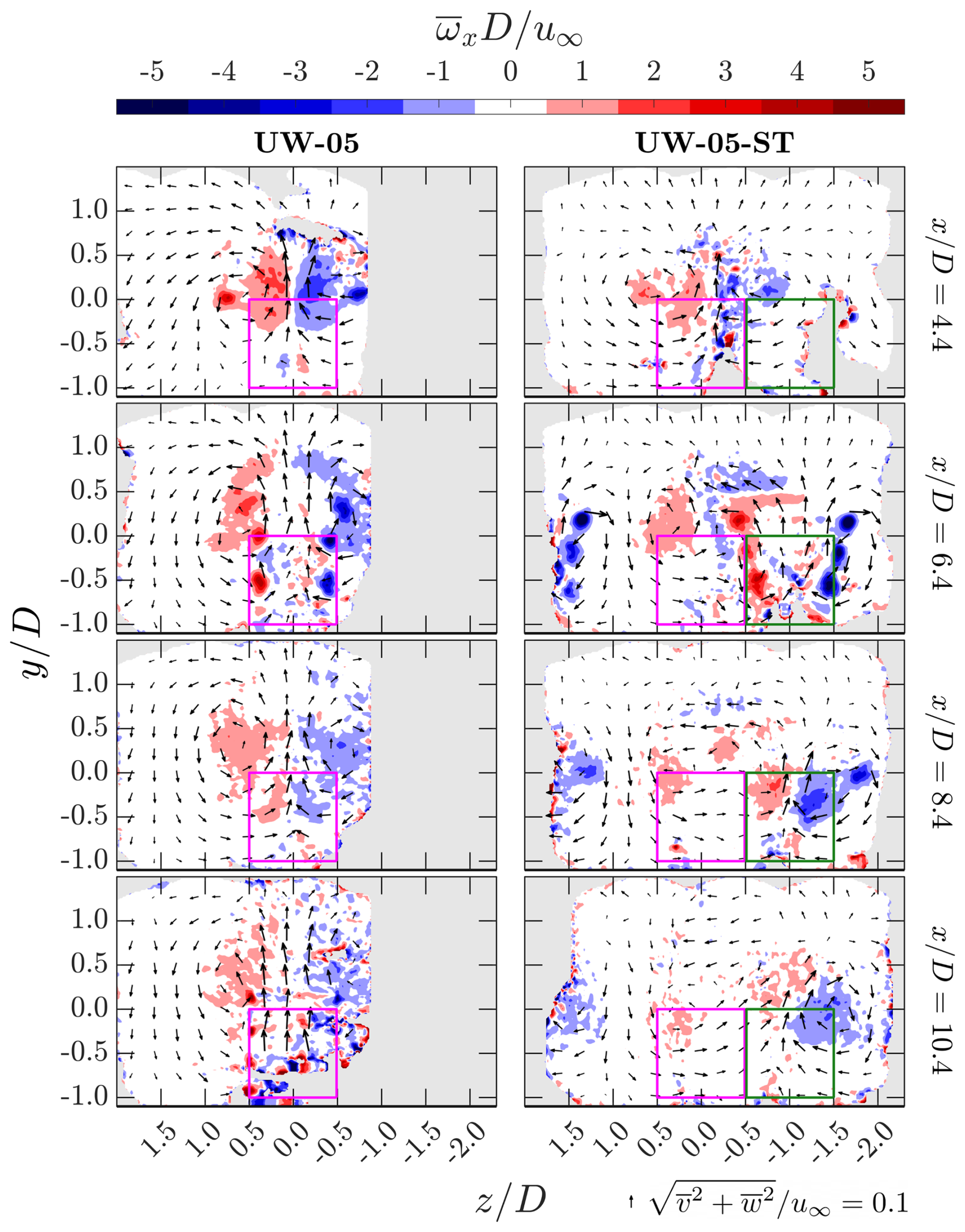
Figure 22 Contours of the time-averaged streamwise vorticity ${\stackrel{\mathrm{‾}}{\mathit{\omega }}}_x$ at selected x planes for the two up-washing cases. The case with the aligned layout (case UW-05) and the staggered layout (case UW-05-ST) are presented in the left and right column, respectively. The corresponding x positions are indicated on the right side of each row. For the aligned case, MRSL projection areas are marked with magenta squares. For the staggered case, the projection areas of the first- and second-row MRSLs (see Fig. 7) are shown in magenta and dark-green squares, respectively. In-plane velocity directions are represented by arrows scaled by their magnitude, with the reference scale provided at the bottom-right corner of the figure.

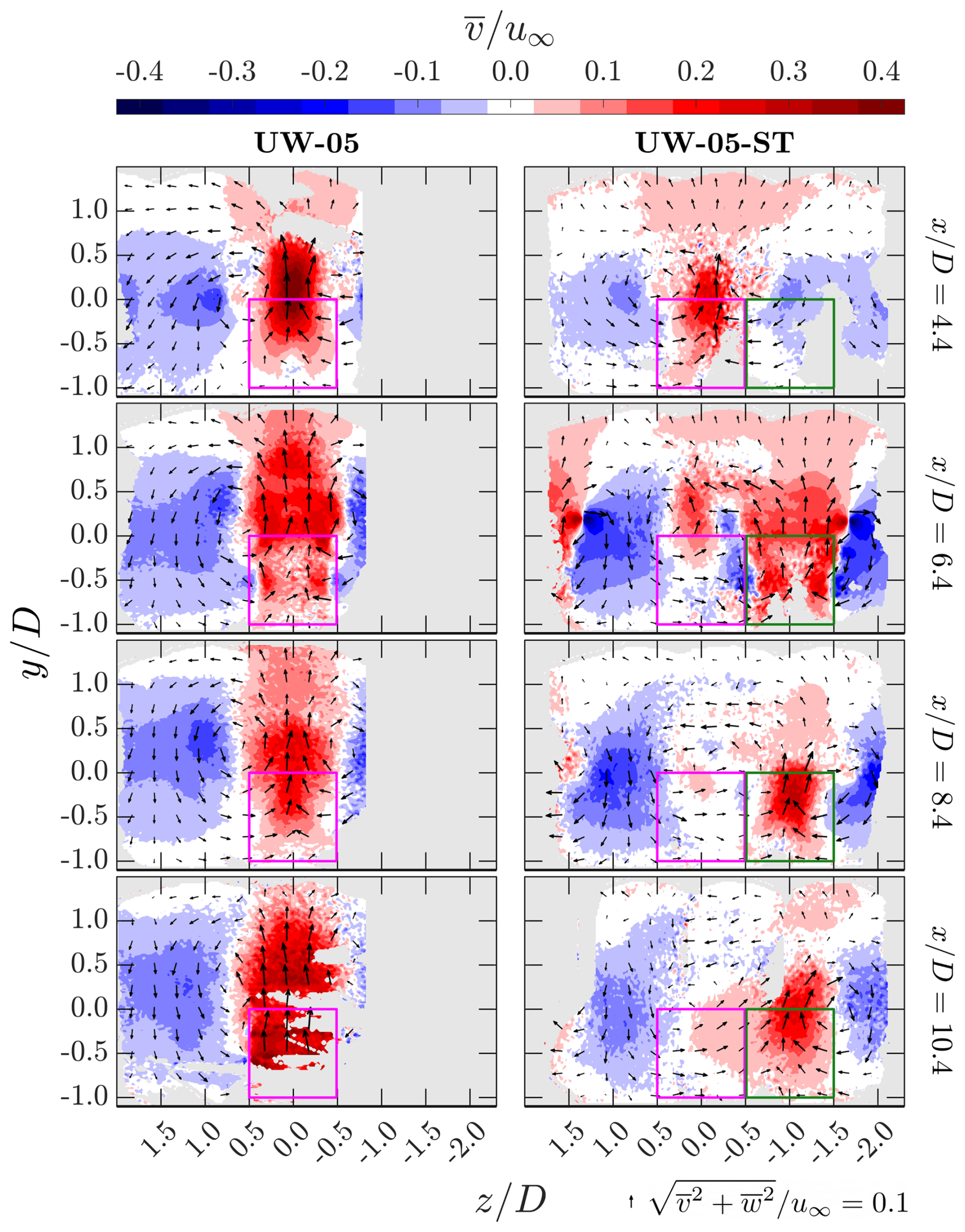
Figure 23 Contours of the time-averaged vertical velocity $\stackrel{\mathrm{‾}}{v}$ at selected x planes for the two up-washing cases. The case with the aligned layout (case UW-05) and the staggered layout (case UW-05-ST) are presented in the left and right column, respectively. The corresponding x positions are indicated on the right side of each row. For the aligned case, MRSL projection areas are marked with magenta squares. For the staggered case, the projection areas of the first- and second-row MRSLs (see Fig. 7) are shown in magenta and dark-green squares, respectively. In-plane velocity directions are represented by arrows scaled by their magnitude, with the reference scale provided at the bottom-right corner of the figure.

As expected, at $x/D=\mathrm{4.4}$, which is the plane located just upstream of the second-row MRSLs, the contours of $\stackrel{\mathrm{‾}}{u}$, ${\stackrel{\mathrm{‾}}{\mathit{\omega }}}_x$, and $\stackrel{\mathrm{‾}}{v}$ are generally similar between cases UW-05 and UW-05-ST. Minor differences may be attributed to the variations introduced while manually reassembling RGWFs.

At $x/D=\mathrm{6.4}$ and 8.4, which are both downstream of the second-row MRSLs, the effects of staggering become pronounced. In case UW-05-ST, Fig. 21 shows that the wake of the second-row center-column MRSL is centered around $z/D=-\mathrm{1.0}$, and the wake of the side-column MRSL located on the positive z side is also visible. Examining the swirling motions depicted by the in-plane velocity vectors, the counter-rotating vortex pair in the staggered case appears asymmetric. Specifically, the vortex on the negative z side is smaller in size, while the one on the positive z side is larger. Although the vortex shapes are altered by the misalignment, the updraft and downdraft motions found in case UW-05-ST remain significantly stronger than those in the without-lifting case, as evident from the in-plane velocity arrows in Fig. 17. This suggests that the vertical entrainment remains robust in the staggered-up-washing case and is still substantially stronger than that in the without-lifting case.

Examining the contours of ${\stackrel{\mathrm{‾}}{\mathit{\omega }}}_x$ for case UW-05-ST at $x/D=\mathrm{6.4}$ and 8.4 in Fig. 22, it is evident that vortical structures generated by the first-row center-column MRSL and the second-row side-column MRSL jointly contribute to downdraft motions at around $z/D=\mathrm{1.0}$. This observation indicates that the interaction between vortical structures released by adjacent columns is increased with the staggered RGWF layout. Moreover, the vorticity contours show that positive ${\stackrel{\mathrm{‾}}{\mathit{\omega }}}_x$ generated by the second-row center-column MRSL overlaps with negative ${\stackrel{\mathrm{‾}}{\mathit{\omega }}}_x$ originating from the first-row center-column MRSL. These interactions reduce the strength of the positive ${\stackrel{\mathrm{‾}}{\mathit{\omega }}}_x$, ultimately causing the in-plane velocity field to skew toward the negative z direction. Despite this attenuation of vorticity, the vertical flow induced by the lifting devices remains strong in case UW-05-ST, indicating that vertical entrainment continues to be significantly enhanced.

Although the contours of $\stackrel{\mathrm{‾}}{u}$ and ${\stackrel{\mathrm{‾}}{\mathit{\omega }}}_x$ suggest that the RGWF concept is not significantly weakened by the misalignment, the time-averaged vertical velocity $\stackrel{\mathrm{‾}}{v}$ contours in Fig. 23 indicate that vertical flows are somewhat less intense in the staggered layout compared to the aligned one. This conclusion is drawn from the $\stackrel{\mathrm{‾}}{v}$ fields at $x/D=\mathrm{6.4}$ and 8.4, which show that regions of strong vertical velocity penetrate to higher altitudes in case UW-05 than in case UW-05-ST. Specifically, regions with $\stackrel{\mathrm{‾}}{v}/u_{\mathrm{\infty }}>\mathrm{0.1}$ can only be found below $y/D=\mathrm{0.5}$ for case UW-05-ST, while those regions can be found above $y/D=\mathrm{1.2}$ for case UW-05. This indicates that, in the staggered case, a thinner upper-layer flow contributes to wake re-energization, whereas the aligned configuration draws energy from a thicker vertical region. The maximum altitude from which RGWF can entrain energy is considered critical, as it is believed to directly influence the power performance of large-scale RGWFs. Nevertheless, even at $x/D=\mathrm{10.4}$, which is more than 5D downstream from the nearest MRSL, case UW-05-ST still exhibits vertical flows that are stronger than 0.1u_∞ at 0.3D above the top of the MRSL. This observation preliminarily confirms that the MRSL concept remains effective, even under the tested staggered layout.

3.7.2 Area-averaged available power

To provide a more quantitative assessment of the effectiveness of RGWFs under the staggered layout, the area-averaged available power $<{\stackrel{\mathrm{‾}}{u}}_{\widehat{z}}^{\mathrm{3}}{>}_{\widehat{z}\in [a,b]}$, as defined in Eq. (6), is examined. Specifically, $<{\stackrel{\mathrm{‾}}{u}}_{\widehat{z}}^{\mathrm{3}}{>}_{\widehat{z}\in [a,b]}$ is evaluated for cases UW-ST-05 and UW-05 using two ranges of [a,b], namely $[-\mathrm{0.5}D,\mathrm{0.5}D]$ and $[-\mathrm{1.5}D,-\mathrm{0.5}D]$, and the results are shown in Fig. 24. These two intervals correspond to the areas enclosed by the magenta and dark-green squares in Figs. 21 to 23, and are hereafter referred to as the plus-side and minus-side for convenience, with the namings based on their lateral coordinates.

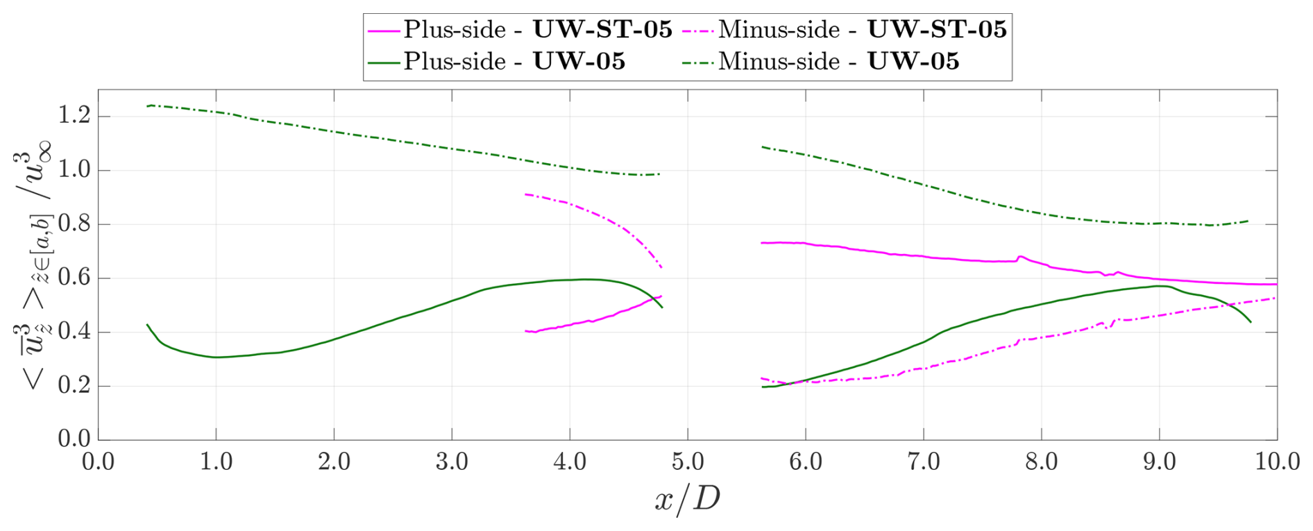
Figure 24 Area-averaged available power for cases UW-ST-05 and UW-05. The plus-side (solid lines) correspond to $<{\stackrel{\mathrm{‾}}{u}}_{\widehat{z}}^{\mathrm{3}}{>}_{\widehat{z}\in [a,b]}$ calculated with [a,b] being $[-\mathrm{0.5}D,\mathrm{0.5}D]$ and the minus-side (dashed lines) is calculated with [a,b] being $[-\mathrm{1.5}D,-\mathrm{0.5}D]$. Note that mirror averaging is not applied for case UW-ST-05 as $z/D=\mathrm{0.0}$ is no longer the mirror plane. In short, $\widehat{z}$ is replaced with z when calculating $<{\stackrel{\mathrm{‾}}{u}}_{\widehat{z}}^{\mathrm{3}}{>}_{\widehat{z}\in [a,b]}$ for case UW-ST-05. The definition of $<{\stackrel{\mathrm{‾}}{u}}_{\widehat{z}}^{\mathrm{3}}{>}_{\widehat{z}\in [a,b]}$ is given in Eq. (6).

It should be noted that mirror averaging is not applied to case UW-05-ST, since $z/D=\mathrm{0}$ is no longer the symmetry plane. Accordingly, for $<{\stackrel{\mathrm{‾}}{u}}_{\widehat{z}}^{\mathrm{3}}{>}_{\widehat{z}\in [a,b]}$ of case UW-05-ST, all $\widehat{z}$ are replaced with z – that is, $<{\stackrel{\mathrm{‾}}{u}}_z^{\mathrm{3}}{>}_{z\in [a,b]}$. This makes the results more sensitive to the effects of unavailable data points, which occupy a relatively large portion of the dataset, as shown in Figs. 21 to 23.

Starting from comparing the results of $<{\stackrel{\mathrm{‾}}{u}}_{\widehat{z}}^{\mathrm{3}}{>}_{\widehat{z}\in [a,b]}$ between cases UW-ST-05 and UW-05, it is shown that the two curves for area-averaged available power has already diverged at $x/D=\mathrm{3.5}$. Ideally, the curves of UW-ST-05 should collapse onto those of UW-05 before being influenced by the second-row MRSLs. However, the staggered case exhibits values lower than the aligned case by approximately $\mathrm{0.16}{u}_{\mathrm{\infty }}^{\mathrm{3}}$. This deviation may be attributed to the fact the data of the two cases are collected in different measurement sessions (see Sect. 2.8) or to the greater influence of unavailable data points in the staggered configuration, since mirror-averaging cannot be applied.

Despite the data imperfections noted above, the key finding from Fig. 24 is that the minus-side of the area-averaged available power for case UW-ST-05 increases steadily over the range $\mathrm{5}<x/D<\mathrm{10}$. This trend indicates that the vortical structures remain effective in channeling the wake upward and enhancing vertical mixing, thereby confirming that the RGWF concept retains its effectiveness under the staggered layout. However, closer examination of the slopes within $\mathrm{5}<x/D<\mathrm{10}$ reveals that the plus-side of UW-05 is steeper than the minus-side of UW-ST-05, suggesting weaker wake re-energization directly downstream of the second-row MRSL projection area when the layout is changed from aligned to staggered. Nonetheless, this interpretation should be approached with caution, as the discrepancies in $<{\stackrel{\mathrm{‾}}{u}}_{\widehat{z}}^{\mathrm{3}}{>}_{\widehat{z}\in [a,b]}$ between cases UW-ST-05 and UW-05 appear to be relatively large before reaching the second-row MRSLs, as discussed in the previous paragraph.

Looking more closely at Fig. 24, it is found that the minus-side available power for case UW-05 decreases from about $\mathrm{1.2}{u}_{\mathrm{\infty }}^{\mathrm{3}}$ to $\mathrm{1.0}{u}_{\mathrm{\infty }}^{\mathrm{3}}$ in the range $\mathrm{0}<x/D<\mathrm{5}$. The fact that $<{\stackrel{\mathrm{‾}}{u}}_{\widehat{z}}^{\mathrm{3}}{>}_{\widehat{z}\in [a,b]}$ exceeds $\mathrm{1.0}{u}_{\mathrm{\infty }}^{\mathrm{3}}$ can be attributed to the blockage effect of the first-row MRSLs. Note that as this high-velocity flow is directed into the plus-side region by the streamwise vortical structures, replenishment occurs mainly from above (i.e., $y/D>\mathrm{0}$), where the velocity is approximately 1.0u_∞. This mechanism largely explains the observed drop on this curve. The same reasoning also applies to the minus-side of UW-ST-05 in $\mathrm{0}<x/D<\mathrm{5}$, as well as to the minus-side of UW-05 in $\mathrm{5}<x/D<\mathrm{10}$.

For the plus-side of UW-ST-05 in $\mathrm{5}<x/D<\mathrm{10}$, the analysis is less straightforward due to strong influence from the wake aerodynamics of the first-row MRSL. Nevertheless, the results suggest that the wake that has been ejected over the MRSL’s top is not substantially brought back down into the plus-side region by the vortical structures. This interpretation is supported by the fact that $<{\stackrel{\mathrm{‾}}{u}}_{\widehat{z}}^{\mathrm{3}}{>}_{\widehat{z}\in [-\mathrm{0.5}D,\mathrm{0.5}D]}$ for UW-ST-05 does not drop sharply. Figure 21 also shows that the low-velocity wake largely remains above $y/D=\mathrm{0}$ within $-\mathrm{0.5}<z/D<\mathrm{0.5}$.

It should be noted, however, that the present setup only considers two rows of MRSLs. As more rows are added, wake recycling may happen, a trend already hinted at by the $\stackrel{\mathrm{‾}}{u}$ contours at $x/D=\mathrm{10.4}$ for UW-ST-05 in Fig. 21.

3.7.3 Remarks for the staggered case

The results presented in this part provide preliminary evidence that the RGWF concept remains effective under a staggered layout, supporting its robustness. However, the current study investigates only a single scenario with two rows of MRSLs. Further investigations across a wider range of RGWF layouts, including additional rows and alternative arrangements, are needed to establish a more comprehensive understanding. Such insight is particularly important for accurately estimating annual energy production (AEP) of RGWFs, given that wind direction can vary across the full 360°, resulting in a wide range of effective wind farm layouts. Reliable AEP prediction is critical for advancing RGWFs from concept to commercial deployment, as it directly influences the calculation of the levelized cost of energy (LCoE), which is a key metric in assessing economic viability. Ultimately, financial feasibility remains one of the most dominant factors driving the development of renewable energy technologies (Lazard, 2024; McCoy et al., 2024).

4 Conclusions

This study experimentally investigated the aerodynamic performance of regenerative wind farms (RGWFs), a newly proposed wind farm concept. Unlike conventional wind farms that use typical single-rotor horizontal-axis wind turbines, RGWFs are composed of multi-rotor systems with lifting devices (MRSLs). These machines were specifically engineered to achieve faster wake recovery rates compared to traditional wind turbines, and this is realized through incorporating the lifting devices that are dedicated to inducing large-scale streamwise vortical structures (see Fig. 1). The current results demonstrated that these vortical structures significantly enhanced vertical energy entrainment within RGWFs, substantially accelerating the wake recovery and improving the wind farm performance. In particular, when the MRSLs of an entire RGWF are equipped with the lifting devices, the thrust readings of the second-row MRSLs are more than three times than those without.

In addition to experimentally demonstrating the potential of RGWFs, the results of this study preliminarily indicated that RGWFs perform well whether adjacent rows are aligned or staggered with the streamwise direction, reinforcing the robustness of the concept. Moreover, the current experimental findings showed strong agreement with previous numerical simulations (Li et al., 2025b, c), both showing that the wake recovery rates were accelerated due to the enhanced vertical energy entrainment driven by the vortical structures induced by the lifting devices. This cross-validation between simulations and experiments reinforces the credibility of the RGWF concept and provides a solid foundation for following research.

Despite the encouraging outcomes, several areas are recommended for further investigation. First, the current study focused on a limited set of layouts and examined only the up-washing configuration for the staggered layout. Future work should explore broader ranges of RGWF layouts, including various misalignment patterns, to fully characterize system performance at more realistic wind farm sites. Second, instead of using uniform inflow profiles with low turbulence levels, which is unrealistic out in the field, future studies should incorporate inflow conditions that more closely resemble atmospheric boundary layers. Currently, the effects of vertical velocity shear, turbulence intensity, and thermal stability of the incoming flow on RGWF's performance remain largely underexplored and warrant systematic investigations. Third, optimizing the MRSL design is critical. This involves evaluating the relative advantages and disadvantages of up-washing versus down-washing configurations, as well as determining the optimal wing geometry (airfoil type, chord, span, and twist), number of wings, and wing placement. Fourth, the detailed aerodynamics of a realistic MRSL requires further investigation. In particular, replacing the porous disks used in this study with rotating machines would enable an assessment of whether the overall wake behavior is influenced by aerodynamic interactions between the wakes of rotating blades and the wings. Lastly, since the effectiveness of RGWF has been validated through both simulations and wind tunnel experiments, the next straightforward step is to test an MRSL prototype under natural wind conditions. This test would not only validate the practicality of the concept but would also provide valuable information on structural robustness, control system integration, and long-term energy yield in real-world environments.

In summary, the experimental results validate the aerodynamic advantages of RGWFs, demonstrating that this novel wind farm concept can substantially outperform the conventional counterpart in terms of wake recovery and land efficiency. However, further research is required to advance RGWFs from a promising conceptual framework to a practical and cost-effective solution for harvesting renewable energy on a large scale.

Appendix A: Detail descriptions of the particle tracking velocimetry system

A detailed description of the setup for the three-dimensional particle tracking velocimetry (3D-PTV) used in this work is provided in this appendix. The specifications of the software and hardware utilized are outlined in the following.

• Software. Commercial software packages DaVis 10 (by LaVision GmbH) are used for image acquisition and detecting the tracer particles.

• Seeding of the tracer particles. Neutrally buoyant helium-filled soap bubbles (HFSBs) with a median diameter of approximately 300 to 400 µm (Scarano et al., 2015; Faleiros et al., 2019) are used as flow tracers. The HFSBs are released from an in-house developed seeding system located in the settling chamber of the wind tunnel. This system is reported to have a minimal impact on the flow. In particular, the turbulence intensity is increased by approximately 0.5 % to 0.8 % (Giaquinta, 2018). The seeding system measures approximately 1000 mm in the lateral direction and 2000 mm in the vertical direction. However, due to the contraction at the wind tunnel exit, the lateral width of the seeded region narrows to about 570 mm as the tracers reach the region of interest. The seeding system can be slid laterally to accommodate different measurement volumes. For more detailed specifications of the seeding system, refer to Terra et al. (2024) and Bensason et al. (2025).

• Illuminating source. The tracer particles are illuminated using two LED arrays that emit blue light (LED-Flashlight 300 blue, LaVision GmbH). Each array has a dimension approximately 330 mm by 110 mm. During the measurements, the LED arrays are positioned beneath the wind farm by around 1200 mm and aligned in the streamwise direction, with their longer sides parallel to the flow. The entire FOV is observed to be adequately illuminated after the light sheet expands (see Fig. 3).

• Cameras and field of view. Three high-speed cameras (Photron Mini AX100) are used, each equipped with a CMOS image sensor of 1024 px × 1024 px and a uniform pixel pitch of 20 µm. As shown in Fig. 3, the three cameras are mounted on a straight column aligned with the vertical direction (y direction), with separations of approximately 700 mm. The bottom-most camera is positioned at a height around the center of the MRSL, and the maximum angle of the cameras is about 36°. The lateral distance (z direction) between the cameras and the center of the FOV is approximately 2150 mm. The focal lengths of the objective lenses are 50, 50, and 60 mm for the bottom, middle, and top cameras, respectively. An f# of 16 is used, providing a depth of focus of around 1000 mm. The FOV for this setup measures 830, 550, and 880 mm in the streamwise, lateral, and vertical directions, corresponding to 2.8D,1.8D, and 2.9D, respectively. Note that the lateral thickness of the FOV is limited by the seeding of the tracer particles. The center of the FOV is located near the top of the MRSL, and the scaling factor for this setup is approximately 0.85 mm px⁻¹.

• Traverse system. The cameras and the illumination system are mounted on a traverse system (see Fig. 3), enabling quick shifts of the measurement volume. The traverse system has a range of 1500 mm in the streamwise direction and 1000 mm in the lateral direction. Its precision is 1 mm. The traverse system step size in streamwise and lateral directions (Δ_Tra,x and Δ_Tra,z) are set to 600 and 375 mm, respectively. During the measurement campaign, the traverse system is manually repositioned to cover the entire region of interest, as described in Sect. 2.8 and illustrated in Fig. 6. Note that larger overlapping regions between FOVs are used when the traverse system is manually repositioned.

• Camera calibration. The initial geometric calibration of the cameras is performed by fitting a 3rd-order polynomial to an image of a calibration plate. Subsequently, a volume self-calibration is applied by taking images of flow field, reducing the root mean square of image distortion residuals to less than 0.1 voxels. The geometric calibration is repeated at the beginning of each day and whenever the traverse system is repositioned manually, while the volume self-calibration is frequently re-applied to maintain the quality of the calibration.

Appendix B: Preliminary tests for designing the MRSL model

This appendix summarizes the parameter selection process for the MRSL's aerodynamic model described in the main text, with the model consisting of a porous disk with wings attached. The selection process is based on the preliminary wind tunnel tests. The primary objectives of these tests are to find an appropriate airfoil profile for the MRSL’s lifting devices, determine suitable pitch angles for the wings, and provide benchmark data to guide the final design of the MRSL's model.

The preliminary tests were conducted in a low-speed wind tunnel (W-Tunnel) at the aerodynamic laboratories of the Delft University of Technology prior to the main experimental campaign. The wind tunnel operates as an open jet with an exit cross-section of 600×600 mm². Photos of the experimental setup are shown in Fig. B1. It should be noted that the floor is not included in these preliminary tests. The coordinate axes x, y, and z correspond to the (equivalent) streamwise, vertical, and lateral directions as those in the main context.

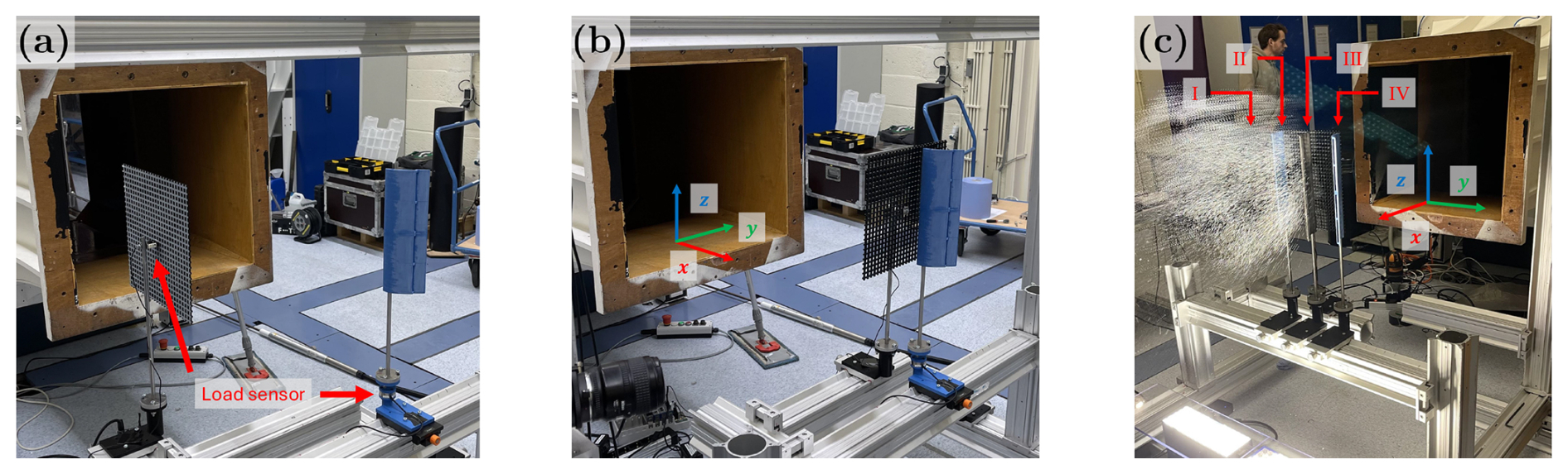
Figure B1 (a) Experimental setup for the preliminary tests to evaluate wing performance. The load sensors for both the wing and the porous disk are indicated by red arrows (the porous disk in this photo is positioned outside the jet). (b) Setup for evaluating the combined performance of the single wing and the disk. (c) Photograph showing the positions of the loci for the wings. The configuration shown represents the Up-Washing configuration, with the wing at locus I absent. This photo was taken during the 3D-PTV measurements.

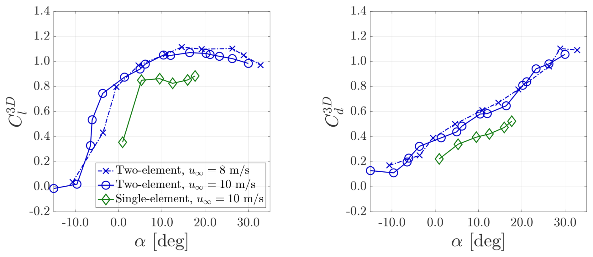
Figure B2 Time-averaged three-dimensional lift coefficients ($C_{\mathrm{l}}^{\mathrm{3}\mathrm{D}}$) and drag coefficients ($C_{\mathrm{d}}^{\mathrm{3}\mathrm{D}}$) measured in the preliminary experimental tests. The profiles of the tested airfoils are shown in Fig. B3, and the experimental setup is depicted in Fig. B1. The resolutions of the load sensor are below $\mathrm{0.01}{C}_{\mathrm{l}}^{\mathrm{3}\mathrm{D}}$ and $\mathrm{0.01}{C}_{\mathrm{d}}^{\mathrm{3}\mathrm{D}}$, while the uncertainties of the angle of attack α are approximately 1°.

B1 Evaluation of the multi-element airfoil

This part benchmarks the performance of the MRSL’s wings used in the final design, and their airfoil profile is categorized as multi-element airfoils. While single-element airfoils are simpler, multi-element airfoils may be preferred as they tend to offer higher maximum lift coefficients (C_l,max) (Smith, 1975). For this reason, a two-element airfoil designed by Broertjes (2024) is selected as the candidate for the MRSL's model. The configuration consists of two E423 airfoils (Selig et al., 1997) and is optimized using the MSES software (Drela, 2015). The profile of the selected two-element airfoil is shown on the left side of Fig. B3. Although multi-element airfoils that offer even higher C_l,max exist, this particular profile is chosen for its relatively simple structure (facilitating manufacturing), high thickness-to-chord ratio (aiding assembly and installation), and moderate camber (reducing flow blockage). Additionally, for comparison, a single-element S1223 airfoil (shown on the right of Fig. B3) (Selig et al., 1995) is also tested to verify whether the selected two-element airfoil provides superior lift performance.

For the tested wings, the span and chord are set to 300 and 100 mm, respectively, matching the dimensions of the final MRSL design. Their performance is evaluated using three-dimensional lift and drag coefficients ($C_{\mathrm{l}}^{\mathrm{3}\mathrm{D}}$ and $C_{\mathrm{d}}^{\mathrm{3}\mathrm{D}}$). The forces are measured using a six-axis force-torque sensor (F/T Sensor: mini40 with SI-40-2 calibration, ATI Industrial Automation), with a precision of 0.01 N. The sampling rate is set to 500 Hz, and the measurements are conducted over a duration of 20 s. The wings and sensors are mounted on a frame using a combination of metallic (LINOS X95 System) and 3D-printed components, as shown in Fig. B1.

$C_{\mathrm{l}}^{\mathrm{3}\mathrm{D}}$ and $C_{\mathrm{d}}^{\mathrm{3}\mathrm{D}}$ for the wings with the two airfoil profiles are plotted as functions of the angle of attack α in Fig. B2. The tests are conducted at reference velocities of 8 and 10 m s⁻¹ for the wings with the two-element airfoil and at 10 m s⁻¹ for those with the single-element airfoil. Angles of attack are measured before and after testing using a camera and image processing software (ImageJ, Schneider et al., 2012), with measurement uncertainties estimated to be approximately 1°. The locations of the pitching axes for both airfoils are shown in Fig. B3.

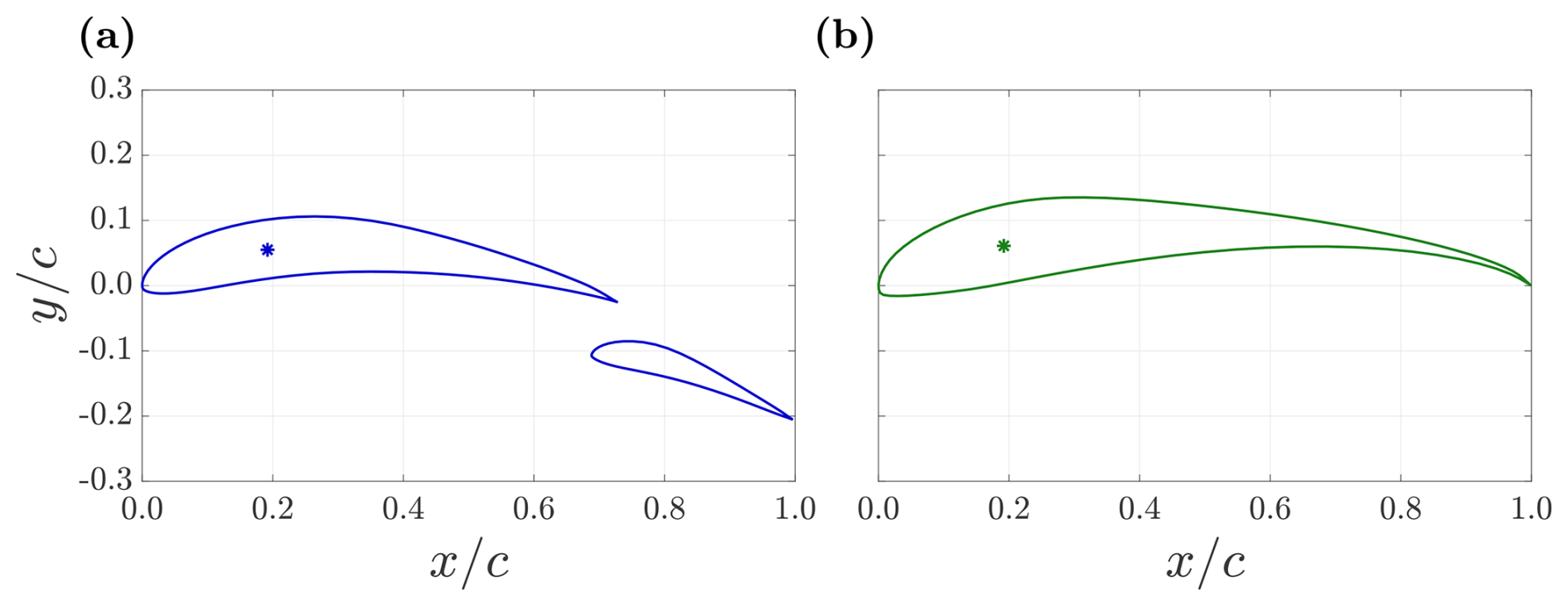
Figure B3 (a) The XY plot depicts the two-element airfoil used in this study, designed by Broertjes (2024) using the MSES optimization tool (Drela, 2015). This configuration consists of two E423 airfoils (Selig et al., 1997). (b) The XY plot shows the single-element airfoil S1223 (Selig et al., 1995), used as a reference to evaluate the performance of the two-element airfoil employed in this work. The pitching axes for both airfoils are indicated with ^* and are located at $(x/c=\mathrm{0.192},y/c=\mathrm{0.055})$ for the two-element airfoil and $(x/c=\mathrm{0.192},y/c=\mathrm{0.061})$ for the single-element airfoil.

Based on the $C_{\mathrm{l}}^{\mathrm{3}\mathrm{D}}$ results shown in Fig. B2, the maximum $C_{\mathrm{l}}^{\mathrm{3}\mathrm{D}}$ achieved by the wings with the two-element airfoil profile is approximately 25 % higher than that of the single-element airfoil. According to classic lifting-line theory (Anderson, 2011), increased lift is associated with stronger tip vortices, which in turn enhance the induced vertical velocity in the wake (commonly referred to as downwash). Note that stronger induced vertical velocity is considered beneficial for the performance of MRSLs (Li et al., 2025c). Therefore, despite the higher $C_{\mathrm{d}}^{\mathrm{3}\mathrm{D}}$ exhibited by the two-element airfoil, it is selected for the final MRSL design due to its superior lift characteristics, which provide aerodynamic advantages that could accelerate the downstream flow recovery.

B2 Selecting the pitch angles of the MRSL

The performance of the wing with the two-element airfoil profile, characterized by $C_{\mathrm{l}}^{\mathrm{3}\mathrm{D}}$ and $C_{\mathrm{d}}^{\mathrm{3}\mathrm{D}}$, is initially evaluated under freestream conditions. However, since the wings in the MRSL's model are expected to undergo significant aerodynamic interaction with the porous disk, it is necessary to measure the loads on the wings and the porous disk when they are assembled together. This approach enables the selection of appropriate pitch angles θ_p for the wings based on measured loads, with the objective of maximizing the wings' vertical (y-directional) forces.

To independently measure the loads on the wings and the porous disk, it is essential to eliminate any solid contact between the two components. This is accomplished using the setup shown in Fig. B1b. Additionally, because the relative positions of the wings and the disk are expected to influence their aerodynamic interaction, load measurements are conducted at every mounting position of the wings.

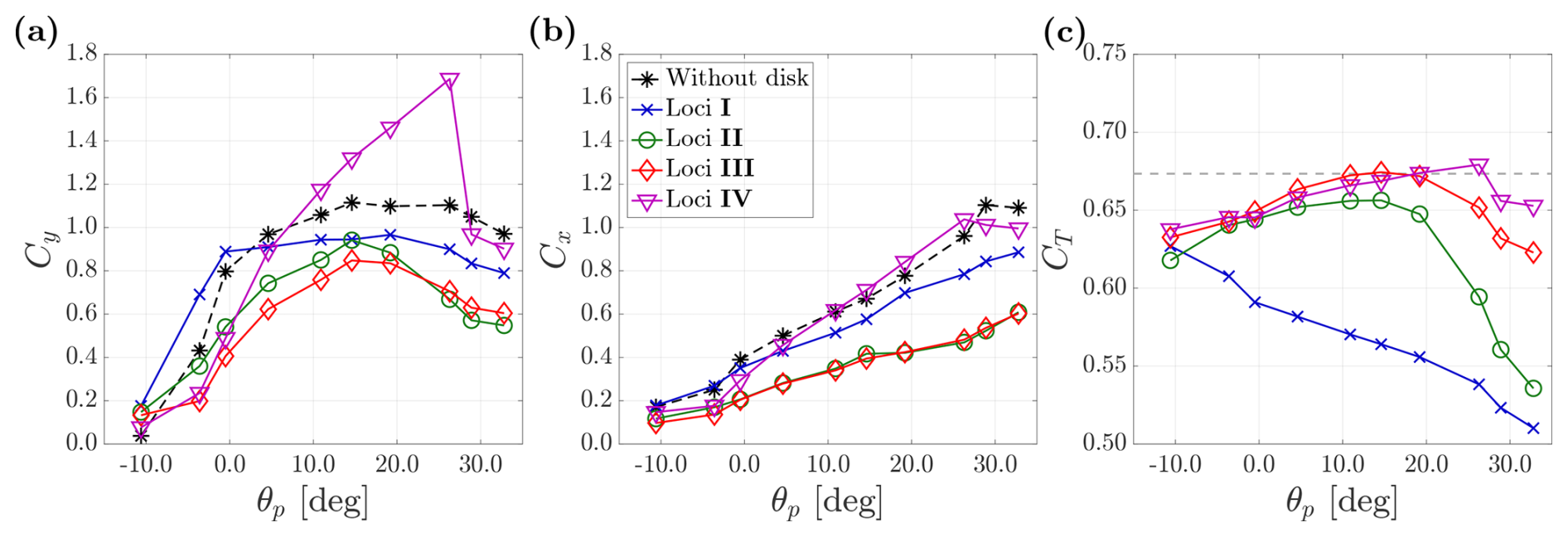
Figure B4 (a, b) Time-averaged three-dimensional wing loads measured in the presence of the porous disk, with porosity being 60 %. Note that only a single wing (two-element airfoil) is placed during the measurements, as depicted in the middle panel of Fig. B4. Wing loads are measured at different positions, with the loci positions illustrated on the right of Fig. B4. C_y and C_x denote the vertical and streamwise force coefficients, respectively, as defined in Eq. (B1). The uncertainties of C_x and C_y due to the load sensor are below 0.01, while the uncertainties in the pitch angle θ_p are approximately 1°. (c) The corresponding thrust coefficient C_T measured simultaneously with C_y and C_x. The dashed gray line indicates the C_T level for the disk without wings. The uncertainties in C_T due to the load sensor are below 0.03.

Prior to the experiment, it was already determined that the MRSL would be equipped with three wings and both up-washing and down-washing configurations would be investigated. Since the preliminary tests do not include the floor, some wing loci can be used for both configurations, reducing the number of required test positions to four. The positions of these loci are illustrated in Fig. B1c. Specifically, for the up-washing configuration, the wings are placed at loci IV, III, and II as the top, middle, and bottom wings, respectively. For the down-washing configuration, the wings are positioned at loci I, II, and III as the top, middle, and bottom wings, respectively. The positions of these four loci are located at $y/D=-\mathrm{0.05}$, 0.32, 0.68, and 1.05, with the origin placed at the edge of the disk on the negative y side.

The time-averaged three-dimensional wing's loads measured in the presence of the porous disk are displayed in Fig. B4a and b. Note that only one wing is installed at a time, and the porosity of the disk is 60 %. Here, C_y and C_x represent the vertical and streamwise force coefficients, respectively, as defined in Eq. (B1), with u_∞=8.0 m s⁻¹. $f_y^{\mathrm{W}}$ and $f_x^{\mathrm{W}}$ are the streamwise and vertical forces exerted by the wing. Notations of $C_{\mathrm{l}}^{\mathrm{3}\mathrm{D}}$ and $C_{\mathrm{d}}^{\mathrm{3}\mathrm{D}}$ are not used here, as the presence of the disk complicates and alters the inflow conditions, including the direction of the inflow. The results show that C_y for loci I, II, and III generally underperform compared to cases without the disk. This is expected, as the porous disk slows down the flow, reducing the forces, a trend also observed in C_x. Interestingly, C_y for locus IV significantly outperforms the case without the disk. This can be attributed to the fact that the wing at locus IV is not shadowed by the porous disk. Additionally, the blockage effect of the disk accelerates the flow and alters its direction, which further enhances C_y for locus IV compared to conditions without the disk.

$$\begin{array}{}\text{(B1)}& C_y\stackrel{\Delta }{=}{\displaystyle \frac{\left|f_y^{\mathrm{W}}\right|}{\mathrm{0.5}\mathit{\rho }{u}_{\mathrm{\infty }}^{\mathrm{2}}cD}},C_x\stackrel{\Delta }{=}{\displaystyle \frac{\left|f_x^{\mathrm{W}}\right|}{\mathrm{0.5}\mathit{\rho }{u}_{\mathrm{\infty }}^{\mathrm{2}}cD}}\end{array}$$

Regarding the maximum vertical force (maximum C_y) measured at different loci, it is observed that the maximum C_y for loci I, II, and III occurs around θ_p=15°, while for locus IV, it occurs at θ_p=25°. However, a significant drop in C_y is seen at locus IV when θ_p>25°, prompting a more conservative choice. Additionally, visualizing the flow field with smoke reveals severe flow separation at locus I when θ_p is set beyond 10°, which is only alleviated when θ_p≤5°. Based on these findings, the pitch angles for the final design are set as follows. For the up-washing configuration, θ_p for top, middle, and bottom wings are set at −15, −15, and −15°, respectively. As for the down-washing configuration, θ_p is set to 5, 15, and 15° for top, middle, and bottom wings, respectively. The values of θ_p given here are those used in the final design described in Sect. 2.2.

The thrust coefficient C_T of the porous disk, which is measured simultaneously with wing's C_y and C_x, is presented in Fig. B4c. The load sensor used for the disk is a unidirectional strain gauge (KD24s 10N, ME-Meβsysteme) capable of measuring tensile and compressive forces with a precision of 0.01 N. The sampling rate is set to 1000 Hz, and the sampling duration is 20 s. The plot shows that the load on the disk is generally higher when the wing is positioned at loci III or IV compared to loci I or II. This result aligns with expectations, as the bound circulation of the wing alters the flow field around the disk. When the wing is situated at loci III or IV, its circulation system tends to accelerate the flow over the disk, whereas the circulation of the wing at loci I or II slows the flow down.

Interestingly, despite the additional blockage and drag introduced by the wing, the presence of a wing at loci III or IV can result in higher loads on the disk compared to a stand-alone disk. This phenomenon is also observed in measurements of the thrust force for the up-washing configuration in Sect. 3.1. These observations highlight the significant aerodynamic interactions between the wings and the porous disk of the MRSL's model.

B3 Concluding remarks for preliminary experimental tests

The preliminary experiments provide valuable insights about the aerodynamic behaviors of the MRSL model and is critical in informing the final design used in the main study for farm-scale testing. Notably, three-dimensional PTV measurements are also conducted during these tests. While the PTV results contribute to the design decisions, they are not included in this appendix, as many of the key findings have already been covered in the main text. However, several interesting and potentially important aspects of the MRSL model remain unexplored, such as the wing–wing aerodynamic interactions within an MRSL. These topics are left for future investigations.

Appendix C: Algorithm for stitching and scaling the measured volumes

This appendix provides a detailed description of the stitching algorithm used to stitch the volumes measured with 3D-PTV. An overview of the stitching process is presented in the diagrams in Fig. C1, while the algorithm itself is described in detail from Eqs. (C1) to (C5). The scripts for executing stitching along with an example dataset are provided with the accompanying data repository (Li et al., 2025a).

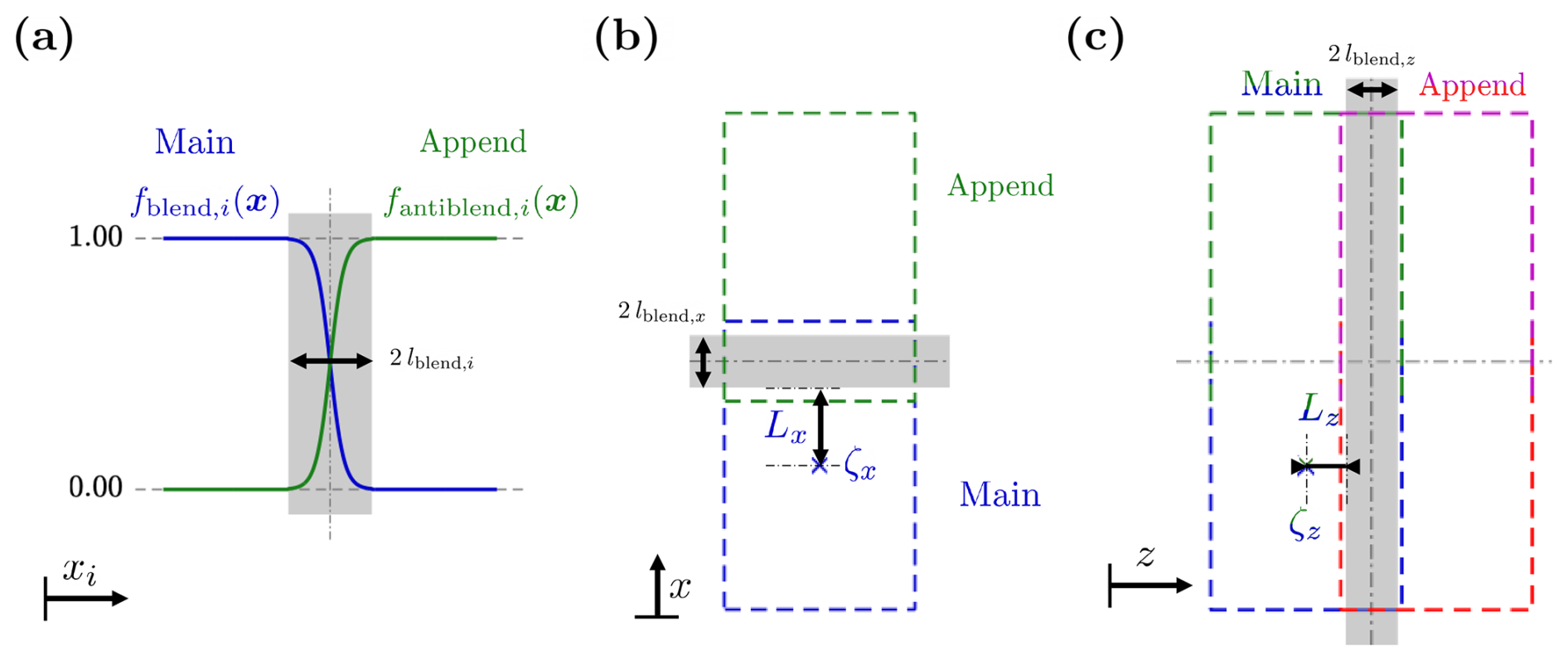
Figure C1 Schematic diagrams illustrating the stitching of measured volumes. The dashed lines in different colors represent the fields of view from different measurements. In the diagrams, volume Append is stitched onto volume Main, with the shaded areas indicating the blending regions. (a) Blending weights for volume Main and anti-blending weights for volume Append. (b) Stitching volume Append onto volume Main in the x direction. (c) Stitching another volume Append onto the existing volume in the z direction. Note that both Main and Append can represent volumes that have already been stitched together with several subvolumes.

During the stitching process, volumes are stitched recursively, as illustrated in Fig. C1b and c. It is important to note that the algorithm handles only one direction at a time, requiring the stitching sequence to be designed in advance.

In Fig. C1 and Eqs. (C1) to (C5), x represents the position vector of the point of interest, while ζ denotes the position vector of the stitching reference point within the volume Main, where the vector is used to determine the blending weightings. Throughout this appendix, the suffix i indicates the stitching direction, which in this work corresponds to x (streamwise direction) or z (lateral direction). The variable δ_i is the distance between x and ζ along the ith direction.

The blending weightings f_blend,i and f_antiblend,i are defined in Eqs. (C2) and (C3), respectively, and are described using a hyperbolic tangent function within the blending zone. The constant Λ_blend controls the rate of change of the blending weights, and in this work, Λ_blend=3 is used (note that tanh (3)>0.995). These blending weightings help to alleviate the potential spurious jumps in flow quantities due to stitching.

When stitching two volumes, the blending depth is defined as 2  l_blend,i. In this work, l_blend,x and l_blend,z are both set to 75 mm. This choice is based on the traverse system step size (${\mathrm{\Delta }}_{\mathrm{Tra},x}=\mathrm{600}$ mm and ${\mathrm{\Delta }}_{\mathrm{Tra},z}=\mathrm{375}$ mm) and the field of view dimensions (FOV_x=830 mm and FOV_z=550 mm), ensuring that the entire blending zone falls within the overlapping region of the two measurements. Specifically, the condition ${\mathrm{\Delta }}_{\mathrm{Tra},i}+\mathrm{2}{l}_{\mathrm{blend},i}<{\mathrm{FOV}}_i$ is satisfied for both the x and z directions. This is visualized in Fig. C1b and c. Note that $L_i\stackrel{\Delta }{=}({\mathrm{\Delta }}_{\mathrm{Tra},i}-\mathrm{2}{l}_{\mathrm{blend},i})/\mathrm{2}$.

$$\begin{array}{}\text{(C1)}& {\displaystyle }\mathit{\delta }\left(\mathit{x}\right)=\mathit{x}-\mathit{\zeta },{\mathit{\delta }}_i=x_i-{\mathit{\zeta }}_i\text{(C2)}& {\displaystyle }{f}_{\mathrm{blend},i}\left(\mathit{x}\right)=\left\{\begin{array}{l}\mathrm{1.00}\\ \mathrm{if}{\mathit{\delta }}_i\left(\mathit{x}\right)<L_i\\ \mathrm{0.00}\\ \text{if}{\mathit{\delta }}_i\left(\mathit{x}\right)>L_i+\mathrm{2}{l}_{\text{blend},i}\\ \mathrm{0.5}\left(\tanh \left[{\mathrm{\Lambda }}_{\mathrm{blend}}\left(\frac{L_i-{\mathit{\delta }}_i}{l_{\mathrm{blend}},i}+\mathrm{1}\right)\right]+\mathrm{1}\right)\\ \text{if}{L}_i\le {\mathit{\delta }}_i\left(\mathit{x}\right)\le L_i+\mathrm{2}{l}_{\mathrm{blend},i},\end{array}\right.\text{(C3)}& {\displaystyle }{f}_{\mathrm{antiblend},i}\left(\mathit{x}\right)=\mathrm{1}-f_{\mathrm{blend},i}\left(\mathit{x}\right)\end{array}$$

Before initiating the stitching process, the binned data are first interpolated onto a global grid shared by all volumes. The grid size of the global grid is comparable to the binning size. This step significantly facilitates the algorithm since the voxel sizes of different measurements may vary slightly due to re-calibration between measurements. After projecting the binned data onto the global grid, a layer equivalent to two grid sizes is trimmed from the edges to reduce noise before further processing.

An important consideration in the stitching process is that the volumes being stitched together are obtained from different measurements. Due to limitations of the wind tunnel, the jet wind speed is not perfectly consistent over the weeks-long experimental campaign, fluctuating between 7.2 and 7.4 m s⁻¹. To prevent spurious discontinuities, slight scaling of the flow properties is done during stitching. The scaling factor, denoted as Π, is calculated through Eq. (C4) based on the time-averaged streamwise velocity $\stackrel{\mathrm{‾}}{u}$ measured in the blending zone overlapped by the two volumes.

$$\begin{array}{}\text{(C4)}& \begin{array}{rl}& \mathrm{\Pi }=\left[\sum _{\begin{array}{c}\mathit{x}\in \mathrm{blending}\mathrm{zone}\\ min\left(N_{\mathrm{Main}},N_{\mathrm{Append}}\right)\ge {\mathrm{\Theta }}_N\\ y\ge {\mathrm{\Theta }}_y\end{array}}{\stackrel{\mathrm{‾}}{u}}_{\mathrm{Main}}min\left(N_{\mathrm{Main}},N_{\mathrm{Append}}\right)\right]\\ & /\left[\sum _{\begin{array}{c}\mathit{x}\in \mathrm{blending}\mathrm{zone}\\ min\left(N_{\mathrm{Main}},N_{\mathrm{Append}}\right)\ge {\mathrm{\Theta }}_N\\ y\ge {\mathrm{\Theta }}_y\end{array}}{\stackrel{\mathrm{‾}}{u}}_{\mathrm{Append}}min\left(N_{\mathrm{Main}},N_{\mathrm{Append}}\right)\right]\end{array}\end{array}$$

To minimize noise when calculating the values of Π, only the upper half of the blending region (y≥Θ_y, ${\mathrm{\Theta }}_y/D=\mathrm{0.2}$) is considered, as this region is generally less affected by the MRSL and exhibits lower turbulence. Additionally, a particle count threshold of Θ_N=10 is applied to ensure that Π is less influenced by noise (data are neglected if N<Θ_N).

Finally, with f_blend,i, f_antiblend,i, and Π, the stitching process can be performed. The stitching of a property B is described mathematically in Eq. (C5). Here, n_B represents the exponent of the scaling factor Π, and its value depends on the nature of B. This is necessary because Π is determined based on the streamwise velocity component u, regardless of what B represents. For velocity components (u, v, or w) or vorticity components (ω_x, ω_y, or ω_z), n_B=1. For properties such as turbulent kinetic energy or 2nd-order Reynolds stresses, n_B=2. Additionally, if B represents particle number N, n_B is set to 0, as no scaling is required.

$$\begin{array}{}\text{(C5)}& \begin{array}{rl}& B_{\mathrm{stitched}}\left(\mathit{x}\right)\\ & =\left\{\begin{array}{l}{B}_{\mathrm{Main}}\\ \mathrm{if}{\mathit{\delta }}_i\left(\mathit{x}\right)<L_i\\ {\mathrm{\Pi }}^{n_B}{B}_{\mathrm{Append}}\\ \mathrm{if}{\mathit{\delta }}_i\left(\mathit{x}\right)>L_i+\mathrm{2}{l}_{\mathrm{blend},i}\\ B_{\mathrm{Main}}\\ \mathrm{if}{L}_i\le {\mathit{\delta }}_i\left(\mathit{x}\right)\le L_i+\mathrm{2}{l}_{\mathrm{blend},i\mathrm{and}{N}_{\mathrm{Main}}\ge {\mathrm{\Theta }}_N\mathrm{and}{N}_{\mathrm{Append}}<{\mathrm{\Theta }}_N}\\ {\mathrm{\Pi }}^{n_B}{B}_{\mathrm{Append}}\\ \mathrm{if}{L}_i\le {\mathit{\delta }}_i\left(\mathit{x}\right)\le L_i+\mathrm{2}{l}_{\mathrm{blend}},i\mathrm{and}{N}_{\mathrm{Append}}\ge {\mathrm{\Theta }}_N\mathrm{and}{N}_{\mathrm{Main}}<{\mathrm{\Theta }}_N\\ \frac{B_{\mathrm{Main}}{N}_{\mathrm{Main}}{f}_{\mathrm{blend},\mathrm{i}}+{\mathrm{\Pi }}^{n_B}{B}_{\mathrm{Append}}{N}_{\mathrm{Append}}{f}_{\mathrm{antiblend},\mathrm{i}}}{N_{\mathrm{Main}}{f}_{\mathrm{blend},\mathrm{i}}+N_{\mathrm{Append}}{f}_{\mathrm{antiblend},\mathrm{i}}}\\ \mathrm{if}{L}_i\le {\mathit{\delta }}_i\left(\mathit{x}\right)\le L_i+\mathrm{2}{l}_{\mathrm{blend}},i\mathrm{and}{N}_{\mathrm{Main}}\ge {\mathrm{\Theta }}_N\mathrm{and}{N}_{\mathrm{Append}}\ge {\mathrm{\Theta }}_N\\ \mathrm{NaN}\left(\mathrm{setto}\mathrm{0}\mathrm{if}B\mathrm{is}N\right)\\ \mathrm{else}\end{array}\right.\end{array}\end{array}$$

After recursively stitching the measured volumes, the entire field of interest is obtained as an entity, resulting in a single stitched volume for each case. However, to facilitate comparisons between cases with different configurations of the regenerative wind farm, a final scaling step is required to account for slight variations in inflow velocity between cases (due to the wind tunnel). For this purpose, the property B of the stitched volumes is further multiplied by ${\mathrm{\Pi }}_{\mathrm{Global}}^{n_B}$, where Π_Global is determined in the inflow zone of the regenerative wind farm, as described in Eq. (C6). For the cases with the aligned layout, the inflow zone is defined within the region $-\mathrm{0.95}<x/D<-\mathrm{0.60}$, $\mathrm{0.53}<y/D<\mathrm{0.88}$, and $\mathrm{0.84}<z/D<\mathrm{1.20}$, and the reference inflow velocity is given as u_∞=7.3 m s⁻¹.

$$\begin{array}{}\text{(C6)}& \begin{array}{rl}{\mathrm{\Pi }}_{\mathrm{Global}}=u_{\mathrm{\infty }}& /\left[\left(\sum _{\begin{array}{c}\mathit{x}\in \mathrm{inflow}\mathrm{zone}\\ N_{\mathrm{stitched}}\ge {\mathrm{\Theta }}_N\end{array}}{\stackrel{\mathrm{‾}}{u}}_{\mathrm{stitched}}{N}_{\mathrm{stitched}}\right)\right.\\ & \left./\left(\sum _{\begin{array}{c}\mathit{x}\in \mathrm{inflow}\mathrm{zone}\\ N_{\mathrm{stitched}}\ge {\mathrm{\Theta }}_N\end{array}}{N}_{\mathrm{stitched}}\right)\right]\end{array}\end{array}$$

Appendix D: Further details on the vortex dynamics

This appendix complements Sect. 3.4, providing additional detail on the vorticity fields measured in this work. As in Sect. 3.4, the ${\stackrel{\mathrm{‾}}{\mathit{\omega }}}_x$ fields shown here have been filtered by spatial averaging within a spherical volume of radius 0.06D. Figure D1 presents three-dimensional iso-surfaces of ${\stackrel{\mathrm{‾}}{\mathit{\omega }}}_x$ for cases UW-05 and DW-05, while Figs. D2 and D3 show contour plots of ${\stackrel{\mathrm{‾}}{\mathit{\omega }}}_x$ for the same cases at additional x locations compared to Fig. 17. Together, these figures explicitly illustrate the spatial evolution of vortical structures between the successive rows of RGWFs.

For convenience, the parameter $x^{+,n\mathrm{th}}$ is introduced, which stands for the streamwise distance downstream away from the nth-row MRSL's x position. The mathematical definition of $x^{+,n\mathrm{th}}$ is given in Eq. (D1).

$$\begin{array}{}\text{(D1)}& \begin{array}{rl}& x^{+,n\mathrm{th}}\stackrel{\Delta }{=}x-x^{n\mathrm{th}},\\ & \mathrm{where}{x}^{n\mathrm{th}}\mathrm{is}\mathrm{the}x\text{-position}\mathrm{of}\mathrm{the}n\mathrm{th}\text{-row}\mathrm{MRSL}\end{array}\end{array}$$

Combining Figs. D1 to D3, the spatial evolution of the tip-vorticity structures for cases UW-05 and DW-05 is captured in detail. The tip vortices are clearly seen revolving around the swirling centers, with opposite rotational directions in UW-05 and DW-05. The merging and diffusion processes of the vortices are also evident. These plots show that by $x^{+,n\mathrm{th}}=\mathrm{4}D$, all three pairs of tip vortices have merged, except for those generated by the first-row MRSL in UW-05. In other words, the vortices have already merged before reaching the MRSL situated in the next row.

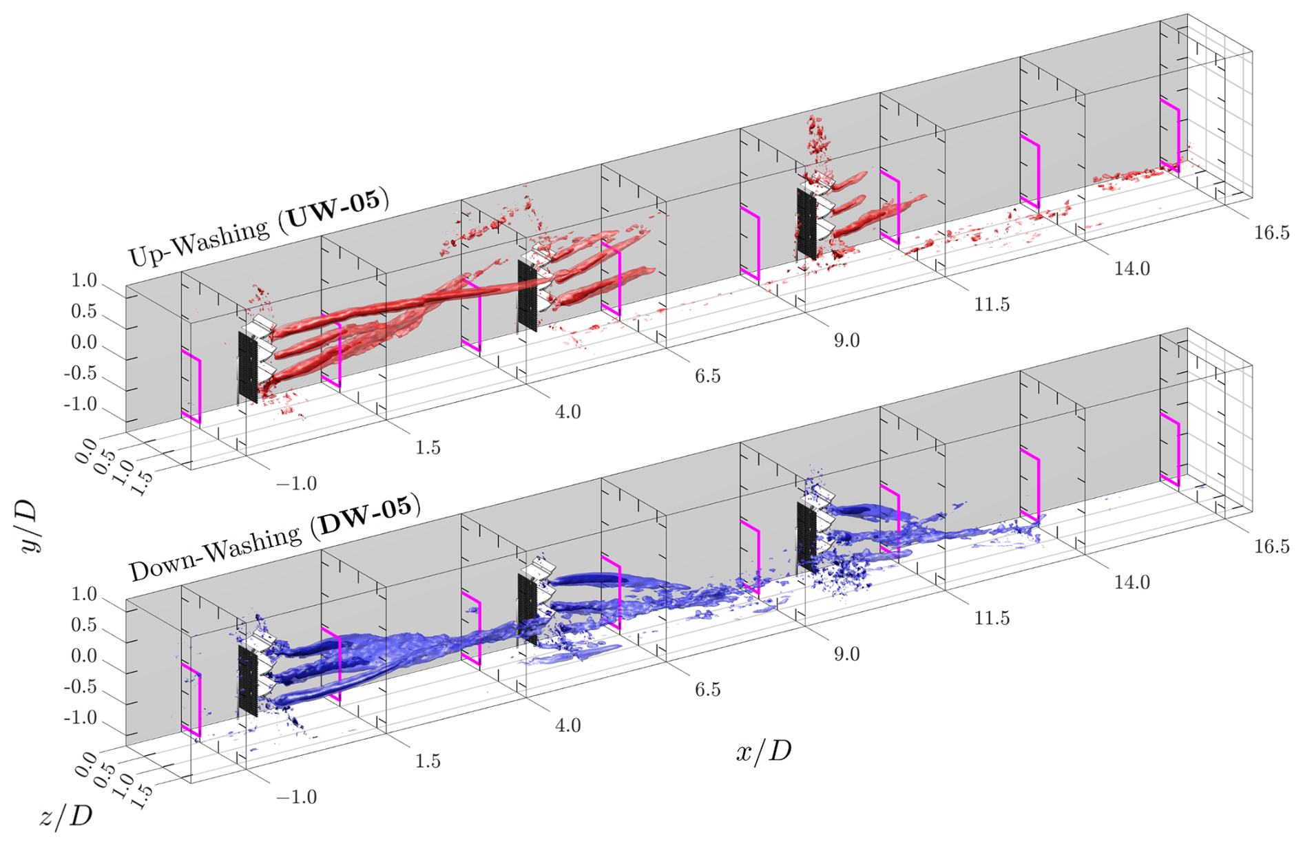
Figure D1 Iso-surfaces of the time-averaged streamwise vorticity (${\stackrel{\mathrm{‾}}{\mathit{\omega }}}_x$) for cases UW-05 and DW-05. Vorticity fields beyond the range $\mathrm{0.0}\le z/D\le \mathrm{1.4}$ are omitted for clearer presentation. The lighter and darker iso-surfaces correspond to iso-values of ±2 and ±4 for ${\stackrel{\mathrm{‾}}{\mathit{\omega }}}_{x}D/u_{\mathrm{\infty }}$, respectively, which is positive for UW-05 and negative for DW-05. The projected areas of the MRSLs are marked with magenta squares.

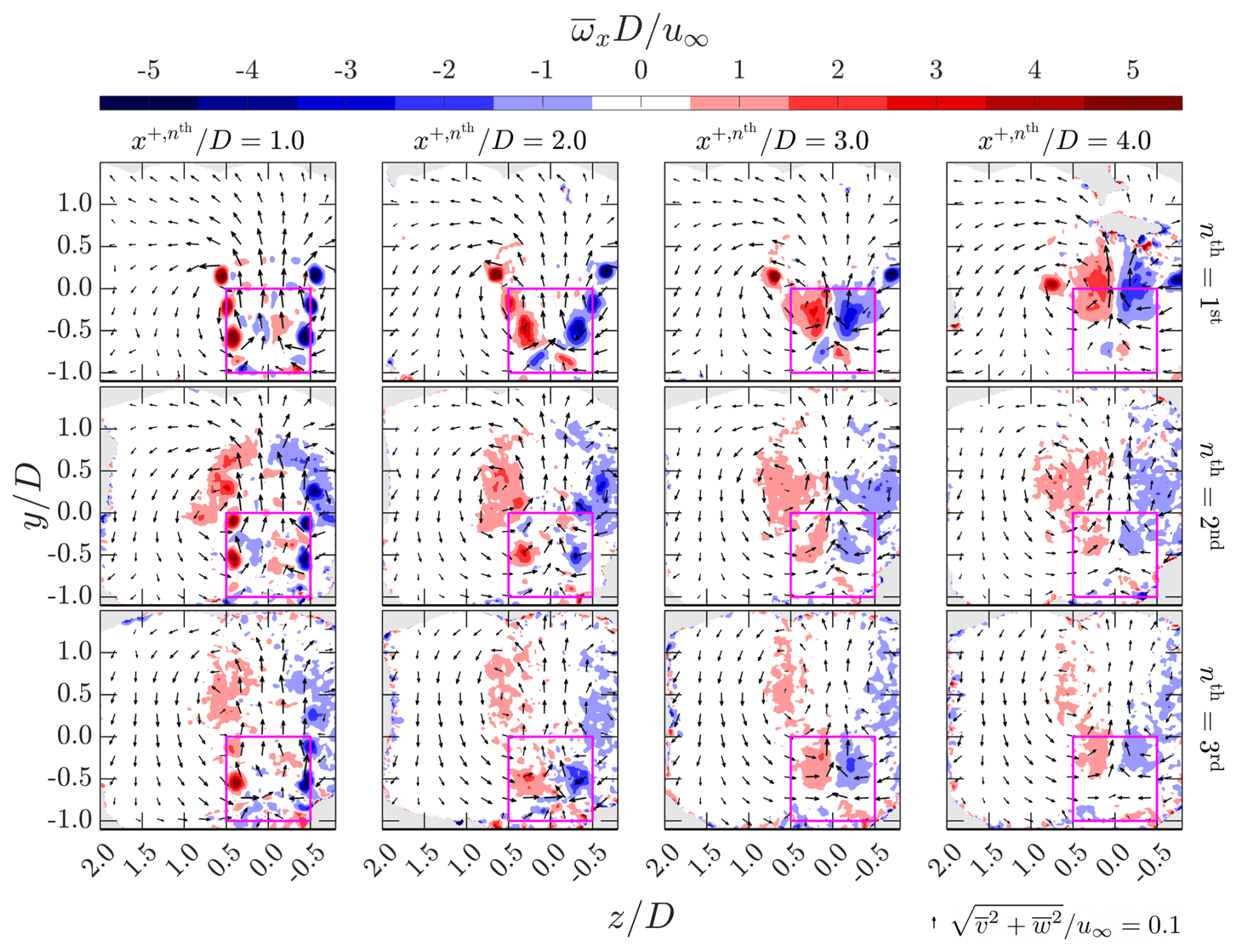
Figure D2 Contours of time-averaged streamwise vorticity (${\stackrel{\mathrm{‾}}{\mathit{\omega }}}_x$) for cases UW-05. The streamwise distance behind the nth-row MRSL is indicated at the top of each column and the row number is on the right of each row. Note that x^1st, x^2nd, and x^3rd are 0, 5, and 10D, respectively. The projected areas of the MRSLs are marked with magenta squares. In-plane velocity directions are illustrated by arrows, scaled according to their magnitudes. The reference scale for the arrows is provided in the bottom-right corner of the figure.

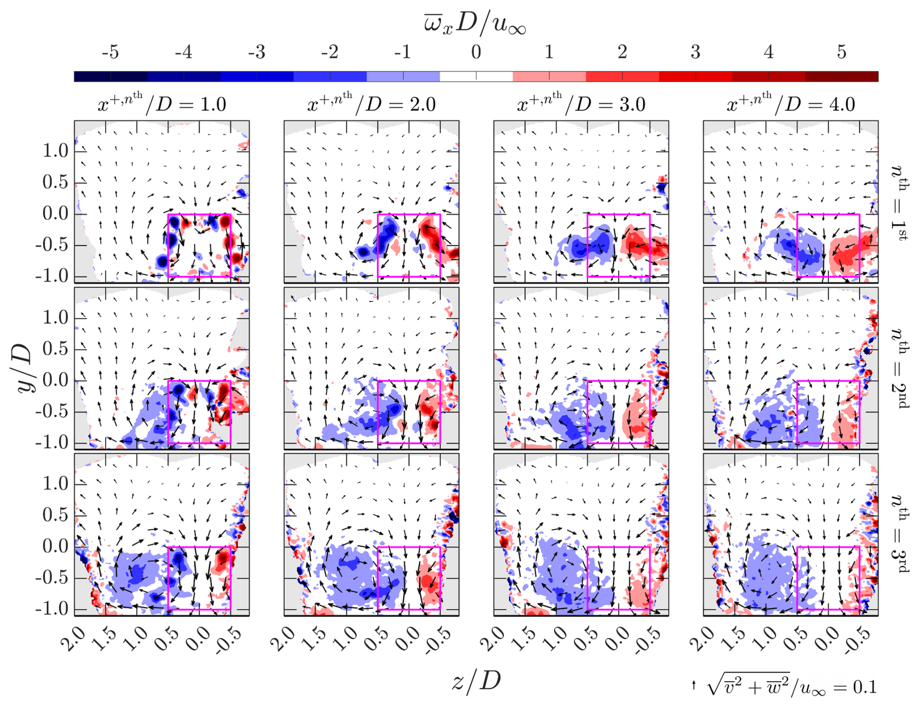
Figure D3 Contours of time-averaged streamwise vorticity (${\stackrel{\mathrm{‾}}{\mathit{\omega }}}_x$) for case DW-05. The streamwise distance behind the nth-row MRSL is indicated at the top of each column and the row number is on the right of each row. Note that x^1st, x^2nd, and x^3rd are 0, 5, and 10D, respectively. The projected areas of the MRSLs are marked with magenta squares. In-plane velocity directions are illustrated by arrows, scaled according to their magnitudes. The reference scale for the arrows is provided in the bottom-right corner of the figure.

Overall, the contour plots in this appendix show that the tip vortices in the case UW-05 diffuse more rapidly than those in DW-05. This observation is consistent with the LES results of Li et al. (2025b), although the setup in that study is only broadly comparable to the present work (see Sect. 3.6.2). This discrepancy in the diffusion rates may suggest that the presence of ground significantly influences the vortex dynamics of the MRSL's tip vortices and, in turn, the effectiveness of the lifting devices in enhancing vertical entrainment. However, further research is needed to confirm this phenomenon and to more precisely identify its underlying cause.

Taken together, these supplementary visualizations provide additional clarity on the evolution, merging, and diffusion of the MRSL's tip vortices, consolidating the trends discussed in Sect. 3.4.