Periods of constant wind speed: how long do they last in the turbulent atmospheric boundary layer?

We perform a statistical analysis of the occurrence of periods of constant wind speed in atmospheric turbulence. We hypothesize that such periods of constant wind speed are related to characteristic wind field structures that, when interacting with a wind turbine, may induce particular dynamical responses. Therefore, this study focuses on characterizing the constant wind speed periods in terms of their lengths and probability of occurrence. Atmospheric offshore wind data are analyzed. Our findings reveal that long constant wind speed periods are an intrinsic feature of the marine atmospheric boundary layer (ABL). We confirm that the probability distribution of such periods of constant wind speeds follows a Pareto-like distribution, admitting power law behavior for periods exceeding the large-eddy-turnover time. The power law characteristics depend on the local conditions and the precise definition of wind speed thresholds. A comparison to wind time series generated with standard synthetic wind models and to time series from ideal stationary turbulence suggests that these structures are not characteristics of small-scale turbulence but seem to be consequences of larger-scale structures of the atmospheric boundary layer and thus are multi-scale. Given the results, we show that the continuous-time random walk (CTRW) model, as a non-standard wind model, can be adapted to generate time series of the wind speed whose statistics match the statistics of observed periods of constant wind speed.

1 Introduction

Estimation of the loads experienced by a wind turbine (WT) is fundamental to decision-making processes during the design phase of various components of the machine, as well as for control strategies during its operation. Such estimation is performed through numerical modeling of the interaction between the WT and the incoming wind. Therefore, an accurate description of the wind within the atmospheric boundary layer (ABL) is essential to correctly calculate the loads acting on the WT. The International Electrotechnical Commission (IEC) has defined both the widely used standard parameters for the characterization of the atmospheric wind and the models for generating synthetic wind fields used for numerical estimation of loads on the WT (IEC, 2019). These IEC standards consider the spectral properties and coherence of the velocity components of the wind. Nevertheless, such guidelines are designed to mimic the atmospheric wind in a computationally efficient way. As a result, some flow features in the ABL are neglected or simplified in the characterization of atmospheric measured data, as well as in the generation of the synthetic wind fields. Furthermore, during the past decades, new challenges in the design process of WTs have emerged (Veers et al., 2019). On the one hand, trends in the design of modern WTs account for bigger rotor areas and less rigid structures (i.e., blades) to capture more energy from the available wind resources. On the other hand, the weight and material requirements of each component are being pushed to minimal levels. As a result, new WTs are becoming, in general, larger and less rigid. Therefore, some of the characteristics of the wind within the ABL that are not addressed in the IEC standard wind models might become relevant for the extra loads that were previously neglected within the design of smaller and stiffer WTs.

Based on cooperative research with a WT manufacturer, we hypothesized that one of these features, disregarded by the IEC guidelines, is the periods of constant wind speed (CWS) in atmospheric flows. Such periods are defined as the intervals of time over which the magnitude of the wind speed remains almost constant within a certain range, limited by a threshold value. In the following, we first contextualize the periods of CWS within the general characterization of turbulent features. Afterwards, we discuss the ways in which such CWS structures may be relevant for a WT.

Concerning the CWS periods as a general feature of the wind, we should mention that there are relevant and well-investigated turbulent quantities closely associated with our definition of CWS periods. This is the case for the persistence phenomenon, which characterizes how long the flow remains in a particular state before switching to another one. Persistence times can be inversely related to occurrence rates of extreme wind speeds or gusts. In this context, the exceedance statistics proposed by Rice (1944) have been applied to describe gusts as excursions at which certain thresholds of wind speed are exceeded (Kristensen et al., 1991; Young and Kristensen, 1992; Manshour et al., 2016). Another interpretation of persistence within turbulent flows is the zero-crossing analysis. In this case, for a zero-mean signal, the waiting times between two successive crossings of its zero level are evaluated. Statistical properties of zero crossings have been used to characterize intrinsic turbulent quantities such as the Taylor micro-scale (Narayanan et al., 1977; Sreenivasan et al., 1983; Kailasnath and Sreenivasan, 1993; Poggi and Katul, 2010) or the integral length scale (Mora and Obligado, 2020; Mazellier and Vassilicos, 2008). Analyses of zero crossings of velocity and temperature fluctuations in atmospheric turbulent data have been discussed (Cava and Katul, 2009; Cava et al., 2012; Chamecki, 2013; Chowdhuri et al., 2020). To summarize, the above-mentioned investigations showed that the statistical characteristics of the persistence for experimental and atmospheric data exhibit power law behavior up to a certain threshold, followed by log-normal or exponential cutoffs.

It is worth noting that even though the inter-arrival times of both excursions and zero crossings refer to structures between particular turbulent states, they do not correspond to the periods of reduced turbulent amplitudes in which we are interested. Further details of the differences between CWS periods and inter-arrival times between excursions and zero crossings are shown in Appendix A. Nevertheless, the method and statistics of such persistent events are relevant to the discussion. Of special interest are self-similar, critical, or fractal features of turbulence that propose power law behavior for the probability distribution of the time intervals with duration T, which can be formulated as $p\left(T\right)\propto T^{-\mathit{\alpha }}$ (in particular for the limit of large T). A characteristic feature of a power law distribution is the absence of an intrinsic scale, i.e., the probability of observing a realization larger than ξT is ${\mathit{\xi }}^{-\mathit{\alpha }+\mathrm{1}}$ times the probability of observing a realization larger than T, independent of the value of T. The long-tail regime of many distributions occurring in complex systems is assumed to exhibit power law behavior (Laherrere and Sornette, 1998). In the context of wind energy, for instance, a Pareto distribution has been tested as an extrapolation method to estimate extreme loads on a multi-megawatt wind turbine generator with a 1-month return period (Dimitrov, 2016).

Next, we discuss the potential relevance of an accurate description of the CWS periods for WT applications, which is directly linked to the increasing size and flexibility of the WTs. In the simplest case, such periods of CWS should imply relatively quiescent operating conditions for a WT when the CWS structure occurs homogeneously in the rotor area. A more entangled case might occur when resonant or near-resonant dynamics appear for specific periods of CWS over which the resonance can be strongly excited. In particular, for the larger WTs, the CWS periods may be restricted to a sub-area of the rotor plane. In this case, resonant dynamics exhibiting 3P oscillations may be amplified. Within this context, recent studies are devoted to interfaces between turbulent and non-turbulent states in atmospheric wind measured at typical WT heights (Neuhaus et al., 2024). Meanwhile, numerical and experimental investigations of the laminar–turbulent transition mechanisms on rotating wind turbine blades have shown changes in the transition characteristics over a single revolution, which affect the aerodynamic response of the WT (Lobo et al., 2023; Özçakmak et al., 2020).

As a last possible application for WTs, we want to mention that the statistical features of CWS periods may become of interest for probabilistic design methods. Although the methods proposed by the IEC for estimating WT loads are mostly deterministic (IEC, 2019), in recent years, probabilistic design methods have been introduced as surrogates for the design and load assessment of WTs (Abhinav et al., 2024; Kelma, 2024). Such probabilistic approaches produce more reliable estimations by considering the explicit calculation of the uncertainties from the operational conditions, aerodynamic models, materials, etc. (Sørensen and Toft, 2010). Characteristics of the wind are then defined as stochastic variables within the probabilistic model. Accordingly, broader and more accurate statistical descriptions of the intrinsic features of the wind inside the ABL account for a reduction in the uncertainty in the estimated loads and responses of the WTs.

In this paper, we focus on the periods of CWS as general features of turbulence; the discussion of possible impacts on a WT will be done only as side remarks. In particular, we characterize the statistics of periods of CWS (with a low level of turbulent fluctuations) from wind measurements in the ABL. In a preliminary investigation, the method for the assessment of such events from wind speed time series was presented, and the first results on the characterization of the periods of CWS in terms of their duration and probability distributions were also reported (Moreno et al., 2022). Special attention within the characterization was given to the tails of the distributions, which describe extremely long periods. Interestingly, we found that the probability distribution for very long periods shows a power law decay $p\left(T\right)\propto T^{-\mathit{\alpha }}$. Furthermore, a comparison with wind data generated by an IEC standard model revealed that the model underestimates the frequency of occurrence of the extremely long CWS periods measured in the ABL. In this study, we aim to address whether the CWS periods are induced by specific orographic perturbations, whether they are laminar or low-turbulence structures, and whether they are intrinsic features of a turbulent flow or rather result from large-scale interactions within the ABL. To characterize the CWS periods, we use data from offshore wind, as we expect them to have fewer special orographic effects compared to onshore data, and thus we can get more general insights into the CWS structure. This is also the motivation for the comparison of our results with ideal turbulent data from a free-jet experiment. Furthermore, a stochastic wind field model for WT simulations is presented as a surrogate approach to incorporate the statistics of long CWS periods from turbulence in the ABL.

The paper is structured as follows: Sect. 2 restates the method for measuring the periods and describes the atmospheric wind data to be analyzed. In Sect. 3, the results of the statistical characterization of the periods from the atmospheric data are shown. In Sect. 4, we compare the results from ABL data to those from two different data sets, i.e., the IEC standard wind model and experimental ideal turbulence. In Sect. 5, we present our conclusions and potential future work.

2 Methodology and data

2.1 Definition of a period of CWS

Following Moreno et al. (2022), a CWS period (T_c) is defined as the time over which the magnitude of the wind speed u(t) exhibits low-amplitude fluctuations enclosed within certain thresholds. A period T_c is depicted in Fig. 1. Over the length of T_c, the wind speed remains inside the constant speed range (CSR). The CSR is defined as $u_{t^{*}}\pm \mathit{\epsilon }$, where $u_{t^{*}}$ is the reference speed value at $t=t^{*}$, and ε is the maximum acceptable magnitude of the fluctuations around $u_{t^{*}}$. In Fig. 1, the horizontal red bars illustrate the thresholds that delineate the CSR. It should be noted that the CWS periods are not strictly laminar but are periods with a smaller amplitude of turbulence; see also the spectral analysis in Sect. 3.

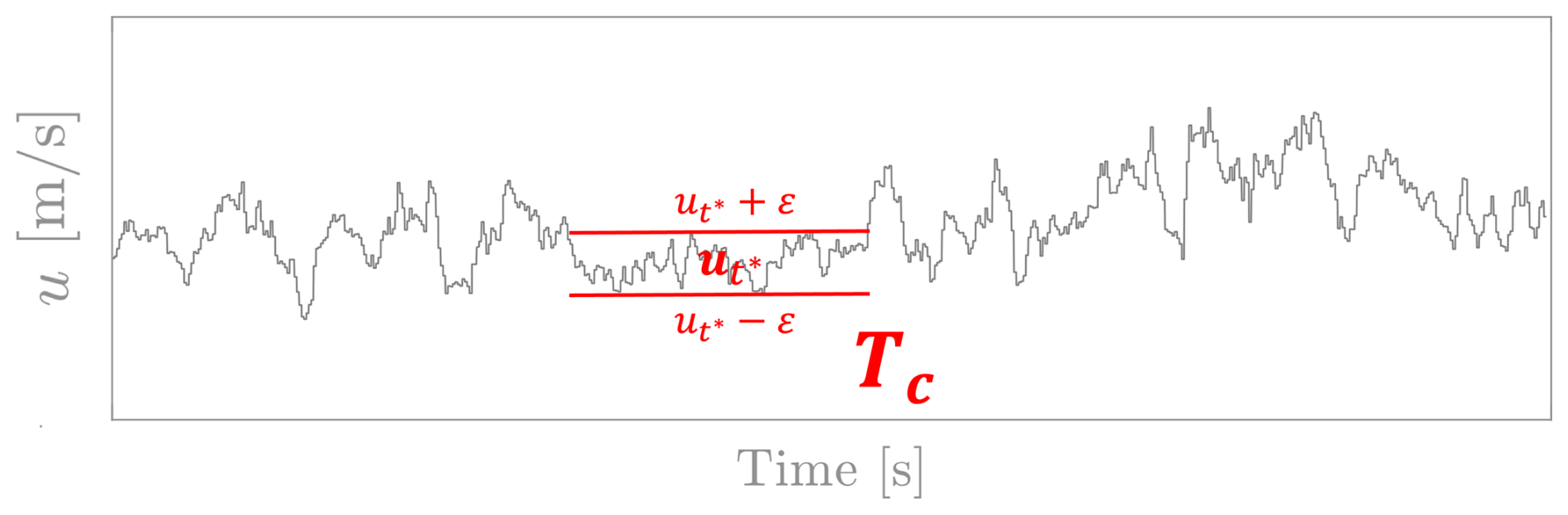
Figure 1 Schematic representation of a CWS period (T_c) measured from an exemplary wind speed time series u(t). The constant speed range (CSR), $u_{t^{*}}\pm \mathit{\epsilon }$, specifies the limits for the accepted level of turbulence within a period T_c. The CSR is shown by the horizontal red bars.

In the following, the method for measuring the length of a period T_c at a given time step t^* is described in detail. The goal is to count the number of N consecutive time steps, including t^*, for which their wind velocity u(t) is contained inside the CSR. For that, the reference speed $u_{t^{*}}=u\left(t^{*}\right)$ and the corresponding CSR, $u_{t^{*}}\pm \mathit{\epsilon }$, are defined. Next, the velocities at the time step $t^{*}+i$ for $i=(\mathrm{1},\mathrm{2},\mathrm{3}$…,∞) are evaluated and counted. The counter ${\stackrel{\mathrm{̃}}{N}}^{+}$ for the evaluation of $u_{t^{*}+\mathrm{1}}=u(t^{*}+i)$ is then defined as

$$\begin{array}{}\text{(1)}& {\stackrel{\mathrm{̃}}{N}}^{+}=\left\{\begin{array}{ll}{\stackrel{\mathrm{̃}}{N}}^{+}=+\mathrm{1}& \text{if}(u_{t^{*}}-\mathit{\epsilon })\le u_{t^{*}+\mathrm{1}}\le (u_{t^{*}}+\mathit{\epsilon })\\ \text{end}& \text{otherwise}.\end{array}\right.\end{array}$$

Note that only consecutive points are counted in ${\stackrel{\mathrm{̃}}{N}}^{+}$. The count is concluded once the value of $u(t^{*}+i)$ exceeds either the bottom limit or the top limit of the CSR. So far, only points in the forward direction (+) from t^* are evaluated. The same algorithm is subsequently applied to count the number of points ${\stackrel{\mathrm{̃}}{N}}^{-}$ in the backward direction from t^*. In this case, values of $i=(-\mathrm{1},-\mathrm{2},-\mathrm{3}\mathrm{\dots },-\mathrm{\infty })$ are considered to evaluate $u_{t^{*}+\mathrm{1}}$ in Eq. (1). Finally, the total number of consecutive points N measured at t^* results from the sum of ${\stackrel{\mathrm{̃}}{N}}^{+}$ and ${\stackrel{\mathrm{̃}}{N}}^{-}$, which are independently counted in their corresponding directions. The length of the period T_c at t^* is then obtained by multiplying the total N by the size of the time step δt. A period T_c is estimated for every time step in the time series u(t). In the case of overlapping periods, only the longest period measured is recorded. By doing so, a recounting of events is avoided.

In Moreno et al. (2022), the threshold ε for fixing the CSR, $u_{t^{*}}\pm \mathit{\epsilon }$, was randomly selected (e.g., 0.2–0.4 m s⁻¹), and the method described in Eq. (1) was applied over the actual measurements u(t). However, limitations of the method appear when analyzing large data sets with very different mean wind speed $\stackrel{\mathrm{‾}}{u}$ and standard deviation σ_u, which are calculated over shorter time windows (i.e., 10 min) with respect to the length of the sample. To introduce a systematic approach, in this paper, the threshold ε is defined as proportional to the standard deviation of the wind speed σ_u. Then, ε to fix $u_{t^{*}}\pm \mathit{\epsilon }$ is calculated as

$$\begin{array}{}\text{(2)}& \mathit{\epsilon }=A{\mathit{\sigma }}_u,\end{array}$$

where A is a factor, typically A<1. The value of A can be chosen depending on the particular application. In the case of a WT, A might be related to the thresholds for the control system to operate within different turbulent regimes. In practice, such thresholds in the operating protocols are commonly defined as a function of the turbulence intensity TI $={\mathit{\sigma }}_u/\stackrel{\mathrm{‾}}{u}$. In Eq. (2) and through this paper, we refer to $\stackrel{\mathrm{‾}}{u}$ and σ_u as the mean and standard deviation values calculated over 10 min periods, unless a distinction is clearly stated.

2.2 Atmospheric wind data

Data from the offshore research platform FINO (Forschungsplattformen in Nord- und Ostsee) are investigated. We expect offshore wind to provide a better representation of undisturbed, or less disturbed, conditions within the ABL compared to onshore data. Therefore, the possible effects of onshore orographic conditions on the CWS structures are diminished.

Specifically, measurements at the FINO1 platform, located in the North Sea, are used. Records of the wind speed u(t) were taken by vertically aligned cup anemometers mounted at different heights H (FINO, 2025). The data correspond to measurements from January to December 2007, with a sampling frequency of 1 Hz. Measurements at heights H=[ 30, 50, 70, 90] m above the mean sea level are considered. Wind speed records have been limited to those 10 min periods with $\stackrel{\mathrm{‾}}{u}$ between 3 and 25 m s⁻¹ due to their relevance for WT operation. Values of u(t) outside this range have been neglected. Moreover, to avoid disturbance from the met mast, data for wind directions between 275 and 350° are not considered. As an overview of the complete data set, Fig. 2 shows the mean $\stackrel{\mathrm{‾}}{u}$ and standard deviation σ_u calculated over individual 10 min periods at H=90 m.

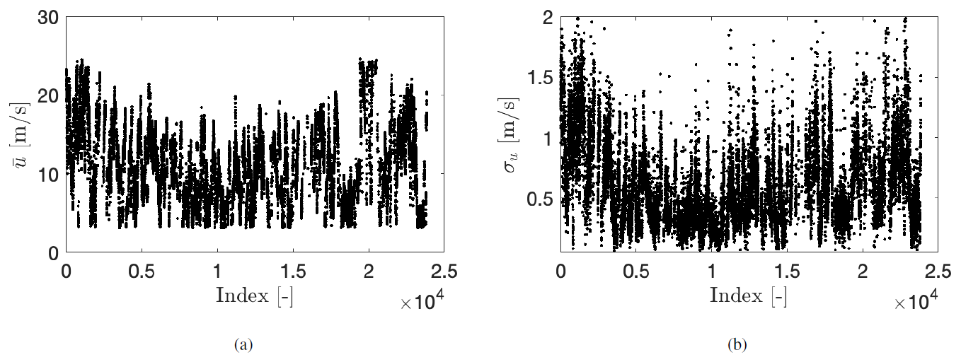
Figure 2 Wind velocity statistics of atmospheric FINO data at H=90 m. (a) Mean wind speed $\stackrel{\mathrm{‾}}{u}$. (b) Standard deviation σ_u. Each dot in the plots corresponds to a calculated value over a single 10 min period. The dots are chronologically ordered.

3 Statistics of T_c for atmospheric turbulent data

3.1 Mean, standard deviation, and maximum value of T_c

As a starting point for the statistical characterization of the measured CWS periods T_c, we discuss their mean duration (${\stackrel{\mathrm{‾}}{T}}_{\mathrm{c}}$), standard deviation (${\mathit{\sigma }}_{T_{\mathrm{c}}}$), and maximum value (T_c,max). We define T_c,max as a representative value from a set of the longest periods measured rather than the absolute and unique longest event. More details follow in Sect. 3.2. We compare the statistics of T_c at different heights H. A factor A=0.3 is chosen as an example to define the threshold ε=A σ_u for the CSR, $u_{t^{*}}\pm \mathit{\epsilon }$. The results are summarized in Table 1.

Table 1 Mean (${\stackrel{\mathrm{‾}}{T}}_{\mathrm{c}}$), standard deviation (${\mathit{\sigma }}_{T_{\mathrm{c}}}$), and maximum length (T_c,max) of the calculated periods T_c at different heights H. A factor A=0.3 is assumed for the estimation of T_c.

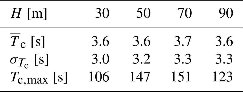
As a remark, special attention has to be devoted to the meaning of the statistical moments ${\stackrel{\mathrm{‾}}{T}}_{\mathrm{c}}$ and ${\mathit{\sigma }}_{T_{\mathrm{c}}}$ calculated from the data. In certain cases, such as those presented in Moreno et al. (2022), the probability distribution p(T_c) may lead to non-converging moments, e.g., mean and variance. Further details are discussed in Appendix B and C. From the values in Table 1, comparable ${\stackrel{\mathrm{‾}}{T}}_{\mathrm{c}}\approx \mathrm{4}\text{s}$ and ${\mathit{\sigma }}_{T_{\mathrm{c}}}\approx \mathrm{3}\text{s}$ are obtained for the four heights H. More interesting are the longest CWS periods measured T_c,max at each height H. Periods with lengths up to $T_{\mathrm{c}}\approx \mathrm{40}{\mathit{\sigma }}_{T_{\mathrm{c}}}$ that correspond to more than 100 s are measured. The specific values of ${\stackrel{\mathrm{‾}}{T}}_{\mathrm{c}}$, ${\mathit{\sigma }}_{T_{\mathrm{c}}}$, and T_c,max are expected to be dependent on the specific local conditions due to surface interactions. In particular, stronger differences in the lengths of CWS periods might arise under onshore conditions, as observed by Kelly (2024) when analyzing coastal flow accelerations at different heights.

3.2 Probability density function of T_c

Next, in the statistical characterization of the CWS periods, the probability density functions (PDFs) p(T_c) are discussed. Figure 3 shows p(T_c) for the data in Table 1 for different heights H. As mentioned before, we focus our attention on characterizing very long periods of T_c. Therefore we concentrate on the tails of p(T_c). For comparability, the values of T_c are normalized by the longest period measured at each H; more precisely, we use a representative value T_c,max of at least 10 of the longest periods to become more statistically robust. The values obtained for T_c,max are those summarized in Table 1.

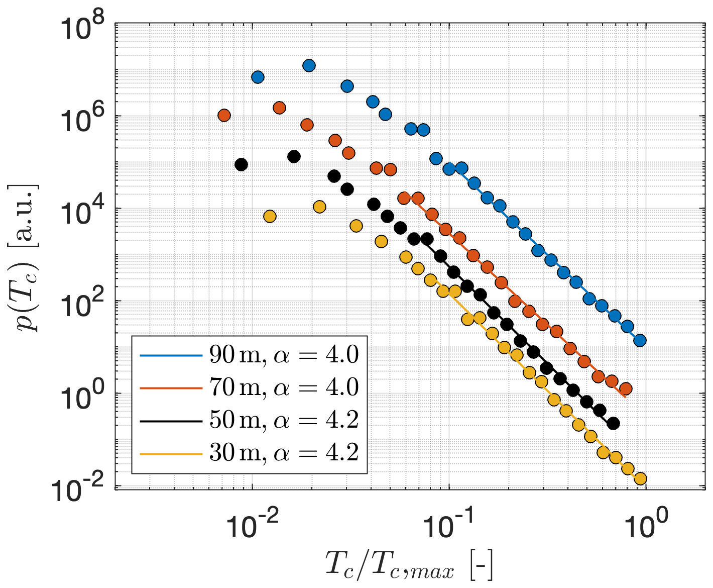
Figure 3 Normalized probability density functions $p(T_{\mathrm{c}}/T_{\mathrm{c},\max })$ for FINO data at different heights H. The dots illustrate the results from the FINO data. The solid lines show the power law decay fitting $\propto T_{\mathrm{c}}^{-\mathit{\alpha }}$. The value T_c,max for each height is defined as the bin center containing at least 10 of the longest periods measured after a binning process. The individual distributions are vertically shifted for better visualization.

The normalized PDFs p(T_c) in Fig. 3 are presented on a log–log scale. In such a representation, a straight line reveals power law behavior of the form $p\left(T_{\mathrm{c}}\right)\propto T_{\mathrm{c}}^{-\mathit{\alpha }}$, with α as the characteristic exponent. In Fig. 3, the power laws fitted over the tails of the distributions are shown by solid lines, with the same color used for the dots at each H. This indicates that the PDFs of CWS periods p(T_c) follow a Pareto-like distribution for large T_c (Laherrere and Sornette, 1998). We emphasize that the power laws extend over more than 1 decade. The corresponding exponents α are calculated following the procedure proposed by Clauset et al. (2009) and described in Appendix D. The values of α are given in the legends of the figure.

The variation in the exponent α for all H is within ±6 %.

This shows that the decay $p\left(T_{\mathrm{c}}\right)\propto T_{\mathrm{c}}^{-\mathit{\alpha }}$ does not depend on the height. Moreover, since α≥3 for all H, the second-order statistical moments of T_c converge, and the results presented in Table 1 provide meaningful information about the characteristics of the periods T_c (see Appendix B and C).

The power law behavior observed in the distributions p(T_c) for the offshore data shown in Fig. 3 agrees with the data obtained for the two onshore sites investigated by Moreno et al. (2022), as well as for analyses performed on data from the mast Wettermast Hamburg (2025). This indicates that the CWS structures T_c are not due to the specific orographic conditions but rather represent general characteristics of the ABL. However, as the actual values of the statistics of CWS periods (i.e., ${\stackrel{\mathrm{‾}}{T}}_{\mathrm{c}}$, ${\mathit{\sigma }}_{T_{\mathrm{c}}}$, T_c,max, α) vary significantly between data sets, they should be considered individually for each location.

3.3 Validity of the power law $p\left(T_{\mathrm{c}}\right)\propto T_{\mathrm{c}}^{-\mathit{\alpha }}$

To validate the universality of the power law distribution $p\left(T_{\mathrm{c}}\right)\propto T_{\mathrm{c}}^{-\mathit{\alpha }}$, we investigate the effect of the width of the CSR, $u_{t^{*}}\pm \mathit{\epsilon }$. Different values of the factor A, such as ε=A σ_u, are evaluated. The results of ${\stackrel{\mathrm{‾}}{T}}_{\mathrm{c}}$, ${\mathit{\sigma }}_{T_{\mathrm{c}}}$, T_c,max , and α for $A=[\mathrm{0.2},\mathrm{0.3},\mathrm{0.5},\mathrm{0.8}]$ are summarized in Table 2. Figure 4 shows the normalized PDFs p(T_c) in an analogue representation, as shown previously in Fig. 3.

Table 2 Mean (${\stackrel{\mathrm{‾}}{T}}_{\mathrm{c}}$), standard deviation (${\mathit{\sigma }}_{T_{\mathrm{c}}}$), maximum length (T_c,max), and exponent α of the T_c periods calculated for different values of the factor A. FINO measurements at H=90 m are analyzed.

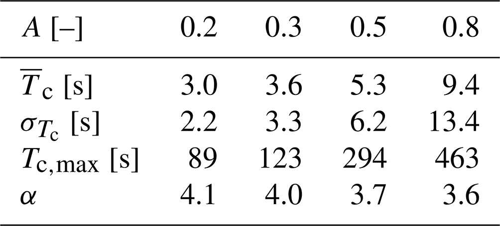
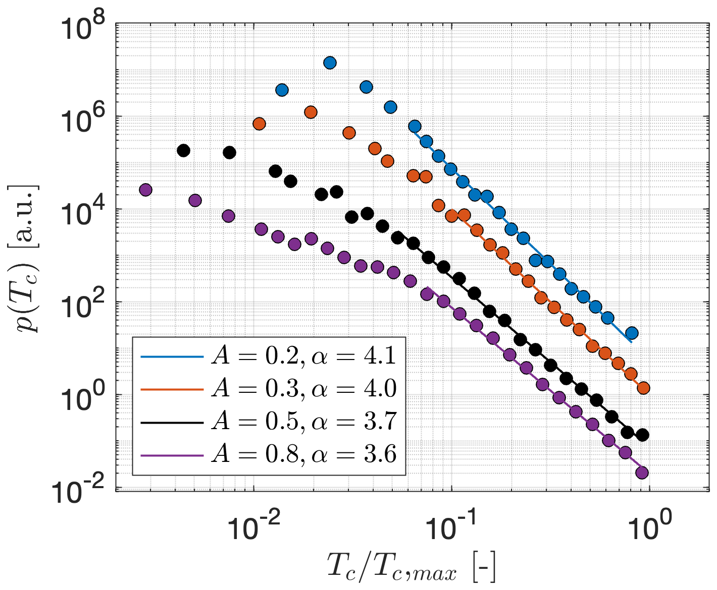
Figure 4 Normalized probability density functions $p(T_{\mathrm{c}}/T_{\mathrm{c},\max })$ for FINO data for different values of A. The power law fittings $\propto T_{\mathrm{c}}^{-\mathit{\alpha }}$ are depicted by the solid lines. Measurements at H=90 m are considered. The value T_c,max for each value of A is defined as the bin center containing at least 10 of the longest periods measured after a binning process. The individual distributions are vertically shifted for better visualization.

The tails of the PDFs in Fig. 4 show a clear power law decay $\propto T_{\mathrm{c}}^{-\mathit{\alpha }}$ for all values of A. This confirms our hypothesis about the Pareto-like distributions of p(T_c) for large T_c, which has already been observed in Fig. 3. Interesting to note is that the exponent α decreases with increasing width of the CSR or of the factor A.

3.4 Power spectra of u(t) during periods T_c

Further in the characterization of the CWS periods, the spectral features of the wind speed u(t) during the CWS periods T_c address the question of whether the wind speed is strictly laminar or is instead turbulent with a low degree of turbulence. The turbulent nature of u(t) is now verified by the power spectra shown in Fig. 5. The spectra E(f) are calculated from the time series of u(t) extracted during CWS periods larger than 10 s. The time series u(t) are normalized by the standard deviation σ_u of their corresponding 10 min periods. A time window of roughly 5 d was considered to extract the definite time series u(t) during T_c>10 s. A decay of the form $E\left(f\right)\propto f^{-\mathrm{5}/\mathrm{3}}$ is obtained for all heights H. Accordingly, the wind data embedded along the periods T_c are not laminar flow sections but periods of turbulence with smaller amplitudes.

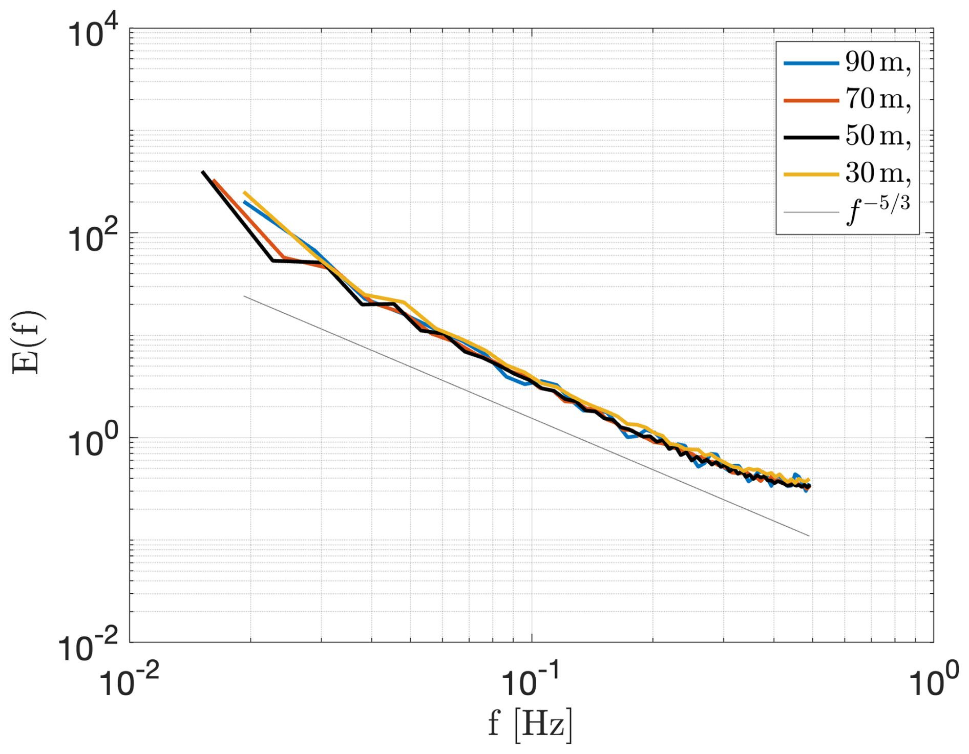
Figure 5 Power spectra E(f) of normalized wind speed u(t) during the T_c periods measured at different heights H. The solid gray line shows a decay $E\left(f\right)\propto f^{-\mathrm{5}/\mathrm{3}}$. The spectra are calculated for each period T_c and then averaged over all periods. A time window of roughly 5 d was considered to extract the definite time series u(t) during T_c>10 s.

4 Comparison to pure turbulent and synthetic wind data

4.1 Experimental wind-tunnel turbulence and IEC standard Gaussian Kaimal

In order to investigate whether the CWS periods are typical features of turbulent flow or are special features of the ABL, we investigate the statistics of the CWS periods T_c from experimental wind-tunnel turbulent data, as well as from synthetic data. The experimental data “Lab” were measured by Renner et al. (2001) in the central region of a free jet, which is approximately stationary, homogeneous, and isotropic. The synthetic data “Kaimal” correspond to IEC standard wind data based on the well-known Kaimal model, with normally distributed amplitudes (Kaimal et al., 1972). The Kaimal data are generated by the National Renewable Energy Laboratory (NREL) TurbSim package (Jonkman, 2016). Details about the parameters and characteristics of the two additional data sets, Lab and Kaimal, are given in Appendix E.

The analysis of the CWS periods from FINO and Kaimal can be easily compared, as the wind data sets u(t) have comparable IEC standard characteristics in terms of mean wind speed, standard deviation, sampling frequency, and integral length scale. However, such a match of parameters to atmospheric data is not possible with the experimental Lab data. To work out the intrinsic features of the periods of CWS from these different data, we used two different approaches to normalize the calculated T_c.

Firstly, the normalization is done by T_c,max, analogous to that in Figs. 3 and 4. The resulting normalized PDFs p(T_c) for the three wind data sets, FINO, Kaimal, and Lab, are shown in Fig. 6. For its interpretation, it is important to remark that the number of data points given by the sampling rate and measured time determines the lowest probability that can be resolved within the PDF. Accordingly, the minimum value of p(T_c) for Kaimal data in Fig. 6 is explained by the smaller amount of data in the sample. Oppositely, the high probability p(T_c) of shorter periods for Lab data is explained by a much higher sampling of the data.

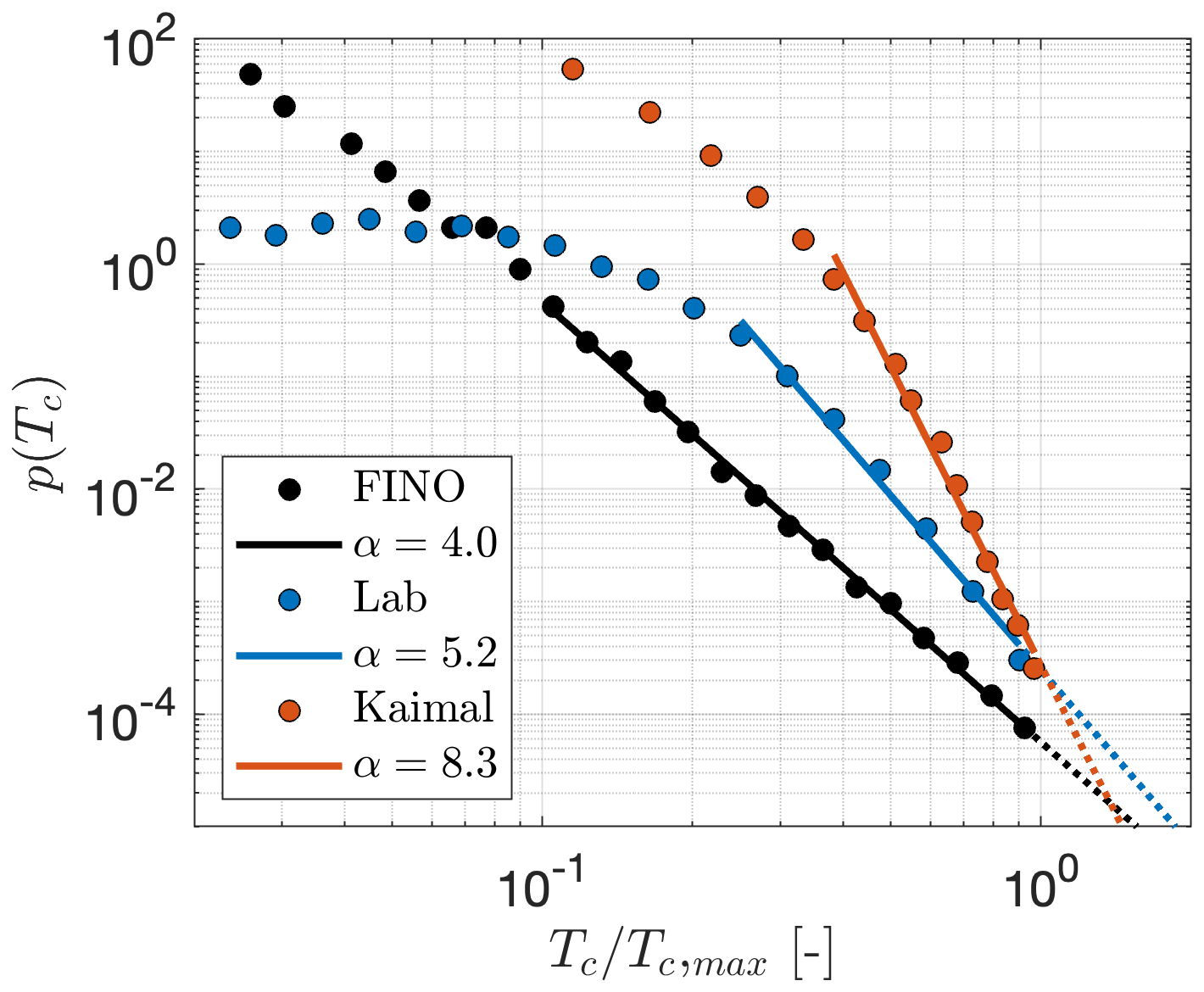
Figure 6 Normalized probability density functions $p(T_{\mathrm{c}}/T_{\mathrm{c},\max })$ for the FINO, Kaimal, and Lab data sets. The power law fittings $\propto T_{\mathrm{c}}^{-\mathit{\alpha }}$ are depicted by the solid lines. The value T_c,max for each data set is defined after a binning process as the center of a bin containing at least 10 of the longest periods measured. Measurements at H=90 m are considered for FINO. The threshold ε=A σ_u for the CSR is calculated with A=0.3. The values of σ_u for Kaimal and Lab are 0.58 and 0.38 m s⁻¹, respectively. In this particular case, as both data sets are expected to be steady, the standard deviation σ_u is calculated over the length of the time series.

Clearly different PDFs are observed for the three data sets in Fig. 6. The most prominent power law $p\left(T_{\mathrm{c}}\right)\propto T_{\mathrm{c}}^{-\mathit{\alpha }}$ is found for the FINO data, with a smaller exponent α or more heavy-tailed probabilities. For the Kaimal and Lab data, a power law is questionable. We nevertheless show power laws as a reference for comparison between the three data sets. Interestingly, the range of periods T_c for which the power law holds for the FINO data extends over a decade, at least from $T_{\mathrm{c}}=\mathrm{0.1}{T}_{\mathrm{c},\max }$ to $T_{\mathrm{c}}=T_{\mathrm{c},\max }$. In contrast, the power law range for Kaimal and Lab spreads only from $T_{\mathrm{c}}=\mathrm{0.3}{T}_{\mathrm{c},\max }$ to $T_{\mathrm{c}}=T_{\mathrm{c},\max }$.

The normalization by T_c,max shown in Fig. 6 does not provide any information regarding the magnitude of the CWS periods T_c. Therefore, a comparison of absolute values T_c between the three data sets remains inconclusive. Accordingly, we chose a second approach to normalize the CWS periods so that their lengths are related to the intrinsic lengths of the flow. The integral length scale L_int is a measure of the longest correlations. For ideal turbulence, structures that are significantly larger than L_int are not to be expected. For meteorological wind data, the problem arises that at lower frequencies, no white noise (i.e., zero correlation) is present, so larger structures than L_int are expected (Sim et al., 2023; Larsén et al., 2016). Thus, we now normalize the periods T_c by the large-eddy-turnover time $T_{\mathrm{int}}=L_{\mathrm{int}}/\stackrel{\mathrm{‾}}{u}$ (Monin and Yaglom, 2007), where $\stackrel{\mathrm{‾}}{u}$ is calculated over the full time series for Kaimal and Lab data. The resulting PDFs p(T_c) after the second normalization approach are shown in Fig. 7.

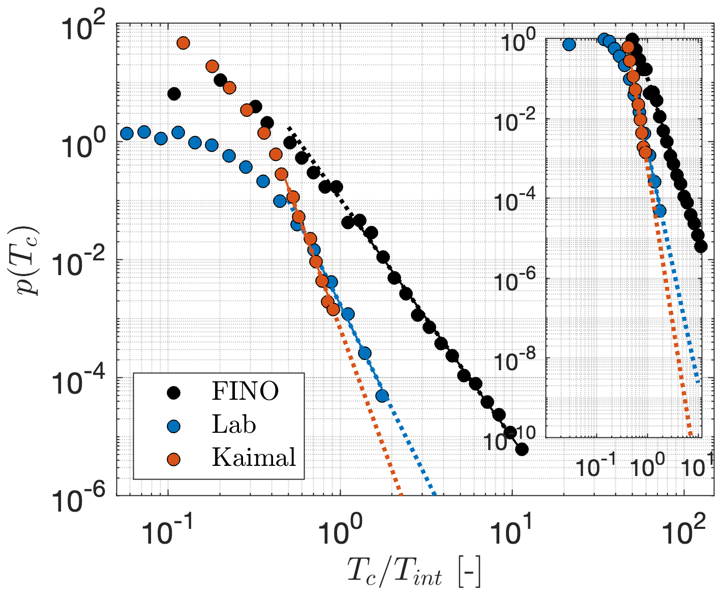
Figure 7 Normalized $p(T_{\mathrm{c}}/T_{\mathrm{int}})$ probability density functions for the FINO, Kaimal, and Lab data sets. The values of T_int are 17 and 0.029 s for Kaimal and Lab, respectively (Fuchs et al., 2022). For FINO, T_int is set to 10 s, as a representative value of the atmospheric data. The power law fittings $\propto T_{\mathrm{c}}^{-\mathit{\alpha }}$ are depicted by the solid lines. The dotted lines show the power law fittings extended over a range of T_c larger than the range used for calculating the fitting parameters.

Figure 7 shows that the FINO data have significantly longer CWS periods T_c. It is observed that the maximal CWS event of the data from the Gaussian Kaimal model, T_c≈ T_int, is around 100 times more frequent for the FINO data than for the other two data sets. Assuming the extended power law tails for Kaimal and Lab depicted by the dotted lines and better visualized in the zoomed plot, a period T_c≈10 T_int would be around 10⁴ times less probable in the Kaimal and Lab data compared to the measured FINO data. From the 1-year FINO data, we measured 15 events T_c≈10 T_int (with $p\left(T_{\mathrm{c}}\right)=\mathrm{5.7}\times {\mathrm{10}}^{-\mathrm{6}}$). It means that there was an observation T_c≈10 T_int roughly every 24 d. Under the IEC Kaimal Gaussian assumption, this event will appear once every 66×10⁴ d or 1808 years.

Furthermore, we calculate the standard deviation of the periods ${\mathit{\sigma }}_{T_{\mathrm{c}}}$ in units of integral lengths L_int. The resulting values are ${\mathit{\sigma }}_{T_{\mathrm{c}},\mathrm{Lab}}=\mathrm{0.12}{L}_{\mathrm{int}}$, ${\mathit{\sigma }}_{T_{\mathrm{c}},\mathrm{Kaimal}}=\mathrm{0.09}{L}_{\mathrm{int}}$, and ${\mathit{\sigma }}_{T_{\mathrm{c}},\mathrm{FINO}}=\mathrm{0.31}{L}_{\mathrm{int}}$. The estimated values of ${\mathit{\sigma }}_{T_{\mathrm{c}}}$ show in another way that FINO data tend to have remarkably longer periods compared to Kaimal and Lab data.

4.2 CTRW wind model

We have shown the results of the distributions of CWS periods p(T_c) in the ABL and their underestimation by the IEC standard Gaussian Kaimal wind model. Consequently, we finally show how the observed features of the atmospheric turbulent data can be included in a numeric wind field model. As a surrogate for the IEC standard Kaimal model, we investigate non-standard wind velocity time series generated by the continuous-time random walk (CTRW) model (Kleinhans, 2008; Ehrich, 2022; Schwarz et al., 2019; Mücke et al., 2011). The CTRW model generates either Gaussian CTRW-G ( with G as an abbreviation for Gaussian) or non-Gaussian CTRW-NG ( with NG as the abbreviation for non-Gaussian) wind velocity time series. For the CTRW-G, the statistics of u(t) are entirely Gaussian. On the contrary, the statistics of u(t) for the CTRW-NG deviate from Gaussianity towards distributions with heavy tails or higher probabilities of rare or extreme events.

The CTRW model is based on a skewed Lévy-distributed stochastic process parameterized by the characteristic exponent α_L. The stochastic process defines a time transformation from the intrinsic scale of the model s to the physical time t. Such time-scaling transformation allows the generation of non-Gaussian time series u(t). The characteristic exponent α_L, with 0 $<{\mathit{\alpha }}_{\mathrm{L}}\le \mathrm{1}$, specifies the asymptotic behavior of the skewed Lévy distribution. For α_L = 1, the resulting process u(t) is entirely Gaussian. Values of α_L→0 generate processes with more pronounced non-Gaussian characteristics. In this case, non-Gaussianity is related to extremely long waiting times between two successive time steps s. A very long waiting time in u(s) would then be translated into a period over which the process u(t) remains constant.

Figure 8 shows an excerpt of u(t) for the Gaussian CTRW-G and non-Gaussian CTRW-NG realizations. Values of α_L=1 and α_L=0.9 are considered for CTRW-G and CTRW-NG, respectively. Along the interval between t=875 and t=895 s, a period of almost constant wind speed is observed for the CTRW-NG. For better visualization, a zoomed version of the time series is presented in the sub-panel in the bottom-right corner. Such a structure of the wind, indicated by the horizontal blue line, agrees with our definition of a CWS period T_c. The small fluctuations observed within the CWS period result from the interpolation process between the intrinsic and the physical times s→t (Ehrich, 2022).

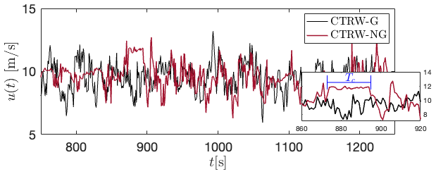
Figure 8 Excerpt of the wind speed time series u(t) for CTRW-G and CTRW-NG. A CWS period T_c is visible between 875 and 895 s in the CTRW-NG. The exponent for the Lévy distribution of the CTRW-NG is α_L=0.9.

The fundamentals of the CTRW model as well as further details on the method for achieving such non-Gaussian features are given in Appendix F. The parameters for generating the time series are provided in Appendix E.

Figure 9a shows the PDFs p(T_c) for the CTRW realizations and the FINO data. The individual distributions are vertically shifted for better visualization. The dotted lines show the Gaussian distributions, with the mean and standard deviation of the corresponding p(T_c). The gray-shadowed area illustrates the range of the decay of p(T_c) or slopes α enclosed by CTRW-G (triangles) with α_L=1 and CTRW-NG (squares) with α_L=0.9. The distribution of the CTRW-NG realization shows an overestimation compared to the FINO data; there is a deviation from Gaussianity towards a higher probability of very long periods of T_c. This deviation is visible in $T_{\mathrm{c}}\approx \mathrm{0.3}{T}_{\mathrm{c},\max }$. On the contrary, the decay of the CTRW-G is much more pronounced, and the divergence from the Gaussian distribution is visible only for events $T_{\mathrm{c}}>\mathrm{0.6}{T}_{\mathrm{c},\max }$. A third realization, CTRW-NG^* (black circles), with α_L=0.995 is included. The resulting p(T_c) distribution for CTRW-NG^* shows better agreement with the FINO data. Both distributions, FINO and CTRW-NG^*, lie inside the gray-shadowed area depicting the slopes enclosed between the Gaussian CTRW-G and extremely non-Gaussian CTRW-NG.

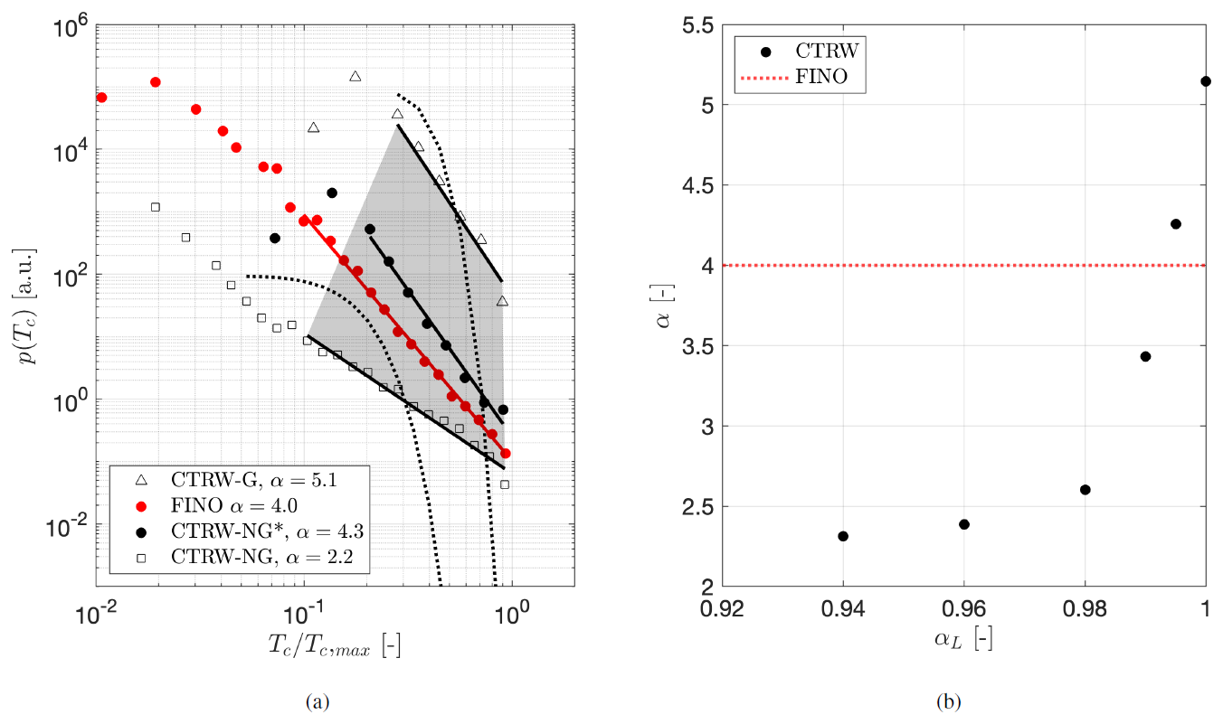
Figure 9 (a) Normalized probability density functions $p(T_{\mathrm{c}}/T_{\mathrm{c},\max })$ for the CTRW-G, CTRW-NG, and CTRW-NG^* and for the FINO data. The gray area depicts the range of the slopes covered between CTRW-G and CTRW-NG. Measurements at H=90 m are considered for FINO. The individual distributions are shifted vertically for better visualization. Dotted lines depict Gaussian distributions. (b) Power law exponents α from $p\left(T_{\mathrm{c}}\right)\propto T_{\mathrm{c}}^{-\mathit{\alpha }}$ as a function of the characteristic exponent α_L from the Lévy distribution of the CTRW model. The horizontal red line depicts the value of α for the FINO data shown in (a).

Figure 9b shows the resulting exponents α from the decay $p\left(T_{\mathrm{c}}\right)\propto T_{\mathrm{c}}^{-\mathit{\alpha }}$ versus the exponent α_L from the Lévy distribution of the CTRW model. The dotted horizontal line depicts the value of α for FINO in Fig. 9a. As observed, by tuning the α_L parameter of the CTRW model, non-Gaussian realizations of u(t) can reproduce the statistics of p(T_c) from turbulent wind in the ABL. Since the resulting distributions p(T_c) are quite sensitive to the Lévy exponent α_L, a careful selection of the exponent is required.

5 Conclusions and outlook

We present measurements of the CWS periods (T_c) (periods with turbulence of a reduced amplitude) from offshore wind data within the ABL. It is shown that the probability distributions p(T_c) for offshore data exhibit a power law decay $p\left(T_{\mathrm{c}}\right)\propto T_{\mathrm{c}}^{-\mathit{\alpha }}$ for very long events (i.e., hundreds of seconds). This agrees with Moreno et al. (2022), where preliminary results from onshore cases were reported. However, significant differences in the values of the exponent α between offshore and onshore conditions suggest that the lengths of T_c are indeed influenced by interactions with the surroundings. Therefore, the estimated statistics of T_c must be considered locally for the specific location of interest. Given that offshore conditions maintain a more unperturbed ABL compared to those onshore, we demonstrated that the periods T_c are intrinsic features of the ABL rather than structures resulting from specific external factors (i.e., mountains, obstacles). Moreover, the exponent α seems to be quite independent of the height but changes significantly with the threshold ε. Less pronounced decays of p(T_c) are obtained with wider thresholds when considering the wind speed to be constant. We found examples of T_c significantly larger than 100 s, which correspond to spatially extended structures over sizes larger than 1 km, using Taylor's hypothesis of frozen turbulence. Such large structures in turbulent wind may be related to the current hot topic of “turbulent superstructures” (Pandey et al., 2018; Krug et al., 2020; Käufer et al., 2023).

Based on the spectral properties, we proved the turbulent nature of the wind speed u(t) during the CWS periods T_c. This relates our results to the case of the turbulent–turbulent interfaces (Kankanwadi and Buxton, 2022). However, the statistics of T_c deviate significantly when comparing different turbulent data. Results from experimental homogeneous isotropic turbulence data suggest that the nature of the periods T_c is attributed to special structures developing in the wind inside the ABL. It is still an open question whether they are caused by special effects of the small-scale turbulence (such as turbulence with or without shear) or whether they are indeed consequences of larger-scale interactions of the atmospheric boundary layer, such as phenomena related to the spectral gap (Larsén et al., 2016).

The frequency of very long events T_c in the ABL is significantly underestimated by the Gaussian assumptions in the IEC models. Therefore, the need for an improved wind model is justified. The continuous-time random walk (CTRW) model, with its characteristic time mapping (see Appendix F), is particularly suitable for the incorporation of the periods T_c measured in the turbulent atmospheric wind. By tuning the exponent of the intrinsic Lévy distribution, different statistics of very long CWS periods can be obtained. This surrogate wind model represents an improvement towards more realistic atmospheric wind fields for numerical simulations. Consequently, results of the WT on the wind when interacting with such disregarded structures might be better predicted.

From an engineering perspective, very long CWS periods might be undesirable for the operation of WTs if phenomena such as resonance or critical loading are induced. On the other hand, they also might be beneficial if conditions such as constant power production are achieved. Further research is needed on the detailed effects of CWS periods on loads by investigating specific WT models.

A very long CWS period might have an increased impact on a WT depending on its spatial location in the plane of the rotor. The effect of such an event happening in the outer region of the rotor plane might be higher compared to the case when it reaches the turbine at the region near the hub. Accordingly, preliminary investigations (detailed in Appendix G) suggest that the periods of CWS show a tendency to be localized at different measurement heights and, therefore, may become of particular interest for turbines with larger diameters. Future work has to be devoted to assessing the relevance of the empirically observed power law behavior of periods of CWS on turbine loading. For that, the complete statistical parameterization of periods of CWS, in both the temporal and spatial domains, should be assessed and improved for the synthetic wind field models such as the proposed CTRW model (Kleinhans, 2008); the recently introduced time-mapped Mann model (Yassin et al., 2023), which can generate long waiting times of u(t) as in the CTRW model; or the super-statistical model (Friedrich et al., 2021, 2022) that follows the K62 model of turbulence. Another interesting aspect for future work would be the statistical analysis of CWS periods from weather-modeled data (e.g., the European Center for Medium-Range Weather Forecasts (ECMWF) and Weather Research and Forecasting (WRF) models). The results would reveal whether such larger-scale models can reproduce the CWS structures within atmospheric forecasting.

Appendix A: CWS periods vs. persistence events

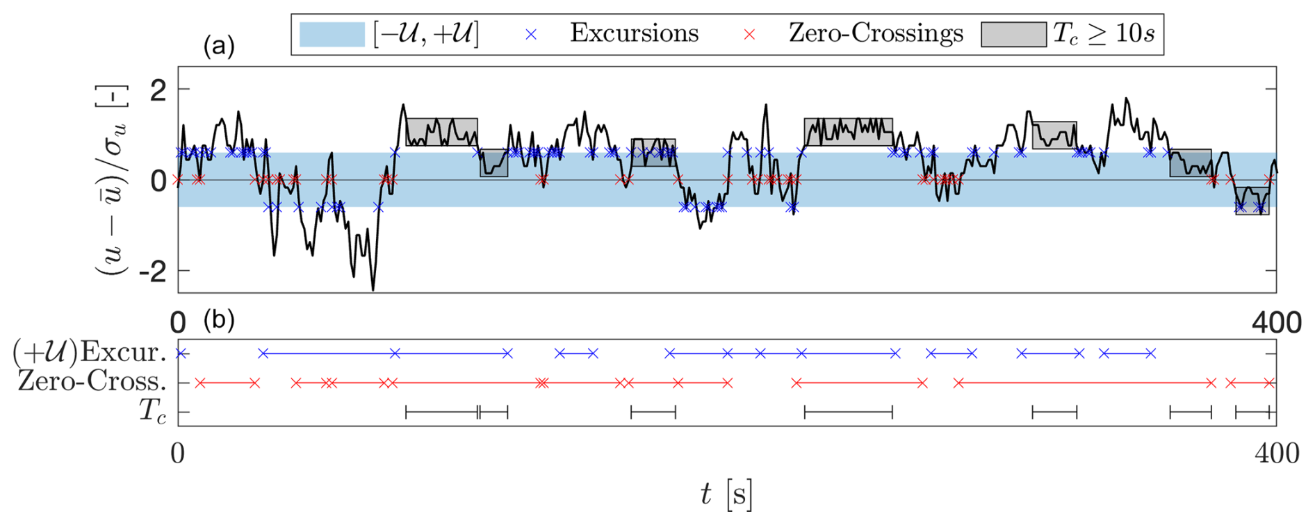
Figure A1 Illustration of excursions, zero crossings, and CWS periods (T_c). Panel (a) is a normalized signal $\left(u\right(t)-\stackrel{\mathrm{‾}}{u})/{\mathit{\sigma }}_u$. The blue crosses depict the excursions, considering ±𝒰 as thresholds. The red crosses correspond to the zero crossings. The gray rectangles mark periods of CWS T_c>10 s. The blue and red lines in (b) depict a selection of the resulting inter-arrival times for the excursion measured at the upper limit +𝒰 and the zero crossings, respectively. Only the inter-arrival periods longer than 10 s are shown. For comparison, the periods T_c>10 s are re-plotted as black lines.

In the Introduction (Sect. 1), we referred to the inter-arrival times of excursions and zero crossings as two general turbulent characteristics within the context of persistence phenomena. Those inter-arrival times might wrongly be assumed to be intrinsically related to our periods of CWS. As shown in Fig. A1, fundamental differences arise when comparing the three events within a turbulent signal. In Fig. A1, a zero-mean and normalized-by-standard-deviation signal $\left(u\right(t)-\stackrel{\mathrm{‾}}{u})/{\mathit{\sigma }}_u$ is plotted. The thresholds ±𝒰 are fixed for considering the excursions of the signal. The blue area depicts the range contained inside these thresholds. The excursion events are depicted by blue crosses. Similarly, the zero crossings are depicted by red crosses. The gray rectangles depict the measured CWS periods T_c>10 s. We assume ε=0.3 for measuring T_c.

In Fig. A1, the length of selected inter-arrival times between the excursion and zero-crossing events and the periods T_c are plotted. The lines follow the color code in panel (a). The selected inter-arrival times are only those longer than 10 s, as was assumed for the periods T_c. As an additional criterion for the excursions (blue lines), only inter-arrival times between successive excursions at the upper limit +𝒰 are considered (i.e., events at −𝒰 are neglected). Note that if all the inter-arrival times were plotted without any distinction, then the individual blue and red lines would overlap, covering the entire length of the time series.

As observed, there is no direct correlation between the occurrence or the length of the CWS periods and the inter-arrival times, neither between excursions nor between zero crossings. A CWS period might enclose several inter-arrival times, and several CWS structures might be embedded inside an interval between consecutive zero crossings or excursions.

Appendix B: Power law distributions

A general quantity x with a probability distribution p(x) follows a power law if

$$\begin{array}{}\text{(B1)}& p\left(x\right)=C{x}^{-\mathit{\alpha }}\end{array}$$

for x≥x_min, with the characteristic exponent α and a constant C=e^c. The minimum value x_min holds for the lowest limit of the power law. The exponent α>1, otherwise ${\int }_{\mathrm{0}}^{\mathrm{\infty }}{x}^{k}p\left(x\right)$, does not converge. The estimation of α from empirical data has been extensively discussed in the analysis of the distributions of a very wide range of applications (Newman, 2005; Clauset et al., 2009). Since Eq. (B1) is equivalent to $\ln p\left(x\right)=-\mathit{\alpha }\ln x+c$, the most simple approach for the calculation of α comes from a linear regression on the log–log plot of the histogram of x. However, this procedure introduces significant errors due to the binning of the data and the resulting distributions. Such distributions are usually dominated by a few bins at lower values of x with very high values of p(x) and several bins in the higher range of x with very low probabilities of p(x) (Newman, 2005; Dorval, 2008). Instead of such a linear regression, a logarithmic binning process of the data is recommended. Within this approach, the histogram of x is constructed for k number of bins with variable widths. More specifically, the bin edges B are proportional to successive powers of a constant a. Then,

$$\begin{array}{}\text{(B2)}& B=(b_{\mathrm{1}},b_{\mathrm{2}},\mathrm{\dots },b_{k+\mathrm{1}})=x_{\mathrm{c},\min }(a^{\mathrm{0}},a^{\mathrm{1}},\mathrm{\dots },a^k),\end{array}$$

where b₁>0, k>1, and x_min is the minimum value of x to consider the power law behavior. Thus, the ith bin encloses the interval $[b_i,b_{i+\mathrm{1}})$, and the larger edge of the kth is assumed to be +∞.

The value of the lower bound x_min affects the estimation of the exponent α in $p\left(x\right)\propto x^{-\mathit{\alpha }}$. Analogously, for binned data, b_min is defined as the minimum bin taken into consideration for the calculation of α. We follow the algorithm proposed by Clauset et al. (2009) and Virkar and Clauset (2014) to choose b_min from binned empirical data. This method is based on a Kolmogorov–Smirnov (KS) statistic test (Massey, 1951) to minimize the distance between the distributions of the fitted model $P\left(b\right|\mathit{\alpha },b_{\min })$ and the empirical model S(b) above b_min. Then, the optimized value of $b_{\min }^{*}$ minimizes

$$\begin{array}{}\text{(B3)}& D={\text{max}}_{b\ge b_{\min }}\left|S\right(b)-P(b|\mathit{\alpha },b_{\min })|.\end{array}$$

Further details about the method for calculating b_min and α are provided in Appendix D.

Appendix C: Statistical moments of power laws

A power law distribution of a continuous variable x is defined in Eq. (B1), where α>1 is the power law exponent, C is a normalization constant, and x_min is the minimum value at which the power law holds. Then, the kth statistical moment of a power law distribution $p\left(x\right)=C{x}^{-\mathit{\alpha }}$ is given by

$$\begin{array}{}\text{(C1)}& \begin{array}{rl}& \langle x^k\rangle =\underset{\mathrm{0}}{\overset{\mathrm{\infty }}{\int }}{x}^{k}p\left(x\right)\mathrm{d}x=\underset{:=\stackrel{\mathrm{̃}}{A}}{\underbrace{\underset{\mathrm{0}}{\overset{x_{\min }}{\int }}{x}^{k}p\left(x\right)\mathrm{d}x}}\\ & +\underset{x_{\min }}{\overset{\mathrm{\infty }}{\int }}{x}^{k}p\left(x\right)\mathrm{d}x=\stackrel{\mathrm{̃}}{A}+{\displaystyle \frac{C}{k+\mathrm{1}-\mathit{\alpha }}}{\left[x^{-\mathit{\alpha }+k+\mathrm{1}}\right]}_{x_{\min }}^{\mathrm{\infty }}.\end{array}\end{array}$$

Then, a quantity x with $p\left(x\right)\propto x^{-\mathit{\alpha }}$ may have divergent moments. Its general kth moment exists only if $k<\mathit{\alpha }-\mathrm{1}$. The mean value of p(x) or 〈x¹〉 becomes infinite for α≤2. Furthermore, if α≤3, p(x) has no finite variance, 〈x²〉. In such a case, x can take values of $\stackrel{\mathrm{‾}}{x}\pm \mathrm{\infty }$. Many phenomena, varying from biological to economical, are characterized by such critical distributions. A few examples are the frequency of the use of words, the income among individuals, and the magnitude of earthquakes (Newman, 2005; Marquet et al., 2005; Powers, 1998).

Appendix D: Estimation of b_min

Here we describe the method introduced in Appendix B for estimating the minimum bin b_min, above which the power law $p\left(T_{\mathrm{c}}\right)\propto T_{\mathrm{c}}^{-\mathit{\alpha }}$ is valid. The method was proposed by Virkar and Clauset (2014).

For each possible $b_{\min }\in (b_{\mathrm{1}},b_{\mathrm{2}},\mathrm{\dots },b_{k/\mathrm{2}})$, we

1. calculate the cumulative binned empirical distribution S(b) for bins b≥b_min,

2. estimate the characteristic exponent $\stackrel{\mathrm{̃}}{\mathit{\alpha }}$ considering b≥b_min,

3. calculate the cumulative density function (CDF) for $P\left(b\right|\stackrel{\mathrm{̃}}{\mathit{\alpha }},b_{\min })$ of the binned power law,

4. calculate the Kolmogorov–Smirnov (KS) test statistic D defined in Eq. (B3), and

5. select the optimal value $b_{\min }^{*}$ as the value of b_min with the minimum test statistic D.

The bins b are defined according to Eq. (B2). For the estimation of $\stackrel{\mathrm{̃}}{\mathit{\alpha }}$ in step (2), a least-squares linear regression method is considered.

Appendix E: Further details of experimental wind-tunnel and synthetic IEC standard wind data

• Kaimal. The data set contains 4×10⁵ data points with a frequency of 1 Hz. The implementation of the Kaimal spectrum for the longitudinal component u of the wind in TurbSim (Jonkman, 2016) follows

  $$\begin{array}{}\text{(E1)}& S_u={\displaystyle \frac{\mathrm{4}{\mathit{\sigma }}_u^{\mathrm{2}}{L}_u/{\stackrel{\mathrm{‾}}{u}}_{\mathrm{H}}}{(\mathrm{1}+\mathrm{6}f{L}_u/{\stackrel{\mathrm{‾}}{u}}_{\mathrm{H}}{)}^{\mathrm{5}/\mathrm{3}}}},\end{array}$$

  where σ_u is the standard deviation, ${\stackrel{\mathrm{‾}}{u}}_{\mathrm{H}}$ is the mean at the hub height, and f is the frequency. The integral scale L_u is defined as L_u=8.10Λ_u, with Λ_u being the turbulence scale. Λ_u is calculated as ${\mathrm{\Lambda }}_u=\mathrm{0.7}\left(\text{min}\mathit{\right\{}\mathrm{30}\text{m},H_{\mathrm{H}}\mathit{\left\}}\right)$, where H_H is the hub height. The parameters are chosen to be comparable to the averaged values of FINO data (see Sect. 2.2). We assume a hub height of H_H=90 m, a mean wind speed ${\stackrel{\mathrm{‾}}{u}}_{\mathrm{H}}$ of 10 m s⁻¹, and a standard deviation σ_u of 0.58 m s⁻¹. Then, the integral length scale is set to 170 m.

• CTRW. Both realizations, CTRW-G and CTRW-NG, have 4×10⁵ data points, with a frequency of 1 Hz. The mean wind speed and standard deviation are 9.5 and 1.1 m s⁻¹ for both cases. Extended parameters for the model are ω_c=1.8 Hz, ${\mathit{\alpha }}_{\mathrm{L}}=[\mathrm{0.9},\mathrm{1}]$, and $\stackrel{\mathrm{̃}}{c}=\mathrm{350}$. Details about the definition of the parameters are given in Appendix F and by Ehrich (2022). The values of the parameters are chosen to generate data comparable to FINO measurements (see Sect. 2.2).

• Lab. The velocity in the direction of the flow was measured by a hot-wire anemometer. The data set consists of 8.48×10⁶ data points, with a sampling frequency of 8 kHz. The measured integral length scale is reported as 0.067 m (Fuchs et al., 2022). Details of the experiment are found in Renner et al. (2001).

Appendix F: CTRW model for the generation of wind fields

More detailed descriptions of the model are provided by Kleinhans (2008), Yassin et al. (2023), Mücke et al. (2011), and Schwarz et al. (2019). Time series of the wind speed $u_i^{\left(\mathit{\kappa }\right)}\left(t\right)$ at each point i of a defined grid are based on two coupled Ornstein–Uhlenbeck (OU) stochastic processes, $u_r^{\mathit{\kappa }}\left(s\right)$ and $u_i^{\mathit{\kappa }}\left(s\right)$. Both processes are first generated in an intrinsic scale s. The super index κ accounts for the three directions of the wind $\mathit{\kappa }=[x,y,z]$. In our case, we generate wind speed time series only in the longitudinal direction u^(x) such that κ=(x). The two processes are defined as

$$\begin{array}{}\text{(F1)}& {\displaystyle \frac{\mathrm{d}{u}_r^{\left(\mathit{\kappa }\right)}\left(s\right)}{\mathrm{d}s}}=-{\mathit{\gamma }}_r\left(u_r^{\left(\mathit{\kappa }\right)}\right(s)-u_{\mathrm{0}}^{\left(\mathit{\kappa }\right)})+\sqrt{D_r}{\mathrm{\Gamma }}_r^{\left(\mathit{\kappa }\right)}\left(s\right)\end{array}$$

and

$$\begin{array}{}\text{(F2)}& {\displaystyle \frac{\mathrm{d}{u}_i^{\left(\mathit{\kappa }\right)}\left(s\right)}{\mathrm{d}s}}=-\mathit{\gamma }\left(u_i^{\left(\mathit{\kappa }\right)}\right(s)-u_r^{\left(\mathit{\kappa }\right)}(s\left)\right)+\sqrt{D_i^{\left(\mathit{\kappa }\right)}}{\mathrm{\Gamma }}^{\left(\mathit{\kappa }\right)}\left(s\right),\end{array}$$

where γ and γ_r are damping constants, D and D_r are diffusion constants, and Γ(s) and Γ_r(s) are Gaussian-distributed white noise. Next, the resulting Gaussian velocity signals $u_i^{\left(\mathit{\kappa }\right)}\left(s\right)$ are mapped to the physical timescale t by means of an additional stochastic process as

$$\begin{array}{}\text{(F3)}& {\displaystyle \frac{\mathrm{d}t\left(s\right)}{\mathrm{d}s}}={\mathit{\tau }}_{\stackrel{\mathrm{̃}}{\mathrm{c}},{\mathit{\alpha }}_{\mathrm{L}}}\left(s\right).\end{array}$$

where ${\mathit{\tau }}_{\stackrel{\mathrm{̃}}{c},{\mathit{\alpha }}_{\mathrm{L}}}\left(s\right)$ is a Lévy-distributed process with a characteristic exponent α_L and a cutoff value $\stackrel{\mathrm{̃}}{c}$. In the case of α_L=1, the intrinsic scale s is equivalent to the physical time t such that $u_i^{\left(\mathit{\kappa }\right)}\left(s\right)$ = $u_i^{\left(\mathit{\kappa }\right)}\left(t\right)$. The time-mapping process described in Eq. (F3) allows the key feature of the model, which accounts for the intermittent behavior of the wind speed time series. The intermittency is introduced by the Lévy-distributed sizes of the waiting times for the transformation from s to t.

In Sect. 4, we investigated two CTRW data sets: CTRW-G and CTRW-NG. For the CTRW-G time series shown in Figs. 8 and 9a, the Lévy exponent α_L is equal to 1 such that the waiting times of the intrinsic scale s are constant and the statistics of u(t) are Gaussian. For the CTRW-NG time series, we assumed α_L=0.9. By doing so, we introduce non-Gaussian features into the probability distributions. Further values of the parameters for generating the fields are given in Appendix E.

Appendix G: Spatial coherence of T_c

The spatial coherence of the CWS periods has been preliminarily investigated. Figure G1 shows the results of evaluating the simultaneity of events T_c>T_min occurring at different heights of the FINO data and conditioned on a reference height $\stackrel{\mathrm{̃}}{H}$. As an example, Fig. G1 shows the case when considering the reference height $\stackrel{\mathrm{̃}}{H}=\mathrm{90}$m and T_min=30 s. Then, for each event T_c>30 s at 90 m, the occurrence of simultaneous events T_c at the remaining heights H is evaluated. A black line is drawn when an event T_c is measured at the corresponding H.

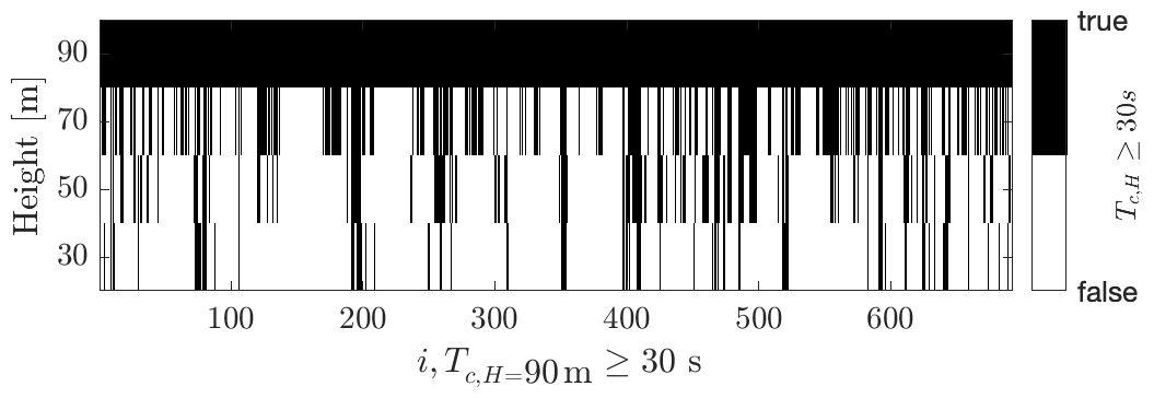
Figure G1 Events T_c>T_min at different heights, conditioned on $\stackrel{\mathrm{̃}}{H}=\mathrm{90}$m. First, the reference height $\stackrel{\mathrm{̃}}{H}$ is defined. Next, for each i event $T_{\mathrm{c},i}>T_{\min }$ at $H=\stackrel{\mathrm{̃}}{H}$, the occurrence of T_c at the remaining heights $H=[\mathrm{70},\mathrm{50},\mathrm{30}]$m is evaluated. Black lines depict the occurrence of an event. The T_c at all heights H is conditioned so that T_c>T_min. For the example in this figure, T_min=30 s and $\stackrel{\mathrm{̃}}{H}=\mathrm{90}$m.

The results show that most of the events are not coherent over the four heights H and confirm the appearance of localized structures. In fact, for the example shown, 37 % of the events at H=90 m are happening simultaneously at H=70 m. This number decreases to 11 % when comparing the CWS periods between H=90 m and H=30 m. The same evaluation for coherent events has been performed for different values of T_min and reference heights $\stackrel{\mathrm{̃}}{H}$.