Observations of wind farm wake recovery at an operating wind farm

The interplay of momentum surrounding wind farms significantly influences wake recovery, affecting the speed at which wakes return to their freestream velocities. Under stable atmospheric conditions, wind farm wakes can extend over considerable distances, leading to sustained vertical momentum flux downstream, with variations observed throughout the diurnal cycle. Particularly in regions such as the US Great Plains, stable conditions can induce low-level jets (LLJs), impacting wind farm performance and power output. This study examines the implications of wake recovery using long-term observations of vertical momentum flux profiles across diverse atmospheric conditions. In these observations, several key findings were observed, such as (a) LLJ heights being altered downstream of a wind farm, especially when the LLJs are below 250 m above ground level; (b) a notable impact of LLJ height on wake recovery being observed using momentum flux profiles at upwind and downwind locations, wherein LLJs between 250 and 500 m above ground level resulted in larger momentum transfer within the wake (i.e., smaller velocity deficit) compared to LLJs below 250 m above ground level; (c) the largest momentum flux variability being observed during stable atmospheric conditions, with non-negligible variability observed during neutral and unstable atmospheric conditions; (d) detection of wake effects almost always being observed throughout the atmospheric boundary layer height; and finally (e) enhancement of wake recovery being observed in the presence of propagating gravity waves. These insights deepen our understanding of the intricate dynamics governing wake recovery in wind farms, advancing efforts to model and predict their behavior across varying atmospheric contexts. In addition, the performance of large-eddy-simulation-based semi-empirical internal boundary layer height model estimates incorporating real-world atmospheric and turbine inputs was evaluated using observations during LLJ conditions.

1 Introduction

Wind turbine wakes, i.e., velocity deficits due to extraction of the kinetic energy from an operating wind turbine, are observed to extend several kilometers during stable atmospheric conditions both onshore and offshore (Hirth et al., 2012; Banta et al., 2015; Krishnamurthy et al., 2017; Fernando et al., 2019; Ahsbahs et al., 2020; Zhan et al., 2020). Wind farm wakes from a large cluster of wind turbines in mesoscale model simulations, and offshore observations can reach over 50 km downwind under stable atmospheric conditions (Platis et al., 2018; Lundquist et al., 2019, Schneemann et al., 2020). Large-eddy simulations of large wind farms also show that wind farm wakes can alter the surface momentum and heat fluxes (Calaf et al., 2011). Wind farm wakes are known to impact the local meteorological conditions by, for instance, increasing or decreasing the temperature and enhancing turbulence downwind of a wind farm (Baidya Roy et al., 2004; Smith et al., 2013; Siedersleben et al., 2018; Miller and Keith, 2018, Bodini et al., 2021), although the intensity of the impact depends on atmospheric stability, local atmospheric processes, orientation of the wind farms, downwind distance, and the number and operative regimes of wind turbines.

In operational wind farms, intra-farm wakes can result in significant power losses, and it is important to understand the dissipation of wakes within a wind farm. The effect of a wind turbine is to decrease the mean velocity and increase the turbulent kinetic energy above the rotor layer (the layer from the bottom of the wind turbine blade tip to the top of the blade tip; VerHulst and Meneveau, 2014). The turbulent transport term in a steady-state filtered-energy equation includes the entrainment of the mean momentum due to turbulence and the entrainment of the turbulent kinetic energy due to fluctuating velocities (Allaerts and Meyers, 2017). Downwind of a wind farm, the recovery of a wind turbine wake within the rotor layer largely occurs due to enhanced entrainment of the vertical momentum flux from the boundary layer (Abkar and Porté-Agel, 2013; Yang et al., 2014; VerHulst and Meneveau, 2014; Abkar and Porté-Agel, 2014; Lu and Porté-Agel, 2015). The maximum energy produced by a large (>100 MW) land-based wind farm is then constrained by the momentum flux between the surrounding atmosphere and the flow within the wind farm. Therefore, measuring the entrainment of the mean momentum due to turbulence upwind and downwind of an operational wind farm can provide insight into the momentum balance of wakes within a wind farm. The momentum balance can be a function of various locally observed atmospheric phenomena, such as low-level jets (LLJs), gravity waves, and high shear or veer events. Atmospheric stability is known to impact the extent of wake propagation downstream (Hansen et al., 2012; Barthelmie et al., 2012; Hirth et al., 2012; Smith et al., 2013; Krishnamurthy et al., 2017; Lundquist et al., 2019). In conjunction with some of the local atmospheric features, the transfer of momentum within and outside the surrounding wind farm can show drastic spatial and temporal heterogeneity.

Today's wind turbines operate within the lowest 300 m of the atmospheric boundary layer (ABL), and in offshore or stable atmospheric conditions the ABL can be lower than 300 m (Shaw et al., 2022). Although wind farms operate within 300 m above ground level, their impacts can be observed through the entire depth of the boundary layer. Therefore, to accurately assess such impacts, observations of mean and turbulent characteristics of wind and temperature should extended up to the top of the ABL. Remote sensing instruments, such as Doppler lidars, are capable of estimating the mean winds within the ABL (Frehlich, 1994, 2001; Peña et al., 2009; Krishnamurthy et al., 2013; Newsom and Krishnamurthy, 2022) as well as turbulence with accuracy comparable to sonic anemometers, which are considered a standard for atmospheric turbulence measurements (Frehlich and Cornman, 2002; Frehlich et al., 2006; Smalikho et al., 2005; Krishnamurthy et al., 2011; Sathe et al., 2015; Bonin et al., 2017; Wildmann et al., 2019). Certain observational studies have validated the propagation of wakes for long distances downwind (more than 20 rotor diameters – RDs) using targeted long-range scanning radar measurements (Hirth et al., 2012; Ahsbahs et al., 2020), satellite-based radar observations (Djath et al., 2018) and airborne observations (Lampert et al., 2020). But other observations have also shown that wake deficits are small at larger RDs (∼26 RD) downstream of a multimegawatt wind farm (Smith et al., 2013). As wake extent grows laterally downwind of a wind farm, measuring velocity deficits at larger downwind distances can get very challenging due to small deficits. Therefore, assessing the impact of wakes purely based on wind speed and turbulence intensity estimates at targeted observational locations would not provide a good representation of wake dissipation. Large-eddy simulations have previously shown momentum deficit estimates within and above the wind farm rotor layer at large downwind distances (Stevens, 2016; Gadde and Stevens, 2021) and provide more realistic information about the influence of wind farm wakes on the atmospheric boundary layer. Therefore, accurately measuring momentum deficits at various downwind distances of a wind farm, rather than just mean winds and turbulence intensity profiles, might provide a better assessment of wind farm wakes. Recent studies have focused on observing momentum flux variability around a wind farm using in situ observations on an aircraft (Syed et al., 2023), but there has not been a study, as per the authors' knowledge, looking at any systematic and statistically significant trends in vertical momentum flux profiles under a variety of atmospheric conditions surrounding an operational wind farm. Therefore, it would be essential to know under what atmospheric conditions wakes recover faster, thereby reducing the impact on downwind wind farms or turbines for optimal siting of wind farms, turbines, and power production estimates.

Gravity waves and atmospheric bores are ubiquitous in the Southern Great Plains (SGP) region (Carbone et al., 1990; Davis et al., 2003; Geerts et al., 2017). Although most frequently observed during nocturnal and stable atmospheric conditions, they vary significantly in their period and amplitude. These nocturnal convective systems typically accompany high winds, intense rain and/or hail, and sometimes tornadoes (Maddox, 1980). The forecast skill of such atmospheric events is relatively low in both numerical weather prediction models and coarse-grid climate models (Davis et al., 2003; Pritchard et al., 2011). They also typically include a LLJ within the atmospheric boundary layer, which supports the moisture transport above the stable boundary layer over the SGP (Berg et al., 2015; Krishnamurthy et al., 2021a). Primarily gravity waves create wave-like oscillations in the atmosphere due to the presence of a density gradient, and bore disturbances are shown to have a significant upward displacement of wind within the troposphere (Rottman and Simpson, 1989; Parsons et al., 2019). Such wave-like disturbances when reaching the surface can create undulations in the mean winds depending on the period and wavelength of the wave. Mountain waves have previously been known to impact the power production of a wind farm (Draxl et al., 2021), but the impact of propagating gravity waves on wake recovery is not very well understood.

Wind farms create a step change in surface roughness, and when the atmospheric boundary layer height (δ) is larger than the surface momentum roughness (z_0 m), an internal boundary layer (δ_IBL) is developed in the region downstream of the surface discontinuity (Elliot 1958; Taylor, 1969; Calaf et al., 2013; Stevens, 2016; Krishnamurthy et al., 2023). The boundary layer flow is observed to adjust to this new surface condition and grows with downstream distance (x). The growth of the internal boundary layer is a function of mean wind, thermal stratification or atmospheric stability, inversion height of the ABL, and surface turbulence characteristics. In the presence of a wind farm, the growth of an internal boundary layer is also a function of the mean wind turbine spacing and characteristics of the wind turbine performance (Calaf et al., 2011; Stevens, 2016; Stevens and Meneveau, 2017). The momentum flux into a wind farm replenishes the wake of the wind farm, and the height of the internal boundary layer can reach up to δ. During stable atmospheric conditions, δ_IBL will grow to reach δ within a short distance from the leading edge of a wind farm, resulting in a fully developed IBL. While most existing studies have been based on high-resolution models, limited long-term observations of δ_IBL growth are available in the literature. Syed et al. (2023) showed spatial variability of momentum flux measurements from in situ sensors on board an aircraft upstream of, above, and downstream of a wind farm but did not provide a vertical profile up to the boundary layer. Therefore, estimating profiles of momentum flux up to the boundary layer depth can provide insights into the impact of internal boundary layers on wind farm dynamics.

Dimensional arguments show that in the far field, i.e., large x, as equilibrium conditions prevail the ratio of the downwind to upwind friction velocity is given as $u_{*}^{\mathrm{d}}/u_{*}^{\mathrm{u}}=F_{\mathrm{1}}(z_{\mathrm{0}}^{\mathrm{u}}/z_{\mathrm{0}}^{\mathrm{d}})$, where $u_{*}^{\mathrm{d}}$ and $z_{\mathrm{0}}^{\mathrm{d}}$ are downwind friction velocity and roughness length, and F₁ is an unknown function, while the superscript u refers to upwind estimates (Krishnamurthy et al., 2023). In the presence of a wind farm, the model presented in Calaf et al. (2011) assumes two constant stress levels, above ($u_{*,\mathrm{hi}}$) and below ($u_{*,\mathrm{lo}}$) the wind turbine, with the difference between those momentum layers given as

$$\begin{array}{}\text{(1)}& u_{*,\mathrm{hi}}^{\mathrm{2}}=u_{*,\mathrm{lo}}^{\mathrm{2}}+{\displaystyle \frac{\mathrm{1}}{\mathrm{2}}}{c}_{ft}{\left(\langle \stackrel{\mathrm{‾}}{u}{\rangle }_{z_{\mathrm{h}}}\right)}^{\mathrm{2}},\end{array}$$

where $\langle \stackrel{\mathrm{‾}}{u}{\rangle }_{z_{\mathrm{h}}}$ is the horizontally and time-averaged velocity at hub height, c_ft= πC_T(4S_xS_y), C_T is the turbine coefficient of thrust, and lateral and transverse spacing between the wind turbines is given by S_x and S_y. Using a logarithmic wind profile formulation ($U\left(z\right)=u_{*}\ln \left(z/z_{\mathrm{0}}\right)/\mathit{\kappa }$), where κ is von Kármán constant (0.4), a relationship for the wind turbine roughness height of the wind farm (z_0,hi) can be estimated (Stevens, 2016). Thereby, the growth of the internal boundary layer due to a wind farm can be estimated using (Willingham et al., 2014)

$$\begin{array}{}\text{(2)}& {\displaystyle \frac{{\mathit{\delta }}_{\mathrm{IBL}}\left(x\right)}{z_{\mathrm{0},\mathrm{hi}}}}={\displaystyle \frac{{\mathit{\delta }}_{\mathrm{IBL}}\left(\mathrm{0}\right)}{z_{\mathrm{0},\mathrm{hi}}}}+C_{\mathrm{1}}{\left({\displaystyle \frac{x}{z_{\mathrm{0},\mathrm{hi}}}}\right)}^{\mathrm{4}/\mathrm{5}},\end{array}$$

where, x is the downwind distance, δ_IBL(0) is the internal boundary layer height of the wind turbine rotor top at the first row of the wind farm (equal to the wind turbine blade upper tip height), z_0,hi is the surface roughness due to the presence of a wind farm, and C₁ is a growth constant (0.28) estimated from large-eddy simulation models (Calaf et al., 2011; Stevens, 2016). The wind farm surface roughness is a function of the upwind surface friction velocity, wind turbine and farm parameters, and inflow mean wind conditions within the wind turbine rotor layer. Existing large-eddy simulation estimates of internal boundary layers have typically used idealized conditions, while estimates in real-world atmospheric conditions of the IBL might differ considerably due to competing atmospheric conditions. Therefore, observations of internal boundary layer growth are important to understand the impact of wind farms on the ABL and thereby the momentum balance surrounding a wind farm and associated wake replenishment.

In this paper we investigate the wake recovery of a wind farm by investigating the momentum balance (primarily mean streamwise momentum flux: $\langle u{}^{\prime }w{}^{\prime }\rangle$) surrounding an operational wind farm near the Atmospheric Radiation Measurement (ARM) program Southern Great Plains (SGP) sites in Oklahoma during various site-specific atmospheric phenomena. Momentum flux profiles from scanning Doppler lidars and surface sonic anemometers are estimated for both upwind and downwind locations relative to the wind farm. Information about the field campaign and site characteristics is given in Sect. 2. Momentum flux profiles upwind and downwind of an operational wind farm during site-specific atmospheric conditions are discussed in Sect. 3. Wind farm IBL measurements and comparison of data with theoretical models are given in Sect. 4, and results are summarized in Sect. 5.

2 Field campaign and site characteristics

Oklahoma ranks third in the United States for installed wind capacity, providing over 37 418 GWh of electricity in 2022. The state generated approximately 44 % of its electricity from wind energy in 2022, the third-highest in the country, and provided enough electricity to power millions of US homes. The landscape and topographic flows around SGP are relatively simple compared to complex-terrain sites with low wind speed interannual variability (<3 %) and therefore are favored by wind farm developers (Krishnamurthy et al., 2021a).

To investigate the interaction between wind farms and the ABL and improve our understanding of wind turbine and wind farm wake effects, the US Department of Energy (DOE) funded a field campaign, the American WAKE experiemeNt (AWAKEN), within and adjacent to King Plains wind farm near Enid, Oklahoma (Debnath et al., 2023; Moriarty et al., 2024). Figure 1 shows the domain of the AWAKEN field experiment, various locations with instruments deployed, and operational wind turbines within the domain. Several remote sensing and in situ sensors were deployed; please see Moriarty et al. (2024) for additional details of the site setup and layout.

In this article, data from primarily two instrumented sites are used for data analysis. Site A2 is the inflow site and site H the outflow site to the King Plains wind farm during southerly wind directions. Figure 1 shows a picture of both the sites and various instruments deployed. Site A2 was instrumented with a scanning Doppler lidar, short-range vertical profiling lidar, surface sonic anemometer, and surface meteorological station, while site H had a scanning Doppler lidar, microwave radiometer, and two disdrometers. Both the scanning lidars were oriented close to north, like the sonic anemometers. Azimuth and elevation offsets for the scanning lidars were identified by using the stationary tower near the wind farm as a hard target. These offsets were used to correct the observed azimuth and elevation angles from the scanning lidars (as described in Newsom and Krishnamurthy, 2022). Frequent hard target scans were conducted to evaluate any drift in the leveling of the lidar, and none was observed during the period of study. The internal pitch and roll of the lidars were constantly below 0.1°. In addition, boundary layer height estimates from a ceilometer at site A1 (also an inflow site) were used to evaluate the impact of boundary layer structure on wind farm wake propagation. The wind turbines deployed at the King Plains wind farm are GE 2.8 MW machines with a hub height of 89 m and a rotor diameter (RD) of 127 m. The average lateral and transverse distance in southerly wind directions between wind turbines (over the eastern sector of the King Plains wind farm, intersecting sites A1 and H) is approximately 3.15 RD (Sx) and 14.57 RD (Sy). Site A2 is approximately 40 RD upwind of the first row of the King Plains wind farm, site A1 is approximately 2 RD upwind, and site H is approximately 22 RD downwind of the last row of the King Plains wind farm. Additional details on various instruments deployed at the AWAKEN site can be found in Moriarty et al. (2024).

Both scanning lidars installed at A2 and H run a composite scan routine that includes 20 min of six-beam profiling (Sathe et al., 2015) and 10 min of vertical stares. Wind profiles from 100 to 3000 m are obtained by applying the well-established least-squares fit to the radial velocity measurement from the six beams (Newsom and Krishnamurthy, 2022). Momentum flux is also estimated through the technique described in Appendix A2 applied to the upstream and downstream beams based on the selected wind direction sector of interest (see Eq. A3). In the following, momentum flux measurements from the surface sonic anemometer at the respective site are also combined with the lidar retrieval to extend the observable range down to the surface. Measurements only from southerly wind directions, specifically from 166 degrees to 190°, are considered in this analysis. Additionally, since removing all outliers from lidar observations is challenging, the median of the sample will be presented in the remainder of the paper.

Figure 2a shows the wind rose at 105 m above ground level from Doppler lidar measurements collected from 17 March to 10 September 2023. Wind directions were predominantly southerly during the duration of the study. Figure 2b shows the distribution of various atmospheric stability conditions as a function of wind direction. Atmospheric conditions were divided into various classes based on the Obukhov length (L) scale as provided in Krishnamurthy et al. (2021a) and Table 1 below. The Obukhov length, L, is given by

$$\begin{array}{}\text{(3)}& L=-{\displaystyle \frac{u_{*}^{\mathrm{3}}T}{\text{kg}\langle w^{\prime }{\mathit{\theta }}_v^{\prime }\rangle }},\end{array}$$

where T is the air temperature, g is the acceleration due to gravity, and $\langle w^{\prime }{\mathit{\theta }}_v^{\prime }\rangle$ is the kinematic heat flux from sonic anemometers.

At SGP C1 (which is ∼21 km north of King Plains wind farm), stable atmospheric conditions were observed more than 50 % of the time. During neutral conditions, a larger percentage of winds were either easterly or northerly. It is important to note that surface atmospheric stability might not always be representative of conditions at elevated levels, especially during transition periods (i.e., during sunset and sunrise).

Table 1 Stability classification based on L thresholds.

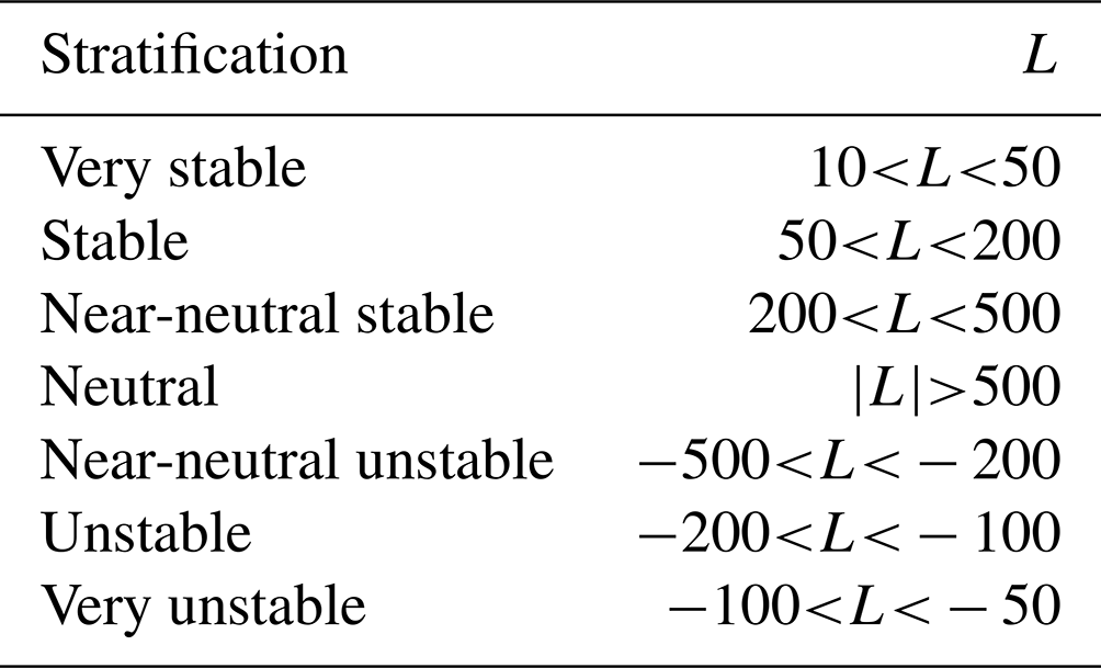
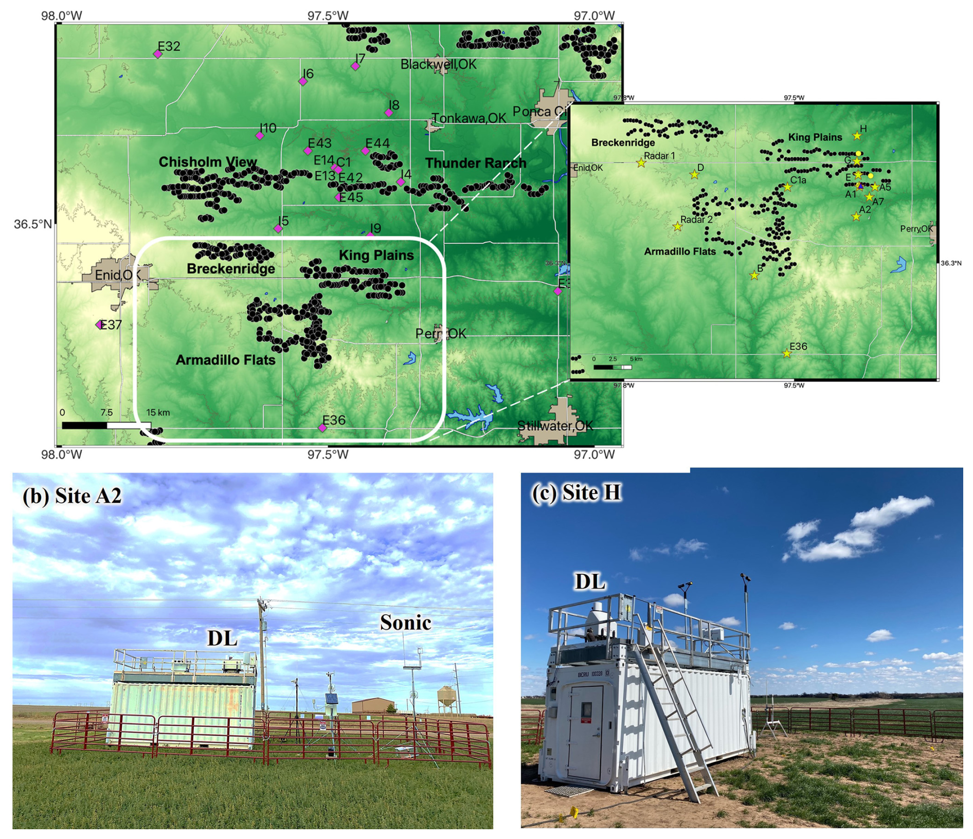
Figure 1 (a) Southern Great Plains area with the location of the AWAKEN field campaign (white box) shown. Various sites deployed (yellow stars and circles) during the AWAKEN field campaign, DOE ARM sites (magenta diamonds), and the wind turbines (black circles) in the area (Moriarty et al., 2024). (b) Images of instruments deployed at site A2 (inflow to King Plains wind farm for dominant southerly wind directions) and (c) site H (downwind of King Plains wind farm) are also shown at the bottom.

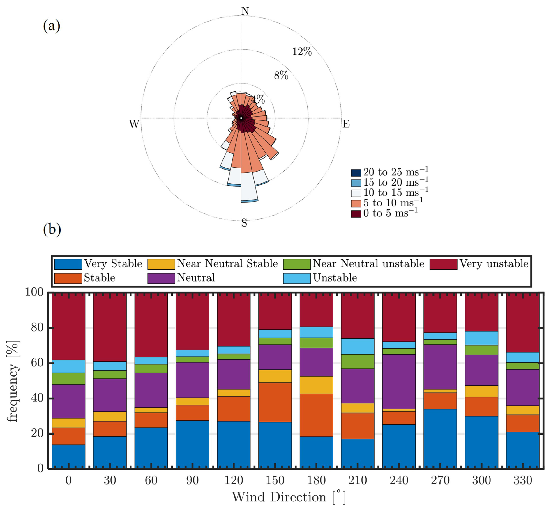
Figure 2 (a) Wind rose at 105 m a.g.l. from a Doppler lidar at the SGP central facility during all atmospheric conditions. (b) Atmospheric stability classification as a function of wind direction from 17 March to 10 September 2023. Various atmospheric stability classes are distinguished based on L and defined in Krishnamurthy et al. (2021a) and Table 1.

3 Wake recovery observations

To minimize the impacts of wakes from neighboring wind farms (including the Breckinridge and Armadillo Flats wind farms shown in Fig. 1) in our analysis and to measure the impact of wakes from at least three rows of wind turbines, measurements only from southerly wind directions, especially from 166 to 190°, are considered. Since the wind directions are predominantly southerly, sufficient data are available (1490 10 min samples) to accurately estimate the mean trends of momentum flux during specific atmospheric conditions. Below, statistics of momentum flux variability under different atmospheric conditions, such as varying levels of thermal stratification (stability), the LLJs, high wind shear and veer conditions, ABL depth, and atmospheric gravity waves, are assessed.

3.1 Impact of atmospheric stability on wake recovery

As shown in Fig. 2b, when winds are southerly the atmospheric stability is predominantly (>50 %) stable near the surface, with neutral conditions occurring about 20 % of the time and unstable conditions observed for the remainder. Figure 3 shows median momentum flux ($\langle u{}^{\prime }w{}^{\prime }\rangle$) profiles from the downwind (site H) and upwind (site A2) locations during stable, neutral, and unstable atmospheric conditions. In general, we observe higher negative momentum flux upwind of the wind farm near the surface with an asymptotic behavior eventually reaching zero near δ, like a canonical atmospheric boundary layer. Downwind of the wind farm, enhanced $\langle u{}^{\prime }w{}^{\prime }\rangle$ is observed due to the shear and turbulence generated by the wind turbines. Stable conditions are observed to show larger deviations in momentum flux downwind of the wind farm compared to neutral or unstable atmospheric conditions. The sign of momentum flux is tied to the vertical wind shear, as for sustenance of turbulence within a wind farm an increase in wind shear (positive) should result in negative momentum flux downwind of the wind farm.

Therefore, in stable atmospheric conditions, due to large (positive) wind shear, the momentum flux must be negative to create downwind turbulence. As mentioned earlier, the wind farm wake propagates longer in stable conditions due to lower ambient turbulence compared to convective conditions. Therefore, at site A2, which is approximately 22 RD downwind of the last row of the King Plains wind farm, the region of enhanced vertical momentum flux due to the wind farm is expected to be more persistent and varies with the diurnal cycle (Fig. 3a). In Fig. 3b and c, larger momentum flux estimates are observed near the surface during unstable and neutral atmospheric conditions compared to stable conditions. Under neutral conditions, where shear is less positive and ambient turbulence is higher compared to stable conditions, the momentum flux generated by downwind wind turbines is anticipated to be lower or less persistent. Consequently, wakes are not expected to travel as far. But in Fig. 3b, significant momentum flux deficits are still observed at 22 RD downwind during neutral conditions. A couple of possible reasons for this could be due to (a) misclassification of atmospheric stability from surface flux measurements, i.e., surface atmospheric stability at hub height is not representative of the true atmospheric state, and (b) higher wind shear observed during neutral conditions resulting in more negative momentum fluxes within the wind farm wake. The larger the vertical momentum flux, the faster the wake velocity recovers to a freestream value (Syed et al., 2023). During unstable atmospheric conditions, wakes are expected to dissipate faster (convective mixing of the atmospheric boundary layer), and due to low wind shear, the momentum flux deficits are expected to be significantly lower. In Fig. 3c, it is evident that during unstable conditions the momentum flux deficits are lower but still observed 22 RD downwind. Overall, momentum flux deficits are greater during unstable conditions at higher altitudes, while they are larger during stable conditions at lower heights. One potential reason for deficits observed during unstable conditions at 22 RD downwind could be the impact of convectional updrafts or downdrafts on the propagation of wake downwind of a wind farm (Berg et al., 2017; Wang et al., 2020). Additional analysis is required, ideally using high-resolution large-eddy simulations, to truly evaluate the impact of updrafts and downdrafts on wind farm wakes. Overall, the median deficit observed over King Plains wind farm shows that the flow disturbance downwind of a wind farm can extend long distances (at least 22 RD) in every atmospheric condition. Such differences are generally not very evident from solely observing wind profile observations upwind and downwind of a wind farm.

As mentioned earlier, no observations of vertical profiles of momentum flux have been recorded to date within an operational wind farm; therefore, there is limited knowledge on the height at which the peak transfer of momentum occurs downwind of a wind farm. It is well known that the peak velocity deficit (upwind – downwind velocity) generally occurs at hub height, but there are no observations showing the peak momentum deficit above the wind farm. Based on large-eddy simulation results, the peak momentum deficit is expected to occur near the upper edge of the wind turbine rotor layer (Abkar and Porté-Agel, 2015), but based on observations at King Plains wind farm, in stable conditions, at 22 RD downwind, peak momentum flux is consistently observed at ∼0.36 RD above the wind farm. Therefore, the mean kinetic energy entrainment height into the wake is observed to occur higher than in traditional large-eddy simulation (LES) models. Additional comparisons between LES models and observations are required to further evaluate the wake recovery processes within the wind farm wake.

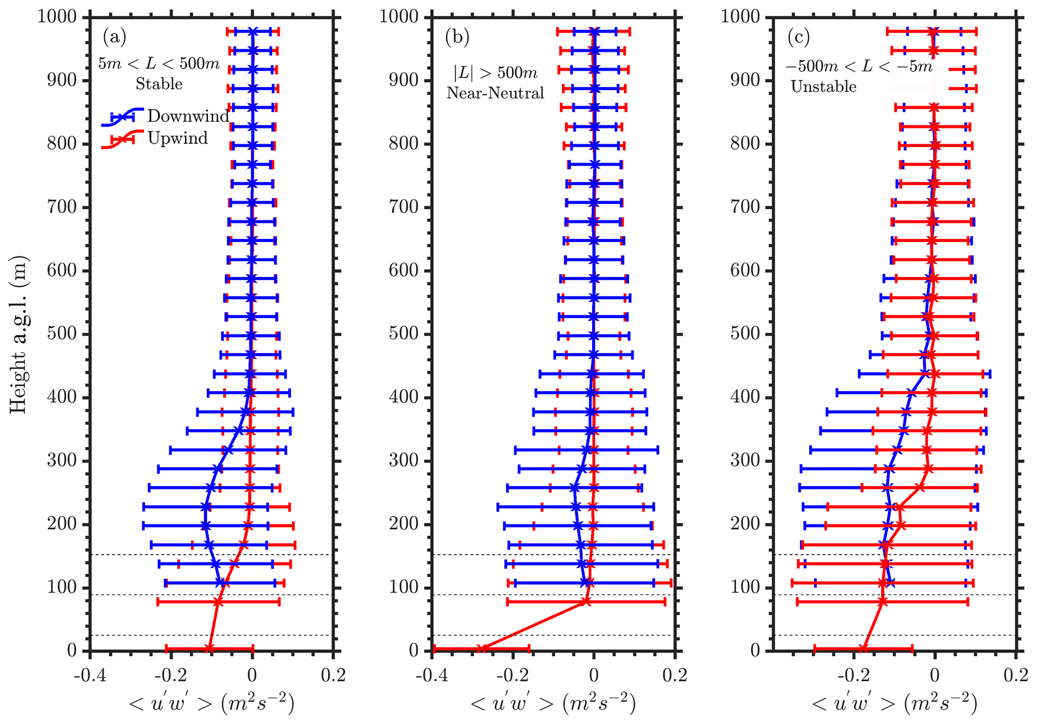
Figure 3 Momentum flux profiles at ∼40 RD upwind (site A2) and 22 RD downwind (site H) of the King Plains wind farm during (a) stable, (b) near-neutral, and (c) unstable atmospheric conditions. The vertical extent of the wind turbine rotor layer is also shown with horizontal dotted black lines. The near-surface Obukhov length (L) is used to differentiate between different stability conditions. Error bars represent the sample standard deviation at respective heights. Measurements only from southerly wind directions, specifically from 166 to 190°, and from 17 March to 10 September 2023 are considered in this analysis.

3.2 Impact of LLJs on wake recovery

Stable conditions produce LLJs in the US Great Plains (Berg et al., 2015; Krishnamurthy et al., 2021a), whose characteristics can modulate wind farm performance and power output (Gadde and Stevens, 2021). There are several definitions of low-level jet height (Z_LLJ) in the literature (Blackadar, 1957; Bonner 1968; Whiteman et al., 1997; Song et al., 2005; Kalverla et al., 2019; Debnath et al., 2023), but in this article it is defined as per Song et al., 2005. The definition is based on two criteria: (1) wind speed maximum (i.e., LLJ nose) is observed within the lowest 2 km and is greater than at least >10 ms⁻¹, and (2) wind speed drop-off above the jet nose is observed and above a set threshold (at a minimum >5 ms⁻¹). Three categories of LLJs were identified based on varying thresholds of drop-off speeds and maximum nose wind speed (Song et al., 2005), although in this analysis all LLJ categories were combined. Figure 4a shows the distribution of various near-surface atmospheric stability classes during southerly wind directions (from 166 to 190°) during LLJ events and associated median Z_LLJ for each atmospheric stability class. It can be observed that lower Z_LLJ values are typically associated with very stable or stable near-surface atmospheric conditions, while higher Z_LLJ values are observed when the surface atmospheric stability is not stable, indicating a decoupled boundary layer (Vanderwende et al., 2015). Therefore, there could be confounding influences of the near-surface stability and LLJ influence on the wind farm wakes during such instances. Figure 4b shows LLJ nose wind speed as a function of median Z_LLJ per wind speed bin and hub-height wind speed, and Fig. 4c shows Z_LLJ as a function of hub-height wind speed. It is evident that, up to near rated wind speed (approximately 13 ms⁻¹), a higher Z_LLJ results in a higher jet nose wind speed and a higher hub-height wind speed. Overall, it is challenging to decipher various processes influencing wind farm wake recovery using observations, but it would be possible to isolate certain common features known to influence wind farm recovery (LLJ height; atmospheric stability, atmospheric boundary layer, or hub-height wind speed) and study the variability observed during such select features.

As previously observed using historical measurements from the ARM SGP site, the Z_LLJ generally falls within 500 m above ground level (Debnath et al., 2023). Since the scanning lidar measurements start from ∼100 m above ground level, in this analysis we only evaluate LLJs observed above the turbine hub height (>110 m). Therefore, the observations are partitioned into two halves: (a) 250 m < Z_LLJ<500 m and (b) 110 m <Z_LLJ<250 m. The partitioning was driven by selecting a height near the wind turbine rotor layer (25.5 to 152.5 m) that could be impacted by the wind turbine, considering the frequency of LLJ events from southerly wind directions (which peaked around 250 m above ground level) and the observed peak in momentum flux during stable conditions, which occurred approximately 250 m above ground level as shown in Fig. 3. Figure 5 shows vertical profiles of momentum flux and wind speed both upwind and downwind of the wind farm for different Z_LLJs as mentioned above and further conditioned to only southerly wind directions (166 to 190°). During southerly LLJ events at the King Plains wind farm, it is observed that the transfer of momentum into the wake of the wind farm is a function of the LLJ height. Higher Z_LLJ is associated with larger momentum transfer within the wake and lower velocity deficit at 22 RD downwind. In short, the wake recovery is faster when the LLJ height is higher. This is mainly due to the shear-generated turbulence below the Z_LLJ and the enhanced momentum deficit developed due to the wind farm. The peak entrainment height is observed to marginally increase with higher Z_LLJ. These results support some of the hypotheses from previous LES model results on this topic (Gadde and Stevens, 2021). One unique feature that is observed when 127 m <Z_LLJ<250 m is that the Z_LLJ is influenced by the presence of the wind farm. Downwind (22 RD) of the farm, the Z_LLJ is consistently observed above the wind farm. The downwind Z_LLJ is approximately equal to the height of the internal boundary layer (δ_IBL) generated due to the presence of the wind farm. In addition, during LLJ conditions, Z_LLJ is typically assumed to be the top of the atmospheric boundary layer (δ, Liu and Liang, 2010), as the turbulence above the Z_LLJ is negligible. Figure 6 shows a schematic of the interaction between the wind farm, varying Z_LLJs, and growth of the internal boundary layer due to the presence of the wind farm. Figure 7 illustrates the probability distribution of LLJ events at the upwind site (A2) and downwind site (H) of the King Plains wind farm. The data reveal that the difference in LLJ height between the upwind and downwind sites is greater below approximately 250 to 300 m but diminishes at higher LLJ heights. Notably, there is a reduced frequency of LLJs observed downwind of the wind farm when LLJs occur below the rotor layer. Future research will focus on further analyzing the effects of LLJs that occur beneath the turbine rotor layer.

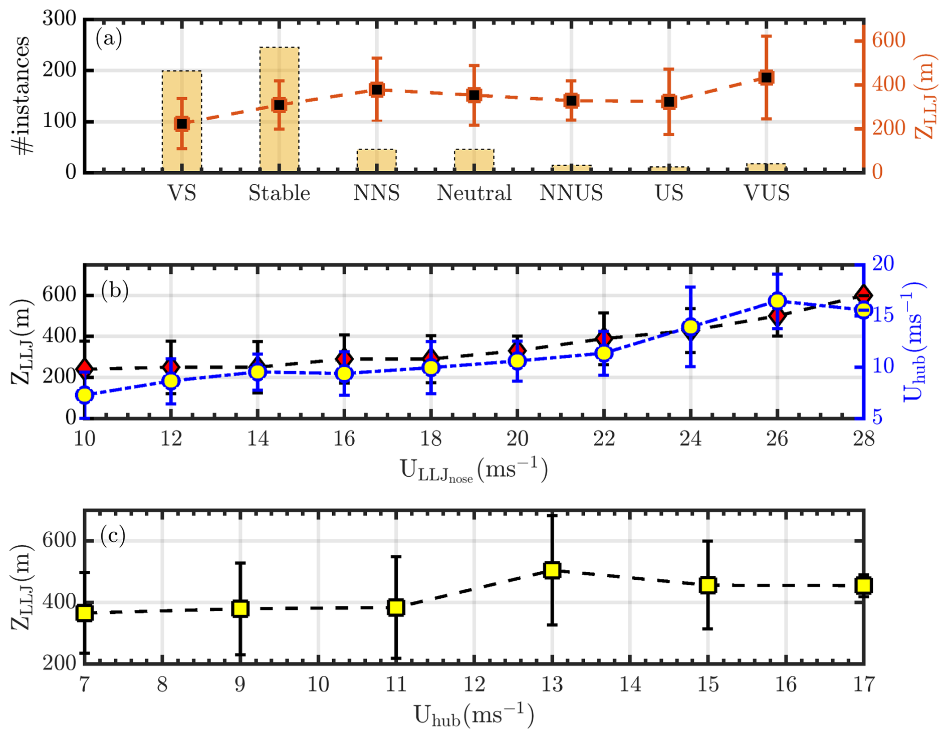
Figure 4 (a) Distribution of various atmospheric stability classes (VS – very stable, stable, NNS – near-neutral stable, neutral, NNUS – near-neutral unstable, US – unstable, VUS – very unstable, as per Sathe et al., 2015) during LLJ events from southerly wind directions and associated Z_LLJ per stability class. (b) Median LLJ nose wind speed (U_LLJnose) as a function of Z_LLJ and hub-height wind speed (U_hub) at the upwind site (site A2). (c) Z_LLJ as a function of U_hub. The error bars indicate 1 standard deviation. Minimum Z_LLJ is 110 m and maximum Z_LLJ is 690 m a.g.l. Measurements only from southerly wind directions, especially from 166 to 190°, and from 17 March to 10 September 2023 are considered in this analysis.

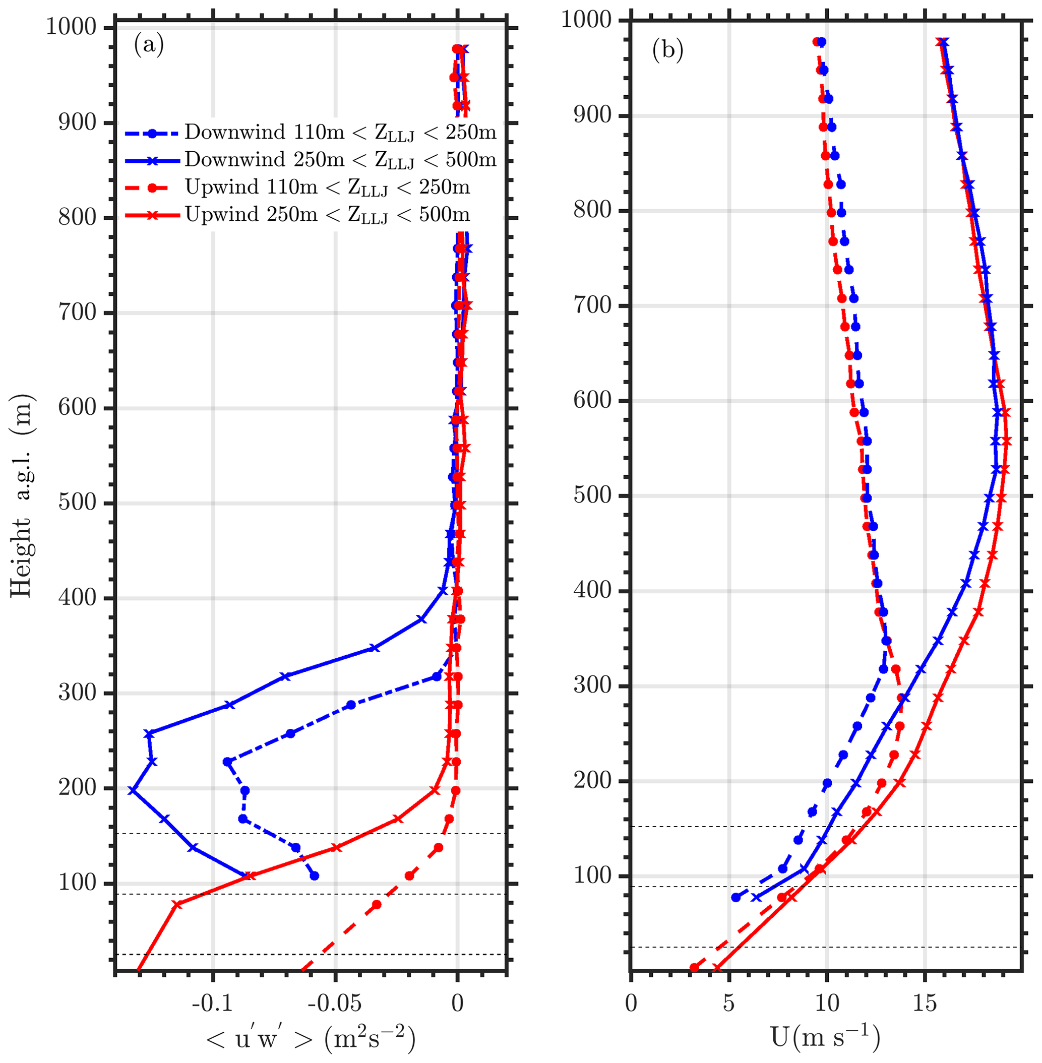
Figure 5 (a) Momentum flux and (b) horizontal wind speed profiles upwind (red, site A2) and downwind (blue, site H) of the King Plains wind farm during conditions when the Z_LLJ is less than 250 m a.g.l. at the upwind location (dash-dotted) and Z_LLJ is between 250 and 500 m a.g.l. (star dotted). The vertical extent of the wind turbine rotor layer is also shown with horizontal dotted black lines. Measurements only from southerly wind directions, especially from 166 to 190°, and from 17 March to 10 September 2023 are considered in this analysis.

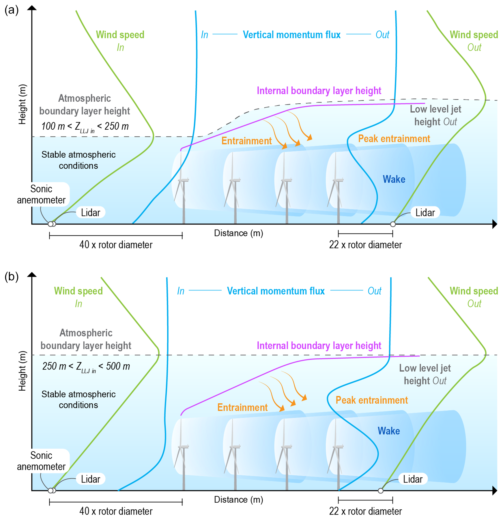
Figure 6 Schematic of the impact of LLJs on a wind farm boundary layer when (a) 100 m <Z_LLJ<250 m and (b) 250 m <Z_LLJ<500 m.

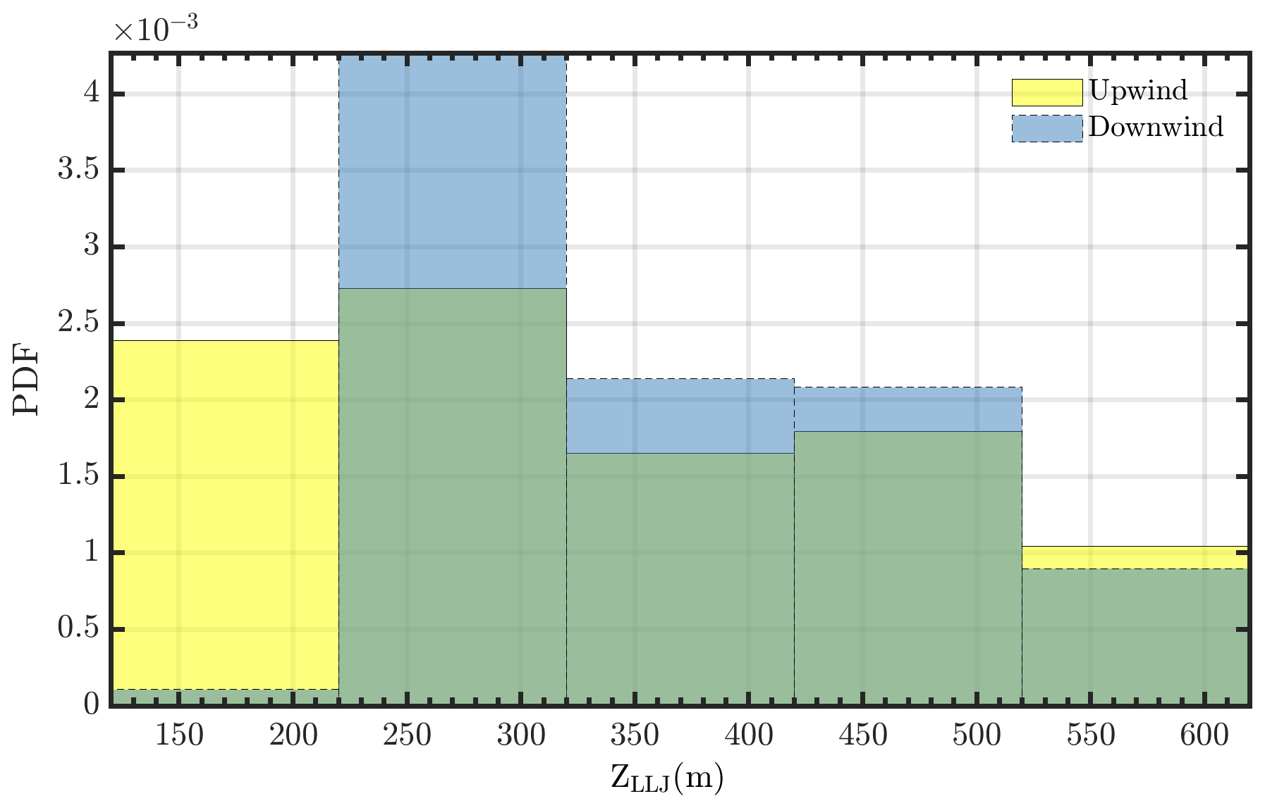
Figure 7 Probability distribution of LLJ heights (Z_LLJ) upwind (site A2, yellow bar graph) and downwind (site H, blue bar graph) of the King Plains wind farm during southerly wind directions.

3.3 Impact during varying shear and veer (non-LLJ) conditions on wake recovery

High wind shear and veer conditions are generally observed within a wind farm, but it is difficult to decouple the effects of shear or veer conditions compared to atmospheric stability conditions. Nonetheless, it would be helpful to observe any consistent trends during such conditions as they are known to impact the power production of a wind farm (Murphy et al., 2020). In addition, such findings may be informative for wind farm control concepts that yaw wind turbines away from the predominant wind direction at hub height but do not currently consider the wind veer within the rotor layer (Fleming et al., 2019). Figures 8 and 9 show median profiles of momentum flux and horizontal wind speed both upwind and downwind of the King Plains wind farm during non-LLJ events for various shear and veer conditions, respectively. Estimates associated with positive and negative wind shear or veer conditions during southerly wind directions are provided.

Hub-height wind speed (U(H)) and shear exponent (α) are estimated by fitting a power-law vertical wind profile to the wind speed data available within the rotor layer (here from 90 to 153 m due to lack of observations below 90 m). The power-law fit is conveniently recast into a linear fit through a log transformation as shown in Eq. (4) below:

$$\begin{array}{}\text{(4)}& \log U\left(z\right)=\log U\left(H\right)+\mathit{\alpha }\log \left({\displaystyle \frac{z}{H}}\right),\end{array}$$

where $\log \left(\frac{z}{H}\right)$ and log U(z)  are the independent and dependent variables of the linear fit, respectively. Hub-height wind direction (ϕ(H)) and veer ($\mathit{\beta }\equiv \frac{\partial \mathit{\varphi }}{\partial z}$) are estimated in a similar fashion but using a linear wind veer model, as follows:

$$\begin{array}{}\text{(5)}& \mathit{\varphi }\left(z\right)=\mathit{\varphi }\left(H\right)+\mathit{\beta }(z-H).\end{array}$$

This approach for estimating hub-height quantities has the advantage of leveraging all the available measurements while mitigating possible biases due to the lack of data in the lowest half of the rotor layer.

Certain trends are immediately observed for cases with positive or negative shear conditions (Fig. 8), where, regardless of the wind shear profile, momentum deficits generated due to the wind farm are observed 22 RD downwind of the wind farm. But both wind and momentum deficits are higher during conditions with high wind shear (0.5<α<2) compared to low or negative wind shear (α≤0) cases, although a lower number of cases were recorded when the wind shear was low or negative at the King Plains wind farm compared to high wind shear cases. Median wind speeds at hub height during both conditions are ∼5 ms⁻¹. For cases with negative wind shear, the median wind speed differences between upwind and downwind are negligible, but a clear trend in median momentum flux profiles is observed. Traditionally it is expected for the wind speed to reach approximately 99 % of the freestream wind speed, but in cases such as this where the wind speeds do reach near freestream, it could be erroneously assumed that the wind farm wake has completely been dissipated (Djath and Schulz-Stellenfleth, 2019). In reality, added turbulence due to the presence of a wind farm is not completely removed downwind of a wind farm under such circumstances. Additional research is needed to evaluate wind farm wake models or parameterization schemes during such canonical atmospheric conditions.

During cases with positive (β>0.1° m⁻¹) and negative (β<−0.1° m⁻¹) wind veer conditions, median wind speeds are closer to the cut-in wind speeds of the GE 2.8 MW wind turbines, and therefore no momentum flux deficits are observed (Fig. 9). Both high and low wind veer cases show that the median wind speeds are relatively low at King Plains wind farm. It is noted that the wind farm has also been observed to modify the wind direction downwind of a wind farm (not shown).

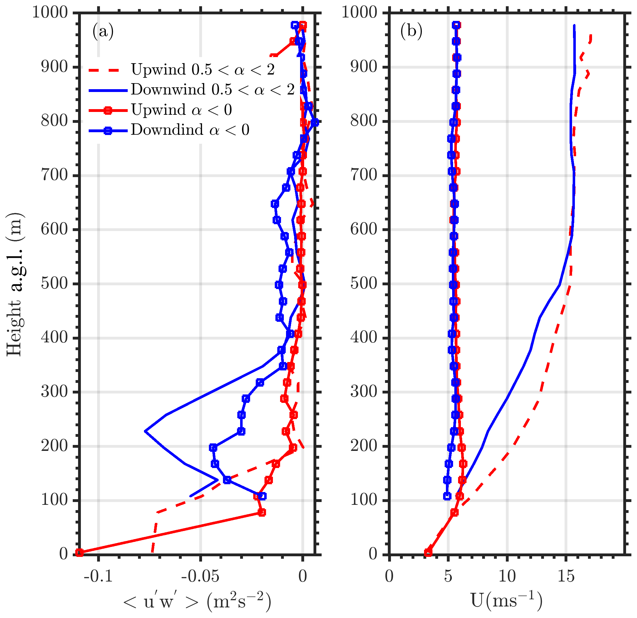
Figure 8 (a) Momentum flux and (b) horizontal wind speed profiles upwind (red) and downwind (blue) of the King Plains wind farm during high (0.5<α<2, observed 53 % of the time) and negative (α≤0, observed 2 % of the time) wind shear conditions. Measurements only from southerly wind directions, especially from 166 to 190°, and from 17 March to 10 September 2023 are considered in this analysis.

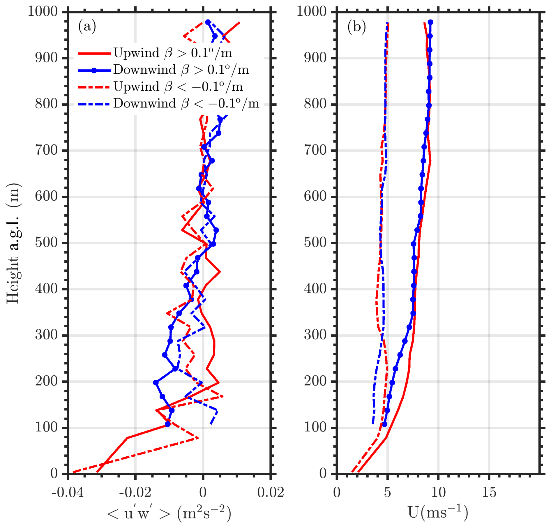
Figure 9 (a) Momentum flux and (b) horizontal wind speed profiles upwind (red) and downwind (blue) of the King Plains wind farm during high (β>0.1° m⁻¹, observed 28.5 % of the time) and negative (β<−0.1° m⁻¹, observed 1 % of the time) wind veer conditions. Measurements only from southerly wind directions, especially from 166 to 190°, and from 17 March to 10 September 2023 are considered in this analysis.

3.4 Extent of wake within the ABL

The atmospheric boundary layer height (δ) is an important parameter for understanding the exchange of momentum, heat, and moisture between the free troposphere and the surface. Unfortunately, estimating δ can be challenging and there is limited consensus on the best approach to estimate δ from remote sensing instruments (Kotthaus et al., 2023). Typically, instruments such as scanning Doppler lidars or ceilometers are used to estimate δ (Tucker et al., 2009; Krishnamurthy et al., 2021b; Zhang et al., 2022). A ceilometer was deployed at the inflow site A1 and is used to estimate δ during southerly wind directions for this evaluation. The boundary layer (or mixing) height, provided by the Vaisala CL-31 BL-View software, is based on three different algorithms: (a) the gradient method (where the algorithm detects the gradient in backscatter profile), (b) the profile method (where the algorithm determines the mixing height by fitting an idealized backscatter profile to the observed range-corrected ceilometer backscatter profiles), and (c) the merged gradient and profile fit method (Zhang et al., 2022). There are several filters applied to the data, such as cloud and precipitation filters, and additional outlier removal techniques (due to instrument noise). Figure 10 shows the median momentum flux and horizontal wind speed profiles during southerly wind directions and measurement co-located when concurrent ceilometer measurements were also available. The median δ (∼540 m) at A1 from the ceilometer is below the height where the median momentum flux estimates at sites A2 and H are nearly equal (∼760 m). Therefore, it is observed that the median ceilometer δ does not accurately predict the height of the atmospheric boundary layer. There are several possible reasons for this; for example, (a) the ceilometer uses the gradient in backscatter aerosol concentrations to estimate δ, which might not always be the top of the boundary layer (Zhang et al., 2022), and (b) upwind and downwind δ might be different due to the presence of the wind farm. Therefore, the δ estimated by the ceilometer represents the δ at the inflow site well (upwind momentum flux is observed to be close to zero). Above δ, the momentum flux deficits due to the presence of the wind farm are negligible. But overall, it is evident that the impact of the wind farms almost always reaches the top of the atmospheric boundary layer. Therefore, it is important to model not only the wind turbine rotor layer with high vertical resolution but also up to δ to accurately assess the impacts of wind farms and wake recovery.

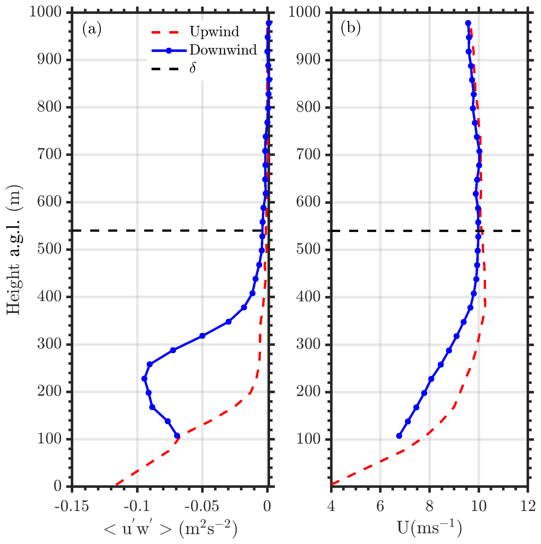
Figure 10 (a) Momentum flux and (b) horizontal wind speed profiles upwind (red) and downwind (blue) of the King Plains wind farm for all atmospheric conditions. The median height of the ABL (δ) from ceilometer measurements is also shown. Measurements only from southerly wind directions, especially from 166 to 190°, are considered in this analysis.

3.5 Impact of a gravity wave event on wake recovery

Figure 11 shows a time–height cross-section of vertical velocity as observed near the ARM SGP central facility Doppler lidar (Newsom and Krishnamurthy, 2022; Krishnamurthy et al., 2021a) on 24 July 2023 from 03:00 to 04:00 UTC (19:00 to 20:00 local time). The vertical velocity clearly shows wave-like features at approximately 800 m a.g.l., where we observe a positive and negative shift in vertical velocity. Figure 12 shows median momentum flux and wind speed both upwind and downwind of the King Plains wind farm on 24 July 2023 from 03:30 to 04:00 UTC. The winds were predominantly southerly during this event, with a veer of 0.0375 ° m⁻¹ from the surface up to the top of the boundary layer. A nocturnal LLJ was also observed at approximately 220 m a.g.l. at the inflow site, and the gravity wave is propagating above the nocturnal stable atmospheric boundary layer (∼Z_LLJ). The peak-to-peak amplitude of the gravity wave is observed to be ∼600 m, which spans from 400 m above ∼1000 m.

As observed in Fig. 12, the momentum flux deficit is significantly enhanced above and within the wake of the King Plains wind farm. Estimates of vertical momentum flux deficits are more than 3 times the median estimates of momentum flux deficits observed during LLJ conditions (see Fig. 5). Downwind, as previously noted, the peak of a LLJ is observed to be displaced significantly above the wind farm, which is a function of the enhanced mixing within the wind farm rotor layer. The higher the mixing, the larger the entrainment and the higher the displacement of the LLJ. Above the LLJ, the gravity wave is observed to have an inverse effect, where the momentum flux is positive, indicating that momentum is transferred upwards to the gravity wave. The positive or negative transfer of momentum near the gravity wave probably depends on the updrafts or downdrafts of the wave, but over the 30 min average observations the overall transfer of momentum is upwards. The negative wind shear above the LLJ could also add to the extraction of momentum from the wind farm. This reduces the intensity of the LLJ and the extracted momentum results in higher wind speeds above the LLJ downwind of the wind farm. It is observed that, in this case, the wind farm has significantly altered the winds not only within the δ but also above it, modulating the shape and intensity of the LLJ. Additional analysis would be needed to see the spatial impact of wind farms during gravity wave propagation and power production. The next steps would be working towards a climatology of gravity waves in the region and its impact on wind farm performance.

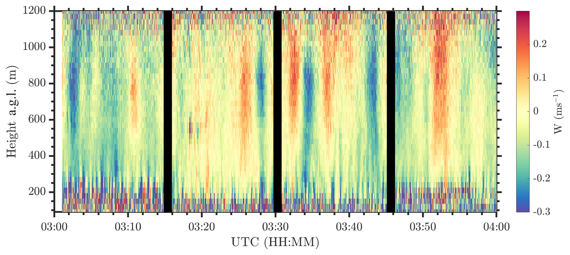
Figure 11 Time–height cross-section of vertical velocity (W) at the ARM SGP central facility on 24 July 2023 from 03:00 to 04:00 UTC. The gaps in data every 15 min are when the lidar performs wind profiles (Newsom and Krishnamurthy, 2022).

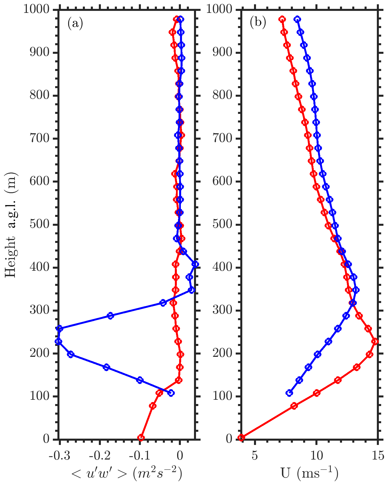
Figure 12 (a) Momentum flux and (b) horizontal wind speed profiles upwind (red) and downwind (blue) of the King Plains wind farm during a gravity wave event on 24 July 2023 at 03:30 UTC.

4 Comparisons of observed δ_IBL with theoretical estimates

As discussed earlier, an internal boundary layer (δ_IBL) is developed due to a step change in surface roughness. Turbulence is expected to be higher within the internal boundary layer (downwind of the surface roughness) compared to inflow (upwind of the surface roughness). Wind farms create a step change in surface roughness and are known to develop internal boundary layers downwind of a wind farm (Calaf et al., 2011; Stevens and Meneveau, 2017). In addition to the roughness impacts of the wind turbines, the wind-farm-developed internal boundary layer is convolved with the wake of the wind turbines, which create additional momentum deficits downwind of the wind farm. Internal boundary layers can be estimated from a velocity profile by identifying a kink in the velocity profile (Garratt, 1990). Although this method provides a general trend, it is known to be not very accurate. An alternative technique, proposed in Stevens (2016), is being implemented here, where the difference in streamwise momentum flux profiles upwind and downwind of a surface roughness change are used to estimate the growth of the internal boundary layer. Vertical momentum flux is responsible for the influx of momentum into the wake of a wind farm. Larger streamwise momentum flux deficits above the wind farm are mainly observed due to turbulence and shear generated by the wind turbines. Wind turbine wakes enhance vertical mixing above a wind farm, which results in a downward flow of momentum. The internal boundary layer height (δ_IBL) is the height when the upwind and downwind momentum flux estimates are approximately within 1 %–5 % of each other above the wind farm.

Wind farm δ_IBL is typically capped by δ, but previous LES modeling results have shown it to penetrate the upwind δ during LLJs (Gadde and Stevens, 2021). As shown earlier, model formulations exist to estimate δ_IBL downwind of a wind farm (Eq. 2). But the growth constant and wind farm surface roughness formulations have been fine-tuned based on large-eddy simulations, and as per the authors' knowledge, no significant analysis of the validation of such formulations has been conducted so far using real-world observations. This article does not attempt to do that comparison in detail but is the start of such comparisons. The model formulations (Eq. 2) are sensitive to surface roughness in the presence of a wind farm (z_0, hi) and the growth constant (C), which can significantly vary δ_IBL estimates within the model (sensitivity analysis not shown for brevity). The model formulations also do not explicitly restrict the growth of δ_IBL but are implicitly treated in models where the sub-grid-scale mixing does not exceed δ, especially during stable atmospheric conditions.

Figure 13 shows the difference in estimates of δ_IBL from observations and model formulations (Eq. 2) only during stable atmospheric conditions and in the presence of a LLJ. Since we have higher confidence in δ_IBL during these cases and δ already represents the top of the LLJ height, this also avoids introducing additional uncertainty from ceilometer δ observations. Some of the inputs to model formulations are provided by real-world observations, such as the lidar 10 min average wind speed at hub height, inflow surface friction velocity and roughness from sonic anemometers, thrust curve of the GE 2.8 MW wind turbine, and average wind turbine spacing in southerly wind directions. Given real-world inputs, the median δ_IBL difference between the model and observations is approximately 50 m; i.e., the model underestimates the δ_IBL. During some extreme cases (Δδ_IBL>200 m) the model does not behave due to inconsistent wind directions for a sustained period (several hours). Additional research is needed with large-eddy simulations or numerical weather prediction models with real-world forcing to assess the recovery and growth of δ_IBL at an operational wind farm.

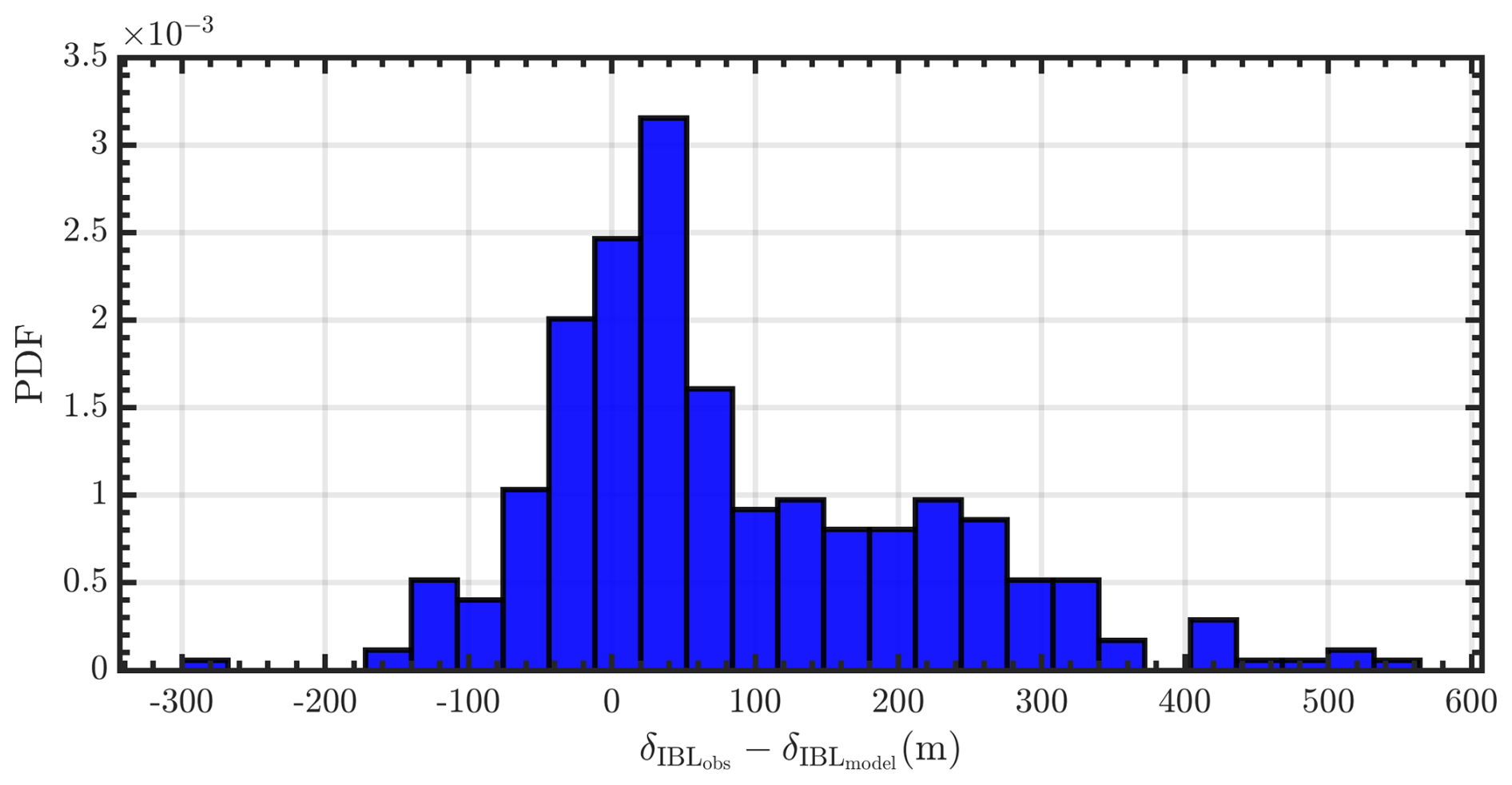
Figure 13 Probability distribution of δ_IBL difference between observations and a semi-empirical model (Eq. 2) during stable atmospheric conditions and in the presence of a LLJ.

5 Conclusions

These novel observations reveal the temporal and spatial variability of momentum balance within and above wind farm wakes during region-specific atmospheric conditions. Profiles also show the growth of the internal boundary layer and allow quantification of the accuracy of current large-eddy-simulation-based approximations in estimating the growth of the internal boundary layer (IBL).

The momentum balance surrounding a wind farm may impact wake recovery. The greater the momentum flux, the faster the wake velocity recovers to a freestream value. Wind farm wakes are known to propagate long distances during stable atmospheric conditions, and thereby the vertical momentum flux added due to the presence of the wind farm is more persistent at downwind locations and varies with the diurnal cycle. Stable conditions also produce LLJs in the US Great Plains, which are known to impact the performance and power output of commercial wind farms. Figure 6 shows a schematic of the impact of varying Z_LLJ on wind farm wake recovery and modulation of the flow downwind of the wind farm. Therefore, long-term measurements of vertical momentum flux upwind and downwind of a wind farm can provide a holistic view of the physical mechanisms behind wake recovery during various atmospheric conditions. In this study, we have evaluated the impact on wake recovery using long-term observations of vertical momentum flux through the boundary layer during a variety of atmospheric conditions. Overall, some highlights of the observations are mentioned below.

1. Wind farms alter LLJ characteristics downwind of the wind farm by elevating the height of the jet above the wind farm (see Figs. 5 and 6).

2. The height of the LLJ significantly impacts wind farm wake recovery downwind, with higher Z_LLJs resulting in faster wake recovery (see Figs. 5 and 6).

3. Negative wind shear during non-LLJ cases show short wake propagation at 22 RD downwind of a wind farm.

4. Wind farm wake impacts are observed through the δ (see Fig. 10).

5. Gravity waves enhance wake recovery and accelerate winds above the LLJ downwind of a wind farm (see Fig. 12).

6. Large-eddy-simulation-based theoretical δ_IBL models show a large spread given real-world inputs of the atmosphere and turbine.

Finally, we have highlighted several areas of research in this article that still need to be explored to understand the dynamics of the wind-farm-influenced atmospheric boundary layer, as mentioned below.

1. Additional comparisons between LES models and observations are required to further evaluate the wake recovery processes within a wind farm wake, since most mesoscale wake model parameterizations are assessed using outputs from LES models.

2. It is important to model not only the wind turbine rotor layer with high vertical resolution but also up to the top of the δ to accurately assess the impacts of wind farms and wake recovery (as shown in Fig. 10), as it is important to understand the entrainment of winds from the ABL to the wind farm wake boundary layer.

3. Long-term (1 year +) evaluation of wind farm wake models or parameterizations using long-term atmospheric flux observations through the boundary layer to assess the true performance of such models is recommended.

4. Analysis would be needed to see the spatial impact of wind farms during gravity wave propagation and power production.

5. Research is needed with large-eddy simulations or numerical weather prediction models with real-world forcing to assess the recovery and growth of δ_IBL at an operational wind farm.

Future work will focus on developing a methodology to classify gravity waves in the region and assess the power production impacts in the presence of gravity waves at the King Plains wind farm site. In addition, comparison of observations and models will be conducted to refine wind farm parameterization schemes within numerical weather models.

Appendix A: Flux estimation algorithms and approach

Herein we provide details of the algorithms used to estimate momentum fluxes from surface-based anemometers and scanning Doppler lidars as well as a methodology to estimate the height of the internal boundary layer from upwind and downwind momentum flux profiles.

A1 Momentum flux estimates from sonic anemometers

Sonic anemometers are considered a standard for estimating atmospheric turbulence parameters (Wilczak et al., 2001, 2019; Fernando et al., 2019). Three-dimensional (3-D) acoustic anemometers provide measurements of winds and temperature at high temporal frequency (>=20 Hz), which supports calculation of higher-order statistics with good accuracy (Cook and Sullivan, 2020). The sign conventions of the 3-D winds vary for different manufacturers and for Gill sonic anemometers, which were deployed for this project; the sign conventions are defined as positive for the upward vertical wind component (w) and upward atmospheric fluxes, the u wind component (north–south) is positive towards north, and the v wind component (east–west) is positive towards the west. The raw and flux data files are generated as per Cook and Sullivan (2020) and contain 30 min of post-processed data and estimates of turbulent fluxes. The sonic data are post-processed by first applying a de-spiking procedure (Goring and Nikora, 2002) to remove any data anomalies, and a two-axis coordinate rotation is performed (Wilczak et al., 2001), which ensures $\langle w\rangle =\langle v\rangle =\mathrm{0}$ and 〈u_s〉=U, where U is the mean wind speed, u_s is the streamwise component, and 〈⋅〉 is a 30 min temporal average. To estimate the fluxes, the average of each variable is estimated over a 30 min (non-overlapping) window, and no detrending of the data is performed to estimate the velocity fluctuations. The stress tensor is then computed using 30 min measurements of velocity fluctuations and assumed to be statistically stationary over the averaging window. Momentum flux estimates from sonic anemometer data were calculated using the eddy-covariance method (Stull, 1988).

A2 Momentum flux profiles from Doppler lidars

A brief description of the method to estimate momentum flux profiles from lidars is given below (Eberhard et al., 1989; Mann et al., 2010). The radial velocity (v_r) equation of a Doppler lidar is given by

$$\begin{array}{}\text{(A1)}& \begin{array}{rl}{v}_{\mathrm{r}}\left(R,\mathit{\theta }\right)& =u\left(R\right)\sin \mathit{\phi }\cos \mathit{\theta }+v\left(R\right)\sin \mathit{\phi }\sin \mathit{\theta }\\ & +w\left(R\right)\cos \mathit{\phi },\end{array}\end{array}$$

where R is the range, φ is the half-opening angle of the conical scan (30°), θ is the azimuthal direction of the lidar beam (0° is north), and u, v, and w are the wind components at each range-gate center. The variance of v_r is given by

$$\begin{array}{}\text{(A2)}& \begin{array}{rl}{\mathit{\sigma }}^{\mathrm{2}}\left[v_{\mathrm{r}}\left(R,\mathit{\theta }\right)\right]& ={\mathit{\sigma }}_u^{\mathrm{2}}{\sin }^{\mathrm{2}}\mathit{\phi }{\cos }^{\mathrm{2}}\mathit{\theta }+{\mathit{\sigma }}_v^{\mathrm{2}}{\sin }^{\mathrm{2}}\mathit{\phi }{\sin }^{\mathrm{2}}\mathit{\theta }\\ & +{\mathit{\sigma }}_w^{\mathrm{2}}{\cos }^{\mathrm{2}}\mathit{\phi }+\mathrm{2}\langle u^{\prime }{v}^{\prime }\rangle {\sin }^{\mathrm{2}}\mathit{\phi }\cos \mathit{\theta }\sin \mathit{\theta }\\ & +\mathrm{2}\langle u^{\prime }{w}^{\prime }\rangle \cos \mathit{\phi }\sin \mathit{\phi }\cos \mathit{\theta }+\mathrm{2}\langle v^{\prime }{w}^{\prime }\rangle \\ & \cos \mathit{\phi }\sin \mathit{\phi }\sin \mathit{\theta },\end{array}\end{array}$$

where u^′, v^′, and w^′ are the velocity fluctuations. One can estimate the streamwise momentum flux components ($\langle u^{\prime }{w}^{\prime }\rangle$) by calculating the radial velocity variance in the upwind and downwind directions over 30 min (Eberhard et al., 1989; Mann et al., 2010), which is then given by

$$\begin{array}{}\text{(A3)}& \langle u^{\prime }{w}^{\prime }\rangle ={\displaystyle \frac{{\mathit{\sigma }}^{\mathrm{2}}\left[v_{\mathrm{r}\mathrm{down}}\right]-{\mathit{\sigma }}^{\mathrm{2}}\left[v_{\mathrm{r}\mathrm{up}}\right]}{\mathrm{2}\sin \mathrm{2}\mathit{\phi }}},\end{array}$$

where σ²[v_r down] and σ²[v_r up] are the radial velocity variances from the nearest downwind and upwind azimuth angles relative to the mean wind direction, respectively. The nearest up and down radial velocities from the azimuth angles are picked for each 30 min sample and given range-gate wind direction estimate. It can be noted from Eq. (A3) that in a positively sheared turbulent flow, σ²(v_r up)> σ²(v_r down), i.e., the upwind variances, are typically larger than downwind variances. The effect of measurement volume is not considered in this analysis and has been shown to have a minimal impact on the streamwise momentum flux measurements for Doppler lidars (Mann et al., 2010).

For evaluating the accuracy of the algorithm, continuous velocity azimuth display (VAD) scans at the same elevation and azimuth angles are required to calculate the variance of the radial velocity along each beam. From 8 October 2020 to 14 January 2021, continuous eight-point planned position indicator (PPI) scans (Δaz=45° and el=60°) were conducted at the Atmospheric Radiation Measurement (ARM) Southern Great Plains (SGP) central facility to support an ongoing field campaign. The mean wind direction (ϕ) at each height is calculated using the approach of Newsom et al. (2017), wherein a chi-square distribution is fit to estimate the horizontal wind vector. Each beam was averaged for 6 s to provide a robust estimate of radial velocity and study the effect of noise from individual radial velocity measurements (Frehlich, 2001). This averaging could underestimate the variance observed by the lidar. During this study, each 360° wind profile was completed in ∼1 min. This provided the ability to calculate the variance of radial velocity along each beam and the momentum flux profile using Eq. (A3). Along-wind momentum flux ($\langle u^{\prime }{w}^{\prime }\rangle$) estimates from the sonic anemometer at 60 m and lidar at 75 m from southerly wind directions are shown in Fig. A1a.

Doppler lidar $\langle u^{\prime }{w}^{\prime }\rangle$ measurements are observed to correlate reasonably well with sonic anemometer $\langle u^{\prime }{w}^{\prime }\rangle$ measurements, with a slope of 0.85 and a coefficient of determination of ∼78 %. During stable atmospheric conditions, given the degree of stratification within the lidar probe volume, the lidar could be measuring very different atmospheric conditions compared to a sonic anemometer. Figure A1b shows measurements from southerly wind directions and very stable atmospheric conditions (10 m <L<150 m). The coefficient of determination is observed to be reduced during stable conditions to ∼63 %, although the wind speeds are observed to correlate well under all conditions. The transfer of momentum is lowest in stable atmospheric conditions and therefore smaller momentum flux estimates are observed. From a purely statistical standpoint, the smaller magnitude of the fluxes also contributes to reducing the coefficient of determination, since under these conditions the contribution of instrumental and statistical noise to the physical variability is relatively larger. The scatter between lidar and sonic measurements is primarily due to (a) 15 m vertical and ∼250 m horizontal separations between sonic anemometer and lidar measurements, (b) low temporal sampling of the lidar measurements, and (c) spatial averaging of the lidar pulse (range gate 30 m). These effects are amplified during stable atmospheric conditions and result in larger scatter between measurements. Previous observations of momentum flux from profiling Doppler lidars have shown a similar accuracy when compared to sonic anemometers at various heights above ground level (Mann et al., 2010). Overall, the performance of the algorithm is expected to be adequate for the analysis being conducted in this article.

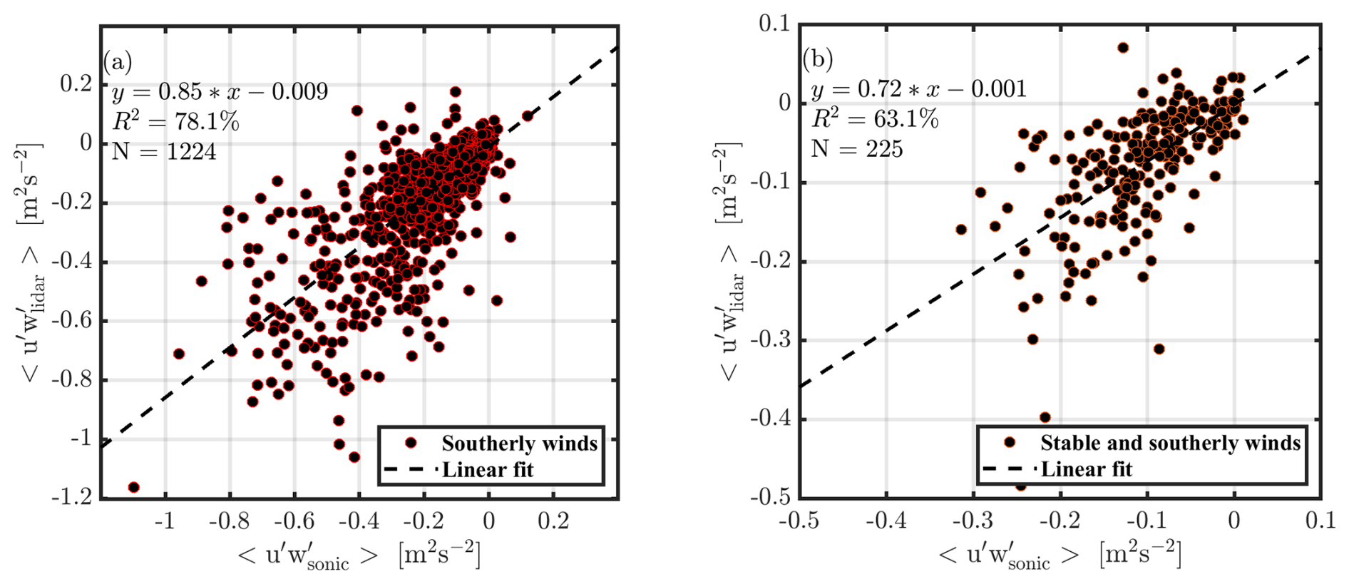
Figure A1 30 min averaged along-wind momentum flux ($\langle u^{\prime }{w}^{\prime }\rangle$) measurements from lidar at 75 m and sonic measurements at 60 m a.g.l. from 8 October 2020 to 14 January 2021 at the ARM SGP central facility for (a) southerly wind directions under all atmospheric conditions and (b) southerly wind directions under very stable atmospheric conditions (10 m <L<150 m). A linear fit between the measurements ($y=mx+c$), the coefficient of determination (R²), and the number of samples (N) are also shown. The x-axis scaling for panels (a) and (b) are different.