Flow acceleration statistics: a new paradigm for wind-driven loads, towards probabilistic turbine design

A method is developed to identify load-driving events based on filtered flow acceleration, regardless of the event-generating mechanism or specific temporal signature. Low-pass filtering enables calculation of acceleration statistics per characteristic turbine response time; this circumvents the classic problem of small-scale noise dominating observed accelerations or extremes, while providing a way to deal with different turbines and controllers. Not only is the flow acceleration physically meaningful, but its use also removes the need for de-trending. Through consideration of the 99th percentile (P₉₉) of filtered acceleration per each 10 min period, we avoid assumptions about distributions of fluctuations or turbulence and derive statistics of load-driving accelerations for offshore conditions from “fast” (10 and 20 Hz) measurements spanning more than 15 years. These statistics depend on low-pass-filter frequency (the reciprocal of turbine response time) but vary in a nontrivial manner with height due to the influence of the atmospheric boundary layer's capping inversion, as well as the surface.

We find long-term probability distributions of 10 min P₉₉ of filtered accelerations, which drive loads ranging from fatigue to ultimate; this also includes joint distributions of the P₉₉ with the 10 min mean wind speed (U) or standard deviation of horizontal wind speed fluctuations (σ_s). The long-term mean and mode of the P₉₉ of streamwise acceleration, conditioned on σ_s and U, are found to vary monotonically with σ_s and U, respectively; this corroborates the International Electrotechnical Commission (IEC) 61400-1 prescriptions for fatigue design load cases. An analogous relationship is also seen between lateral (directional) acceleration and the standard deviation of direction, particularly for submesoscale fluctuations.

The largest (extreme) P₉₉ of filtered accelerations are seen to be independent of 10 min mean speeds and have only limited connection to 10 min σ_s; traditional 10 min statistics cannot be translated into extreme load-driving acceleration statistics. From measurement heights of 100 and 160 m, time series of the 10 most extreme acceleration events per 1 m s⁻¹ wind speed bin were further investigated; events of diverse character were found to arise from numerous mechanisms, ranging from nonturbulent to turbulent flow regimes and also depending on the filter scale. Different behaviors were noted in the lateral and streamwise directions at different heights, although a small fraction of these events exhibited extreme amplitudes for both horizontal acceleration components and/or were observed at both heights within a given 10 min window. Via fits to the tails of the marginal P₉₉ distributions, curves of offshore extreme P₉₉ of filtered acceleration for return periods up to 50 years were calculated for three characteristic turbine response times (filter scales) at the observation heights of 100 and 160 m.

To drive aeroelastic simulations, Mann-model parameters were also calculated from the time series of the most extreme events, allowing constrained simulations embedding the recorded events. To facilitate this for typical industrial measurements that lack three-dimensional anemometry, a new technique for obtaining Mann-model turbulence parameters was also created; this was employed to find the parameters corresponding to the background flow behind the extremes identified and their time series. Further, a method was created to use the extreme acceleration statistics in stochastic simulations for application to loads, including interpretation within the context of the IEC 61400-1 standard. Preliminary parallel work has documented aeroelastic simulations conducted using the extreme event time series identified here, as well as Monte Carlo simulations based on the extreme statistics and new method for stochastic generation of acceleration events.

1 Introduction and background

As set out by the International Electrotechnical Commission (IEC) 61400-1 standard (IEC, 2019) for wind turbine design, fatigue load conditions are simulated in common industrial practice via the normal turbulence model (NTM), with testing of extreme loads due to transients prescribed via an extreme turbulence model (ETM) or using simplified scenarios such as the extreme operating gust (EOG), which are considered representative of critical parts of turbine design load envelopes. The magnitude of the wind events in “extreme” scenarios is prescribed by the IEC standard in terms of 10 min statistics, particularly the mean wind speed¹ U and standard deviation of wind speed σ_s or its longitudinal (streamwise) component σ_u, which are known to drive fatigue loads (Dimitrov et al., 2018). However, a growing trend towards improved turbine design has been to associate the statistics of observed phenomena (which can involve the wind as well as the turbine and electric grid) with individual design load cases (DLCs) in the 61400-1 standard and now through the emerging 61400-9 standard for probabilistic design. This has been motivated by limitations in the IEC's prescriptions for extreme cases (e.g., Dimitrov et al., 2017; Hannesdóttir et al., 2017, 2019) as well as the stochastic nature of extremes and reliability analysis (e.g., van Eijk et al., 2017; Nielsen et al., 2023).

A basis for statistical characterization efforts and constrained turbulence simulation was given by Nielsen et al. (2004), who examined gust examples and occurrence rates of wind speed jumps and identified the potential need for filtering in such characterization; however, their analysis was essentially limited to the surface-layer regime (10 m heights), where large acceleration is inextricably intertwined with ground-affected turbulence. They also identified some events with nonstationary wind and direction time series that they attributed to frontal passages and that did not appear to give large accelerations compared to the DLCs associated with wind direction changes in the IEC 61400-1 standard. However, the results were affected by the limited amount of data and were eventually superseded by later work such as that of Hannesdóttir et al. (2019). Hansen and Larsen (2007) made early comparisons of measurements to the IEC's extreme DLC for a coherent gust with direction change (ECD), focusing on the joint occurrence of jumps in wind speed and direction; however, they were limited by the small number of observations of joint events. Larsen and Hansen (2008) offered calibration of several IEC extreme DLCs, but they assumed extreme events to be turbulence driven and connected with 10 min statistics, as in the IEC 61400-1 standard.

Hannesdóttir and Kelly (2019) directly detected wind speed ramp events at heights of contemporary turbines (z ≥ 100 m) with a broad range of rise times and magnitudes, comparing their statistics to the ECD design load case; they showed that direction changes due to such events may exceed the IEC prescription. Hannesdóttir et al. (2019) found that these events did not exceed the IEC's extreme turbulence prescription, except for some events crossing rated speed (for a particular turbine and controller), which gave tower–base fore–aft loads exceeding DLC1.3 of the 61400-1. The ramp amplitudes crossing rated speed appeared to be driving the excessive loads in their aeroelastic simulations of single turbines. That extreme loads from wind ramps crossing rated speed are driven by acceleration was specifically confirmed by Kelly et al. (2021); after first obtaining long-term marginal and joint distributions of ramp (bulk) acceleration, pre-ramp speed, and upper-rotor shear for offshore wind ramp events, they used the joint probability density functions (PDFs) to generate a representative ensemble of coupled large-eddy and aeroelastic simulations² for an offshore wind farm. The simulations showed that most of the observed wind ramps, whose inferred thicknesses spanned ∼ 500 m to 10 km, persisted throughout the wind farm; they further showed that the largest thrust-based loads occur during maximal accelerations crossing rated speed.

With the above as motivation – most simply the finding that load-driving forces on turbine blades can arise from flow accelerations (F=ma) – we investigate offshore flow accelerations and the practically applicable statistics derived from them, along with connections to typical 10 min means and standard deviations; this is done for both streamwise and lateral (directional) fluctuations. We note that although a couple of studies aimed at statistics of gust-like events have recently appeared in the literature, they did not focus on offshore load-inducing flow characterization at turbine rotor heights. Shu et al. (2021) found statistical distributions for different wind gust characteristics including rise times and amplitudes, but they did not consider the associated acceleration (or the need for or effect of low-pass filtering), and their observations were from an onshore site with hills upwind. Cook (2023) also considered the big picture of gust events, reviewing and comparing numerous techniques for identifying and classifying them, with the aim of establishing an automated method; the author found that the inclusion of additional variables (temperature, pressure) improved gust classification for extreme value analysis and gave insight into the removal of anomalous spikes and use of sonic anemometry. However, Cook's (2023) study considered only surface-layer wind speeds onshore, examining maximum wind speeds rather than accelerations. The civil engineering literature has addressed gusts in the design of offshore structures for decades (Forristall, 1987; ESDU, 2012), but again this has only been in the surface layer, assuming that gusts follow turbulence statistics, and has not considered flow acceleration (despite estimates of structural acceleration). But our focus is on load-driving accelerations in the flow regimes at typical wind turbine hub heights offshore (100 m and above); such flows differ substantially compared to near-surface flow, which is dominated by turbulence associated with the surface, even more so over rough ground and terrain onshore. Further, in contrast to wind speed statistics, acceleration literally represents the forcing of the flow on turbine structures; as described later below, it does not require detrending, and with low-pass filtering, its statistics are computable for different wind turbine systems and responses.

The structure of the remaining parts of the paper is as follows: Sect. 2 outlines the data and their use, gives the methodology's basis, and demonstrates the methodology with associated statistical metrics. Section 3 presents results, showing the long-term statistics of the flow accelerations that dominate each 10 min period, considering both the frequent values that induce fatigue loads and extremes that can be associated with ultimate turbine loads. Extreme flow accelerations are examined further in Sect. 3.3–3.4, including deviation from behavior prescribed in the IEC standard and the different (often nonturbulent) flow regimes associated with such; forms are given for extrapolation of measured statistics to 50-year periods, with the goal of siting and probabilistic turbine design. For practical use, two appendices connected with Sect. 3.4 are offered. Appendix A gives a method to obtain Mann-model turbulence parameters for the flow behind extreme acceleration events, facilitating constrained simulation of such gust-like events, as well as allowing one to obtain turbulence parameters from typical industrial measurements for general use; Appendix B gives a recipe for synthesis of time series with extreme offshore flow accelerations based on the extreme acceleration distributions, including a method for probabilistic operating gusts that accounts for distributions of gust duration and its connection with acceleration amplitude. Section 4 discusses and interprets the findings, with conclusions and implications as well as ongoing/future work.

2 Data and methodology

As discussed in the introduction above, flow acceleration has been found to drive thrust-based loads during ramp-like events in operating conditions. Since wind speed ramps at turbine heights have rise times mostly ranging from roughly 10 to ∼ 300 s (Kelly et al., 2021) and gust durations in particular have been observed to be shorter (below 100 s and most commonly 10–20 s, as in Shu et al. (2021)³), we expect that 10 min statistics might not be adequate to capture extreme flow accelerations. Fast data (typically output by anemometers at a frequency of ∼ 1 Hz or higher) are known to be needed to capture gusts, as has long been documented in the civil/wind engineering literature (e.g., Davis and Newstein, 1968), meteorology (e.g., Beljaars, 1987), and recently for wind speed ramps by Hannesdóttir and Kelly (2019). In light of this and because mechanisms other than wind ramps (including phenomena other than turbulence) can cause peak loads on operating turbines, we choose a statistical methodology instead of attempting to detect or identify events with specific signatures or corresponding to particular physical mechanisms. That is, we build a statistical characterization of wind acceleration at heights impacting offshore wind turbines, with an eye towards universal description. This is done using more than 15 years (October 2004–March 2020) of high-frequency observations from the Høvsøre turbine test station, located on the west coast of Denmark (Peña et al., 2016). We select data in the offshore flow regime, defining them over the range of wind directions from 240 to 300° (which are also the most common for this wind climate) and heights that are unaffected by the coastline, which basically runs in the north–south direction. One mast was primarily employed, which provided 10 Hz speed (cup anemometer) and direction (wind vane) data from heights of 100 and 160 m; the mast's lower sensors (at 60 and 10 m) were not used due to their measurements being affected by the coastline and land below. A secondary mast 400 m to the south (the same distance to the coastline, with measurements up to 116.5 m) was also used in a supplementary manner, exploiting its three-dimensional sonic anemometers at 80 and 100 m to test three-component turbulence calculations; these “sonics” had sample rates of 20 Hz.

As a starting basis for our investigation, we consider load-driving events without joint occurrence of irregular turbine conditions, i.e., away from cut-in and cut-out. Previous studies found that the loads induced by ramp accelerations tended to be largest around rated speed, which tends to be ∼ 11–13 m s⁻¹ for multi-megawatt turbines. Further, due to the sample rates of 10–20 Hz and the need to calculate many quantities including multiple Fourier transforms for each 10 min period, we limited the number of samples processed due to computational constraints. Accordingly, to highlight flows where the rated speed is crossed and due to the immense amount of data, we select 10 min periods using the criterion $(\mathrm{8}\mathrm{m}{\mathrm{s}}^{-\mathrm{1}}+{\mathit{\sigma }}_s)\le U\le (\mathrm{18}\mathrm{m}{\mathrm{s}}^{-\mathrm{1}}-{\mathit{\sigma }}_s)$, where σ_s is the standard deviation of horizontal wind speed; the criteria σ_s>0.3 m s⁻¹ and σ_φ>0 rad s⁻¹ were also used to eliminate rare frozen anemometer and wind vane issues, where σ_φ is the standard deviation of wind direction.

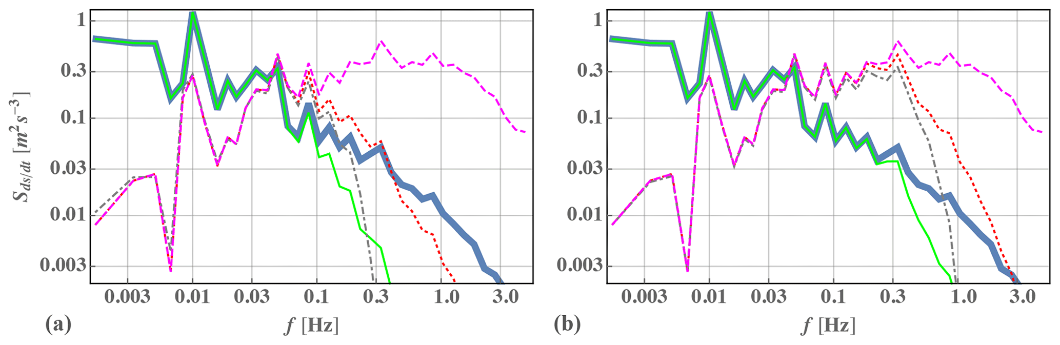
Figure 1 Spectrum of horizontal flow acceleration from one 10 min time series of a cup anemometer with a 10 Hz sample rate, calculated via different methods. Thick blue is the $\mathrm{d}s/\mathrm{d}t$ spectrum f²S_ss(f), solid green is the low-pass-filtered $\mathrm{d}s/\mathrm{d}t$ using a second-order Butterworth, dashed magenta is $\mathrm{\Delta }s/\mathrm{\Delta }t$ via a first-order finite difference, dotted-red is the Butterworth O(2) low-pass-filtered version of this $\mathrm{\Delta }s/\mathrm{\Delta }t$, and dash-dot gray is the digital differentiator with the Blackman–Nuttall window. Spectral smoothing of 12 points per decade is done to cleanly display the effects. (a) The low-pass filter has $f_{\mathrm{c}}=\mathrm{1}/\mathrm{10}$ Hz; (b) the low-pass filter has $f_{\mathrm{c}}=\mathrm{1}/\mathrm{3}$ Hz.

Nielsen et al. (2004) and others have noted that to examine the statistics of wind speed jumps, one needs to filter the wind time series. However, here we note additional details that are needed to facilitate analysis of load-driving accelerations. First, one must take care when calculating acceleration from time series: simple finite differences do not suffice due to their oscillatory spectral signature, impacting acceleration statistics in a nontrivial manner (especially the largest in each 10 min period, which is our main interest). Calculating acceleration directly in Fourier space without approximation avoids this issue:

$$\begin{array}{}\text{(1)}& \dot{s}\equiv \mathrm{d}s/\mathrm{d}t={\mathcal{F}}^{-\mathrm{1}}\left[-\mathrm{2}\mathit{\pi }if\mathcal{F}\left[s\right(t\left)\right]\right],\end{array}$$

where ℱ⁻¹ denotes the inverse Fourier transform, $S_{ss}\left(f\right)\equiv (\mathrm{2}\mathit{\pi }/T)\left|\mathcal{F}\right[s\left(t\right)]{|}^{\mathrm{2}}$ is the power spectrum of horizontal speed fluctuations s for a time series of duration T, and f denotes temporal frequency.⁴ An example of acceleration spectra from a 10 min record, including large acceleration that crosses the rated speed, is given in Fig. 1. The figure displays spectra using different methods to calculate $\dot{s}$ measured by a cup anemometer, starting with the exact calculation in Fourier space (thick blue line). Using a first-order finite-difference $\mathrm{\Delta }s/\mathrm{\Delta }t$ (dashed magenta line) to approximate $\dot{s}$, one can see significant noise at frequencies above ∼ 0.03 Hz; such noise can lead to spurious peaks in time series of the resultant approximate $\dot{s}$, impacting the largest acceleration calculated. Higher-order finite differences can somewhat improve upon the first-order approximation but still have issues; to be simple and exact, we choose direct spectral calculation of acceleration time series in this study using Eq. (1).

In addition to calculating acceleration values via a spectrally based derivative, these need to be appropriately filtered to accommodate the characteristic response of wind turbines to avoid the small-scale noise that does not impact multi-megawatt HAWTs (horizontal-axis wind turbines) due to their size. Figure 1 also displays spectra of low-pass-filtered acceleration calculated directly (green) and via finite difference (dotted red), where a second-order Butterworth filter was used. The left plot shows the filtered acceleration spectra calculated with a filter frequency $f_{\mathrm{c}}=\mathrm{1}/\mathrm{10}$ Hz, while the right-hand graph shows them using $f_{\mathrm{c}}=\mathrm{1}/\mathrm{3}$ Hz.⁵ One can see that low-pass-filtered spectra of the finite-differenced approximation $\mathrm{\Delta }s/\mathrm{\Delta }t$ also possess significant inflation of fluctuations at moderately small scales ($f>\sim \mathrm{0.05}$ Hz) compared to the unfiltered $\dot{s}$ spectrum, as well as some suppression of larger-scale fluctuations. Alternately we show the low-pass-filtered acceleration spectrum calculated via digital differentiator filter (dash-dotted gray lines) using the same f_c; like the finite-difference approximation, it displays spurious addition of noise at moderately high frequencies, albeit with a sharper spectral roll-off.⁶ From the figure it is also evident that strong artificial high-frequency fluctuations are introduced by the finite-difference approximations at high frequencies (particularly for the higher-filter frequency $f_{\mathrm{c}}=\mathrm{1}/\mathrm{3}$ Hz) and that the corresponding low-pass-filtered spectral amplitudes can exceed even the unfiltered exact acceleration spectrum; these lead to large false acceleration values, which is another reason that we both recommend and use direct spectral calculation of acceleration from here on. To allow for different turbine response times, we calculate statistics for three different low-pass-filter scales f_c, i.e., effective response times $f_{\mathrm{c}}^{-\mathrm{1}}$ = {30 s, 10 s, 3 s} using a second-order Butterworth filter.⁷

Besides direct spectral calculation of filtered acceleration, to build meaningful statistics of load-driving events, we consider the top 1 % of acceleration values per each 10 min period. In other words, we calculate P₉₉ of the filtered $\dot{s}$ for every 10 min record; from the collections of such ${\dot{s}}_{\mathrm{99}}$, we can calculate long-term statistics, according to different characteristic timescales $f_{\mathrm{c}}^{-\mathrm{1}}$. Using ${\dot{s}}_{\mathrm{99}}$ is preferable to 10 min maxima of acceleration because the latter are less certain (more likely to be outliers). For example, with a sampling rate of 10 Hz (not unusual for cup anemometers), ${\dot{s}}_{\mathrm{99}}$ corresponds to the 60th-largest value; there is considerably less statistical scatter in values that occur (at least) 60 times per 10 min period compared to a maximum that occurs just once per period. Alternately, one can consider ${\dot{s}}_{\mathrm{90}}$, i.e., the top 10 % of acceleration values for each 10 min period. For robustness, in this work we use ${\dot{s}}_{\mathrm{99}}$ as a metric for the flow accelerations expected to drive loads.

It is worth noting that we start by considering statistics of horizontal speed (such as ${\dot{s}}_{\mathrm{99}}$) because the standard instrument used in industrial wind measurement campaigns – the cup anemometer – measures fluctuations and variances in s, not the streamwise velocity component u. To be more blunt, although the IEC 61400-1 standard prescribes the use of the standard deviation of velocity components, which are dominated by the streamwise one (σ_u), in industrial practice what is presumed to be σ_u is not typically measured as such. On the contrary, from the IEC 61400-50-1 (IEC, 2022c), 61400-12-2 (IEC, 2022b), and 61400-12-1 (IEC, 2022a) standards, measurement of σ_s is prescribed when using cup anemometers, as this is what they measure (Kristensen, 2000; Yahaya and Frangi, 2004). To actually obtain σ_u requires the use of high-frequency wind vane measurements to find the corresponding high-frequency time series u(t), which permits calculation of 10 min σ_u; however, the physical separation between anemometer and wind vane can cause a directionally dependent lag between wind direction and speed, which causes a problem when measuring short-duration events. Addressing this issue is beyond the scope of the current work, and fortunately it has negligible impact on extreme events, as we see in Sect. 3 below.

2.1 Preliminary demonstration of statistical methodology

To illustrate the methodology and statistical metric described above, Fig. 2 shows how the maximum, 99th percentile, and 90th percentile of low-pass-filtered streamwise acceleration vary with the reciprocal of filter frequency (characteristic response time), using both second-order and sixth-order Butterworth filters. This is presented for two different 10 min periods of wind speeds measured at 160 m height: a “typical” period corresponding to the most commonly observed ${\dot{s}}_{\mathrm{99}}$ and ${\dot{s}}_{\mathrm{90}}$ (peak of the long-term distributions of ${\dot{s}}_{\mathrm{99}}$ or ${\dot{s}}_{\mathrm{90}}$), as well as a plot for a 10 min period corresponding to the one of the strongest streamwise flow acceleration events⁸ within the 16-year dataset. We see from Fig. 2 that the filter order has a relatively small effect on ${\dot{s}}_{\mathrm{90}}$ and ${\dot{s}}_{\mathrm{99}}$ compared to its effect on the 10 min maximum of filtered accelerations, particularly for filter timescales of 10 s or shorter; this is further justification for avoiding $max\mathit{\{}\mathrm{d}s/\mathrm{d}t\mathit{\}}$ as a metric. It also suggests that getting representative flow-driving acceleration statistics will be easier using filter scales f_c of $\mathrm{1}/\mathrm{10}$ or $\mathrm{1}/\mathrm{3}$ Hz in contrast to choosing $\mathrm{1}/\mathrm{30}$ Hz; the latter corresponds to a characteristic response time of 30 s, which is longer than that corresponding to most commercial wind turbines. It is perhaps unsurprising that lower f_c (longer characteristic response times) result in smaller acceleration magnitudes, as smaller f_c mean more of the signal is filtered away, particularly the shortest Δt jumps that can have larger values of $\mathrm{\Delta }s/\mathrm{\Delta }t$ (as shown also in Kelly et al., 2021,​​​​​​​ and Appendix B).

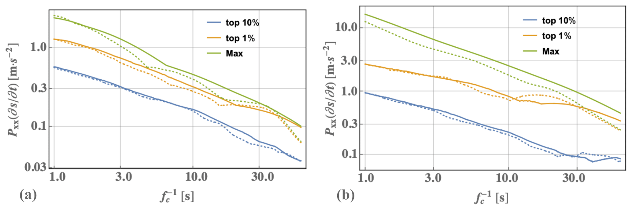
Figure 2 Dependences of the 90th percentile, 99th percentile, and maximum of low-pass-filtered acceleration versus the reciprocal of filter frequency (characteristic response time) for wind speeds recorded at 160 m height over two different 10 min periods. Solid and dotted lines indicate second- and sixth-order low-pass-filtered acceleration, respectively, using a low-pass Butterworth filter. Panel (a) is the typical/common record; panel (b) is the case with extreme acceleration (the highest in the 12–13 m s⁻¹ wind speed bin for the dataset).

We note that while Nielsen et al. (2004) identified a need for a “third-order filter to avoid cascading”, where the latter refers to an increasing number of jumps counted with shorter durations, they were concerned with counting occurrences of wind speed crossing above a threshold (progressively zooming in to the threshold: at smaller and smaller scales, more crossings are found). Here we are not counting crossing events but rather calculating exceedance statistics of filtered accelerations for each 10 min period; using ${\dot{s}}_{\mathrm{99}}$ (or ${\dot{s}}_{\mathrm{90}}$) avoids the need for a higher-order filter, and as shown above and in Fig. 2, the filter order does not significantly impact this statistic.

3 Analysis and results

With an aim towards probabilistic turbine design, using the filtered flow acceleration statistics and measurements introduced above, we will derive a climatology of (long-term) offshore load-driving accelerations and associated exceedance rates. This includes long-term statistics of filtered $\mathrm{d}s/\mathrm{d}t$, as well as filtered directional acceleration via the derivative of wind direction, $\mathrm{d}\mathit{\phi }/\mathrm{d}t$.

3.1 Horizontal and streamwise flow accelerations

Because cup anemometers are the standard instrument used for wind energy in tandem with wind vanes (much more often than two- or three-dimensional sonic anemometers), we continue with temporal derivatives of horizontal wind speed, $\dot{s}$; later we will also consider the streamwise and lateral components of acceleration (i.e., filtered $\mathrm{d}u/\mathrm{d}t$ and $\mathrm{d}v/\mathrm{d}t)$.

The long-term probability density of 10 min 99th-percentile low-pass-filtered horizontal acceleration, $P\left({\dot{s}}_{\mathrm{99}}\right)$, is plotted in Fig. 3 for the two primary heights considered (100 and 160 m above the sea) and for three different low-pass-filter scales f_c ($\mathrm{1}/\mathrm{3}$, $\mathrm{1}/\mathrm{10}$, and $\mathrm{1}/\mathrm{30}$ Hz). This gives context for the previous figure, showing that the right-hand plot of Fig. 2 corresponds to a 10 min period containing an extreme acceleration event, while the left-hand plot in Fig. 2 matches a period where the filtered acceleration is near the most commonly occurring 10 min filtered ${\dot{s}}_{\mathrm{99}}$; from the two plots in Fig. 2 and for a filter frequency of 0.1 Hz, the ${\dot{s}}_{\mathrm{99}}$ at 160 m are approximately 0.3 and 0.7 m s⁻², respectively.

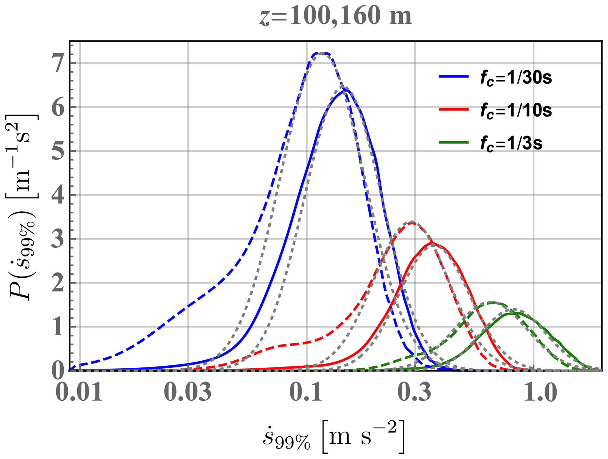
Figure 3 Long-term distribution of flow accelerations: the PDF of 10 min P₉₉'s​​​​​​​ of filtered $\mathrm{d}s/\mathrm{d}t$, for three different filter scales from measurements at 100 m (solid) and 160 m height (dashed). Dotted gray lines are log-normal fits.

The range of wind speeds considered (8–18 m s⁻¹) occurs 61 % of the time for fully offshore flow at the Høvsøre site, so the actual number of ${\dot{s}}_{\mathrm{99}}$ values detected for a given acceleration bin (increment) over the years analyzed would be larger than what was detected. Here we assume that the probability density $P\left({\dot{s}}_{\mathrm{99}}\right)$ shown in Fig. 3 would not change if we could include wind speeds below 8 m s⁻¹ and above 18 m s⁻¹, i.e., no significant bias arising from differences between $P\left({\dot{s}}_{\mathrm{99}}|U<\mathrm{8}\mathrm{m}{\mathrm{s}}^{-\mathrm{1}}\right)$ and $P\left({\dot{s}}_{\mathrm{99}}|U>\mathrm{18}\mathrm{m}{\mathrm{s}}^{-\mathrm{1}}\right)$. One can further note from Fig. 3 that larger ${\dot{s}}_{\mathrm{99}}$ are seen at 100 m compared to 160 m, including the most extreme accelerations. However, because atmospheric boundary layer (ABL) depths shallower than 200 m are uncommon offshore (Liu and Liang, 2010; Ratnam and Basha, 2010), it is possible that for heights above 160 m, the ${\dot{s}}_{\mathrm{99}}$ could be still larger than at 100 m due to effects from the ABL capping inversion.

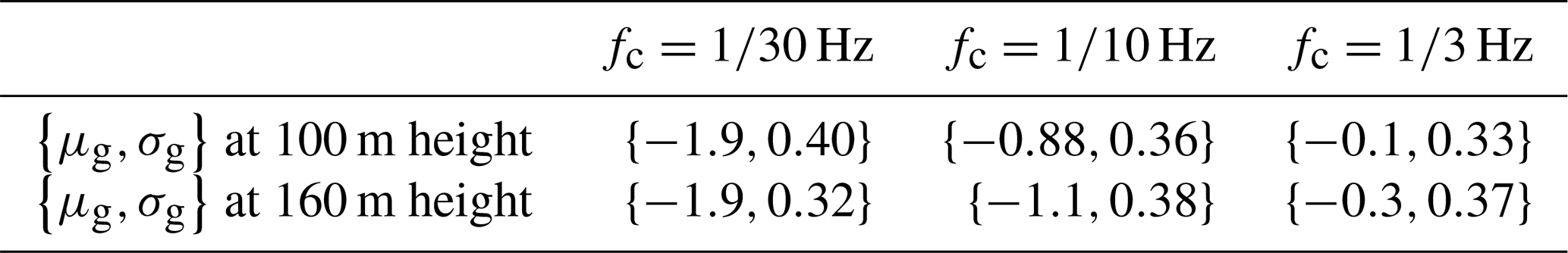
Table 1 Log-normal parameters fitted around peaks (most common values) of the ${\dot{s}}_{\mathrm{99}}$ distributions.​​​​​​​

The PDF of ${\dot{s}}_{\mathrm{99}}$ follows a log-normal form around its peak, so the most commonly occurring (fatigue) load-driving acceleration values can be approximated with the oft-used log-normal distribution:

$$\begin{array}{}\text{(2)}& P\left({\dot{s}}_{\mathrm{99}}\right)={\left({\dot{s}}_{\mathrm{99}}{\mathit{\sigma }}_{\mathrm{g}}\sqrt{\mathrm{2}\mathit{\pi }}\right)}^{-\mathrm{1}}\exp \left[{\displaystyle \frac{-\mathrm{1}}{\mathrm{2}}}{\left({\displaystyle \frac{\ln \left({\dot{s}}_{\mathrm{99}}\right)-{\mathit{\mu }}_{\mathrm{g}}}{{\mathit{\sigma }}_{\mathrm{g}}}}\right)}^{\mathrm{2}}\right].\end{array}$$

Here the dimensionless geometric (multiplicative) standard deviation parameter is defined using $e^{{\mathit{\sigma }}_{\mathrm{g}}^{\mathrm{2}}}\equiv \mathrm{1}+{\left({\mathit{\sigma }}_{{\dot{s}}_{\mathrm{99}}}/{\mathit{\mu }}_{{\dot{s}}_{\mathrm{99}}}\right)}^{\mathrm{2}}$, and the analogous geometric-mean⁹ parameter is $e^{{\mathit{\mu }}_{\mathrm{g}}}\equiv {\mathit{\mu }}_{{\dot{s}}_{\mathrm{99}}}{e}^{-{\mathit{\sigma }}_{\mathrm{g}}^{\mathrm{2}}/\mathrm{2}}={\mathit{\mu }}_{{\dot{s}}_{\mathrm{99}}}{\left[\mathrm{1}+{\left({\mathit{\sigma }}_{{\dot{s}}_{\mathrm{99}}}/{\mathit{\mu }}_{{\dot{s}}_{\mathrm{99}}}\right)}^{\mathrm{2}}\right]}^{-\mathrm{1}/\mathrm{2}}$; the latter is equivalent to the commonly seen definition ${\mathit{\mu }}_{\mathrm{g}}\equiv \ln \left[{\mathit{\mu }}_{{\dot{s}}_{\mathrm{99}}}^{\mathrm{2}}/{\left({\mathit{\mu }}_{{\dot{s}}_{\mathrm{99}}}^{\mathrm{2}}+{\mathit{\sigma }}_{{\dot{s}}_{\mathrm{99}}}^{\mathrm{2}}\right)}^{\mathrm{1}/\mathrm{2}}\right]$. Fits around the peak give log-normal parameter values {μ_g,σ_g} for each filter scale considered at z = 100 and 160 m, which are shown in Table 1. The peaks seen in Fig. 3 correspond to the mode of ${\dot{s}}_{\mathrm{99}}$. We note that although analytically $\mathrm{Mo}\mathit{\left\{}{\dot{s}}_{\mathrm{99}}\mathit{\right\}}=e^{{\mathit{\mu }}_{\mathrm{g}}-{\mathit{\sigma }}_{\mathrm{g}}^{\mathrm{2}}}={\mathit{\mu }}_{{\dot{s}}_{\mathrm{99}}}{\left[\mathrm{1}+{\left({\mathit{\sigma }}_{{\dot{s}}_{\mathrm{99}}}/{\mathit{\mu }}_{{\dot{s}}_{\mathrm{99}}}\right)}^{\mathrm{2}}\right]}^{-\mathrm{3}/\mathrm{2}}$ for the log-normal form, this is not used, and the mode is found numerically (via histogram) because the tails of $P\left({\dot{s}}_{\mathrm{99}}\right)$ do not follow the same distribution.

Table 2 Fitted log-normal distribution parameters for extrapolation of the highest (extreme) acceleration.

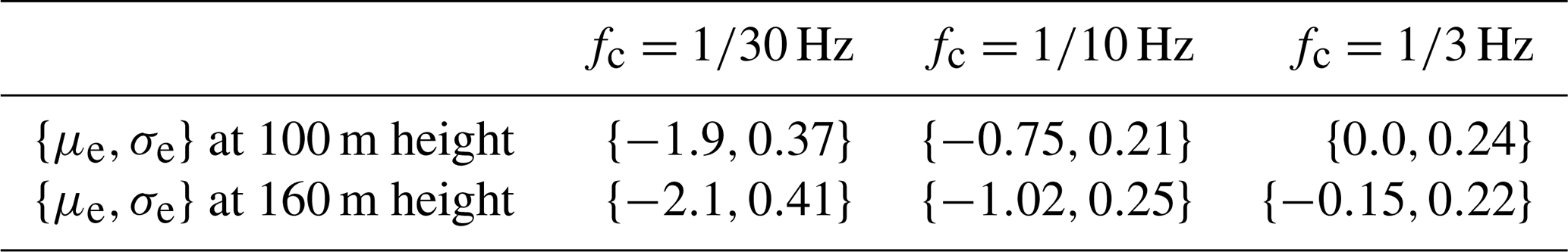
The largest observed ${\dot{s}}_{\mathrm{99}}$ do not conform to the overall log-normal fits, as the latter capture the most likely ${\dot{s}}_{\mathrm{99}}$ around the peak of its distributions. However, the extreme tails of $P\left({\dot{s}}_{\mathrm{99}}\right)$ are also seen to follow a different log-normal distribution, simply with different log-normal parameter values (for the heights and filter scales considered). The extreme ${\dot{s}}_{\mathrm{99}}$ are shown in Fig. 4, which displays the exceedance probability (i.e., survival function,¹⁰ SF) of ${\dot{s}}_{\mathrm{99}}$ for the two heights and three filter scales considered. Fitting the log-normal distribution to the largest ${\dot{s}}_{\mathrm{99}}$ for all three filter scales at 100 and 160 m heights, we obtain the log-normal parameters {μ_e,σ_e} for extreme flow accelerations; their values are shown in Table 2, and the distributions corresponding to these log-normal fits are shown by the dotted gray lines in Fig. 4.

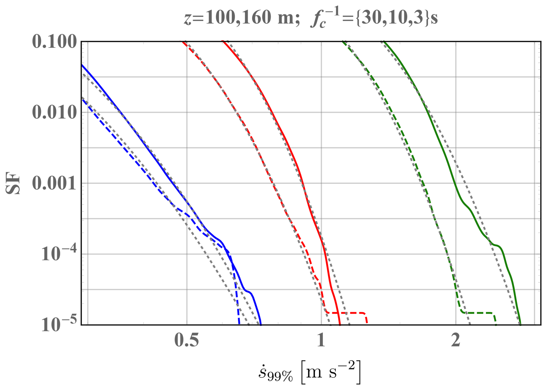
Figure 4 Survival function ($\mathrm{SF}=\mathrm{1}-\mathrm{CDF}$) of the 10 min P₉₉ of streamwise filtered accelerations (i.e., ${\dot{s}}_{\mathrm{99}\mathit{\%}}$) for the two heights (solid lines are 100 m; dashed lines are 160 m) and three filter scales ($f_{\mathrm{c}}^{-\mathrm{1}}$ = 30 s in blue, $f_{\mathrm{c}}^{-\mathrm{1}}$ = 10 s in red, $f_{\mathrm{c}}^{-\mathrm{1}}$ = 3 s in green) considered; dotted gray lines are the extreme fits using a log-normal distribution.

From the figure one sees that for the top 1–10 values of ${\dot{s}}_{\mathrm{99}}$, the plots can become irregular due to the rarity of such events (< once per year), deviating somewhat from the log-normal fits; this is also expected, noting that $\mathrm{SF}={\mathrm{10}}^{-\mathrm{5}}$ corresponds to one occurrence in roughly 2 years, whereas for the range of directions and speeds considered from the 16-year dataset, we have 67 648​​​​​​​ 10 min periods or a minimum SF of approximately $\mathrm{1.5}\times {\mathrm{10}}^{-\mathrm{5}}$. We note that unlike what one might expect from inertial-range turbulence, the curves of extreme $P\left({\dot{s}}_{\mathrm{99}}\right)$ at both heights cannot be collapsed through a simple relation in terms of filter scale f_c; scaling the 1 % most extreme $P\left({\dot{s}}_{\mathrm{99}}\right)$ by a factor $f_{\mathrm{c}}^{\mathrm{0.62}}$ causes coincidence of only the f_c = $\mathrm{1}/\mathrm{3}$ and $\mathrm{1}/\mathrm{30}$ Hz curves at 100 m height and the f_c = $\mathrm{1}/\mathrm{3}$ and $\mathrm{1}/\mathrm{10}$ Hz curves at 160 m height (not shown). We expect this because different mechanisms with different timescales are responsible for extreme flow acceleration events at different heights due to the relative distance to the capping inversion; this is examined later in Sect. 3.3.2.

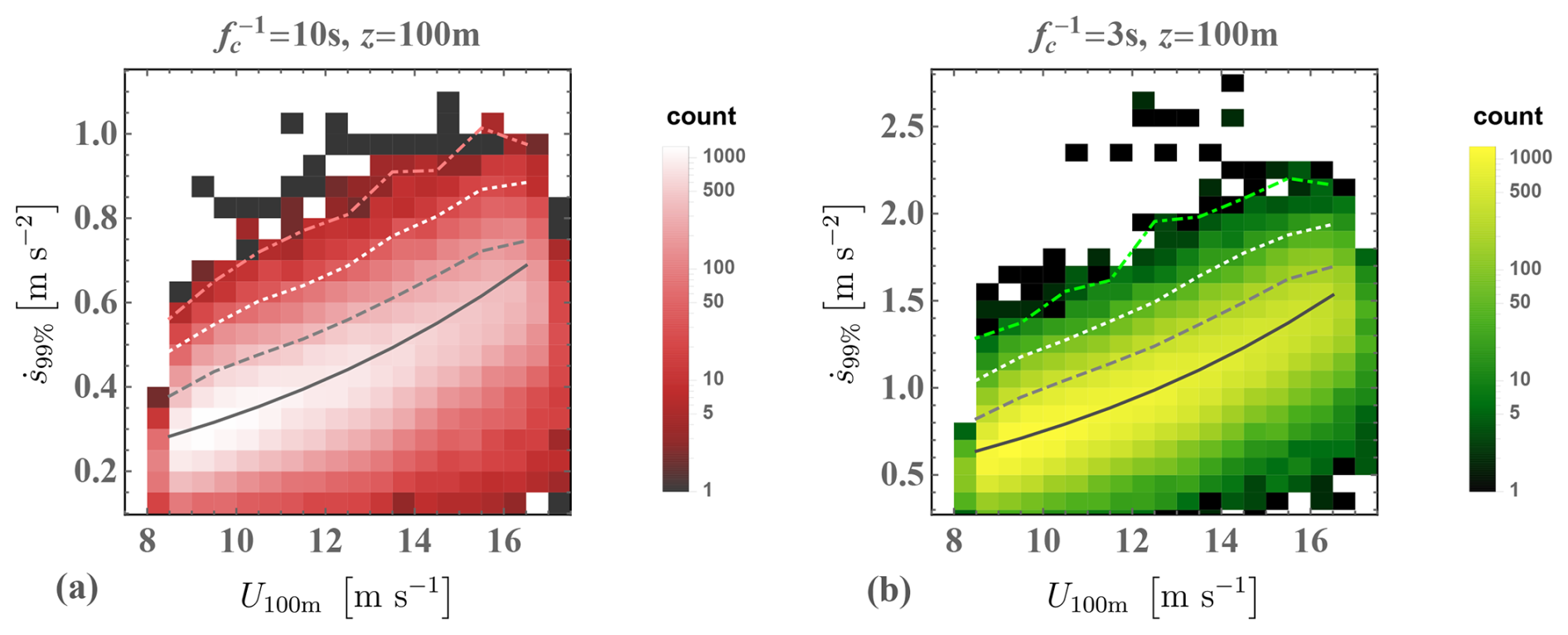
Figure 5 Joint distribution of 10 min P₉₉ of filtered $\mathrm{d}s/\mathrm{d}t$ and mean wind speed at 100 m height for low-pass-filter scales of 0.1 Hz (a) and $\mathrm{1}/\mathrm{3}$ Hz (b). The solid line is an exponential fit to the mode of ${\dot{s}}_{\mathrm{99}}$ conditioned on U, dashed gray is the 90th percentile, dotted white is the 99th percentile, and dash-dotted color is the 99.9th percentile of $P\left({\dot{s}}_{\mathrm{99}}|U\right)$.

The joint distribution of 10 min ${\dot{s}}_{\mathrm{99}}$ and mean wind speed, i.e., $P\left({\dot{s}}_{\mathrm{99}}U\right)$, gives more information about the character of streamwise load-driving accelerations; this is shown in Fig. 5 for the measurements from 100 m height for filter scales of 0.1 and $\mathrm{1}/\mathrm{3}$ Hz. We note that essentially the same plots result for 160 m height (not shown), although with slightly smaller accelerations. The figure indicates that stronger ${\dot{s}}_{\mathrm{99}}$ generally occur for higher wind speeds. The most commonly occurring 10 min filtered ${\dot{s}}_{\mathrm{99}}$ exhibit an exponential dependence on wind speed: the mode conditional on speed is described by $\mathrm{Mo}\left\{{\dot{s}}_{\mathrm{99}}|U\right\}\approx a_{\mathrm{md}}{e}^{-\left(U/U_{\mathrm{md}}\right)}$, where U_md≃9 m s⁻¹ and $a_{\mathrm{md}}\simeq \mathrm{0.3}\cdot \mathrm{Mo}\left\{{\dot{s}}_{\mathrm{99}}\right\}$, which for the cases at z = 100 m in Fig. 5 are $a_{\mathrm{md}}{|}_{f_{\mathrm{c}}=\mathrm{0.1}\mathrm{Hz}}\approx \mathrm{0.11}$ m s⁻² and $a_{\mathrm{md}}{|}_{f_{\mathrm{c}}=\mathrm{1}/\mathrm{3}\mathrm{Hz}}\approx \mathrm{0.25}$ m s⁻². The 90th and 99th percentile of ${\dot{s}}_{\mathrm{99}}$ conditioned on U are seen to grow approximately linearly with U, while the 99.9th percentile of $P\left({\dot{s}}_{\mathrm{99}}|U\right)$ grows more slowly with speed. Nevertheless, no clear speed dependence for the most extreme ${\dot{s}}_{\mathrm{99}}$ has been found (at either height), as seen in Fig. 5. One might assume this to be a sampling artifact and presume that extreme ${\dot{s}}_{\mathrm{99}}$ grows with U like the 99.9th percentile of $P\left({\dot{s}}_{\mathrm{99}}|U\right)$; however, as will be seen below in Sect. 3.3, the time series for the most extreme ${\dot{s}}_{\mathrm{99}}$ show that the largest flow accelerations can be separate from the background flow or turbulence. Furthermore, the slower growth of the top 0.1 % of $P\left({\dot{s}}_{\mathrm{99}}|U\right)$ with U compared to the top 1 % of $P\left({\dot{s}}_{\mathrm{99}}|U\right)$ implies that more extreme accelerations will have a weaker dependence on wind speed, and we also see in the figure that a larger number of extreme events occur between 14 and 16 m s⁻¹ compared to 12–14 m s⁻¹; thus it appears most likely that extreme ${\dot{s}}_{\mathrm{99}}$ are essentially independent of wind speed at these heights for the range of speeds analyzed.

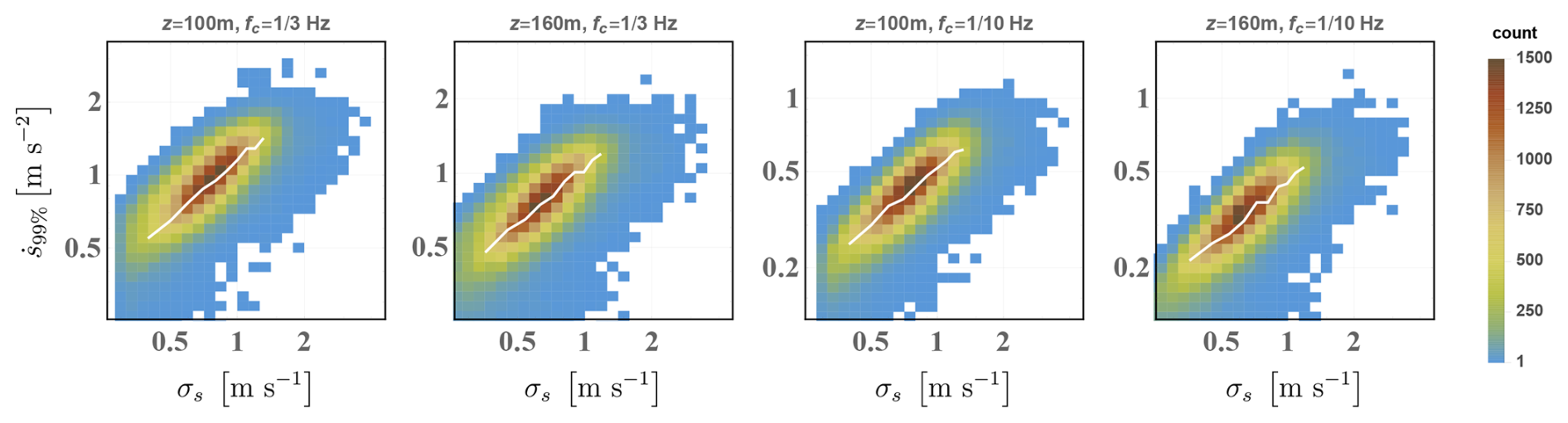
Figure 6 Joint PDFs $P\left({\dot{s}}_{\mathrm{99}},{\mathit{\sigma }}_s\right)$ of all 10 min P₉₉ of filtered acceleration and the standard deviation of wind speed at both heights analyzed for low-pass-filter scales f_c = 0.1 Hz and f_c = $\mathrm{1}/\mathrm{3}$ Hz. White lines show the mode of ${\dot{s}}_{\mathrm{99}}$ conditioned on σ_s.

The long-term behavior of ${\dot{s}}_{\mathrm{99}}$, considering its potential relation to turbine loads, can be further examined in terms of the commonly used 10 min standard deviation of wind speed σ_s (or alternately, streamwise velocity σ_u). Figure 6 shows the joint distribution $P\left({\dot{s}}_{\mathrm{99}},{\mathit{\sigma }}_s\right)$ for low-pass-filter scales f_c of 0.1 and $\mathrm{1}/\mathrm{3}$ Hz at both 100 and 160 m heights. The correlation of all $\left\{{\dot{s}}_{\mathrm{99}},{\mathit{\sigma }}_s\right\}$ are found to range from 0.73 for $f_{\mathrm{c}}=\mathrm{1}/\mathrm{3}$ Hz to 0.83 for $f_{\mathrm{c}}=\mathrm{1}/\mathrm{30}$ Hz, with commonly occurring ${\dot{s}}_{\mathrm{99}}$ and σ_s exhibiting still higher correlation; the plots exhibit a simple monotonic dependence of ${\dot{s}}_{\mathrm{99}}$ on σ_s around the conditional mode of ${\dot{s}}_{\mathrm{99}}|{\mathit{\sigma }}_s$. For values of σ_s between 0.4 and 1.3 m s (where the joint CDF is between roughly 5 % and 95 %, i.e., rejecting less common joint values), the mode follows a power law, $\mathrm{Mo}\left\{{\dot{s}}_{\mathrm{99}}|{\mathit{\sigma }}_s\right\}\approx c_{\mathit{\sigma }}{\mathit{\sigma }}_s^{\mathit{\beta }}$, where β ranges from 0.75 to 0.8 for the range of f_c and heights analyzed; the constant is c_σ≈1.1 for $f_{\mathrm{c}}=\mathrm{1}/\mathrm{3}$ Hz and c_σ≈0.4 for $f_{\mathrm{c}}=\mathrm{1}/\mathrm{10}$ Hz. One could try to derive a similar relation based on idealized theoretical arguments, but we avoid that here; this is because we do not know the horizontal turbulence length scale for every 10 min period, and additionally, we would also need to account for the non-Gaussianity that occurs around extreme acceleration events (shown later below). The simple monotonic dependence of frequently occurring ${\dot{s}}_{\mathrm{99}}$ on σ_s and their high correlation are expected since for typical turbulent offshore flow (over a homogeneous surface), larger variability in acceleration reflected by ${\dot{s}}_{\mathrm{99}}$ is connected with larger variability in speed. This result, along with the analogous behavior with wind speed seen in Fig. 5, is also consistent with the IEC 61400-1 standard's prescriptions for fatigue loads based on σ_s and σ_s∝U. However, Fig. 6 also shows that more extreme acceleration events do not appear to exhibit a dependence on σ_s; although the largest ${\dot{s}}_{\mathrm{99}}$ tend to occur for σ_s above ∼ 0.5 m s⁻¹, the maximum observed ${\dot{s}}_{\mathrm{99}}$ are flat over the range of observed σ_s from 0.5 to 4 m s⁻¹.

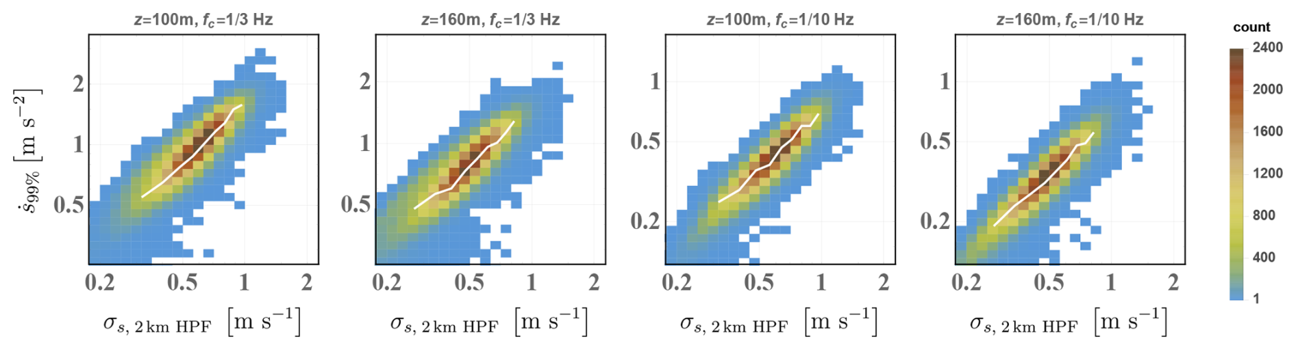
Figure 7 Joint PDFs $P\left({\dot{s}}_{\mathrm{99}},{\mathit{\sigma }}_{s,\mathrm{3}\mathrm{km}\mathrm{HPF}}\right)$ of all 10 min P₉₉ of filtered acceleration and the standard deviation of spatially high-pass-filtered wind speed σ_{s, 3 km HPF}, where scales larger than 2 km are filtered out of σ_s. As in Fig. 6, results are given at both heights analyzed for the acceleration low-pass-filter scales f_c = 0.1 Hz and f_c = $\mathrm{1}/\mathrm{3}$ Hz. White lines show the mode of ${\dot{s}}_{\mathrm{99}}$ conditioned on σ_{s, 3 km HPF}.

As noted by Larsen and Hansen (2014), for fatigue loads it is important to separate microscale wind speed variability from larger-scale (mesoscale) fluctuations; this is conventionally done by removing the latter through 10 min trend removal¹¹, which is simply a form of high-pass filtering. Thus we now examine the relationship between ${\dot{s}}_{\mathrm{99}}$ and high-pass-filtered σ_s; using a second-order high-pass Butterworth filter, we remove mesoscale fluctuations in the frequency domain with a high-pass length scale $l_{\mathrm{cH}}=\mathrm{2}\mathit{\pi }/k_{\mathrm{cH}}=\mathrm{2}$ km via Taylor's hypothesis ($f_{\mathrm{cH}}=U/l_{\mathrm{cH}}$), as in Hannesdóttir and Kelly (2019), to get a “microscale” variance σ_s,HP for every 10 min time series analyzed. Analogous to the $P\left({\dot{s}}_{\mathrm{99}},{\mathit{\sigma }}_s\right)$ shown in Fig. 6, the joint distribution of ${\dot{s}}_{\mathrm{99}}$ and σ_s,HP is displayed in Fig. 7. From the figure, we see that ${\dot{s}}_{\mathrm{99}}$ follows σ_s,HP more closely than it tracks σ_s. This is expected, since acceleration can be seen spectrally as a sort of high-pass-filtered wind speed following Eq. (1) (i.e., multiplication of the power spectral density of speed by f² removes trends and low-frequency fluctuations). Accordingly, the correlation between ${\dot{s}}_{\mathrm{99}}$ and σ_s,HP is found to be 0.9 ± 0.02, higher than between ${\dot{s}}_{\mathrm{99}}$ and σ_s; counterintuitively, the spatial high-pass filtering also causes the ${\dot{s}}_{\mathrm{99}}$ and σ_s,HP correlation to become essentially independent of f_c. Furthermore, the conditional mode $\mathrm{Mo}\left\{{\dot{s}}_{\mathrm{99}}|{\mathit{\sigma }}_{s,\mathrm{HP}}\right\}$ grows almost linearly with σ_s,HP (a power law with exponent β ranging from 0.9 to 1.03), with the linear approximation $\mathrm{Mo}\left\{{\dot{s}}_{\mathrm{99}}|{\mathit{\sigma }}_{s,\mathrm{HP}}\right\}\approx c_{\mathit{\sigma }\mathrm{HP}}{\mathit{\sigma }}_{s,\mathrm{HP}}$ having a proportionality constant of order 1¹². This is again consistent with the IEC 61400-1 prescription to use the de-trended wind speed standard deviation. In contrast, from Fig. 7 we see that extreme ${\dot{s}}_{\mathrm{99}}$ do not exhibit a clear dependence on σ_s,HP, similar to Fig. 6 for $P\left({\dot{s}}_{\mathrm{99}},{\mathit{\sigma }}_s\right)$. However, the same level of extreme acceleration occurs over a narrower range of σ_s,HP compared to σ_s. The lack of clear dependence on σ_s,HP (as well as σ_s) may be due in part to limited sampling, whereby a larger dataset (yet longer measurement period) might indicate (some) increase in extreme ${\dot{s}}_{\mathrm{99}}$ with σ_s,HP for σ_s,HP1 m s⁻¹.

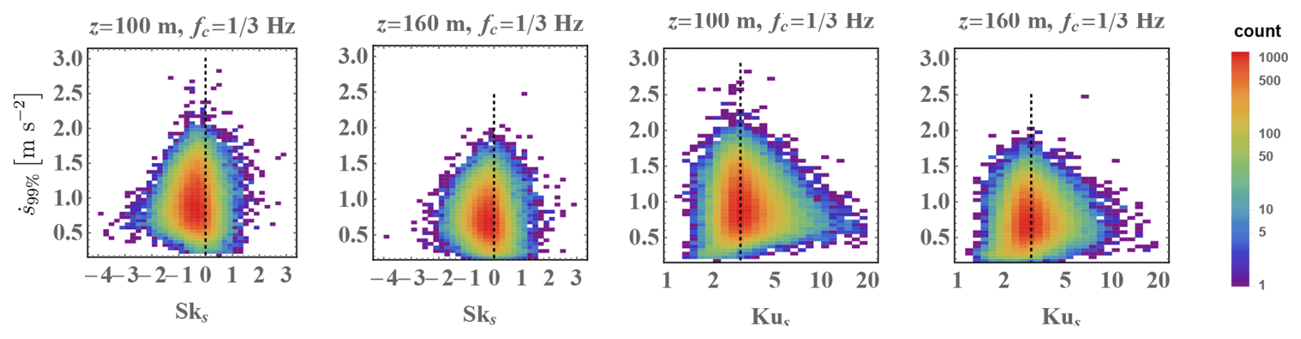
Figure 8 Joint PDF of P₉₉ of low-pass-filtered accelerations with either skewness or kurtosis of wind speed; results are shown for both 100 and 160 m heights. A logarithmic scale is used for joint PDF colors. Dotted lines denote Gaussian values (Sk_s = 0 and Ku_s = 3).

Previous work has presumed that extreme load-driving flow phenomena tend to be associated with non-Gaussian turbulence (e.g., Moriarty et al., 2004; Nielsen et al., 2004) and due to nonstationary conditions (Chen et al., 2007). However, as demonstrated in Fig. 8, the observations appear to indicate the opposite, in terms of the skewness of horizontal speed (Sk_s): the most frequently occurring values of Sk_s show modestly non-Gaussian behavior, with Sk_s<0. The figure displays the joint distribution of ${\dot{s}}_{\mathrm{99}}$ for $f_{\mathrm{c}}=\mathrm{1}/\mathrm{3}$ Hz with skewness and kurtosis at both 100 and 160 m heights. Overall, ${\dot{s}}_{\mathrm{99}}$ does not show a correlation with Sk_s, and extreme ${\dot{s}}_{\mathrm{99}}$ are coincident with vanishing or slightly negative Sk_s, appearing to follow from the same distribution of Sk_s as more commonly occurring values. Figure 8 also shows the joint distribution of ${\dot{s}}_{\mathrm{99}}$ and kurtosis of wind speed (Ku_s), which indicates that ${\dot{s}}_{\mathrm{99}}$ shows no correlation with Ku_s and that both the most common and extreme values of the 10 min P₉₉ of flow acceleration correspond to the Gaussian kurtosis value Ku_s=3. We further note that the same qualitative results occur for ${\dot{s}}_{\mathrm{99}}$ calculated using lower f_c (not shown). The lack of correlation between extreme ${\dot{s}}_{\mathrm{99}}$ and either Sk_s or Ku_s, as well as the limited dependence of large ${\dot{s}}_{\mathrm{99}}$ on σ_s, suggests that a given extreme ${\dot{s}}_{\mathrm{99}}$ is not necessarily connected with the underlying distribution of wind speed fluctuations or turbulence in the associated 10 min period. Rather, an event is caused by one or more flow phenomena that include a large acceleration with a duration much smaller than 10 min, which is effectively superposed on the background flow and its fluctuations. This is confirmed directly in Sect. 3.3 below by examining observed time series corresponding to the largest recorded ${\dot{s}}_{\mathrm{99}}$; there we will also see that many extreme events are not associated with nonstationary conditions (i.e., there is not necessarily a jump from some lower speed to a higher one). Further, it follows that (at least some) extreme load-driving accelerations cannot be predicted using 10 min statistics.

Vertical differences

Statistics of the difference in acceleration between 100 and 160 m were also calculated using the three f_c considered, including the 99th percentile of horizontal (and streamwise) acceleration. The most common P₉₉ of $\mathrm{\Delta }\dot{s}$ (including the mode) were found to be proportional to and ∼ 15 %–30 % higher than ${\dot{s}}_{\mathrm{99}}$ averaged over the two heights, with more variability found for lower f_c. This is shown in Fig. 9. The figure also shows that extreme values of $P_{\mathrm{99}}\left(\mathrm{\Delta }\dot{s}\right)$ can be twice as large as the ${\dot{s}}_{\mathrm{99}}$ averaged over the two heights. However, such statistics do not account for when the respective acceleration occurred at the two heights within each 10 min period. To do so requires further analysis due to the time lag associated with the physical shape of acceleration-inducing flow structures (e.g., ramp-like events detected by Hannesdóttir et al., 2017, or inclination angles of cold fronts); identifying the signatures of individual events within a 10 min period and matching these at multiple heights (e.g., Suomi et al., 2015) or locations is beyond the scope of this work. Still, the differences over a Δz of 60 m may lead to large flap-wise blade root bending moments for both fatigue and ultimate loads. As with the ${\dot{s}}_{\mathrm{99}}$ investigated earlier, for $P_{\mathrm{99}}\left(\mathrm{\Delta }\dot{s}\right)$ across two heights, the high-pass spatially filtered standard deviation of wind speed is a reasonable surrogate for commonly occurring $P_{\mathrm{99}}\left(\mathrm{\Delta }\dot{s}\right)$ due to the linear relationship exhibited between $P_{\mathrm{99}}\left(\mathrm{\Delta }\dot{s}\right)$ and ${\dot{s}}_{\mathrm{99}}$ around the conditional mode, $\mathrm{Mo}\left\{P_{\mathrm{99}}\left(\mathrm{\Delta }\dot{s}\right)|{\dot{s}}_{\mathrm{99}}\right\}$; this is also consistent with the IEC 61400-1 standard's use of detrended σ_s for design load cases that drive flap-wise bending moments.

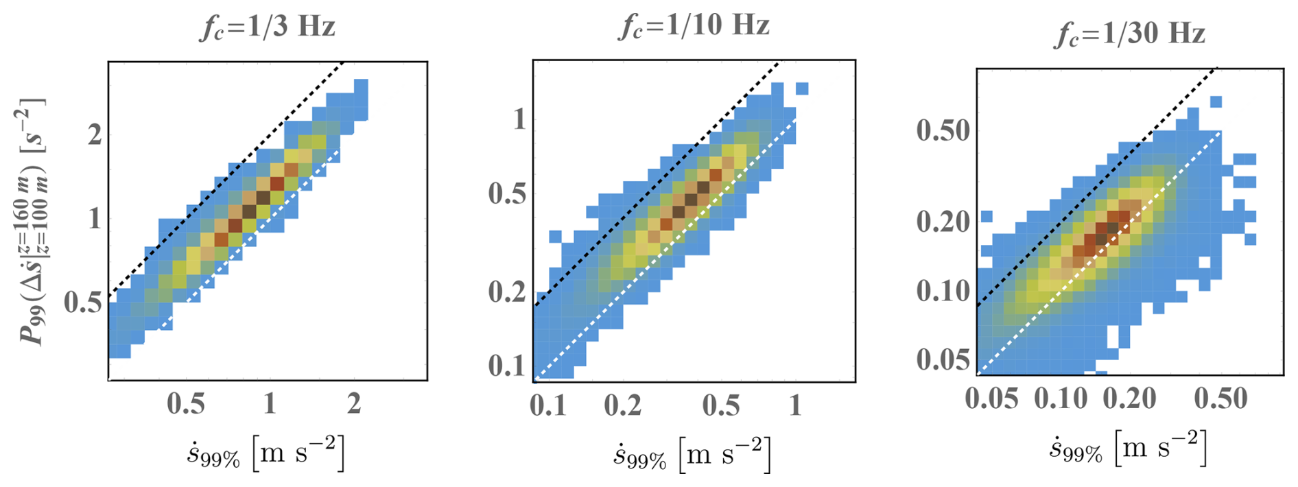
Figure 9 P₉₉ of the difference in low-pass-filtered acceleration between 100 and 160 m versus the P₉₉ of low-pass-filtered acceleration averaged over the two heights (plotted joint PDF) for all three low-pass-filter scales considered. The dotted white line shows the 1 : 1 relationship; dotted black is 2 : 1.

Regarding shear, we also report that there is no pattern or correlation between $\mathrm{\Delta }U/\mathrm{\Delta }z$ and P₉₉ of $\mathrm{\Delta }\dot{s}$ or $\dot{s}$. This again points toward acceleration that is associated with events separate from the underlying flow or turbulence (when the flow is turbulent), with the acceleration-causing events in effect superposed upon the background.

3.2 Directional and transverse flow acceleration

Following the streamwise acceleration considered in the previous sections, here we consider lateral acceleration, expressible through the time rate of change in direction $\dot{\mathit{\phi }}\equiv \mathrm{d}\mathit{\phi }/\mathrm{d}t$. In Cartesian coordinates (denoted by subscript c) defined by the mean wind direction at a given height, the direction is defined by ${\mathit{\phi }}_{\mathrm{c}}\equiv \arctan \left(v_{\mathrm{c}}/u_{\mathrm{c}}\right)$, which gives $\dot{v}={\dot{\mathit{\phi }}}_{\mathrm{c}}u\left[\mathrm{1}+{\left(v/u\right)}^{\mathrm{2}}\right]+\dot{u}v/u=\left({\dot{\mathit{\phi }}}_{\mathrm{c}}{s}^{\mathrm{2}}+\dot{u}v\right)/u$; using units of radians per second for $\dot{\mathit{\phi }}$ then gives $\dot{v}$ in the conventional unit of acceleration (m s⁻²). In the coordinate system used in wind energy (based on the incoming wind direction, increasing clockwise) one then has $\dot{\mathit{\phi }}=-{\dot{\mathit{\phi }}}_{\mathrm{c}}$ so that $\dot{v}=\left(-\dot{\mathit{\phi }}{s}^{\mathrm{2}}+\dot{u}v\right)/u$. Since the horizontal acceleration $\mathrm{d}\left(\sqrt{u^{\mathrm{2}}+v^{\mathrm{2}}}\right)/\mathrm{d}t$ can be written as

$$\begin{array}{}\text{(3)}& \dot{s}=\left(\dot{u}u+\dot{v}v\right)/s,\end{array}$$

one can then express the lateral component of acceleration as

$$\begin{array}{}\text{(4)}& \dot{v}=\left(-\dot{\mathit{\phi }}u+\dot{s}v/s\right)=\left(-\dot{\mathit{\phi }}s\cos \mathit{\phi }+\dot{s}\sin \mathit{\phi }\right)\end{array}$$

and the streamwise component as

$$\begin{array}{}\text{(5)}& \dot{u}=\left(\dot{s}u/s-\dot{\mathit{\phi }}v\right)=\left(\dot{s}\cos \mathit{\phi }-\dot{\mathit{\phi }}s\sin \mathit{\phi }\right).\end{array}$$

Typically, $v/u\ll \mathrm{1}$ so that $\dot{v}\simeq -\dot{\mathit{\phi }}u\approx -\dot{\mathit{\phi }}s$, although for strong lateral fluctuations or low wind speeds, this approximation might be expected to become inaccurate. However, for the range of wind speeds considered here (8–18 m s⁻¹) and noting that we will be using statistics of the strongest 1 % of acceleration values from each 10 min period (denoted ${\dot{\mathit{\phi }}}_{\mathrm{99}}$), this approximation becomes reasonable.¹³ The strongest 1 % of $\dot{\mathit{\phi }}$ can be either positive or negative since it is found that the top 1 % of leftward and rightward acceleration in a given 10 min period is on average the same (symmetric); i.e., flipping the sign of $\dot{\mathit{\phi }}$, we find that its CDF above 0.99 (or SF below 0.01, i.e., the top 1 %) is unchanged.

As with $\dot{s}$ analyzed above, the quantity $\dot{\mathit{\phi }}$ is calculated in the Fourier domain to avoid spurious values that can arise due to finite differencing. We again apply a spatial second-order Butterworth high-pass filter via Taylor's hypothesis with filter frequency $f_{\mathrm{c}}=U/\mathrm{2}$ km to decompose the standard deviation σ_φ into the mesoscale and microscale components, where the Yamartino (1984) method is employed to calculate standard deviations of direction.

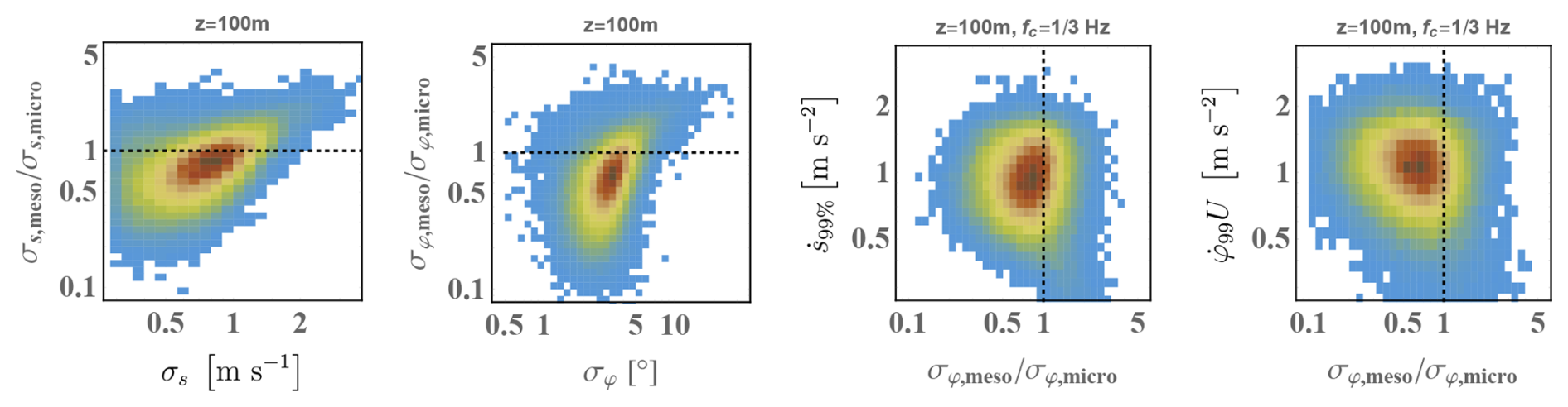
Figure 10 Joint behavior (as joint PDFs), with the ratio of mesoscale (> 2 km) to microscale (< 2 km) directional variability. Left – the ratio of the respective mesoscale to microscale standard deviations versus σ_s and σ_φ; right – P₉₉ of acceleration and the corresponding ratio ${\mathit{\sigma }}_{\mathrm{meso}}/{\mathit{\sigma }}_{\mathrm{micro}}$. The dotted line indicates ${\mathit{\sigma }}_{s,\mathrm{meso}}/{\mathit{\sigma }}_{s,\mathrm{micro}}=\mathrm{1}$ and ${\mathit{\sigma }}_{\mathit{\phi },\mathrm{meso}}/{\mathit{\sigma }}_{\mathit{\phi },\mathrm{micro}}=\mathrm{1}$.

Like σ_s, the 10 min standard deviation of direction σ_φ is dictated most often by fluctuations having spatial extents smaller than 2 km (microscale), with a minority of cases where larger-scale fluctuations dominate. On the other hand, strong variability in speed or direction at rotor heights (here 100–160 m) tends to be more associated with mesoscale structures – and not with microscale turbulence. This is shown by the left-hand plots in Fig. 10, which indicate that for σ_φ≳10°, the mesoscale portion of σ_φ (larger than 2 km) exceeds the microscale part of σ_φ, and similarly for σ_s≳2 m s⁻¹, the mesoscale part of σ_s exceeds the microscale part. However, this is not the case for the dominant acceleration, as demonstrated by the right-hand plots of Fig. 10, which visualize the statistics of 10 min P₉₉ of temporally low-pass-filtered $\dot{s}$ (i.e., ${\dot{s}}_{\mathrm{99}}$, third plot) and directional acceleration (approximated¹⁴ via $\dot{\mathit{\phi }}U$ in the rightmost plot). The plots show that there is little correlation between these P₉₉ and ${\mathit{\sigma }}_{\mathit{\phi },\mathrm{meso}}/{\mathit{\sigma }}_{\mathit{\phi },\mathrm{micro}}$, with the extreme acceleration particularly independent of ${\mathit{\sigma }}_{\mathit{\phi },\mathrm{meso}}/{\mathit{\sigma }}_{\mathit{\phi },\mathrm{micro}}$. This is consistent with extreme flow accelerations having temporal scales longer than ∼ 3 s but shorter than ∼ 2 min (via Taylor's hypothesis: 2 km divided by the highest speeds analyzed, 18 m s⁻¹). The results shown in Fig. 10 are for $f_{\mathrm{c}}=\mathrm{1}/\mathrm{3}$ Hz at 100 m height, but the same results occur at 160 m height and for the other f_c (0.1 and $\mathrm{1}/\mathrm{30}$ Hz) for which ${\dot{\mathit{\phi }}}_{\mathrm{99}}$ and ${\dot{s}}_{\mathrm{99}}$ were calculated.

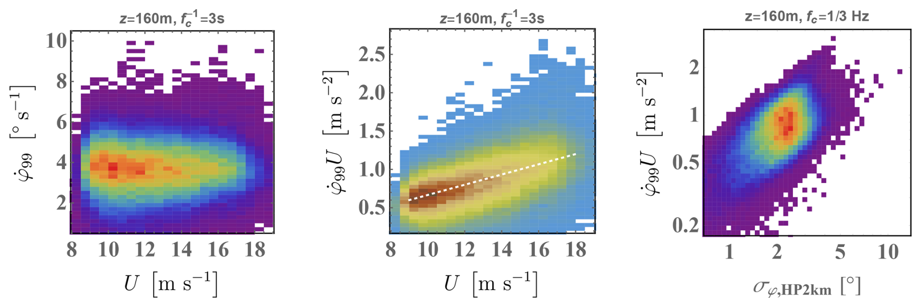
Figure 11 Joint distributions of the rate of change in wind direction and lateral acceleration with mean wind speed and microscale variability in direction (scales less than ∼ 2 km). The dotted white line in $P\left({\dot{\mathit{\phi }}}_{\mathrm{99}}U,U\right)$ shows the linear relationship around the conditional mode $\mathrm{Mo}\mathit{\left\{}{\dot{\mathit{\phi }}}_{\mathrm{99}}U\right|U\mathit{\}}$.

In contrast to ${\dot{s}}_{\mathrm{99}}$ or streamwise acceleration, ${\dot{\mathit{\phi }}}_{\mathrm{99}}$ does not exhibit a wind speed dependence; however, the directional acceleration and ${\dot{\mathit{\phi }}}_{\mathrm{99}}U\approx {\dot{v}}_{\mathrm{99}}$ do have a dependence on U, analogous to that of ${\dot{s}}_{\mathrm{99}}$ (and presumably ${\dot{u}}_{\mathrm{99}}$). This is shown in the two left-hand plots of Fig. 11 for z=160 m and f_c=0.1 Hz, with the same behavior also observed at 100 m height for all f_c (not shown). In essence, the mode and commonly observed values of ${\dot{\mathit{\phi }}}_{\mathrm{99}}U$ (and thus ${\dot{v}}_{\mathrm{99}}$) increase linearly with mean wind speed U, while extreme values of ${\dot{\mathit{\phi }}}_{\mathrm{99}}U$ lack any dependence on wind speed. The right-hand plot of Fig. 11 also shows that, analogous to the joint behavior of ${\dot{s}}_{\mathrm{99}}$ with σ_s and σ_s,micro, the envelope of possible lateral accelerations represented by ${\dot{\mathit{\phi }}}_{\mathrm{99}}U$ increases proportionally with the microscale part of the standard deviation of direction, σ_φ,micro (less precisely with σ_φ, not depicted), with extreme ${\dot{\mathit{\phi }}}_{\mathrm{99}}U$ having a limited dependence on σ_φ,micro (or σ_φ), although possibly increasing with σ_φ,micro but limited by sampling, similar to how $P\left({\dot{s}}_{\mathrm{99}},{\mathit{\sigma }}_{s,\mathrm{micro}}\right)$ was. In contrast to $\mathrm{Mo}\left\{{\dot{s}}_{\mathrm{99}}|{\mathit{\sigma }}_s\right\}$ and its relationship with σ_s, the most common directional accelerations and conditional mode $\mathrm{Mo}\left\{{\dot{\mathit{\phi }}}_{\mathrm{99}}U|{\mathit{\sigma }}_{\mathit{\phi }}\right\}$ appear to be independent of σ_φ.

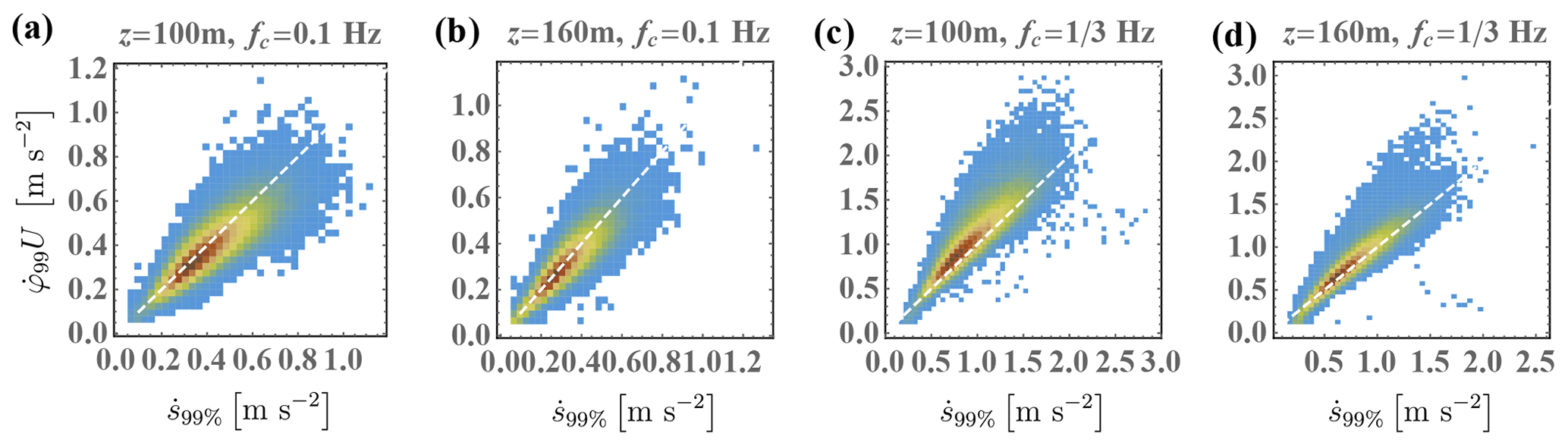
Figure 12 Joint PDF of the 99th percentile of the directional and horizontal flow acceleration calculated as $\dot{\mathit{\phi }}U$ and $\dot{s}$, respectively, plotted at both 100 and 160 m heights for characteristic response times ($f_{\mathrm{c}}^{-\mathrm{1}}$) of 10 s (a, b) and 3 s (c, d). Note that linear axes are used here; log–log plots give joint PDF shapes similar to those shown in Figs. 6, 7, and 9. The dashed white line indicates a 1 : 1 relation.

The joint behavior of lateral and streamwise flow acceleration is shown in Fig. 12, which gives $P\left({\dot{s}}_{\mathrm{99}},{\dot{\mathit{\phi }}}_{\mathrm{99}}U\right)$ at both 100 and 160 m heights for f_c = $\mathrm{1}/\mathrm{10}$ and $\mathrm{1}/\mathrm{3}$ Hz. From the figure we see that for f_c = $\mathrm{1}/\mathrm{10}$ Hz, the most commonly occurring conditions have P₉₉ of streamwise and lateral acceleration that are approximately equal, whereas for the higher filter frequency of f_c = $\mathrm{1}/\mathrm{3}$ Hz, we see that the lateral P₉₉ of acceleration exceed the streamwise for common conditions. This is likely because inertial-range turbulence is not filtered out for f_c = $\mathrm{1}/\mathrm{3}$ Hz (with crosswind fluctuations being $\mathrm{4}/\mathrm{3}$ larger than the lateral ones at the smallest scales). Using more severe low-pass filtering, with $f_{\mathrm{c}}=\mathrm{1}/\mathrm{30}$ Hz (not shown), the opposite trend occurs and the most frequently occurring conditions have larger ${\dot{s}}_{\mathrm{99}}$ than ${\dot{\mathit{\phi }}}_{\mathrm{99}}U$. Regarding the less common and extreme acceleration values, the plots in Fig. 12 are made with linear axes to illustrate how the variability in load-driving acceleration increases. However, we note that when plotted using log–log axes, the joint PDFs resemble those in Figs. 6, 7, and 9; i.e., the joint variability around the mode (width of the joint PDF envelope perpendicular to the 1 : 1 line) is relatively constant in log space, scaling geometrically and consistently with log-normal distributions. The extreme acceleration events do not exhibit a clear trend, but one can see that a fraction of extreme events involve both streamwise and lateral components. Further, comparing the extreme values between the plots of Fig. 12, one can see that for different f_c (again corresponding to different turbine/controller response times), different events comprise the extremes. Some extremes with durations shorter than 10 s appear for $f_{\mathrm{c}}=\mathrm{1}/\mathrm{3}$ Hz but are filtered out for f_c = $\mathrm{1}/\mathrm{10}$ Hz, particularly streamwise events without significant lateral accelerations. Recalling that the lateral 10 min P₉₉ of acceleration ${\dot{v}}_{\mathrm{99}}$ may be approximated by ${\dot{\mathit{\phi }}}_{\mathrm{99}}U$ and analogously the streamwise ${\dot{u}}_{\mathrm{99}}$ approximated by ${\dot{s}}_{\mathrm{99}}$, we point out that the “missing” pieces (${\dot{v}}_{\mathrm{99}}-{\dot{\mathit{\phi }}}_{\mathrm{99}}U$ and ${\dot{u}}_{\mathrm{99}}-{\dot{s}}_{\mathrm{99}}$) are not only small but also similarly behaved, so a bias is not expected in the joint variations shown in Fig. 12. In the next section we will show how this looks for a sample joint extreme event, along with the strongest flow acceleration events measured over the 15 years of observations. Since three-dimensional sonic anemometer recordings were available only at 80 m for most of the measurement period, our extensive set of calculations were made using ${\dot{\mathit{\phi }}}_{\mathrm{99}}$ and ${\dot{s}}_{\mathrm{99}}$; future work includes re-calculation to obtain filtered ${\dot{u}}_{\mathrm{99}}$ and ${\dot{v}}_{\mathrm{99}}$ via a combination of the anemometer and wind vane measurements, as these cannot be obtained through postprocessing of the data used and the results reported here.

3.3 Extreme flow accelerations

3.3.1 Anatomy of an extreme event

To gain insight into what happens during an extreme acceleration event, we examine the acceleration components and wind speed together during a period containing such an event. Figure 13 shows the 10 min segment for which the largest ${\dot{s}}_{\mathrm{99}}$ with a low-pass-filter scale of 0.1 Hz was found for 10 min mean speeds in the range of 11–12 m s⁻¹ at 100 m height, i.e., $max\left\{{\dot{s}}_{\mathrm{99}}|{\left(\mathrm{11}\le U<\mathrm{12}\mathrm{m}{\mathrm{s}}^{-\mathrm{1}}\right)}_{f_{\mathrm{c}}=\mathrm{0.1}\mathrm{Hz}}\right\}$; this was also the second-strongest ${\dot{s}}_{\mathrm{99}}$ in this U bin for $f_{\mathrm{c}}=\mathrm{1}/\mathrm{3}$ Hz, and the plots in the figure show results using $f_{\mathrm{c}}=\mathrm{1}/\mathrm{3}$ Hz. This extreme event was chosen due to not only its magnitude but also its occurrence during a limited time for which additional concurrent data were available: three-dimensional sonic anemometer data from 100 and 160 m heights on the same mast (denoted LM, which hosts the cup anemometers and wind vanes whose data we have presented thus far), as well as at z = 80 m from a second mast (MM) located 400 m to the south. The upper-left plot of Fig. 13 shows the “path” of $\left\{\dot{u},\dot{v}\right\}$, i.e., the evolution of vector acceleration, measured by a three-dimensional sonic anemometer with a sample rate f_s = 20 Hz. For comparison, the upper-middle plot of the figure shows $\dot{s}$ with the directional acceleration (as $\dot{\mathit{\phi }}U$) calculated using the same three-dimensional anemometer. Several extreme flow acceleration events are seen to occur, ranging from lateral to streamwise relative to the 10 min mean wind direction, with $\dot{u}$ and $\dot{v}$ having similar maximum amplitudes. Comparing the $\left\{\dot{u},\dot{v}\right\}$ and $\left\{\dot{s},\dot{\mathit{\phi }}U\right\}$ paths, we see that they are nearly identical, with slight distortions in the lateral estimate $\dot{\mathit{\phi }}U$ as expected and discussed following Eq. (4).¹⁵ The largest distortions only indirectly affect the 99th percentile values of filtered acceleration since ${\dot{s}}_{\mathrm{99}}$ corresponds to the 120th-largest value of $\dot{s}$ in a 10 min period for f_s = 20 Hz (and the 60th-largest value for cup anemometers with f_s = 10 Hz); while the maxima of filtered $\dot{s}$ and $\dot{u}$ exceed 3 m s⁻² for the case shown in the figure, ${\dot{s}}_{\mathrm{99}}=\mathrm{1.6}$ m s⁻² and ${\dot{u}}_{\mathrm{99}}=\mathrm{1.5}$ m s⁻² for f_c = $\mathrm{1}/\mathrm{3}$ Hz. The upper-right-hand plot of Fig. 13 displays the evolution of filtered acceleration with speed s, given as a joint PDF to additionally indicate the distribution of speeds during the 10 min; the path of $\left\{s,\dot{s}\right\}$ evolves counterclockwise ($\dot{s}>\mathrm{0}$ leads to increasing speed, $\dot{s}<\mathrm{0}$ to decreasing speed). We also see that $\dot{s}>{\dot{s}}_{\mathrm{99}}$ occurs across a range of wind speeds from ∼ 8 to 15 m s⁻¹, with the largest $\dot{s}$ involving a jump from ∼ 8 to 12 m s⁻¹. In this 10 min period with σ_s=1.5 m s⁻¹, the speed varies far beyond the 11–12 m s⁻¹ range defining the conditional mean; s < 11 m s⁻¹ for nearly half the period and s > 13 m s⁻¹ for more than 1 min, with s repeatedly crossing the typical rated speed (ca. 12 m s⁻¹ for multi-megawatt turbines). This is further illustrated in the middle plot, which displays the time series of speed and vertical velocity at 100 m and 160 m. It shows that similar speeds (and ranges of $\dot{s}$) occur at 100 and 160 m heights, although sometimes $\dot{s}{|}_{z=\mathrm{160}\mathrm{m}}$ has the opposite sign as $\dot{s}{|}_{z=\mathrm{100}\mathrm{m}}$; this is related to significant vertical motions ($\left|w\right|$ > 1 m s⁻¹) occurring at both heights, with a time lag (along with small directional changes). The middle plot also displays s(t) from a cup anemometer at 100 m height on the same boom as the sonic anemometer, separated by about 5 m in the north–south direction; from it, we see that the cup records nearly the same speed and does not exhibit the “overspeeding” that can occur due to large lateral velocity variance in some cup anemometers (Kristensen, 1998), despite the occurrence of large crosswind acceleration, including instances where $\dot{v}>\dot{u}$.

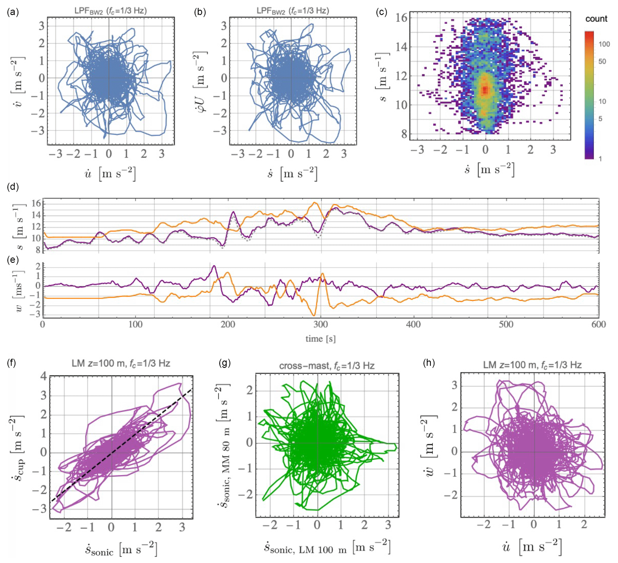
Figure 13 Anatomy of a 10 min period of extreme ${\dot{s}}_{\mathrm{99}}$ at a height of 100 m with low-pass-filter scale $f_{\mathrm{c}}=\mathrm{1}/\mathrm{3}$ Hz. (a) Path of the horizontal acceleration vector from the sonic anemometer; (b) path of $\mathit{\{}\dot{s},\dot{\mathit{\phi }}U\mathit{\}}$ from sonic; and (c) path of $\dot{s}$ and speed s, plotted as a joint PDF. (d, e) Time series of low-pass-filtered speed and the vertical velocity component (sonic at 100 m is purple, sonic at 160 m is orange, cup at 100 m is dotted gray). (f) $\dot{s}$ at 100 m height from cup and sonic anemometers; (g) $\dot{s}$ from two masts separated by ca. 400 m, with z = 80 m and z = 100 m; and (h) filtered acceleration components $\mathit{\{}\dot{u},\dot{w}\mathit{\}}$ at 100 m.

The lower-left plot of Fig. 13 shows filtered $\dot{s}$ from the cup and sonic anemometers at 100 m, and their evolution together indicates that both anemometers are essentially measuring the same magnitudes of filtered acceleration, although with slightly larger $\left|\dot{s}\right|$ from the cup for the most extreme $\dot{s}$ that occurred around t≃200–210 s. The correlation function between them gives no persistent time lag, which is consistent with the anemometer separation being perpendicular to the wind direction of ∼ 270 ± 15° recorded for this case; the flow structures passing the mast appear to have lateral dimensions greater than 5 m and pass the sensors at z = 100 m simultaneously. The lower-middle plot of Fig. 13 shows the mutual path of filtered $\dot{s}$ from the sonic anemometers at 80 m height from the mast 400 m to the south (MM) and at z = 100 m on the main mast (LM) used thus far. The acceleration values are effectively uncorrelated, although a persistent cross-correlation (ρ>0.6) between the speeds is found for lags of ∼ 50–100 s, suggesting that the flow structures have lateral extents of at least 400 m and even larger streamwise extent (via Taylor's hypothesis), possibly propagating at an angle relative to the mean wind or evolving at different rates in the crosswind direction. The existence of significant vertical acceleration is shown in the lower-right plot of Fig. 13 from the sonic anemometer at 100 m, with the extreme magnitudes of $\dot{w}$ exceeding those of $\dot{u}$; these are essentially uncorrelated statistically, but one can see from the $\left\{\dot{u},\dot{w}\right\}$ plot that during the extreme jumps in wind speed, they are sometimes related (with varying lag), also noting such from the time series.

3.3.2 Long-term extreme statistics: a collection of phenomena

The 10 most extreme acceleration magnitude events were detected in each 1 m s⁻¹ increment of 10 min mean wind speed between 8 and 17 m s⁻¹ at both 100 and 160 m heights; i.e., 180 streamwise acceleration events (10 events × 9 speed bins × 2 heights) were found, with the corresponding 10 min time series of speed and direction saved for use in constrained turbulence simulations to drive aeroelastic load calculations (McWilliam et al., 2023a).¹⁶ The time series s(t) for the most extreme ${\dot{s}}_{\mathrm{99}}$ in each U bin are shown in Fig. 14 for a low-pass-filter frequency of 0.1 Hz.

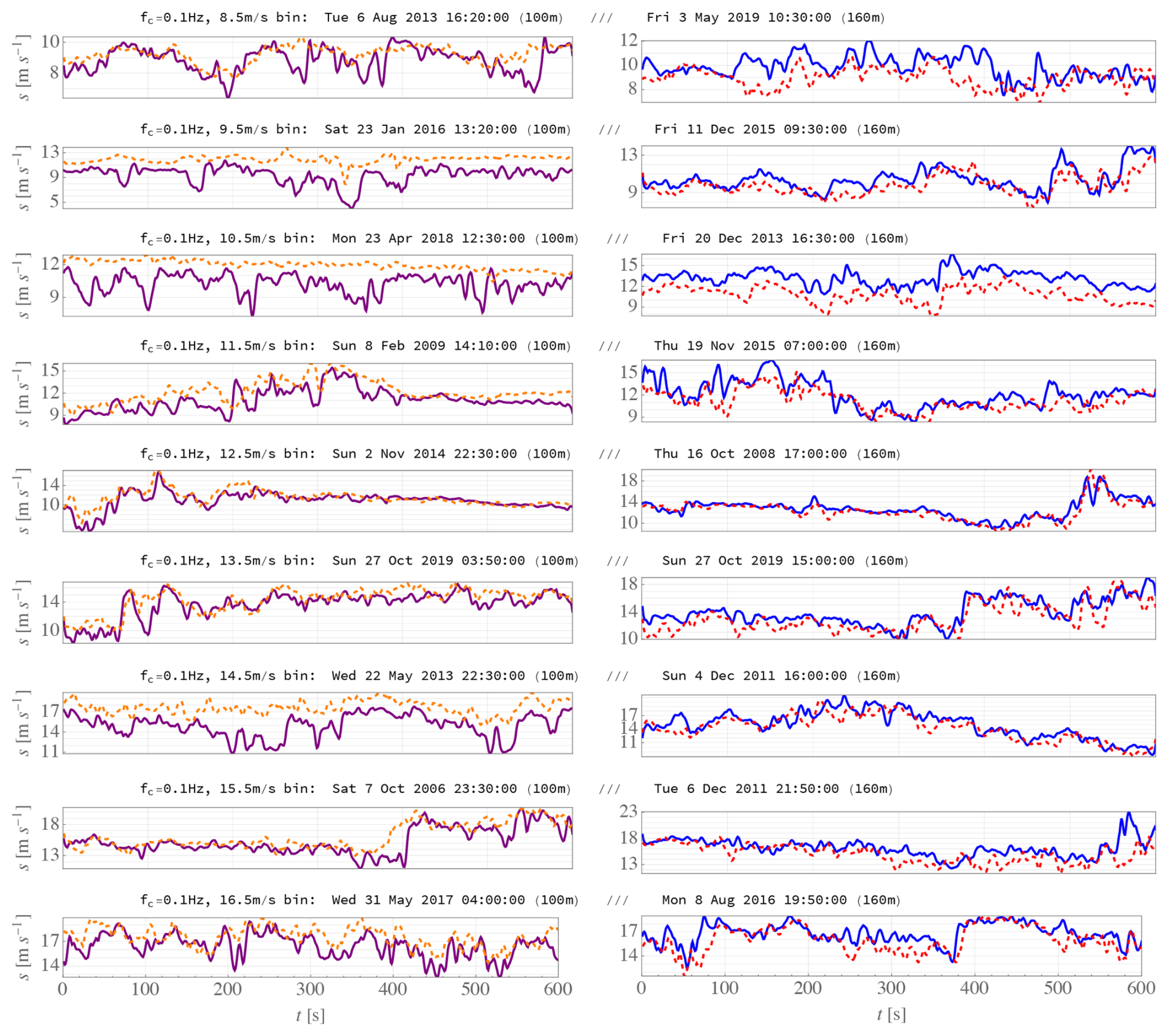
Figure 14 Pairs of 10 min time series s(t) for the most extreme acceleration events in each 1 m s⁻¹ wind speed bin for the low-pass-filter scale of 0.1 Hz. Left – 100 m events (purple s|_100 m, dashed orange s|_160 m); right – 160 m events (blue s|_160 m, dashed red s|_100 m).

The most extreme events detected at 100 m were different from those at 160 m, and the top ${\dot{s}}_{\mathrm{99}}$ periods detected with f_c = 0.1 Hz are generally different than those found when f_c = $\mathrm{1}/\mathrm{3}$ Hz (not shown). However, we note that for a given U, the most extreme event at one height and f_c is often one of the most extreme events found for another {z,f_c}, such as the case shown previously in Fig. 13. As can be inferred from the time series shown in Fig. 14, a number of different qualitative properties and corresponding meteorological phenomena are associated with these extreme events. First, for some of the 100 m events (left-side plots in Fig. 14), one can see that the corresponding 160 m speeds are constant or look like a smoother version of s(t) at 100 m, particularly for smaller mean speed bins (below typical rated speeds). These correspond to shallow ABL depths that can occur during winter or nighttime in nontropical climates (e.g., Liu and Liang, 2010; Kelly et al., 2014), where the anemometer at 160 m height is near or within the stable inversion where turbulence is suppressed. The cases where s_160 m follows s_100 m tend to correspond to being just below the inversion, associated with breaking gravity waves or wave turbulence (Finnigan et al., 1984; Einaudi and Finnigan, 1993), as is the top case for f_c = 0.1 Hz in the wind speed range $\mathrm{8}<U_{\mathrm{100}\mathrm{m}}\le \mathrm{9}$ m s⁻¹, or entrainment-zone turbulence (Otte and Wyngaard, 2001) as in the cases for $\mathrm{14}<U\le \mathrm{15}$ m s⁻¹ at both heights¹⁷ with f_c = 0.1 Hz (Fig. 14). The cases with “flat” U_160 m likely correspond to shallow ABL depths below 160 m having sufficiently strong capping inversions such that turbulence is suppressed. At higher speeds (above ∼ 11 m s⁻¹), the extreme acceleration events at 100 m also tended to be accompanied by significant acceleration at 160 m, which is consistent with the irregular spatial structure of the ABL capping inversion (Sullivan et al., 1998). Unfortunately, consistent ceilometer data from Høvsøre were not available to quantify the ABL depths during these periods with extreme ${\dot{s}}_{\mathrm{99}}$.

For the top extreme events detected at 160 m (right-hand plots of Fig. 14), the acceleration-associated jumps in wind speed were mostly accompanied by similar fluctuations at 100 m, consistent with ABL depths near 160 m. Further, for some of these events, one can also see steady winds before or after the jumps, commensurate with inversion depths fluctuating across this height. For several speeds, nonstationarity also occurred at both 100 and 160 m during daytime hours, consistent with frontal passage; this included two wind speed ramp events.

Further identification of these events and confirmation of their driving mechanisms may be accomplished through analysis of mesoscale simulations for the site, which is left for future work. Time series of the top 10 events in each mean speed bin for f_c=0.1 Hz were provided to and used by McWilliam et al. (2023b) for aeroelastic simulations, along with Mann-model turbulence parameters corresponding to each respective period found from the cup–vane combinations via a new method (see Appendix A). The time series in that dataset were provided as 1 Hz (down-sampled from 10 Hz) records of the speed, direction, streamwise velocity component, and lateral velocity component at both 100 and 160 m heights; the reader may obtain these from the reference dataset of McWilliam et al. (2023a).

3.4 Load-driving accelerations, from fatigue to ultimate

Aiming at practical use and enabling comparison with wind turbine standards, the behavior of dominant filtered accelerations has been examined via the top 1 % of every 10 min period, i.e., using ${\dot{s}}_{\mathrm{99}}$ and ${\dot{\mathit{\phi }}}_{\mathrm{99}}$; this includes statistics conditional on the mean wind speeds U and the corresponding standard deviation (σ_s or σ_φ), as described in the previous sections. The most common values of horizontal (streamwise) and directional (lateral) 99th-percentile acceleration, calculated here via ${\dot{s}}_{\mathrm{99}}$ and ${\dot{\mathit{\phi }}}_{\mathrm{99}}s$, are presumably what drive some fatigue loads on wind turbines, particularly thrust-based loads such as the flap-wise root bending moment and tower base fore–aft moment (Frandsen, 2007; Kelly et al., 2021). Although the most commonly occurring ${\dot{s}}_{\mathrm{99}}$ have been shown above to be analytically describable through the conditional modes $\mathrm{Mo}\left\{{\dot{s}}_{\mathrm{99}}|U\right\}$ and $\mathrm{Mo}\left\{{\dot{s}}_{\mathrm{99}}|{\mathit{\sigma }}_s\right\}$, current industrial practices and the IEC 61400-1 standard already prescribe fatigue-testing design load cases (DLCs) in terms of U and σ_s. Due to the latter, since we find that $\mathrm{Mo}\left\{{\dot{s}}_{\mathrm{99}}|U\right\}$ and $\mathrm{Mo}\left\{{\dot{s}}_{\mathrm{99}}|{\mathit{\sigma }}_s\right\}$ monotonically follow the behavior of U and σ_s, while $\mathrm{Mo}\left\{U{\dot{\mathit{\phi }}}_{\mathrm{99}}\right\}$ is independent of σ_φ (which is ignored by the standard), employing acceleration statistics for fatigue loads might have limited usefulness. This is underlined also by the most common $U{\dot{\mathit{\phi }}}_{\mathrm{99}}$ linearly following ${\dot{s}}_{\mathrm{99}}$, while the IEC 61400-1 (§ 6.3.1) also prescribes lateral turbulence strength σ_v proportional to the streamwise strength (σ_u), although the ratio of σ_v to σ_u prescribed for fatigue DLCs is different than the ratio of the most common $U{\dot{\mathit{\phi }}}_{\mathrm{99}}/{\dot{s}}_{\mathrm{99}}$ found here. The latter aspect, and specifically ${\dot{v}}_{\mathrm{99}}/{\dot{u}}_{\mathrm{99}}$, is the subject of future work (as more extensive calculations are needed for it). The magnitudes of extreme lateral acceleration estimates found here were also used by Hannesdóttir et al. (2023) in aeroelastic simulations for coherent gusts with extreme directional changes; they determined that the gusts induce loads much weaker than those arising from the 61400-1 standard's prescriptions. Because of this, we do not further pursue lateral extremes here, leaving for future work more accurate calculation of them via statistics of explicitly calculated ${\dot{v}}_{\mathrm{99}}$ (via Eq. 3, not approximations such as $s{\dot{\mathit{\phi }}}_{\mathrm{99}}$ or $U{\dot{\mathit{\phi }}}_{\mathrm{99}}$).

On the other hand, the extreme ${\dot{s}}_{\mathrm{99}}$ were shown above to have behavior differing from IEC prescriptions, notably lacking a discernable dependence on wind speed or a strong correlation with σ_s. We remind the reader that Kelly et al. (2021) found that wind speed ramps crossing rated speed with $\mathrm{\Delta }s/\mathrm{\Delta }t$ near 0.5 m s⁻² can exceed DLC1.3 of the IEC 61400-1, and this acceleration magnitude is smaller than the top 10th of ${\dot{s}}_{\mathrm{99}}{|}_{f_{\mathrm{c}}=\mathrm{0.1}\mathrm{Hz}}$ values found here for speeds above 11–12 m s⁻¹. Further, McWilliam et al. (2023b) performed a Monte Carlo set of aeroelastic simulations driven by constrained turbulence according to the ${\dot{s}}_{\mathrm{99}}$ reported here and found that some modeled loads exceeded the 64100-1 prescriptions. Thus the ${\dot{s}}_{\mathrm{99}}$ extremes are worth further consideration.

For consideration of extreme acceleration and its potential effects on loads and control, we return to the long-term statistics of ${\dot{s}}_{\mathrm{99}}$, reminding the reader that the largest ${\dot{s}}_{\mathrm{99}}$ were found in Sect. 3.1 to follow a log-normal distribution (2) with parameters shown in Table 2. The cumulative distribution function (CDF) is obtained by integrating (2); then by inverting this CDF, the value ${\dot{s}}_{\mathrm{99}}$ corresponding to a given value of the CDF, also called the quantile q, can be expressed as

$$\begin{array}{}\text{(6)}& {\dot{s}}_{\mathrm{99}}{|}_{\mathrm{e}}\left(q\right)=\exp \left[{\mathit{\mu }}_{\mathrm{e}}-\sqrt{\mathrm{2}}{\mathit{\sigma }}_{\mathrm{e}}{\mathrm{erf}}^{-\mathrm{1}}\left(\mathrm{1}-\mathrm{2}q\right)\right],\end{array}$$

where ${\mathrm{erf}}^{-\mathrm{1}}(\mathrm{1}-\mathrm{2}q)$ is the inverse of the error function¹⁸ (Abramowitz and Stegun, 1972) evaluated at 1−2q. Accounting for the fraction of observations covered by the range of speeds considered and the total length of the dataset, noting also that $q=\mathrm{1}-T_{\mathrm{0}}/T_{\mathrm{ret}}$ for a base period T₀ and return period T_ret, we can use Eq. (6) to get the ${\dot{s}}_{\mathrm{99}}$ expected for a given T_ret. Having done so, from the parameters listed in Table 2 we can then estimate the expected 10 min ${\dot{s}}_{\mathrm{99}}$ for a given filter scale (turbine response time) over longer periods; this is displayed in Fig. 15, which gives the expected ${\dot{s}}_{\mathrm{99}}$ for the three low-pass-filter frequencies (characteristic turbine response times) and two heights considered. The primary lines represent a base period of 39 min, equal to 10 min scaled by the rate of occurrence of directions considered within the range of speeds analyzed divided by the fraction of data satisfying the selection criteria outlined in Sect. 2; i.e., it is the ratio of the total time span to the number of samples used, scaled by the fraction of winds within $\mathrm{8}<U<\mathrm{18}$ m s⁻¹ that occur from offshore directions.

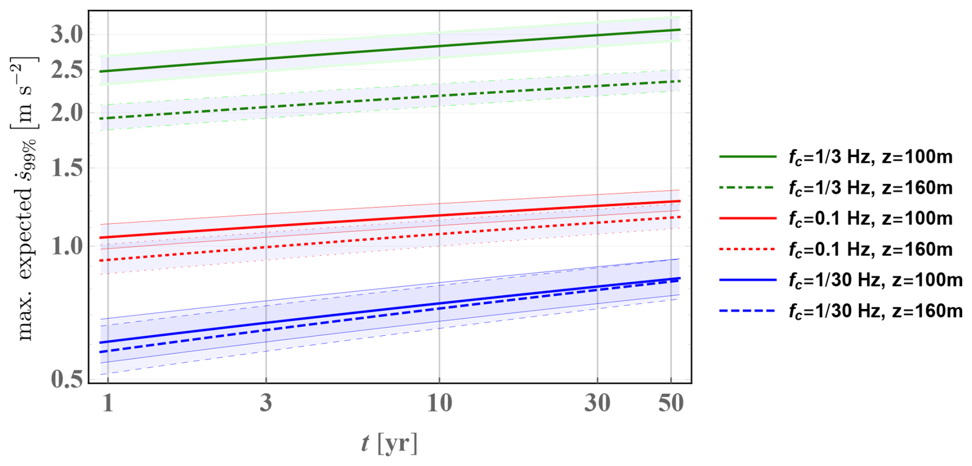
Figure 15 Expected ${\dot{s}}_{\mathrm{99}}$ per return period t for the three different filter scales considered and two heights analyzed. For each case, thick lines correspond to T_base≃39 min (total time span divided by number of samples); shaded areas and thin lines around each case show the range for base periods varying from 10 to 119 min (see text for explanation).

To demonstrate the largest-possible variation due to the definition of the base period T₀, Fig. 15 also shows bands around each line, which may overlap and are thus bounded by thin lines corresponding to the style of each case (e.g., dotted for f_c=0.1 Hz at z = 160 m). The bands show the range of expected extreme ${\dot{s}}_{\mathrm{99}}$ resulting from base periods ranging from 10 min to 119 min, where the latter corresponds to neglect of the directional rate of occurrence. For the shortest response timescale (highest filter scale, $f_{\mathrm{c}}=\mathrm{1}/\mathrm{3}$ Hz), we see a variation of about ±6 % for 50-year ${\dot{s}}_{\mathrm{99}}$, but note that this is the upper limit of uncertainty expected due to base-period representativity. One sees quite dramatically that higher f_c (shorter turbine reaction timescales) give significantly larger 99th-percentile flow accelerations, by more than a factor of 2 when comparing f_s of $\mathrm{1}/\mathrm{3}$ Hz and $\mathrm{1}/\mathrm{10}$ Hz. Further, a larger difference is seen between z = 100 m and z = 160 m for $f_{\mathrm{s}}=\mathrm{1}/\mathrm{3}$ Hz compared to slower response times (higher f_c), with stronger ${\dot{s}}_{\mathrm{99}}$ at z = 100 m due to significant accelerations having a characteristic size of roughly 30–50 m; more analysis needs to be done at higher z to determine if this trend reverses.

We remind the reader that the expected extreme acceleration in Fig. 15 corresponds to the range of wind speeds (8–18 m s⁻¹) at the two heights (z = 100 m, 160 m) considered; there was no apparent dependence on wind speed, as shown in Fig. 5, although the largest ${\dot{s}}_{\mathrm{99}}$ occurred for $\mathrm{10}<U\lesssim \mathrm{15}$ m s⁻¹, which coincides with the most common 10 min mean wind speeds observed around the long-term mean (at 100 m the most common speed was 9.6 m s⁻¹, the mean was 10.6 m s⁻¹, the CDF at 15 m s⁻¹ was 0.83). We do not calculate the contours of expected 50-year $P\left({\dot{s}}_{\mathrm{99}},U\right)$ due to not yet having analyzed cases below 8 m s⁻¹ or above 18 m s⁻¹ and because the directional limitations of this coastal site limited the overall number of offshore winds sampled; this causes difficulty fitting conditional extreme distributions and larger uncertainty relative to finding the marginal distribution. A larger offshore dataset would be needed to make such two-dimensional 50-year contours.

4 Discussion and conclusions

From all low-pass-filtered 10 min ${\dot{s}}_{\mathrm{99}}$ found for offshore flow over a 17-year period at the coastal Høvsøre site, the largest flow acceleration values observed correspond to events having durations longer than the reciprocal of the filter scales chosen ($f_{\mathrm{c}}^{-\mathrm{1}}$). These are long enough to significantly affect wind turbine loads for turbines with characteristic controller/response times of $f_{\mathrm{c}}^{-\mathrm{1}}$ (or shorter) if the transverse spatial scales of the flow structures are sufficiently large. Invoking Taylor's hypothesis to get a crude estimate, the streamwise length scales would be on the order of the product of mean speed and duration, giving gust widths of ∼ 25–35 m for $f_{\mathrm{c}}^{-\mathrm{1}}$ = 3 s and beyond 250 m for $f_{\mathrm{c}}^{-\mathrm{1}}$ = 30 s; for roughly isotropic disturbances, assuming the transverse extent is similar, this is easily large enough to affect conventional turbine blades and associated thrust-based loads. Further, for some extreme acceleration-inducing flow mechanisms, such as cold-front passage or breaking gravity waves associated with the capping inversion, one expects the transverse extent to be much longer than the streamwise one. Larger ${\dot{s}}_{\mathrm{99}}$ tend to correspond to shorter event durations, with larger-amplitude ${\dot{s}}_{\mathrm{99}}$ associated with higher f_c (faster turbine response); this implies length scales roughly as small as the minimum gust widths noted above. Thus for typical offshore turbine blade lengths (> ∼ 50 m) for effective turbine response times of $f_{\mathrm{c}}^{-\mathrm{1}}=\mathrm{3}$ s, the shortest effect of extreme gusts on loads could be mitigated somewhat (e.g., as in load shedding approaching rated speed via a fast controller) or could possibly induce larger blade loads (e.g., flap-wise bending moments) due to a single blade being impacted.

It is remarkable that the growth of wind turbines in recent years – both hub heights and blade lengths – has not only led to offshore turbine loads becoming increasingly impacted by upper-ABL phenomena (more so than surface-induced turbulence), but also led to the character and type of relevant extreme events changing, due in part to the different physical scales of extreme transients above the marine surface layer. Also notable is the variety of diverse signatures exhibited by the extreme acceleration events at 100 and 160 m heights. The events identified indicate both turbulent and nonturbulent flow regimes, including some associated with the stable capping inversion above shallow ABLs; the latter include phenomena such as breaking gravity waves, wave turbulence, entrainment outbreaks, and top-down intrusions, while we also noted extremes associated with frontal passages and other phenomena that have limited association with the ABL top (e.g., borders between strong coherent structures).

For the offshore flow considered at Høvsøre, statistically, stronger filtered acceleration values were found at 100 m height compared to 160 m across all wind speeds and including the extremes. One might expect interaction with the sea surface to be responsible for this, but the most extreme events are not generally turbulent, especially for f_c ≤ $\mathrm{1}/\mathrm{10}$ Hz; for $f_{\mathrm{c}}=\mathrm{1}/\mathrm{3}$ Hz, some (more) turbulence is seen, implying that at higher f_c (faster response times), the surface may have more impact. The effect of the strip of land between the mast and the ocean is also irrelevant at these heights, as choosing to analyze speeds above 8 m s⁻¹ also removes significantly unstable conditions (which could otherwise cause ground effects via mixing). Further investigation at more offshore sites and heights can help clarify this aspect. Although speeds from ∼ 6 to 8 m s⁻¹ are moderately common, 10 min mean wind speeds below 8 m s⁻¹ were ignored because transients at lower speeds (further from rated speed) generally have less impact on loads (Dimitrov et al., 2018; Kelly et al., 2021) and to avoid the coastal effects in unstable conditions; this is further justified by our finding that extreme acceleration values for U ≲ 11 m s⁻¹ are appreciably smaller than those with U ≳ 11 m s⁻¹ (Fig. 5), while mean speeds between 8 ≲ U ≲ 11 m s⁻¹ occur more frequently than those above 11 m s⁻¹. If we included lower speeds and a dependence of extreme ${\dot{s}}_{\mathrm{99}}$ decreasing at smaller U, then using the marginal extreme distribution and associated statistical extrapolation (Fig. 15) would give lower predictions of extreme acceleration at mean wind speeds below ∼ 11 m s⁻¹. No U dependence was found for extremes approaching the high end of the speeds analyzed (18 m s⁻¹, again from Fig. 5), where less impact is expected from the transient acceleration due to it being above rated speed; although shut-down cases could be considered for comparison with the IEC 61400-1, a larger amount of data would be needed to investigate these due to the relative rarity of speeds crossing above the cut-out (around 25 m s⁻¹).

We have assumed that the (westerly) conditions analyzed are representative of all directions offshore, but the significant southeasterly winds that sometimes occur in the spring at Høvsøre (Peña et al., 2016) could conceivably be different enough to have a small impact on the statistics; however, such wind directions are even less common offshore in the North Sea and North Atlantic wind climates characterized by the measurements (e.g., Hahmann et al., 2022). We can get a further sense of the limited potential impact on 50-year extreme accelerations when considering the error lines in Fig. 15, which represent neglect of the fraction of speeds not considered and the fraction of winds coming from offshore.

This work has produced statistics for dominant flow accelerations detected using three different low-pass-filter frequencies f_c (as proxies for characteristic turbine response times), but even more utility could be obtained by characterizing the systematic effect of low-pass filtering on extreme acceleration statistics, i.e., finding an explicit dependence of the extreme ${\dot{s}}_{\mathrm{99}}$ distribution on f_c. Attempts were made to this end but were not included because no simple relation was found to fit the data. Scaling ${\dot{s}}_{\mathrm{99}}$ by $f_{\mathrm{c}}^{-\mathrm{0.6}}$ collapsed the most extreme filtered acceleration amplitudes (with SF < 10⁻⁴ in Fig. 4) to a single curve for both $f_{\mathrm{c}}=\left\{\mathrm{1}/\mathrm{3},\mathrm{1}/\mathrm{30}\right\}$ Hz at z = 100 m and $f_{\mathrm{c}}=\left\{\mathrm{1}/\mathrm{3},\mathrm{1}/\mathrm{10}\right\}$ Hz at z = 160 m (not shown), but no f_c scaling can collapse the extreme distributions or survival functions for all three filter frequencies. This is not surprising: again, most of the extreme events are not simply due to inertial-range turbulence (which permits simple scaling) or any single phenomenon, although we note that more turbulence is observed at 100 m than at 160 m during extreme events. The relative rates of occurrence and relative variation in the strength of the phenomena causing extreme load-driving accelerations are seen to depend on not only f_c but also the distance to both the ground and the capping inversion, as well as the capping inversion strength (Pedersen et al., 2014; Kelly et al., 2019).

A method was developed for use in Monte Carlo aeroelastic simulations (Appendix B) to employ the extreme distributions of offshore filtered accelerations derived above. Practical stochastic expressions are given to relate the magnitude and duration (gust rise time) of filtered flow accelerations including rise time distributions, applicable within the IEC 61400-9 (Zhang et al., 2023) or as a probabilistic supplement (replacement) for the EOG prescription found in the IEC 61400-1; we note that these practical expressions followed from earlier wind speed ramp acceleration studies, and the exact constants and forms may be improved by further investigation and analysis. Additionally considering the IEC 61400-1, its EOG prescription has an implicit rise time of almost 3 s, and for contemporary wind turbines in the highest turbulence subclass (A+) around rated speed, it implies characteristic event acceleration magnitudes that are similar to the 50-year values obtained from measurements at 100–160 m heights with f_c = $\mathrm{1}/\mathrm{3}$ Hz. For higher V_hub, the IEC EOG prescription gives larger acceleration than the 50-year ${\dot{s}}_{\mathrm{99}}$ found here from 100 to 160 m observations with f_c = $\mathrm{1}/\mathrm{3}$ Hz (even for different turbulence subclasses), and ${\dot{s}}_{\mathrm{EOG}}$ are generally larger than 50-year ${\dot{s}}_{\mathrm{99}}$ from measurements with f_c = 0.1 or $\mathrm{1}/\mathrm{30}$ Hz; the lowest turbulence subclass (I_u=12 %) gives weaker accelerations than 50-year ${\dot{s}}_{\mathrm{99}}{|}_{f_{\mathrm{c}}=\mathrm{1}/\mathrm{3}\mathrm{Hz}}$ for speeds below the rated speed (Appendix B). We note that the IEC 61400-1 standard – due to its original basis onshore and with z_hub closer to the surface – prescribes its EOG in terms of turbulence intensity, which is not realistic for offshore turbines with typical hub heights beyond 100 m; as we have seen, load-driving flow accelerations do not follow 10 min standard deviations of wind speed or velocity.

We remind the reader that the results and conclusions herein are for offshore wind; over land, the dominance and effect of turbulence extends further from the surface, typically beyond hub height (e.g., Alcayaga, 2017).

Outlook and continuing work

Continuing work includes further translation to probabilistic gust definitions for the IEC standards, whereby joint distributions of extreme flow accelerations and associated rise times (or magnitude of speed increase) facilitate an update of the extreme operating gust (EOG) in the 61400-1, as well as prescriptions supporting Monte Carlo aeroelastic simulations for the 61400-9. From the acceleration statistics found here, we derived an offshore probabilistic gust prescription towards the IEC 61400-9 standard, as given in Appendix B. More explicit systematic quantification of the durations associated with extreme flow accelerations, with rise time statistics conditioned on wind speed and amplitude (analogous to that for ramps by Kelly et al., 2021), is still ongoing; this should also be done for more offshore sites and heights. One aspect involves the relationship between extreme flow acceleration amplitudes and gust duration. Following ramp studies and preliminary analysis, here we have taken extreme events to have $t_{\mathrm{d}}\propto \mathrm{1}/{\dot{s}}_{\mathrm{99}}$ in a statistical sense, with $\mathrm{\Delta }s\propto {\dot{s}}_{\mathrm{99}}{t}_{\mathrm{d}}$; although such events are due to different phenomena beyond turbulence, a physical hypothesis is that these extreme acceleration events are (mostly) attributable to the passage of a border between coherent flow structures, with the fluid equations of motion and conservation of mass limiting Δs and causing the inverse relation between extreme ${\dot{s}}_{\mathrm{99}}$ and duration. More investigation is needed to explicitly determine the joint behavior of extreme ${\dot{s}}_{\mathrm{99}}$ and the associated {t_d,Δs}, along with the extent to which the border-zone width and advection speed determine the largest acceleration magnitudes. A related aim is to more directly measure the characteristic length scales and orientations of extreme flow acceleration events through both mast-based anemometers and lidar, including more multipoint measurement statistics to characterize the associated flow structure(s). Doing so permits better modeling of transient forces on turbine blades and rotors through constrained aeroelastic simulations incorporating the multidimensional length-scale information.

Starting with single-point statistics, further work could help quantify the behavior and joint distributions of {u,s} for the most common conditions at heights of interest offshore (above the surface layer). Although we found here that extreme acceleration events have ${\dot{s}}_{\mathrm{99}}\simeq {\dot{u}}_{\mathrm{99}}$ while for the most commonly occurring conditions ${\dot{s}}_{\mathrm{99}}\propto {\mathit{\sigma }}_s$, in the latter case we cannot definitively state the degree to which ${\dot{u}}_{\mathrm{99}}\propto {\mathit{\sigma }}_u$ yet, although we do expect it to be so. Classic turbulence theory gives ideal relations between {σ_uσ_vσ_w}, and for fatigue loads, the IEC 61400-1 uses them in its prescriptions; however, the use of measured σ_s in place of σ_u has not been directly addressed, although it might be implicitly accounted for within the empirical constants used in the standard. Further, while theoretical forms are also available relating $\left\{{\mathit{\sigma }}_{\mathrm{d}s/\mathrm{d}t},{\mathit{\sigma }}_s,{\mathit{\sigma }}_{\mathrm{d}u/\mathrm{d}t},{\mathit{\sigma }}_u\right\}$, they do not necessarily apply for the nonideal flow structures that are behind the relationships between $\left\{{\dot{s}}_{\mathrm{99}},{\mathit{\sigma }}_s,{\dot{u}}_{\mathrm{99}},{\mathit{\sigma }}_u\right\}$ and thus fatigue loads. However, this has likely been approximately accounted for in effect by the IEC's empirical description using P₉₀(σ_u); we do note that the latter does not deal with the tails of the PDF from each 10 min period, in contrast to long-term statistics of ${\dot{s}}_{\mathrm{99}}$ or ${\dot{u}}_{\mathrm{99}}$. But the behavior of commonly occurring ${\dot{s}}_{\mathrm{99}}$ may not be markedly different than that of σ_u in terms of its effect on fatigue loads, which is what Fig. 6 appears to imply; although this remains to be directly shown from observations, we expect the flow acceleration paradigm to be more important for extremes.

On the meteorological side, remaining work includes matching flow regimes and conditions to the observed extreme events via analysis of mesoscale model output (e.g., the Weather Research and Forecasting model, WRF) and extended observational data; this also includes exploration of ABL depths, whose observed values can differ from mesoscale model predictions. Such work allows for the investigation of the flow mechanisms and meteorological phenomena that cause extreme flow accelerations offshore. It is also worth noting that microscale models such as large-eddy simulations (LES) are not expected to replicate extreme events like those observed – due to the need to know and simulate details such as the varying strength and structure of capping inversions, as well as variable mesoscale forcings. Coupled models such as WRF-LES might be able to reproduce some of the phenomena; however, the relative rates of occurrence of the various phenomena producing extreme flow accelerations, and the fidelity of simulation of such transients, are unknown, and follow after the non-trivial analysis of matching flow regimes to observed conditions.

Furthermore, the response of different turbines and controllers to extreme accelerations should be examined. For example, at some speeds, certain wind turbines may not be as affected by large accelerations as much as other turbines (depending on the duration and physical extent of the flow disturbance), in a way that is more complicated than is captured by accelerations identified through simple low-pass filtering via f_c. It is possible that more representative filters (e.g., bandpass) can be made to find acceleration statistics based on common control strategies near rated power and that other parameters (e.g., pitch angle) need to be considered. The analysis presented herein, as well as the ongoing work just mentioned, also needs to be expanded to speeds across the full range of wind turbine operation (beyond 8–18 m s⁻¹), to heights above 160 m, and to multiple offshore (and potentially onshore) sites. Lastly, a mean speed dependence has not yet been found or incorporated into the extreme flow acceleration statistics, but with more measurements, this might be elucidated.

Appendix A: Method for estimation of Mann-model parameters from cup and vane measurements

Only wind speed and direction data at 100 and 160 m were available from cup anemometers and vanes for most of the observational period, without three-dimensional velocity component data. Due to this, to facilitate the use of extreme acceleration time series (whether observed as in Sect. 3 or synthesized as in Appendix B), it was necessary to create a method to practically derive Mann-model turbulence parameters from such measurements for use in constrained gust simulations – as created by McWilliam et al. (2023b) based on the time series described in Sect. 3. Such a method for finding turbulence parameters without vertical velocity components is also useful because two-dimensional cup/vane instrumentation or floating lidar¹⁹ is standard for industrial wind energy preconstruction measurement campaigns.

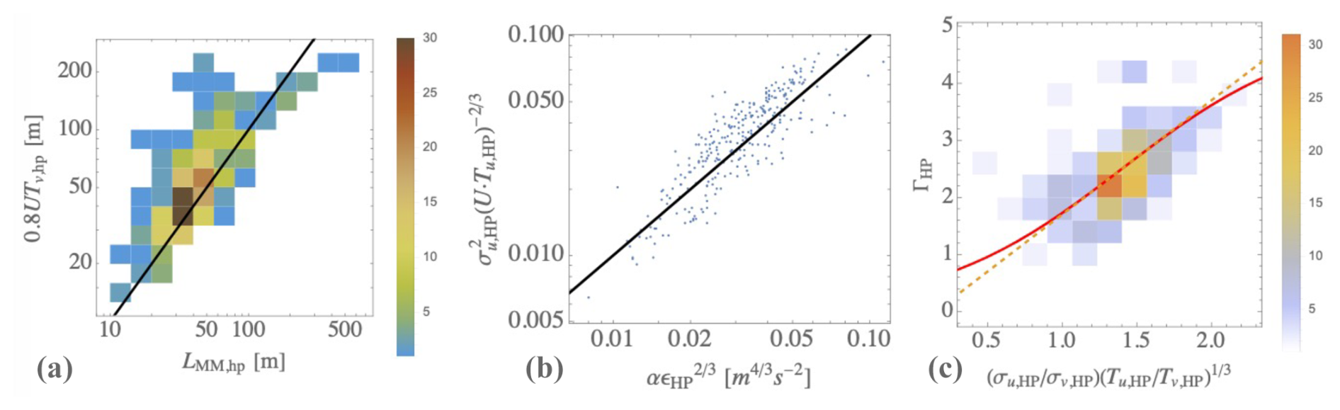
Figure A1 Estimates versus spectrally fit values of Mann-model parameters for spatially high-pass-filtered ($f_{\mathrm{HP}}=U/\mathrm{2}$ km) turbulence behind the extreme acceleration events. (a) Length scale, with 1 : 1 indicated by the black line. (b) Amplitude parameter $\mathit{\alpha }{\mathit{ϵ}}^{\mathrm{2}/\mathrm{3}}$, again with a black 1 : 1 line. (c) Anisotropy parameter Γ, with Eq. (A2) as a solid line and its linear equivalent as a dashed line. Colors in the joint PDFs indicate the event count, showing how the estimate is covering the most commonly observed values.

Although Kelly (2018) found the Mann-model turbulence length scale to be expressible in terms of shear through the bulk relation $L_{\mathrm{M}}\approx {\mathit{\sigma }}_s/(\mathrm{\Delta }U/\mathrm{\Delta }z)$, this stems from turbulence dominated by shear production, which is not the case for the flow behind many extreme acceleration events; furthermore, we wish to address vertical inhomogeneity (variation in shear and turbulence) and allow the use of time series from different heights for constrained turbulence simulations that embed acceleration events. We are thus challenged to diagnose the length scale using two-dimensional (horizontal) information at individual heights in a way that matches measured spectra from three-dimensional sonic anemometers.

Based on the limited three-dimensional sonic anemometer measurements available at 100 and 160 m and independent sonic measurements from the shorter mast at 80 m height, one-dimensional frequency spectra (and thus streamwise wavenumber spectra via Taylor's hypothesis) of uu, uw, vv, and uw were calculated for the 10 most extreme acceleration events per wind speed bin identified at each location. These allowed χ² fits to the single-point velocity spectral tensor Φ_ij (Mann, 1994; IEC, 2019), which give the three Mann-model turbulence parameters ($L_{\mathrm{M}},\mathit{\alpha }{\mathit{ϵ}}^{\mathrm{2}/\mathrm{3}},\mathrm{\Gamma }$) that allow synthesis of turbulence time series following the 61400-1 standard (IEC, 2019). The flow during extreme events exhibited significant nonstationarity due to mesoscale (low-wavenumber) variance, which is not well-represented by Mann-model spectra²⁰, so the turbulence with each event was also found from fits to spatially high-pass filtered spectra using Taylor's hypothesis and a second-order Butterworth filter with $f_{\mathrm{hp}}=U/\left(\mathrm{2}\mathrm{km}\right)$. From the raw and high-pass-filtered three-dimensional velocity time series, it was found that the turbulence length scale could be estimated most simply using the integral timescale of lateral velocity fluctuations: the raw signal (i.e., including nonstationarity) gave $L_{\mathrm{M}}\approx \mathrm{0.5}{L}_v\simeq \mathrm{0.5}{T}_{v}U$, while the high-pass-filtered turbulence had $L_{\mathrm{M},\mathrm{hp}}\approx \mathrm{0.8}{T}_{v,\mathrm{hp}}U$, where the integral timescale is calculated through temporal autocorrelation and the subscript hp denotes spatially high-pass-filtered turbulence. The L_M, hp estimates are much better than unfiltered L_M, with Fig. A1 displaying joint PDFs of estimated versus observed (spectrally fit) L_M, hp over the collection of extreme acceleration events. One can see some scatter in the estimates, but we note that the acceleration (gust) description is the focus of constrained simulations, and the background turbulence length scale is secondary. We further remind the reader that explicit calculation of the length- and timescales associated with extreme accelerations is ongoing/future work.

Analogous to obtaining L_M, it was found that the Mann-model amplitude parameter can also be estimated using the integral timescale. Knowing that $\mathit{\alpha }{\mathit{ϵ}}^{\mathrm{2}/\mathrm{3}}$ scales as ${\mathit{\sigma }}_u^{\mathrm{2}}{L}^{\mathrm{2}/\mathrm{3}}$ (Mann, 1994; Kelly, 2018), from the fits to the spatially high-pass-filtered spectral tensor components (again with $f_{\mathrm{hp}}=U/\mathrm{2}$ km), we find that

$$\begin{array}{}\text{(A1)}& \mathit{\alpha }{\mathit{ϵ}}^{\mathrm{2}/\mathrm{3}}\simeq {\mathit{\sigma }}_{u,\mathrm{hp}}^{\mathrm{2}}{\left(T_{u,\mathrm{hp}}U\right)}^{-\mathrm{2}/\mathrm{3}}\end{array}$$

matches the three-dimensional spectrally fit values well and note that $\mathit{\alpha }{\mathit{ϵ}}^{\mathrm{2}/\mathrm{3}}\approx \mathrm{0.7}{\mathit{\sigma }}_{u,\mathrm{hp}}^{\mathrm{2}}{\left(T_{v,\mathrm{hp}}U\right)}^{-\mathrm{2}/\mathrm{3}}$ also gives a crude estimate. The estimate from Eq. (A1) versus spectrally fit $\mathit{\alpha }{\mathit{ϵ}}^{\mathrm{2}/\mathrm{3}}$ is shown in the center plot of Fig. A1 for the extreme acceleration events.

Lastly, we find a form to estimate for the anisotropy (eddy-lifetime) parameter Γ, which we expect to be proportional to $(T_u/T_v{)}^{\mathrm{1}/\mathrm{3}}$ and ${\mathit{\sigma }}_u/{\mathit{\sigma }}_v$ from Kelly (2018); we find that the most common values follow ${\mathrm{\Gamma }}_{\mathrm{hp}}\approx \left[\mathrm{2}\left(\frac{{\mathit{\sigma }}_{u,\mathrm{hp}}}{{\mathit{\sigma }}_{v,\mathrm{hp}}}\right){\left(\frac{T_{u,\mathrm{hp}}}{T_{v,\mathrm{hp}}}\right)}^{\mathrm{1}/\mathrm{3}}-\mathrm{0.3}\right]$, whereas keeping the mesoscale fluctuations (not high-pass spatial filtering or de-trending) degrades the fits and leaves little discernible pattern for estimation of Γ in terms of the unfiltered quantities that we measure. Because Γ cannot be negative and is limited to Γ≤5 (Mann, 1994), a practical form to estimate it is

$$\begin{array}{}\text{(A2)}& {\mathrm{\Gamma }}_{\mathrm{hp}}\approx \mathrm{2.5}\left\{\mathrm{1}+\tanh \left[\mathrm{0.8}\left({\displaystyle \frac{{\mathit{\sigma }}_{u,\mathrm{hp}}}{{\mathit{\sigma }}_{v,\mathrm{hp}}}}{\left({\displaystyle \frac{T_{u,\mathrm{hp}}}{T_{v,\mathrm{hp}}}}\right)}^{\mathrm{1}/\mathrm{3}}-\mathrm{1.4}\right)\right]\right\};\end{array}$$

this is shown in the right-hand plot of Fig. A1, superimposed on the joint PDF of $\left({\mathit{\sigma }}_{u,\mathrm{hp}}/{\mathit{\sigma }}_{v,\mathrm{hp}}\right){\left(T_{u,\mathrm{hp}}/T_{v,\mathrm{hp}}\right)}^{\mathrm{1}/\mathrm{3}}$ and Γ from Mann-model fits to spectra of {uu, uw, vv, uw}.

Appendix B: Use of extreme acceleration distribution for gust synthesis and simulation

To investigate the effects on turbine loads and probabilistic design (e.g., via Monte Carlo simulation), it is useful to be able to “convert” the extreme acceleration statistics into gusts for simulation as a probabilistic alternative to (or augmentation of) the IEC 61400-1 standard's extreme operating gust (EOG). On average, the expected duration or rise time for a given streamwise extreme flow acceleration, denoted by T_d, tends to decrease with acceleration amplitude. This has been documented in wind ramp studies (Hannesdóttir et al., 2019; Hannesdóttir and Kelly, 2019; Kelly et al., 2021), with the latter showing rise times to be inversely proportional to acceleration; plotting the joint distribution $P\left(T_{\mathrm{d}},\mathrm{\Delta }s/\mathrm{\Delta }t\right)$ from the data of Kelly et al. (2021), as in Fig. B1, we more clearly see that $T_{\mathrm{d}}\approx \left(\mathrm{6}\mathrm{m}{\mathrm{s}}^{-\mathrm{1}}\right)/\left(\mathrm{\Delta }s/\mathrm{\Delta }t\right)$ for ramps.

One could adapt this for extreme accelerations ${\dot{s}}_{\mathrm{e}}$ having durations larger than a given filter timescale $f_{\mathrm{c}}^{-\mathrm{1}}$; however, we observe that less extreme acceleration events do not necessarily have such long durations²¹ and that such a simple expression would always give the same wind speed increase of $T_{\mathrm{d}}{\dot{s}}_{\mathrm{e}}=\mathrm{6}$ m s⁻¹. From preliminary analysis of the strongest events, for practicality we extend $T_{\mathrm{d}}\approx \left(\mathrm{6}\mathrm{m}{\mathrm{s}}^{-\mathrm{1}}\right)/{\dot{s}}_{\mathrm{e}}=\mathrm{\Delta }{s}_{\mathrm{ref}}/{\dot{s}}_{\mathrm{e}}$ to suggest the form

$$\begin{array}{}\text{(B1)}& T_{\mathrm{d}}\left({\dot{s}}_{\mathrm{e}}\right)\simeq {\displaystyle \frac{\mathrm{\Delta }{s}_{\mathrm{ref}}/a_{\mathrm{ref}}}{{\left[\mathrm{1}+{\left({\dot{s}}_{\mathrm{e}}/a_{\mathrm{ref}}\right)}^{\mathit{\xi }}\right]}^{\mathrm{1}/\mathit{\xi }}}};\end{array}$$

here a_ref≃0.4 m s⁻² is the value below which the durations are shorter than $\mathrm{\Delta }{s}_{\mathrm{ref}}/{\dot{s}}_{\mathrm{e}}$, with $T_{\mathrm{d}}\to \mathrm{\Delta }{s}_{\mathrm{ref}}/{\dot{s}}_{\mathrm{e}}$ for extreme accelerations ${\dot{s}}_{\mathrm{e}}>a_{\mathrm{ref}}$. The coefficient ξ=3 was found empirically along with a_ref, and we note that the parameters in Eq. (B1) could be refined through ongoing work, wherein the timescales of extreme acceleration events are investigated in detail.

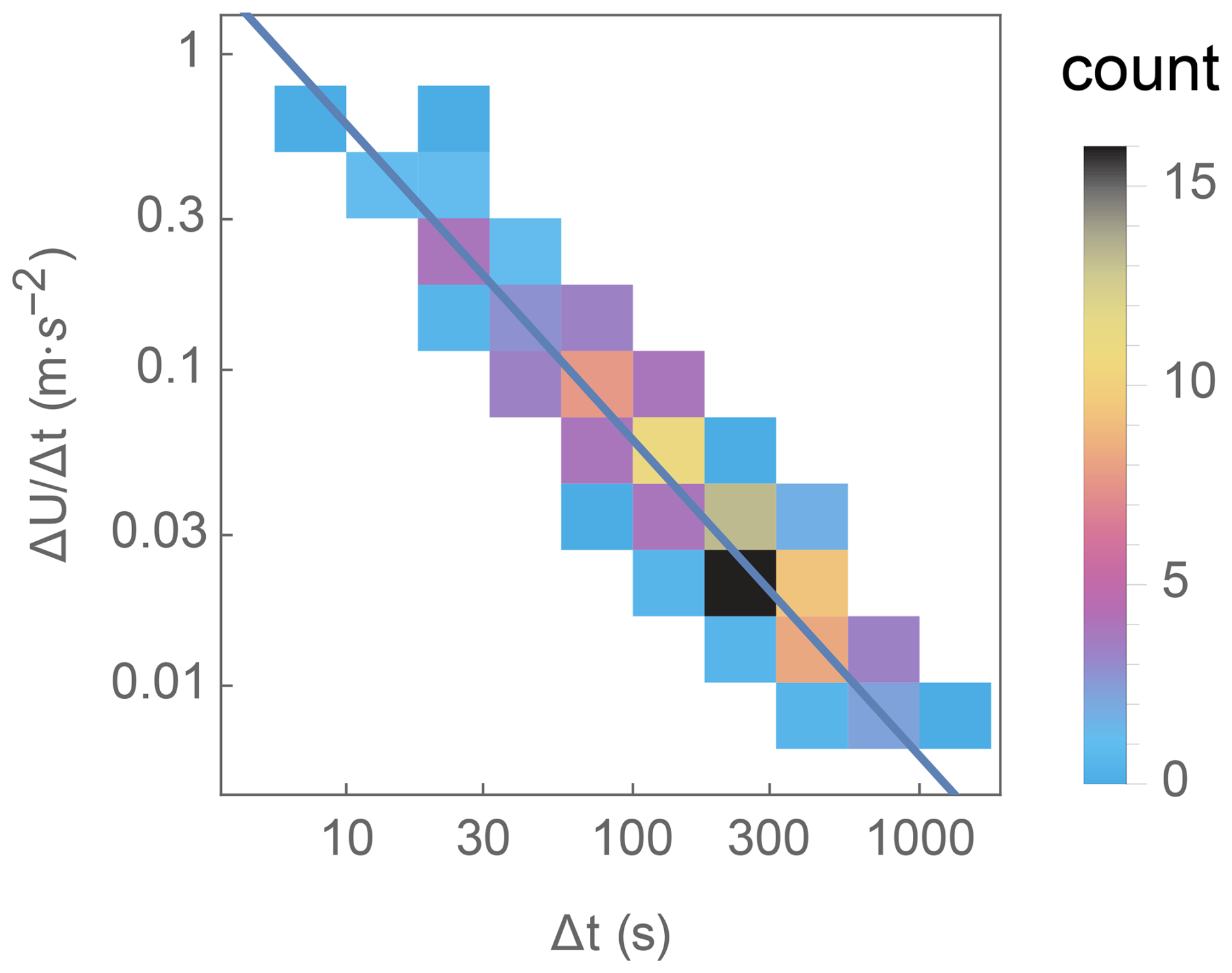
Figure B1 Joint PDF of bulk acceleration and rise times from the ramp data of Kelly et al. (2021). The solid line is (6 m s⁻¹) $/$ Δt.

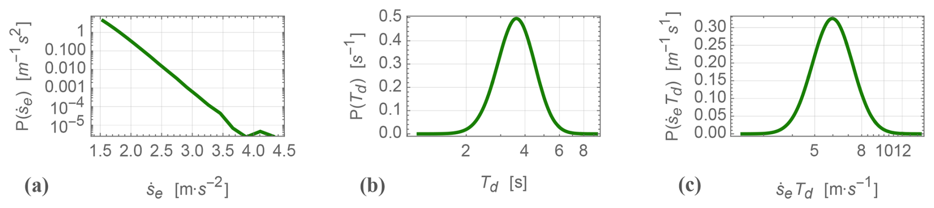
Figure B2 Example distributions of extreme acceleration (a), event duration (b), and the associated wind speed jump (c) synthesized for simulation; the $P\left({\dot{s}}_{\mathrm{e}}\right)$ used corresponds to $f_{\mathrm{c}}=\mathrm{1}/\mathrm{3}$ Hz at a height of 100 m.

The T_d from Eq. (B1) needs to be perturbed to give a distribution of rise times, $P\left(T_{\mathrm{d}}|{\dot{s}}_{\mathrm{e}}\right)$, again to avoid $T_{\mathrm{d}}{\dot{s}}_{\mathrm{e}}$ being fixed at 6 m s⁻¹ for extreme ${\dot{s}}_{\mathrm{e}}$. The deterministic expression (B1) can be scaled stochastically by a factor following the dimensionless log-normal distribution

$$\begin{array}{}\text{(B2)}& {\displaystyle \frac{\mathrm{1}}{w\sqrt{\mathrm{2}\mathit{\pi }}}}\cdot \exp \left\{-{\displaystyle \frac{\mathrm{1}}{\mathrm{2}}}\left[w^{\mathrm{2}}+{\left({\displaystyle \frac{\ln x}{w}}\right)}^{\mathrm{2}}\right]\right\},\end{array}$$

where the dimensionless width w is small relative to 1; to begin, we assume it is independent of ${\dot{s}}_{\mathrm{e}}$. An example of the distributions $P\left({\dot{s}}_{\mathrm{e}}\right)$, P(T_d), and $P\left({\dot{s}}_{\mathrm{e}}{T}_{\mathrm{d}}\right)$ with w=0.2, synthesized using 4×10⁶ random values of ${\dot{s}}_{\mathrm{e}}>\mathrm{0.5}$ m s⁻² following $P\left({\dot{s}}_{\mathrm{e}}\right)$ from the observed statistics at z = 100 m and f_c = $\mathrm{1}/\mathrm{3}$ Hz, is shown in Fig. B2. The actual width w and its potential dependence on acceleration ${\dot{s}}_{\mathrm{e}}$ (or wind speed) are the subject of future work.

Synthesized pairs of $\left\{{\dot{s}}_{\mathrm{e}},T_{\mathrm{d}}\right\}$ can be used to drive a stochastic gust prescription (for, e.g., aeroelastic simulations), given an analytical form for the gust. While the IEC 61400-1 standard has a deterministic gust, we propose a stochastic version that simply follows from the load-inducing increase in wind speed due to extreme flow acceleration and its statistics:

$$\begin{array}{}\text{(B3)}& s\left(t\right)=U+{\dot{s}}_{\mathrm{e}}{\displaystyle \frac{T_{\mathrm{d}}}{\mathit{\pi }}}\left\{\mathrm{1}+\tanh \left[{\displaystyle \frac{\mathit{\pi }\left(t-t_{\mathrm{c}}\right)}{T_{\mathrm{d}}}}\right]\right\},\end{array}$$

where again the mean speed is U, and t_c is the time corresponding to the peak acceleration (i.e., when $s={\dot{s}}_{\mathrm{e}}$). This has been formulated to give the simple acceleration waveform $\dot{s}\left(t\right)={\dot{s}}_{\mathrm{e}}\mathrm{sech}\left[\mathit{\pi }\left(t-t_{\mathrm{c}}\right)/T_{\mathrm{d}}\right]$ and to allow convenient use of extreme ${\dot{s}}_{\mathrm{99}}$ distributions (such as $P\left({\dot{s}}_{\mathrm{e}}\right)$ given above) and comparison with or extension of the standard EOG. The IEC standard prescribes $s_{\mathrm{EOG}}\left(t\right)=U+\mathrm{0.37}{V}_{\mathrm{gust}}\sin \left(\mathrm{3}\mathit{\pi }t/T_{\mathrm{EOG}}\right)\left[\cos \left(\mathrm{2}\mathit{\pi }t/T_{\mathrm{EOG}}\right)-\mathrm{1}\right]$, with a total duration of T_EOG=10.5 s and magnitude V_gust; it implies a maximum acceleration ${\dot{s}}_{\mathrm{e},\mathrm{EOG}}=V_{\mathrm{gust}}/\left(\mathrm{1.71}\mathrm{s}\right)$ that occurs at $t_{\mathrm{c}}=\mathrm{0.378}{T}_{\mathrm{EOG}}\simeq \mathrm{4}$ s. For illustration and comparison, the extreme gust perturbations from the mean speed normalized by the maximum acceleration, $s^{\prime }\left(t\right)/{\dot{s}}_{\mathrm{e}}\equiv \left[s\right(t)-U]/{\dot{s}}_{\mathrm{e}}$, are given in Fig. B3 for the IEC's EOG, along with the stochastic form Eq. (B3). The latter is shown using three different values of rise time, $T_{\mathrm{d}}=\mathit{\{}\mathrm{1.71},\mathrm{4},\mathrm{6}\mathit{\}}$ s, corresponding to short, common, and long T_d from the P(T_d) shown in Fig. B3; accompanying these normalized wind speed gusts are the corresponding $\dot{s}\left(t\right)$, also normalized by ${\dot{s}}_{\mathrm{e}}$.

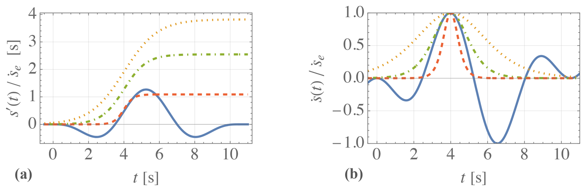
Figure B3 Wind speed gust function (a) and its time derivative (b) normalized by the peak acceleration EOG from IEC 61400-1.

From the left-hand plot of Fig. B3, we see that one can replicate the positively accelerating segment of s_EOG(t) using Eq. (B3), with $T_{\mathrm{d}}=V_{\mathrm{gust}}/{\dot{s}}_{\mathrm{EOG}}\left(t_{\mathrm{c}}\right)=\mathrm{1.71}$ s and consequently ${\dot{s}}_{\mathrm{e},\mathrm{EOG}}=V_{\mathrm{gust}}/\left(\mathrm{1.71}\mathrm{s}\right)$, or generically, ${\dot{s}}_{\mathrm{e}}{T}_{\mathrm{d}}=\mathrm{\Delta }s$; for longer rise times, one then sees larger wind speed jumps for a given acceleration ${\dot{s}}_{\mathrm{e}}$.

For multi-megawatt turbine hub heights (z_hub>60 m) and rotor diameters (D>z_hub), we also see that the IEC's form for V_gust is determined by its second term, expressible as ${\dot{s}}_{\mathrm{e},\mathrm{EOG}}=\frac{I_{\mathrm{ref}}\left(\mathrm{10.8}\mathrm{m}{\mathrm{s}}^{-\mathrm{2}}+V_{\mathrm{hub}}/\mathrm{0.69}\mathrm{s}\right)}{\mathrm{1}+\mathrm{0.1}D/\mathrm{42}\mathrm{m}}$ where I_ref corresponds to the IEC turbine intensity subclass, while the hub-height wind speed is V_hub; the IEC 61400-1 implies EOG peak acceleration varying linearly from 2.2 to 3.6 m s⁻² for I_ref of 12 % (class C) and from 3.3 to 5.5 m s⁻² for I_ref of 18 % (class A+). This peak EOG acceleration can exceed the 50-year amplitudes extrapolated from measurements by a factor of 2 for f_c = $\mathrm{1}/\mathrm{3}$ s and by even larger factors for lower f_c (Fig. 15); however, we see that the rising part (positive acceleration) of the EOG waveform, which lasts for 2.79 s (from t = 2.46 to 5.25 s), has an average equal to $\mathrm{0.62}{\dot{s}}_{\mathrm{e},\mathrm{EOG}}$. For I_u = 18 %, and V_hub ranging from 8 to 18 m s⁻¹, then $\mathrm{0.62}{\dot{s}}_{\mathrm{e},\mathrm{EOG}}$ ranges from 2 to 3.4 m s⁻²; for $\mathrm{10}\lesssim V_{\mathrm{hub}}\lesssim \mathrm{16}$ m s⁻¹, this falls between the 50-year values of ${\dot{s}}_{\mathrm{e}}{|}_{f_{\mathrm{c}}=\mathrm{1}/\mathrm{3}\mathrm{Hz}}$ statistically extrapolated from measurements at 100 and 160 m heights. Thus the IEC 61400-1 EOG prescription and its inherent rise time of 2.79 s for wind speeds near rated imply an event-mean acceleration consistent with 50-year values extrapolated from measurements when considering the strongest turbulence subclass (A+, 18 %). For lower IEC turbulence subclasses, the EOG-implied event acceleration corresponds to lower f_c; we point out that the IEC standard's prescription was originally developed onshore and closer to the ground, basically assuming that gusts are turbulent.

We remind the reader that Eq. (B3) is meant to synthesize extreme acceleration time series for many different values of both ${\dot{s}}_{\mathrm{e}}$ and T_d, as shown in the distributions of Fig. B2; McWilliam et al. (2023b) did such a synthesis, applying it through constrained turbulence simulations, for use in ultimate load calculations.