Load case selection for finite-element simulations of wind turbine pitch bearings and hubs

Finite-element simulations of large rolling bearings and structural parts are an indispensable tool in the design of wind turbines. Unlike simpler structures or smaller bearings in rigid environments where analytical formulas suffice, wind turbine components require a more comprehensive approach. This is because analytical formulas often fall short in predicting load distributions and stresses, leading to inadequate designs. However, due to the complexity of the finite-element models and number of operational load cases involved, it is necessary to strike a balance between achieving realistic results and keeping computational times manageable. This study focuses on the selection of load cases for simulations of pitch bearings and hubs of wind turbines. The models for these contain the hub, the pitch bearings, the inner parts of three blades, and any necessary interface parts. The simulation results allow for the calculation of static and fatigue strength. Given the complexity of the problem, with each rotor blade having 6 degrees of freedom, 5 types of loads, and a pitch angle, their potential combinations would result in an unmanageably high number of required simulations. The present work assumes that binning of 1 or more degrees of freedom into sufficiently small bins results in the other degrees of freedom showing negligible variation. Defining the values for these binned degrees of freedom thus gives the values for the others and reduces the number of combinations drastically. The validity of this approach is verified by the standard deviations of the unbinned degrees of freedom and by exemplary stress calculations of a pitch bearing ring. The blade's azimuth angle and bending moments of one blade root allow determining the loads at all three blade roots and thus the derivation of stress time series with 384 simulations of a full rotor with a reasonable degree of confidence.

1 Introduction

Pitch bearings of wind turbines are slewing bearings which connect each rotor blade with the rotor hub (Hau, 2017). There are several commercially available design types for these bearings, as listed in Stammler (2020). Bearings can fail for various reasons, as described in ISO 15243 (ISO, 2017). Rolling contact fatigue and structural fatigue of the rings are among these reasons and are driven by stress cycles. Hubs are the structural centerpiece of wind turbine rotors, providing the linkage between the three blades and the turbine's drive train. Similar to the pitch bearing ring, the structural integrity of hubs is influenced by stress cycles, which drive fatigue (Hau, 2017).

Aero-elastic simulations of wind turbines provide the load time series at various positions, such as the rotor blade roots (Burton et al., 2011; Hau, 2017). In order to assess the lifespan of individual components, it is necessary to establish a relationship between the applied loads and the resulting stresses. This involves calculating the nonlinear dependencies between these variables. Finite-element (FE) simulations derive these relations for each calculated load case. In theory it is possible to use FE simulations with the loads at each discrete time step of the input data. This approach would yield time series data of stresses, which could then be utilized for analytical fatigue calculations. Menck et al. (2020) state a duration of 25 min for one simulation of a model containing one rotor blade and bearing. Based on this, hundreds of thousands of load cases for a full rotor would result in several years of computational time on a similar machine. Doing so is not possible within reasonable computing times, and a reduction in load cases for the simulations is therefore necessary.

Aside from the definition of load cases, the selection of a model type is another crucial aspect for a FE simulation. This study covers full rotors with three blades. The load and stress distributions of pitch bearings and hubs are influenced by the loads the three rotor blades transfer to their roots. It is assumed that the stress distribution in one pitch bearing is influenced by the loads of the other pitch bearings by load transfer through the hub.

Chen and Wen (2012) simulated a double-row four-point contact ball bearing that is used as a pitch bearing in a 1.5 MW wind turbine. They used a model with three rotor blade roots but did not elucidate on the selection of load cases.

To the best of the authors' knowledge, the only approaches for load case selection published in the literature are limited to the determination of load cases for one blade root, i.e., one pitch bearing:

• Characterize and simplify the input load time series by means of rain flow counts, and use the reduced data to define load cases for the FE. Use the results, which again have the form of rain flow count results, to calculate fatigue.

• Use the extreme operating loads. Evenly spread load steps in between those, and calculate the results for these load cases. Interpolate between the results to obtain stress time series and apply rain flow counts to calculate fatigue.

Both approaches will result in inaccurate results in comparison to FE simulations of each time step of the input data. The extent of the inaccuracies depends on the number of load cases simulated and the turbine configuration.

Becker et al. (2017) describe a process as per the first of the abovementioned approaches where the input load time series are first processed into rain flow counts, which then give the load cases for the FE simulations. To account for the complex behavior of large bearings, the bearing circumference is split into several sections, with rain flow counts done for each. Stammler et al. (2018) did 126 simulations with a rotor of a 3 MW turbine with variations in pitch angles and bending moments. They evaluated the load distribution in one pitch bearing and kept the pitch angles and the loads of the other bearings at one-third of the loads of the primary bearing constant. They did not elucidate on the reasons for the load case selection. The load distribution in the pitch bearing was shown to be dependent on the interfaces. Menck et al. (2020) used one-third of a rotor with rotational symmetric boundary conditions to reduce the computational effort in comparison to a full rotor. They ran 358 simulations on this model and varied the pitch angle and the resulting bending moment and its angle as per the second approach. With a regression of the resultant rolling body loads, they obtained time series of rolling body loads and calculated the fatigue life of the bearing raceways. In particular for comparably weak hub structures, Becker and Jorgensen (2023) stated the need for full-rotor simulations for pitch bearing damage modes, which are driven by the edgewise loads of the blades. They also point to the need for taking into account flapwise moments and combinations of the individual moments for comprehensive assessments.

Figure 1 Flowchart of load case selection with preceding rain flow count.

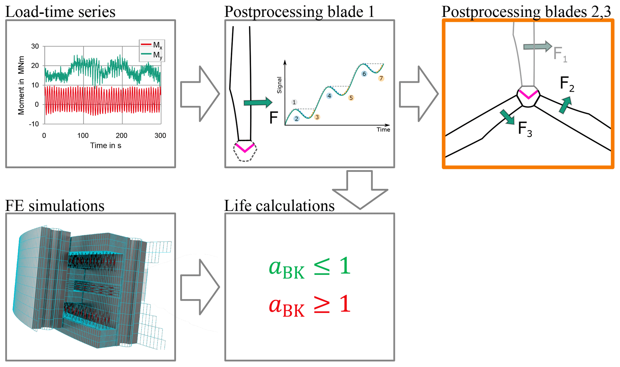
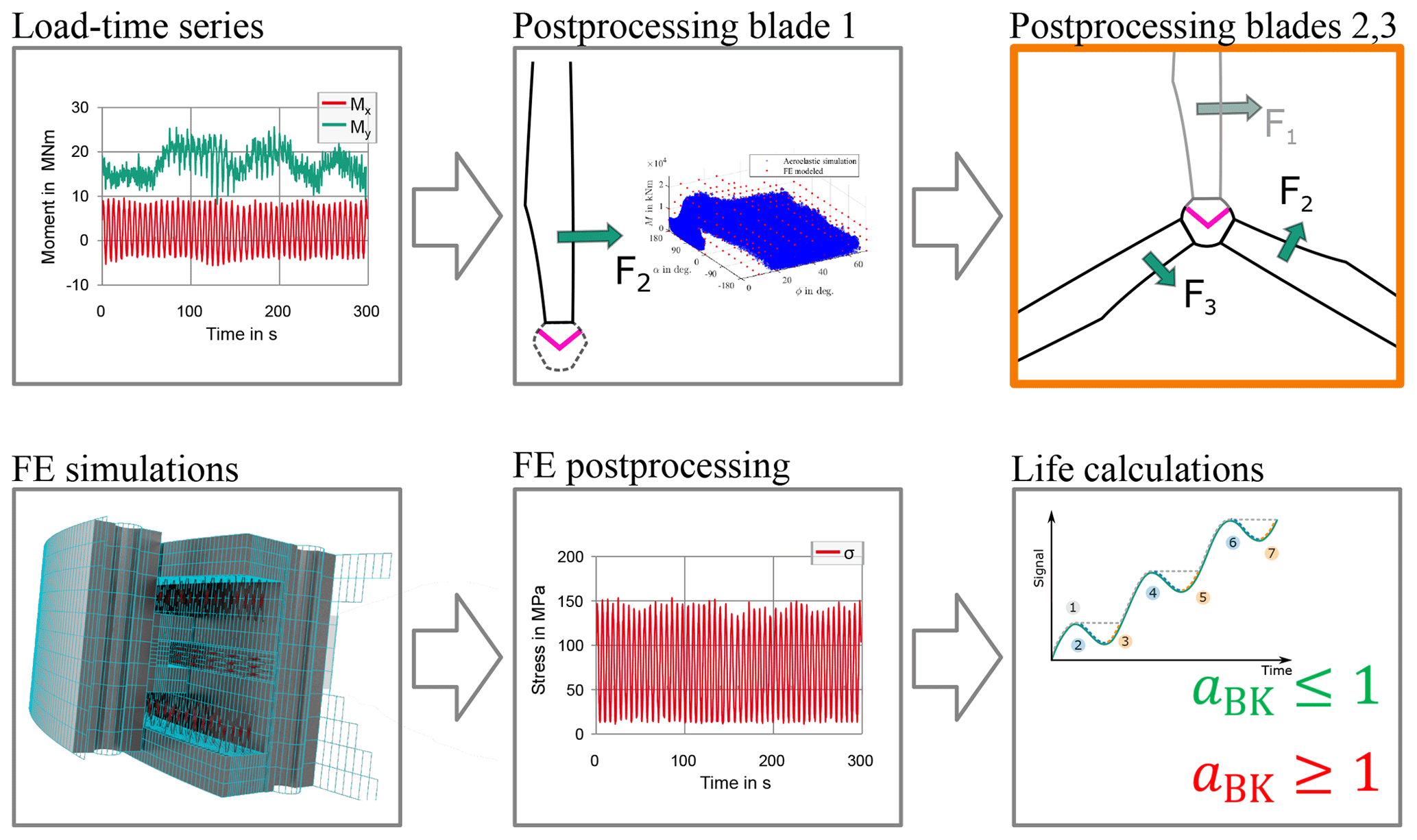
Figure 2 Flowchart of load case selection with preceding interpolation and stress time series creation.

Figures 1 and 2 summarize the two published approaches as flowcharts. Figure 1 depicts the approach by Becker et al. (2017). The input load time series (upper-left box) are processed by rain flow counts of the loads of an arbitrarily selected blade one (upper-center box). These are then used for finite-element simulations of the pitch bearings and their interfaces (lower-left box). As the load cases are already given in the form of rain flow counts, the FE results can be used directly for fatigue calculations. The FKM guideline contains methods for such calculations (lower-center box; FKM, 2021). Becker (2024a) apply the FKM guideline for static and fatigue bearing ring strength. The selection of the loads of the other blades (upper-right box in orange) is not explained in the abovementioned publications.

Figure 2 depicts the approach by Stammler et al. (2018) and Menck et al. (2020). The input loads (upper-left box) are processed and evaluated to obtain the ranges of each load component. In between the extreme values, a grid of load cases is created (upper-center box). These grids are then used for finite-element simulations of the pitch bearings and their interfaces (lower-left box). The results need additional postprocessing by interpolation to obtain stress time series (lower-center box). A rain flow count of these time series is then used for fatigue calculations (lower-right box). The selection of the loads of the other blades (upper-right box in orange) is either omitted or not explained in detail in the abovementioned publications.

To the authors' knowledge, there is a notable gap in the existing literature regarding a comprehensive exploration of load case selection specifically for pitch bearing simulations involving three rotor blades, highlighted by the orange boxes in Figs. 1 and 2. Furthermore, there appears to be a lack of published works addressing load case selection for rotor hubs. The central inquiry driving this study is to understand to which extent the loads of one rotor blade bearing are correlated with or affected by the loads of the other blade bearings or the rotor position.

The remainder of this article begins with Sect. 2, which introduces definitions for the following sections, the necessary data input, and the methods which are applied to determine dependencies. The data input for the case studies includes aero-elastic simulation time series of the IWT7.5-164 reference turbine and three commercial turbines. Section 3 covers the results of the case studies and shows which relationships are useful for the load case selection. The final discussion and conclusions then summarize the findings of this work.

2 Definitions and methods

2.1 Coordinate systems

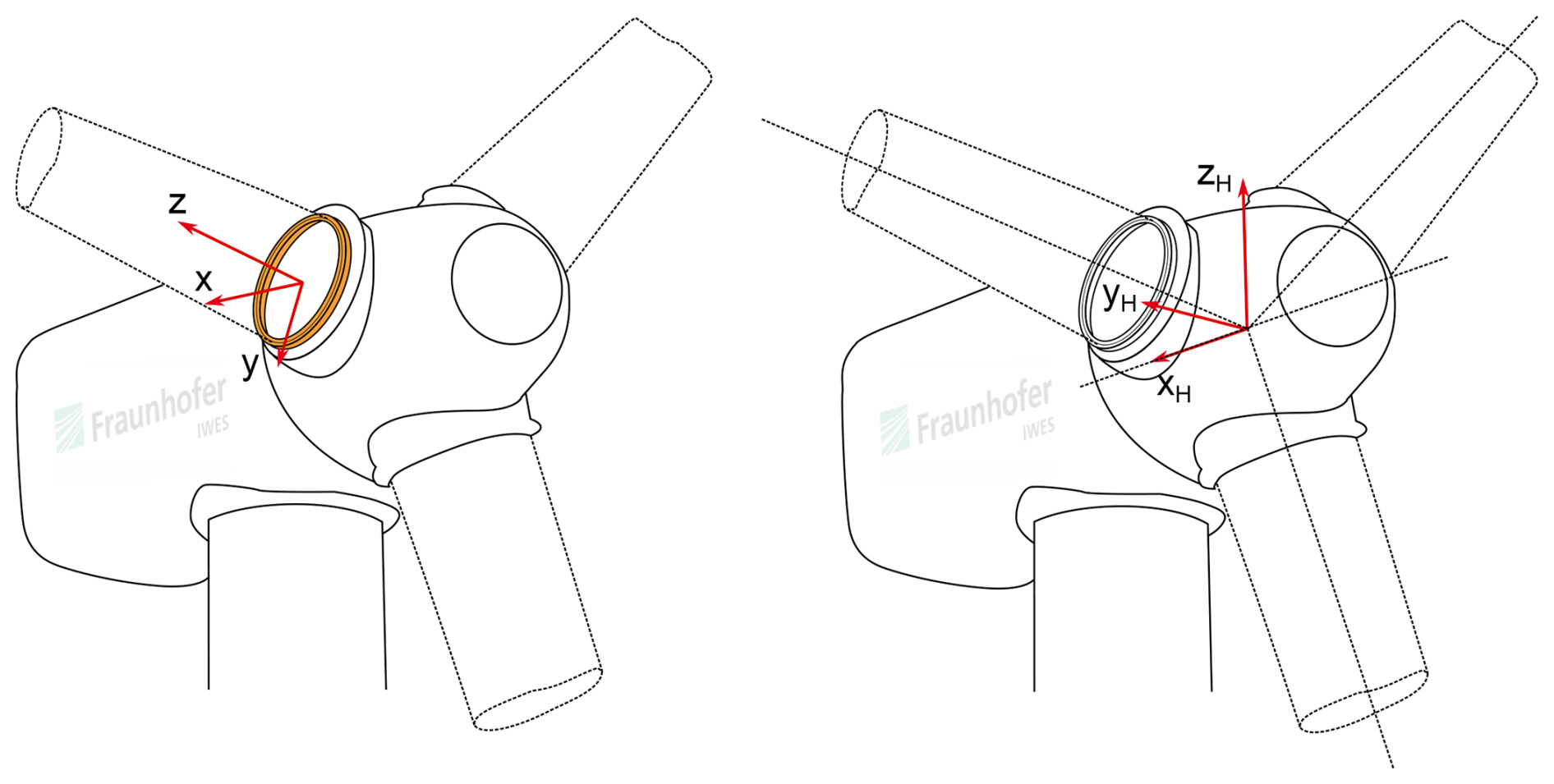
Pitch bearing loads in this study use the Cartesian coordinate system shown in Fig. 3 (left), with the exception of the pitch angle θ, which is positive in the clockwise direction, i.e., opposite to the right-hand rule. This convention is the industry standard, and most turbine simulation time series follow it. Although the coordinate system does not rotate with the pitch angle, the term flapwise bending moment refers to M_y,B and the term edgewise bending moment to M_x,B in the following. Strictly speaking, M_y,B is only a pure flapwise moment if the pitch is at 0°. Flapwise bending moments are the result of wind thrust, whereas edgewise bending moments are mostly dominated by gravitational forces. Hub center loads and blade azimuth angles in this study use the coordinate system shown in Fig. 3 (right).

Figure 3 Pitch bearing coordinate system (fixed to rotor hub, left); hub coordinate system (right) (Stammler, 2020).

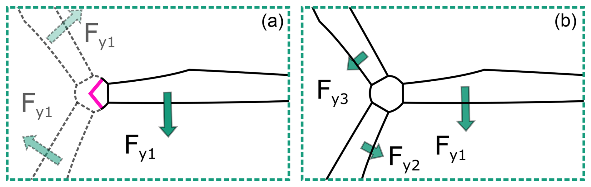
The blade azimuth angle Φ_r,B is defined in Fig. 4. Note that the 0° position is arbitrarily chosen. As long as it is consistent throughout the data set, any other position can serve as 0°.

Figure 4 Blade azimuth angle Φ_r,B.

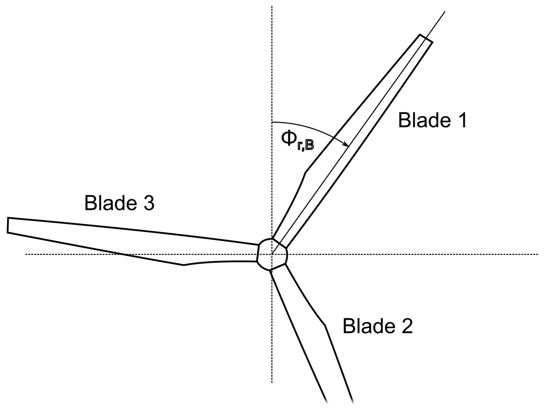
The three blades have the arbitrarily chosen numbers one, two, and three, which are consistent throughout the simulation data set. The numbers increase clockwise, as seen from the incoming wind direction. Φ_r,B refers to blade one. In the following, blade one is also called the primary blade, and blades two and three are called secondary blades.

2.2 Input data and signal selection

The time series output of aero-elastic simulations is the input for the present work. Time series output can contain numerous signals. Becker et al. (2017), Stammler et al. (2018), Menck et al. (2020), Becker and Jorgensen (2023), and Becker (2024b) all use the edgewise and flapwise bending moments M_x,B and M_y,B to describe the load cases of one pitch bearing. The use of the combined bending moments M_xy,B and their load angle β is equivalent to the use of M_x,B and M_y,B. Stammler et al. (2018) and Menck et al. (2020) also include the pitch angle θ.

The input data for finite-element simulations with three blades thus need pitch angles θ; blade root bending moments M_x,B and M_y,B; and forces F_x,B, F_y,B, and F_z,B for all three blades. The need for the inclusion of pitch angles is based on the results of Stammler et al. (2018) and Menck et al. (2020), who show the load distribution in a blade bearing to be dependent on the non-rotationally symmetric stiffness profile of the rotor blade. At constant blade root loads, different pitch angles can thus cause different load distributions on its circumference. While the aforementioned signals suffice to build finite-element simulations, the introduction of additional signals for the selection of load cases might render more meaningful relations between the load components. The blade's azimuth angle Φ_r,B and the out-of-plane rotor moment M_y,H are included as additional signals. Φ_r,B is strongly related to the dominant 1p component of all M_x,B values. The out-of-plane rotor moments might help to narrow relations between the individual M_y,B.

2.3 Data binning and mean value evaluation

The relations between different load signals are evaluated with the help of data binning (bin counts). The relation between each time series file duration and the period it represents of the turbine design life is expressed by multipliers. A multiplier quantifies the number of repetitions of each time series file to reach the design life of the turbine. One or more signals are assumed to be independent, and the other signals are assumed to be dependent. For each equidistant bin of the independent signal(s), all assumed dependent signals are evaluated for their mean value and standard deviation. The mean value and standard deviation are weighted by the multipliers. The use of the standard deviation implies the assumption of a normal distribution of the signal values around the mean value, which is not necessarily the case. Yet, it allows for a good comparison between different data binning with different bin numbers.

Table 1 Example output of data binning.

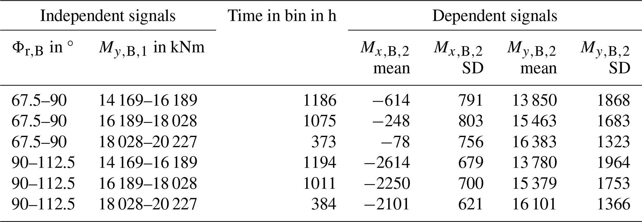
In the case of more than one assumed independent signal, the bin counts are stacked. For each bin of the first signal, all bins of the second signal are counted. Table 1 lists an example structure of such a result for two independent signals and two dependent signals. The values are taken from the later case study but limited to two bins for the first and three bins for the second signal, resulting in a total of six bins. The first signal is Φ_r,B, and the second is signal $M_{y,\mathrm{B},\mathrm{1}}$. The first two columns contain the bin range of these two signals. The third column contains the time spent in the bin within the turbine life. The columns for the dependent signals then contain their mean values (“mean”) and standard deviations (“SDs”). In the context of the present work, the mean values are the input values of the FE simulations for all values of signals one and two in the respective bin range.

The standard deviations of dependent signals are combined by weighted means to a single standard deviation for all bins and normalized against the maximum value of $M_{y,\mathrm{B},\mathrm{1}}$ of the data set. The number of bins of the independent signals is increased until the standard deviation of the dependent signals converges or until a finer resolution of bins is unreasonable.

2.4 Finite-element simulations

The verification of the assumption of cross-influences between the pitch bearings and the load case selection method needs finite-element simulations. This work uses a bearing model as described in Graßmann et al. (2023) in a full-rotor model. A full rotor contains three blades, blade bearings, the hub, part of the main shaft, and all necessary interface parts such as stiffener plates. The bearing model uses nonlinear springs to represent the rolling bodies and connects these via force-distributed constraints to the raceways. The bearing rings including the bolt holes are represented with 3D elements. The hub and all other interfacing steel parts are represent with 3D elements as well. The modeling approach is validated in Graßmann et al. (2023) with experimental results. The deviations between measured and simulated tangential ring deformations are below 10 %. Further validation is not part of the present work. The three blades are modeled according to Menck et al. (2020) with shell elements, except for the root section, which consists of 3D elements. Finite-element simulations within the framework of the present work serve two targets:

• Verify the initial assumption of the influence of secondary blade bearing loads on the stress distribution on blade bearing one (see Sect. 3.2).

• Relate the standard deviation of the data binning for outer loads with deviations of the stress values in the bearings (see Sect. 3.4).

Figure 5 One-third-rotor model (a); full-rotor model (b).

A rotor model which considers only one rotor blade and introduces symmetry conditions on its boundaries is called a one-third-rotor model (see left of Fig. 5). A comparison between the full-rotor and one-third-rotor model results provides the verification of cross-influences of the three blades. As the model for this work was initially set up as a full rotor and only a limited number of simulations are done, one-third-rotor behavior is achieved by loading all three blades with the same load. For convenience, this model is designated as the one-third-rotor model in the following.

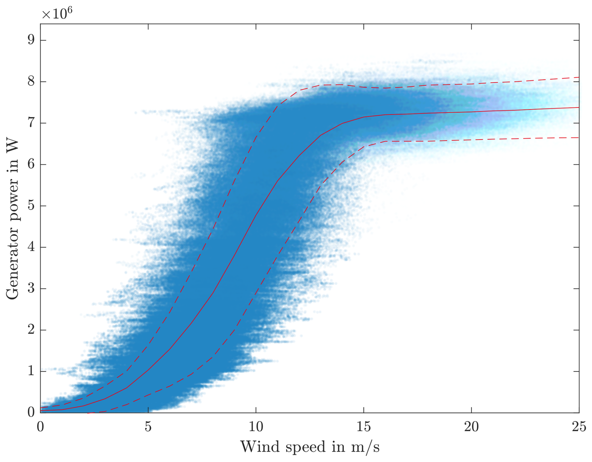
Figure 6 Generator power over wind speed from simulation data set. Red line – mean value, dashed red lines – 95 % quantile.

3 Case studies

3.1 Input data and scenario

The IWT7.5-164 is a nearshore reference wind turbine (Sevinc et al., 2014). The authors used time series data of this turbine in previous works; see Stammler et al. (2019) and Stammler (2020). Table 2 lists the main properties of the turbine. The simulation time series, taken from Requate et al. (2020), contain all the signals listed above, which makes the calculation of additional signals, as described in Sect. A, unnecessary for this case study. The data set comprises 156 files of the DLC1.1 with mean wind speeds from 3 to 25 m s⁻¹. Figure 6 shows the generator output power over momentary wind speed in the x direction of the hub coordinate system of Fig. 3 with calculated mean values.

Table 2 Main characteristics of the IWT7.5-164, from Stammler (2020).

Figure 7 Time series of IWT7.5-164 at 11 m s⁻¹.

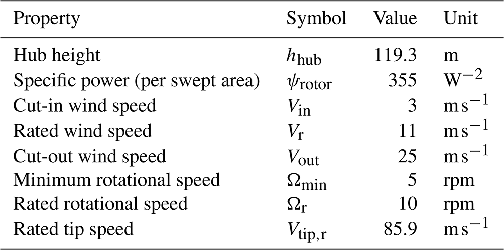
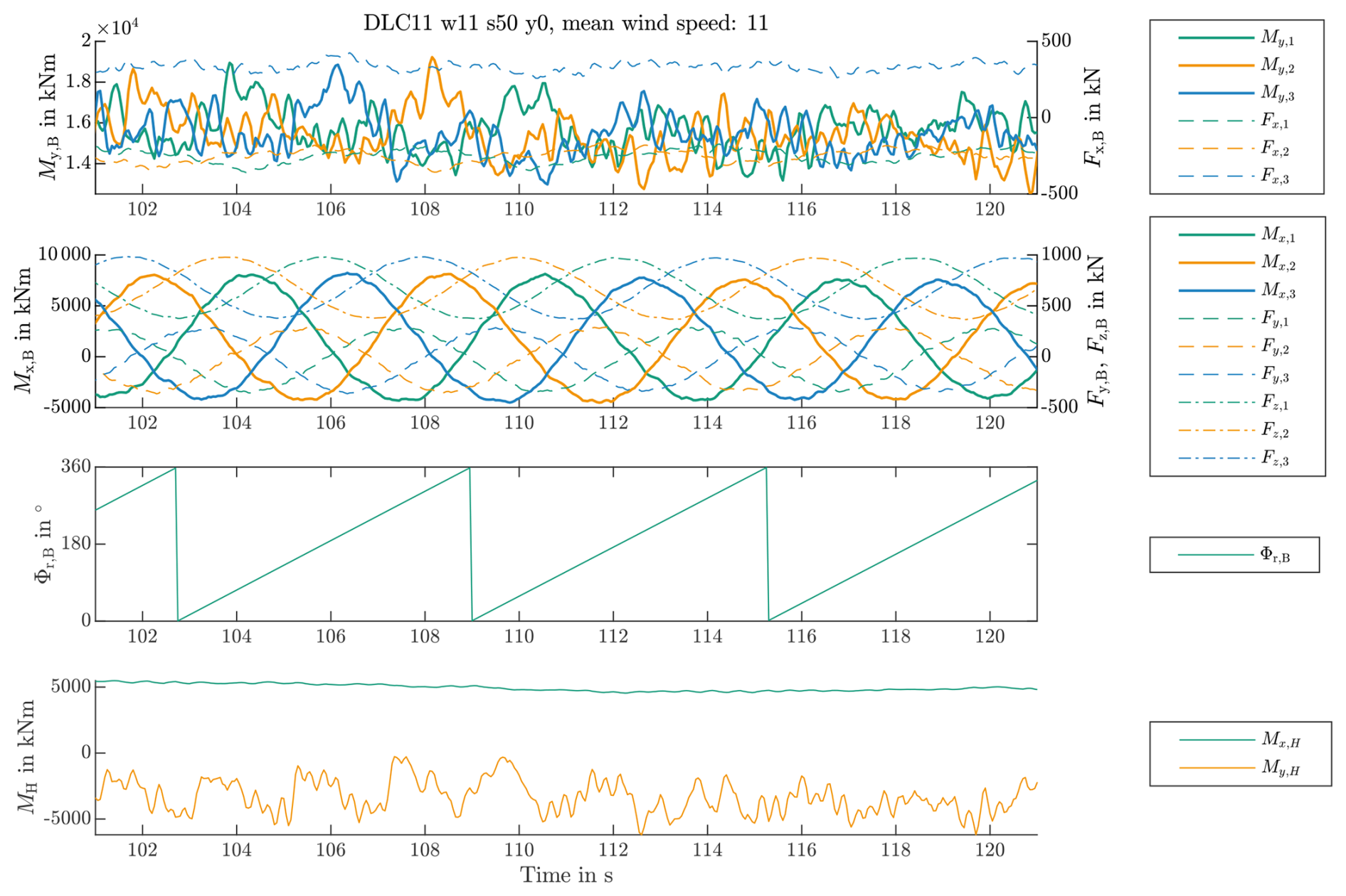
Figure 7 shows an exemplary time series of the turbine simulation data at 11 m s⁻¹ mean wind speed and gives a first impression of the characteristics of the individual signals. The turbine is in power production mode. The top row shows the M_y,B and F_x,B of all three blades, and the next row shows the M_x,B, F_y,B, and F_z,B of all three blades. Signals pertaining to the same blade are displayed in the same color. Bending moments are the thick lines, and forces are the thin and dashed lines. The blade's azimuth angle is depicted in the third row, and the two tilting moments of the rotor, M_y,H (green) and M_z,H (orange), are depicted in the last row. The flapwise blade moments and the rotor moment on its horizontal axis appear more stochastic than the edgewise moments and the connected forces. Edgewise bending moments and radial forces have a sine characteristic with a phase angle shift of 120° between them. Relating these signals either to each other or to the rotor azimuth angle seems to be a promising approach.

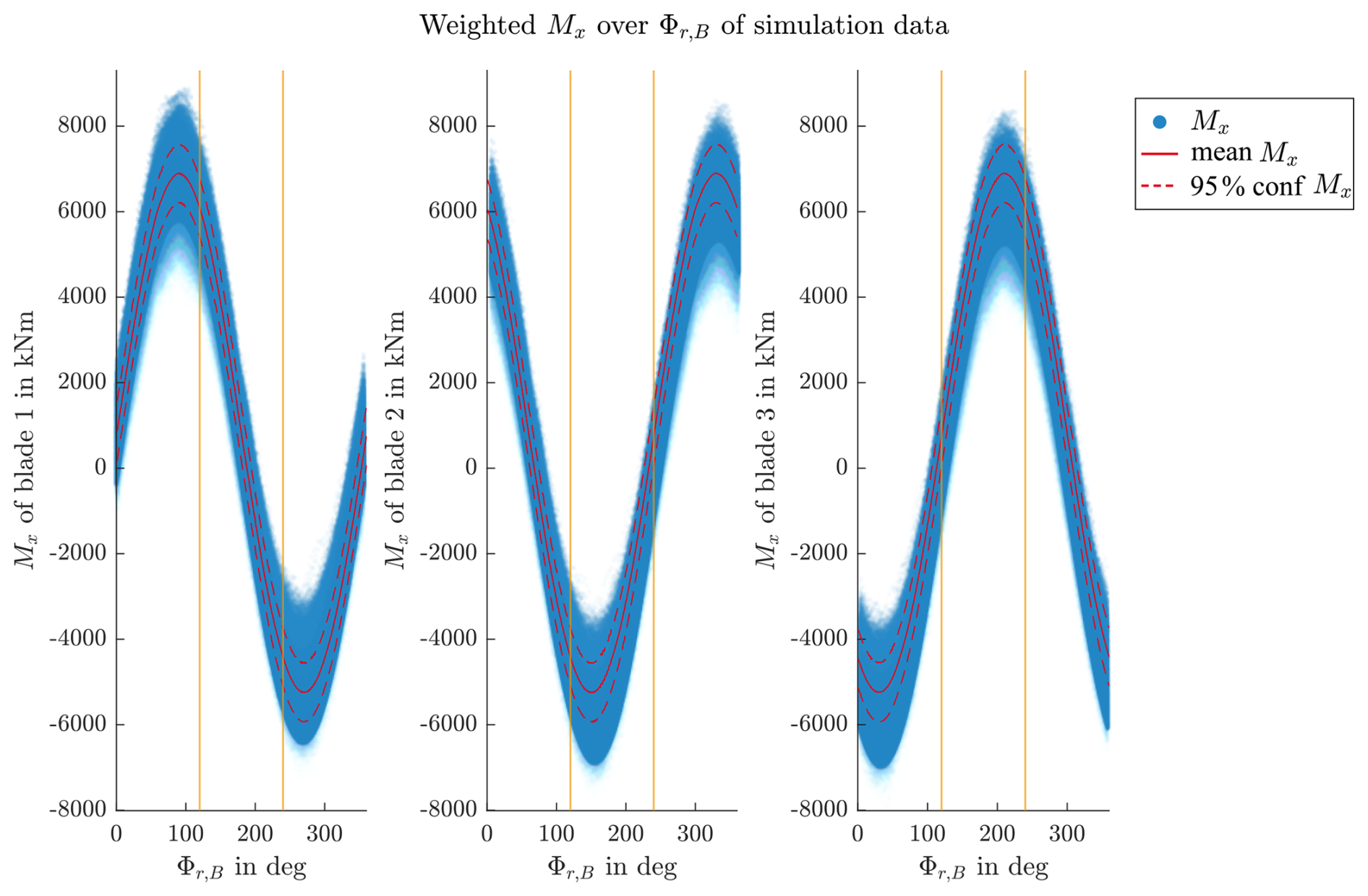
Figure 8 Weighted M_x,B of all blades over Φ_r,B (red line: mean value, dashed red lines: 95 % quantile).

Figure 8 further supports the close relation of Φ_r,B and M_x,B. The blue areas contain all data points of the input data, with the full red line being the mean value and the dashed lines being the boundaries of the 95 % quantile. The vertical orange lines have a 120° spacing and allow for easier visual comparison of the three plots.

In addition to the IWT7.5-164 as a reference turbine, time series of three commercial turbines are part of the case studies. All time series are the result of aero-elastic simulations. The turbines are both onshore and offshore with rated outputs between 2 and 15 MW. The time series include power production load cases from the cut-in to cut-out wind speed of the turbines. The time series were chosen due to their availability. Due to their commercial nature, further details on turbines and loads are subject to confidentiality agreements and cannot be disclosed. In the context of the present work, they serve to confirm the results are not limited to the specific design of the IWT7.5-164.

The finite-element simulations are done with a full-rotor model of one of the commercial turbines. Again, details of the design cannot be disclosed. This rotor model was selected because the structural design of the components is far more detailed than usual in reference turbines, and the authors deemed the obtained results to be closer to state-of-the-art turbines than those achievable with IWT7.5-164 components.

3.2 Finite-element simulation of one rotation

To verify the central assumption of cross-influences between the individual pitch bearing loads, the first set of finite-element simulations comprises one exemplary rotor rotation in 12 steps. This rotation is simulated with a full-rotor and one-third-rotor model.

Stress cycles in the outer ring drive its structural fatigue. Locations with high stress amplitudes and a high number of stress cycles are most prone to fatigue. Their identification is a critical part of the design process and is not within the scope of the present work. Instead, locations with high stress amplitudes are selected and then used for comparative analyses. These locations are the outer-ring bolt holes at two distinct circumferential positions. These are on the positive and negative y axis of the pitch bearing coordinate system and experience high stress dynamics due to the M_x edgewise loads.

The left part of Fig. 9 shows a simulated stress distribution in an outer-ring bolt hole with higher values in red and lower values in blue. The stresses are tangential or hoop stresses. In the case of the outer ring, they are tensile stresses. The right part is a concept sketch of the bearing. The front shows a section with the outer ring on the left and the inner ring on the right. The outer ring attaches to the hub and the inner ring to the blade of the turbine. The shown bearing is a four-point contact ball bearing with a contact angle of 45°. A blade root bending moment such as M_x causes axial loads on the bearing rings. The rolling bodies turn these into a combined radial and axial load, which pushes the outer ring to the outside and the inner ring towards the bearing center. As the inner ring is pushed to the bearing center, it gets compressed. The deformations are usually smaller than on the outer ring, and the compressive stresses are less critical for fatigue. The outer ring, however, experiences tensile hoop stresses and larger deformations. The lower side of the visualization is the hub side of the pitch bearing and usually experiences smaller deformations and stresses than the blade side.

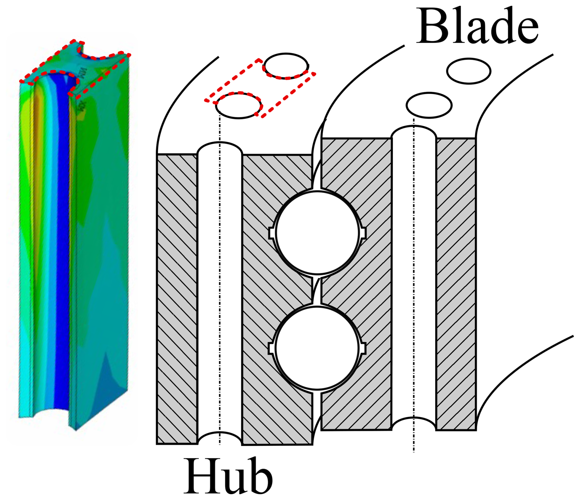
Figure 9 Visualization of tangential stresses in bolt holes of outer ring (left) and location in the bearing (right).

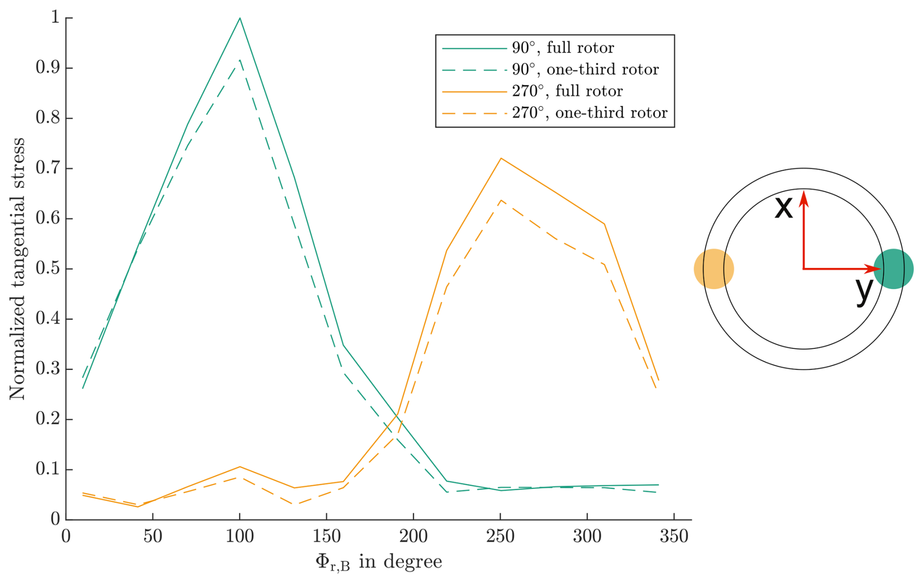
Figure 10 Normalized tangential stresses of bearing outer ring at two positions for full-rotor and one-third-rotor simulations over one rotor revolution.

Figure 10 shows stresses of two outer-ring bolt holes on the positive and negative y axis for a full-rotor and one-third-rotor simulation over one rotor revolution. The circumferential position of the bolts is on the positive and negative y axis of the pitch bearing coordinate system, as indicated in the right part of the figure. The position on the positive y axis is 90°, and the position on the negative y axis is 270°. The results are normalized for the maximum stress at all positions and given as a function of the rotor position. The axial position in the bolt hole, at which the stress values are obtained, is defined as the position at which the maximum stress in the respective bolt hole occurs.

From Fig. 10, the 90° position is identified as the more critical position for fatigue due to its higher stress amplitude. The amplitude of the stress cycle in the bolt hole for the one-third-rotor model is 9.25 % lower than that of the full-rotor model. This results in a significant difference in the outer-ring structural fatigue life and demonstrates the importance of cross-influences of the blade loads. The Φ_r,B azimuthal positions of the extreme stresses are close to those of the extreme $M_{x,\mathrm{B},\mathrm{1}}$ during the rotation. The following simulations thus only use the extreme values of $M_{x,\mathrm{B},\mathrm{1}}$ to obtain stress amplitudes for comparative analyses.

3.3 Data binning results

This section evaluates possible selections of independent signals that define the load cases for finite-element simulations. For each independent signal, increasing numbers of bins are considered. At this point, the decision criterion for the inclusion of a signal as an independent signal in the load case definition is the standard deviation of assumedly dependent signals, with smaller deviations being better. In the following section on verification, this standard deviation is exemplarily related to deviations in stress amplitudes. Due to the large number of potential dependent signals, a full visualization becomes impractical. Therefore, Tables 3–6 present the standard deviations of $M_{x,\mathrm{B},\mathrm{2}}$ and $M_{y,\mathrm{B},\mathrm{2}}$ as representative signals. These are the edgewise and flapwise bending moments of the second blade. All values are normalized to the maximum value of $M_{y,\mathrm{B},\mathrm{1}}$ and also given as a percentage of the standard deviation of the signal in the full data set. The edgewise bending moments are primarily influenced by gravitational forces and thus depend on the blade's azimuth angle Φ_r,B. The initial data binning thus utilizes this azimuth angle. Other potential independent signals include pitch angle, flapwise and edgewise blade bending moments, and rotor moments. For the following analysis, we exclude the rotor moment on the vertical axis, M_z,H, as it remains approximately constant; see Fig. 7.

Table 3 Data binning results for single independent signals.

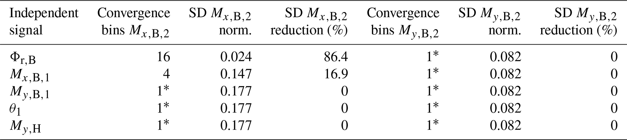
^∗ There is no significant reduction in standard deviations with more bins.

Table 4 Stacked data binning results with 16 bins for Φ_r,B.

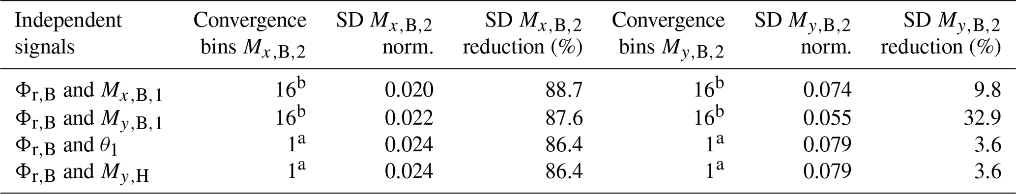
^a There is no significant reduction in standard deviations with more bins. ^b There are small but notable improvements with increasing bins.

Tables 3 to 5 contain the results of the reference turbine. The first column lists the independent signal or signals. In the case of more than one independent signal, the data binning is stacked; i.e., the first signal is sorted into bins, and the second signal is then sorted into bins for each bin of the first. The second and fifth columns list the number of bins for a convergence of the standard deviation of the exemplary dependent signals; i.e., higher bin numbers do not result in a significant further reduction in deviations. The third and sixth columns contain the combined, normalized standard deviation of the dependent signals. The normalization is done with reference to a maximum value of $M_{y,\mathrm{B},\mathrm{1}}$. Finally, columns four and seven show the effect of the data binning in comparison to an unprocessed data set.

Table 5 Combined bin count results with all 16 bins for Φ_r,B and $M_{y,\mathrm{B},\mathrm{1}}$.

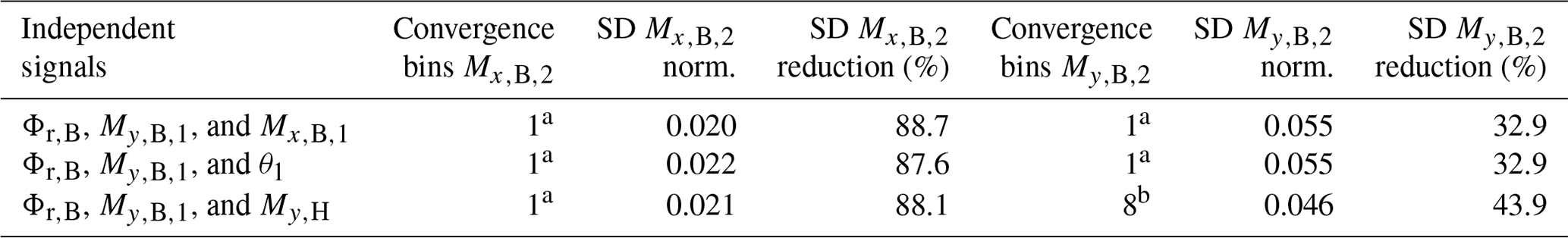
^a There is no significant reduction in standard deviations with more bins. ^b There are small but notable improvements with increasing bins.

Table 3 contains the results for data binning involving a single independent signal. The first line uses Φ_r,B as an independent signal. This is binned into 16 bins, each with a range of 22.5°. The combined standard deviation of $M_{x,\mathrm{B},\mathrm{2}}$ over all bins is 2.4 % of the maximum $M_{y,\mathrm{B},\mathrm{1}}$ in the data set. In comparison to a data set with no binning, this equals a reduction of 86.4 %. However, this binning does not result in a reduction in the standard deviation of $M_{y,\mathrm{B},\mathrm{2}}$.

With the exception of Φ_r,B and $M_{x,\mathrm{B},\mathrm{1}}$ as independent signals, increasing the number of bins did not lead to a reduction in the standard deviation of the dependent signals. Notably, Φ_r,B significantly outperforms $M_{x,\mathrm{B},\mathrm{1}}$ in this regard. It is also worth noting that no discernible relationship could be established between the flapwise bending moments of blade two and any of the signals selected as independent signals. For the following tests with stacked data binning, the number of 16 bins for Φ_r,B is kept constant, and $M_{x,\mathrm{B},\mathrm{1}}$ is omitted.

Table 4 contains the results for stacked data binning, each employing 16 bins for the blade's azimuth angle Φ_r,B as the first independent signal. The columns with the convergence bins refer to the second independent signal. Interestingly, neither the pitch angle nor the out-of-plane rotor moment improved the results. However, when the flapwise and edgewise bending moments were introduced in addition to the azimuth angle, there was a noticeable reduction in the standard deviations of the selected dependent signals.

Both moments had positive effects, with more pronounced effects when the dependent bending moments were in the same direction. For instance, binning the flapwise bending moment reduced the deviation of the flapwise moments at blade two more effectively with 32.9 % compared to the binning of edgewise moments, which led to a reduction by 9.8 %. The differences in the reduction in $M_{x,\mathrm{B},\mathrm{2}}$ are less pronounced. Thus, the next stack of data binning takes the combination of Φ_r,B and $M_{y,\mathrm{B},\mathrm{1}}$ as the first two independent signals.

Table 5 shows the results for stacked bin counts for three independent signals. As 16×16 bins result in 256 bins from the combinations of Φ_r,B and $M_{y,\mathrm{B},\mathrm{1}}$, this evaluation is limited to eight bins as a maximum for the third signal with a focus on the overall number of simulations. The introduction of the pitch angle or the edgewise bending moment did not yield any significant improvements to the deviations. However, the introduction of the rotor moment M_y,H further reduces the standard deviation of $M_{y,\mathrm{B},\mathrm{1}}$.

Table 6 Combined bin count results with varying bins for Φ_r,B and $M_{y,\mathrm{B},\mathrm{1}}$.

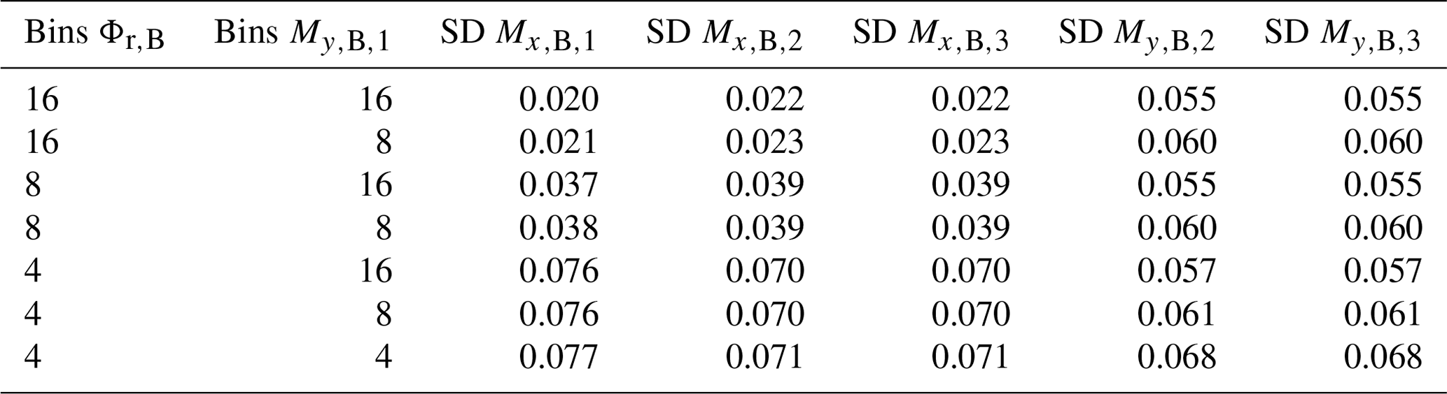
Table 7 Bin count results with all 16 bins for Φ_r,B, $M_{y,\mathrm{B},\mathrm{1}}$, and commercial turbines.

Again with a focus on the overall number of simulations necessary, the following evaluation tries to explore possibilities for bin reductions within the stacked data binning of two independent signals. The stacked binning using Φ_r,B and $M_{y,\mathrm{B},\mathrm{1}}$ has shown promising results. Given that the selection of 16 bins for Φ_r,B is based on its individual bin count, it might be possible to reduce any of the number of bins of the combination. Table 6 shows the results of such bin variations. In contrast to the previous tables, this table contains the results of more dependent signals, again in the form of normalized values. The number of Φ_r,B bins has a larger effect on the deviations of any M_x,B signals than on the M_y,B deviations. Conversely, the number of bins for $M_{y,\mathrm{B},\mathrm{1}}$ has a more pronounced influence on the deviations of other M_y,B signals. Reducing the number of bins within the examined ranges consistently leads to noticeable changes in the deviations. This means the number of bins of any individual signal in the combined data binning cannot be reduced in comparison to binning with single signals without negative influences on the results.

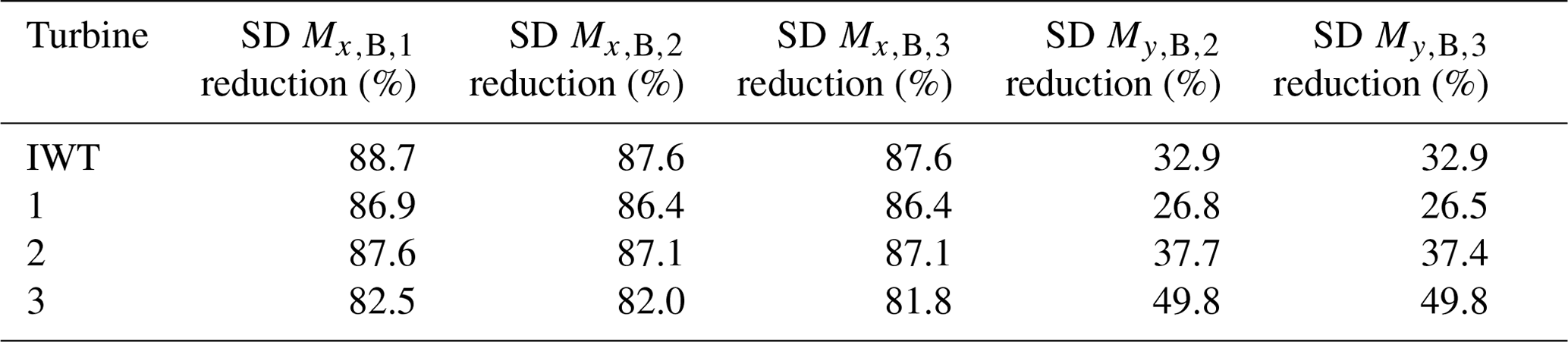
To verify the previous results are valid for other turbine designs, especially commercial ones, exemplary data binning is then repeated for three commercial turbines. All 16 bins for Φ_r,B and $M_{y,\mathrm{B},\mathrm{1}}$ are applied. Table 7 gives the results in relative reduction in standard deviations after the bin counts. The first row contains the IWT7.5-164 results as a reference.

3.4 Verification by finite-element simulations

To relate the results of the data binning to stress amplitude, the following comparisons repeat the simulations with the full-rotor model described in Sect. 3.2. Instead of the time series values for each rotor blade, the values of dependent signals are now varied by the standard deviation. As the extreme stresses in the bolt hole at 90° coincide with the extreme $M_{x,\mathrm{B},\mathrm{1}}$, these evaluations omit steps in between. The difference between the stresses obtained at minimum and maximum $M_{x,\mathrm{B},\mathrm{1}}$ is the stress amplitude of the rotation. The simulations further use the combination of all 16 bins for Φ_r,B and $M_{y,\mathrm{B},\mathrm{1}}$.

Table 8 Variation with standard deviations.

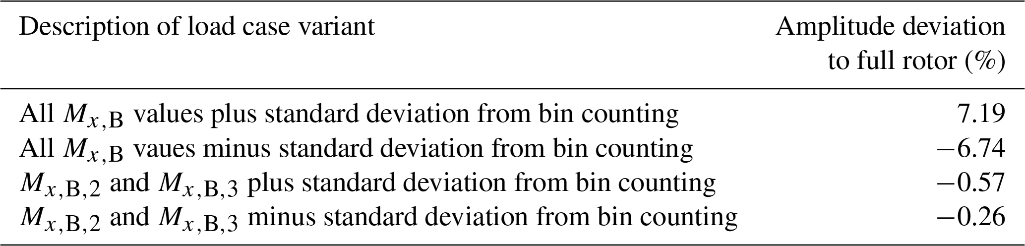
Table 8 lists the influence of variations in all M_x,B signals and only secondary M_x,B signals on this stress amplitude at the 90° position in comparison to a simulation of the full rotor with all loads from the time series. The first two lines show the results of inputs Φ_r,B and $M_{y,\mathrm{B},\mathrm{1}}$ from time series and all other signals from bin counts. The first line changes all M_x,B signals by data binning results plus the standard deviation. These variations in all M_x,B signals lead to significant changes in the stress amplitude. The value deviations are bigger than the deviations between the one-third and full rotor and are thus not acceptable. The load case definition cannot rely only on Φ_r,B and $M_{y,\mathrm{B},\mathrm{1}}$.

Hence, $M_{x,\mathrm{B},\mathrm{1}}$ is introduced as a further independent parameter of the load case definition. Lines three and four show the results of this addition. It leads to far better results in comparison to the 2D load case definition and surpasses the results of the one-third-rotor model as well.

Menck et al. (2020)

Table 9 Preliminary load case selection for pitch bearing ring and hub fatigue simulations.

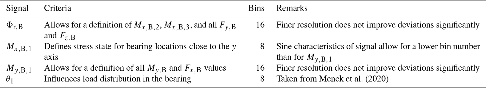
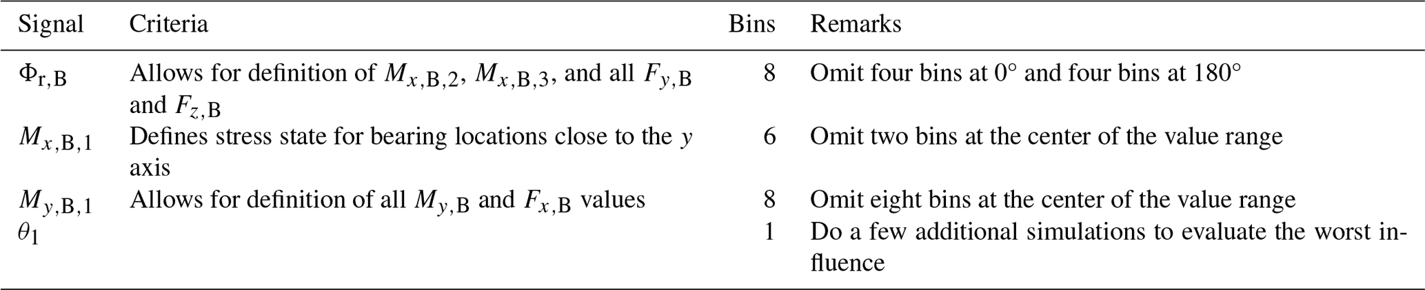
Table 10 Final load case selection for pitch bearing ring fatigue simulations.

3.5 Selection of load cases

Table 9 lists the selected independent signals and the respective bins, resulting in a total of 16 384 load cases. A total of 27 out of the 256 combinations from the stacked data binning involving an azimuth angle and a flapwise bending moment yielded zero samples. These instances occurred exclusively at the edges of the bin ranges. As such, omitting these cases carries no adverse consequences, effectively reducing the overall required load cases to 14 656.

Further on, the selection of eight distinct pitch angles is derived from previous work and has not yet been validated for the purpose of the structural fatigue calculations. Based on just one pitch angle for the simulation, the load cases reduce to 1832. With the computational resources available for this work, this number is still too high for reasonable calculation times. Further reductions for the calculations of pitch bearing ring fatigue are possible if load cases in between extreme values of $M_{x,\mathrm{B},\mathrm{1}}$ and $M_{y,\mathrm{B},\mathrm{1}}$ are omitted and the results are interpolated between the remaining values. This keeps the important simulation load cases that give stress amplitudes. Table 10 lists the resulting number of cases, which result in a total of 384 simulations and are in the range of simulations done in Menck et al. (2020).

4 Discussion and conclusions

The present work covers the selection of load cases for finite-element simulation of wind turbine rotors. Such simulations are used for the design of pitch bearings and hubs. Given the substantial complexity and size of the finite-element models, conducting a large number of simulations within a reasonable time frame becomes challenging. Detailed fatigue calculations, however, necessitate such a large number of simulations to establish the nonlinear relationships between external loads and internal stresses or contact pressures.

To address this challenge, the present study aims to uncover relations in between individual loads of the rotor blade roots and loads and the rotational position of the hub center. This is accomplished through the use of stacked data binning and an evaluation of standard deviations of other signals within the equidistant bins. In addition to the blade root load signals used in approaches documented in the literature, this study incorporates the blade azimuth angle and the rotor out-of-plane moments for the evaluations. Novel methods for deriving these signals from the blade roots' loads are proposed. The algorithm introduced for calculating the blade azimuth angle has undergone successful testing.

The inclusion of the blade's azimuth angle, denoted as Φ_r,B, renders promising outcomes by narrowing down the range of values of the edgewise bending moments. When combined with $M_{y,\mathrm{B},\mathrm{1}}$ and $M_{x,\mathrm{B},\mathrm{1}}$, this integration significantly reduces deviations across all load components in comparison to the original data set and was proven to result in similar stress cycle amplitudes to the simulation of a full rotor with load cases based on time series. The maximum deviation of stress amplitudes in the case study was 0.57 %. To result in a reasonable number of simulations, however, it was necessary to remove bins which result in stress values at the center of the value range. This made the approach more similar to the rain-flow-count-based one in Becker and Jorgensen (2023).

Introducing the out-of-plane rotor moment proves to be beneficial when combined with the blade azimuth angle and flapwise bending moment. However, it is important to note that this addition brings an extra dimension to the parameter space of the simulation load cases, resulting in higher computational costs. Based on the findings of the data binning and exemplary finite-element simulations, the blade azimuth angle and the bending moments of the primary blade bearing are chosen for the load case definition of full-rotor simulations. The present work verified this approach for one exemplary turbine and the use case of pitch bearing ring fatigue.

Future works in this field could explore the use of bins with different lengths and/or mathematical functions to describe the sine-like load components.

Appendix A: Calculation of missing time series signals

Some of the commercial data sets for this work did not have all of the signals described in Sect. 2.2 on input data. Re-creating the data sets was not possible with reasonable methods. Hence, some of the signals were calculated as functions of other signals. This section covers the calculation methods and verifies the calculation of the blade's azimuth angle by the exemplary data set used in the case study.

A1 Calculation approaches

The following calculation approaches were used:

• Pitch angles of secondary blades. Although modern turbines can have individual pitch control and differing pitch angles between the blades, it is permissible to assume the same pitch angles on all three blade roots. In comparison to the larger angle changes performed by the collective pitch to control the turbine's power, the smaller travel distances of the individual pitch have a negligible cross-influence between the individual blade roots.

• Out-of-plane rotor moments. The out-of-plane rotor moments M_y,H and M_z,H in a fixed frame of reference can be calculated from the individual flapwise blade root moments. This assumes Φ_r,B as per Fig. 4.

  $$\begin{array}{}\text{(A1)}& {\displaystyle }\begin{array}{rl}{M}_{y,\mathrm{H}}=& M_{y,\mathrm{B},\mathrm{1}}\cdot \cos \left({\mathrm{\Phi }}_{\mathrm{r},\mathrm{B}}\right)-\cos \left({\mathrm{\Phi }}_{\mathrm{r},\mathrm{B}}+{\displaystyle \frac{\mathrm{2}}{\mathrm{3}}}\mathit{\pi }\right)\\ & \times (M_{y,\mathrm{B},\mathrm{2}}+M_{y,\mathrm{B},\mathrm{3}})\end{array}\text{(A2)}& {\displaystyle }\begin{array}{rl}{M}_{z,\mathrm{H}}=& M_{y,\mathrm{B},\mathrm{1}}\cdot \sin \left({\mathrm{\Phi }}_{\mathrm{r},\mathrm{B}}\right)-\sin \left({\mathrm{\Phi }}_{\mathrm{r},\mathrm{B}}+{\displaystyle \frac{\mathrm{2}}{\mathrm{3}}}\mathit{\pi }\right)\\ & \times (M_{y,\mathrm{B},\mathrm{2}}+M_{y,\mathrm{B},\mathrm{3}})\end{array}\end{array}$$

• Blade azimuth angle. As the edgewise bending moments of the rotor blades are dominated by gravitational forces, the 1p component of M_x,B links directly to the blade azimuth angle Φ_r,B. An algorithm to obtain Φ_r,B can be outlined as follows for each time series file.

  1. Define the 0° position for Φ_r,B, e.g., at the local maximum of the first derivative of M_x,B.

  2. Apply a low-pass filter to M_x,B to eliminate high-frequency components.

  3. If necessary, calculate the derivative of M_x,B.

  4. Identify local maxima or minima.

  5. Check for consistency; i.e., remove extreme values in unrealistic proximity to each other from the analysis.

  6. For each space between extreme values, calculate the linearly increasing vector ranging from 0 to 360° or 0 to 2π for the time steps from one extreme value to the next.

  7. Paste the resulting vector at the corresponding positions into a new ${\mathrm{\Phi }}_{\mathrm{r},\mathrm{B},\text{calc}}$ signal in the file.

  8. For a leading or trailing incomplete rotation of the rotor, use portions of the adjacent full vector.

  This algorithm reproduces speed changes between full-rotor revolutions but not within a revolution. It is essentially equivalent to taking the inverse sine of the 1p component of the edgewise bending moment observed at one of the blade roots.

A2 Blade azimuth angle verification

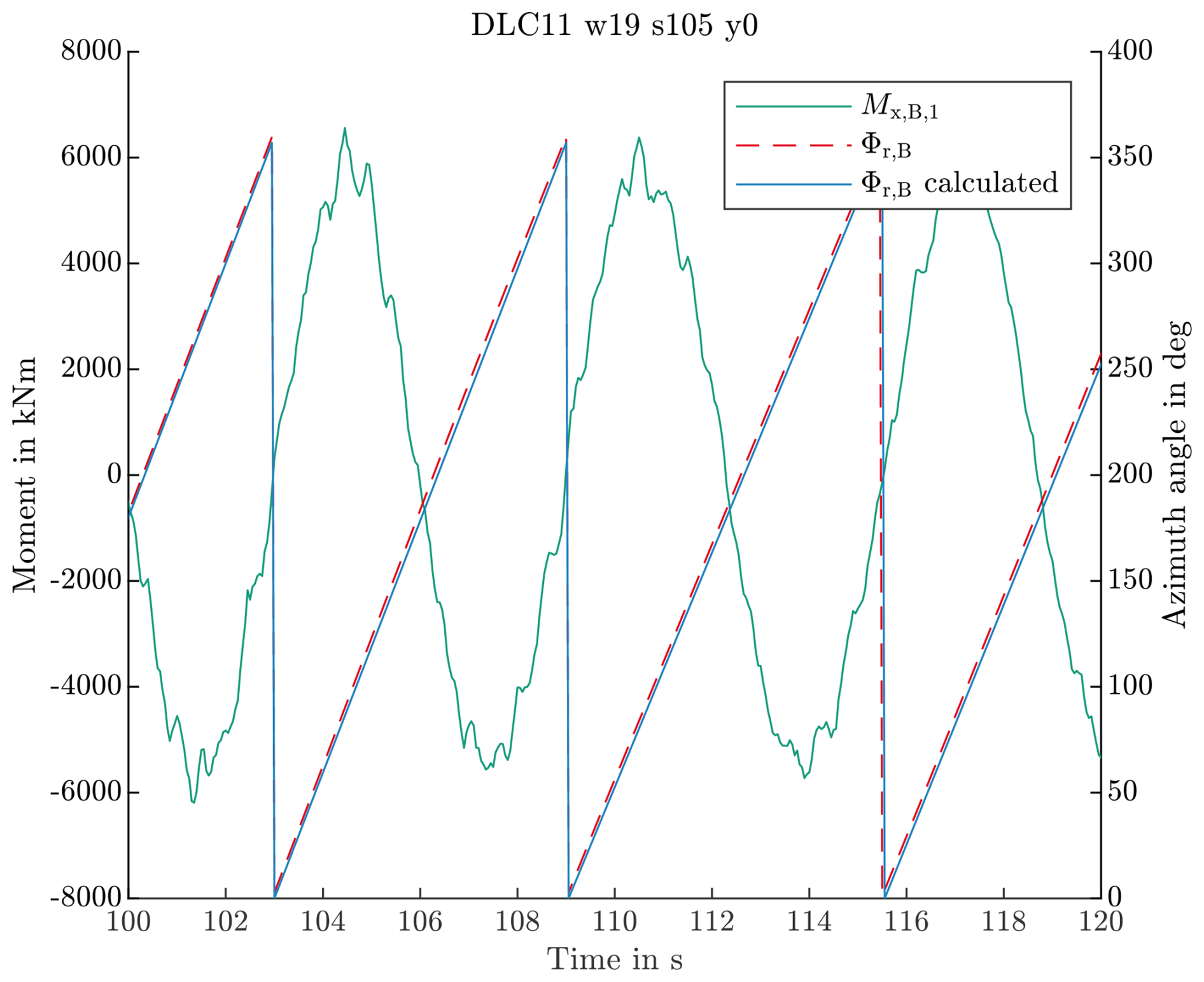
To verify the Φ_r,B calculation, Φ_r,B was calculated for the entire data set of the IWT7.5-164 reference turbine. This data set contains the original signal, so it can be compared against the calculated signal. Figure A1 visualizes exemplary results. The original values are shown as a dashed red line and the calculated values as a blue line. To provide a reference, the figure also includes $M_{x,\mathrm{B},\mathrm{1}}$. The zero position for the calculated azimuth angle was aligned to the local maxima of the derivative of the filtered $M_{x,\mathrm{B},\mathrm{1}}$. A slight phase shift is observable, attributed to the fact that $M_{x,\mathrm{B},\mathrm{1}}$ is not precisely zero at the upper dead point of the blade's circular motion. This load case at a mean wind speed of 19 m s⁻¹ showed a comparatively pronounced frequency content above 1p in $M_{x,\mathrm{B},\mathrm{1}}$ and is displayed to show the robustness of the algorithm.

Figure A1 Exemplary comparison of original and calculated Φ_r,B.

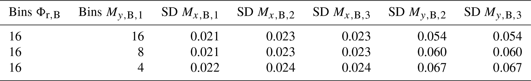
To assess the validity of the calculated azimuth angle signal ${\mathrm{\Phi }}_{\mathrm{r},\mathrm{B},\text{calc}}$ for data binning, Table A1 reproduces some of the bin combinations of Table 6 with the calculated azimuth angle. The results in Table A1 exhibit only very minor differences when compared to those in Table 6.

Table A1 Combined bin count results with varying bins for ${\mathrm{\Phi }}_{\mathrm{r},\mathrm{B},\text{calc}}$ and $M_{y,\mathrm{B},\mathrm{1}}$.