Coleman-free aero-elastic stability methods for three- and two-bladed floating wind turbines

An accurate prediction of aerodynamic damping is important for floating wind turbines, which can enter into resonant low-frequency motion. The Coleman transform is not directly valid for the stability analysis of two-bladed floating wind turbines without applying an additional method to eliminate the system matrix time dependence. Therefore, here we pursue methods that do not rely on it. We derive a time domain model that takes into account the dynamic stall phenomenon and is used for developing Coleman-free aero-elastic stability analysis methods which can quantify the damping without actual simulation. It contains four structural degrees of freedom, namely the floater's pitch angle and the three blade deflection amplitudes, as well as three dynamic stall aerodynamic degrees of freedom, one for each blade. The time domain model is linearized by considering part of the aerodynamic forcing as an added damping contribution. The linearized model is then made time-independent through the application of Hill's or Floquet's method. This enables the possibility of carrying out a stability analysis where the eigenvalue results obtained with both methods are compared. A first modal analysis serves to demonstrate the influence of aerodynamic damping through the variation of the dynamic stall time constant. Thereafter, a second modal analysis is reported as a Campbell diagram also for cross-comparison of the Hill- and Floquet-based results. Moreover, the blade degrees of freedom are converted from the rotational basis to the non-rotational one using the Coleman transform so that results in both frames can be further cross-validated. Finally, we apply the validated stability methods to a two-bladed floating wind turbine and demonstrate their functionality. The stability analysis for the two-bladed wind turbine yields new insight into the blade modal damping and is discussed with comparison to the three-bladed analysis.

1 Introduction

Expanding offshore wind power beyond the usual water depth limit of 50 to 70 m will unlock up to 10 times more energy potential, positioning it as a worldwide source of clean energy (Stiesdal Offshore, 2023). Floating wind turbines have been developed since the Hywind demonstrator from 2009 with the intent to extract energy in deeper waters, and they are estimated to be capable of being installed at depths reaching up to 1000 m (CORROSION, 2023). This endeavour pushes the development of floating wind turbines for the ScotWind and INTOG (Innovation and Targeted Oil and Gas) projects in Scotland to deliver by 2035 a cumulative capacity of 24.7 GW in floating wind energy (Offshore Wind Scotland, 2024). The design of floating wind turbines relies heavily on aero-elastic modelling of the system response. For a dynamic model described in the time domain, the rotation of the rotor introduces multiple time periodic terms in the governing equations that are based on physical effects. Due to the system's periodicity, a standard eigenvalue analysis through a constant system matrix is not possible. The aero-elastic stability analysis is an important calculation for the design of wind turbines that addresses the damping of the structural modes as well as the aerodynamic damping contribution. This damping is of high importance for the low-frequency pitch motion of floating wind turbines. Usually the aero-elastic stability analysis is carried out with a linearized version of the turbine dynamic model by applying a Coleman transform (Coleman et al., 1957) which eliminates the system's periodicity. This elimination, also referred to as the Coleman or the multi-blade coordinate (MBC) transform, is only applicable for a rotor containing three blades or more and for isotropic systems. Theoretically, the conditions to be fulfilled for a rotor to be viewed as isotropic are not to be subjected to gravity effects or a skewed or sheared inflow and to not have a tilt angle either. For floating wind turbines, the aero-elastic stability analysis is further complicated due to the presence of the floater’s degrees of freedom which introduce low-frequency modes. For this reason, there is a need to establish aero-elastic stability methods that are valid for floating two-bladed wind turbines and that do not rely on the Coleman transform.

Certain past investigations on methods that render a system linear time-invariant (LTI) have been proven to be less efficient and more computationally expensive to put into practice compared to other more novel methods or even the Coleman approach. For example, it was proposed by Bir (2008) to use an averaged system matrix over a period as an alternative to computing the system matrix at certain sampled times steps, but that method does not accurately take into consideration the full periodicity of the system. As a remedy to this problem for the treatment of the system's periodicity, the Hill (1886) determinant method was employed by Hansen (2016) for the modal analyses of an onshore two-bladed and three-bladed wind turbine. Alternatively, the Coleman transform is applied both in the aero-hydro-servo-elastic OpenFAST code (Bortolotti et al., 2024) and in the aero-servo-elastic HAWCStab2 code (Hansen, 2004; Kim et al., 2013; Madsen et al., 2020). As another alternative, in their respective studies, Bottasso and Cacciola (2015) and Riva (2017) employed the Floquet (1883) theory to completely eliminate the periodicity so that the stability of a simplified onshore three-bladed wind turbine could be assessed (Skjoldan, 2011). Similarly and more recently, Meng et al. (2024) researched the impact of aerodynamic states on the stability analysis by applying the Coleman transform to directly eliminate the periodicity of a floating wind turbine, followed by a modal order reduction. With a similar main scope in mind, in our past work the linearization of a floating wind turbine's simplified equations of motion was already realized (Pamfil et al., 2024) by relying on Hill's method but without taking into account all kinematic effects that influence the blade motion or having implemented yet a dynamic stall model.

The purpose of the present study is to compare and validate Hill's and Floquet's methods for the stability analysis of a floating wind turbine. In this context, we aim to clarify four objectives stated as questions: (1) how the effect of the floater tilt is involved in the stability analysis, (2) if the damping effects of the aerodynamic states can be consistently included, (3) if the results of the two methods agree and can reproduce the forward- and backward-whirling rotor modes in a Coleman-based analysis, and (4) if the methods can successfully be applied to a two-bladed floating wind turbine. Hence, to answer these questions, we derive a simplified floating wind turbine model which has four structural degrees of freedom (DOFs), being the three blade deflection amplitudes and a platform pitch angle. This time domain model is then enhanced by including Øye's linearized dynamic stall model (Øye, 1991) through the consideration of one extra dynamic stall aerodynamic degree of freedom per blade. The dynamic stall simulations are used as a benchmark for comparison between the time domain model and a linear model which is obtained by a full linearization of the aerodynamic damping load. After it is assessed if the linear model is assembled correctly and if it is physically consistent, we render it linear time-invariant (LTI) by applying Hill's or Floquet's method in order to be exempt from having to apply the Coleman transform. By relying on either method, we conduct a first set of stability analyses for a varying dynamic stall model time constant and a second set of studies for a variation of the rotational speed, and these are displayed as Campbell diagrams. Regarding the applicability of Hill's and Floquet's methods on the system matrix, the resulting eigenvalues are compared with the ones found through the Coleman transform by reconstructing the rotor forward-whirling (FW) and backward-whirling (BW) modes. The results of these analyses are further verified through a cross-validation of the eigenvalues for a two-bladed floating wind turbine model.

We achieve the first objective about finding the impact of the floater tilt on the stability analysis by showing that the structural equations of motion (EOMs) do not depend on the equilibrium floater tilt position when neglecting gravity effects and assuming a small tilt angle. This implies that for our model the equilibrium floater tilt position does not affect the stability analysis. Secondly, aerodynamic states are included in the linear model's state-space system, and they do affect the modal damping and damped frequencies as showcased through the stability analysis results. The third objective is fulfilled by proving first that either Hill's or Floquet's stability method is able to capture the correct principal damped frequencies in the original frame, which is called the rotational frame. It is also proved that these eigenvalues can be expressed in a modified frame called the non-rotational frame to match the ones found through the Coleman-transformed system matrix. On that matter, the LTI model derived with Hill's method fully takes into consideration the periodicity of the system, making it possible to calculate the principal damped frequencies and the periodically shifted frequencies. The fourth and last objective is fulfilled by developing the two-bladed wind turbine model and revealing that the same methods as for a three-bladed rotor can be applied to obtain correct stability results. We also observe a marked difference in blade modal damping behaviour for the two-bladed floating wind turbine compared to the three-bladed case.

2 Floating wind turbine model description

The floating wind turbine model that is being studied has four structural degrees of freedom (DOFs) as schematized in Fig. 1. For a three-bladed wind turbine, the four structural DOFs are the blade flap-wise deflection amplitudes, labelled as a_l with a blade identification index of $l=\mathrm{1},\mathrm{2},\mathrm{3}$, and the floater pitch angular motion, labelled as ξ₅. These four structural DOFs are represented in a vector form as $\mathit{x}={\left[{\mathit{\xi }}_{\mathrm{5}},a_{\mathrm{1}},a_{\mathrm{2}},a_{\mathrm{3}}\right]}^{\mathrm{T}}$. Three additional aerodynamic DOFs are included later to account for the dynamic stall phenomenon. The floating wind turbine blade structural properties, such as its blade mode shapes ϕ, natural frequencies ω, and the blade mass per unit length m(r), are taken from the DTU 10 MW reference wind turbine (Bak et al., 2013). In Fig. 1, d identifies a reference radial position from the hub along the blade of length L_b with d=0.7L_b, i.e. at 70 % of the blade length span. For simplicity, the aerodynamic force for each blade F_l,aero is calculated at that reference distance r=d from the blade root, which is representative of the full blade in terms of applied aerodynamic loads. The floating wind turbine is subjected to an inflow velocity V₀ at hub height H, to a forcing moment M_F applied at the floater base, and to a constant rotor rotational speed of Ω. Here, $K_{{\mathit{\xi }}_{\mathrm{5}}}$ refers to the rotational stiffness coefficient along the floater pitch angle ξ₅, and M is the cumulative mass of the hub and nacelle combined.

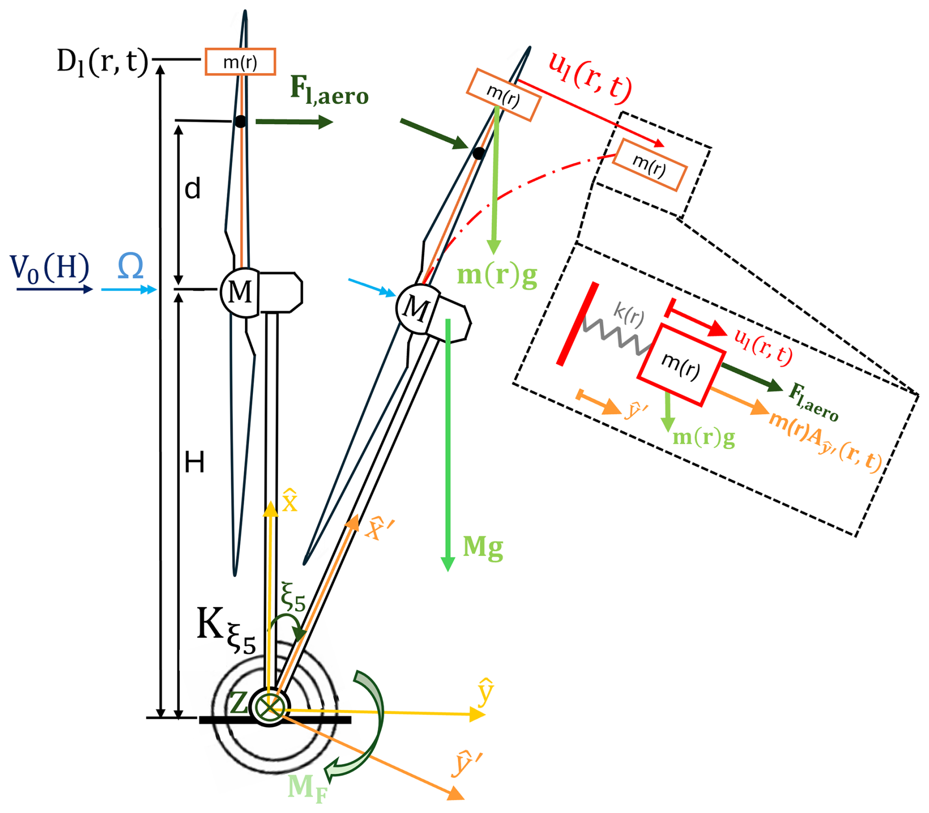
Figure 1 Schematic representation of the four structural DOFs of the floating wind turbine model where m(r) is the blade's mass distribution at the radial location r, u_l(r,t) is the blade deflection, and the index l refers to the blade identification.

The blade deflection u_l(r,t) is approximated through the consideration of the first flap mode (1f) only, which is characterized by a mode shape ϕ_1f and a natural frequency ω_1f, resulting in $u_l(r,t)={\mathit{\varphi }}_{\mathrm{1}\mathrm{f}}\left(r\right)a_l\left(t\right)$.

Furthermore, the time-dependent (t) azimuthal angular position Ψ_l of the blades is defined in radians as

$$\begin{array}{}\text{(1)}& {\mathrm{\Psi }}_l\left(t\right)={\displaystyle \frac{\mathrm{2}\mathit{\pi }}{N_{\mathrm{b}}}}\left(l-\mathrm{1}\right)+\mathrm{\Omega }t,\end{array}$$

where N_b is the rotor's number of blades, and the rotational speed Ω is connected to a corresponding period T through the ratio of $T=\mathrm{2}\mathit{\pi }/\mathrm{\Omega }$.

In Fig. 1, a global fixed coordinate system is defined in terms of unit vectors $\widehat{\mathit{x}}$ and $\widehat{\mathit{y}}$. Additionally, there is a local moving coordinate system that rotates with the blade and describes the position of a blade section of mass m(r). That coordinate system defines the radial location of mass m(r) with the unit vector ${\widehat{\mathit{x}}}^{\prime }\left(t\right)$ and its tangential motion as the blade is deflected in the direction of unit vector ${\widehat{\mathit{y}}}^{\prime }\left(t\right)$. Based on the perpendicularity of these unit vectors, an out-of-plane vector $\widehat{\mathit{z}}$ is the result of a cross product between them, such that $\widehat{\mathit{z}}={\widehat{\mathit{x}}}^{\prime }\times {\widehat{\mathit{y}}}^{\prime }$ and $-\widehat{\mathit{z}}={\widehat{\mathit{y}}}^{\prime }\times {\widehat{\mathit{x}}}^{\prime }$. The radial position in the ${\widehat{\mathit{x}}}^{\prime }\left(t\right)$–${\widehat{\mathit{y}}}^{\prime }\left(t\right)$ coordinate system of a blade's element mass m(r) is $D_l(r,t)=H+r\cos {\mathrm{\Psi }}_l\left(t\right)$, and its tangential displacement is the blade deflection u_l(r,t). The vector representation of the mass m(r)'s displacement, ${\widehat{\mathit{D}}}_l(r,t)$, in the moving rotating coordinate system ${\widehat{\mathit{x}}}^{\prime }\left(t\right)$–${\widehat{\mathit{y}}}^{\prime }\left(t\right)$ is thus

$$\begin{array}{}\text{(2)}& {\widehat{\mathit{D}}}_l(r,t)=D_l(r,t){\widehat{\mathit{x}}}^{\prime }\left(t\right)+u_l(r,t){\widehat{\mathit{y}}}^{\prime }\left(t\right).\end{array}$$

As mentioned earlier, the blade deflection u_l(r,t) is quantified by the product of the first flap mode shape ϕ_1f(r) in the direction tangential to the rotor plane with the blade displacement amplitude a_l(t).

2.1 Equations of motion

A time domain model is developed with the initial purpose of obtaining the steady-state responses for a given operational point. It also serves as a foundation to afterwards linearize the aerodynamically damped forcing as a damping matrix contribution and to include the dynamic stall DOF equations in the system matrices. As a starting point, it is observable in Fig. 1 that the unit vectors ${\widehat{\mathit{x}}}^{\prime }$ and ${\widehat{\mathit{y}}}^{\prime }$ can be represented using the global fixed coordinates $\widehat{\mathit{x}}$ and $\widehat{\mathit{y}}$ after applying a rotation transformation, respectively as ${\widehat{\mathit{x}}}^{\prime }=\cos \left({\mathit{\xi }}_{\mathrm{5}}\right)\widehat{\mathit{x}}+\sin \left({\mathit{\xi }}_{\mathrm{5}}\right)\widehat{\mathit{y}}$ and ${\widehat{\mathit{y}}}^{\prime }=-\sin \left({\mathit{\xi }}_{\mathrm{5}}\right)\widehat{\mathit{x}}+\cos \left({\mathit{\xi }}_{\mathrm{5}}\right)\widehat{\mathit{y}}$. They are then derived in time to obtain ${\dot{\widehat{\mathit{x}}}}^{\prime }={\dot{\mathit{\xi }}}_{\mathrm{5}}{\widehat{\mathit{y}}}^{\prime }$ and ${\dot{\widehat{\mathit{y}}}}^{\prime }=-{\dot{\mathit{\xi }}}_{\mathrm{5}}{\widehat{\mathit{x}}}^{\prime }$. These expressions come in handy when deriving (for the element mass m(r)) its velocity vector ${\widehat{\mathit{V}}}_l(r,t)=\mathrm{d}\left({\widehat{\mathit{D}}}_l(r,t)\right)/\mathrm{d}t$,

$$\begin{array}{}\text{(3)}& \begin{array}{rl}{\widehat{\mathit{V}}}_l(r,t)& ={\dot{D}}_l\left(t\right){\widehat{\mathit{x}}}^{\prime }+D_l(r,t){\dot{\widehat{\mathit{x}}}}^{\prime }\left(t\right)+{\dot{u}}_l(r,t){\widehat{\mathit{y}}}^{\prime }\left(t\right)\\ & +u_l(r,t){\dot{\widehat{\mathit{y}}}}^{\prime }\left(t\right)=\left({\dot{D}}_l(r,t)-u_l(r,t){\dot{\mathit{\xi }}}_{\mathrm{5}}\right){\widehat{\mathit{x}}}^{\prime }\\ & +\left(D_l(r,t){\dot{\mathit{\xi }}}_{\mathrm{5}}+{\dot{u}}_l(r,t)\right){\widehat{\mathit{y}}}^{\prime },\end{array}\end{array}$$

and its acceleration vector ${\widehat{\mathit{A}}}_l(r,t)=\mathrm{d}\left({\widehat{\mathit{V}}}_l(r,t)\right)/\mathrm{d}t$,

$$\begin{array}{}\text{(4)}& \begin{array}{rl}{\widehat{\mathit{A}}}_l(r,t)& =\left({\ddot{D}}_l(r,t)-u_l(r,t){\ddot{\mathit{\xi }}}_{\mathrm{5}}-\mathrm{2}{\dot{u}}_l(r,t){\dot{\mathit{\xi }}}_{\mathrm{5}}-D_l(r,t){\dot{\mathit{\xi }}}_{\mathrm{5}}^{\mathrm{2}}\right){\widehat{\mathit{x}}}^{\prime }\\ & +\left(\mathrm{2}{\dot{D}}_l(r,t){\dot{\mathit{\xi }}}_{\mathrm{5}}+D_l(r,t){\ddot{\mathit{\xi }}}_{\mathrm{5}}+{\ddot{u}}_l(r,t)-u_l(r,t){\dot{\mathit{\xi }}}_{\mathrm{5}}^{\mathrm{2}}\right){\widehat{\mathit{y}}}^{\prime }.\end{array}\end{array}$$

The acceleration vector ${\widehat{\mathit{A}}}_l(r,t)$ can then be linearized by disregarding higher-order terms, which results in

$$\begin{array}{}\text{(5)}& \begin{array}{rl}{\widehat{\mathit{A}}}_l(r,t)& \approx {\widehat{\mathit{A}}}_{l,\mathrm{lin}}(r,t)=\underset{A_{{\widehat{x}}^{\prime },l}}{\underbrace{{\ddot{D}}_l(r,t)}}{\widehat{\mathit{x}}}^{\prime }\\ & +\underset{A_{{\widehat{y}}^{\prime },l}}{\underbrace{\left(\mathrm{2}{\dot{D}}_l(r,t){\dot{\mathit{\xi }}}_{\mathrm{5}}+D_l(r,t){\ddot{\mathit{\xi }}}_{\mathrm{5}}+{\ddot{u}}_l(r,t)\right)}}{\widehat{\mathit{y}}}^{\prime }.\end{array}\end{array}$$

We observe in Eqs. (3) and (4) that none of the nonlinear terms include ξ₅ as a factor. For this reason, the linearized model is applicable for any steady-state value of ξ₅. Finally, we identify in Eq. (5) the tangential acceleration $A_{{\widehat{y}}^{\prime },l}$ that is relevant to describe the element mass m(r)'s inertial force $f_{{\widehat{y}}^{\prime },l}(r,t)=m\left(r\right)A_{{\widehat{y}}^{\prime },l}(r,t)$. To build up the EOM for the linearized total moment applied around the $\widehat{\mathit{z}}$ axis, the angular momentum theory is used to compute the inertia moment p_l(r,t) which translates to

$$\begin{array}{}\text{(6)}& p_l(r,t)={\displaystyle \frac{\mathrm{d}}{\mathrm{d}t}}\left({\widehat{\mathit{D}}}_l(r,t)\times \left(m\left(r\right){\widehat{\mathit{V}}}_l(r,t)\right)\right).\end{array}$$

The inertia moment p_l(r,t) is then approximated as $p_{l,\mathrm{lin}}(r,t)$ by neglecting higher-order terms, which gives

$$\begin{array}{}\text{(7)}& \begin{array}{rl}{p}_l(r,t)& \approx p_{l,\mathrm{lin}}(r,t)=m\left(r\right)\left(D_l^{\mathrm{2}}(r,t)\ddot{{\mathit{\xi }}_{\mathrm{5}}}\right.\\ & +\mathrm{2}{D}_l(r,t){\dot{D}}_l(r,t)\dot{{\mathit{\xi }}_{\mathrm{5}}}+D_l(r,t){\ddot{u}}_l(r,t)\\ & \left.-{\ddot{D}}_l(r,t)u_l(r,t)\right).\end{array}\end{array}$$

These kinematic formulas can be used to establish the equations of rotational motion around the $\widehat{\mathit{z}}$ axis and of translational motion along the ${\widehat{\mathit{y}}}^{\prime }$ axis which corresponds to the tangential direction of the blade rotation around the floater base. The inertia contribution of the hub and nacelle cumulative mass M is translated from the hub height to the floater's base point with a distance H that separates the two points, MH². The remaining share of the rotational inertia around the $\widehat{\mathit{z}}$ axis is due to the blade's distributed mass m(r)'s effect on the inertial moment $p_{l,\mathrm{lin}}(r,t)$. The rotational motion equation for moments around the $\widehat{\mathit{z}}$ axis is written as

$$\begin{array}{}\text{(8)}& \begin{array}{rl}\widehat{\mathit{z}}& :M{H}^{\mathrm{2}}{\ddot{\mathit{\xi }}}_{\mathrm{5}}\mathit{\delta }{\mathit{\xi }}_{\mathrm{5}}+\sum _{l=\mathrm{1}}^{N_{\mathrm{b}}}\left(\underset{\mathrm{0}}{\overset{L_{\mathrm{b}}}{\int }}{p}_{l,\mathrm{lin}}(r,t)\mathrm{d}r\mathit{\delta }{\mathit{\xi }}_{\mathrm{5}}\right)\\ & +K_{{\mathit{\xi }}_{\mathrm{5}}}{\mathit{\xi }}_{\mathrm{5}}\mathit{\delta }{\mathit{\xi }}_{\mathrm{5}}=M_{\mathrm{F}}\mathit{\delta }{\mathit{\xi }}_{\mathrm{5}}+\underset{M_{\mathrm{aero}}}{\underbrace{\left(\sum _{l=\mathrm{1}}^{N_{\mathrm{b}}}{D}_l(d,t)F_{l,\mathrm{aero}}\left(t\right)\right)}}\mathit{\delta }{\mathit{\xi }}_{\mathrm{5}},\end{array}\end{array}$$

after using the principle of virtual work with a δξ₅ rotation. The applied forces on the right-hand side of Eq. (8) include M_F, which is the moment applied directly on the floater DOF ξ₅, and an aerodynamic moment M_aero contribution through F_l,aero. As seen in Fig. 1, the aerodynamic moment M_aero is induced by an equivalent total aerodynamic forcing F_l,aero applied on each blade with a moment arm $D_l(d,t)=H+d\cos {\mathrm{\Psi }}_l\left(t\right)$ at the reference location of r=d. This aerodynamic forcing is an approximation of the total contribution by a local load F_l integrated over the entire blade length span as $F_{l,\mathrm{aero}}=F_l{L}_{\mathrm{b}}$.

Similarly, the equation of translational motion along the ${\widehat{\mathit{y}}}^{\prime }$ axis for each lth blade is found based on the principle of the blade displacement virtual work $\mathit{\delta }{u}_l(r,t)=\mathit{\delta }{a}_l\left(t\right){\mathit{\varphi }}_{\mathrm{1}\mathrm{f}}\left(r\right)$:

$$\begin{array}{}\text{(9)}& \begin{array}{rl}{\widehat{\mathit{y}}}^{\prime }& :\underset{\mathrm{0}}{\overset{L_{\mathrm{b}}}{\int }}\underset{f_{{\widehat{y}}^{\prime },l}(r,t)}{\underbrace{m\left(r\right)A_{{\widehat{y}}^{\prime },l}(r,t)}}\mathit{\delta }{a}_l{\mathit{\varphi }}_{\mathrm{1}\mathrm{f}}\left(r\right)\mathrm{d}r\\ & +\underset{K_{a_l}{a}_l\mathit{\delta }{a}_l}{\underbrace{\underset{\mathrm{0}}{\overset{L_{\mathrm{b}}}{\int }}k\left(r\right)a_l\left(t\right){\mathit{\varphi }}_{\mathrm{1}\mathrm{f}}\left(r\right)\left(\mathit{\delta }{a}_l{\mathit{\varphi }}_{\mathrm{1}\mathrm{f}}\left(r\right)\right)\mathrm{d}r}}\\ & =\underset{{\mathrm{GF}}_{a_l}}{\underbrace{F_{l,\mathrm{aero}}\left(t\right){\mathit{\varphi }}_{\mathrm{1}\mathrm{f}}\left(d\right)}}\mathit{\delta }{a}_l,\end{array}\end{array}$$

where there is a consideration of the blade aerodynamic forcing F_l,aero and the tangential inertia force $f_{{\widehat{y}}^{\prime }}(r,t)$. In Eq. (9), k(r) is the blade sectional stiffness as $k\left(r\right)=m\left(r\right){\mathit{\omega }}_{\mathrm{1}\mathrm{f}}^{\mathrm{2}}$, and ϕ_1f(d) is the first flap mode's value at the reference radial location r=d. The internal force which is caused by the element mass m(r)'s stiffness coefficient k(r) is not appearing in Eq. (8) because it is not an external force applied to the system. The external force that is considered in Eq. (9) is the generalized aerodynamic blade force GF${}_{a_l}$.

The right-hand side for both the rotational and translational equations of motion is part of the time domain model's forcing vector, denoted F_T. The time (index T) domain model's dynamics are described by the following overall EOM:

$$\begin{array}{}\text{(10)}& {\mathbf{M}}_S\ddot{\mathit{x}}+{\mathbf{C}}_S\dot{\mathit{x}}+{\mathbf{K}}_S\mathit{x}={\mathit{F}}_T,\end{array}$$

where there is only a structural (index S) damping C_S.

The structural mass M_S and stiffness K_S matrices include a contribution due to the floater and overall turbine (nacelle and tower) structural properties (M_S,floater and K_S,floater). The other contribution originates from the blade (M_S,blades(r) and K_S,blades(r)) structural properties through an integration span-wise in direction r. Therefore, for the three-bladed wind turbine, the structural mass ${\mathbf{M}}_S={\mathbf{M}}_{S,\mathrm{floater}}+{\int }_{\mathrm{0}}^{L_{\mathrm{b}}}{\mathbf{M}}_{S,\mathrm{blades}}\left(r\right)\mathrm{d}r$ and stiffness ${\mathbf{K}}_S={\mathbf{K}}_{S,\mathrm{floater}}+{\int }_{\mathrm{0}}^{L_{\mathrm{b}}}{\mathbf{K}}_{S,\mathrm{blades}}\left(r\right)\mathrm{d}r$ matrices are assembled as

$$\begin{array}{}\text{(11)}& \begin{array}{rl}& {\mathbf{M}}_S=\left[\begin{array}{cccc}M{H}^{\mathrm{2}}& \mathrm{0}& \mathrm{0}& \mathrm{0}\\ \mathrm{0}& \mathrm{0}& \mathrm{0}& \mathrm{0}\\ \mathrm{0}& \mathrm{0}& \mathrm{0}& \mathrm{0}\\ \mathrm{0}& \mathrm{0}& \mathrm{0}& \mathrm{0}\end{array}\right]\\ & +\underset{\mathrm{0}}{\overset{L_{\mathrm{b}}}{\int }}m\left(r\right)\left[\begin{array}{cccc}{\sum }_{l=\mathrm{1}}^{\mathrm{3}}{D}_l^{\mathrm{2}}(r,t)& D_{\mathrm{1}}(r,t){\mathit{\varphi }}_{\mathrm{1}\mathrm{f}}\left(r\right)& D_{\mathrm{2}}(r,t){\mathit{\varphi }}_{\mathrm{1}\mathrm{f}}\left(r\right)& D_{\mathrm{3}}(r,t){\mathit{\varphi }}_{\mathrm{1}\mathrm{f}}\left(r\right)\\ D_{\mathrm{1}}(r,t){\mathit{\varphi }}_{\mathrm{1}\mathrm{f}}\left(r\right)& {\left({\mathit{\varphi }}_{\mathrm{1}\mathrm{f}}\left(r\right)\right)}^{\mathrm{2}}& \mathrm{0}& \mathrm{0}\\ D_{\mathrm{2}}(r,t){\mathit{\varphi }}_{\mathrm{1}\mathrm{f}}\left(r\right)& \mathrm{0}& {\left({\mathit{\varphi }}_{\mathrm{1}\mathrm{f}}\left(r\right)\right)}^{\mathrm{2}}& \mathrm{0}\\ D_{\mathrm{3}}(r,t){\mathit{\varphi }}_{\mathrm{1}\mathrm{f}}\left(r\right)& \mathrm{0}& \mathrm{0}& {\left({\mathit{\varphi }}_{\mathrm{1}\mathrm{f}}\left(r\right)\right)}^{\mathrm{2}}\end{array}\right]\mathrm{d}r\end{array}\end{array}$$

and

$$\begin{array}{}\text{(12)}& \begin{array}{rl}& {\mathbf{K}}_S=\left[\begin{array}{cccc}{K}_{{\mathit{\xi }}_{\mathrm{5}}}& \mathrm{0}& \mathrm{0}& \mathrm{0}\\ \mathrm{0}& \mathrm{0}& \mathrm{0}& \mathrm{0}\\ \mathrm{0}& \mathrm{0}& \mathrm{0}& \mathrm{0}\\ \mathrm{0}& \mathrm{0}& \mathrm{0}& \mathrm{0}\end{array}\right]\\ & +\underset{\mathrm{0}}{\overset{L_{\mathrm{b}}}{\int }}m\left(r\right)\left[\begin{array}{cccc}\mathrm{0}& -{\ddot{D}}_{\mathrm{1}}(r,t){\mathit{\varphi }}_{\mathrm{1}\mathrm{f}}\left(r\right)& -{\ddot{D}}_{\mathrm{2}}(r,t){\mathit{\varphi }}_{\mathrm{1}\mathrm{f}}\left(r\right)& -{\ddot{D}}_{\mathrm{3}}(r,t){\mathit{\varphi }}_{\mathrm{1}\mathrm{f}}\left(r\right)\\ \mathrm{0}& {\mathit{\omega }}_{\mathrm{1}\mathrm{f}}^{\mathrm{2}}{\left({\mathit{\varphi }}_{\mathrm{1}\mathrm{f}}\left(r\right)\right)}^{\mathrm{2}}& \mathrm{0}& \mathrm{0}\\ \mathrm{0}& \mathrm{0}& {\mathit{\omega }}_{\mathrm{1}\mathrm{f}}^{\mathrm{2}}{\left({\mathit{\varphi }}_{\mathrm{1}\mathrm{f}}\left(r\right)\right)}^{\mathrm{2}}& \mathrm{0}\\ \mathrm{0}& \mathrm{0}& \mathrm{0}& {\mathit{\omega }}_{\mathrm{1}\mathrm{f}}^{\mathrm{2}}{\left({\mathit{\varphi }}_{\mathrm{1}\mathrm{f}}\left(r\right)\right)}^{\mathrm{2}}\end{array}\right]\mathrm{d}r,\end{array}\end{array}$$

in accordance with the rotational and translational equations of motion in Eqs. (8) and (9). As observable in Eq. (12), the inertia moment $p_{l,\mathrm{lin}}(r,t)$ generates negative restoring forces that are equivalent to a negative stiffness effect. Moreover, the restoring floater pitching moment coefficient $K_{{\mathit{\xi }}_{\mathrm{5}}}$ is tuned to achieve a realistic platform pitch frequency of ${\mathit{\omega }}_{{\mathit{\xi }}_{\mathrm{5}}}=\mathrm{0.035}$ Hz.

The structural damping C_S is inspired by a classical Rayleigh damping model, ${\mathbf{C}}_S=\mathit{\nu }{\mathbf{M}}_S+\mathit{\mu }{\mathbf{K}}_S$, where only the diagonal elements of the structural stiffness matrix K_S are multiplying a specific factor μ_k. The off-diagonal components of the structural stiffness matrix K_S are not related to the structural stiffness of the structure itself but rather to the element mass m(r)'s inertial effects which is why they are not considered in the structural damping. Furthermore, including the mass matrix M_S proportionality to the structural damping matrix could potentially over-damp the system at low natural frequencies because the damping ratio contribution due to inertia is inversely proportional to the frequency. In line with Eqs. (8) and (9), the total structural damping ${\mathbf{C}}_S={\mathbf{C}}_{S,\mathrm{floater}}+{\int }_{\mathrm{0}}^{L_{\mathrm{b}}}{\mathbf{C}}_{S,\mathrm{blades}}\left(r\right)\mathrm{d}r$ matrix for the three-bladed wind turbine considers additional effects that are caused by the element mass m(r)'s inertia as revealed below:

$$\begin{array}{}\text{(13)}& \begin{array}{rl}& {\mathbf{C}}_S=\underset{\mathrm{0}}{\overset{L_{\mathrm{b}}}{\int }}m\left(r\right)\\ & \times \left[\begin{array}{cccc}{\sum }_{l=\mathrm{1}}^{\mathrm{3}}\mathrm{2}{D}_l(r,t){\dot{D}}_l(r,t)& \mathrm{0}& \mathrm{0}& \mathrm{0}\\ \mathrm{2}{\dot{D}}_{\mathrm{1}}(r,t){\mathit{\varphi }}_{\mathrm{1}\mathrm{f}}\left(r\right)& {\mathit{\mu }}_{a_{\mathrm{1}}}{\mathit{\omega }}_{\mathrm{1}\mathrm{f}}^{\mathrm{2}}{\left({\mathit{\varphi }}_{\mathrm{1}\mathrm{f}}\left(r\right)\right)}^{\mathrm{2}}& \mathrm{0}& \mathrm{0}\\ \mathrm{2}{\dot{D}}_{\mathrm{2}}(r,t){\mathit{\varphi }}_{\mathrm{1}\mathrm{f}}\left(r\right)& \mathrm{0}& {\mathit{\mu }}_{a_{\mathrm{2}}}{\mathit{\omega }}_{\mathrm{1}\mathrm{f}}^{\mathrm{2}}{\left({\mathit{\varphi }}_{\mathrm{1}\mathrm{f}}\left(r\right)\right)}^{\mathrm{2}}& \mathrm{0}\\ \mathrm{2}{\dot{D}}_{\mathrm{3}}(r,t){\mathit{\varphi }}_{\mathrm{1}\mathrm{f}}\left(r\right)& \mathrm{0}& \mathrm{0}& {\mathit{\mu }}_{a_{\mathrm{3}}}{\mathit{\omega }}_{\mathrm{1}\mathrm{f}}^{\mathrm{2}}{\left({\mathit{\varphi }}_{\mathrm{1}\mathrm{f}}\left(r\right)\right)}^{\mathrm{2}}\end{array}\right]\mathrm{d}r\\ & +\left[\begin{array}{cccc}{\mathit{\mu }}_{{\mathit{\xi }}_{\mathrm{5}}}{K}_{{\mathit{\xi }}_{\mathrm{5}}}& \mathrm{0}& \mathrm{0}& \mathrm{0}\\ \mathrm{0}& \mathrm{0}& \mathrm{0}& \mathrm{0}\\ \mathrm{0}& \mathrm{0}& \mathrm{0}& \mathrm{0}\\ \mathrm{0}& \mathrm{0}& \mathrm{0}& \mathrm{0}\end{array}\right].\end{array}\end{array}$$

To compute each kth DOF's diagonal component in the structural damping matrix C_S, we set the log-decrement δ_k value and then use the structural frequency ω_k to obtain the damping factor μ_k through

$$\begin{array}{}\text{(14)}& {\mathit{\zeta }}_k={\displaystyle \frac{{\mathit{\delta }}_k}{\sqrt{\mathrm{4}{\mathit{\pi }}^{\mathrm{2}}+{\mathit{\delta }}_k^{\mathrm{2}}}}}\approx {\displaystyle \frac{{\mathit{\delta }}_k}{\mathrm{2}\mathit{\pi }}}\text{and}{\mathit{\mu }}_k={\displaystyle \frac{\mathrm{2}{\mathit{\zeta }}_k}{{\mathit{\omega }}_k}}.\end{array}$$

The approximation for ζ_k holds for a considerably small damping ratio ζ_k. The torsional structural damping applied on ξ₅ must represent the hydrodynamic damping effect of the floater's motion. The damping ratio for a TetraSpar floater is found in Borg et al. (2024) as ${\mathit{\zeta }}_{{\mathit{\xi }}_{\mathrm{5}}}=\mathrm{3}$ % with a log-decrement of ${\mathit{\delta }}_{{\mathit{\xi }}_{\mathrm{5}}}=\mathrm{0.20}$. This results in a damping factor of ${\mathit{\mu }}_{{\mathit{\xi }}_{\mathrm{5}}}=\mathrm{0.30}$. Besides, for the blade DOF a_l the damping ratio is set at a very low value of ${\mathit{\zeta }}_{a_l}=\mathrm{0.5}$ % (Bak et al., 2013) with a corresponding logarithmic decrement of ${\mathit{\delta }}_{a_l}=\mathrm{0.03}$ and resulting in a damping factor of ${\mathit{\mu }}_{a_l}=\mathrm{0.0024}$.

We have not included the effect of gravity so far in the model, but its effect is still represented in Fig. 1. This means that the current structural model is independent of the equilibrium or steady-state floater tilt value ξ₅. This is confirmed by the fact that although ${\dot{\mathit{\xi }}}_{\mathrm{5}}$ and ${\ddot{\mathit{\xi }}}_{\mathrm{5}}$ occur in the dynamic equations, Eqs. (3) and (4), there is no explicit occurrence of ξ₅ except for the linear restoring term $K_{{\mathit{\xi }}_{\mathrm{5}}}$ in Eq. (8) for translational motion. Here the linear model is valid for oscillations around any tilt value ξ₅. The inclusion of gravity in the model would lead to additional terms in ${\mathbf{K}}_S={\mathbf{K}}_{S,\mathrm{floater}}+{\int }_{\mathrm{0}}^{L_{\mathrm{b}}}{\mathbf{K}}_{S,\mathrm{blades}}\left(r\right)\mathrm{d}r$, namely in K_S,floater and K_S,blades, resulting in

$$\begin{array}{}\text{(15)}& {\mathbf{K}}_{S,\mathrm{floater}}=\left[\begin{array}{cccc}{K}_{{\mathit{\xi }}_{\mathrm{5}}}+MgH& \mathrm{0}& \mathrm{0}& \mathrm{0}\\ \mathrm{0}& \mathrm{0}& \mathrm{0}& \mathrm{0}\\ \mathrm{0}& \mathrm{0}& \mathrm{0}& \mathrm{0}\\ \mathrm{0}& \mathrm{0}& \mathrm{0}& \mathrm{0}\end{array}\right]\end{array}$$

and

$$\begin{array}{}\text{(16)}& \begin{array}{rl}& {\mathbf{K}}_{S,\mathrm{blades}}=\underset{\mathrm{0}}{\overset{L_{\mathrm{b}}}{\int }}m\left(r\right)\\ & \times \left[\begin{array}{cccc}{\sum }_{l=\mathrm{1}}^{\mathrm{3}}g{D}_l(r,t)& -{\ddot{D}}_{\mathrm{1}}(r,t){\mathit{\varphi }}_{\mathrm{1}\mathrm{f}}\left(r\right)& -{\ddot{D}}_{\mathrm{2}}(r,t){\mathit{\varphi }}_{\mathrm{1}\mathrm{f}}\left(r\right)& -{\ddot{D}}_{\mathrm{3}}(r,t){\mathit{\varphi }}_{\mathrm{1}\mathrm{f}}\left(r\right)\\ g{\mathit{\varphi }}_{\mathrm{1}\mathrm{f}}\left(r\right)& {\mathit{\omega }}_{\mathrm{1}\mathrm{f}}^{\mathrm{2}}{\left({\mathit{\varphi }}_{\mathrm{1}\mathrm{f}}\left(r\right)\right)}^{\mathrm{2}}& \mathrm{0}& \mathrm{0}\\ g{\mathit{\varphi }}_{\mathrm{1}\mathrm{f}}\left(r\right)& \mathrm{0}& {\mathit{\omega }}_{\mathrm{1}\mathrm{f}}^{\mathrm{2}}{\left({\mathit{\varphi }}_{\mathrm{1}\mathrm{f}}\left(r\right)\right)}^{\mathrm{2}}& \mathrm{0}\\ g{\mathit{\varphi }}_{\mathrm{1}\mathrm{f}}\left(r\right)& \mathrm{0}& \mathrm{0}& {\mathit{\omega }}_{\mathrm{1}\mathrm{f}}^{\mathrm{2}}{\left({\mathit{\varphi }}_{\mathrm{1}\mathrm{f}}\left(r\right)\right)}^{\mathrm{2}}\end{array}\right]\mathrm{d}r,\end{array}\end{array}$$

under use of the small tilt assumption of sin ξ₅≈ξ₅. These stiffness matrix K_S contributions demonstrate the additional coupling effects from tilt and gravity for a floating wind turbine. For the purpose of model simplicity, however, these gravity effects have not been included in the further analysis.

2.2 Aerodynamic loads

The aerodynamic loads applied on the blades are the lift forces L_l, which are taken at the reference radial location r=d (Hansen, 2015),

$$\begin{array}{}\text{(17)}& L_l={\displaystyle \frac{\mathrm{1}}{\mathrm{2}}}\mathit{\rho }\mathit{\{}c{C}_{L,l}{V}_{\mathrm{rel},l}^{\mathrm{2}}{\mathit{\}}}_{r=d}.\end{array}$$

Here V_rel,l is the airfoil relative velocity observed at the reference radial location r=d, ρ denotes the air density, c is the airfoil chord length, and C_L,l is the lift coefficient which is dependent on the angle of attack α_l. As mentioned, the radial reference position on the blade is the approximate location of the equivalent aerodynamic load which is comparable for an airfoil to the position of the aerodynamic centre along the chord length.

Since the main purpose of the model is to demonstrate methods for stability analysis, a number of simplifications are made. To this end, the contribution of blade drag forces is neglected, as well as the induced wake velocity caused by the rotational speed. The assumption that drag can be neglected is applicable because of the airfoil shape at the reference position, which is a streamlined thin airfoil. As for the tangential induction factor, it generates a negligible wake velocity contribution. Another approximation that is part of the model is that the floater pitch angular motion ξ₅ response is assumed to be considerably small, which suggests that one can use the small-angle approximations sin ξ₅≈ξ₅ and cos ξ₅≈1. These approximations hold very well due to ξ₅ responses being indeed very small, which will be demonstrated later in the paper through decay tests. The inflow velocity component projected perpendicularly to the rotor plane is assumed in our model to be not impacted by the floater tilt angle variation due to the small-angle approximation, i.e. V₀cos ξ₅≈V₀. According to this assumption, the resulting blade aerodynamic load F_l,aero projected perpendicularly to the rotor plane can also abide by the same approximation and is assumed to be influenced by a non-projected inflow velocity V₀.

2.2.1 Velocity triangle

The key velocity variables that constitute the relative velocity V_rel,l for an airfoil are the inflow velocity V_0,l and the rotational speed V_rot. The relations between these velocity triangle variables are illustrated in Fig. 2.

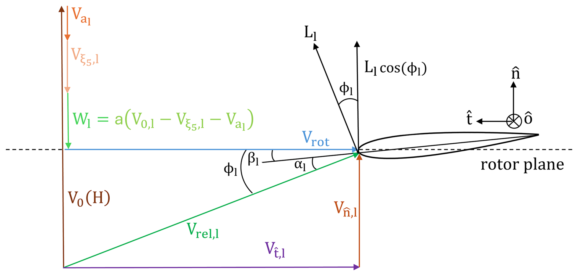
Figure 2 The airfoil velocity triangle expressed in a coordinate system composed of a tangential ($\widehat{t}$), normal ($\widehat{n}$), and outward ($\widehat{o}$) unit vector.

From Fig. 2, several geometric relations are inferred, and one of them is simply $V_{\mathrm{rel},l}^{\mathrm{2}}=V_{\widehat{n},l}^{\mathrm{2}}+V_{\widehat{t},l}^{\mathrm{2}}$. The relative velocity V_rel,l has an orientation which is given by the inflow angle ϕ_l and the following trigonometric relation: ${\mathit{\varphi }}_l={\tan }^{-\mathrm{1}}\left(-V_{\widehat{n},l}/V_{\widehat{t},l}\right)$. The inflow angle ϕ_l is also described as the sum of the twist angle β_l with the angle of attack α_l, which reads as ${\mathit{\varphi }}_l={\mathit{\alpha }}_l+{\mathit{\beta }}_l$.

Besides, the relative velocity V_rel,l is affected by the wake velocity W_l. The induced wake velocity W_l has only a velocity component that is orientated in the normal direction to the rotor plane, and it is characterized by the induction factor a. On this basis, the radial and tangential velocity to the rotor plane, $V_{\widehat{t},l}$, is the rotational velocity $V_{\mathrm{rot}}=-\mathrm{\Omega }d$ at r=d. The contribution from the rotational wake induction factor a^′ is negligible and hence chosen to be ignored in this analysis, meaning that $V_{\widehat{t},l}=V_{\mathrm{rot}}$.

The velocity $V_{\widehat{n},l}$, normal to the rotor plane, is influenced by the inflow velocity V₀, by the velocity perceived on the airfoil due to the blade deflection $V_{a_l}$, and by the velocity caused by the floater's pitch angular motion $V_{{\mathit{\xi }}_{\mathrm{5}},l}$. This leads to

$$\begin{array}{}\text{(18)}& V_{\widehat{n},l}=\left(\mathrm{1}-a\right)\left(V_{\mathrm{0}}\left(H\right)-\underset{V_{{\mathit{\xi }}_{\mathrm{5}},l}}{\underbrace{\dot{{\mathit{\xi }}_{\mathrm{5}}}\left(H+d\cos {\mathrm{\Psi }}_l\right)}}-\underset{V_{a_l}}{\underbrace{{\dot{a}}_l{\mathit{\varphi }}_{\mathrm{1}\mathrm{f}}\left(d\right)}}\right).\end{array}$$

2.2.2 Linearization of aerodynamic loads

Given Eq. (18), $V_{\widehat{n},l}^{\mathrm{2}}$ is expanded as

$$\begin{array}{}\text{(19)}& \begin{array}{rl}{V}_{\widehat{n},l}^{\mathrm{2}}& =\underset{\text{steady term}}{\underbrace{{\left(\mathrm{1}-a\right)}^{\mathrm{2}}{V}_{\mathrm{0}}^{\mathrm{2}}\left(H\right)}}\\ & +\underset{\text{higher-order terms neglected}}{\underbrace{{\left(\mathrm{1}-a\right)}^{\mathrm{2}}\left(\mathrm{2}{\dot{\mathit{\xi }}}_{\mathrm{5}}\left(H+d\cos {\mathrm{\Psi }}_l\right){\dot{a}}_l{\mathit{\varphi }}_{\mathrm{1}\mathrm{f}}\left(d\right)+{\dot{\mathit{\xi }}}_{\mathrm{5}}^{\mathrm{2}}{\left(H+d\cos {\mathrm{\Psi }}_l\right)}^{\mathrm{2}}+{\dot{a}}_l^{\mathrm{2}}{\left({\mathit{\varphi }}_{\mathrm{1}\mathrm{f}}\left(d\right)\right)}^{\mathrm{2}}\right)}}\\ & +\underset{\text{damping contribution}}{\underbrace{\mathrm{2}{\left(\mathrm{1}-a\right)}^{\mathrm{2}}{V}_{\mathrm{0}}\left(H\right)\left(-\dot{{\mathit{\xi }}_{\mathrm{5}}}\left(H+d\cos {\mathrm{\Psi }}_l\right)-{\dot{a}}_l{\mathit{\varphi }}_{\mathrm{1}\mathrm{f}}\left(d\right)\right)}}.\end{array}\end{array}$$

For linearization purposes, higher-order terms of $V_{\widehat{n},l}^{\mathrm{2}}$ are neglected in the derivations to come.

Using the previous aerodynamic identities, the lift force L_l is projected in the normal direction to the rotor plane as can be seen in Fig. 2. This projection is done by utilizing the inflow angle ϕ_l:

$$\begin{array}{}\text{(20)}& F_l=L_l\cos {\mathit{\varphi }}_l.\end{array}$$

The aerodynamic load F_l is a driver of the floating wind turbine's motion. It is linearized as

$$\begin{array}{}\text{(21)}& \begin{array}{rl}& {\displaystyle \frac{\partial \left(L_{l,\mathrm{lin}}\cos {\mathit{\varphi }}_{l,\mathrm{lin}}\right)}{\partial \cdot }}={\displaystyle \frac{\mathrm{1}}{\mathrm{2}}}\mathit{\rho }c\\ & \times \left({\left.{\displaystyle \frac{\partial C_{L,l}}{\partial \cdot }}\right|}_{\mathrm{st}}\cos {\mathit{\varphi }}_{\mathrm{st}}{V}_{\mathrm{rel},\mathrm{st}}^{\mathrm{2}}+C_{L,\mathrm{st}}{\left.{\displaystyle \frac{\partial \cos {\mathit{\varphi }}_{l,\mathrm{lin}}}{\partial \cdot }}\right|}_{\mathrm{st}}{V}_{\mathrm{rel},\mathrm{st}}^{\mathrm{2}}\right.\\ & \left.+C_{L,\mathrm{st}}\cos {\mathit{\varphi }}_{\mathrm{st}}{\left.{\displaystyle \frac{\partial \left(V_{\mathrm{rel},l}^{\mathrm{2}}\right)}{\partial \cdot }}\right|}_{\mathrm{st}}\right),\end{array}\end{array}$$

where the label st represents the steady-state value of a variable. In Eq. (21), the variables $C_{L,l,\mathrm{lin}}$, cos ϕ_l,lin, and $V_{\mathrm{rel},l,\mathrm{lin}}^{\mathrm{2}}$ are linearized in the same fashion as Y_l,lin,

$$\begin{array}{}\text{(22)}& \begin{array}{rl}{Y}_{l,\mathrm{lin}}& =Y_{l,st}+\mathrm{\Delta }Y=Y_{l,st}+{\left.{\displaystyle \frac{\partial Y_l}{\partial {\dot{a}}_l}}\right|}_{\mathrm{st}}{\dot{a}}_l+{\left.{\displaystyle \frac{\partial Y_l}{\partial f_{\mathrm{s},l}}}\right|}_{\mathrm{st}}\\ & \times f_{\mathrm{s},l}+{\left.{\displaystyle \frac{\partial Y_l}{\partial {\dot{\mathit{\xi }}}_{\mathrm{5}}}}\right|}_{\mathrm{st}}{\dot{\mathit{\xi }}}_{\mathrm{5}}.\end{array}\end{array}$$

The linearization contribution ${\left.\frac{\partial Y_l}{\partial f_{\mathrm{s},l}}\right|}_{\mathrm{st}}{f}_{\mathrm{s},l}$ that pertains to the dynamic stall variable f_s will be introduced later in the dynamic stall subsection. For the linearization of L_l,lin, one consideration required to be taken into account is that $V_{\widehat{t},l}$ is constant, which entails that

$$\begin{array}{}\text{(23)}& {\displaystyle \frac{\partial V_{\mathrm{rel},l}^{\mathrm{2}}}{\partial \cdot }}={\displaystyle \frac{\partial V_{\widehat{n},l}^{\mathrm{2}}}{\partial \cdot }}.\end{array}$$

For the development of the linear model, using Eq. (21), it can be demonstrated that the partial derivative of $V_{\widehat{n},l}$ is involved in the linearization of the force F_l. The partial derivative of $V_{\widehat{n},l}$ appears notably when deriving the inflow angle ϕ_l with respect to other variables as

$$\begin{array}{}\text{(24)}& {\displaystyle \frac{\partial {\mathit{\varphi }}_l}{\partial \cdot }}={\displaystyle \frac{\mathrm{1}}{-V_{\widehat{t},\mathrm{st}}\left(\frac{V_{\widehat{n},\mathrm{st}}^{\mathrm{2}}}{V_{\widehat{t},\mathrm{st}}^{\mathrm{2}}}+\mathrm{1}\right)}}{\displaystyle \frac{\partial V_{\widehat{n},l}}{\partial \cdot }}.\end{array}$$

The partial derivative of the lift coefficient C_L,l is dependent on the angle of attack α_l and the dynamic stall variable f_s,l. Details related to the dynamic stall lift coefficient are clarified later in the paper. Hence, it remains to analyse for the linear model the partial derivative of cos ϕ_l, which is found to be

$$\begin{array}{}\text{(25)}& {\displaystyle \frac{\partial \cos {\mathit{\varphi }}_l}{\partial \cdot }}=-{\displaystyle \frac{V_{\widehat{n},\mathrm{st}}}{V_{\widehat{t},\mathrm{st}}^{\mathrm{2}}{\left(\frac{V_{\widehat{n},\mathrm{st}}^{\mathrm{2}}}{V_{\widehat{t},\mathrm{st}}^{\mathrm{2}}}+\mathrm{1}\right)}^{\frac{\mathrm{3}}{\mathrm{2}}}}}{\displaystyle \frac{\partial V_{\widehat{n},l}}{\partial \cdot }}.\end{array}$$

The aerodynamic forcing terms from Eqs. (8) and (9) are linearized as GF${}_{a_l,\mathrm{lin}}=F_{l,\mathrm{lin}}{L}_{\mathrm{b}}{\mathit{\varphi }}_{\mathrm{1}\mathrm{f}}\left(d\right)$ and $M_{\mathrm{aero},\mathrm{lin}}={\sum }_{l=\mathrm{1}}^{N_{\mathrm{b}}}{F}_{l,\mathrm{lin}}{L}_{\mathrm{b}}\left(H+d\cos {\mathrm{\Psi }}_l\right)$ through the linearization of variables $C_{L,l,\mathrm{lin}}$, cos ϕ_l,lin, and $V_{\mathrm{rel},l,\mathrm{lin}}^{\mathrm{2}}$ as shown in Eq. (21).

We can now build a linearized model, characterized by the index L, for use in the stability analysis. For that to occur, a part of the aerodynamic loading from F_T in Eq. (9) is moved from the right-hand side to the left-hand side and then linearized in the form of an added aerodynamic damping matrix contribution noted C_A,

$$\begin{array}{}\text{(26)}& {\mathbf{M}}_S\ddot{\mathit{x}}+\left({\mathbf{C}}_S+{\mathbf{C}}_A\right)\dot{\mathit{x}}+{\mathbf{K}}_S\mathit{x}={\mathit{F}}_L.\end{array}$$

In the EOM from Eq. (26) which pertains to the linearized model, the damping matrix is altered due to the added linearized aerodynamic damping matrix C_A consideration. The partial derivatives of the forcing variables M_aero,lin and GF${}_{a,l,lin}$ allow us to put together that linearized aerodynamic damping matrix contribution C_A as

$$\begin{array}{}\text{(27)}& {\mathbf{C}}_A={\left[\begin{array}{cccc}-\frac{\partial M_{\mathrm{aero},\mathrm{lin}}}{\partial {\dot{\mathit{\xi }}}_{\mathrm{5}}}& -\frac{\partial M_{\mathrm{aero},\mathrm{lin}}}{\partial {\dot{a}}_{\mathrm{1}}}& -\frac{\partial M_{\mathrm{aero},\mathrm{lin}}}{\partial {\dot{a}}_{\mathrm{2}}}& -\frac{\partial M_{\mathrm{aero},\mathrm{lin}}}{\partial {\dot{a}}_{\mathrm{3}}}\\ -\frac{\partial {\mathrm{GF}}_{a_{\mathrm{1}},\mathrm{lin}}}{\partial {\dot{\mathit{\xi }}}_{\mathrm{5}}}& -\frac{\partial {\mathrm{GF}}_{a_{\mathrm{1}},\mathrm{lin}}}{\partial {\dot{a}}_{\mathrm{1}}}& \mathrm{0}& \mathrm{0}\\ -\frac{\partial {\mathrm{GF}}_{a_{\mathrm{2}},\mathrm{lin}}}{\partial {\dot{\mathit{\xi }}}_{\mathrm{5}}}& \mathrm{0}& -\frac{\partial {\mathrm{GF}}_{a_{\mathrm{2}},\mathrm{lin}}}{\partial {\dot{a}}_{\mathrm{2}}}& \mathrm{0}\\ -\frac{\partial {\mathrm{GF}}_{a_{\mathrm{3}},\mathrm{lin}}}{\partial {\dot{\mathit{\xi }}}_{\mathrm{5}}}& \mathrm{0}& \mathrm{0}& -\frac{\partial {\mathrm{GF}}_{a_{\mathrm{3}},\mathrm{lin}}}{\partial {\dot{a}}_{\mathrm{3}}}\end{array}\right]}_{\mathrm{st}}.\end{array}$$

The partial derivatives within C_A are all evaluated at steady-state (st) conditions for the linear model, given an operational point with a specific rotational speed Ω and inflow velocity V₀.

2.2.3 Dynamic stall model

To evaluate the stability of a floating wind turbine model with aerodynamic states, we include a dynamic stall model. The variation of the angle of attack on an airfoil does not immediately impact the aerodynamic lift and drag forces due to the inertia, resulting in a time delay. Due to its simple implementation, we decided to include Øye's dynamic stall model (Øye, 1991) which does take into account the time delay effect on aerodynamic loads. According to Øye's model, the dynamic stall can be expressed in the lift coefficient C_L through the flow separation function variable f_s. The variable f_s indicates the trailing-edge flow separation point location x, starting from the leading edge, as a ratio with respect to chord length, i.e. $f_{\mathrm{s}}=x/c$ (Øye, 1991). The value of f_s=1 corresponds to stall not occurring, signifying that the flow remains fully attached. On the contrary, a value of f_s=0 implies that the separation occurs at the leading edge of the airfoil and that the flow is actually fully separated. According to Øye's dynamic stall model, the influence of f_s on the lift coefficient C_L is

$$\begin{array}{}\text{(28)}& C_L\left({\mathit{\alpha }}_l,f_{\mathrm{s}}\right)=f_{\mathrm{s}}{C}_{L,\mathrm{inv}}\left({\mathit{\alpha }}_l\right)+\left(\mathrm{1}-f_{\mathrm{s}}\right)C_{L,\mathrm{stall}}\left({\mathit{\alpha }}_l\right).\end{array}$$

In this context, C_L,inv(α) refers to the inviscid or fully attached flow lift coefficient, whereas C_L,stall(α) relates to a fully separated flow. Considering that the angle of attack value α would be known, both lift coefficients C_L,inv(α) and C_L,stall(α) are determined by the airfoil data from Fig. 3. For the linearization of C_L from Eq. (28), a set of partial derivatives are established, including $\frac{\partial C_{L,l}}{\partial {\mathit{\alpha }}_l}$ and $\frac{\partial C_{L,l}}{\partial f_{\mathrm{s},l}}$, respectively, as

$$\begin{array}{}\text{(29)}& \begin{array}{rl}{\displaystyle \frac{\partial C_{L,l}}{\partial {\mathit{\alpha }}_l}}& =f_{\mathrm{s}}{\left.{\displaystyle \frac{\partial C_{L,\mathrm{inv},l}}{\partial {\mathit{\alpha }}_l}}\right|}_{\mathrm{st}}+\left(\mathrm{1}-f_{\mathrm{s}}\right){\left.{\displaystyle \frac{\partial C_{L,\mathrm{stall},l}}{\partial {\mathit{\alpha }}_l}}\right|}_{\mathrm{st}}\\ & \text{and}{\displaystyle \frac{\partial C_{L,l}}{\partial f_{\mathrm{s},l}}}={\left.C_{L,\mathrm{inv}}\left({\mathit{\alpha }}_l\right)\right|}_{\mathrm{st}}-{\left.C_{L,\mathrm{stall}}\left({\mathit{\alpha }}_l\right)\right|}_{\mathrm{st}}.\end{array}\end{array}$$

By making use of the airfoil data from Fig. 3, the values of ${\left.\frac{\partial C_{L,\mathrm{inv},l}}{\partial {\mathit{\alpha }}_l}\right|}_{\mathrm{st}}$ and ${\left.\frac{\partial C_{L,\mathrm{stall},l}}{\partial {\mathit{\alpha }}_l}\right|}_{\mathrm{st}}$ are computed numerically as gradients at the operational angle of attack α_l through a cubic spline interpolation. Lastly, to fill out the linear model's aerodynamic damping matrix C_A according to Eq. (21), the partial derivative of the lift coefficient C_L,l with respect to $\dot{\mathit{x}}={\left[{\dot{\mathit{\xi }}}_{\mathrm{5}},{\dot{a}}_{\mathrm{1}},{\dot{a}}_{\mathrm{2}},{\dot{a}}_{\mathrm{3}}\right]}^{\mathrm{T}}$ is elucidated by using the previous partial derivative identity from Eq. (24):

$$\begin{array}{}\text{(30)}& {\displaystyle \frac{\partial C_{L,l}}{\partial \cdot }}={\displaystyle \frac{\partial C_{L,l}}{\partial {\mathit{\alpha }}_l}}{\displaystyle \frac{\partial {\mathit{\alpha }}_l}{\partial \cdot }}={\displaystyle \frac{\partial C_{L,l}}{\partial {\mathit{\alpha }}_l}}{\displaystyle \frac{\partial {\mathit{\varphi }}_l}{\partial \cdot }}.\end{array}$$

The linearization of C_L with respect to f_s is next included in the forcing vector F_T from the time domain model and in F_L from the linear model as

$$\begin{array}{}\text{(31)}& \begin{array}{rl}& {\mathit{F}}_T=\left[\begin{array}{c}{M}_{\mathrm{aero}}+M_{\mathrm{F}}={\sum }_{l=\mathrm{1}}^{\mathrm{3}}{L}_{\mathrm{b}}\left(H+d\cos {\mathrm{\Psi }}_l\right)\\ \cdot \left(\frac{\mathrm{1}}{\mathrm{2}}\mathit{\rho }c\left(\frac{\partial C_{L,l}}{\partial f_{\mathrm{s},l}}{f}_{\mathrm{s},l}+C_{L,\mathrm{stall},l}\right)\cos {\mathit{\varphi }}_{\mathrm{st}}{V}_{\mathrm{rel},\mathrm{st}}^{\mathrm{2}}\right)+M_{\mathrm{F}}\\ {\mathrm{GF}}_{a,\mathrm{1},\mathrm{lin}}=L_{\mathrm{b}}{\mathit{\varphi }}_{\mathrm{1}\mathrm{f}}\left(d\right)\left(\frac{\mathrm{1}}{\mathrm{2}}\mathit{\rho }c\left(\frac{\partial C_{L,\mathrm{1}}}{\partial f_{\mathrm{s},\mathrm{1}}}{f}_{\mathrm{s},\mathrm{1}}+C_{L,\mathrm{stall},\mathrm{1}}\right)\cos {\mathit{\varphi }}_{\mathrm{st}}{V}_{\mathrm{rel},\mathrm{st}}^{\mathrm{2}}\right)\\ \mathrm{⋮}\end{array}\right]\\ & {\mathit{F}}_L=\left[\begin{array}{c}{\sum }_{l=\mathrm{1}}^{\mathrm{3}}{L}_{\mathrm{b}}\left(H+\mathrm{d}\cos {\mathrm{\Psi }}_l\right)\cdot \left(\frac{\mathrm{1}}{\mathrm{2}}\mathit{\rho }c\left({\left.\frac{\partial C_{L,l}}{\partial f_{\mathrm{s},l}}\right|}_{\mathrm{st}}{f}_{\mathrm{s},l}\right)\cos {\mathit{\varphi }}_{\mathrm{st}}{V}_{\mathrm{rel},\mathrm{st}}^{\mathrm{2}}\right)+M_{\mathrm{F}}\\ L_{\mathrm{b}}{\mathit{\varphi }}_{\mathrm{1}\mathrm{f}}\left(d\right)\left(\frac{\mathrm{1}}{\mathrm{2}}\mathit{\rho }c\left({\left.\frac{\partial C_{L,\mathrm{1}}}{\partial f_{\mathrm{s},\mathrm{1}}}\right|}_{\mathrm{st}}{f}_{\mathrm{s},\mathrm{1}}\right)\cos {\mathit{\varphi }}_{\mathrm{st}}{V}_{\mathrm{rel},\mathrm{st}}^{\mathrm{2}}\right)\\ \mathrm{⋮}\end{array}\right].\end{array}\end{array}$$

The time domain model forcing vector F_T considers a linear f_s contribution through a C_L variation dictated by Eq. (28). Because the aerodynamic damping force is included in F_T, what remains from it in F_L is only the contribution of the partial derivative ${\left.\frac{\partial C_{L,l}}{\partial f_{\mathrm{s},l}}\right|}_{\mathrm{st}}={\left.C_{L,\mathrm{inv}}\right|}_{\mathrm{st}}-{\left.C_{L,\mathrm{stall}}\right|}_{\mathrm{st}}$, which is expressed as a constant gradient evaluated at the operational point's steady-state condition. Knowing the identities for F_T and F_L as well as C_L's linearized formulation, a Jacobian matrix of partial derivatives can be derived for both forcing vectors F at each ith row, F_i. The Jacobian matrix of partial derivatives for F_i with respect to f_s,j on the jth column is identified as $\left[\partial {\mathit{F}}_i/\partial {\mathit{f}}_{\mathrm{s},j}\right]$ and has the following composition:

$$\begin{array}{}\text{(32)}& \left[\partial {\mathit{F}}_i/\partial {\mathit{f}}_{\mathrm{s},j}\right]=\left[\begin{array}{ccc}\frac{\partial M_{\mathrm{aero},\mathrm{lin}}}{\partial f_{\mathrm{s},\mathrm{1}}}& \frac{\partial M_{\mathrm{aero},\mathrm{lin}}}{\partial f_{\mathrm{s},\mathrm{2}}}& \frac{\partial M_{\mathrm{aero},\mathrm{lin}}}{\partial f_{\mathrm{s},\mathrm{3}}}\\ \frac{\partial G{F}_{a_{\mathrm{1}},\mathrm{lin}}}{\partial f_{\mathrm{s},\mathrm{1}}}& \mathrm{0}& \mathrm{0}\\ \mathrm{0}& \frac{\partial G{F}_{a_{\mathrm{2}},\mathrm{lin}}}{\partial f_{\mathrm{s},\mathrm{2}}}& \mathrm{0}\\ \mathrm{0}& \mathrm{0}& \frac{\partial G{F}_{a_{\mathrm{3}},\mathrm{lin}}}{\partial f_{\mathrm{s},\mathrm{3}}}\end{array}\right],\end{array}$$

with its assembly directly influenced by the partial derivative $\frac{\partial C_{L,i}}{\partial f_{\mathrm{s},j}}$. For the time domain model, the Jacobian matrix $\left[\partial {\mathit{F}}_i/\partial {\mathit{f}}_{\mathrm{s},j}\right]$ varies in time as the simulation progresses. On the contrary, for the linear model case, $\left[\partial {\mathit{F}}_i/\partial {\mathit{f}}_{\mathrm{s},j}\right]$ is constant and affected by aerodynamic parameters that are fixed at steady-state values found for a given operational point with a particular inflow velocity V₀ and rotational speed Ω.

To be able to compute the lift coefficient C_L that influences the aerodynamic loading, a dynamic stall ordinary differential equation (ODE) for f_s is defined as

$$\begin{array}{}\text{(33)}& {\dot{f}}_{\mathrm{s},l}={\displaystyle \frac{f_{\mathrm{s},\mathrm{static},l}-f_{\mathrm{s},l}}{\mathit{\tau }}}.\end{array}$$

Here τ identifies a steady-state time constant which is inversely proportional to the steady-state relative velocity but directly proportional to the chord length, $\mathit{\tau }=\left(\mathrm{4}c\right)/V_{\mathrm{rel},\mathrm{st}}$. In agreement with previous explanations about stall occurrence, the static value of f_s, i.e. f_s,static, reaches 0 when there is a full separation of the flow. Simultaneously, the dynamic stall contribution to C_L, called C_L,stall(α), reaches then a maximum value. The effects of stall-induced aerodynamic fluctuations are most observable when the static lift coefficient C_L,static curve reaches a maximum value, and then f_s,static is close to 0.5 for the current airfoil (being FFA-W3-241). Figure 3 exhibits the relations between the multiple aerodynamic variables that have been introduced.

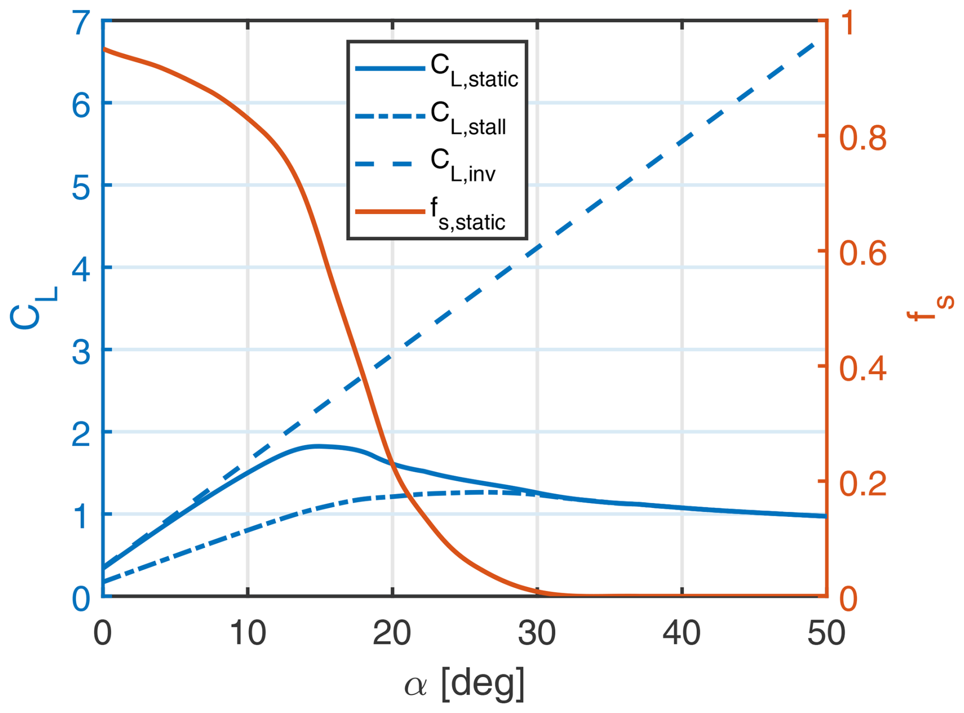
Figure 3 Airfoil FFA-W3-241 dynamic stall data with respect to angle of attack α and is valid at the reference radial position r=d.

In the linearized model, ${\dot{f}}_{\mathrm{s},l}$ is linearized with respect to the four structural DOFs of the system and the three aerodynamic DOFs f_s,l. This requires us to take into account the full linearization of the ${\dot{f}}_{\mathrm{s}}$ ODE by including the linearization of the $f_{\mathrm{s},\mathrm{static},l}$ variable as well,

$$\begin{array}{}\text{(34)}& \begin{array}{rl}{\dot{f}}_{\mathrm{s},l,\mathrm{lin}}& =-{\displaystyle \frac{f_{\mathrm{s},l}}{\mathit{\tau }}}+{\displaystyle \frac{\mathrm{1}}{\mathit{\tau }}}\left({\left.f_{\mathrm{s},\mathrm{static}}\right|}_{\mathrm{st}}+{\left.{\displaystyle \frac{\partial f_{\mathrm{s},\mathrm{static},l}}{\partial {\mathit{\alpha }}_l}}\right|}_{\mathrm{st}}{\left.{\displaystyle \frac{\partial {\mathit{\varphi }}_l}{\partial {\dot{\mathit{\xi }}}_{\mathrm{5}}}}\right|}_{\mathrm{st}}{\dot{\mathit{\xi }}}_{\mathrm{5}}\right.\\ & \left.+{\left.{\displaystyle \frac{\partial f_{\mathrm{s},\mathrm{static},l}}{\partial {\mathit{\alpha }}_l}}\right|}_{\mathrm{st}}{\left.{\displaystyle \frac{\partial {\mathit{\varphi }}_l}{\partial {\dot{a}}_l}}\right|}_{\mathrm{st}}{\dot{a}}_l\right).\end{array}\end{array}$$

This complete linearization translates into the following two Jacobian matrices, represented as

$$\begin{array}{}\text{(35)}& {\left[\partial {\dot{\mathit{f}}}_{\mathrm{s},i}/\partial {\dot{\mathit{x}}}_{\mathrm{4}\times \mathrm{1},j}\right]}_{\mathrm{3}\times \mathrm{4}}={\left[\begin{array}{cccc}\frac{\partial {\dot{f}}_{\mathrm{s},\mathrm{1}}}{\partial {\dot{\mathit{\xi }}}_{\mathrm{5}}}& \frac{\partial {\dot{f}}_{\mathrm{s},\mathrm{1}}}{\partial {\dot{a}}_{\mathrm{1}}}& \mathrm{0}& \mathrm{0}\\ \frac{\partial {\dot{f}}_{\mathrm{s},\mathrm{2}}}{\partial {\dot{\mathit{\xi }}}_{\mathrm{5}}}& \mathrm{0}& \frac{\partial {\dot{f}}_{\mathrm{s},\mathrm{2}}}{\partial {\dot{a}}_{\mathrm{2}}}& \mathrm{0}\\ \frac{\partial {\dot{f}}_{\mathrm{s},\mathrm{3}}}{\partial {\dot{\mathit{\xi }}}_{\mathrm{5}}}& \mathrm{0}& \mathrm{0}& \frac{\partial {\dot{f}}_{\mathrm{s},\mathrm{3}}}{\partial {\dot{a}}_{\mathrm{3}}}\end{array}\right]}_{\mathrm{st}}\end{array}$$

and ${\left[\partial {\dot{\mathit{f}}}_{\mathrm{s},i}/\partial {\mathit{f}}_{\mathrm{s},j}\right]}_{\mathrm{3}\times \mathrm{3}}$, which is a diagonal constant matrix with components on the ith row and jth column being equal to $-\mathrm{1}/\mathit{\tau }$. To evaluate for the linear model the partial derivative ${\left.\frac{\partial f_{\mathrm{s},\mathrm{static},l}}{\partial {\mathit{\alpha }}_l}\right|}_{\mathrm{st}}$ in Eq. (34), the numerical gradient is determined at the corresponding operational angle of attack α_l through the use of the airfoil data from Fig. 3. It is observable in Fig. 4 that the numerical result for the gradient ${\left.\frac{\partial f_{\mathrm{s},\mathrm{static},l}}{\partial {\mathit{\alpha }}_l}\right|}_{\mathrm{st}}$ is calculated via a cubic spline interpolation for a wide range of angles of attack.

Figure 4 Numerical gradient $\partial f_{\mathrm{s},\mathrm{static}}/\partial \mathit{\alpha }$ as a function of the angle of attack α.

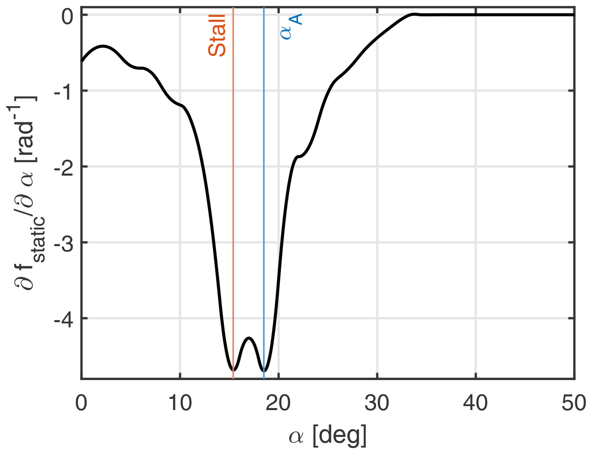
The angle of attack labelled as “Stall” refers to a point in flow separation where C_L,static reaches a maximal value and simultaneously the gradient stops decreasing $\partial f_{\mathrm{s},\mathrm{static}}/\partial \mathit{\alpha }$. The angle of attack α_A identifies the point where the gradient $\partial f_{\mathrm{s},\mathrm{static}}/\partial \mathit{\alpha }$ starts increasing and the end of the transitioning region after the maximal C_L,static value has been reached.

2.3 State-space representation

When combining the time domain model EOM, which is a second-order ODE (see Eq. 10), with the first-order dynamic stall ODE (see Eq. 33), we can rewrite the system as a first-order state-space model. This formulation is comprised of a system matrix A, a state vector q, and a forcing input vector F_B:

$$\begin{array}{}\text{(36)}& \dot{\mathit{q}}=\mathbf{A}\mathit{q}+{\mathit{F}}_B.\end{array}$$

The state vector $\mathit{q}={\left[{\mathit{x}}_{\mathrm{4}\times \mathrm{1}}^{\mathrm{T}},{\dot{\mathit{x}}}_{\mathrm{4}\times \mathrm{1}}^{\mathrm{T}},f_{\mathrm{s},\mathrm{1}},f_{\mathrm{s},\mathrm{2}},f_{\mathrm{s},\mathrm{3}}\right]}^{\mathrm{T}}$ includes the structural DOF vector x, its time derivative $\dot{\mathit{x}}$, and the variable f_s,l for each blade. The length of state q, labelled as N_s, is N_s=11 for a three-bladed wind turbine. The response of q is quantified in terms of variations from the steady-state values, which are determined through simulations using the time domain model. Finally, the state-space system matrix A is built for the time domain model and linearized model, respectively, as

$$\begin{array}{}\text{(37)}& \begin{array}{rl}{\mathbf{A}}_T& =\left[\begin{array}{ccc}\left[{\mathbf{0}}_{\mathrm{4}\times \mathrm{4}}\right]& \left[{\mathbf{I}}_{\mathrm{4}\times \mathrm{4}}\right]& \left[{\mathbf{0}}_{\mathrm{4}\times \mathrm{3}}\right]\\ {\left[-{\mathbf{M}}_S^{-\mathrm{1}}{\mathbf{K}}_S\right]}_{\mathrm{4}\times \mathrm{4}}& {\left[-{\mathbf{M}}^{-\mathrm{1}}{\mathbf{C}}_S\right]}_{\mathrm{4}\times \mathrm{4}}& {\left[{\mathbf{M}}_S^{-\mathrm{1}}\left[\partial {\mathit{F}}_i/\partial {\mathit{f}}_{\mathrm{s},j}\right]\right]}_{\mathrm{4}\times \mathrm{3}}\\ \left[{\mathbf{0}}_{\mathrm{3}\times \mathrm{4}}\right]& \left[{\mathbf{0}}_{\mathrm{3}\times \mathrm{4}}\right]& {\left[\partial {\dot{\mathit{f}}}_{\mathrm{s},i}/\partial {\mathit{f}}_{\mathrm{s},j}\right]}_{\mathrm{3}\times \mathrm{3}}\end{array}\right]\\ {\mathbf{A}}_L& ={\left[\begin{array}{ccc}\left[{\mathbf{0}}_{\mathrm{4}\times \mathrm{4}}\right]& \left[{\mathbf{I}}_{\mathrm{4}\times \mathrm{4}}\right]& \left[{\mathbf{0}}_{\mathrm{4}\times \mathrm{3}}\right]\\ {\left[-{\mathbf{M}}_S^{-\mathrm{1}}{\mathbf{K}}_S\right]}_{\mathrm{4}\times \mathrm{4}}& {\left[-{\mathbf{M}}_S^{-\mathrm{1}}\left({\mathbf{C}}_S+{\mathbf{C}}_A\right)\right]}_{\mathrm{4}\times \mathrm{4}}& {\left[{\mathbf{M}}_S^{-\mathrm{1}}\left[\partial {\mathit{F}}_i/\partial {\mathit{f}}_{\mathrm{s},j}\right]\right]}_{\mathrm{4}\times \mathrm{3}}\\ \left[{\mathbf{0}}_{\mathrm{3}\times \mathrm{4}}\right]& {\left[\partial {\dot{\mathit{f}}}_{\mathrm{s},i}/\partial {\dot{\mathit{x}}}_j\right]}_{\mathrm{3}\times \mathrm{4}}& {\left[\partial {\dot{\mathit{f}}}_{\mathrm{s},i}/\partial {\mathit{f}}_{\mathrm{s},j}\right]}_{\mathrm{3}\times \mathrm{3}}\end{array}\right]}_{\mathrm{st}}.\end{array}\end{array}$$

It is important to recall that the linear model system matrix A_L components are all evaluated at steady-state (st) conditions. In contrast, the time domain model matrix A_T has partial derivatives that vary in time. For simulations with a forced response, the time domain model state-space forcing vector F_B,T is, just like A_T, impacted implicitly by a variation of aerodynamic parameters. On the other hand, the linearized model's forcing vector F_B,L contains only a platform pitch forcing moment M_F contribution because it accounts for a response variation around steady state. This is summarized as

$$\begin{array}{}\text{(38)}& \begin{array}{rl}{\mathit{F}}_{B,T}& =\left[\begin{array}{c}\left[{\mathbf{0}}_{\mathrm{4}\times \mathrm{1}}\right]\\ {\mathbf{M}}_S^{-\mathrm{1}}\left[\begin{array}{c}{\sum }_{l=\mathrm{1}}^{\mathrm{3}}{L}_{\mathrm{b}}\left(H+d\cos {\mathrm{\Psi }}_l\right)\cdot \left(\frac{\mathrm{1}}{\mathrm{2}}\mathit{\rho }c{C}_{L,\mathrm{stall},l}\cos {\mathit{\varphi }}_{\mathrm{st}}{V}_{\mathrm{rel},\mathrm{st}}^{\mathrm{2}}\right)+M_{\mathrm{F}}\\ L_{\mathrm{b}}{\mathit{\varphi }}_{\mathrm{1}\mathrm{f}}\left(d\right)\left(\frac{\mathrm{1}}{\mathrm{2}}\mathit{\rho }c{C}_{L,\mathrm{stall},\mathrm{1}}\cos {\mathit{\varphi }}_{\mathrm{st}}{V}_{\mathrm{rel},\mathrm{st}}^{\mathrm{2}}\right)\\ \mathrm{⋮}\end{array}\right]\\ \left[\begin{array}{c}{f}_{\mathrm{s},\mathrm{static},\mathrm{1}}/\mathit{\tau }\\ f_{\mathrm{s},\mathrm{static},\mathrm{2}}/\mathit{\tau }\\ f_{\mathrm{s},\mathrm{static},\mathrm{3}}/\mathit{\tau }\end{array}\right]\end{array}\right]\\ & {\mathit{F}}_{B,L}=\left[\begin{array}{c}\left[{\mathbf{0}}_{\mathrm{4}\times \mathrm{1}}\right]\\ {\mathbf{M}}_S^{-\mathrm{1}}\left[\begin{array}{c}{M}_{\mathrm{F}}\\ \left[{\mathbf{0}}_{\mathrm{3}\times \mathrm{1}}\right]\end{array}\right]\\ \left[{\mathbf{0}}_{\mathrm{3}\times \mathrm{1}}\right]\end{array}\right].\end{array}\end{array}$$

3 Model verification

After the state-space representation of the time domain model and linear model is completed, time domain simulations are performed to assess how both models function in terms of decay tests and dynamic stall responses. These simulations serve as a model verification as well.

3.1 Decay tests

To verify that the linear model (LM) has been fully linearized and that it behaves in a physically correct manner, decay test simulations are carried out to compare results with the time domain model (TDM). Results are presented as variations from the steady-state values. The simulation conditions consider an operational point of V₀=8 m s⁻¹ and Ω=0.6 rad s⁻¹. The corresponding steady-state angle of attack and lift coefficient are located in a region where the flow is partially attached and close to reaching maximal C_L,static; see Fig. 3. The initial space perturbations for the structural DOFs (ξ₅ and a_l) are equal to the negative value of the steady-state values, and the initial conditions for the dynamic stall f_s,l variables are the corresponding values for those structural DOF initial conditions. This means that ${\mathit{\xi }}_{\mathrm{5}}(t=\mathrm{0})=-\mathrm{0.02}$ rad, $a_l(t=\mathrm{0})=-\mathrm{7.11}$ m, and $f_{\mathrm{s},l}(t=\mathrm{0})=-\mathrm{0.67}$.

The results from Fig. 5 show that the steady-state plateau values for the a_l and the f_s,l signals are reached in a very short time span. The time domain plots also confirm that there is no disparity between the results obtained with the TDM and the LM. Time responses also indicate that the system is highly damped with regards to the a_l and the f_s,l DOFs in comparison to the floater pitch ξ₅, which has not reached its steady-state value yet in the time frame displayed here.

In the frequency domain, the power spectral density (PSD) plots in the right column of Fig. 5 capture at the peaks the natural frequency of the floater pitch motion, ${\mathit{\omega }}_{{\mathit{\xi }}_{\mathrm{5}}}$, for the ξ₅ signal but also the shifted frequencies of $-{\mathit{\omega }}_{{\mathit{\xi }}_{\mathrm{5}}}+\mathrm{\Omega }$ and ${\mathit{\omega }}_{{\mathit{\xi }}_{\mathrm{5}}}+\mathrm{\Omega }$ in the other signals (a_l and f_s,l) because of the system's periodicity. This entails that damped frequencies shifted by ±mΩ, where m is an integer, are also part of the response. The blade natural frequency, ω_1f=0.6255 Hz, cannot be captured by any signal with a decay test due to a very high aerodynamic damping contribution. It was investigated by the authors (Pamfil et al., 2024) that the blade natural frequency was well captured once the aerodynamic damping contribution was numerically reduced by decreasing the air density, ρ.

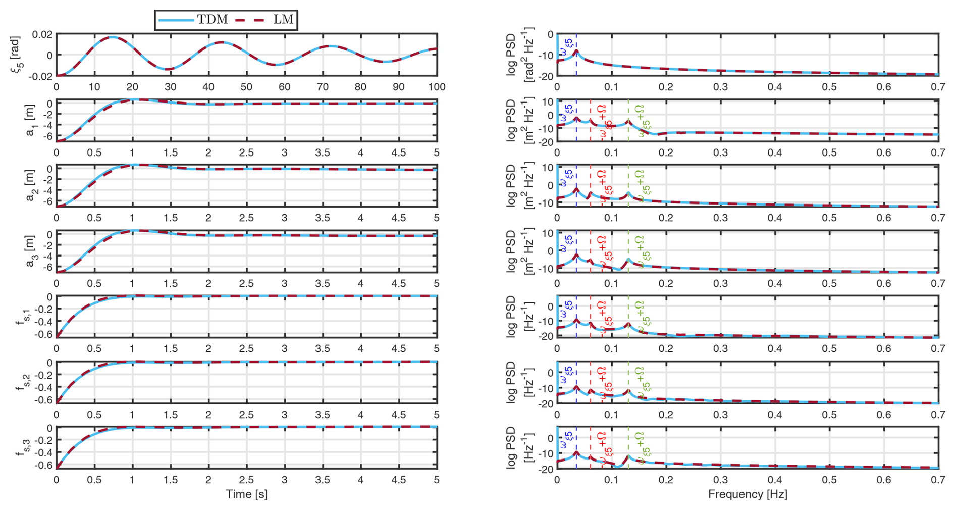
Figure 5 Decay test for the operational point of V₀=8 m s⁻¹, Ω=0.6 rad s⁻¹, and τ=0.34 s, where the TDM and LM results are compared.

3.2 Dynamic stall analysis

To test, furthermore, the correct implementation of the linearized model compared to results generated with the time domain model, we analyse on C_L–α plots the hysteresis behaviour of the airfoil's lift due to the dynamic stall.

3.2.1 Operational point and floater pitch moment variation

The most direct way to verify the C_L–α responses in terms of dynamic stall behaviour is to vary the platform pitch moment M_F that is given by a harmonic time dependence as follows:

$$\begin{array}{}\text{(39)}& M_{\mathrm{F}}=A_M\cos \left({\mathrm{\Omega }}_{M}t\right),\end{array}$$

with amplitude A_M and excitation frequency Ω_M. The amplitude A_M is varied depending on the chosen operational point to achieve the desired angle of attack variation, resulting in the hysteresis behaviour that can be noticeable on C_L–α plots.

Figure 6 reports the TDM and LM results for three operational conditions with the same inflow velocity of V₀=8 m s⁻¹. For each operational point, the floater pitch moment excitation amplitude A_M is changed, whereas its excitation frequency Ω_M is fixed at 0.15 Hz, with Ω_M=0.94 rad s⁻¹. The three operational points that are experimented with are located at the angle of attack corresponding to a maximal value of C_L,static, before, and right after, respectively, to allow us to examine more clearly the hysteresis behaviour for a high fluctuation of the lift and angle of attack values. The results for the point located where the flow is partially attached and before C_L,static is maximal are presented in the first row. These results are achieved with a rotor speed of Ω=0.43 rad s⁻¹ that is below the minimum rotor speed of 6 RPM for the DTU 10 MW reference turbine at V₀=8 m s⁻¹, with a nominal time constant τ_nom=0.47 s and with $A_M=\mathrm{1.212}\times {\mathrm{10}}^{\mathrm{9}}$ Nm. The results presented in the second and third rows in Fig. 6 are related to an operational point located, respectively, at the maximal C_L,static region around α=15 deg and nearby at a higher angle of attack. The simulation conditions for the second and third rows are, respectively, a rotor speed of Ω=0.38 rad s⁻¹ and Ω=0.35 rad s⁻¹, a nominal time constant of τ_nom=0.52 s and τ_nom=0.56 s, and a platform pitch moment amplitude of $A_M=\mathrm{9.70}\times {\mathrm{10}}^{\mathrm{8}}$ Nm and $A_M=\mathrm{1.212}\times {\mathrm{10}}^{\mathrm{9}}$ Nm. The distinction for the three different operational conditions in terms of nominal time constant ${\mathit{\tau }}_{\mathrm{nom}}=\left(\mathrm{4}c\right)/V_{\mathrm{rel},\mathrm{st}}$ arises from the difference in steady-state relative velocity $V_{\mathrm{rel},\mathrm{st}}=\sqrt{V_{\widehat{n},l}^{\mathrm{2}}+V_{\widehat{t},l}^{\mathrm{2}}}$ through the tangential velocity component $V_{\widehat{t},l}=-\mathrm{\Omega }d$; see airfoil velocity triangle in Fig. 2.

Furthermore, the time frame chosen to be plotted entirely captures the steady-state cyclic behaviour of the lift coefficient and angle of attack for more than one cycle.

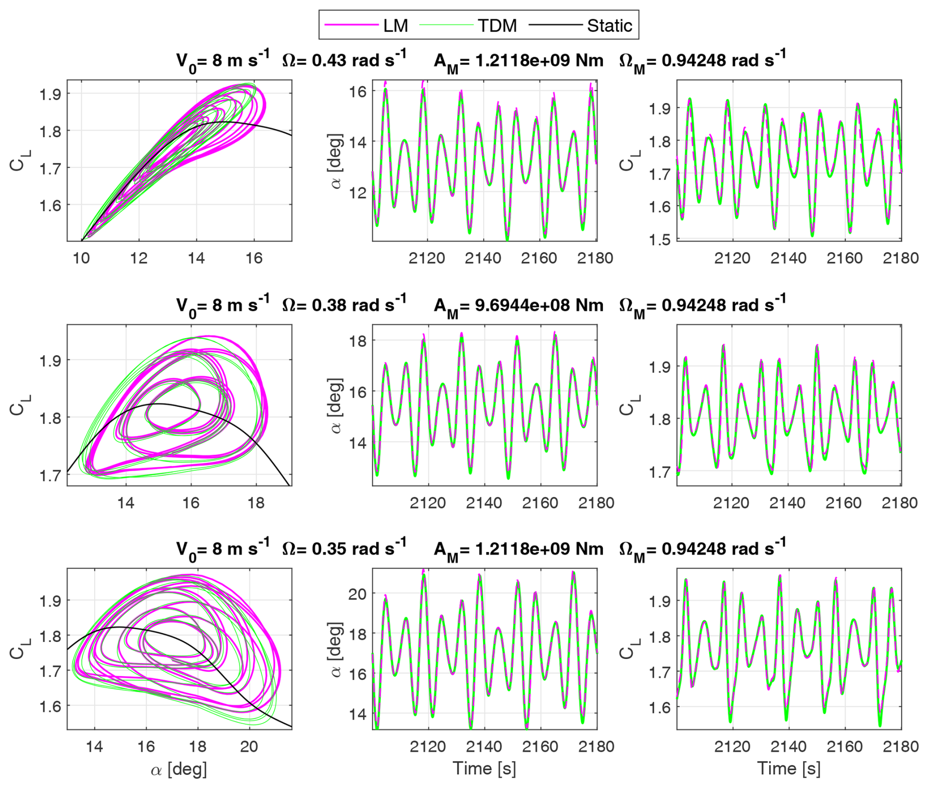
Figure 6 Dynamic lift and stall behaviour at three different operational points surrounding the maximal static lift coefficient C_L,static region, with a varying forcing moment applied on the floater pitch DOF, and where the TDM and LM results are compared.

The hysteresis phenomenon is caused by the time delay effect in the region of the operational point; see airfoil data in Fig. 3. There is a good overall match between the time domain and linear model time series for α and C_L. Both the time domain and linear models are able to describe the stall phenomenon. This difference between results is more pronounced in the region before maximal C_L,static is achieved, where the hysteresis curves are more elongated.

3.2.2 Influence from time constant

The aerodynamic damping depends on the time constant τ from the dynamic stall model, and it influences the behaviour of the system where the flow is partially attached ($\mathrm{1}>f_{\mathrm{s}}>\mathrm{0}$). Varying τ's value in the dynamic stall model with respect to a reference nominal value τ_nom=0.34 s would clarify what the impact is on the angle of attack α and lift coefficient C_L, and it demonstrates the effect on the aerodynamic damping. Simulations are executed at an operational point of V₀=8 m s⁻¹ and Ω=0.6 rad s⁻¹ with a steady-state angle of attack α=8.32 deg. To observe the effect of τ's change on C_L–α graphs, there is a platform pitch forcing applied with fixed parameters for the amplitude, $A_M=\mathrm{1.212}\times {\mathrm{10}}^{\mathrm{9}}$ Nm, and for the excitation frequency set at 0.15 Hz and ${\mathrm{\Omega }}_M=\mathrm{0.15}\cdot \mathrm{2}\mathit{\pi }$ rad s⁻¹. We investigate the hysteresis behaviour of the lift coefficient and angle of attack time series and compare results between the TDM and LM. In Fig. 7, the hysteresis effect is studied for an angle of attack ranging from α=6.47 deg to α=10.11 deg. The dynamic stall τ parameter is varied by factors of 0.15, 1, and 100 when applied to the nominal value τ_nom=0.34 s.

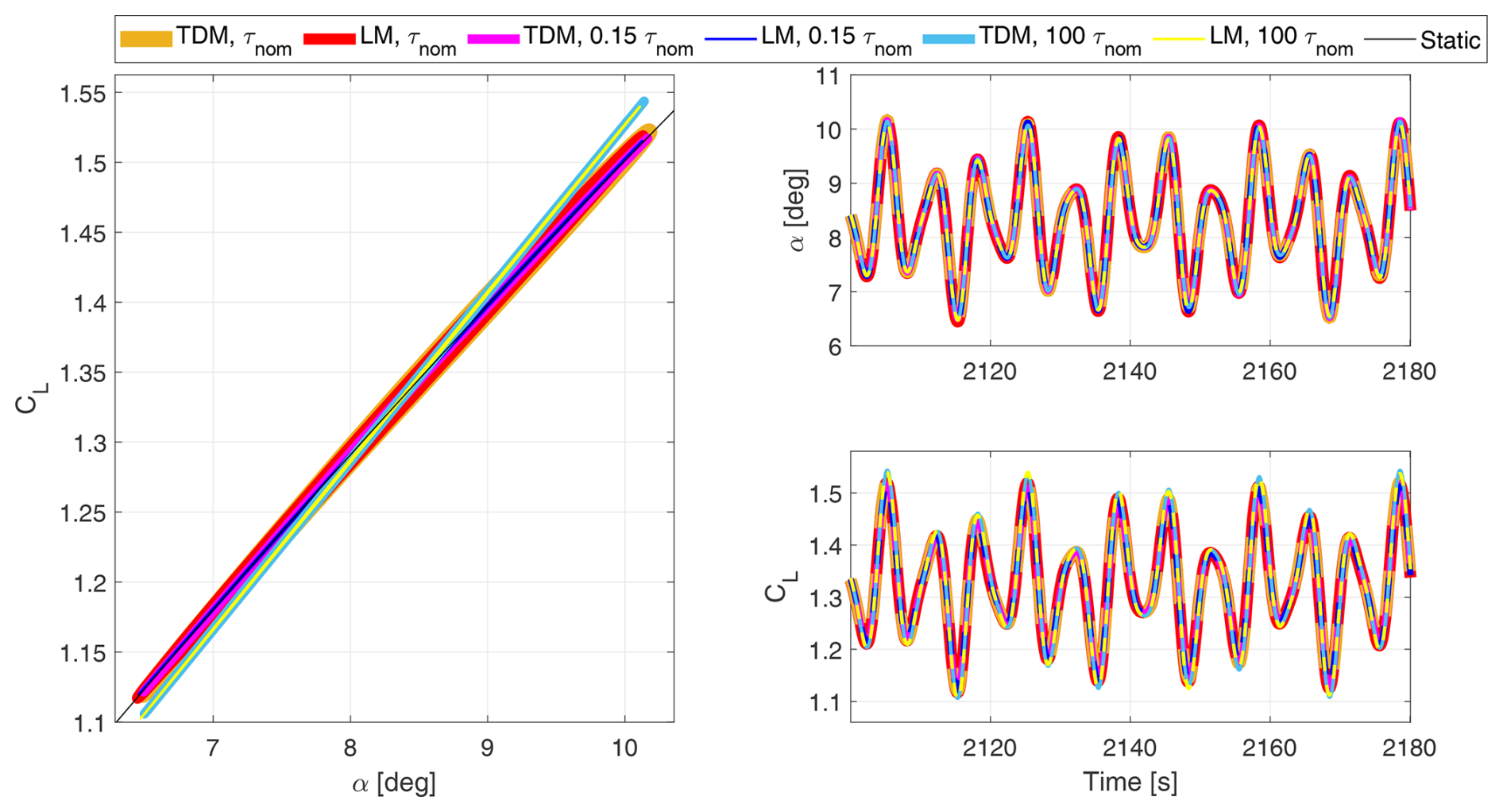
Figure 7 Hysteresis results for simulations with the operational point of V₀=8 m s⁻¹ and Ω=0.6 rad s⁻¹, with a forcing moment applied on the floater pitch DOF, and where TDM and LM results are compared.

The variation of τ's value helps to visualize on a C_L–α plot the impact on the slope $\frac{\partial C_L}{\partial \mathit{\alpha }}$ during the cyclic motion of the platform pitch. Results point out that a higher value of τ brings about a higher slope $\frac{\partial C_L}{\partial \mathit{\alpha }}$. After performing an analytical integration of the ODE from Eq. (33), this conclusion can be supported by studying the influence of τ on the solution of the dynamic stall variable f_s. It is explicitly expressed at a current time step t+Δt for a small time step increment of Δt,

$$\begin{array}{}\text{(40)}& f_{\mathrm{s}}(t+\mathrm{\Delta }t)=f_{\mathrm{s},\mathrm{static}}+\left(f_{\mathrm{s}}\left(t\right)-f_{\mathrm{s},\mathrm{static}}\right)e^{\left(-\frac{\mathrm{\Delta }t}{\mathit{\tau }}\right)}.\end{array}$$

It is discernible in Eq. (40) that a larger time constant τ leads to a larger exponential factor $e^{\left(-\frac{\mathrm{\Delta }t}{\mathit{\tau }}\right)}$. This inevitably increases f_s(t+Δt) through the term $\left(f_{\mathrm{s}}\left(t\right)-f_{\mathrm{s},\mathrm{static}}\right)e^{\left(-\frac{\mathrm{\Delta }t}{\mathit{\tau }}\right)}$. In compliance with Eq. (29) for $\frac{\partial C_L}{\partial \mathit{\alpha }}$, a greater value of f_s induces a higher slope $\frac{\partial C_L}{\partial \mathit{\alpha }}$. To recapitulate, τ's variation has an outcome that is noticeable on a C_L–α graph when a harmonic floater pitch moment is applied. It has been proven that an increased time constant τ produces a higher slope of the lift coefficient C_L over the angle of attack α, which is evidently demonstrated in Fig. 7.

This lift slope trend with an increasing time constant τ in the region where the flow is partially separated is not physically accurate. A dynamic stall model that includes the Theodorsen effect would typically predict a lower effective lift slope at this steady-state angle of attack α=8.32 deg; see, for example, Figs. 8 to 10 in Hansen et al. (2004). The increased lift slope observed in Fig. 7 occurs because Stig Øye's dynamic stall model does not take into account the shed vorticity from the airfoil trailing edge which is modelled by Theodorsen's analytical function. This effect is captured by the Beddoes–Leishman dynamic stall model (Leishman et al., 1986), which was linearized in the form of a state-space model by Hansen et al. (2004). We opted for the Stig Øye dynamic stall model instead because it only requires one aerodynamic stall variable per blade compared to four variables for the Beddoes–Leishman state-space model (Hansen et al., 2004). This alleviates the implementation and linearization of the dynamic stall model equations in the system state-space formulation.

4 Hill's method of infinite determinants

The damping of dynamic systems is usually quantified through the eigenvalue analysis of linearized system matrices. However, for the dynamic system at hand, several system matrix components are azimuthally periodic, meaning that the stability analysis cannot be directly analysed for the time-varying system matrix. Hill's method is a solution that renders the system matrix LTI so that the eigenvalues can be calculated.

4.1 Aero-elastic stability within Hill's method

To obtain an LTI system via Hill's method, the state-space ODE from Eq. (36) is rewritten as a truncated double-sided Fourier series with a summation index ranging from $j=-N$ to N, with N being the upper limit for the expansion. The Fourier series expansion for the state vector q, the time derivative vector $\dot{\mathit{q}}$, and the linearized system matrix A_L (Christensen and Santos, 2005), which are all of dimension N_s, is, respectively,

$$\begin{array}{ll}{\displaystyle }\mathit{q}\left(t\right)& {\displaystyle }=\sum _{j=-N}^N{\mathit{q}}_j\left(t\right)e^{ij\mathrm{\Omega }t},\\ {\displaystyle }\dot{\mathit{q}}\left(t\right)& {\displaystyle }=\sum _{j=-N}^N\left(\left(ij\mathrm{\Omega }\right){\mathit{q}}_j\left(t\right)+{\dot{\mathit{q}}}_j\left(t\right)\right)e^{ij\mathrm{\Omega }t},\text{and}\\ \text{(41)}& {\displaystyle }{\mathbf{A}}_L\left(t\right)& {\displaystyle }=\sum _{j=-N}^N{\mathbf{A}}_{L,j}{e}^{ij\mathrm{\Omega }t},\end{array}$$

where each A_L,j is a constant matrix and where $i=\sqrt{-\mathrm{1}}$. In our model, a Fourier decomposition with N=4 suffices to create an exact description of the system's periodicity.

The Fourier decomposition of the system must be double-sided because the linearized model's system matrix A_L is real and has no imaginary component; refer to Eq. (37). To rephrase, the double-sided Fourier decomposition of A_L allows us to cancel out the imaginary parts that appear from the positive (+jΩ) and negative (−jΩ) harmonics. The expressions from Eq. (41) can be inserted into the state-space ODE from Eq. (36). For the eigenvalue analysis to be applicable, the free vibration condition is considered in Eq. (36), which implies that no input forcing F_B is exerted on the system. This approach is laid out as

$$\begin{array}{}\text{(42)}& \sum _{n=-N}^N\left({\dot{\mathit{q}}}_n\left(t\right)+\left(in\mathrm{\Omega }\right){\mathit{q}}_n\right)e^{in\mathrm{\Omega }t}=\sum _{j=-N}^N\sum _{p=-N}^N{\mathbf{A}}_{L,j}{\mathit{q}}_p{e}^{i\left(j+p\right)\mathrm{\Omega }t}.\end{array}$$

The expression from Eq. (42) can then be manipulated to get

$$\begin{array}{}\text{(43)}& \sum _{n=-N}^N{\dot{\mathit{q}}}_n\left(t\right)e^{in\mathrm{\Omega }t}=\sum _{n=-N}^N\left(-\left(in\mathrm{\Omega }\right){\mathit{q}}_n+\sum _{j=n-N}^{n+N}{\mathbf{A}}_{L,j}{\mathit{q}}_{n-j}\right)e^{in\mathrm{\Omega }t}.\end{array}$$

Since Eq. (43) must hold for any value of time t, the factor for each e^inΩt term in the summation must satisfy

$$\begin{array}{}\text{(44)}& {\dot{\mathit{q}}}_n\left(t\right)=-\left(in\mathrm{\Omega }\right){\mathit{q}}_n+\sum _{j=n-N}^{n+N}{\mathbf{A}}_{L,j}{\mathit{q}}_{n-j}.\end{array}$$

Upon definition of $\widehat{\mathit{q}}=[{\mathit{q}}_{n=-N}^{\mathrm{T}},\mathrm{\dots },{\mathit{q}}_{n=\mathrm{0}}^{\mathrm{T}},\mathrm{\dots },{\mathit{q}}_{n=N}^{\mathrm{T}}{]}^{\mathrm{T}}$, Eq. (44) is recast into a hyper-matrix formulation by varying the index n from −N until N to represent a state-space equation for different harmonics q_n of the response q,

$$\begin{array}{ll}{\displaystyle }\widehat{\dot{\mathit{q}}}& {\displaystyle }=\widehat{\mathbf{A}}\widehat{\mathit{q}},\\ {\displaystyle }\widehat{\mathbf{A}}& {\displaystyle }=\left[\begin{array}{ccccc}\mathrm{\ddots }& \mathrm{⋮}& \mathrm{⋮}& \mathrm{⋮}& \mathrm{\ddots }\\ \mathrm{\dots }& {\mathbf{A}}_{L,\mathrm{0}}+i\mathrm{\Omega }\mathbf{I}& {\mathbf{A}}_{L,-\mathrm{1}}& {\mathbf{A}}_{L,-\mathrm{2}}& \mathrm{\dots }\\ \mathrm{\dots }& {\mathbf{A}}_{L,\mathrm{1}}& {\mathbf{A}}_{L,\mathrm{0}}& {\mathbf{A}}_{L,-\mathrm{1}}& \mathrm{\dots }\\ \mathrm{\dots }& {\mathbf{A}}_{L,\mathrm{2}}& {\mathbf{A}}_{L,\mathrm{1}}& {\mathbf{A}}_{L,\mathrm{0}}-i\mathrm{\Omega }\mathbf{I}& \mathrm{\dots }\\ \mathrm{\ddots }& \mathrm{⋮}& \mathrm{⋮}& \mathrm{⋮}& \mathrm{\ddots }\end{array}\right],\\ \text{(45)}& {\displaystyle }\widehat{\mathit{q}}& {\displaystyle }=\left[\begin{array}{c}\mathrm{⋮}\\ {\mathit{q}}_{n=-\mathrm{1}}\\ {\mathit{q}}_{n=\mathrm{0}}\\ {\mathit{q}}_{n=\mathrm{1}}\\ \mathrm{⋮}\end{array}\right].\end{array}$$

It can be seen in Eq. (45) that for a truncation with the expansion upper limit N, the number of harmonic matrices A_L,j required to be computed spans from $j=-\mathrm{2}N$ to j=2N. The hyper-matrix $\widehat{\mathbf{A}}$ that emerges is a Toeplitz matrix of dimension $N_{\mathrm{s}}\cdot (\mathrm{2}N+\mathrm{1})$ with an additional contribution on the diagonal terms due to the rotational speed Ω. Since $\widehat{\mathbf{A}}$ is a constant matrix, it allows us to describe an LTI system and thus to compute its eigenvalues and eigenvectors.

4.2 Hill's eigenvalue problem

Put differently, Eq. (45) translates to $\widehat{\dot{\mathit{q}}}=\widehat{\mathbf{A}}\widehat{\mathit{q}}$ where the stability of the LTI system is determined through the eigenvalues of $\widehat{\mathbf{A}}$. Consequently, the eigenvalue problem to solve for the hyper-matrix $\widehat{\mathbf{A}}$ (Skjoldan, 2009) is expressed as

$$\begin{array}{}\text{(46)}& \left(\widehat{\mathbf{A}}-{\mathit{\lambda }}_{k,m}\widehat{\mathbf{I}}\right){\widehat{\mathit{v}}}_{k,m}=\widehat{\mathbf{0}},\end{array}$$

where ${\widehat{\mathit{v}}}_{k,m}=[\mathrm{\dots },{\widehat{\mathit{v}}}_{k,m,n=-\mathrm{1}}^{\mathrm{T}},{\widehat{\mathit{v}}}_{k,m,n=\mathrm{0}}^{\mathrm{T}},{\widehat{\mathit{v}}}_{k,m,n=\mathrm{1}}^{\mathrm{T}},\mathrm{\dots }{]}^{\mathrm{T}}$. The eigenvalues λ_k,m have an index k that is related to a physical mode which can range from the first to the last state number, $k=\mathrm{1},\mathrm{\dots },N_{\mathrm{s}}$. The index m refers to the periodic frequencies valid for a kth eigenvalue λ_k,m, and with a Fourier series truncation consideration, it ranges just like index n from −N to N. Yet, if no truncation is considered in Eq. (46), each one of those physical modes is associated with an infinite number of eigenvalues due to the infinite nature of the hyper-matrix $\widehat{\mathbf{A}}$. In that case, solving the eigenvalue problem for an eigenvalue ${\mathit{\lambda }}_{k,j+m}$ in Eq. (46) leads to the same matrix $\widehat{\mathbf{A}}$ to solve as for λ_k,j with the addition of $\widehat{\mathbf{I}}m\mathrm{\Omega }$ with shifted eigenvectors, accordingly. In short, the eigenvalue is established as

$$\begin{array}{}\text{(47)}& {\mathit{\lambda }}_{k,m}={\mathit{\sigma }}_k+i\underset{{\mathit{\omega }}_{k,m}}{\underbrace{\left({\mathit{\omega }}_{p,k}+m\mathrm{\Omega }\right)}}=\underset{{\mathit{\lambda }}_k}{\underbrace{{\mathit{\lambda }}_{k,\mathrm{0}}}}+im\mathrm{\Omega },\end{array}$$

where the eigenvalue's real part is the modal damping coefficient σ_k which is negative for stable modes, whereas its imaginary part is the damped frequency ω_k,m. The damped frequency ω_k,m is made of a principal (p) damped frequency ω_p,k shifted by an integer m multiple of iΩ. The principal eigenvalues and eigenvectors are associated with an index m=0 in the eigenvalue identity from Eq. (47), and there are as many of them as there are states. Furthermore, the redundancy of eigenvectors ${\widehat{\mathit{v}}}_{k,m}$ can be proven. If we take the middle row from Eq. (46) linked to n=0 and describe that subset of equations for ${\mathit{\lambda }}_{k,m=\mathrm{0}}$, we get

$$\begin{array}{}\text{(48)}& \begin{array}{rl}\mathrm{\dots }& +{\mathbf{A}}_{L,\mathrm{2}}{\widehat{\mathit{v}}}_{k,\mathrm{0},-\mathrm{2}}+{\mathbf{A}}_{L,\mathrm{1}}{\widehat{\mathit{v}}}_{k,\mathrm{0},-\mathrm{1}}\\ & +\left({\mathbf{A}}_{L,\mathrm{0}}-{\mathit{\lambda }}_{k,\mathrm{0}}\mathbf{I}\right){\widehat{\mathit{v}}}_{k,\mathrm{0},\mathrm{0}}+{\mathbf{A}}_{L,-\mathrm{1}}{\widehat{\mathit{v}}}_{k,\mathrm{0},\mathrm{1}}\\ & +{\mathbf{A}}_{L,-\mathrm{2}}{\widehat{\mathit{v}}}_{k,\mathrm{0},\mathrm{2}}+\mathrm{\dots }=\mathbf{0}.\end{array}\end{array}$$

Then we can apply the same thought to the row associated with n=1 and thus obtain the following subset of equations for ${\mathit{\lambda }}_{k,m=\mathrm{1}}$ instead:

$$\begin{array}{}\text{(49)}& \begin{array}{rl}\mathrm{\dots }& +{\mathbf{A}}_{L,\mathrm{2}}{\widehat{\mathit{v}}}_{k,\mathrm{1},-\mathrm{1}}+{\mathbf{A}}_{L,\mathrm{1}}{\widehat{\mathit{v}}}_{k,\mathrm{1},\mathrm{0}}\\ & +\left({\mathbf{A}}_{L,\mathrm{0}}-\underset{{\mathit{\lambda }}_{k,\mathrm{0}}}{\underbrace{\left({\mathit{\lambda }}_{k,\mathrm{1}}-i\mathrm{\Omega }\right)}}\mathbf{I}\right){\widehat{\mathit{v}}}_{k,\mathrm{1},\mathrm{1}}+{\mathbf{A}}_{L,-\mathrm{1}}{\widehat{\mathit{v}}}_{k,\mathrm{1},\mathrm{2}}\\ & +{\mathbf{A}}_{L,-\mathrm{2}}{\widehat{\mathit{v}}}_{k,\mathrm{1},\mathrm{3}}+\mathrm{\dots }=\mathbf{0}.\end{array}\end{array}$$

By comparison of Eqs. (48) and (49), it can be reasoned that ${\widehat{\mathit{v}}}_{k,\mathrm{0},j}={\widehat{\mathit{v}}}_{k,m,j+m}$. It ensues that solving the basis eigenvector ${\widehat{\mathit{v}}}_{k,\mathrm{0}}$ for λ_k,0 is sufficient to describe the eigenvectors of the system. The eigenvector ${\widehat{\mathit{v}}}_{k,\mathrm{0}}$ is the same as any other eigenvector ${\widehat{\mathit{v}}}_{k,m}$ linked to λ_k,m, but it is shifted in values in the positive n direction by m⋅N_s and upwards in frequency by mΩ. The relations from Eqs. (46) and (47) for the infinite hyper-matrix $\widehat{\mathbf{A}}$ are in practice affected by the truncation from the Fourier decomposition which is applied to the system. After truncation, the full eigenvector matrix that is associated with all the eigenvalues λ_k,m is ${\widehat{\mathbf{V}}}_{\left(N_{\mathrm{s}}\cdot \left(\mathrm{2}N+\mathrm{1}\right)\right)\times \left(N_{\mathrm{s}}\cdot \left(\mathrm{2}N+\mathrm{1}\right)\right)}$. Therefore, a portion of the full eigenvector matrix ${\widehat{\mathbf{V}}}_{\left(N_{\mathrm{s}}\cdot \left(\mathrm{2}N+\mathrm{1}\right)\right)\times \left(N_{\mathrm{s}}\cdot \left(\mathrm{2}N+\mathrm{1}\right)\right)}$ is identified as ${\widehat{\mathbf{V}}}_{\left(N_{\mathrm{s}}\cdot \left(\mathrm{2}N+\mathrm{1}\right)\right)\times N_{\mathrm{s}}}$, and it is composed of non-redundant hyper-eigenvectors ${\widehat{\mathit{v}}}_{k,m=\mathrm{0}}$ that are linked to the principal eigenvalues ${\mathit{\lambda }}_{k,m=\mathrm{0}}$. Inside ${\widehat{\mathbf{V}}}_{\left(N_{\mathrm{s}}\cdot \left(\mathrm{2}N+\mathrm{1}\right)\right)\times N_{\mathrm{s}}}$, each column of index k is composed of individual eigenvectors ${\widehat{\mathit{v}}}_{k,m=\mathrm{0},n}$ (see Eq. 46) of length N_s=11 for a three-bladed rotor. In the end, these principal eigenvectors ${\widehat{\mathit{v}}}_{k,m=\mathrm{0},n}$ are used to construct the periodic eigenmodes ψ_k,

$$\begin{array}{}\text{(50)}& {\mathit{\psi }}_k=\sum _{n=-N}^N{\widehat{\mathit{v}}}_{k,m=\mathrm{0},n}{e}^{in\mathrm{\Omega }t},\end{array}$$

for the intent of modal analysis.

4.3 Principal eigenvalues selection method

Solving the eigenvalue problem from Eq. (46) for Hill's constant hyper-matrix $\widehat{\mathbf{A}}$ (LTI system) generates the multiple identical eigenvectors ${\widehat{\mathit{v}}}_{k,m}$ with damping values σ_k. These identical modes have shifted damped frequencies ω_k,m by an integer m of Ω for each kth state; refer to Eq. (47). Among the redundant modes, it is essential to select the one for each kth state with the most significant eigenvalue and corresponding frequency ω_p,k.

A principal damped frequency can be defined as the median in the set of all values obtained, which has been validated by Xu and Gasch (1995) for a three-bladed wind turbine rotor, by Christensen and Santos (2005) for a general four-bladed rotor, and by Lazarus and Thomas (2010) for a forced hardening Duffing oscillator. This procedure translates to selecting the eigenvalues that are nearest in value to the ones of matrix A_L,0, labelled as ${\mathit{\lambda }}_{k,{\mathbf{A}}_{L,\mathrm{0}}}$ for each kth state. The eigenvalue selection for each kth state is associated with a given optimal frequency shift $\widehat{\mathrm{m}}\mathrm{\Omega }$ that allows us to obtain the rightful principal damped frequency as ${\mathit{\lambda }}_{k,\widehat{m}}=\min \left(|{\mathit{\lambda }}_{k,m}-{\mathit{\lambda }}_{k,{\mathbf{A}}_{L,\mathrm{0}}}|\right)$, and then the optimal eigenvalue for the kth state is eliminated from the selection pool of candidate values. This straightforward selection technique is applicable when A_L,0 has matrix components that are considerably larger in absolute value in comparison with the other higher harmonic matrices,

$$\begin{array}{}\text{(51)}& \left|\right|{\mathbf{A}}_{L,\mathrm{0}}|{|}_{\mathrm{F}}>|\left|{\mathbf{A}}_{L,\pm \mathrm{1}}\right|{|}_{\mathrm{F}}>\left|\right|{\mathbf{A}}_{L,\pm \mathrm{2}}|{|}_{\mathrm{F}},\mathrm{\dots },\end{array}$$

which means that the truncation of $\widehat{\mathbf{A}}$ can be performed without compromising the accuracy of its eigensolutions. This technique of principal eigenvalue selection has also been employed by Genta (1988) for the stability analysis of a non-axisymmetric rotor and stator modelled via Timoshenko beam elements. The Campbell diagram was plotted by using the “zero-order” and higher-order estimations of the eigenvalues by solving the eigenvalue problem of the EOM, respectively, with the zeroth- and higher-order harmonic matrices (Genta, 1988). More recently, a more elaborate method was introduced by Hansen (2016) for the identification of the principal eigenvalues. It consists of eliminating from the eigenmode solutions half of the largest eigenvectors with higher-order harmonic components and then selecting the principal solutions with the largest mean or zeroth harmonic components so that they are not centred around the mean value. Despite the proven functionality of that method for two- and three-bladed wind turbines (Hansen, 2016), we have demonstrated in our previous stability analysis work (Pamfil et al., 2024) the reliability of our more direct and simple principal eigenvalue selection methodology to deal with the indeterminacy problem.

5 Floquet's theory

Hill's method has been shown to be capable of constructing an LTI system that can be used for stability analysis. Nonetheless, for cross-validation purposes, it is relevant to utilize another method to perform the modal analysis. As another option, Floquet's theory is commonly used too for the objective of rendering the periodic system LTI. Floquet's (or the Lyapunov–Floquet) theory has notably been employed by Frulla (2000) to accurately obtain the stability limit curves for the EOM of a symmetrical four-bladed rotor and an unsymmetrical two-bladed one, both subjected to a constant rotational speed Ω. The application of Floquet's theory for wind turbines has been further investigated by Skjoldan (2011), Bottasso and Cacciola (2015), and Riva (2017). Regarding the scope of their work, Bottasso and Cacciola (2015) and Riva (2017) emphasized tuning the principal damped frequency selection so that they are more representative of the system.

5.1 The original and transformed states with corresponding ODEs

As a starting point, Floquet's theory introduces the transform matrix P(t), also referred to as the Lyapunov–Floquet (L–F) L(t) transform (Filsoof et al., 2021). By definition, the inverse of the P(t) transform multiplies an original state y(t) to obtain a transformed state z(t), i.e. $\mathit{z}\left(t\right)=\mathbf{P}\left(t{)}^{-\mathrm{1}}\mathit{y}\right(t)$. The P(t) transform is periodic, meaning that $\mathbf{P}(t+T)=\mathbf{P}\left(t\right)$, which also implies that P(0)=P(T). The ODE from Eq. (36) is linked to the original state y, and it is here solely governed by the linear model's time-dependent state-space matrix A_L(t) with no added input or forcing (free vibration condition),

$$\begin{array}{}\text{(52)}& \underset{\dot{\mathit{y}}}{\underbrace{\dot{\mathbf{P}}\left(t\right)\mathit{z}+\mathbf{P}\left(t\right)\dot{\mathit{z}}}}={\mathbf{A}}_L\left(t\right)\underset{\mathit{y}}{\underbrace{\mathbf{P}\left(t\right)\mathit{z}}}.\end{array}$$

A new LTI ODE is redefined for the transformed state z by isolating its time derivative $\dot{\mathit{z}}$. The resulting equation includes the Floquet factor constant matrix R (Skjoldan and Hansen, 2009),

$$\begin{array}{}\text{(53)}& \dot{\mathit{z}}=\underset{\mathbf{R}}{\underbrace{{\mathbf{P}}^{-\mathrm{1}}\left(t\right)\left({\mathbf{A}}_L\left(t\right)\mathbf{P}\left(t\right)-\dot{\mathbf{P}}\left(t\right)\right)}}\mathit{z}.\end{array}$$

If the dynamic system was represented for the transformed state z in a different coordinate system than the original state y, and if the state-space matrix A_L(t) would be expressed in the same coordinate system as y, then P⁻¹(t) could potentially be the Coleman transform. In that case, the Coleman transform would be the exact representation of the transform P⁻¹(t) for a dynamic system that is isotropic with a rotor having three blades or more. However, if the dynamic system is not entirely isotropic, then the Coleman transform is an approximation of the transform P⁻¹(t), and it does not generate a constant matrix R with a complete cancellation of periodic terms in A_L(t).

5.2 The state transition matrix

The LTI ODE in Eq. (53) suggests that the transformed state solution z(t) can be found, given its initial condition z(0), if the Floquet factor R is known, z(t)=e^Rtz(0). In other words, the matrix multiplying the initial condition to obtain the solution is called a state transition matrix, which means that ${\mathbf{\Phi }}_R(t,\mathrm{0})=e^{\mathbf{R}t}$. Equivalently, the state transition matrix Φ_A(t,0) enables the calculation of the original state y(t) in the following manner:

$$\begin{array}{}\text{(54)}& \mathit{y}\left(t\right)=\mathbf{P}\left(t\right){\mathbf{\Phi }}_R(t,\mathrm{0})\mathit{z}\left(\mathrm{0}\right)=\underset{{\mathbf{\Phi }}_A(t,\mathrm{0})}{\underbrace{\mathbf{P}\left(t\right)e^{\mathbf{R}t}{\mathbf{P}}^{-\mathrm{1}}\left(\mathrm{0}\right)}}\mathit{y}\left(\mathrm{0}\right).\end{array}$$

P(0) is set as equal to the identity matrix I, which ensures that z(0)=y(0) according to the original state definition, y(t)=P(t)z(t). This condition must be fulfilled, because it is not intended to have an actual change of variable frame through P(t). Knowing the system's periodicity for the transform P(t), i.e. $\mathbf{P}\left(\mathrm{0}\right)=\mathbf{P}\left(T\right)=\mathbf{I}$, the state transition matrices in Eq. (54) are the same after a duration of period T has passed, leading to ${\mathbf{\Phi }}_A(T,\mathrm{0})={\mathbf{\Phi }}_R(T,\mathrm{0})$. In order to solve either state transition matrix, a corresponding ODE is found. For instance, the transition matrix Φ_A(t,0) ODE obtained for the original state y (Bottasso and Cacciola, 2015) involves the system matrix A_L(t),

$$\begin{array}{}\text{(55)}& {\dot{\mathbf{\Phi }}}_A(t,\mathrm{0})={\mathbf{A}}_L\left(t\right){\mathbf{\Phi }}_A(t,\mathrm{0}),\end{array}$$

whereas the state transition matrix Φ_R(t,0) ODE involves instead the constant matrix R and follows the same principle, ${\dot{\mathbf{\Phi }}}_R(t,\mathrm{0})=\mathbf{R}{\mathbf{\Phi }}_R(t,\mathrm{0})$. The state transition matrix Φ_A(T,0) is also referred to as the monodromy matrix C, and it is equated to C=e^RT. The monodromy matrix is solved using Eq. (55) through as many decay test simulations for the duration of period T as there are states (Skjoldan, 2011). Each one of those simulations is characterized by an initial unit perturbation for one state at a time. The simulation initial condition is a column vector taken from ${\mathbf{\Phi }}_A(\mathrm{0},\mathrm{0})=\mathbf{I}$ that is utilized to fill the corresponding column of Φ_A(T,0). The numerous simulations executed to solve the monodromy matrix by a Runge–Kutta time-integration scheme can be computationally expensive in terms of duration, especially at lower rotational speeds, Ω, which have longer periods, T.

5.3 The diagonalization of the monodromy matrix and the constant Floquet factor matrix with eigenmodes

Once the state transition matrix Φ_A(T,0) or monodromy matrix C has been calculated, it is diagonalized as $\mathbf{C}=\mathbf{V}\mathit{\rho }{\mathbf{V}}^{-\mathrm{1}}$. To do so, the eigenvalue problem for C (Riva, 2017) is solved to determine the eigenvector basis matrix V, where columns are eigenvectors, and to find the diagonal matrix of eigenvalues, ρ=diag(ρ_k). The eigenvalues of the monodromy matrix ρ_k are also referred to as the characteristic or Floquet multipliers (Skjoldan, 2011). In addition, the eigenvectors are the same irrespective of the infinite number of valid eigenvalues characterized by a given frequency shift difference of mΩ. With regard to the Floquet factor R, it is diagonalized with the same eigenvector basis matrix V as for C, but with a modified diagonal matrix of eigenvalues, λ=diag(λ_k) (Riva, 2017):

$$\begin{array}{}\text{(56)}& \mathbf{R}={\displaystyle \frac{\mathrm{1}}{T}}\ln \left(\mathbf{C}\right)=\mathbf{V}{\displaystyle \frac{\mathrm{1}}{T}}\ln \left(\mathit{\rho }\right){\mathbf{V}}^{-\mathrm{1}}=\mathbf{V}\mathit{\lambda }{\mathbf{V}}^{-\mathrm{1}}.\end{array}$$

Furthermore, the eigenvalues, λ_k, are affected by the periodicity of the system in the following way (Bauchau and Nikishkov, 2001):

$$\begin{array}{}\text{(57)}& \begin{array}{rl}{\mathit{\lambda }}_{k,m}& ={\mathit{\lambda }}_k+im\mathrm{\Omega }={\mathit{\sigma }}_k+i\underset{{\mathit{\omega }}_{k,m}}{\underbrace{\left({\mathit{\omega }}_{p,k}+m\mathrm{\Omega }\right)}}\\ & ={\displaystyle \frac{\mathrm{1}}{T}}\ln \left(\left|{\mathit{\rho }}_k\right|\right)+i\left({\displaystyle \frac{\mathrm{1}}{T}}\arctan \left({\displaystyle \frac{\mathrm{\Im }\left\{{\mathit{\rho }}_{\mathrm{k}}\right\}}{\mathrm{\Re }\left\{{\mathit{\rho }}_{\mathrm{k}}\right\}}}\right)+m\mathrm{\Omega }\right).\end{array}\end{array}$$

This eigenvalue λ_k,m definition is synonymous with the one in Eq. (47) that is associated with Hill's method (Skjoldan, 2011). The real component of λ_k,m, i.e. σ_k, is unique to each kth state. In contrast, there is a multiplicity per state for the imaginary component of λ_k,m, being the damped frequencies ω_k,m. Analogously to Hill's method, a principal (p) damped frequency ω_p,k is linked to a given state of index k and can be shifted by mΩ, as indicated in Eq. (57). To rephrase, due to the system's periodicity, there are an infinite number of valid eigenvalues solutions λ_k,m for each kth state with any integer m selected. For the sake of precision, it is imperative to determine an optimal frequency shift of $\widehat{m}\mathrm{\Omega }$ from the value obtained by diagonalizing the monodromy matrix. Thus, more suitable eigenvalues noted ${\widehat{\mathit{\lambda }}}_{k,\widehat{m}}={\mathit{\lambda }}_k+i\widehat{m}\mathrm{\Omega }$ serve to recalculate an adjusted diagonalized Floquet factor, i.e. $\widehat{\mathbf{R}}=\mathbf{V}\widehat{\mathit{\lambda }}{\mathbf{V}}^{-\mathrm{1}}$.

5.4 Selecting principal eigenvalues through the participation factor

It is left to determine a technique for the selection of the most representative or principal eigenvalues λ_k,m considering their multiplicity. This redundancy problem is resolved by quantifying instead a participation factor of modes ϕ_k,m that is associated with each eigenvalue λ_k,m. The notion of a participation factor being used for the principal damped frequency selection among other candidates was first elaborated by Bottasso and Cacciola (2015), but it was more thoroughly investigated by Riva (2017) afterwards. To be able to obtain the participation factor from the state transition matrix ϕ_A(t,0) definition, the periodic projected matrix of the eigenvector basis Ξ(t) (Riva et al., 2016), Ξ(t)=P(t)V, can be used. The matrix Ξ(0) is the eigenvector basis V since it has been shown earlier that P(0)=I (Bottasso and Cacciola, 2015). These new expressions are included in the reformulation of the transition matrix ϕ_A(t,0) from Eq. (54) after substituting R with its diagonalized representation from Eq. (56):

$$\begin{array}{}\text{(58)}& \begin{array}{rl}& {\mathbf{\Phi }}_A(t,\mathrm{0})=\mathbf{P}\left(t\right)\mathbf{V}{e}^{\mathit{\lambda }t}{\mathbf{V}}^{-\mathrm{1}}{\mathbf{P}}^{-\mathrm{1}}\left(\mathrm{0}\right)=\mathbf{\Xi }\left(t\right)e^{\mathit{\lambda }t}{\left(\mathbf{P}\left(\mathrm{0}\right)\mathbf{V}\right)}^{-\mathrm{1}}\\ & =\sum _{k=\mathrm{1}}^{N_{\mathrm{s}}}\left[\begin{array}{ccccc}\mathrm{\dots }& {\mathbf{0}}_{N_{\mathrm{s}}\times \mathrm{1}}& {\mathbf{\Xi }}_{(:,k)}{e}^{{\mathit{\lambda }}_{k}t}& {\mathbf{0}}_{N_{\mathrm{s}}\times \mathrm{1}}& \mathrm{\dots }\end{array}\right]{\mathbf{\Xi }}^{-\mathrm{1}}\left(\mathrm{0}\right).\end{array}\end{array}$$

Given that Φ_A(t,0) has been solved for each time step t, P(t) is isolated in Eq. (58) so that it can be used to compute Ξ(t), $\mathbf{P}\left(t\right)={\mathbf{\Phi }}_A(t,\mathrm{0})\mathbf{V}{e}^{-\mathit{\lambda }t}{\mathbf{V}}^{-\mathrm{1}}$. Using the identity of $\mathbf{P}\left(t\right)={\mathbf{\Phi }}_A(t,\mathrm{0})\mathbf{V}{e}^{-\mathit{\lambda }t}{\mathbf{V}}^{-\mathrm{1}}$ in combination with the definition of the eigenvector basis matrix Ξ(t), the indeterminacy problem of the modal frequencies has also been resolved by Skjoldan and Hansen (2009). That has been achieved through a Fourier expansion of the time-varying periodic mode shape vector ψ_k(t)=col_k(Ξ(t)) that is the kth column (col_k) extracted from the projected matrix of the eigenvector basis Ξ(t),

$$\begin{array}{}\text{(59)}& \begin{array}{rl}{\mathit{\psi }}_k\left(t\right)& ={\mathrm{col}}_k\left(\mathbf{P}\left(t\right)\mathbf{V}\right)={\mathrm{col}}_k\left({\mathbf{\Phi }}_A(t,\mathrm{0})\mathbf{V}{e}^{-\mathit{\lambda }t}\right)\\ & ={\mathbf{\Phi }}_A(t,\mathrm{0}){\mathrm{col}}_k\left(\mathbf{V}{e}^{-\mathit{\lambda }t}\right)\\ & ={\mathbf{\Phi }}_A(t,\mathrm{0}){\mathit{v}}_k{e}^{-({\mathit{\lambda }}_k+im\mathrm{\Omega })t}={\mathit{\psi }}_{p,k}\left(t\right)e^{-im\mathrm{\Omega }t}.\end{array}\end{array}$$

The kth principal periodic mode ${\mathit{\psi }}_{p,k}\left(t\right)={\mathbf{\Phi }}_A(t,\mathrm{0}){\mathit{v}}_k{e}^{-{\mathit{\lambda }}_{k}t}$ from Eq. (59) is dependent on the constant eigenvector v_k extracted from the eigenvector basis V. A truncated double-sided Fourier expansion of ψ_p,k,

$$\begin{array}{}\text{(60)}& {\mathit{\psi }}_{p,k}\left(t\right)=\sum _{m=-N}^N{\mathit{\psi }}_{p,k,m}\left({\mathit{\omega }}_{k,m}\right)e^{im\mathrm{\Omega }t},\end{array}$$

allows us to pick the optimal frequency shift $\widehat{m}\mathrm{\Omega }$ among the Fourier vector coefficients based on the maximal Euclidian norm, i.e. $\left|\right|{\mathbf{\Psi }}_{p,k,\widehat{m}}\left({\mathit{\omega }}_{k,\widehat{m}}\right)|{|}_{\mathrm{2}}=\max \left(\left|\right|{\mathbf{\Psi }}_{p,k,m}\left({\mathit{\omega }}_{k,m}\right)|{|}_{\mathrm{2}}\right)$. This selection method fails to determine the participation of $\left|\right|{\mathbf{\Psi }}_{p,k,\widehat{m}}\left({\mathit{\omega }}_{k,\widehat{m}}\right)|{|}_{\mathrm{2}}$ weighted by the sum of norms from candidate vectors, ${\sum }_{m=-N}^N\left|\right|{\mathbf{\Psi }}_{k,m}\left({\mathit{\omega }}_{k,m}\right)|{|}_{\mathrm{2}}$. In order to improve the frequency shift selection criteria, we need to find a definition of the participation factor ϕ_k,m by continuing from Eq. (58). One can then bring into the picture the matrix I_k,k, which is null except for a unit value on the matrix diagonal component located on the kth row and column (Bottasso and Cacciola, 2015). This gives the simplified expression of ${\mathbf{\Phi }}_A(t,\mathrm{0})={\sum }_{k=\mathrm{1}}^{N_{\mathrm{s}}}\mathbf{\Xi }\left(t\right){\mathbf{I}}_{k,k}{\mathbf{\Xi }}^{-\mathrm{1}}\left(\mathrm{0}\right)e^{{\mathit{\lambda }}_{k}t}$. After some additional manipulations of Eq. (58), another identity for Φ_A(t,0) can be deduced (Riva et al., 2016):

$$\begin{array}{}\text{(61)}& \begin{array}{rl}\sum _{k=\mathrm{1}}^{N_{\mathrm{s}}}& \left[\begin{array}{ccccc}\mathrm{\dots }& {\mathbf{0}}_{N_{\mathrm{s}}\times \mathrm{1}}& {\mathbf{\Xi }}_{(:,k)}& {\mathbf{0}}_{N_{\mathrm{s}}\times \mathrm{1}}& \mathrm{\dots }\end{array}\right]\left[\begin{array}{c}\mathrm{⋮}\\ {\mathbf{0}}_{\mathrm{1}\times N_{\mathrm{s}}}\\ {\left({\mathbf{\Xi }}^{-\mathrm{1}}\left(\mathrm{0}\right)\right)}_{(k,:)}\\ {\mathbf{0}}_{\mathrm{1}\times N_{\mathrm{s}}}\\ \mathrm{⋮}\end{array}\right]e^{{\mathit{\lambda }}_{k}t}\\ & =\sum _{k=\mathrm{1}}^{N_{\mathrm{s}}}\underset{{\mathbf{\Psi }}_k\left(t\right)}{\underbrace{\left[\begin{array}{c}{\mathbf{\Xi }}_{(\mathrm{1},k)}\\ \mathrm{⋮}\\ {\mathbf{\Xi }}_{(N_{\mathrm{s}},k)}\end{array}\right]}}\underset{{\mathit{L}}_k(\mathrm{0}{)}^{\mathrm{T}}}{\underbrace{\left[\begin{array}{ccc}{\left({\mathbf{\Xi }}^{-\mathrm{1}}\left(\mathrm{0}\right)\right)}_{(k,\mathrm{1})}& \mathrm{\dots }& {\left({\mathbf{\Xi }}^{-\mathrm{1}}\left(\mathrm{0}\right)\right)}_{(k,N_{\mathrm{s}})}\end{array}\right]}}{e}^{{\mathit{\lambda }}_{k}t}.\end{array}\end{array}$$

This introduces in Eq. (61) the kth row (row_k) for the inverse of the eigenvector basis $\mathbf{\Xi }(\mathrm{0}{)}^{-\mathrm{1}}={\mathbf{V}}^{-\mathrm{1}}$, which results in ${\mathit{L}}_k(\mathrm{0}{)}^{\mathrm{T}}={\mathrm{row}}_k\left(\mathbf{\Xi }(\mathrm{0}{)}^{-\mathrm{1}}\right)$. The state transition matrix can be written afterwards as a Fourier decomposition, ${\mathbf{\Phi }}_A(t,\mathrm{0})={\sum }_{k=\mathrm{1}}^{N_{\mathrm{s}}}{\sum }_{m=-N}^N{\mathbf{Z}}_{k,m}\left({\mathit{\omega }}_{k,m}\right)e^{\left({\mathit{\lambda }}_k+im\mathrm{\Omega }\right)t}$, where ${\mathbf{Z}}_k\left(t\right)=\mathbf{\Xi }\left(t\right){\mathbf{I}}_{k,k}{\mathbf{\Xi }}^{-\mathrm{1}}\left(\mathrm{0}\right)={\mathbf{\Psi }}_k\left(t\right){\mathit{L}}_k(\mathrm{0}{)}^{\mathrm{T}}$ is transformed from the time to the frequency domain, ${\mathbf{Z}}_{k,m}\left({\mathit{\omega }}_{k,m}\right)$, through a double-sided Fourier series expansion. In light of this, the matrix Z_k,m(ω_km) describes the contribution to the total value of Φ_A(t,0), which quantifies the participation factor ϕ_k,m. The participation factor can be evaluated through the Frobenius norm of $\left|\right|{\mathbf{Z}}_{k,m}\left({\mathit{\omega }}_{km}\right)|{|}_{\mathrm{F}}$ (Riva, 2017):

$$\begin{array}{}\text{(62)}& \begin{array}{rl}{\mathit{\varphi }}_{k,m}& ={\displaystyle \frac{\left|\right|{\mathbf{\Xi }}_{k,m}\left({\mathit{\omega }}_{k,m}\right){\mathbf{I}}_{k,k}{\mathbf{\Xi }}^{-\mathrm{1}}\left(\mathrm{0}\right)|{|}_{\mathrm{F}}}{{\sum }_{m=-N}^N\left|\right|{\mathbf{\Xi }}_{k,m}\left({\mathit{\omega }}_{k,m}\right){\mathbf{I}}_{k,k}{\mathbf{\Xi }}^{-\mathrm{1}}\left(\mathrm{0}\right)|{|}_{\mathrm{F}}}}\\ & ={\displaystyle \frac{\left|\right|{\mathbf{\Psi }}_{k,m}\left({\mathit{\omega }}_{k,m}\right)|{|}_{\mathrm{2}}\cancel{\left|\right|{\mathit{L}}_k^{\mathrm{T}}\left(\mathrm{0}\right)|{|}_{\mathrm{2}}}}{{\sum }_{m=-N}^N\left|\right|{\mathbf{\Psi }}_{k,m}\left({\mathit{\omega }}_{k,m}\right)|{|}_{\mathrm{2}}\cancel{\left|\right|{\mathit{L}}_k^{\mathrm{T}}\left(\mathrm{0}\right)|{|}_{\mathrm{2}}}}}\\ & ={\displaystyle \frac{\left|\right|{\mathbf{\Psi }}_{k,m}\left({\mathit{\omega }}_{k,m}\right)|{|}_{\mathrm{2}}}{{\sum }_{m=-N}^N\left|\right|{\mathbf{\Psi }}_{k,m}\left({\mathit{\omega }}_{k,m}\right)|{|}_{\mathrm{2}}}}.\end{array}\end{array}$$

After a set of participation factors of index m have been calculated for each kth state, the most appropriate principal eigenvalue is selected. It is crucial to point out that a much greater number of frequency shift candidates should be covered at lower rotational speeds. When nearing low rotational speeds, the initial frequency estimates obtained from the monodromy matrix for the blades motion amplitudes a_l DOFs are suddenly too low and closer to the damped frequency pertaining to the floater pitch angle ξ₅ DOF. The selection criterion is to pick, for each kth eigenvalue, the frequency shift $\widehat{m}\mathrm{\Omega }$ that is associated with the maximum participation factor ${\widehat{\mathit{\varphi }}}_{k,\widehat{m}}=\max \left({\mathit{\varphi }}_{k,m}\right)$ among the tested set of candidate values (Riva et al., 2016).

6 Coleman transform

An aero-elastic stability analysis is usually carried out by using the Coleman transform which modifies the DOFs' frame, and it suffices in this case to render the system to become LTI. We utilize it here as our benchmark model to validate Hill's and Floquet's results from the previous sections. The Coleman transform expresses the blade deflection amplitudes a_l from a rotational frame of reference to a fixed non-rotational (NR) frame as a₀, a_c, and a_s amplitudes. To clarify this multi-blade set of variables, the three fixed rotor motions in that frame can be visualized in Fig. 8.

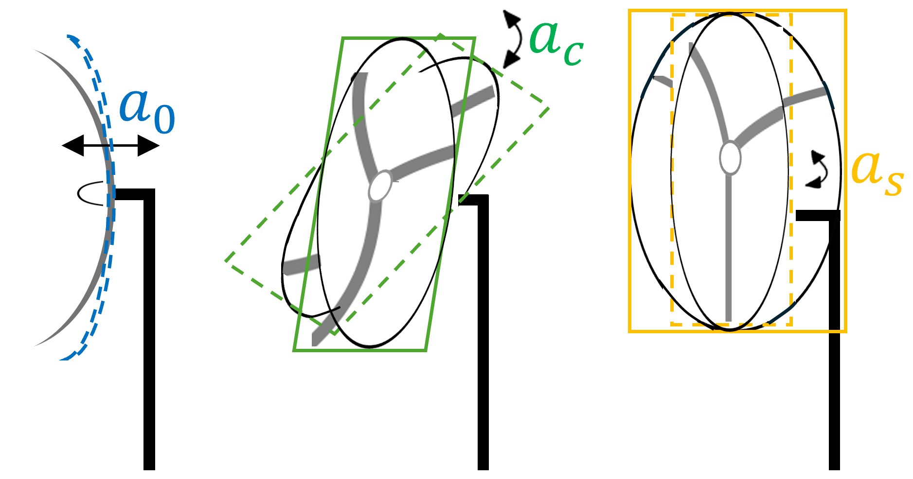
Figure 8 The three flap-wise motions of the blades expressed as non-rotational (NR) variables, which are the blade collective flap-wise (a₀), the rotor fore–aft tilting (a_c), and rotor yawing (a_s) motion amplitudes.

The Coleman matrix T⁻¹ transforms the four structural degrees of freedom from the rotational frame, $\mathit{x}={\left[{\mathit{\xi }}_{\mathrm{5}},a_{\mathrm{1}},a_{\mathrm{2}},a_{\mathrm{3}}\right]}^{\mathrm{T}}$, to the non-rotational one, ${\mathit{x}}_{\mathrm{NR}}={\left[{\mathit{\xi }}_{\mathrm{5}},a_{\mathrm{0}},a_c,a_{\mathrm{s}}\right]}^{\mathrm{T}}$, and its inverse T provides the opposite transform:

$$\begin{array}{}\text{(63)}& \begin{array}{rl}& \left[\begin{array}{c}{\mathit{\xi }}_{\mathrm{5}}\\ a_{\mathrm{0}}\left(t\right)\\ a_c\left(t\right)\\ a_{\mathrm{s}}\left(t\right)\end{array}\right]=\left[\begin{array}{cc}\mathrm{1}& \\ & \underset{{\mathbf{B}}_{\mathrm{3}\times \mathrm{3}}^{-\mathrm{1}}}{\underbrace{\left[\begin{array}{ccc}\mathrm{1}/\mathrm{3}& \mathrm{1}/\mathrm{3}& \mathrm{1}/\mathrm{3}\\ \mathrm{2}/\mathrm{3}\cos {\mathit{\psi }}_{\mathrm{1}}& \mathrm{2}/\mathrm{3}\cos {\mathit{\psi }}_{\mathrm{2}}& \mathrm{2}/\mathrm{3}\cos {\mathit{\psi }}_{\mathrm{3}}\\ \mathrm{2}/\mathrm{3}\sin {\mathit{\psi }}_{\mathrm{1}}& \mathrm{2}/\mathrm{3}\sin {\mathit{\psi }}_{\mathrm{2}}& \mathrm{2}/\mathrm{3}\sin {\mathit{\psi }}_{\mathrm{3}}\end{array}\right]}}\end{array}\right]\left[\begin{array}{c}{\mathit{\xi }}_{\mathrm{5}}\\ a_{\mathrm{1}}\left(t\right)\\ a_{\mathrm{2}}\left(t\right)\\ a_{\mathrm{3}}\left(t\right)\end{array}\right]\\ & \left[\begin{array}{c}{\mathit{\xi }}_{\mathrm{5}}\\ a_{\mathrm{1}}\left(t\right)\\ a_{\mathrm{2}}\left(t\right)\\ a_{\mathrm{3}}\left(t\right)\end{array}\right]=\left[\begin{array}{cc}\mathrm{1}& \\ & \underset{{\mathbf{B}}_{\mathrm{3}\times \mathrm{3}}}{\underbrace{\left[\begin{array}{ccc}\mathrm{1}& \cos {\mathit{\psi }}_{\mathrm{1}}& \sin {\mathit{\psi }}_{\mathrm{1}}\\ \mathrm{1}& \cos {\mathit{\psi }}_{\mathrm{2}}& \sin {\mathit{\psi }}_{\mathrm{2}}\\ \mathrm{1}& \cos {\mathit{\psi }}_{\mathrm{3}}& \sin {\mathit{\psi }}_{\mathrm{3}}\end{array}\right]}}\end{array}\right]\left[\begin{array}{c}{\mathit{\xi }}_{\mathrm{5}}\\ a_{\mathrm{0}}\left(t\right)\\ a_c\left(t\right)\\ a_{\mathrm{s}}\left(t\right)\end{array}\right].\end{array}\end{array}$$

Put differently, Eq. (63) translates to ${\mathit{x}}_{\mathrm{NR}}={\mathbf{T}}^{-\mathrm{1}}\mathit{x}$ and x=T x_NR. It means that we transform the original four structural degrees of freedom vector in the non-rotational basis by first excluding the three f_s,l aerodynamic variables associated with the dynamic stall model implementation. The equation of motion for the linear model from Eq. (26) is derived in the NR frame by multiplying both the left- and right-hand sides by T⁻¹ and by utilizing T and T⁻¹ to express the vector x and its time derivatives in the same frame:

$$\begin{array}{}\text{(64)}& \begin{array}{rl}& {\mathbf{T}}^{-\mathrm{1}}{\mathbf{M}}_S\underset{\ddot{\mathit{x}}}{\underbrace{\left(\ddot{\mathbf{T}}{\mathit{x}}_{\mathrm{NR}}+\mathrm{2}\dot{\mathbf{T}}{\dot{\mathit{x}}}_{\mathrm{NR}}+\mathbf{T}{\ddot{\mathit{x}}}_{\mathrm{NR}}\right)}}\\ & +{\mathbf{T}}^{-\mathrm{1}}\left({\mathbf{C}}_S+{\mathbf{C}}_A\right)\underset{\dot{\mathit{x}}}{\underbrace{\left(\dot{\mathbf{T}}{\mathit{x}}_{\mathrm{NR}}+\mathbf{T}{\dot{\mathit{x}}}_{\mathrm{NR}}\right)}}+{\mathbf{T}}^{-\mathrm{1}}{\mathbf{K}}_S\underset{\mathit{x}}{\underbrace{\left(\mathbf{T}{\mathit{x}}_{\mathrm{NR}}\right)}}\\ & =\underset{{\mathit{F}}_{L,\mathrm{NR}}}{\underbrace{{\mathbf{T}}^{-\mathrm{1}}{\mathit{F}}_L}}.\end{array}\end{array}$$

Here the forcing vector is set to be null due to the free vibration condition considered, i.e. ${\mathit{F}}_L={\mathit{F}}_{L,\mathrm{NR}}=\mathbf{0}$. From Eq. (64), the equation of motion in the non-rotational frame can be worked out by grouping together the matrix contributions that multiply individually the acceleration, velocity, and displacement vectors that are specified in the same frame too:

$$\begin{array}{}\text{(65)}& \begin{array}{rl}& \underset{{\mathbf{M}}_{\mathrm{NR}}}{\underbrace{\left({\mathbf{T}}^{-\mathrm{1}}{\mathbf{M}}_S\mathbf{T}\right)}}{\ddot{\mathit{x}}}_{\mathrm{NR}}+\underset{{\mathbf{C}}_{\mathrm{NR}}}{\underbrace{\left(\mathrm{2}{\mathbf{T}}^{-\mathrm{1}}{\mathbf{M}}_S\dot{\mathbf{T}}+{\mathbf{T}}^{-\mathrm{1}}\left({\mathbf{C}}_S+{\mathbf{C}}_A\right)\mathbf{T}\right)}}{\dot{\mathit{x}}}_{\mathrm{NR}}\\ & +\underset{{\mathbf{K}}_{\mathrm{NR}}}{\underbrace{\left({\mathbf{T}}^{-\mathrm{1}}{\mathbf{M}}_S\ddot{\mathbf{T}}+{\mathbf{T}}^{-\mathrm{1}}\left({\mathbf{C}}_S+{\mathbf{C}}_A\right)\dot{\mathbf{T}}+{\mathbf{T}}^{-\mathrm{1}}{\mathbf{K}}_S\mathbf{T}\right)}}{\mathit{x}}_{\mathrm{NR}}=\mathbf{0}.\end{array}\end{array}$$

All the components in Eq. (65), including the mass, stiffness, and damping matrices, are now represented as non-rotational variables. Thereafter, the contribution of the additional three aerodynamic DOFs f_s,l and the terms related to them need to be defined as non-rotational variables too and taken into account in the system matrix A_L,NR. The state vector q transformed in the NR frame is ${\mathit{q}}_{\mathrm{NR}}={\left[{\mathit{x}}_{\mathrm{4}\times \mathrm{1},\mathrm{NR}}^{\mathrm{T}},{\dot{\mathit{x}}}_{\mathrm{4}\times \mathrm{1},\mathrm{NR}}^{\mathrm{T}},f_{\mathrm{s},\mathrm{0}},f_{\mathrm{s},c},f_{\mathrm{s},s}\right]}^{\mathrm{T}}$, and it has a length of integer N_s. For instance, the system matrix ${\mathbf{A}}_{f_{\mathrm{s}}}$ is the first-order ODE Jacobian matrix for f_s, i.e. ${\mathbf{A}}_{f_{\mathrm{s}}}=\left[\partial {\dot{\mathit{f}}}_{\mathrm{s},i}/\partial {\mathit{f}}_{\mathrm{s},j}\right]$. The state-space ODE for the transformed state vector ${\mathit{q}}_{f_{\mathrm{s},\mathrm{NR}}}={\left[f_{\mathrm{s},\mathrm{0}},f_{\mathrm{s},c},f_{\mathrm{s},s}\right]}^{\mathrm{T}}$ is ${\dot{\mathit{q}}}_{f_{\mathrm{s},\mathrm{NR}}}={\mathbf{A}}_{\mathrm{fs},\mathrm{NR}}{\mathit{q}}_{f_{\mathrm{s},\mathrm{NR}}}$, and the matrix A_fs,NR is developed after some manipulations starting with the expression ${\mathit{q}}_{f_{\mathrm{s}}}=\mathbf{B}{\mathit{q}}_{f_{\mathrm{s},\mathrm{NR}}}$. The resulting system matrix A_L,NR is defined by the EOM that is described in the NR frame and by other transformed Jacobian matrices that are inserted,

$$\begin{array}{}\text{(66)}& \begin{array}{rl}& {\mathbf{A}}_{L,\mathrm{NR}}\\ & =\left[\begin{array}{ccc}\left[{\mathbf{0}}_{\mathrm{4}\times \mathrm{4}}\right]& \left[{\mathbf{I}}_{\mathrm{4}\times \mathrm{4}}\right]& \left[{\mathbf{0}}_{\mathrm{4}\times \mathrm{3}}\right]\\ \left[-{\mathbf{M}}_{\mathrm{NR}}^{-\mathrm{1}}{\mathbf{K}}_{\mathrm{NR}}\right]& \left[-{\mathbf{M}}_{\mathrm{NR}}^{-\mathrm{1}}{\mathbf{C}}_{\mathrm{NR}}\right]& \left[{\mathbf{M}}_{\mathrm{NR}}^{-\mathrm{1}}{\mathbf{T}}^{-\mathrm{1}}\left[\partial {\mathit{F}}_i/\partial {\mathit{f}}_{s,j}\right]\mathbf{B}\right]\\ \left[{\mathbf{B}}^{-\mathrm{1}}\left[\partial {\dot{\mathit{f}}}_{s,i}/\partial {\dot{\mathit{x}}}_j\right]\dot{\mathbf{T}}\right]& \left[{\mathbf{B}}^{-\mathrm{1}}\left[\partial {\dot{\mathit{f}}}_{s,i}/\partial {\dot{\mathit{x}}}_j\right]\mathbf{T}\right]& {\mathbf{A}}_{\mathrm{fs},\mathrm{NR}}\end{array}\right],\\ & {\mathbf{A}}_{\mathrm{fs},\mathrm{NR}}=\left[{\mathbf{B}}^{-\mathrm{1}}\left[\partial {\dot{\mathit{f}}}_{s,i}/\partial {\mathit{f}}_{s,j}\right]\mathbf{B}-{\mathbf{B}}^{-\mathrm{1}}\dot{\mathbf{B}}\right].\end{array}\end{array}$$

This system matrix A_L,NR is time-independent and can be used to calculate the eigenvalues without having to additionally rely on Hill's or Floquet's method to cancel out the periodicity of the system. This implies that the former periodicity of matrix A_L(t) has been eliminated.

The clear disadvantage of relying on the Coleman transform system is the complexity of the Coleman-transformed constant matrix A_L,NR compared to the time-varying counterpart A_L(t). Applying the Coleman transform to the parts of the matrix that define the coupling between the aerodynamic f_s,l states with the other structural states is not as trivial as obtaining the Coleman-transformed mass M_NR, damping C_NR, and stiffness K_NR constant matrices. Nevertheless, applying the Coleman transform is a computationally efficient approach if it renders the system LTI, because it is not expensive in comparison to other methods.

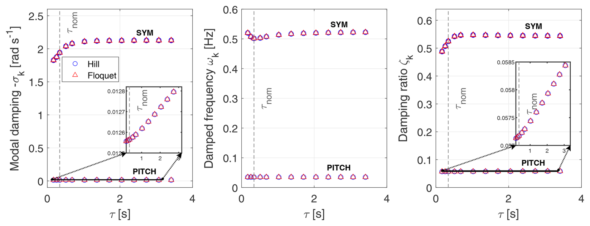
Figure 9 Modal damping, damped frequency, and damping ratio for an eigenvalue analysis in the rotational frame with a time constant τ variation.

7 Stability analysis

We now apply the stability methods on the linearized model to quantify the impact on the modal damping from the dynamic stall model's time constant τ and rotational speed Ω. Aerodynamic damping plays a major role in influencing the system's modal damping but also the damped frequency. The extent of that impact is thoroughly studied in this section.

Regarding the presentation of the stability analysis, the eigenvalues found in the rotational frame through Hill's and Floquet's methods are compared to the ones found in the non-rotational frame using the Coleman-transformed constant system matrix A_L,NR.

7.1 Time constant τ variation eigenvalue analysis

Our first stability study consists of analysing the evolution of eigenvalues while varying the time constant τ. We choose an operational point of V₀=8 m s⁻¹ and Ω=5.73 RPM. This is associated with the nominal time constant τ_nom=0.34 s. The steady state for that operational point is located in a specific region of the lift coefficient with respect to the angle of attack. That region is characterized by a flow which is partially attached and before C_L,static reaches a maximal value. In this particular study, the aerodynamic properties are all kept constant and only the time constant τ is varied without any influence on other variables, such as V_rel.

The eigenvalues that are associated with the dynamic stall aerodynamic DOFs f_s,l are omitted from plots. These eigenvalues are not physically relevant because the dynamic stall DOFs f_s,l only serve to express the aerodynamic damping of the system, and they can be correlated with a one-DOF dynamic system with a null frequency.

7.1.1 Rotational frame

Eigenvalues in Fig. 9 are expressed as a function of τ in the rotational frame for the floater pitch mode denoted by PITCH and for the symmetric blade mode denoted by SYM. Hill's (marked ∘) and Floquet's (marked △) results match, and they are presented in terms of modal damping σ_k, damped frequencies ω_k, and damping ratio ζ_k for these modes. This investigation serves to notice the impact of the eigenvalues with respect to the time constant and to observe after what time constant value and onward the blade damped frequencies, modal damping, and damping ratio have reached a plateau.

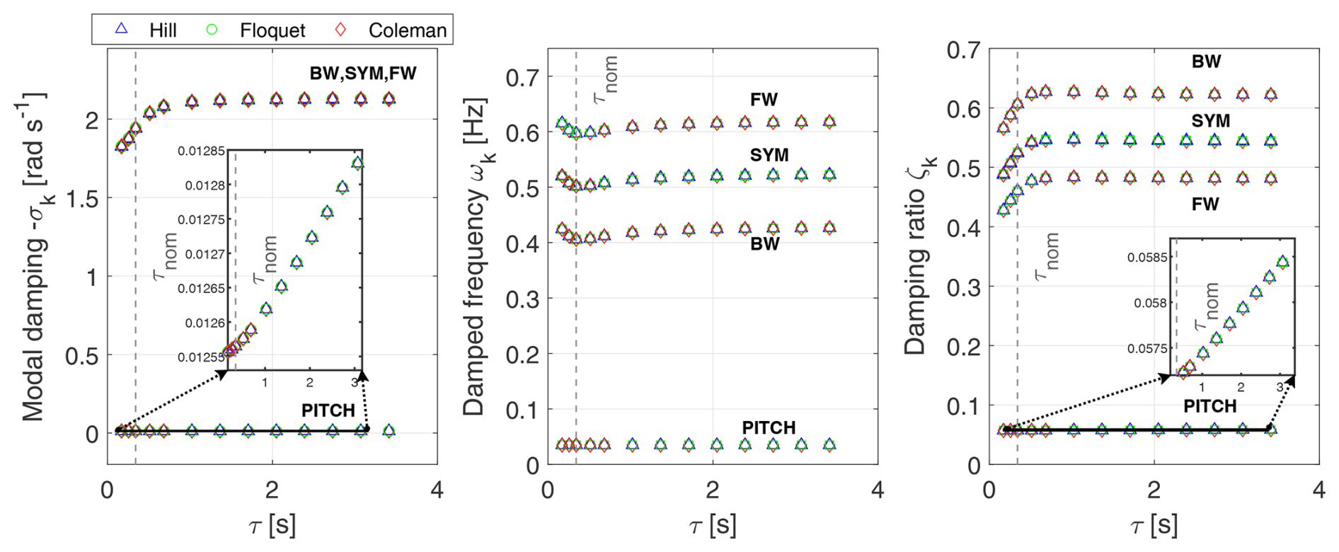
Figure 10 Modal damping, damped frequency, and damping ratio for an eigenvalue analysis in the NR frame with a time constant τ variation.

For the most part, the blade symmetric mode is not that affected by a larger time constant at values above the nominal one. The time constant does, however, slightly influence the growth of the floater pitch mode's modal damping and damping ratio. The damping ratio ζ_k is linked to the modal damping σ_k and to the principal damped frequency ω_p,k as follows:

$$\begin{array}{}\text{(67)}& {\mathit{\zeta }}_k={\displaystyle \frac{-{\mathit{\sigma }}_k}{\left|{\mathit{\omega }}_{p,k}\right|\sqrt{\mathrm{1}+\frac{{\mathit{\sigma }}_k^{\mathrm{2}}}{{\mathit{\omega }}_{p,k}^{\mathrm{2}}}}}}.\end{array}$$

When the modal damping σ_k is low in absolute value, evidently the damping ratio ζ_k can be approximated simply as the ratio of ${\mathit{\zeta }}_k\approx -{\mathit{\sigma }}_k/\left|{\mathit{\omega }}_k\right|$. The floater pitch damping ratio increases marginally with τ according to that approximation for ζ_k since its modal damping is very small while its damped frequency remains constant.

There is a strong correlation between the time constant τ and the dynamics of f_s,l (refer to Eq. 40) which in turn influences the dynamic stall lift coefficient C_L,l according to Eq. (28). This clarifies why the time constant τ has a noticeable effect on the blade modal damping, whereas it barely impacts the platform pitch modal damping. It can also be observed that the damped frequencies for the blade DOFs, a_l, get slightly larger with the time constant τ after the nominal value is surpassed. They increase until reaching a plateau value where τ's growth minimally affects the damped frequency and modal damping, since large values of τ lead to fixed values of f_s. Before the nominal τ value is reached, there is an augmentation of the blade DOFs' modal damping which leads to a reduction of the damped frequency. Concerning the damping ratio, it follows the same trend as the modal damping for both the symmetric blade mode and the floater pitch mode.

7.1.2 Non-rotational frame

Figure 10 shows in the non-rotational (NR) frame the modal damping σ_k, damped frequencies ω_k, and damping ratio ζ_k as a function of τ. Results are reported for Hill's (marked △), Floquet's (marked □), and Coleman's (marked ⋄) approach. In the frequency plot, the blade lowest damped frequency belongs to the rotor first backward-whirling (BW) mode, the middle damped frequency belongs to the first symmetric flap mode (SYM), and the highest damped frequency belongs to the first forward-whirling (FW) mode. The overall lowest damped frequency describes the floater pitch ξ₅ mode, and the lowest modal damping and damping ratio are also linked to that mode.

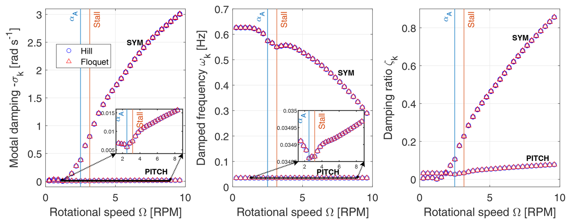
Figure 11 Modal damping, damped frequency, and damping ratio for a Campbell diagram eigenvalue analysis in the rotational frame with a rotational speed variation. The operational point is of V₀=8 m s⁻¹.

Results calculated via Hill's and Floquet's methods are originally found in the rotating frame, and they are reconstructed in the NR frame by applying the frequency shifts on the symmetric mode damped frequency to generate the rotor FW and BW modes. The rotor FW mode's damped frequency is shifted away from the rotor SYM mode's damped frequency by a constant distance of +Ω, and the rotor BW mode is shifted by −Ω where Ω=5.73 RPM = 0.0955 Hz is the rotational speed of the operational point. That being said, the modal damping is the same in both frames, implying that ${\mathit{\sigma }}_{k,\mathrm{NR}}={\mathit{\sigma }}_k$, while the damped frequency in the rotational frame is expressed in the NR frame through the following shifts:

$$\begin{array}{}\text{(68)}& {\displaystyle }{\mathit{\omega }}_{k,\mathrm{FW},\mathrm{NR}}={\mathit{\omega }}_{k,\mathrm{SYM}}+\mathrm{\Omega },{\mathit{\omega }}_{k,\mathrm{BW},\mathrm{NR}}={\mathit{\omega }}_{k,\mathrm{SYM}}-\mathrm{\Omega },\end{array}$$

given that ${\mathit{\omega }}_{k,\mathrm{SYM},\mathrm{NR}}={\mathit{\omega }}_{k,\mathrm{SYM}}$. Afterwards, the damping ratio ζ_k is found accordingly through Eq. (67) for all the blade modes,

$$\begin{array}{ll}{\displaystyle }{\mathit{\zeta }}_{k,\mathrm{FW},\mathrm{NR}}& {\displaystyle }={\displaystyle \frac{-{\mathit{\sigma }}_k}{\left|{\mathit{\omega }}_{k,\mathrm{FW},\mathrm{NR}}\right|\sqrt{\mathrm{1}+\frac{{\mathit{\sigma }}_k^{\mathrm{2}}}{{\mathit{\omega }}_{k,\mathrm{FW},\mathrm{NR}}^{\mathrm{2}}}}}},\\ \text{(69)}& {\displaystyle }{\mathit{\zeta }}_{k,\mathrm{BW},\mathrm{NR}}& {\displaystyle }={\displaystyle \frac{-{\mathit{\sigma }}_k}{\left|{\mathit{\omega }}_{k,\mathrm{BW},\mathrm{NR}}\right|\sqrt{\mathrm{1}+\frac{{\mathit{\sigma }}_k^{\mathrm{2}}}{{\mathit{\omega }}_{k,\mathrm{BW},\mathrm{NR}}^{\mathrm{2}}}}}},\end{array}$$

and ${\mathit{\zeta }}_{k,\mathrm{SYM},\mathrm{NR}}={\mathit{\zeta }}_{k,\mathrm{SYM}}$ applies again for the SYM mode. Once the eigenvalues determined with Floquet's and Hill's methods are transformed in the NR frame, they do perfectly match the ones calculated by directly solving the eigenvalue problem for the Coleman-transformed system matrix A_L,NR. As for the difference in damping ratio between the FW, SYM, and BW modes, it is due to the different damped frequencies for the three modes, because the modal damping is identical and not influenced by the frame considered. According to Eq. (67), because the modal damping is the same for all three rotor modes, a BW mode experiences a higher modal damping above the symmetric mode, whereas a FW mode experiences instead a lower damping ratio.

Since the rotational speed Ω is kept constant, the rotor BW, SYM, and FW modes' damped frequencies (distanced by 1×Ω from the SYM mode) and damping ratio values are equally spaced, and they remain unaffected by the time constant τ after the threshold of τ=1 s has been exceeded.

7.2 Rotational speed Ω variation – Campbell diagram

To validate once more the correct implementation of Hill's and Floquet's methods, an eigenvalue analysis for a varying rotational speed Ω is performed. The modal damping σ_k, damped frequency ω_k, and damping ratio ζ_k results are displayed on a Campbell diagram in the rotational and non-rotational frame. The operational point of V₀=8 m s⁻¹ and Ω=5.73 RPM is yet again located in the usual region before the maximal C_L,static is attained where the flow is partially attached. For this operational point, we compute the steady-state responses and the normal inflow velocity $V_{\widehat{n},l}$ which are kept constant for varying rotational speeds Ω. However, the rotational velocity is updated as $V_{\widehat{t},l}=-\mathrm{\Omega }d$, and the aerodynamic parameters are calculated accordingly with a varying angle of attack α. Using the eigenvalues calculated with Floquet's and Hill's method in the rotational frame, the rotor BW (−Ω) and FW (+Ω) modes are once again added on the damped frequency plot in the NR frame as offsets from the SYM blade mode. On the contrary, when solving the eigenvalues for the Coleman-transformed system, these modes manifest themselves because they are rotor modes associated with a global fixed coordinate system rather than being blade specific.

7.2.1 Rotational frame

The purpose of this stability analysis is to demonstrate that the stability methods can determine the aerodynamic damping as a function of rotational speed. An augmentation of the rotational speed Ω and of the tangential velocity component $V_{\widehat{t},l}$ amplifies the relative velocity V_rel,l while simultaneously decreasing the angle of attack α.

Results in Fig. 11 show that with a greater rotational speed Ω, the floater pitch motion's damped frequency does not rise significantly, but its modal damping increases slightly, causing the damping ratio to be amplified considerably. It is also seen in Fig. 11 that the damped frequency and modal damping predicted by Hill's (marked ∘) and Floquet's (marked △) methods are well matched.

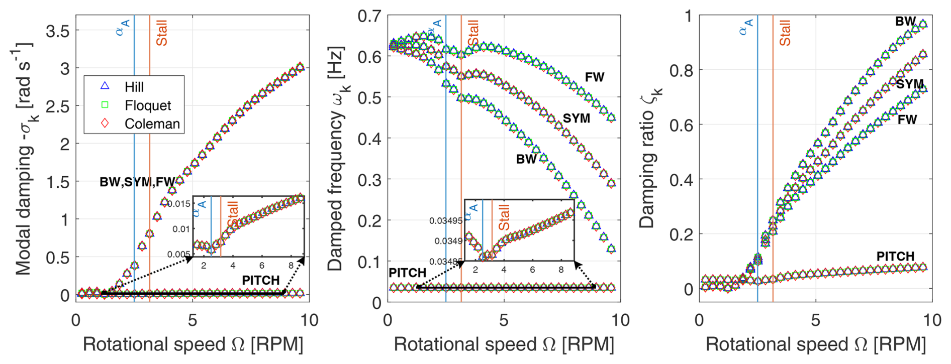
Figure 12 Modal damping, damped frequency, and damping ratio for a Campbell diagram eigenvalue analysis in the NR frame with a rotational speed variation. The operational point is of V₀=8 m s⁻¹.

Furthermore, the effect of increasing aerodynamic damping is observable notably in terms of a decreased blade DOF a_l damped frequency. The amplification of the relative velocity V_rel,l increases the aerodynamic damping through the lift loads and leads to a higher blade modal damping. Thus, at lower rotational speeds the symmetric blade mode has a very small modal damping and a low damping ratio too, which also applies to the floater pitch mode. At very low rotational speeds, the blade damping ratio is even smaller than the floater pitch one, but it grows drastically with rotational speed and overpasses it soon after. In view of this, with a higher aerodynamic damping at higher rotational speeds Ω, the damped frequency for the pitch DOF ξ₅ barely increases and remains almost unchanged in comparison to the apparent reduction of the blade damped frequencies. Nevertheless, the damping ratio also increases for the floater pitch mode in a linear way according to the approximation ${\mathit{\zeta }}_k\approx -{\mathit{\sigma }}_k/\left|{\mathit{\omega }}_k\right|$ that holds since its modal damping is very low, and the damped frequency remains almost unaffected. It ensues that the aerodynamic damping influences the eigenvalues of the blade DOFs more than the floater pitch eigenvalue.

The change in damped frequency at 3.16 RPM is due to the variation of C_L at that rotational speed with a corresponding angle of attack as can be seen in Fig. 4. At that particular angle of attack, the gradient $\partial f_{\mathrm{static},l}/\partial {\mathit{\alpha }}_l$ starts increasing locally. The resulting change in damped frequency at that RPM is caused by a high fluctuation of aerodynamic parameters, and it demonstrates that the stability analysis methods can detect the effect of stall parameter variations. Fluctuations at other rotational speeds are caused by gradual numerical changes too in the gradient $\partial f_{\mathrm{static},l}/\partial {\mathit{\alpha }}_l$ for corresponding angles of attacks as detailed in Fig. 4. The angle of attack noted α_A in Fig. 4 represents a sudden rise in the value of $\partial f_{\mathrm{static}}/\partial \mathit{\alpha }$ which disturbs mainly the floater pitch motion damping trend. That sudden change in $\partial f_{\mathrm{static},l}/\partial {\mathit{\alpha }}_l$ is connected to the stall region in Fig. 3, where the static lift coefficient starts decreasing with the angle of attack, while the full stall coefficient C_L,stall slope stops increasing. In short, the angle of attack region between the maximal C_L,static value (labelled Stall) and α_A is a region which impacts both the damping and damped frequency for the floater pitch motion and only the damped frequency for the blades.

7.2.2 Non-rotational frame

Comparing eigenvalues on a Campbell diagram with both Hill's (marked △) and Floquet's (marked □) method, as well as with the Coleman approach (marked ⋄), allows us to cross-validate them at last in the NR frame. Just like in Fig. 10 for the time constant τ variation eigenvalue analysis expressed in the NR frame, the rotor FW and BW modes are reconstructed as before from the SYM mode when using Hill's and Floquet's methods to compare with the Coleman-based results. The Campbell diagram in Fig. 12 proves that the eigenvalues found with either procedure are equal.

The three blade modes all have a modal damping that increases with rotational speed, while their damped frequencies decrease. To summarize, growth of modal damping and a drop of damped frequency simultaneously cause the damping ratio to rise with rotational speed. Moreover, for the NR frame, the blade DOF rotor FW mode is associated with a lower damping ratio curve, while the rotor BW mode is linked instead to a higher damping ratio curve. This occurs because all three blade modes are associated with the same modal damping; refer to the damping ratio expression in Eq. (67). The rotor's SYM mode curve is the middle one in both the damped frequency and damping ratio plots. The BW, SYM, and FW damped frequency and damping ratio curves become more distinguishable from each other at higher rotational speeds due to the application of the ±Ω frequency offset.

8 Two-bladed floating wind turbine model

The main motivation for developing the two-bladed floating wind turbine model is to test under different design circumstances and operational conditions the applicability of our developed Coleman-free aero-elastic stability methods, namely Hill's and Floquet's methods. As a reminder, using only the Coleman transform for a two-bladed rotor would not result in making the system LTI, which is another reason to rely on those methods in the first place. The Coleman transform for a two-bladed rotor does not use the azimuthal periodicity in its definition but rather its eigenmodes. For a two-bladed rotor, if one were to apply the Coleman transform, the periodicity of the system matrix could be eliminated through the use of a supplementary method such as Floquet's or Hill's method.

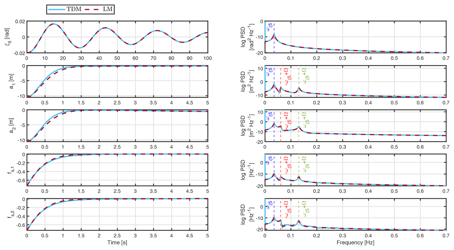
Figure 13 Decay test for the operational point of V₀=8 m s⁻¹, Ω=0.6 rad s⁻¹, and τ=0.512 s for the two-bladed wind turbine, where TDM and LM results are compared.

The two-bladed wind turbine model is obtained firstly by having a blade chord length c increased by a factor of $\mathrm{3}/\mathrm{2}$ compared to the three-bladed model (Kim et al., 2015). This chord length extension is applied for all airfoils across the whole blade length span. It accounts for the reduction of the number of blades so that the same lift, thrust, and torque were generated by both wind turbine models. This blade design change affects things equally, so the airfoil section of interest is at r=d. The two-bladed model EOMs differ from the three-bladed case due to the system matrix size reduction through an elimination of matrix rows and columns that pertain to the third blade components. In light of this, the structural DOF vector for the two-bladed wind turbine is ${\mathit{x}}_{\mathrm{3}\times \mathrm{1}}={\left[{\mathit{\xi }}_{\mathrm{5}},a_{\mathrm{1}},a_{\mathrm{2}}\right]}^{\mathrm{T}}$ in the EOM from Eq. (26). Subsequently, the state vector within the state-space ODE from Eq. (36) is $\mathit{q}={\left[{\mathit{x}}_{\mathrm{3}\times \mathrm{1}}^{\mathrm{T}},{\dot{\mathit{x}}}_{\mathrm{3}\times \mathrm{1}}^{\mathrm{T}},f_{\mathrm{s},\mathrm{1}},f_{\mathrm{s},\mathrm{2}}\right]}^{\mathrm{T}}$ and is of dimension N_s=8. The system matrices are thus fundamentally the same except for the scaling of the chord length and the matrix size reduction. The azimuthal angular Ψ_l position of the two blades is also changed as prescribed by Eq. (1) with N_b=2, and all system equations are modified accordingly.

8.1 Decay test

To verify that the two-bladed wind turbine linearized model has been rightfully built, decay test simulations are performed. Like for the three-bladed rotor case, results are presented in the time domain as variations from the steady states. The simulation time span is relatively short, because there is a focus on analysing the time responses of signals pertaining to the DOFs a_l and f_s,l until they reach their steady state. The simulation conditions that are considered are the same as for the three-bladed decay test in Fig. 5, meaning that an operational point of V₀=8 m s⁻¹ and Ω=0.6 rad s⁻¹ is applied. The resulting steady-state angle of attack and lift coefficient are still positioned in the same region before maximal C_L,static is obtained where the flow is partially attached. Once more, the structural DOF initial conditions for the simulation are the negative value of the steady-state values with corresponding dynamic stall f_s,l variable initial conditions, meaning that ${\mathit{\xi }}_{\mathrm{5}}(t=\mathrm{0})=-\mathrm{0.02}$ rad, $a_l(t=\mathrm{0})=-\mathrm{10.54}$ m, and $f_{\mathrm{s},l}(t=\mathrm{0})=-\mathrm{0.73}$.

Figure 13 presents the decay responses for the LM and TDM. We observe a slight difference in time series for the blade deflection amplitude a_l signals and for the dynamic stall variable f_s,l before reaching the steady state of the operational point. That difference in responses between the time domain and linear model originates from the initial conditions being considerably far away from the operational point's steady state. Nevertheless, it is clear that the linearized model generates consistent time responses compared to the time domain model.

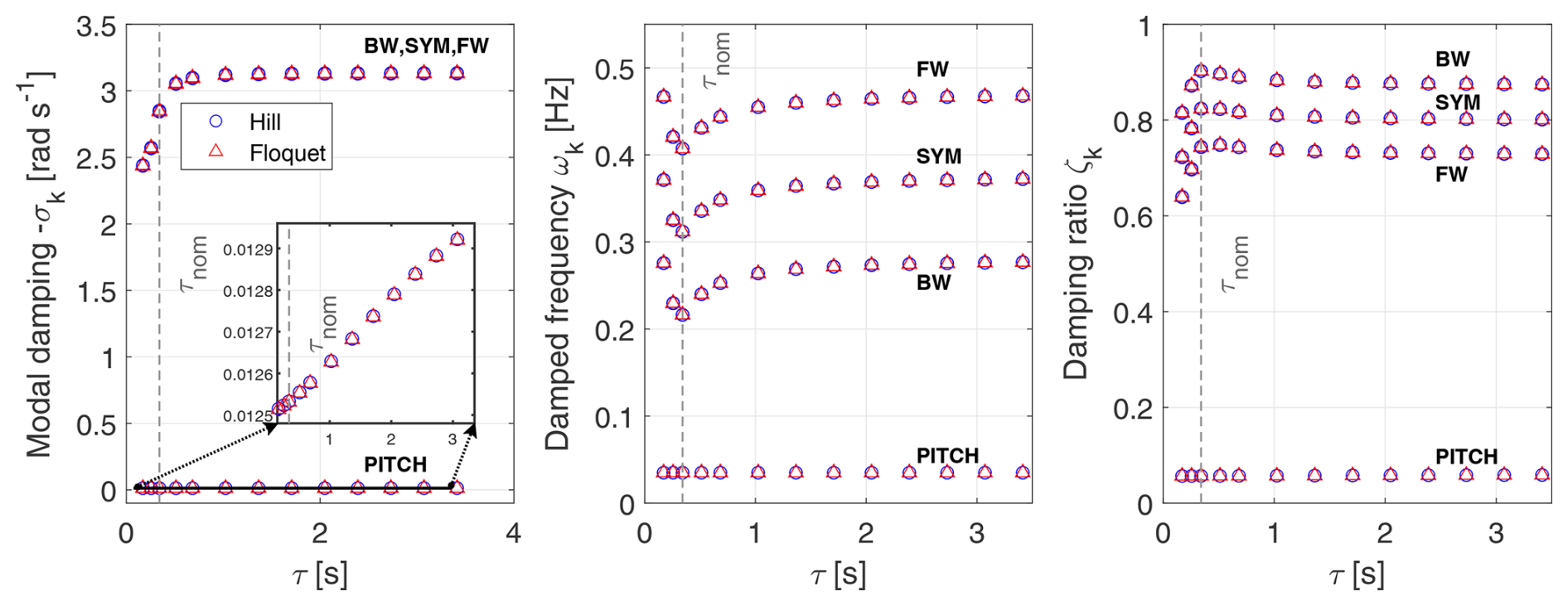
Figure 14 Modal damping, damped frequency, and damping ratio for an eigenvalue analysis in the NR frame with a time constant τ variation.

As anticipated, the time domain responses are converging fast towards the steady states also for the two-bladed model. Just like for the three-bladed wind turbine results from Fig. 5, the PSD plots do not capture the blade DOF a_l natural frequency, ω_1f=0.6255 Hz, because the aerodynamic damping effect prevents it. However, the natural frequency of the floater pitch motion, ${\mathit{\omega }}_{{\mathit{\xi }}_{\mathrm{5}}}$, is clearly observable as a peak value in the ξ₅ signal, and other natural frequencies of the system are not observable in this signal due to its own natural frequency dominant effect. Similarly to results for a three-bladed rotor in Fig. 5, the other signals for the a_l and f_s,l DOFs also show peaks at the frequencies of $-{\mathit{\omega }}_{{\mathit{\xi }}_{\mathrm{5}}}+\mathrm{\Omega }$ and ${\mathit{\omega }}_{{\mathit{\xi }}_{\mathrm{5}}}+\mathrm{\Omega }$, which are caused by the system's periodicity.

8.2 Eigenvalue analysis

For the eigenvalue analysis of the two-bladed wind turbine, the applicability of Floquet's and Hill's method remains to be demonstrated by executing the same studies as previously done for the three-bladed rotor. It is also relevant to analyse the distinctions in the eigenvalue trends between those computed for the two- and three-bladed rotor. This is relevant in particular for the Campbell diagram study.

The eigenvalues are originally computed in the rotational frame because the Coleman transform is not applicable for the two-bladed rotor. Despite that, they are expressed in the NR frame through a reconstruction of the rotor BW and FW modes.

8.2.1 Time constant τ variation eigenvalue analysis

With regard to the eigenvalue analysis for a varying time constant τ, results for the two-bladed wind turbine in Fig. 14 are similar to the three-bladed case in terms of tendency to reach plateau values with an increasing τ. The current eigenvalue results consider the same simulation conditions as for the three-bladed rotor simulations in the same region, meaning that the operational point still has an inflow velocity of V₀=8 m s⁻¹, and a rotational speed of Ω=5.73 RPM, but a nominal time constant of τ_nom=0.512 s instead. Similarly to previous results in Fig. 9 for the three-bladed rotor, the blade damped frequency is smallest at the nominal τ value for the current operational point. Furthermore, for the rotor BW and FW modes, the blade damped frequencies are shifted again by a constant rotational speed Ω=5.73 RPM away from the SYM blade mode's damped frequency. In accordance with previous results, the floater pitch damped frequency remains almost constant, whereas its modal damping σ increases proportionally to τ and consequently so does its damping ratio ζ. The only distinction between the two- and three-bladed rotor results in Figs. 14 and 10 is the modal damping and damped frequency 16values magnitude for the blade DOFs. For the two-bladed rotor, the blade damped frequencies are lower, while the modal damping and damping ratio are considerably higher. Due to its increased chord length, the two-bladed rotor experiences higher aerodynamic loads on each blade and, for that reason, a higher aerodynamic damping.

8.2.2 Rotational speed Ω variation – Campbell diagram

On the subject of eigenvalue results for the Campbell diagram study, the two-bladed rotor's BW and FW modes can only be obtained through the frequency shift away from the blade symmetric mode since the Coleman transform is not applicable in this context. Figures 15 and 16 report the Campbell diagrams for two operational points with the same rotational speed of Ω=5.73 RPM that are located in the region before C_L,static is maximal for a partially attached flow. Their inflow velocities are, respectively, V₀=8 m s⁻¹ and 10 m s⁻¹, and their corresponding nominal time constants are τ_nom=0.512 s and τ_nom=0.508 s. The operational point is used to get the steady states and the normal inflow velocity $V_{\widehat{n},l}$ but not the rotational velocity which is updated as $V_{\widehat{t},l}$ with −Ωd as well as the time constant τ, accordingly. We consider here these two different inflow velocities when investigating the eigenvalue trends to support our conclusions on the matter for the three- and two-bladed rotor design.

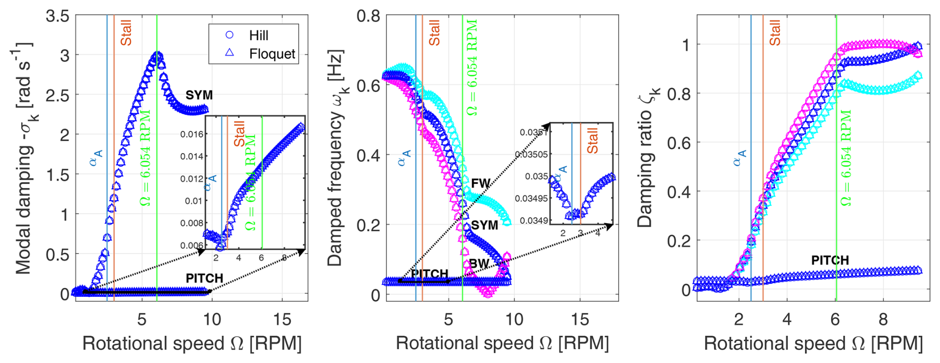
Figure 15 Modal damping, damped frequency, and damping ratio for a Campbell diagram eigenvalue analysis in the NR frame with a rotational speed variation. The operational point is of V₀=8 m s⁻¹.

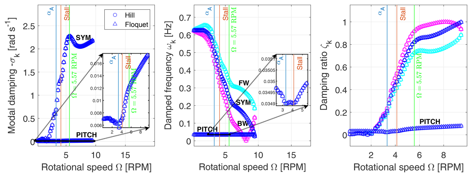
Figure 16 Modal damping, damped frequency, and damping ratio for a Campbell diagram eigenvalue analysis in the NR frame with a rotational speed variation. The operational point is of V₀=10 m s⁻¹.

First, in Figs. 15 and 16, the occurrence of maximal C_L,static around 3.00 RPM for an inflow velocity of V₀=8 m s⁻¹ and 4.1216 RPM for V₀=10 m s⁻¹ has a noticeable influence on the damped frequencies of the blades, which is similar to what was detected in Fig. 11 for the three-bladed rotor. As noted earlier for the three-bladed rotor, according to the variation of $\partial f_{\mathrm{s},\mathrm{static}}/\partial \mathit{\alpha }$ in Fig. 4 with respect to the angle of attack, there is a high impact on the analysis of the eigenvalues in the region of proximity of maximal C_L,static, between the angle of attack labelled “Stall” and the angle of attack α_A. Likewise, it can be observed in Figs. 15 and 16 that the two-bladed rotor's floater pitch motion's damped frequency and especially its damping are highly fluctuating in that angle of attack region. The blade damped frequencies are also highly impacted by the local variation of aerodynamic parameters in that region.

For the results with an inflow velocity of V₀=8 m s⁻¹ compared to V₀=10 m s⁻¹, an overall higher blade modal damping is observed, because the angles of attack are lower for the same rotational speeds in the angle of attack region before maximal C_L,static is reached, meaning below 15 deg. According to the airfoil data in Fig. 3, in that region lower angles of attack are associated with a greater f_s value and with a lower C_L,inv, but the C_L,stall value can vary. Thus, the overall value of the dynamic lift coefficient C_L can increase due to the impact of the dynamic stall variable f_s; refer to Eq. (28). A higher lift coefficient C_L would increase the lift force and ultimately generate a higher blade modal damping. Conversely, in the region where the flow is partially attached and near the maximal value of C_L,static, a higher angle of attack value generates greater C_L,inv and C_L,stall. This comes along with a lower f_s which can also increase the overall value of the dynamic lift coefficient C_L, depending on the impact of the dynamic stall variable f_s.

As a marked difference from the three-bladed rotor, a pronounced maximum in the blade modal damping is reached for a rotational speed of 6.054 RPM for V₀=8 m s⁻¹ and 5.57 RPM for V₀=10 m s⁻¹. The higher modal damping occurs for the lower inflow velocity of V₀=8 m s⁻¹, where the modal damping increases with rotational speed until reaching a maximal value at a lower angle of attack around α=7.78 deg compared to α=11.52 deg for the higher inflow velocity of V₀=10 m s⁻¹. At that particular rotational speed, the angle of attack is positioned before it is attained. The blade modal damping and damped frequency curves for V₀=10 m s⁻¹ fluctuate more because of a higher lift load variation with a greater inflow velocity. In this context, the two-bladed rotor experiences higher aerodynamic loads through higher lift loads because of the chord length being increased. Therefore, a small variation of the angle of attack, particularly at higher inflow velocities V₀ with greater lift variations, can cause such fluctuations in the eigenvalues. This difference in modal behaviour on a Campbell diagram is a characteristic of the two-bladed floating wind turbine that is accentuated compared to the three-bladed rotor.

Moreover, the attained maxima of blade modal damping are different compared to the three-bladed case. For example, as mentioned previously, at V₀=8 m s⁻¹ the blade modal damping maxima occur at Ω=6.054 RPM. We investigate this further in Fig. 17 when a change in trend with rotational speed Ω occurs for the gradient $\partial {\dot{\mathit{f}}}_{\mathrm{s},i}/\partial {\dot{\mathit{x}}}_j$, which is the partial derivative of the dynamic stall variable f_s with respect to the structural DOFs time-derived vector $\dot{\mathit{x}}$. The overall variation of the gradient $\partial {\dot{\mathit{f}}}_{\mathrm{s},i}/\partial {\dot{\mathit{x}}}_j$ components in the LTI system matrix is evaluated as a 1-norm ($\left|\right|\cdot |{|}^{\mathrm{1}}$), which is a sum of matrix components in absolute value. Results for $\partial {\dot{\mathit{f}}}_{\mathrm{s},i}/\partial {\dot{\mathit{x}}}_j$ are investigated using Hill's matrix A_L,0, i.e. $\left|\right|\mathrm{\Sigma }{\dot{\mathit{f}}}_{\mathrm{s},i}/\partial {\dot{\mathit{x}}}_j|{|}_{{\mathbf{A}}_{\mathrm{0}}}^{\mathrm{1}}$, and using Floquet's diagonalized matrix with updated eigenvalues and corresponding damped frequency shifts $\widehat{\mathbf{R}}$, i.e. $\left|\right|\mathrm{\Sigma }{\dot{\mathit{f}}}_{\mathrm{s},i}/\partial {\dot{\mathit{x}}}_j|{|}_{\widehat{\mathbf{R}}}^{\mathrm{1}}$. We also investigate eigenvector changes with rotational speed Ω to understand the causes for the variation of blade modal damping. Upon inspection of the structural mode eigenvectors $\mathit{v}=[v_{\mathrm{1}},\mathrm{\dots },v_{\mathrm{8}}{]}^{\mathrm{T}}$, we identify the symmetric blade mode eigenvector v_SYM as having only blade amplitude components a_l for the displacement (v_SYM,2 and v_SYM,3) and velocity (v_SYM,5 and v_SYM,6) DOFs, as well as dynamic stall values for the f_s,l DOFs (v_SYM,7 and v_SYM,8). When considering the absolute value of eigenvectors, $\left|\mathit{v}\right|$, with respect to their real and imaginary parts, we notice for the symmetric blade mode that only the f_s,l components, which are equal ($\left|v_{\mathrm{SYM},\mathrm{7}}\right|=\left|v_{\mathrm{SYM},\mathrm{8}}\right|$), vary with rotational speed Ω. The same trend as for the gradient $\partial {\dot{\mathit{f}}}_{\mathrm{s},i}/\partial {\dot{\mathit{x}}}_j$ is observed at the rotational speed of maximal blade modal damping for the SYM blade mode's eigenvector dynamic stall components evaluated as absolute values, $\left|v_{\mathrm{SYM},\mathrm{7}}\right|=\left|v_{\mathrm{SYM},\mathrm{8}}\right|=\left|{\mathrm{v}}_{\mathrm{SYM},f_{\mathrm{s},l}}\right|$. This points out the high correlation in this case between the gradient $\partial {\dot{\mathit{f}}}_{\mathrm{s},i}/\partial {\dot{\mathit{x}}}_j$ and the SYM blade mode. Onward from the rotational speed of maximal blade modal damping, there is a visible change in shape for the resulting curves. For V₀=10 m s⁻¹, these changes occur at Ω=5.57 RPM, according to Fig. 18. We also observe in Figs. 17 and 18 that the curves for the gradient $\partial {\dot{\mathit{f}}}_{\mathrm{s},i}/\partial {\dot{\mathit{x}}}_j$ and for the symmetric mode eigenvector dynamic stall variable reach a maximal value at a rotational speed associated with the angle of attack in the region where C_L,static is maximal. All these observations indicate that for varying rotational speeds the dynamic stall gradient $\partial {\dot{\mathit{f}}}_{\mathrm{s},i}/\partial {\dot{\mathit{x}}}_j$ relates to the SYM blade mode and consequently the blade modal damping.

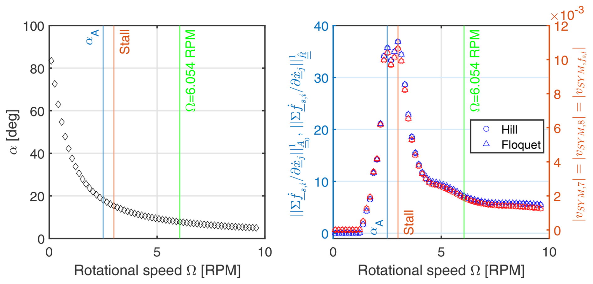
Figure 17 Angle of attack α, 1-norm of the gradient $\partial {\dot{\mathit{f}}}_{\mathrm{s},i}/\partial {\dot{\mathit{x}}}_j$ components, and dynamic stall component of the symmetric blade mode ($\left|{\mathrm{v}}_{\mathrm{SYM},f_{\mathrm{s},l}}\right|$) for the LTI system matrix using Hill's and Floquet's methods. The rotational speed Ω is varied for the operational point of V₀=8 m s⁻¹.

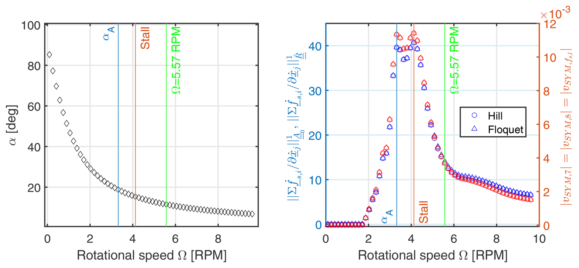
Figure 18 Angle of attack α, 1-norm of the gradient $\partial {\dot{\mathit{f}}}_{\mathrm{s},i}/\partial {\dot{\mathit{x}}}_j$ components, and dynamic stall component of the symmetric blade mode ($\left|{\mathrm{v}}_{\mathrm{SYM},f_{\mathrm{s},l}}\right|$) for the LTI system matrix using Hill's and Floquet's methods. The rotational speed Ω is varied for the operational point of V₀=10 m s⁻¹.

Finally, for the two-bladed rotor, an increased chord length gives overall a larger lift and a larger blade modal damping. At large RPM values, the blade damping is so strong (ζ≈1) that the damped frequency tends to zero. As a consequence, it can be seen for both test cases in Figs. 15 and 16 that the rotor backward-whirling mode reaches a critical damping state when the damping ratio is ζ=1. The rotor backward-whirling mode also experiences a reflection of its damped frequency once reaching a null value, because a negative frequency is not physically plausible.

9 Conclusions

A three-bladed floating wind turbine time domain model and a linear model were established to devise Coleman-free methods for aero-elastic stability analysis. It was demonstrated how the presence of gravity leads to additional terms in the stiffness matrix that couples the blade deflection and floater pitch, thus introducing a dependency to the floater equilibrium tilt angle for the stability analysis. This tilt dependency on the structural dynamics disappeared when gravity was excluded. The aerodynamic states were included in the model through the dynamic stall variable f_s with its respective ODE, and then the time domain model was linearized with the inclusion of the aerodynamic damping contribution. The time domain and linear models enabled us to do a first dynamic stall analysis by varying the floater pitch excitation intensity for different operational points where stall occurs, which verified the match between the two models. Another time domain hysteresis analysis was conducted with the time constant τ being fixed at different values while operating in the partially attached flow region before the static lift coefficient C_L,static is maximal. Those analyses verified that both the time domain and linear models were consistent and that they represented the wished for physical behaviour of the floating wind turbine.

Afterwards, the three-bladed linear model was rendered time-independent through the use of Hill's and Floquet's methods. Once the linear model was made time-invariant, all stability analyses proved that the impact of aerodynamic states is observable in terms of both modal damping and damped frequency. For the sake of completeness and understanding of Hill's and Floquet's methods, the eigenvalue results were cross-validated with each other for multiple stability studies. The first eigenvalue analysis was carried out for a varying time constant τ, and it demonstrated that both methods produced matching results that included the damping influence of the aerodynamic states. The next eigenvalue analysis was accomplished on a Campbell diagram where the rotational speed was varied. Results showed again perfect agreement between the eigenvalues provided by both methods. Following those eigenvalue studies, a modification of the frame, from a rotating frame to a fixed non-rotating one, was applied to the system through the Coleman transform. The evolution of eigenvalues with respect to the variation of τ and rotational speed Ω was examined in the new frame too. These results were compared to previous ones expressed in the rotating frame, and they were identical irrespective of the method applied, Floquet's or Hill's. This comparison illustrated that having stability analyses executed for a Coleman-free system provides the same eigenvalues for the blade symmetric mode as with the Coleman-transformed system. Using Hill's and Floquet's eigenvalues computed in the rotational frame, it was proven that it is possible to reconstruct the rotor forward- and backward-whirling mode eigenvalues of the model so that they are identical to those obtained directly with the Coleman-transformed system matrix.

Finally, a two-bladed rotor model was implemented for the main objective of investigating the change in eigenvalues in a Campbell diagram compared to results for the three-bladed rotor model. Two different inflow velocity cases were tested. The same Hill and Floquet methods were applied for the two-bladed stability studies, and both of them produced matching results again. Both methods were utilized for the two-bladed rotor too to reconstruct the rotor forward- and backward-whirling modes with the frequency shift of ±Ω away from the symmetric blade mode. Results have shed light on the major differences that can be present for the two-bladed wind turbine stability analysis. Just like for the three-bladed rotor, the region where C_L,static is maximal had a noticeable impact on the two-bladed rotor's eigenvalues. The blade modal damping had a distinct peak at the rotational speed of Ω=6.054 RPM for an inflow velocity of V₀=8 m s⁻¹, whereas the peak was located at Ω=5.57 RPM for an inflow velocity of V₀=10 m s⁻¹. This observation was investigated further through inspection of the dynamic stall gradient of $\partial {\dot{\mathit{f}}}_{\mathrm{s},i}/\partial {\dot{\mathit{x}}}_j$ with respect to the structural DOF velocity vector $\dot{\mathit{x}}$. The 1-norm value of the gradient $\partial {\dot{\mathit{f}}}_{\mathrm{s},i}/\partial {\dot{\mathit{x}}}_j$ components (summed absolute values) was considered for the LTI system matrix with Hill's (matrix A_L,0) and Floquet's methods (updated diagonalization matrix $\widehat{\mathbf{R}}$). It was observed that the maximum blade modal damping was seen to coincide with a change of curve trend for the stall gradient as well as for the symmetric blade mode's dynamic stall DOF f_s. For varying rotational speeds Ω (and angles of attack α), the change caused by the gradient $\partial {\dot{\mathit{f}}}_{\mathrm{s},i}/\partial {\dot{\mathit{x}}}_j$ in the system matrix generated a fluctuation with the same trend observed in the symmetric blade mode's eigenvector dynamic stall variable f_s value.

In line with previous studies, special attention was needed for the selection of the principal damped frequencies when applying both Hill's and Floquet's methods. When using Hill's method, the principal damped frequency selection was facilitated because the Frobenius norm of the zeroth harmonic matrix A_L,0 from the Fourier expansion of A_L(t) was much larger than for higher harmonic matrices; refer to Eq. (51). This means that the truncation of $\widehat{\mathbf{A}}$ could be done while still preserving the accuracy of its eigensolutions. One could select the principal damped frequencies as being closest to the ones associated with A_L,0. The drawback of Floquet's method was that it was computationally demanding in time duration compared to Hill's method. Essentially, it was a numerically less efficient method on account of the need to compute the transition state or monodromy matrix by carrying out as many decay simulations of a period duration as there are states. However, for situations where the system matrix is not available or for the analysis of experimentally acquired time series, Floquet's method would be a better alternative compared to Hill's method. In that case, the monodromy matrix could be extracted directly from responses after a period without further need for simulation. Although Hill's method relied on a bigger expanded state-space matrix to solve the eigenvalue problem, it was still computationally less costly than Floquet's method in our context. In spite of that, we found that both methods are reliable and accurate to provide consistent and identical eigenvalue results.

In summary, Hill's and Floquet's methods can be used for any linear state-space model and thus in principle also for linearized versions of aero-elastic models. We have demonstrated their functionality here on a simple model with floater pitch and aerodynamic states. If we were to include not only the blade deflection contributions from the first flap-wise (1f) but also the second flap-wise (2f) and first edge-wise (1e) modes, there would be the corresponding blade deflection amplitude DOFs a_1f,l, a_2f,l, and a_1e,l in the model with the velocity triangle updated and partial derivatives calculated with respect to the time derivatives of those DOFs. However, the number of aerodynamic states would remain unchanged. Similarly to the modal superposition method used for computing the blade deflections, the same can be done if considering the tower deflections by adding the tower mode deflection amplitudes as additional DOFs and updating too, accordingly, the partial derivatives and velocity triangle.

Future work will focus on relying on Hill's method for fast response calculations by using improved approaches compared to our previous methodology (Pamfil et al., 2024).