Analysis and calibration of optimal power balance rotor-effective wind speed estimation schemes for large-scale wind turbines

The size growth of modern wind turbines creates challenges in their control system design, particularly due to greater wind variability across larger rotor areas. As modern turbine control systems rely on the availability of accurate wind speed information, the increasing unrepresentativeness of pointwise measurement devices, such as anemometers, necessitates the incorporation of more representative rotor-effective wind speed (REWS) estimation. Classical REWS estimators, based on static power relations, often fail to account for dynamic changes, leading to inaccurate estimation. To overcome these challenges, this paper introduces a power-balance-based REWS estimation framework and splits the estimation problem into two modules: an aerodynamic power estimator and a wind speed estimate solver. Two possible aerodynamic power estimation techniques are discussed based on numerical derivative and state estimation. As state estimator calibration remained a challenge for varying wind turbine sizes, a gain-tailoring method for the performance calibration throughout a range of modern wind turbine sizes has been derived for the state-estimation-based aerodynamic power estimator. Two types of wind speed estimate solvers are analyzed, namely the continuous and iterative single-step methods. From the two modules, the best-performing methods – the state estimation aerodynamic power estimator and iterative single-step wind speed solver – are chosen to form the optimal power balance REWS estimator. The combined optimal estimator is validated through OpenFAST simulations of the National Renewable Energy Laboratory (NREL) 5 MW and IEA 22 MW turbines and compared against a baseline method. The proposed method demonstrates good tracking of the REWS, better noise resilience, and convenient estimator gain calibration across different turbine sizes.

1 Introduction

With the increasing demand for clean and renewable wind energy for the provision of electricity worldwide, there is a trend toward upscaling wind turbine sizes (Global Wind Energy Council, 2024). Greater wind turbine rotor-swept areas enable more wind energy to be harnessable, resulting in increasing power production per unit turbine and effectively lowering the so-called levelized cost of energy – thus making wind turbines more competitive in the energy market (Burton et al., 2011; Veers et al., 2019).

Regardless of the potential economic benefit, the task of controlling wind turbines with larger rotors is becoming more of a challenge, especially when accurate information on wind speed is crucial to ensure high controller performance, e.g., for gain scheduling (Kumar and Stol, 2009; Koerber and King, 2013), feedforward (feedback) control (Van Engelen and Van der Hooft, 2003; Koerber and King, 2013; Lazzerini et al., 2024), or tip-speed ratio tracking (Bossanyi, 2000; Ortega et al., 2013; Abbas et al., 2022; Brandetti et al., 2022, 2023), to mention a few. This is mainly caused by the greater spatial variability across the rotor-swept area for larger turbines. Thus, pointwise wind speed information, such as that provided by anemometers downstream at the nacelle, becomes increasingly unrepresentative, not to mention the presence of highly perturbed wind flow at the rotating turbine blades (Soltani et al., 2013). On the other hand, being the main driving force of a wind turbine, the deduction of more representative wind speed information via the turbine dynamics has been seen as a viable alternative (Boukhezzar and Siguerdidjane, 2011). To be more exact, other available measurements, namely rotor speed, generator torque signal, and blade pitch position, can be used to provide the so-called rotor-effective wind speed (REWS) estimate (Østergaard et al., 2007).

Early REWS estimation studies (see Østergaard et al., 2007; Soltani et al., 2013, and references therein), in large part, utilize the static relation between the produced power and the REWS by omitting the always-occurring dynamical changes in the rotor speed. Resultingly, these REWS estimators cannot provide accurate estimations of the aerodynamic torque in transient conditions due to the neglected dynamic information.

To address the aforementioned shortcoming, later REWS estimation studies incorporating rotor acceleration information in their framework arose in the literature. In Bossanyi (2000), the REWS estimate is obtained by first estimating the aerodynamic torque by reformulating torque balance drivetrain dynamics, which account for rotor acceleration and drivetrain inertial information. Then, given a priori knowledge of the aerodynamic torque coefficient table, it is possible to deduce the information on the wind speed.¹ The work of Van Engelen and Van der Hooft (2003) and Boukhezzar and Siguerdidjane (2011) adopts a similar estimation approach, where for the wind speed estimate solver, the Newton–Raphson algorithm, being an iterative single-(time)step method, is utilized. In Ortega et al. (2013), an immersion and invariance method for the wind speed estimation is employed, and its global convergence guarantee is provided. This method seeks to nullify the error between measured rotor speed and its estimate, with the latter being the integrated difference between the (inertia-scaled) generator torque and the aerodynamic torque estimate, using a proportional compensator (and an integrator, as extended by Liu et al., 2022). Having canceled the rotor speed estimation error, the wind speed estimate is then obtained in a continuous manner. The continuous method, in comparison with the iterative method, is considered to be a multiple-time-step solving scheme.

Nevertheless, stability analysis of the continuous solver following a discretization has remained unaddressed, to the best of the authors' knowledge. Moreover, the performance comparison between the two wind speed estimation solving methods has received little attention in the literature.

With regard to the aerodynamic torque (or power estimator), the work of Østergaard et al. (2007) is of particular interest. Two ways to obtain the aerodynamic torque estimate are studied therein, namely (filtered) numerical derivative and state estimation. The former is associated with the numerical differentiating method used to obtain the rotor acceleration estimate from measured rotor speed. This provides a necessary “ingredient” to reconstruct aerodynamic torque given a priori inertia information and generator torque input. The latter method provides two cascaded observers. The inner loop estimates the unmeasurable turbine states by Kalman filtering, while the outer one estimates the aerodynamic torque by a proportional–integral compensator structure. Although performance comparisons of both methods are provided, little attention was paid to the effect of noisy measurements on the aerodynamic torque estimators, which might deteriorate the ensuing wind speed estimation. To facilitate calibration of wind speed estimation by state estimation, the work of Moustakis et al. (2019) proposed a machine-learning-based Bayesian optimization approach. Nonetheless, since it remained unclear how to properly tune such a wind speed estimator, a Bayesian optimization approach, which is a global optimization machine learning algorithm, was adopted in the study.

However, optimal wind speed estimator tuning for a single turbine might not necessarily translate into optimal performance when applied to a different turbine. Given the accelerated growth in modern wind turbine sizes, there is a need for deriving a calibration methodology to ensure optimal estimator tuning throughout these turbines.

Furthermore, based on the above literature review, four possible combinations of the aerodynamic torque (or aerodynamic power, as made clearer shortly) estimator and wind speed estimate solver can be constructed with the optimal combination left undetermined. Moreover, validation in realistic simulation settings of such an optimal wind speed estimator combination – calibrated for wind turbines of various sizes – needs to be performed. It is also worth noting that the aforementioned works on various wind speed estimator schemes are based on the torque balance modeling of the wind turbine drivetrain. While such torque-based coordinates have been widely used for wind turbine control designs in the literature, employing power-based terms to represent wind turbine dynamics is common practice in industry (Hovgaard et al., 2015; Odgaard et al., 2017; Brandetti et al., 2022; Mulders et al., 2023a; Pamososuryo et al., 2023). The current work thus provides a wind speed estimator framework largely based on power balance dynamics. Nevertheless, adopting this work into the torque balance framework is straightforward. The contributions of this work are outlined as follows:

1. A thorough analysis for numerical-derivative- and state-estimation-based aerodynamic power estimators in noisy measurement settings is provided.

2. A calibration methodology for a state-estimation-based aerodynamic power estimator for a range of modern wind turbine sizes is formulated.

3. Iterative and continuous wind speed estimate solvers are derived, and frequency-domain stability analysis for the latter-mentioned method is provided.

4. The optimal wind speed estimator structure is identified from the proposed aerodynamic power estimators and wind speed estimate solvers.

5. A mid-fidelity validation of the selected optimal estimator under realistic conditions for multiple wind turbine sizes is provided.

The remainder of this paper is structured as follows: in Sect. 2, preliminaries required for this paper, being the notation convention, key reference wind turbine properties, and assumptions used throughout the paper, are explained. Section 3 touches upon the closed-loop wind turbine model and the proposed power balance REWS estimation framework. Sections 4 and 5 address several potential options for the aerodynamic power estimator and wind speed estimate solver subcomponents, respectively, where thorough analyses and low-fidelity numerical demonstrations are given. In Sect. 6, the proposed combinations of the aerodynamic power estimator and wind speed estimate solver subcomponents are validated using higher-fidelity wind turbine simulation results. Finally, the conclusions and recommendations of this work are laid out in Sect. 7.

2 Preliminaries

2.1 Notations

In this section, frequently used notations in this paper are defined. Time dependency in the continuous domain is indicated by the time variable t and in the discrete-time domain by the time-step variable k. Quantities in the Laplace domain are indicated by s notation and those in the discrete z domain with z. The first time derivative of a signal is denoted by a dot, the hat notation indicates an estimated quantity, an overline indicates a quantity at its steady state, and a tilde denotes a signal corrupted by noise. Constants associated with the optimal power coefficient, design tip-speed ratio, and fine pitch angle are indicated by a star.

2.2 Key reference wind turbine properties

As mentioned earlier in Sect. 1, wind speed estimator calibration methodology for various wind turbine sizes is presented in this work. Therefore, a wide range of wind turbine power capacities, which are at present represented by the available reference wind turbine models ranging from 5 to 22 MW, is considered to showcase the applicability of the current study to a wide range of relevant-sized wind turbines. For this purpose, several reference wind turbines are considered in this study, and their key physical properties are summarized in Table 1.

Table 1 Key physical properties of reference wind turbines. Those of the NREL 5 MW are taken from Jonkman et al. (2009), the IEA 10 MW from Bortolotti et al. (2019), the IEA 15 MW from Gaertner et al. (2020), and the 22 MW turbine from Zahle et al. (2024).

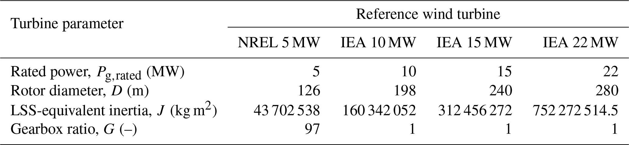
For convenience, empirical relations have been derived between the rotor diameters D, power ratings P_g,rated, and low-speed-shaft-equivalent inertias J of the turbines. By drawing such relations, it is possible to account for more turbine dimensions, power ratings, and inertias other than those of the reference turbines. To this end, the key properties of the reference wind turbines in Table 1 are used to obtain the following fitted functions:

$$\begin{array}{}\text{(1a)}& {\displaystyle }J\left(D\right)=\left(\mathrm{2.581}\cdot {\mathrm{10}}^{\mathrm{6}}\cdot {\mathrm{e}}^{\mathrm{0.02024}D}\right){\mathrm{kg}\mathrm{m}}^{\mathrm{2}},\text{(1b)}& {\displaystyle }{P}_{\mathrm{g},\mathrm{rated}}\left(D\right)=\left(\mathrm{1.491}\times {\mathrm{10}}^{\mathrm{6}}\times {\mathrm{e}}^{\mathrm{0.009613}D}\right)\mathrm{W},\text{(1c)}& {\displaystyle }\begin{array}{rl}J\left(P_{\mathrm{g},\mathrm{rated}}\right)& =\left(\mathrm{9.979}\times {\mathrm{10}}^{\mathrm{7}}{P}_{\mathrm{g},\mathrm{rated}}^{\mathrm{2}}+\mathrm{2.843}\right.\\ & \times {\mathrm{10}}^{\mathrm{8}}{P}_{\mathrm{g},\mathrm{rated}}\left.+\mathrm{2.424}\cdot {\mathrm{10}}^{\mathrm{8}}\right){\mathrm{kg}\mathrm{m}}^{\mathrm{2}}.\end{array}\end{array}$$

For the above fits, the coefficient of determination ℛ²>0.99 is ensured.

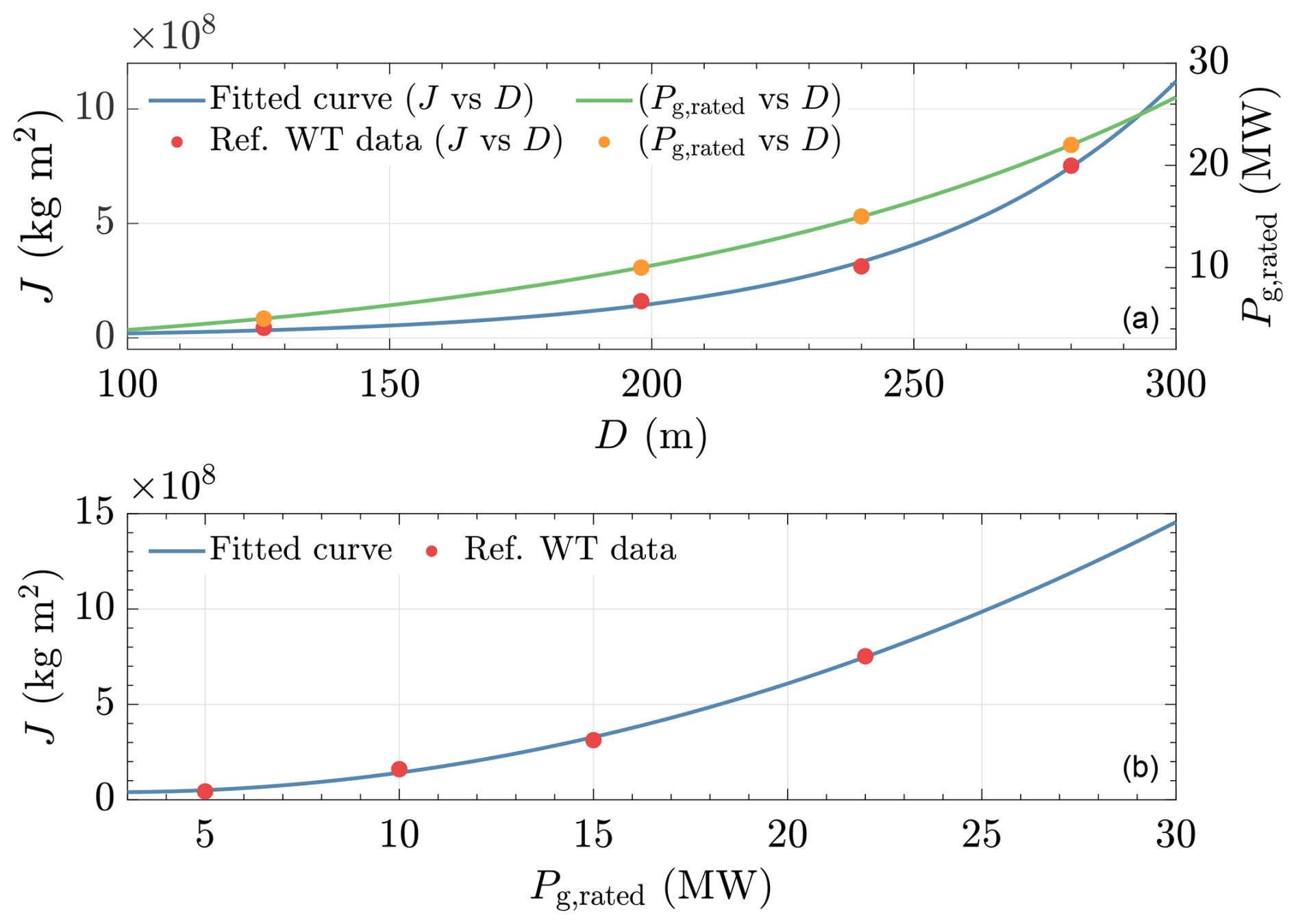
Figure 1 Curve-fitting results. Reference wind turbine data points are depicted by the dots, and the fitted curves are indicated by the lines. Panel (a) is the mapping from the rotor diameter to the inertia (left y axis) and rated generator power (right y axis). Panel (b) is the mapping from the rated generator power to the inertia.

2.3 Assumptions

• Assumption 1. The power coefficient represents the exact steady-state aerodynamic characteristics of the actual rotor.

• Assumption 2. In the low-fidelity simulations provided throughout this study, the power coefficient of all the considered reference wind turbines (see Table 1) is equal to that of the National Renewable Energy Laboratory (NREL) 5 MW reference wind turbine so as to enable a clear analysis and comparison of the results between the various considered turbines.

• Assumption 3. The drivetrain inertia value at the low-speed shaft side is assumed to be an a priori known parameter.

3 Closed-loop wind turbine model and rotor-effective wind speed estimation framework

Figure 2 presents the overall scheme considered in this work, in which the wind turbine is controlled by a partial-load controller along with a power balance wind speed estimator. The wind speed estimator, being the main focus of the analysis in this work, is connected in an open-loop system to the closed-loop system. The red block represents the wind turbine, the green block contains the controller, and the blue block is the power balance wind speed estimator considered in this study.

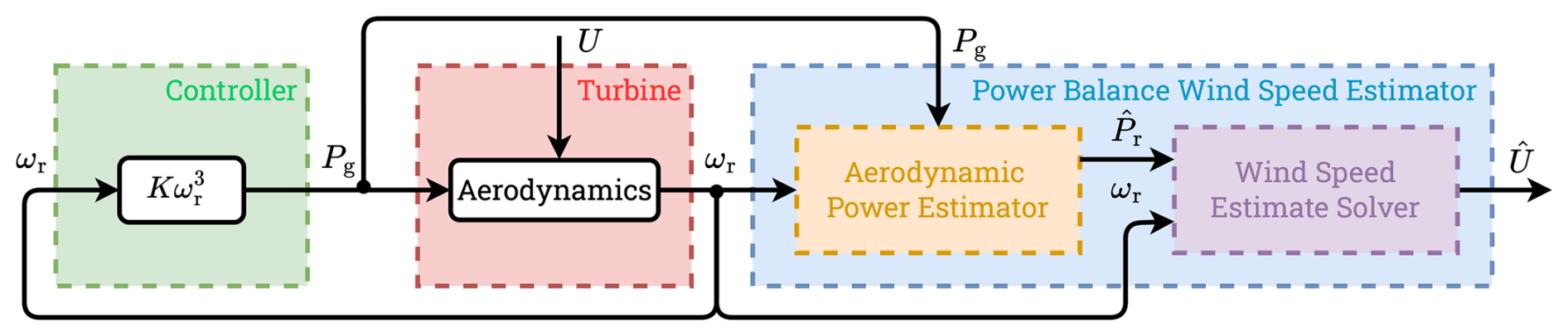
Figure 2 The general scheme of the power balance wind speed estimation considered in this study. The wind turbine (red block) is operated in a closed loop with a $K{\mathit{\omega }}_{\mathrm{r}}^{\mathrm{3}}$ controller (green block), whereas the power balance wind speed estimator (blue block) is in an open-loop configuration with the turbine. The power balance wind speed estimator is subdivided into the aerodynamic power estimator (yellow block) and wind speed estimate solver (purple block).

Section 3.1 and 3.2 provide the required theory used in this paper by outlining the first two subsystems, followed by defining the wind speed estimator. Then Sect. 3.3 addresses the decomposition of the estimator into several subcomponents, providing a framework for the remainder of the work presented in this paper.

3.1 Single-degree-of-freedom wind turbine model and optimal controller

In this work, single-degree-of-freedom power balance drivetrain dynamics are considered to be a simplified representation of a wind turbine as follows:

$$\begin{array}{}\text{(2)}& J{\mathit{\omega }}_{\mathrm{r}}\left(t\right){\dot{\mathit{\omega }}}_{\mathrm{r}}\left(t\right)=P_{\mathrm{r}}\left(t\right)-P_{\mathrm{g}}\left(t\right)/{\mathit{\eta }}_{\mathrm{g}},\end{array}$$

where J∈ℝ is the low-speed-shaft (LSS)-equivalent inertia, ω_r∈ℝ the rotor angular speed, and P_g∈ℝ the generated power with the corresponding generator efficiency factor ${\mathit{\eta }}_{\mathrm{g}}\in (\mathrm{0},\mathrm{1}]$. The aerodynamic power is given by the following nonlinear relation:

$$\begin{array}{}\text{(3)}& P_{\mathrm{r}}\left(t\right)={\displaystyle \frac{\mathrm{1}}{\mathrm{2}}}\mathit{\rho }{A}_{\mathrm{r}}{C}_{\mathrm{p}}\left(\mathit{\lambda }\right(t),\mathit{\beta }(t\left)\right)U(t{)}^{\mathrm{3}},\end{array}$$

in which ρ∈ℝ denotes the air density, A_r∈ℝ the rotor area, U∈ℝ the REWS (Soltani et al., 2013), and β∈ℝ the blade pitch angle. The power coefficient $C_{\mathrm{p}}:{\mathbb{R}}^{\mathrm{2}}\to \mathbb{R}$ is a nonlinear mapping from β and the non-dimensional tip-speed ratio (TSR), defined as

$$\begin{array}{}\text{(4)}& \mathit{\lambda }\left(t\right)={\displaystyle \frac{{\mathit{\omega }}_{\mathrm{r}}\left(t\right)R}{U\left(t\right)}},\end{array}$$

with R∈ℝ as the rotor radius.

• Remark 1. The power coefficient considered in this work does not take into account the aerodynamic effects due to structural deformations, e.g., those associated with bend–twist coupling of the blades. Had this been the case, changes in local blade sections' angle of attack are expected, and different combinations of ω_r and U, although they correspond to the same λ, might yield different power coefficients. This would render the $C_{\mathrm{p}}:{\mathbb{R}}^{\mathrm{2}}\to \mathbb{R}$ mapping between λ, β, and C_p inadequate such that $C_{\mathrm{p}}:{\mathbb{R}}^{\mathrm{3}}\to \mathbb{R}$ mapping is needed (i.e., $C_{\mathrm{p}}({\mathit{\omega }}_{\mathrm{r}},U,\mathit{\beta })$ instead of C_p(λ,β); see Lazzerini et al., 2024, and references therein). Nevertheless, without loss of generality, the mapping of the former is adopted for the sake of clarity of the analysis of this paper; thus, the C_p tables in this work are generated using a rigid-rotor assumption.

The drivetrain system outputs ω_r, which is then fed into the optimal torque controller (Bossanyi, 2000), often known as the “$K{\mathit{\omega }}_{\mathrm{r}}^{\mathrm{2}}$” controller. Although controllers performing better than $K{\mathit{\omega }}_{\mathrm{r}}^{\mathrm{2}}$, e.g., during transients, are available in the literature, partial-load controller design is not the main focus of this study. Hence, the $K{\mathit{\omega }}_{\mathrm{r}}^{\mathrm{2}}$ controller is deemed sufficient for the goal of this work. Having said that, this work is equally applicable to more advanced partial-load controllers available in the literature, such as tip-speed ratio tracking schemes, e.g., Brandetti et al. (2023) and Lazzerini et al. (2024). However, it should be noted that in the latter scheme, blade pitching is active in partial load. As the standard $K{\mathit{\omega }}_{\mathrm{r}}^{\mathrm{2}}$ scheme does not utilize blade pitch control, further study of the current estimation scheme under varying pitch angles is required and reserved for future work. Furthermore, constant pitch at a fine position of $\mathit{\beta }={\mathit{\beta }}^{\star }$ is used, and, for the sake of brevity, the notation $C_{\mathrm{p}}\left(\mathit{\lambda }\right):=C_{\mathrm{p}}(\mathit{\lambda },{\mathit{\beta }}^{\star })$ is used for the remainder of this paper. The $K{\mathit{\omega }}_{\mathrm{r}}^{\mathrm{2}}$ controller, in its generator-power equivalence, is expressed as

$$\begin{array}{}\text{(5)}& P_{\mathrm{g}}\left(t\right)={\mathit{\eta }}_{\mathrm{g}}K{\mathit{\omega }}_{\mathrm{r}}^{\mathrm{3}},\end{array}$$

where

$$K={\displaystyle \frac{\mathit{\pi }\mathit{\rho }{R}^{\mathrm{5}}{C}_{\mathrm{p}}^{\star }}{\mathrm{2}{{\mathit{\lambda }}^{\star }}^{\mathrm{3}}}}$$

is the optimal control gain. The notation λ^⋆ indicates the design TSR, corresponding to the optimal power coefficient, defined as $C_{\mathrm{p}}^{\star }:=C_{\mathrm{p}}\left({\mathit{\lambda }}^{\star }\right)$. Based on the expression in Eq. (5), in the remainder of this paper, as well as in Fig. 2, this optimal controller is referred to as “$K{\mathit{\omega }}_{\mathrm{r}}^{\mathrm{3}}$”.

3.2 Power balance wind speed estimation general concept

This section establishes the REWS estimation framework that forms the basis of the remainder of this paper. The rationale behind the power balance REWS estimator presented herein lies in the retrievability of wind speed information by asymptotic minimization of an error term between the aerodynamic power and its estimate, in which Assumption 1 holds, that is

$$\begin{array}{}\text{(6)}& U\left(t\right)=\underset{t\to \mathrm{\infty }}{lim}\underset{\widehat{U}\left(t\right)}{\arg \min }\left|e_{\mathrm{p}}\left(t\right)\right|,\end{array}$$

where $\widehat{U}\in \mathbb{R}$ denotes the REWS estimate. The notation e_p∈ℝ is the said estimation error, defined as

$$\begin{array}{}\text{(7)}& e_{\mathrm{p}}\left(t\right)=P_{\mathrm{r}}\left(t\right)-{\displaystyle \frac{\mathrm{1}}{\mathrm{2}}}\mathit{\rho }{A}_{\mathrm{r}}{C}_{\mathrm{p}}\left(\widehat{\mathit{\lambda }}\left(t\right)\right)\widehat{U}(t{)}^{\mathrm{3}},\end{array}$$

where the second term on the right-hand side of the equation is the aerodynamic power estimate based on Eq. (3), utilizing $\widehat{U}$ in place of U. The challenge of obtaining an estimate of P_r and solving the optimization problem of Eq. (6) is explained in further detail in the next section.

• Remark 2. Note that Eq. (6) will not be achieved in the presence of discrepancies between the utilized and actual C_p tables. Such disparities will lead to a biased wind speed estimate, as reported in Brandetti et al. (2022). Readers interested in the details of this ill-conditioning are therefore referred to that study.

3.3 Wind speed estimator subcomponent partitioning

Now that the closed-loop controlled wind turbine and wind speed estimation problem has been defined, the power balance REWS estimator explained in Sect. 3.2 can be partitioned into two subcomponents to allow for both rigorous analysis and effective estimation schemes: (i) aerodynamic power estimator and (ii) wind speed estimate solver. Figures 2 and 3 depict this partitioning, the latter of which details the possible techniques to realize these two subcomponents. Similar separation approaches have also been adopted in the literature, e.g., in Van Engelen and Van der Hooft (2003) and Østergaard et al. (2007). The current study provides a more in-depth analysis of the subcomponents.

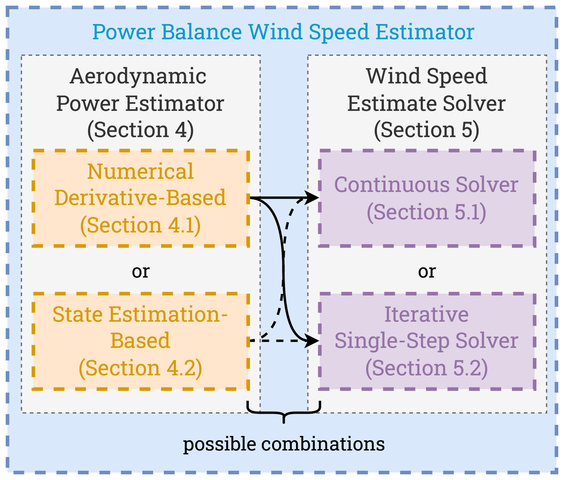
Figure 3 Power balance wind speed estimation partitioning. The left column contains the potential aerodynamic power estimators to be connected with the potential wind speed estimate solvers within the right column, thereby creating four possibilities for combining the two subcomponents.

The first block provides an estimate of the aerodynamic power, which – in contrast to the measured generator power – is more challenging to obtain, as is explained shortly. Fortunately, such information can still be obtained based on the available measurements and is the concern of the orange blocks in Figs. 2–3. By rearranging Eq. (2) and replacing specific variables with their estimated representations, one obtains

$$\begin{array}{}\text{(8)}& {\widehat{P}}_{\mathrm{r}}\left(t\right)=J{\mathit{\omega }}_{\mathrm{r}}\left(t\right){\widehat{\dot{\mathit{\omega }}}}_{\mathrm{r}}\left(t\right)+P_{\mathrm{g}}\left(t\right)/{\mathit{\eta }}_{\mathrm{g}}.\end{array}$$

Note that ${\widehat{P}}_{\mathrm{r}}$ and $P_{\mathrm{g}}/{\mathit{\eta }}_{\mathrm{g}}$ are equal to each other in steady state; however, due to the variable nature of the wind and rotor speed, omitting the rotor acceleration term entirely from this calculation means losing valuable dynamic information (Østergaard et al., 2007; Soltani et al., 2013). Therefore, taking into account the dynamics through the utilization of the rotor acceleration and the $J{\mathit{\omega }}_{\mathrm{r}}{\dot{\mathit{\omega }}}_{\mathrm{r}}$ terms enhances the accuracy of the REWS estimate during both steady-state and transient conditions.

In practice, however, rotor acceleration is not directly measurable, and it is challenging to obtain a good estimate of this quantity, ${\widehat{\dot{\mathit{\omega }}}}_{\mathrm{r}}$, due to the noisy nature of measured signals. To retrieve ${\widehat{\dot{\mathit{\omega }}}}_{\mathrm{r}}$, one may resort to numerical derivative methods of ω_r or state estimation methods, as depicted in Fig. 3. Subsequently, the aerodynamic power estimate ${\widehat{P}}_{\mathrm{r}}$ is obtained by solving Eq. (8).

• Remark 3. At this point, two aerodynamic power estimate terms have been introduced. One is ${\widehat{P}}_{\mathrm{r}}$, defined in Eq. (8), and the other is the second term on the right-hand side of Eq. (7). To prevent any confusion, the term “aerodynamic power estimate” is used to refer to the former, whereas the latter is from hereon referred to as the “$\widehat{U}$-dependent aerodynamic power estimate”.

Independent of how ${\widehat{P}}_{\mathrm{r}}$ is retrieved, such information, together with ω_r measurements, is then fed into the wind speed estimate solver subcomponent, indicated as the purple blocks in Fig. 3. Solving for the estimated wind speed is achieved in two ways in this work: the continuous (e.g., as used in Ortega et al., 2013, and Liu et al., 2022) and iterative single-step methods (e.g., through Newton–Raphson methods, as done in Van Engelen and Van der Hooft, 2003, and Boukhezzar and Siguerdidjane, 2011). A linear analysis of the continuous wind speed estimate solver in continuous time is provided, in which the stability properties of the linearized solver dynamics are derived. Furthermore, the effects of various discretization methods on the system, especially on the mentioned stability properties, are evaluated. The single-step approach solves the wind speed estimate in a similar way to the former method without the need for high solver gains, potentially causing stability issues when trying to obtain good estimation quality without phase lags. Its wind speed estimation quality is determined by the choice of error tolerance parameters and iteration budget.

The aforementioned options for each of the subcomponents, therefore, allow for several possible combinations in which the power balance wind speed estimator can be constructed, as illustrated in Fig. 3; however, the optimal combination has yet to be found. To this end, in Sects. 4 and 5, the derivations of the two aerodynamic power estimators and the wind speed estimate solvers are provided, respectively, where their performance is also evaluated.

4 Aerodynamic power estimator

As discussed previously, reconstructing aerodynamic power from available measurements is an essential step in obtaining an accurate REWS estimate in both steady-state and dynamic transient conditions. To this end, the most challenging part is obtaining an accurate estimate of the rotor acceleration ${\widehat{\dot{\mathit{\omega }}}}_{\mathrm{r}}$, which is the main concern of this section. Two approaches are considered herein. First, the numerical-derivative-based method is examined in Sect. 4.1. Later in Sect. 4.2, the state-estimation-based technique is discussed. In Sect. 4.3, the numerical comparisons for both methods are evaluated.

4.1 Numerical-derivative-based technique

To obtain an estimate of the rotor acceleration, a numerical derivative is applied to the measured ω_r. In the frequency domain, this is represented as follows:

$$\begin{array}{}\text{(9)}& {\widehat{\dot{\mathrm{\Omega }}}}_{\mathrm{r}}\left(s\right)=F_{\mathrm{nd},\mathrm{c}}(s,\mathit{\tau }){\mathrm{\Omega }}_{\mathrm{r}}\left(s\right),\end{array}$$

in which Ω_r and ${\widehat{\dot{\mathrm{\Omega }}}}_{\mathrm{r}}$, with slight abuse of notation for the latter, are the respective Laplace-transformed variables of ω_r and ${\widehat{\dot{\mathit{\omega }}}}_{\mathrm{r}}$. The transfer function

$$\begin{array}{}\text{(10)}& F_{\mathrm{nd},\mathrm{c}}(s,\mathit{\tau })={\displaystyle \frac{s}{\mathit{\tau }s+\mathrm{1}}}\end{array}$$

in Eq. (9) is the filtered derivative,² in accordance with the IEEE 421.5-2016 standard (IEEE, 2016), with a unity derivative gain. The parameter $\mathit{\tau }\in {\mathbb{R}}^{\ge \mathrm{0}}$ is the time constant of the numerical derivative.

In its implementation, the numerical derivative (Eq. 10) is discretized via the backward difference method. Thus, the discrete-time transfer function of the filter is

$$\begin{array}{}\text{(11)}& F_{\mathrm{nd},\mathrm{d}}(z,\mathit{\tau })=\left({\displaystyle \frac{\mathrm{1}}{\mathit{\tau }}}\right){\displaystyle \frac{\mathrm{1}-z^{-\mathrm{1}}}{\mathrm{1}+h/\mathit{\tau }-z^{-\mathrm{1}}}},\end{array}$$

where h denotes the sampling time.

As τ is the only tuning parameter for the filter (Eq. 11), it plays a crucial role. For instance, setting τ=0 casts F_nd,d into a pure differentiator. This enables infinite amplification at high frequencies (including noise), which is propagated to ${\widehat{\dot{\mathit{\omega }}}}_{\mathrm{r}}$, which is undesired. Having τ that is too large is also unwanted as ${\widehat{\dot{\mathit{\omega }}}}_{\mathrm{r}}$ and the subsequent ${\widehat{P}}_{\mathrm{r}}$ may become less accurate despite the better noise resilience. Calibration of τ is, therefore, a trade-off between having an accurate rotor acceleration estimate and good noise suppression. In the following section, a numerical demonstration of such a trade-off is performed and analyzed.

4.1.1 Time-constant selection: accuracy and noise propagation

As stated above, the choice of τ may be helpful in suppressing the effects of noisy measurements often encountered in real-world scenarios. To provide a clearer picture of this aspect, F_nd,d is applied to the discrete-time rendition of Eq. (9), resulting in the filtered and differentiated rotor speed

$$\begin{array}{}\text{(12)}& {\stackrel{\mathrm{̃}}{\widehat{\dot{\mathit{\omega }}}}}_{\mathrm{r}}\left(k\right)={\displaystyle \frac{{\stackrel{\mathrm{̃}}{\mathit{\omega }}}_{\mathrm{r}}\left(k\right)-{\stackrel{\mathrm{̃}}{\mathit{\omega }}}_{\mathrm{r}}(k-\mathrm{1})+\mathit{\tau }{\stackrel{\mathrm{̃}}{\widehat{\dot{\mathit{\omega }}}}}_{\mathrm{r}}(k-\mathrm{1})}{\mathit{\tau }+h}},\end{array}$$

with

$$\begin{array}{}\text{(13)}& {\stackrel{\mathrm{̃}}{\mathit{\omega }}}_{\mathrm{r}}\left(k\right)={\mathit{\omega }}_{\mathrm{r}}\left(k\right)+v_{{\mathit{\omega }}_{\mathrm{r}}}\left(k\right)\end{array}$$

as the noisy rotor speed signal, where $v_{{\mathit{\omega }}_{\mathrm{r}}}\sim (\mathrm{0},{\mathit{\sigma }}_{v_{{\mathit{\omega }}_{\mathrm{r}}}}^{\mathrm{2}})$ is an additive Gaussian white noise with a mean of zero and variance ${\mathit{\sigma }}_{v_{{\mathit{\omega }}_{\mathrm{r}}}}^{\mathrm{2}}$.

The impact of the noise propagated from ${\stackrel{\mathrm{̃}}{\mathit{\omega }}}_{\mathrm{r}}$ will affect the aerodynamic power estimate, as made evident in the following relation, obtained by substituting Eqs. (12)–(13) into Eq. (8):

$$\begin{array}{}\text{(14)}& {\widehat{P}}_{\mathrm{r}}\left(k\right)=J{\stackrel{\mathrm{̃}}{\mathit{\omega }}}_{\mathrm{r}}\left(k\right){\stackrel{\mathrm{̃}}{\widehat{\dot{\mathit{\omega }}}}}_{\mathrm{r}}\left(k\right)+P_{\mathrm{g}}\left(k\right)/{\mathit{\eta }}_{\mathrm{g}}.\end{array}$$

Note that the equation contains a multiplication between ${\stackrel{\mathrm{̃}}{\mathit{\omega }}}_{\mathrm{r}}$ and ${\stackrel{\mathrm{̃}}{\widehat{\dot{\mathit{\omega }}}}}_{\mathrm{r}}$. This implies that the noise the former contains is multiplied by the noise it propagated to the latter from the previous time step. This introduces a biased ${\widehat{P}}_{\mathrm{r}}$ that depends on the noise variance because the product of a noise sequence with itself, although it has a mean of zero, will give a nonzero mean.³ A chosen τ may lessen the effects of such noise propagation but may deteriorate ${\widehat{P}}_{\mathrm{r}}$ estimation performance and is a trade-off.

To numerically demonstrate the effect of noisy measurements on Eq. (14), 400 s simulations, sampled at h=0.02 s, were run for time constants and noise variances of $\mathit{\tau }\in [\mathrm{0},{\mathrm{10}}^{-\mathrm{1}}]$ s and ${\mathit{\sigma }}_{v_{{\mathit{\omega }}_{\mathrm{r}}}}^{\mathrm{2}}\in [{\mathrm{10}}^{-\mathrm{6}},{\mathrm{10}}^{-\mathrm{2}}]$ rad² s⁻², respectively. In addition, the inertia value of the NREL 5 MW is used (see Table 1) under steady-state operating conditions ${\stackrel{\mathrm{‾}}{\mathit{\omega }}}_{\mathrm{r}}=\mathrm{0.8}$ rad s⁻¹ and ${\stackrel{\mathrm{‾}}{P}}_{\mathrm{g}}=\mathrm{1.548}$ MW, the latter of which is computed using Eq. (5) with $C_{\mathrm{p}}^{\star }=\mathrm{0.469}$, ${\mathit{\lambda }}^{\star }=\mathrm{6.53}$, and η_g=0.94. Figure 4 summarizes the statistical results of these simulations, where ${\mathit{\mu }}_{{\widehat{P}}_{\mathrm{r}}}$ is the mean of the aerodynamic power estimate.

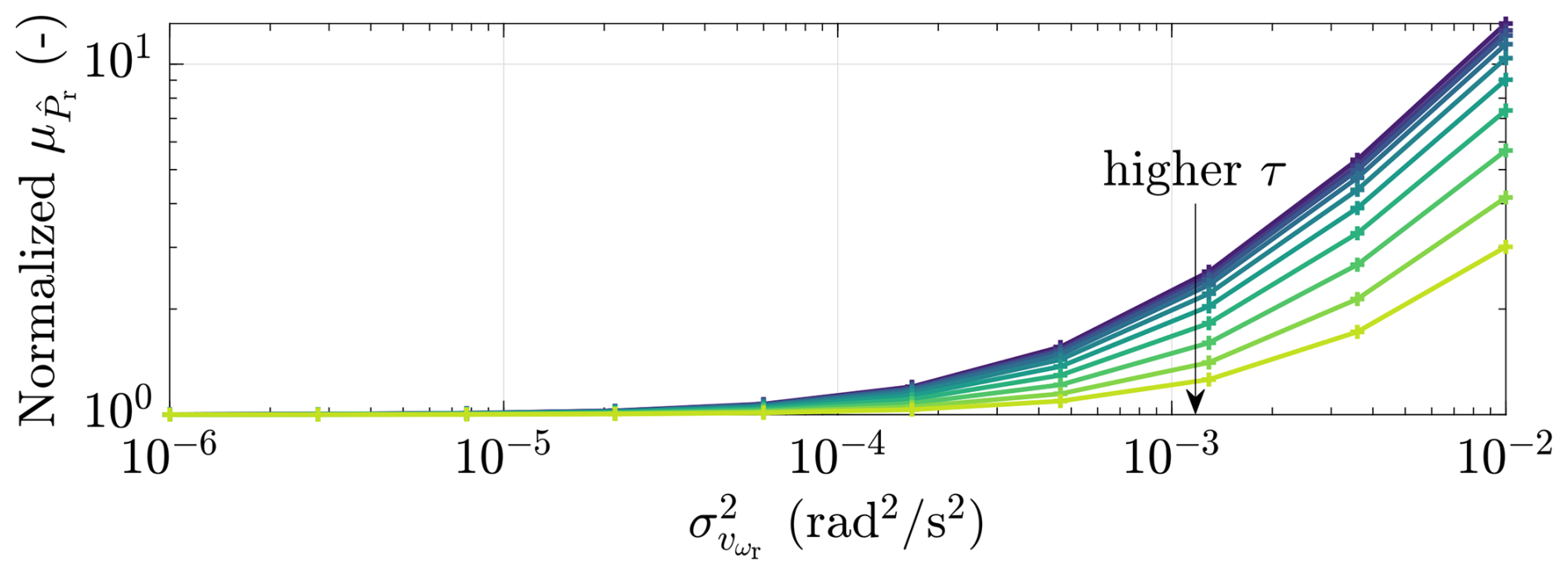
Figure 4 The mean of the aerodynamic power estimate ${\mathit{\mu }}_{{\widehat{P}}_{\mathrm{r}}}$, normalized with respect to that of a noiseless case. It is shown that with a high noise variance ${\mathit{\sigma }}_{v_{{\mathit{\omega }}_{\mathrm{r}}}}^{\mathrm{2}}$, the noise propagated by the numerical derivative from ω_r into ${\widehat{\dot{\mathit{\omega }}}}_{\mathrm{r}}$ results in a high bias in ${\widehat{P}}_{\mathrm{r}}$. Nonetheless, the application of τ lessened the severity of the increased aerodynamic power estimation bias, shown by lower ${\mathit{\mu }}_{{\widehat{P}}_{\mathrm{r}}}$ as τ becomes higher.

It is apparent in the figure that greater noise variance leads to higher ${\mathit{\mu }}_{{\widehat{P}}_{\mathrm{r}}}$, representing added bias in the aerodynamic power estimate; nevertheless, employing high τ values alleviates such deterioration to some extent. Also implied in this observation is that using τ=0 s (i.e., using a pure differentiator) is not desirable, especially in highly noisy environments, as this would lead to an infinite amplification of high-frequency components. In conclusion, attention needs to be paid to noisy ω_r conditions as the resulting biased ${\widehat{P}}_{\mathrm{r}}$ may undermine the REWS estimation in the end.

4.2 State-estimation-based technique

Besides the aforementioned numerical derivative technique used to obtain ${\widehat{\dot{\mathit{\omega }}}}_{\mathrm{r}}$ and thus ${\widehat{P}}_{\mathrm{r}}$, state-estimation-based methods can also be employed. Obtaining ${\widehat{P}}_{\mathrm{r}}$ via state estimation can be more beneficial compared to the numerical derivative technique in terms of having the freedom to trade-off sensitivity to noisy measurements with responsiveness through estimation gain tuning; however, it might be more challenging in its implementation and calibration.

Despite the adopted power balance wind speed estimation framework, the state estimator employed in this section utilizes an internal model based on the torque balance variant of Eq. (2). Retaining the power variables in Eq. (2) would lead to the internal estimator dynamics being nonlinear such that it becomes necessary to obtain the Jacobians of the system – adding complexities to the observer design. Therefore, to provide an aerodynamic power estimate, a reformulation is performed to obtain a torque-based estimator. To this end, the internal model is described as the following dynamics:

$$\begin{array}{}\text{(15)}& {\dot{\mathit{\omega }}}_{\mathrm{r}}\left(t\right)={\displaystyle \frac{T_{\mathrm{r}}\left(t\right)-G{T}_{\mathrm{g}}\left(t\right)}{J}},\end{array}$$

where $G\in {\mathbb{R}}^{+}$ is the gearbox ratio of the drivetrain, $T_{\mathrm{r}}=P_{\mathrm{r}}/{\mathit{\omega }}_{\mathrm{r}}$ is the aerodynamic torque, and $T_{\mathrm{g}}=P_{\mathrm{g}}/\left({\mathit{\eta }}_{\mathrm{g}}{\mathit{\omega }}_{\mathrm{r}}G\right)$ is the generator torque.

The dynamics (Eq. 15) are then recast into the following discrete state-space form by employing forward Euler discretization:

$$\begin{array}{}\text{(16)}& \begin{array}{rl}{x}_{\mathrm{s}}(k+\mathrm{1})& =A_{\mathrm{s}}{x}_{\mathrm{s}}\left(k\right)+B_{\mathrm{s},\mathrm{u}}{u}_{\mathrm{s}}\left(k\right)+B_{\mathrm{s},\mathrm{d}}{d}_{\mathrm{s}}\left(k\right)+w_{{\mathit{\omega }}_{\mathrm{r}}}\left(k\right),\\ & y_{\mathrm{s}}\left(k\right)=C_{\mathrm{s}}{x}_{\mathrm{s}}\left(k\right)+v_{{\mathit{\omega }}_{\mathrm{r}}}\left(k\right),\end{array}\end{array}$$

with

$$x_{\mathrm{s}}={\mathit{\omega }}_{\mathrm{r}},u_{\mathrm{s}}=T_{\mathrm{g}},d_{\mathrm{s}}=T_{\mathrm{r}},\text{and}{y}_{\mathrm{s}}={\mathit{\omega }}_{\mathrm{r}}$$

as the state, input, disturbance, and output, respectively, and the state-space matrices

$$A_{\mathrm{s}}=\mathrm{1},B_{\mathrm{s},\mathrm{u}}=-h{J}^{-\mathrm{1}}G,B_{\mathrm{s},\mathrm{d}}=h{J}^{-\mathrm{1}},\text{and}{C}_{\mathrm{s}}=\mathrm{1},$$

where $\mathit{\{}{x}_{\mathrm{s}},u_{\mathrm{s}},d_{\mathrm{s}},y_{\mathrm{s}}\mathit{\}}\in \mathbb{R}$ and $\mathit{\{}{A}_{\mathrm{s}},B_{\mathrm{s},\mathrm{u}},B_{\mathrm{s},\mathrm{d}},C_{\mathrm{s}}\mathit{\}}\in \mathbb{R}$. Also included in Eq. (16) are the process noise $w_{{\mathit{\omega }}_{\mathrm{r}}}\sim (\mathrm{0},{\mathit{\sigma }}_{w_{{\mathit{\omega }}_{\mathrm{r}}}}^{\mathrm{2}})$ with variance ${\mathit{\sigma }}_{w_{{\mathit{\omega }}_{\mathrm{r}}}}^{\mathrm{2}}$ and measurement noise $v_{{\mathit{\omega }}_{\mathrm{r}}}\sim (\mathrm{0},{\mathit{\sigma }}_{v_{{\mathit{\omega }}_{\mathrm{r}}}}^{\mathrm{2}})$ with variance ${\mathit{\sigma }}_{v_{{\mathit{\omega }}_{\mathrm{r}}}}^{\mathrm{2}}$, both assumed to be uncorrelated zero-mean Gaussian white noise. The aerodynamic torque is considered to be an unknown input and, therefore, a subject of the estimation. Thus, it is recast as a random-walk process (Verhaegen and Verdult, 2007) as follows:

$$\begin{array}{}\text{(17)}& T_{\mathrm{r}}(k+\mathrm{1})=T_{\mathrm{r}}\left(k\right)+w_{T_{\mathrm{r}}}\left(k\right),\end{array}$$

where $w_{T_{\mathrm{r}}}\sim (\mathrm{0},{\mathit{\sigma }}_{w_{T_{\mathrm{r}}}}^{\mathrm{2}})$ is a zero-mean Gaussian white noise sequence with variance ${\mathit{\sigma }}_{w_{T_{\mathrm{r}}}}^{\mathrm{2}}$, uncorrelated to $w_{{\mathit{\omega }}_{\mathrm{r}}}$ and $v_{{\mathit{\omega }}_{\mathrm{r}}}$. One advantage of treating T_r as a random-walk process is in the ease of design as no a priori information, such as aerodynamic torque coefficient, is needed. In particular, the Jacobian of this term is not necessary given that it is a nonlinear function of v and ω_r.

The general state-space expression for the state estimator – as depicted in Fig. 5, augmenting Eq. (17) to Eq. (16) and also including feedback from the measured system output y=ω_r – is written as follows:

$$\begin{array}{}\text{(18)}& \begin{array}{rl}\underset{{\widehat{\mathit{x}}}_{\mathrm{s},\mathrm{aug}}(k+\mathrm{1})}{\underbrace{\left[\begin{array}{c}{\widehat{x}}_{\mathrm{s}}(k+\mathrm{1})\\ {\widehat{T}}_{\mathrm{r}}(k+\mathrm{1})\end{array}\right]}}& =\underset{{\mathbf{A}}_{\mathrm{s},\mathrm{aug}}}{\underbrace{\left[\begin{array}{cc}{A}_{\mathrm{s}}& B_{\mathrm{s},\mathrm{d}}\\ \mathrm{0}& \mathrm{1}\end{array}\right]}}\underset{{\widehat{\mathit{x}}}_{\mathrm{s},\mathrm{aug}}\left(k\right)}{\underbrace{\left[\begin{array}{c}{\widehat{x}}_{\mathrm{s}}\left(k\right)\\ {\widehat{T}}_{\mathrm{r}}\left(k\right)\end{array}\right]}}+\underset{{\mathit{B}}_{\mathrm{s},\mathrm{aug}}}{\underbrace{\left[\begin{array}{c}{B}_{\mathrm{s},\mathrm{u}}\\ \mathrm{0}\end{array}\right]}}{T}_{\mathrm{g}}\left(k\right)\\ & +\underset{{\mathit{w}}_{\mathrm{s},\mathrm{aug}}\left(k\right)}{\underbrace{\left[\begin{array}{c}{w}_{{\mathit{\omega }}_{\mathrm{r}}}\left(k\right)\\ w_{T_{\mathrm{r}}}\left(k\right)\end{array}\right]}}+\mathit{L}\left(y\right(k)-{\widehat{y}}_{\mathrm{s}}(k\left)\right),\\ & {\widehat{y}}_{\mathrm{s}}\left(k\right)=\underset{{\mathit{C}}_{\mathrm{s},\mathrm{aug}}}{\underbrace{\left[\begin{array}{cc}{C}_{\mathrm{s}}& \mathrm{0}\end{array}\right]}}\underset{{\widehat{\mathit{x}}}_{\mathrm{s},\mathrm{aug}}\left(k\right)}{\underbrace{\left[\begin{array}{c}{\widehat{x}}_{\mathrm{s}}\left(k\right)\\ {\widehat{T}}_{\mathrm{r}}\left(k\right)\end{array}\right]}}+v_{{\mathit{\omega }}_{\mathrm{r}}}\left(k\right),\end{array}\end{array}$$

with $\mathit{L}=[L_{\mathrm{1}},L_{\mathrm{2}}{]}^{\top }$ as the observer gain vector. This gain can be determined by either a pole placement (Luenberger approach) or a Kalman design, the latter of which is able to provide minimum-variance unbiased state estimation by solving an algebraic Riccati equation involving the noise covariance matrices. However, because the former provides more freedom to define the pole locations of the state estimator according to one's own optimal performance criterion, in this study, L is determined by pole placement.

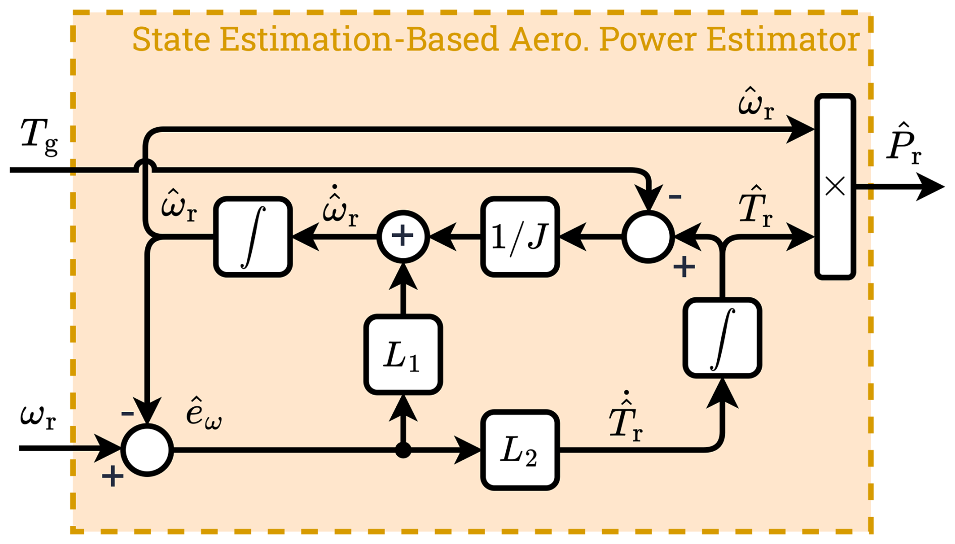
Figure 5 Internal structure of the state-estimation-based aerodynamic power estimator. Note that the aerodynamic power estimate ${\widehat{P}}_{\mathrm{r}}$ is the product of the rotor speed estimate ${\widehat{\mathit{\omega }}}_{\mathrm{r}}$ and aerodynamic torque estimate ${\widehat{T}}_{\mathrm{r}}$. See Remark 4 for more details.

• Remark 4. Similar to the numerical-derivative-based method, the state estimation scheme above can provide the aerodynamic power estimate by making use of the relation ${\widehat{P}}_{\mathrm{r}}=J{\widehat{\mathit{\omega }}}_{\mathrm{r}}{\widehat{\dot{\mathit{\omega }}}}_{\mathrm{r}}+P_{\mathrm{g}}/{\mathit{\eta }}_{\mathrm{g}}$. However, as in the state-estimation-based scheme considered in this section, the quantities ${\widehat{\mathit{\omega }}}_{\mathrm{r}}$ and ${\widehat{T}}_{\mathrm{r}}$ are accessible directly from the augmented state vector ${\widehat{\mathit{x}}}_{\mathrm{s},\mathrm{aug}}$ such that the aerodynamic power estimate can be computed straightforwardly via ${\widehat{P}}_{\mathrm{r}}={\widehat{\mathit{\omega }}}_{\mathrm{r}}{\widehat{T}}_{\mathrm{r}}$. Thus, this approach is considered for the remainder of this study.

In the aforementioned Luenberger approach, L needs to be designed such that ${\mathbf{A}}_{\mathrm{s},\mathrm{aug}}-\mathit{L}{\mathit{C}}_{\mathrm{s},\mathrm{aug}}$ has stable eigenvalues. Such a condition guarantees the convergence of $y-{\widehat{y}}_{\mathrm{s}}$ to zero given observable $({\mathbf{A}}_{\mathrm{s},\mathrm{aug}},{\mathit{C}}_{\mathrm{s},\mathrm{aug}})$. Evaluating this condition confirms that it is satisfied for $h{J}^{-\mathrm{1}}\ne \mathrm{0}$, which is always the case in practical scenarios.

With regard to the estimator's performance, having a closer look into the characteristic polynomial of ${\mathbf{A}}_{\mathrm{s},\mathrm{aug}}-\mathit{L}{\mathit{C}}_{\mathrm{s},\mathrm{aug}}$ may yield some new insights, e.g., how the design can be applied for different wind turbine power ratings. Furthermore, it is also somewhat known that the power rating of a wind turbine is associated with its dimension and, thus, inertial properties (Rodriguez et al., 2007), which, in this particular case, is the most influential as $h,G\ll J$. This indicates that a selected L suitable for a wind turbine might give a different performance when applied to another turbine with a different power rating. Therefore, it is crucial to find a gain-tailoring guideline so that identical state estimator performance among different power ratings or inertia values can be found.

The aforementioned considerations are addressed in the following sections: Sect. 4.2.1 provides the investigation into the characteristic polynomial of the estimator. A numerical demonstration is presented in Sect. 4.2.2 to compare the performance of the estimator with and without such a guideline.

4.2.1 State estimator characteristic polynomial

This section covers the analysis of the characteristic polynomial for the state-estimation-based aerodynamic power estimator laid out in the previous section. Investigation into such a characteristic polynomial informs one about how, for instance, the choice of estimator gain influences the natural frequency and damping of the estimator. The characteristic polynomial is derived as follows:

$$\begin{array}{}\text{(19)}& \text{det}(zI-{\mathbf{A}}_{\mathrm{s},\mathrm{aug}}+\mathit{L}{\mathit{C}}_{\mathrm{s},\mathrm{aug}})=z^{\mathrm{2}}+p_{\mathrm{1}}z+p_{\mathrm{2}}=\mathrm{0},\end{array}$$

in which the roots of the polynomial coefficients are parameterized as

$$\begin{array}{}\text{(20a)}& {\displaystyle }{p}_{\mathrm{1}}=\mathrm{2}(h{\mathit{\omega }}_{\mathrm{0}}{\mathit{\zeta }}_{\mathrm{0}}-\mathrm{1})=L_{\mathrm{1}}-\mathrm{2},\text{(20b)}& {\displaystyle }{p}_{\mathrm{2}}=\mathrm{1}-\mathrm{2}h{\mathit{\zeta }}_{\mathrm{0}}{\mathit{\omega }}_{\mathrm{0}}+h^{\mathrm{2}}{\mathit{\omega }}_{\mathrm{0}}^{\mathrm{2}}=\mathrm{1}-L_{\mathrm{1}}+{\displaystyle \frac{h}{J}}{L}_{\mathrm{2}},\end{array}$$

where ω₀ and ζ₀ are the respective natural frequency and damping ratio of the continuous-time characteristic equation⁴, which by further manipulation of Eq. (20) leads to

$$\begin{array}{}\text{(21a)}& {\displaystyle }{\mathit{\omega }}_{\mathrm{0}}=\sqrt{{\displaystyle \frac{L_{\mathrm{2}}}{hJ}}},\text{(21b)}& {\displaystyle }{\mathit{\zeta }}_{\mathrm{0}}={\displaystyle \frac{L_{\mathrm{1}}}{\mathrm{2}h{\mathit{\omega }}_{\mathrm{0}}}}.\end{array}$$

It is directly evident from the above equations that to maintain constant ω₀ and ζ₀ for a range of different turbines, the ratio $L_{\mathrm{2}}/J$ needs to be kept constant under the assumption that L₁ and h are equal for all turbines. Furthermore, it is more insightful to express L₁ and L₂ in terms of ω₀ and ζ₀ by rearranging Eq. (21) as follows:

$$\begin{array}{}\text{(22a)}& {\displaystyle }{L}_{\mathrm{1}}=\mathrm{2}h{\mathit{\zeta }}_{\mathrm{0}}{\mathit{\omega }}_{\mathrm{0}},\text{(22b)}& {\displaystyle }{L}_{\mathrm{2}}=hJ{\mathit{\omega }}_{\mathrm{0}}^{\mathrm{2}}.\end{array}$$

The relation above allows one to determine both gains based on specified ω₀ and ζ₀, but most importantly, it becomes clear that L₂ needs to be tailored based on the turbine inertia, especially if one wants to apply the estimator to different turbine sizes and power ratings, as discussed in the previous section. In the following section, how this gain is tailored to a range of wind turbine inertias is discussed, and a numerical demonstration is also provided.

4.2.2 Constant- and tailored-estimator-gain comparison

To numerically demonstrate the performance difference between constant and tailored L₂ over the considered range of turbines, 800 s simulations (sampled at h=0.02 s) are performed with a turbulent wind with a mean speed U_h=7.5 m s⁻¹ and an intensity I_T=4 %. The drivetrain dynamics (Eq. 2) in the closed-loop system with the controller (Eq. 5) are incorporated to represent the wind turbine. A total of 10 wind turbines within the $P_{\mathrm{g},\mathrm{rated}}\in [\mathrm{5},\mathrm{25}]$ MW range are considered, and the inverse of Eq. (1b) is used to obtain $R=D/\mathrm{2}$ from the specified P_g,rated, e.g., to compute TSR and the optimal mode gain K.

Their estimator gains are subsequently obtained using Eq. (22), in which ω₀=25 rad s⁻¹ and ζ₀=1 are chosen and, as shown later, result in satisfactory estimator performance. The J values derived from Eq. (1c) for the selected P_g,rated range are subsequently substituted to Eq. (22b) to adjust L₂ values⁵. For the constant-gain case, L₂ computed for $P_{\mathrm{g},\mathrm{rated}}=\mathrm{5}$ MW is considered for all turbines. No noise is assumed for ω_r measurements for the sake of simplicity in this demonstration; nevertheless, similar conclusions can be derived under noisy measurements.

Figure 6 summarizes the key statistical results of the simulations, being the absolute means ($\left|{\mathit{\mu }}_{(•)}\right|$) and standard deviations (σ_(•)) of the rotor speed, aerodynamic torque, and aerodynamic power estimation errors, ${\mathit{\omega }}_{\mathrm{r}}-{\widehat{\mathit{\omega }}}_{\mathrm{r}}$, $T_{\mathrm{r}}-{\widehat{T}}_{\mathrm{r}}$, and $P_{\mathrm{r}}-{\widehat{P}}_{\mathrm{r}}$, respectively. In general, it is observed from the figure that, compared with the tailored-gain case, the use of constant gain deteriorates the absolute means and standard deviations as the power rating increases. However, an exception applies for ${\mathit{\sigma }}_{T_{\mathrm{r}}-{\widehat{T}}_{\mathrm{r}}}$ and ${\mathit{\sigma }}_{P_{\mathrm{r}}-{\widehat{P}}_{\mathrm{r}}}$, where similar results are depicted for both cases.

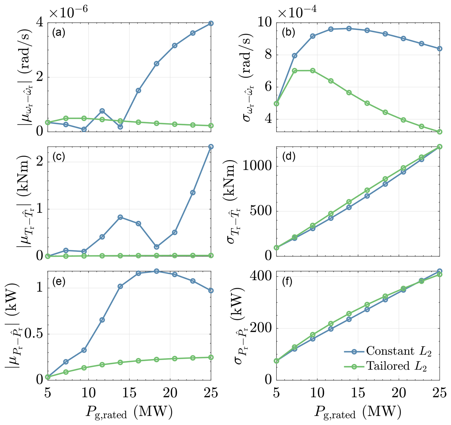
Figure 6 Statistical assessment results of the constant (blue) and tailored (green) Luenberger estimator's L₂ gain based on the power rating (and inertia) of the turbines. Absolute errors of the rotor speed, aerodynamic torque, and aerodynamic power estimates (a, c, e) of the constant-L₂ strategy tend to be much higher than those of the tailored gain. Significant difference in the standard deviations of these errors (b, d, f) is only shown for the rotor speed estimation, whereas those of the aerodynamic torque and power are comparable. These results imply that appropriate gain adjustment based on the power rating of the corresponding turbine is imperative.

The observation from the above demonstration motivates the need to set a new standard, i.e., by employing L₂ tailoring based on the power rating and consequent drivetrain inertia of the considered turbines, which provides a convenient means to calibrate state-estimation-based aerodynamic power estimation. As shown later, such a gain tailoring – and more importantly, the state-estimation-based aerodynamic power estimator – leads to faster (less phase lag) and more noise-resilient wind speed estimation.

4.3 Aerodynamic power estimation technique comparison

With the numerical derivative and state estimation approaches to estimating aerodynamic power presented in the previous sections, this section is now dedicated to comparing both methods. To this end, simulations with the same turbulent wind setting as in Sect. 4.2.2 are run, where a wind turbine of $P_{\mathrm{g},\mathrm{rated}}=\mathrm{15}$ MW, representing a “mid-sized” turbine in the considered turbine range, is utilized. In addition, noisy rotor speed measurements are assumed, with ${\mathit{\sigma }}_{v_{{\mathit{\omega }}_{\mathrm{r}}}}^{\mathrm{2}}={\mathrm{10}}^{-\mathrm{6}}$ rad² s⁻².

Two strategies for obtaining ${\widehat{P}}_{\mathrm{r}}$ are compared:

1. The first strategy is to use the filtered derivative F_nd,d introduced in Sect. 4.1 to obtain ${\widehat{\dot{\mathit{\omega }}}}_{\mathrm{r}}$, followed by its substitution to Eq. (8), including ω_r and P_g measurements with known J according to Assumption 3. A time constant of τ=0.5 s is selected as it is considered a good trade-off between noise correlation, quality of the derivative, and noise amplification limitation.

2. The second strategy is to directly retrieve ${\widehat{P}}_{\mathrm{r}}$ through the state estimation method explained in Sect. 4.2 by multiplying ${\widehat{\mathit{\omega }}}_{\mathrm{r}}$ and ${\widehat{T}}_{\mathrm{r}}$ (see Remark 4). The gain L is computed by setting ω₀=25 rad s⁻¹ and ζ₀=1, as used in the previous section.

Figure 7 depicts the time series results of the simulation, where, for clarity, the results are only chosen for the timestamp t=200–250 s. In the figure, the actual aerodynamic power as a ground truth is indicated by the gray line. It can be seen that the aerodynamic power estimation result for the state-estimation-based method outperforms that of the numerical derivative method in terms of less noise propagation and phase lag.

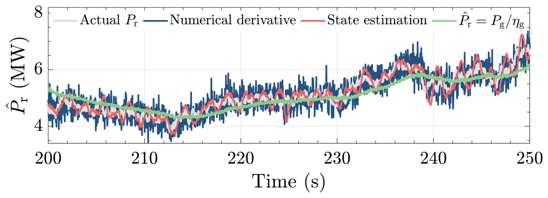
Figure 7 Comparison of aerodynamic power estimation methods. It is shown that the estimate obtained via the state-estimation-based technique (red line) has much less noise compared with that of the numerical derivative technique (blue line) while still maintaining high estimation accuracy. Also depicted is the aerodynamic power estimate determined using only the generated power (green line), which shows the worst-case phase lag with respect to the other methods, demonstrating the loss of information if rotor acceleration information is absent.

Note that, for the latter, increasing τ will result in less noise but increasing phase lag (Østergaard et al., 2007) as this will diminish and deteriorate the $J{\mathit{\omega }}_{\mathrm{r}}{\dot{\mathit{\omega }}}_{\mathrm{r}}$ estimate such that ${\widehat{P}}_{\mathrm{r}}\approx P_{\mathrm{g}}/{\mathit{\eta }}_{\mathrm{g}}$ (i.e., information will be lost). The case where $J{\mathit{\omega }}_{\mathrm{r}}{\dot{\mathit{\omega }}}_{\mathrm{r}}=\mathrm{0}$ such that ${\widehat{P}}_{\mathrm{r}}=P_{\mathrm{g}}/{\mathit{\eta }}_{\mathrm{g}}$ is demonstrated by the green line, which evidently shows a phase lag with respect to cases where the information of $J{\mathit{\omega }}_{\mathrm{r}}{\dot{\mathit{\omega }}}_{\mathrm{r}}$ is made available. It is concluded, therefore, that for the power balance REWS estimation scheme, the state-estimation-based aerodynamic power estimator is to be used for the remainder of this paper. Note that the performance of the state estimation method can be improved by further tuning ω₀ and ζ₀.

5 Wind speed estimate solver

Having a good estimate of the aerodynamic power is crucial for the second component of the overall power balance wind speed estimation scheme, which solves the effective wind speed estimate (see Fig. 2). Alluded to earlier in Sect. 3.3 and shown in Fig. 3, the two manners in which such a solver can be designed are detailed in the following sections. Section 5.1 discusses the continuous solver, where the linear state-space derivation of the solver is done, followed by frequency-domain analysis. Then, the stability of the solver in the discrete-time domain is discussed. Later, in Sect. 5.2, the iterative single-step algorithm is proposed as a promising alternative to the former.

5.1 Continuous solver

This section presents an analysis of the continuous manner of solving the wind speed estimate, given that the aerodynamic power estimate and rotor speed measurements are provided. Figure 8 depicts the internal structure of this continuous wind speed estimate solver, which is elaborated upon in the following.

Figure 8 Internal structure of the continuous wind speed estimate solver.

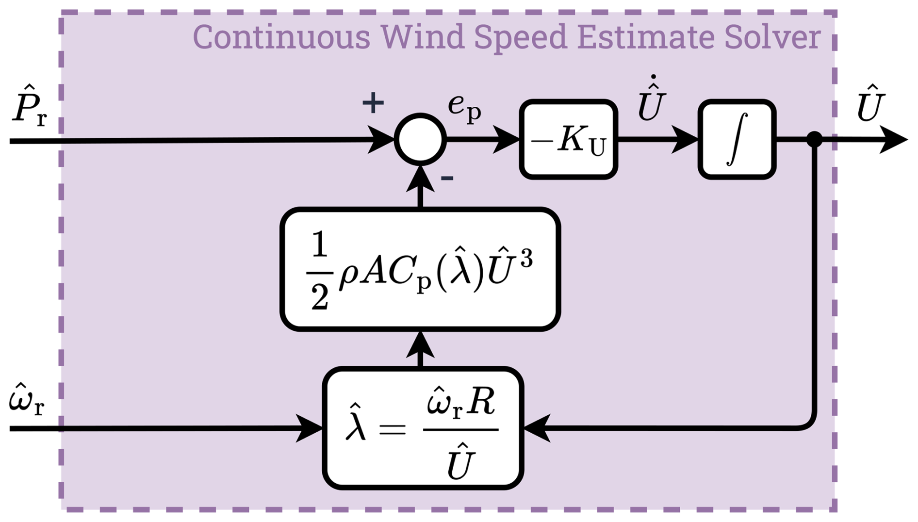
As laid out in Sect. 3.2, asymptotically minimizing the estimation error term e_p returns the wind speed estimate $\widehat{U}$, which converges to the actual wind speed over time as per the definition in Eq. (6). Such an integration operation enables the wind speed estimate solver to be written as the following state transition equation:

$$\begin{array}{}\text{(23)}& \dot{\widehat{U}}\left(t\right)=-K_{\mathrm{U}}{e}_{\mathrm{p}}\left(t\right),\end{array}$$

with the integrator gain

$$\begin{array}{}\text{(24)}& K_{\mathrm{U}}={\displaystyle \frac{\mathit{\kappa }}{P_{\mathrm{g},\mathrm{rated}}}}\end{array}$$

determining the convergence rate. The notation $\mathit{\kappa }\in {\mathbb{R}}^{+}$ is a constant, and the rated generator power $P_{\mathrm{g},\mathrm{rated}}\in {\mathbb{R}}^{+}$ is used to convert e_p from wattage into the per-unit (p.u.) system.

As e_p has a nonlinear analytic definition (Eq. 7), the wind speed estimate solver in the continuous time is represented by the following nonlinear dynamics:

$$\mathcal{S}:\left\{\begin{array}{l}\dot{x}\left(t\right)=f\left(x\right(t),\mathit{u}(t\left)\right),\\ y\left(t\right)=g\left(x\right(t\left)\right),\end{array}\right.$$

with

$$x=\widehat{U},\mathit{u}={\left[{\widehat{P}}_{\mathrm{r}},{\widehat{\mathit{\omega }}}_{\mathrm{r}}\right]}^{\top },\text{and}y=\widehat{U}$$

as its state, input, and output vectors, respectively.

To proceed with the linear analysis, the first-order Taylor expansion of 𝒮 is derived, resulting in the following linear state-space system:

$$\begin{array}{}\text{(25)}& \begin{array}{rl}& \dot{x}\left(t\right)=Ax\left(t\right)+\mathit{B}\mathit{u}\left(t\right),\\ & y\left(t\right)=Cx\left(t\right),\end{array}\end{array}$$

with the state, input, and output matrices defined respectively by the following Jacobians:

$$\begin{array}{}\text{(26)}& \begin{array}{rl}& A={\left.{\displaystyle \frac{\partial f}{\partial x}}\right|}_{(\stackrel{\mathrm{‾}}{x},\stackrel{\mathrm{‾}}{\mathit{u}},\stackrel{\mathrm{‾}}{y})}=-{\displaystyle \frac{K_{\mathrm{U}}}{\mathrm{2}}}\mathit{\rho }{A}_{\mathrm{r}}{\stackrel{\mathrm{‾}}{\widehat{U}}}^{\mathrm{2}}\left(\mathrm{3}{C}_{\mathrm{p}}\left(\stackrel{\mathrm{‾}}{\widehat{\mathit{\lambda }}}\right)-\stackrel{\mathrm{‾}}{\widehat{\mathit{\lambda }}}{\displaystyle \frac{\partial C_{\mathrm{p}}}{\partial \widehat{\mathit{\lambda }}}}\right),\\ & \mathit{B}={\left.{\displaystyle \frac{\partial f}{\partial \mathit{u}}}\right|}_{(\stackrel{\mathrm{‾}}{x},\stackrel{\mathrm{‾}}{\mathit{u}},\stackrel{\mathrm{‾}}{y})}=-K_{\mathrm{U}}\left[\mathrm{1}-{\displaystyle \frac{\mathrm{1}}{\mathrm{2}}}\mathit{\rho }{A}_{\mathrm{r}}R{\stackrel{\mathrm{‾}}{\widehat{U}}}^{\mathrm{2}}{\displaystyle \frac{\partial C_{\mathrm{p}}}{\partial \widehat{\mathit{\lambda }}}}\right],\\ & C={\left.{\displaystyle \frac{\partial g}{\partial x}}\right|}_{(\stackrel{\mathrm{‾}}{x},\stackrel{\mathrm{‾}}{\mathit{u}},\stackrel{\mathrm{‾}}{y})}=\mathrm{1}.\end{array}\end{array}$$

Given the linearized dynamics above, it becomes compelling to examine the stability properties of the linear system. To this end, the next subsections provide frequency-domain stability and discretization-method analysis utilizing the above-derived linear system.

5.1.1 Frequency-domain stability analysis

In the previous section, the nonlinear dynamics of the continuous solver have been described, followed by their linear state-space rendition. Here, the stability of the solver is assessed via pole location investigation. Solving for $\mathit{G}\left(s\right)=Y\left(s\right)/\mathit{U}\left(s\right)=C(s-A{)}^{-\mathrm{1}}\mathit{B}$, one obtains the multiple-input single-output transfer matrix formulation of the state-space (Eq. 25) as follows:

$$\begin{array}{}\text{(27)}& \mathit{G}\left(s\right)={\displaystyle \frac{\mathit{N}}{D\left(s\right)}}.\end{array}$$

The notations N=B and D(s) are the respective numerators and denominator of the transfer functions above, with the former being a constant-gain vector, hence the independence from s. The latter is of interest, especially with regard to stability analysis.

The denominator of the transfer functions is

$$\begin{array}{}\text{(28)}& D\left(s\right)=s+\underset{p}{\underbrace{{\displaystyle \frac{K_{\mathrm{U}}}{\mathrm{2}}}\mathit{\rho }{A}_{\mathrm{r}}{\stackrel{\mathrm{‾}}{\widehat{U}}}^{\mathrm{2}}\left(\mathrm{3}{C}_{\mathrm{p}}\left(\stackrel{\mathrm{‾}}{\widehat{\mathit{\lambda }}}\right)-\stackrel{\mathrm{‾}}{\widehat{\mathit{\lambda }}}{\displaystyle \frac{\partial C_{\mathrm{p}}}{\partial \widehat{\mathit{\lambda }}}}\right)}},\end{array}$$

which, in order to guarantee stability, the left-half plane pole location p<0 must be satisfied such that

$$\begin{array}{}\text{(29)}& p=-\underset{p_c}{\underbrace{{\displaystyle \frac{K_{\mathrm{U}}}{\mathrm{2}}}\mathit{\rho }{A}_{\mathrm{r}}{\stackrel{\mathrm{‾}}{\widehat{U}}}^{\mathrm{2}}}}\left(\underset{p_a}{\underbrace{\mathrm{3}{C}_{\mathrm{p}}\left(\stackrel{\mathrm{‾}}{\widehat{\mathit{\lambda }}}\right)}}-\underset{p_b}{\underbrace{\stackrel{\mathrm{‾}}{\widehat{\mathit{\lambda }}}{\displaystyle \frac{\partial C_{\mathrm{p}}}{\partial \widehat{\mathit{\lambda }}}}}}\right)<\mathrm{0},\end{array}$$

with p_c>0. The inequality (Eq. 29) requires $p_a-p_b>\mathrm{0}$ to hold to ensure the pole stays within the left-half plane. This condition, which can be rewritten as

$$\begin{array}{}\text{(30)}& p_a>p_b\iff {\displaystyle \frac{\mathrm{3}}{\stackrel{\mathrm{‾}}{\widehat{\mathit{\lambda }}}}}{C}_{\mathrm{p}}\left(\stackrel{\mathrm{‾}}{\widehat{\mathit{\lambda }}}\right)>{\displaystyle \frac{\partial C_{\mathrm{p}}}{\partial \widehat{\mathit{\lambda }}}},\end{array}$$

is a well-known condition for global asymptotic stability in (improved) immersion and invariance wind speed estimator studies, e.g., Ortega et al. (2013) and Liu et al. (2022).

With the stability expression of Eq. (29) (or Eq. 30) at hand, a stability map under different operating conditions is made. For this purpose, the C_p table of the NREL 5 MW is taken. Figure 9 depicts the resulting stability region of the continuous wind speed estimate solver. The stable region is shown in green, whereas the unstable region is in blue. The left subfigure illustrates how the C_p contour is divided based on whether Eq. (29) (or Eq. 30) is satisfied. The blue dot shows the location of $C_{\mathrm{p}}^{\star }$, corresponding to the fine pitch β^⋆ (horizontal dashed line) and design TSR λ^⋆ (vertical dashed line). The operating conditions at the β^⋆ line are mapped on the right subfigure, resulting in a stability region representation in terms of U and ω_r. The solid blue line represents the λ^⋆ or $K{\mathit{\omega }}_{\mathrm{r}}^{\mathrm{3}}$ line, where maximum power extraction occurs. As can be seen, the continuous wind speed estimate solver is stable for a large part of the turbine operational domain and, more importantly, along the optimal $K{\mathit{\omega }}_{\mathrm{r}}^{\mathrm{3}}$ line where the turbine operates in partial load in steady state.

However, as far as practicality is concerned, the effects of discrete-time implementations should extend the above continuous-time analysis. A discretization method, for instance, might not preserve the stability properties obtained in the continuous-time domain (Åström and Wittenmark, 2011). Moreover, different estimator gain κ values influence the stability region. These aspects are the main concerns in the next section.

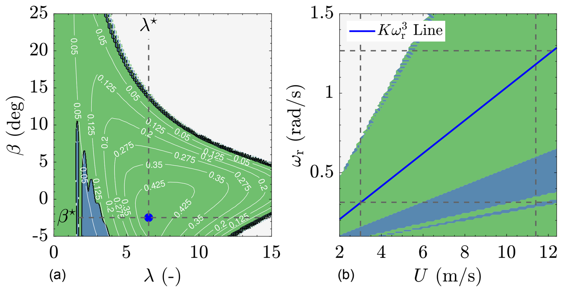
Figure 9 Stability region of the continuous wind speed estimate solver in the continuous time G(s), where the condition p<0 in Eq. (29) is satisfied (indicated in green, otherwise in blue). The left subfigure shows the different C_p levels for the NREL 5 MW turbine (solid white lines), with $C_{\mathrm{p}}^{\star }$ indicated by the blue dot. The right subfigure shows the mapping of the stability region in terms of wind speed U and rotor speed ω_r for the fine pitch angle β^⋆. The solid blue line is the partial-load regime, where the $K{\mathit{\omega }}_{\mathrm{r}}^{\mathrm{3}}$ controller is active. Also shown for completeness are the dashed black lines, indicating the lower and upper bounds for the rotor speed, as well as cut-in and rated wind speeds.

5.1.2 Solver discretization and instability

In this section, the stability of the continuous wind speed estimate solver (Eq. 27) in the discrete time is discussed. The three most common discretization methods are considered to be the following (Åström and Wittenmark, 2011):

1. the forward Euler (FE) method, with the following s- to z-domain transformation,

   $$\begin{array}{}\text{(31)}& s_{\mathrm{FE}}^{\prime }={\displaystyle \frac{z-\mathrm{1}}{h}};\end{array}$$

2. the backward difference (BD) method, with the following transformation,

   $$\begin{array}{}\text{(32)}& s_{\mathrm{BD}}^{\prime }={\displaystyle \frac{z-\mathrm{1}}{zh}};\end{array}$$

3. the Tustin (TU) method, with

   $$\begin{array}{}\text{(33)}& s_{\mathrm{TU}}^{\prime }={\displaystyle \frac{\mathrm{2}}{h}}{\displaystyle \frac{z-\mathrm{1}}{z+\mathrm{1}}}\end{array}$$

   as the corresponding s- to z-domain transformation.

Substituting any of the above discretization methods into G(s) results in the following general discrete-time approximation representation:

$$\begin{array}{}\text{(34)}& \mathit{G}(s=s^{\prime })=\mathit{H}\left(z\right)={\displaystyle \frac{\mathit{P}\left(z\right)}{Q\left(z\right)}},\end{array}$$

with P(z) denoting the numerators and Q(z) the denominator of the discrete-time transfer function H(z).

Similar to its continuous-time counterpart, discrete-time stability analysis only focuses on the poles of the system, i.e., whether they are within the unit disk, such that in the following study, only Q(z) is of interest (Åström and Wittenmark, 2011). Explicit representations of H(z), obtained by the discretization methods in Eqs. (31)–(33), are, therefore, provided below, and their corresponding stability condition derivation follows:

1. Using $s=s_{\mathrm{FE}}^{\prime }$ for the FE method, G(s) becomes

   $$\begin{array}{}\text{(35)}& {\mathit{H}}_{\mathrm{FE}}\left(z\right)={\displaystyle \frac{\mathit{N}h}{z+K_{\mathrm{U},\mathrm{h}}\frac{\mathrm{1}}{\mathrm{2}}\mathit{\rho }{A}_{\mathrm{r}}{\stackrel{\mathrm{‾}}{\widehat{U}}}^{\mathrm{2}}(p_a-p_b)-\mathrm{1}}},\end{array}$$

   with $K_{\mathrm{U},\mathrm{h}}=h{K}_{\mathrm{U}}$ (or, similarly, $K_{\mathrm{U},\mathrm{h}}=h\mathit{\kappa }/P_{\mathrm{g},\mathrm{rated}}$). From Eq. (35), the following inequality must hold for stability to hold:

   $$\begin{array}{}\text{(36)}& \left|\mathrm{1}-K_{\mathrm{U},\mathrm{h}}{\displaystyle \frac{\mathrm{1}}{\mathrm{2}}}\mathit{\rho }{A}_{\mathrm{r}}{\stackrel{\mathrm{‾}}{\widehat{U}}}^{\mathrm{2}}(p_a-p_b)\right|<\mathrm{1}.\end{array}$$

2. For the BD method, $s=s_{\mathrm{BD}}^{\prime }$ is used, and the following discrete transfer function is obtained:

   $$\begin{array}{}\text{(37)}& {\mathit{H}}_{\mathrm{BD}}\left(z\right)={\displaystyle \frac{\left(\mathit{N}h\right)z}{\left(\mathrm{1}+K_{\mathrm{U},\mathrm{h}}\frac{\mathrm{1}}{\mathrm{2}}\mathit{\rho }{A}_{\mathrm{r}}{\stackrel{\mathrm{‾}}{\widehat{U}}}^{\mathrm{2}}(p_a-p_b)\right)z-\mathrm{1}}},\end{array}$$

   with the following condition for stability:

   $$\begin{array}{}\text{(38)}& \left|{\displaystyle \frac{\mathrm{1}}{\mathrm{1}+K_{\mathrm{U},\mathrm{h}}\frac{\mathrm{1}}{\mathrm{2}}\mathit{\rho }{A}_{\mathrm{r}}{\stackrel{\mathrm{‾}}{\widehat{U}}}^{\mathrm{2}}(p_a-p_b)}}\right|<\mathrm{1}.\end{array}$$

3. Under the TU discretization, $s=s_{\mathrm{TU}}^{\prime }$ casts G(s) into

   $$\begin{array}{}\text{(39)}& {\mathit{H}}_{\mathrm{TU}}\left(z\right)={\displaystyle \frac{\frac{\mathit{N}h}{\mathrm{2}}(z+\mathrm{1})}{z+K_{\mathrm{U},\mathrm{h}}\frac{\mathrm{1}}{\mathrm{4}}\mathit{\rho }{A}_{\mathrm{r}}{\stackrel{\mathrm{‾}}{\widehat{U}}}^{\mathrm{2}}(p_a-p_b)(z+\mathrm{1})-\mathrm{1}}},\end{array}$$

   the stability of which is determined by the following inequality:

   $$\begin{array}{}\text{(40)}& \left|{\displaystyle \frac{\mathrm{1}-K_{\mathrm{U},\mathrm{h}}\frac{\mathrm{1}}{\mathrm{4}}\mathit{\rho }{A}_{\mathrm{r}}{\stackrel{\mathrm{‾}}{\widehat{U}}}^{\mathrm{2}}(p_a-p_b)}{\mathrm{1}+K_{\mathrm{U},\mathrm{h}}\frac{\mathrm{1}}{\mathrm{4}}\mathit{\rho }{A}_{\mathrm{r}}{\stackrel{\mathrm{‾}}{\widehat{U}}}^{\mathrm{2}}(p_a-p_b)}}\right|<\mathrm{1}.\end{array}$$

Note that the stability properties may now be influenced by the choice of sampling time h and gain κ (as P_g,rated is constant). Nevertheless, to better illustrate whether alterations in the stability region occur after discretization takes place, the stability conditions in Eqs. (36), (38), and (40) are plotted in a similar manner to Fig. 9, as explained in the following. Also considered are the following two arbitrary operating points (OPs) along the $K{\mathit{\omega }}_{\mathrm{r}}^{\mathrm{3}}$ line for a low and high partial-load wind speed:

$$\text{OP 1:}\left\{\begin{array}{l}\stackrel{\mathrm{‾}}{x}=\stackrel{\mathrm{‾}}{y}=\stackrel{\mathrm{‾}}{\widehat{U}}=\mathrm{4.5}\mathrm{m}/\mathrm{s},\\ \stackrel{\mathrm{‾}}{\mathit{u}}={\left[{\stackrel{\mathrm{‾}}{\widehat{P}}}_{\mathrm{r}},{\stackrel{\mathrm{‾}}{\mathit{\omega }}}_{\mathrm{r}}\right]}^{\top }=[\mathrm{3.263}\times {\mathrm{10}}^{\mathrm{5}}\mathrm{W},\mathrm{0.469}\mathrm{rad}{\mathrm{s}}^{-\mathrm{1}}{]}^{\top }\end{array}\right.$$

and

$$\text{OP 2:}\left\{\begin{array}{l}\stackrel{\mathrm{‾}}{x}=\stackrel{\mathrm{‾}}{y}=\stackrel{\mathrm{‾}}{\widehat{U}}=\mathrm{10.5}\mathrm{m}{\mathrm{s}}^{-\mathrm{1}},\\ \stackrel{\mathrm{‾}}{\mathit{u}}={\left[{\stackrel{\mathrm{‾}}{\widehat{P}}}_{\mathrm{r}},{\stackrel{\mathrm{‾}}{\mathit{\omega }}}_{\mathrm{r}}\right]}^{\top }=[\mathrm{4.145}\times {\mathrm{10}}^{\mathrm{6}}\mathrm{W},\mathrm{1.094}\mathrm{rad}{\mathrm{s}}^{-\mathrm{1}}{]}^{\top },\end{array}\right.$$

respectively, computed using the NREL 5 MW properties.

First, the stability region for the FE method, with $h=\mathrm{1}/\mathrm{50}$ s constant for all evaluations, is examined. Figure 10 depicts the resulting stability assessment, which illustrates the deterioration of the stability region of the FE method as κ increases, affecting the partial-load operations (solid blue line), e.g., OP 2 (red dot). Although not shown in the figure, even higher κ may affect low-wind-speed operations. This observation, therefore, concludes that one's choice of discretization method results in a performance limitation of the wind speed estimate solver in terms of an existing “upper bound” for the magnitude of κ. Nevertheless, a compromise can be made to improve the stability of the FE method by increasing sampling frequency (i.e., lowering h) proportional to the increase in κ to maintain constant K_U,h. However, increasing the sampling frequency does not eliminate the presence of a κ “upper bound”; moreover, the extent to which such a frequency can be increased is practically limited as a result, e.g., hardware capabilities. Therefore, a more feasible solution is to adopt different discretization methods while leaving the sampling frequency unchanged.

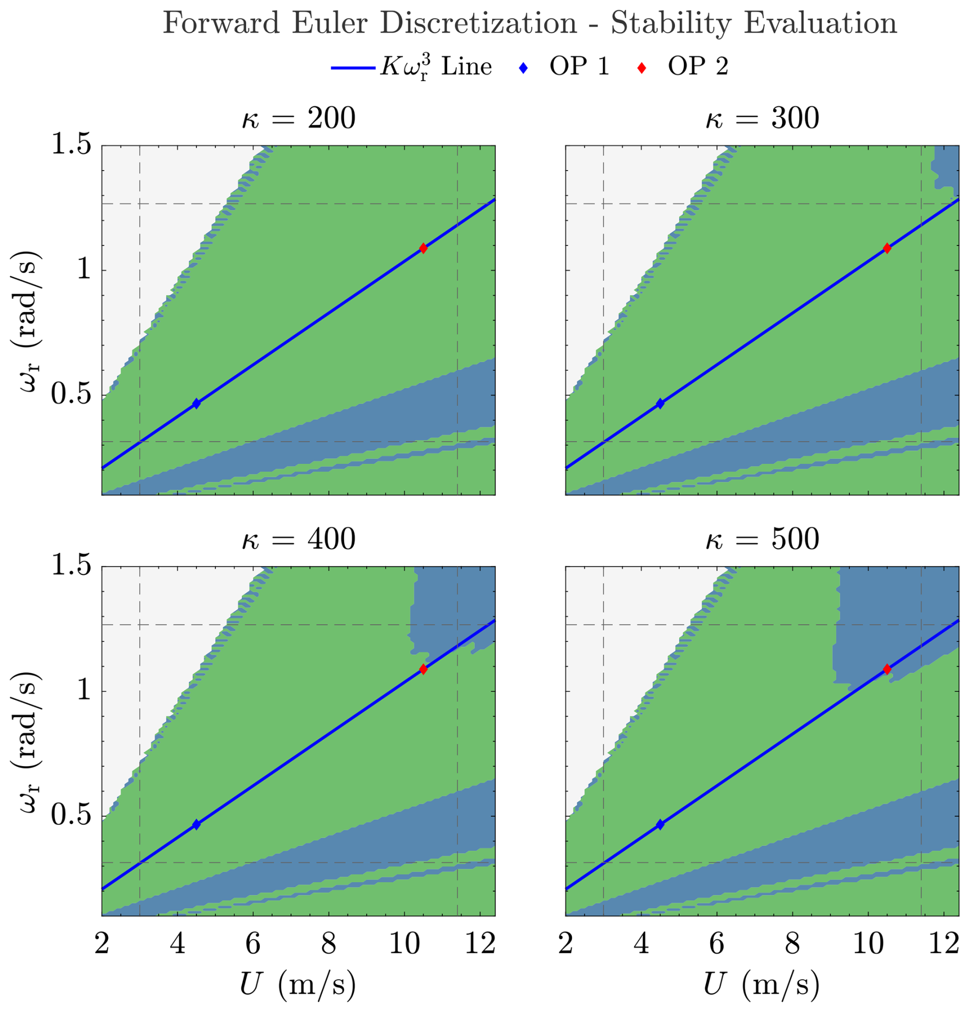
Figure 10 Unstable region's (blue area) growth in H_FE(z) with increasing $\mathit{\kappa }=\mathit{\{}\mathrm{200},\mathrm{300},\mathrm{400},\mathrm{500}\mathit{\}}$ using $h=\mathrm{1}/\mathrm{50}$ s of sampling time and the forward Euler discretization method.

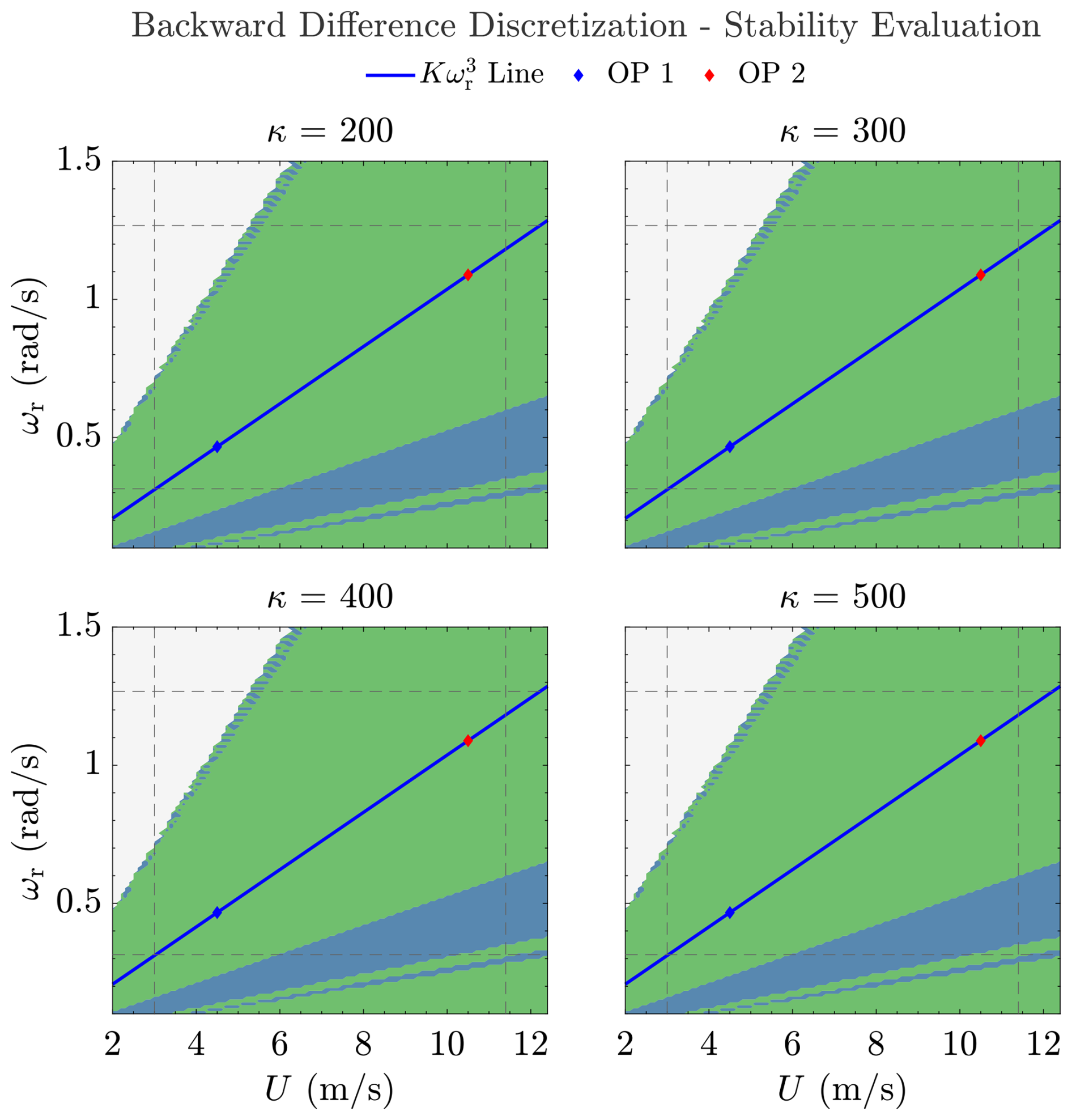
Figure 11 Stability region of H_BD(z) with increasing $\mathit{\kappa }=\mathit{\{}\mathrm{200},\mathrm{300},\mathrm{400},\mathrm{500}\mathit{\}}$ using $h=\mathrm{1}/\mathrm{50}$ s of sampling time and the backward difference (BD) discretization method. An identical graphical evaluation is obtained for the Tustin-discretized system H_TU(z) for the selected gains.

Figure 11 makes it clear that the BD method, in contrast to the FE method, does not result in the change of the stability characteristics of the continuous system when converted into the discrete system for the considered κ values. Remarkably, if κ is further increased, the pole of the discrete-time system H_BD(z) moves even farther away from the edge of the unit circle (as implied in Eq. 38, theoretically leading to increased stability for increasing gains).

Similar to the BD method, the TU method gain increase will lead to the discrete-time pole moving closer to the origin, but under the same gain, the pole in the TU method will be closer to the origin than in the BD method. This is because with the TU method, higher gains simultaneously lower the numerator and increase the denominator of the discrete pole, as can be implied from Eq. (40). Regardless, for the considered κ, the stability region of the TU-discretized system H_TU(z) is identical to that of G(s). It is therefore worth noting that although Fig. 11 shows the stability characteristics of H_BD(z) for the given gains, those of H_TU(z) would give identical representations; therefore, no dedicated figure is provided for the latter for brevity.

To summarize, the BD and TU methods are the preferred discretization techniques for discrete-time implementations of the continuous wind speed estimate solver in that the stability condition from the continuous-time system is preserved. Given present-day computational resources and readily available discretization methods in popular software packages, the selection for each of the methods is inconsequential from an implementation perspective. Therefore, later in Sect. 5.3, a time series numerical comparison is performed to determine the most suitable approach, also including the iterative single-step solver explained in the next section.

5.2 Iterative single-step solver

Besides the continuous wind speed estimate solver in the previous section, iterative numerical methods can also be employed to solve for the wind speed estimate. A well-known iterative method for this purpose is the Newton–Raphson method, as used in the work of Van Engelen and Van der Hooft (2003) and Boukhezzar and Siguerdidjane (2011). This iterative algorithm finds the roots of a function given an initial guess and makes use of the gradient of the function. The reliance on such a gradient, however, adds an additional layer of complexity in this case in that an extra look-up table other than that for the C_p table is needed. Moreover, the use of this extra look-up table would increase the computational burden per iteration within the algorithm. Fortunately, the definition of wind speed estimate, being an integration of the estimation error e_p over time multiplied by a gain K_U, can be straightforwardly adopted in an iterative manner in such a way that $\widehat{U}$ can be obtained in a single time step. Algorithm 1 describes the proposed iterative single-step wind speed estimate solving method.

Algorithm 1 Iterative single-step method for solving wind speed estimate.

Require:

${\widehat{P}}_{\mathrm{r}}\left(k\right)$, ${\widehat{\mathit{\omega }}}_{\mathrm{r}}\left(k\right)$, $\widehat{U}(k-\mathrm{1})$, i_max, ϵ_U, ϵ_p

Ensure:

$U\approx \widehat{U}\left(k\right)$

1:

i←1

2:

$U_i\leftarrow \widehat{U}(k-\mathrm{1})$

3:

repeat

4:

${\mathit{\lambda }}_i\leftarrow \frac{{\widehat{\mathit{\omega }}}_{\mathrm{r}}\left(k\right)R}{U_i}$

5:

$e_{\mathrm{p},\mathrm{norm},i}\leftarrow \frac{{\widehat{P}}_{\mathrm{r}}\left(k\right)-\frac{\mathrm{1}}{\mathrm{2}}\mathit{\rho }A{C}_{\mathrm{p}}\left({\mathit{\lambda }}_i\right)U_i^{\mathrm{3}}}{P_{\mathrm{g},\mathrm{rated}}}$

6:

$U_{i+\mathrm{1}}\leftarrow U_i+e_{\mathrm{p},\mathrm{norm},i}$

7:

U_old←U_i

8:

$i\leftarrow i+\mathrm{1}$

9:

until (i≥i_max) or $\left(\left|\frac{(U_i-U_{\mathrm{old}})}{U_i}\right|\le {\mathit{ϵ}}_{\mathrm{U}}\right)$ or $\left(\left|e_{\mathrm{p},\mathrm{norm},i}\right|\le {\mathit{ϵ}}_{\mathrm{p}}\right)$

10:

$\widehat{U}\left(k\right)\leftarrow U_i$

11:

return  $\widehat{U}\left(k\right)$

First, the iterative single-step algorithm computes the TSR estimate based on ${\widehat{\mathit{\omega }}}_{\mathrm{r}}\left(k\right)$, available through the aerodynamic power estimator in Sect. 4, and wind speed estimate U_i at the ith iteration, namely λ_i. Having λ_i, the U_i-dependent aerodynamic power estimate can then be computed, which is used to obtain the aerodynamic power error along with ${\widehat{P}}_{\mathrm{r}}\left(k\right)$, available from the aerodynamic power estimator. Normalized by P_g,rated, this error (denoted $e_{\mathrm{p},\mathrm{norm},i}$) is then used to update the i+1th wind speed estimate U_i+1. These steps are then repeated until the relative wind speed estimate error or the absolute normalized aerodynamic power error falls within the tolerance bound ${\mathit{ϵ}}_{\mathrm{U}}\in {\mathbb{R}}^{+}$ or ${\mathit{ϵ}}_{\mathrm{p}}\in {\mathbb{R}}^{+}$, respectively. Otherwise, the algorithm stops until the maximum allowed iteration $i_{\max }\in {\mathbb{Z}}^{+}$ is reached. Finally, the algorithm outputs the wind speed estimate $\widehat{U}\left(k\right)=U_i$ from the last iteration. Note that, compared to the continuous wind speed estimate solver, the iterative method here employs κ=1. Later, it is shown that setting such a unity gain is sufficient to achieve fast convergence.

5.3 Wind speed estimate solver comparisons

With the continuous and iterative single-step solvers explained in the previous sections, this section now compares both methods numerically. The optimal wind speed estimate solver is then picked and combined with the state-estimation-based aerodynamic power estimator, as discussed in Sect. 4.2. To this end, the same simulation setup as in Sect. 4.3 is considered.

First, the performance of the different continuous wind speed estimate solvers, discretized under the FE, BD, and TU methods, is compared. The estimator gain is chosen to be κ=400, which is a stable gain, especially for the FE discretization at the considered operating condition (U_h=7.5 m s⁻¹, under I_T=4 %). Figure 12 shows the simulation results, which is focused on the $t=\mathrm{210}-\mathrm{230}$ s timestamp for clarity. As shown in the figure, the BD- and TU-discretized wind speed estimate solvers show identical estimation performance, which is not the case in their FE-discretized counterpart. The unstable-like oscillations occurring in the beginning, middle, and end of the sequence of interest of the FE method likely result from nonlinearity effects in combination with frequency folding or aliasing (Åström and Wittenmark, 2011).

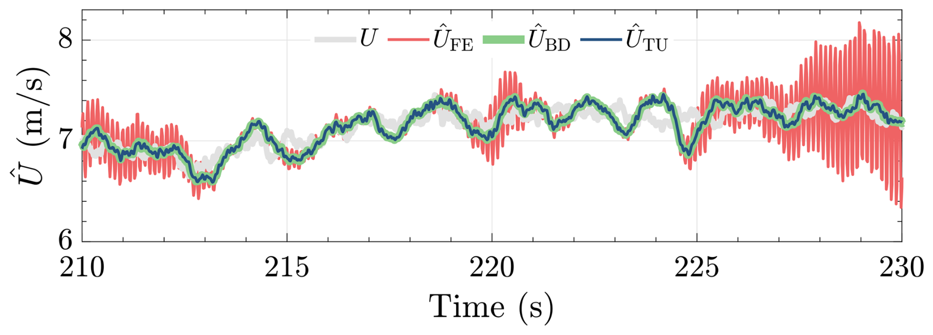
Figure 12 Actual wind speed U and wind speed estimates of the continuous wind speed estimate solver under different discretization methods ${\widehat{U}}_{(•)}$. The FE-discretized solver occasionally shows high-frequency oscillatory behavior, potentially due to combined nonlinearity and aliasing effects, which is not the case for that of the BD and TU methods for the chosen estimator gain κ=400.

Figure 13 depicts the time series comparison between the BD-discretized continuous solver and the iterative method. With the same tuning parameters as the previous simulation for the former, the latter is configured with i_max=5 and ${\mathit{ϵ}}_{\mathrm{U}}={\mathit{ϵ}}_{\mathrm{p}}=\mathrm{0.01}$, which are a good trade-off between accuracy and speed of the estimation. As evidently shown, both solvers demonstrate similar performance and accuracy for the presented case. However, in different scenarios, such as more noisy aerodynamic power and rotor speed estimates, both solvers may show disparities.

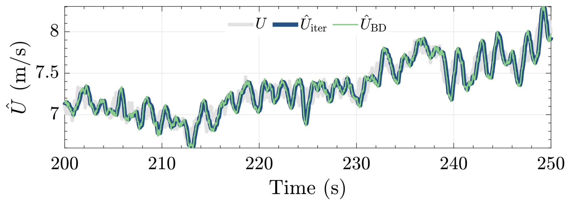
Figure 13 Actual wind speed U and wind speed estimates of the continuous and iterative single-step wind speed estimate solvers, the former of which is discretized with the BD method. Identical responses indicate that the accuracy of the wind speed estimate solvers depends, to a large extent, on the aerodynamic power (and rotor speed) estimation quality.

Noisy inputs would require the integrator gain of the continuous solver to be lowered such that high-frequency components in the input signals are attenuated but potentially result in lagged estimates. For the iterative solver, noisy inputs would increase the computational cost in terms of the higher number of iterations to converge to a solution.

Fortunately, as the roles of the aerodynamic power estimation (with a bonus of rotor speed filtering) and wind speed estimate solving are decoupled in this study, the task to ensure a low-noise and accurate wind speed estimate mostly relies upon the tuning of the former subcomponent. This way, few iterations and strict error tolerances of the iterative algorithm can be maintained. Such a condition also benefits the wind speed estimate of the continuous solver; however, as it requires a high gain to maintain good estimation quality, it is still prone to having the above-mentioned sampled-time system artifacts.

Hence, for the final and optimal design of the power balance wind speed estimation in this work, the combination of the state-estimation-based aerodynamic power estimator and iterative single-step wind speed solver is chosen and evaluated next in mid-fidelity simulations.

6 Mid-fidelity simulation setup and results

With the power balance wind speed estimation design finalized, this section covers the mid-fidelity validation of the proposed algorithm. The details of the simulation setup are covered in Sect. 6.1, and the validation results are discussed in Sect. 6.2. All code and data used to implement and validate the proposed wind speed estimation framework are openly available via Zenodo (Pamososuryo et al., 2024).

6.1 Simulation setup

The simulation setup for the mid-fidelity wind speed estimator validation in this work uses the open-source simulation code OpenFAST v3.5.3 (Jonkman et al., 2024), the development of which is led by the National Renewable Energy Laboratory (NREL). OpenFAST couples several nonlinear aero-hydro-servo-elastic computational modules by which realistic and complex wind turbine dynamic responses can be simulated with high accuracy. For the validation purposes of this work, the AeroDyn, ServoDyn, ElastoDyn, and InflowWind modules of OpenFAST are used. The BeamDyn module, capable of simulating blade structural dynamics, including blade torsion and bend-twist coupling, is not considered in this work; otherwise, higher-dimensional coefficient tables would have been necessary, as discussed in Lazzerini et al. (2024) (see also Remark 1). Future work will include the BeamDyn module, where higher-dimensional coefficient tables are required for validations.

Concerning the degrees of freedom (DOFs) of the simulated wind turbines, the following are activated:

• the generator

• the drivetrain rotational flexibility

• the first and second flapwise blade modes

• the first edgewise blade mode

• the first and second fore–aft tower modes

• the first and second side–side tower modes.

Note that the drivetrain rotational-flexibility DOF is turned off when a direct-drive wind turbine is simulated.

Two wind turbines representing the respective low- and high-power ratings are simulated, namely the NREL 5 MW and the IEA 22 MW turbines, as introduced in Sect. 2.2. In contrast to using the same C_p tables as in the previous analysis sections, using the reference wind turbine models in OpenFAST leads to simulating the aerodynamic properties of the respective turbines. The generator efficiency factors for both turbines are η_g=0.94 for the NREL 5 MW and η_g=0.954 for the IEA 22 MW.

With regard to the wind profile, Kaimal turbulent wind cases are considered for both turbines, with U_h=7.5 m s⁻¹ and $I_{\mathrm{T}}=\mathit{\{}\mathrm{4},\mathrm{12}\mathit{\}}\mathit{\%}$, generated using TurbSim (Jonkman, 2014), and used as input for the aforementioned InflowWind module. The simulations are run for 1060 s, in which the first 60 s is excluded to remove computational transients from the evaluation.

The power balance wind speed estimator employs the state-estimation-based method for the aerodynamic power estimation (Sect. 4), with its gain L computed using ω₀=5.75 rad s⁻¹ and ζ₀=4.5. Note that, compared to the initial low-fidelity simulations in Sect. 4.2.2, the lower frequencies and higher dampings of the estimator are chosen and considered to be a good compromise between noise filtering and good performance in the mid-fidelity settings. Better performance might be attained by the incorporation of more systematic tuning methods that are able to find the optimal gain via cost minimization (e.g., mean and variance of the wind speed estimate error), such as Bayesian optimization (Mulders et al., 2020) or genetic algorithms (Lara et al., 2024). With regard to the measurement noise, that of the rotor speed $v_{{\mathit{\omega }}_{\mathrm{r}}}$ is assumed to have a variance of ${\mathit{\sigma }}_{v_{{\mathit{\omega }}_{\mathrm{r}}}}^{\mathrm{2}}={\mathrm{10}}^{-\mathrm{5}}$ rad² s⁻², i.e., 1 order of magnitude higher than that used in the low-fidelity simulations in Sect. 4.3.

Constant- and tailored-gain settings are considered, the first one being computed using the LSS-equivalent inertia of the NREL 5 MW for both turbines, similar to what was done in Sect. 4.2.2, whereas the second one is tailored on the actual LSS-equivalent inertia of the simulated turbines (see Table 1). For the two turbines considered in this section, the chosen ω₀ and ζ₀ result in stable aerodynamic power estimators for both the constant- and the tailored-gain cases.

For the iterative single-step wind speed estimate solver, i_max=10 and ${\mathit{ϵ}}_{\mathrm{U}}={\mathit{ϵ}}_{\mathrm{p}}=\mathrm{0.005}$ are considered. Despite the tighter convergence bounds compared to the low-fidelity simulations in Sect. 5.2, the wind speed estimate in the simulations of this section only requires one iteration on average to solve.

The proposed method is also compared with an existing wind speed estimator, namely the Immersion and Invariance (I&I) REWS estimator, based on the work of Liu et al. (2022), a brief derivation of which is provided in Appendix A. This estimator is based on torque balance drivetrain dynamics, in which the internal model estimates the rotor speed and aims to minimize its difference from the actual measurements. Resultingly, the error compensation by a proportional-integral (PI) structure gives the wind speed estimate of this scheme. For both turbines in the low-turbulence scenario, the I&I estimator gains are K_p=15 m and K_i=3.5 m s⁻¹, whereas for the high-turbulence case, the gains are retuned to be K_p=25 m and K_i=5 m s⁻¹ to match the performance of the proposed method. Note that there have not been any studies yet in systematic tuning across a range of turbine sizes for the I&I approach, to the best of the authors' knowledge. Thus, the above PI gains are tuned heuristically and equally for the NREL 5 MW and IEA 22 MW. The next section covers the results from the OpenFAST simulations for the aforementioned settings.

6.2 Results

The time series performance evaluation of the power balance wind speed estimator is provided in this section for the considered reference turbines, the NREL 5 MW and IEA 22 MW. The statistical assessments of the numerical simulation results are provided at the end of this section.

Figure 14 depicts the time series results of the wind speed estimation for the NREL 5 MW. For both turbulent cases, it is shown that both methods are able to capture the slowly varying component of the actual wind speed well, with the proposed method showing less noisy results compared to I&I. This is mainly because the latter method, by default, does not contain any noise filtering feature, which can be added by low-pass filtering, for instance. Additional filtering would lead to additional phase lags and, thus, a slower wind speed estimation. The proposed estimator thus demonstrates superior noise handling capabilities over I&I, which obviates the need for additional filtering. However, as such a modification is not the main focus of this work, the original I&I structure is retained.

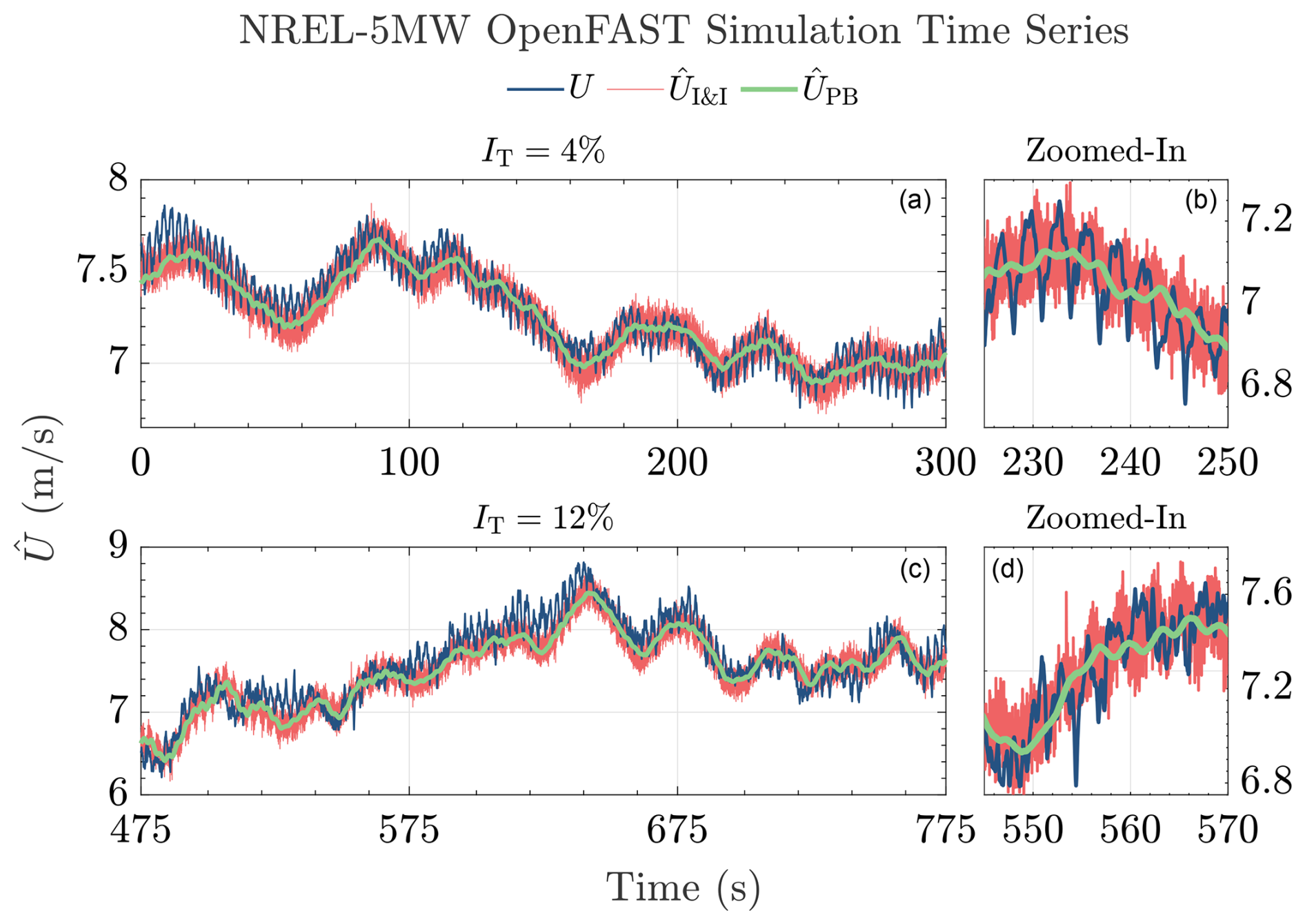
Figure 14 Wind speed estimation time series for the NREL 5 MW wind turbine. The proposed method (green line) gives a smooth, less noisy estimate compared to the I&I (red line) for low- (a, b) and high-turbulent (c, d) cases. The low-frequency component of the wind speed is captured where biased estimation occasionally occurs, potentially due to an inaccurate C_p table utilized in both estimators and an absence of dynamic inflow modeling in the estimators. The actual REWS, as outputted by OpenFAST, is shown by the blue line. Zoomed-in plots of 25 s time spans are provided on the right for clearer observation of the estimation performance.

An interesting behavior worth paying attention to in both wind speed estimation methods is the somewhat equal biases with respect to the actual wind speed. This is evident at the beginning of the low-turbulent wind case and at 525 and 625 s of the high-turbulent case. Such biases potentially come from the inaccuracy in the C_p table (Brandetti et al., 2022), which was generated by steady-state simulations, which might not necessarily be accurate during transients. Additionally, the absence of dynamic inflow effects in the estimator model could play a role in the appearance of such estimation biases (Knudsen and Bak, 2013).

Having presented the estimation results of the NREL 5 MW, those of the IEA 22 MW are now showcased. The main goal of the simulations with a larger turbine is to validate the performance differences between using constant and tailored estimator gains, with the proof of concept shown in the low-fidelity simulations in Sect. 4.2.2. Figure 15 depicts the time series results of the wind speed estimation for the IEA 22 MW wind turbine. For the constant-gain case, the L₂ aerodynamic power estimator gain is based on the L₂ gain tuned for the NREL 5 MW turbine, whereas that of the tailored-gain case is determined based on the inertia of the IEA 22 MW turbine using Eq. (22b). Evident in the figure is the better performance of the proposed method under tailored L₂ compared to under constant L₂ – note the displayed lagged behavior of the latter. With respect to the I&I results, the former performs similarly in terms of estimation quality of the low-frequency component in the wind speed with the advantage of less noisy estimates. Similar to the NREL 5 MW results previously, estimation biases are also observed in the IEA 22 MW case, which, again, are likely due to the inaccuracies in the C_p table of the corresponding turbine and absence of dynamic inflow modeling.

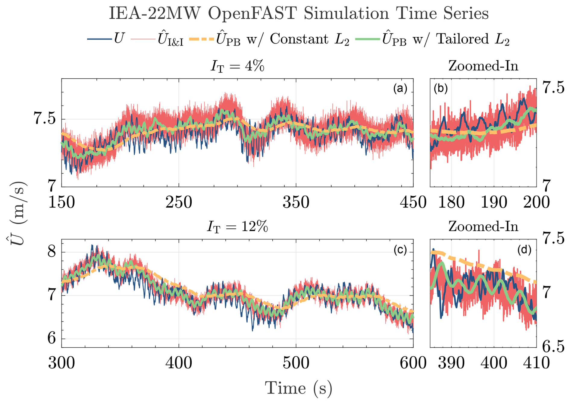
Figure 15 Wind speed estimation time series for the IEA 22 MW wind turbine. The proposed method gives a smooth, less noisy estimate compared to the I&I (red line) for low- (a, b) and high-turbulent (c, d) cases. Constant L₂ (dashed orange line) results in lagged estimation compared to gain-tailored L₂ (solid green line). The actual REWS, as outputted by OpenFAST, is shown by the blue line. Zoomed-in plots of 25 s time spans are provided on the right for clearer observation of the estimation performance.

From the aforementioned simulations, aerodynamic power and wind speed estimation error histograms are provided for the considered turbines. Figure 16 depicts the former, where the top row shows the histograms of the NREL 5 MW turbine and the bottom row the histograms of the IEA 22 MW. For all turbulent cases and estimators, the normalized aerodynamic power estimation errors, defined as $(P_{\mathrm{r}}-{\widehat{P}}_{\mathrm{r}})/P_{\mathrm{g},\mathrm{rated}}\cdot \mathrm{100}\mathit{\%}$, are shown to be similar. Most errors of the I&I and the proposed methods (only shown for the tailored-gain case) are concentrated at 0 %, with decreasing occurrences at larger percentages, resembling a bell curve. At higher turbulence intensity, wider histograms are obtained, which is logical due to the limitation of both estimators in capturing high-frequency contents of the actual REWS.

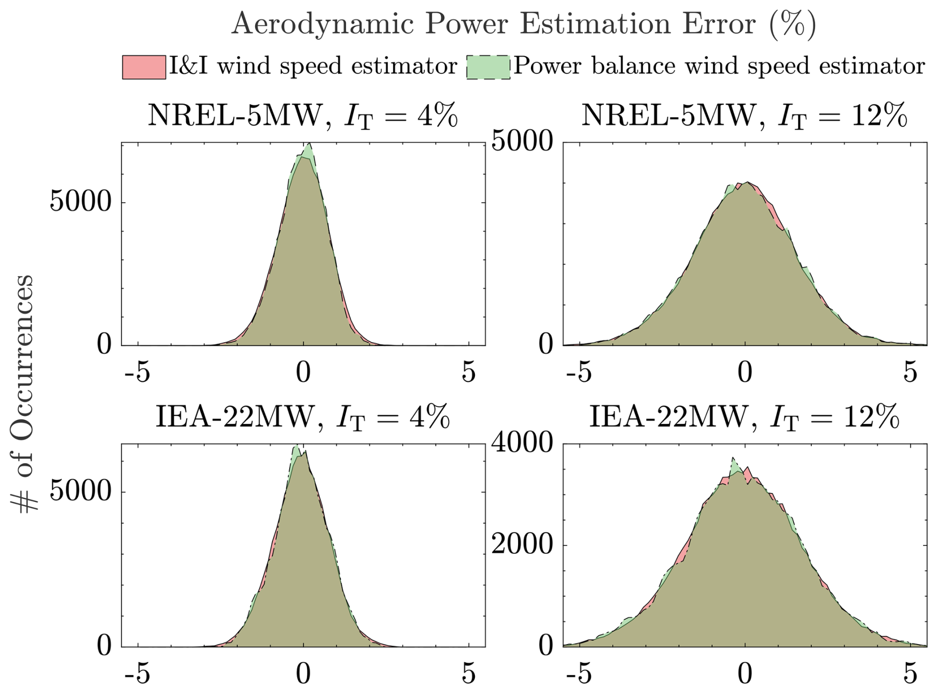
Figure 16 Aerodynamic power estimation error histograms of the wind speed estimators. Both the I&I and the proposed power balance wind speed estimator are shown to have similar aerodynamic power error distributions.

Figure 17 shows the histograms of the normalized wind speed estimation errors, defined as $(U-\widehat{U})/U_{\mathrm{h}}\cdot \mathrm{100}\mathit{\%}$. The figure sheds new light on the presence of skewed histograms. For the NREL 5 MW turbine, the error histograms are right-skewed, indicating the wind speed tends to be underestimated. On the contrary, the IEA 22 MW tends to be left-skewed; that is, the estimators tend to overestimate the wind speed value instead. Given that such skewness is not observed for the aerodynamic power estimation errors, the errors of the wind speed estimation might come from the inaccuracy of the C_p tables for the corresponding turbines, as previously suspected. Online calibration of such a C_p table has been studied, e.g., in Mulders et al. (2023a, b), which can be used to correct the wind speed estimation quality to minimize such skewness.

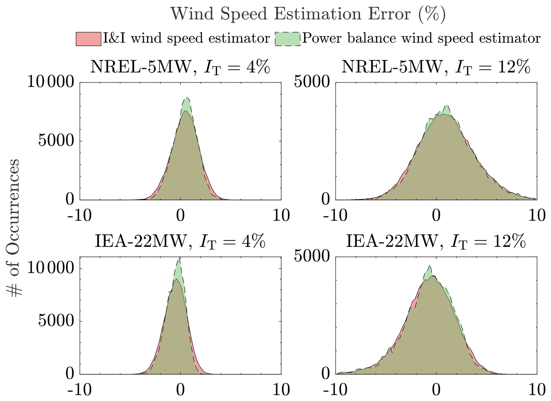
Figure 17 Wind speed estimation error histograms of the wind speed estimators. Both the I&I and the proposed power balance wind speed estimator are shown to have similar wind speed estimation error distributions. Subtle differences are also shown for both the I&I and the proposed power balance wind speed estimator, where the former has slightly higher occurrences at the histograms' tails due to the higher noise level, while the latter has slightly higher occurrences at the center of the distributions.

Based on the mid-fidelity simulation results reported above, the following conclusions of this section are drawn. First, it has been shown that the mean values of both the power-based wind speed estimator and the I&I are identical. Moreover, it has also been demonstrated that the use of steady-state information, i.e., through C_p tables, in a dynamic environment can lead to skewness for both estimators. Dynamic inflow modeling might also be required for future improvements to the current scheme. Nonetheless, under noisy measurement conditions, the former exhibits more noise resilience, whereas the latter requires additional filtering – complicating the design and potentially introducing phase lag. Finally, the convenience provided by the gain tailoring for the proposed method has allowed for performance calibration between the small and larger wind turbines.

7 Conclusions

In this work, an analysis framework and optimal design for a power balance REWS estimator have been proposed. The estimator is subdivided into two subcomponents based on their role in the scheme, namely, the aerodynamic power estimator and the wind speed estimate solver. Two aerodynamic power estimator techniques have been thoroughly analyzed, one based on the numerical derivative technique and the other based on the Luenberger state estimation technique. Of the two potential aerodynamic power estimators, the state-estimation-based technique has been chosen due to its better resilience against noisy measurements. Moreover, for the first time, a gain-tailoring method for performance calibration throughout a range of modern wind turbine sizes has been formalized. Regarding the wind speed estimate solvers, two options have also been considered, namely the continuous and iterative single-step solvers. In this study, the frequency-domain stability analysis of the former has been conducted in the continuous-time domain. Under the forward Euler discretization, deteriorations in the stability properties of this solver have been identified and shown in the discrete-time domain. Despite the favorable stability properties of the analyzed backward difference and Tustin discretization methods, the more robust iterative single-step wind speed estimate solver has been chosen and, in combination with the state-estimation-based aerodynamic power estimator, forms the optimal power balance wind speed estimator structure. This optimal power balance wind speed estimator has been validated in the mid-fidelity simulation environment OpenFAST, utilizing the NREL 5 MW and IEA 22 MW wind turbines, representing small and large wind turbines in the considered range, respectively. The proposed method and the considered “baseline” I&I wind speed estimator have shown similar performance in estimating the low-frequency component of the wind speed, with the latter having good REWS tracking, better noise resilience, and convenient estimator gain calibration across different turbine sizes.

Zero-bias aerodynamic power estimations have been obtained for both estimators; however, time series and histogram analyses have shown the appearance of biased wind speed estimations for both methods. Such biased estimations could be attributed to the inability of the steady-state C_p data used to estimate wind speed in a highly dynamic environment, excluding effects such as dynamic inflow. However, learning algorithms used to capture the true power coefficient during operation exist in the literature and can be incorporated to improve the performance of the proposed method.

A future study will consider providing an optimal means for tuning the estimator, e.g., through Bayesian optimization, incorporating currently unmodeled dynamics, such as drivetrain torsion, tower dynamics, and dynamic inflow effects, and accounting for blade pitch information.

Appendix A: Improved Immersion and Invariance wind speed estimator

The improved Immersion and Invariance (I&I) wind speed estimator, as studied in Liu et al. (2022), is described briefly in this section. Readers interested in the detailed derivations and analyses are referred to Liu et al. (2022).

The I&I estimator is described by the following torque balance equation:

$$\begin{array}{}\text{(A1)}& {\dot{\widehat{\mathit{\omega }}}}_{\mathrm{r}}\left(t\right)=\mathrm{\Phi }\left({\mathit{\omega }}_{\mathrm{r}}\left(t\right),\widehat{U}\left(t\right)\right)-{\displaystyle \frac{T_{\mathrm{g}}\left(t\right)}{J}},\end{array}$$

with the following nonlinearity:

$$\begin{array}{}\text{(A2)}& \mathrm{\Phi }\left({\mathit{\omega }}_{\mathrm{r}}\left(t\right),\widehat{U}\left(t\right)\right):={\displaystyle \frac{\mathit{\rho }A\widehat{U}(t{)}^{\mathrm{3}}{C}_{\mathrm{p}}\left(\widehat{\mathit{\lambda }}\left(t\right)\right)}{\mathrm{2}J{\mathit{\omega }}_{\mathrm{r}}\left(t\right)}}.\end{array}$$

The wind speed estimate is the result of the minimization of the error between rotor speed and its estimate by a proportional–integral compensator, that is

$$\begin{array}{}\text{(A3)}& \widehat{U}\left(t\right)=K_{\mathrm{p}}{e}_{{\mathit{\omega }}_{\mathrm{r}}-{\widehat{\mathit{\omega }}}_{\mathrm{r}}}\left(t\right)+K_{\mathrm{i}}\underset{\mathrm{0}}{\overset{t}{\int }}{e}_{{\mathit{\omega }}_{\mathrm{r}}-{\widehat{\mathit{\omega }}}_{\mathrm{r}}}\left(\mathit{\tau }\right)\mathrm{d}\mathit{\tau },\end{array}$$

with K_p as the proportional gain and K_i the integrator gain, where

$$\begin{array}{}\text{(A4)}& e_{{\mathit{\omega }}_{\mathrm{r}}-{\widehat{\mathit{\omega }}}_{\mathrm{r}}}\left(t\right)={\mathit{\omega }}_{\mathrm{r}}\left(t\right)-{\widehat{\mathit{\omega }}}_{\mathrm{r}}\left(t\right).\end{array}$$