Comparison of different simulation methods regarding loads, considering the centre of wind pressure

The centre of wind pressure (CoWP) (Schubert et al., 2025) introduces a concept to determine a flow structure from the incoming flow fields, which provides critical load information. This paper refines the approach in order to better understand how local flow structures affect the turbine. A new quantity, namely the load centre, is introduced to correlate the flow-related CoWP and the loads of the turbine. A novel calibration factor is introduced to establish a direct relationship between flow structures and aerodynamic loads. Therefore, simulations under laminar, shear, and turbulent inflow conditions are carried out, as well as with different wind turbine simulation methods. A good correlation between the turbulent inflow structures and loads from blade element momentum (BEM) simulations is found. High-resolution large-eddy simulations (LESs) even improve this correlation, attributable to the more resolved flow modelling capabilities.

1 Introduction

Installations of new, state-of-the-art wind turbines have to be carried out in accordance with current standards, e.g. the IEC61400-1 (IEC, 2019). The standards cover most aspects of turbines over their service life. This includes various operating points such as regular power generation, start-up phase, normal shutdown, and error handling. Some of these design load cases have to be tested under a whole range of wind speeds. In total, several hundred different cases have to be analysed for compliance with standards. Due to the enormous number of cases, it is necessary to use efficient tools that can deliver accurate results in the shortest possible time. Among these efficient tools is the centre of wind pressure (CoWP), introduced by Schubert et al. (2025), which characterises flow structures of the incoming flow field. This paper uses numerical simulations to validate the previous work.

In general, there are various techniques for simulating wind turbines. The most common are the blade element momentum theory (BEM), actuator line simulations (LES-ALs), and blade-resolved simulations (BLs). These methods differ significantly in terms of complexity and calculation effort. The simplest method is BEM, an engineering model in which the local velocities are estimated from an induction model and the resulting blade forces are calculated using lookup tables. Since simple surrogates of the flow field are used, BEM simulations are computationally efficient. LES-AL and BL are computational fluid dynamics (CFD) simulations in which the flow field around the turbine is calculated by solving the Navier–Stokes equations. Usually, a large-eddy simulation (LES) is used to model the turbulence. Thus, the impact of the turbulent inflow cases is not just treated by an induction factor. Still, the spatio-temporal development of the turbulent flow structures is resolved as they approach the turbine. On the one hand, LESs allow very accurate predictions of the interaction between the blades and the flow. On the other hand, LESs are orders of magnitude more costly than BEM. Accordingly, it would be impossible to simulate several hundred load cases for validation processes as part of the development and optimisation of wind turbines with computational capabilities. This is why BEM forms the basis of the development process.

This raises the following question: how accurate are the predictions using BEM compared to high-resolution LES? Due to the lack of flow modelling in the induction zone, a wind gust can disappear or be strongly deformed before it hits the rotor. The flow field immediately after the rotor can also affect the local blade aerodynamics. All of these phenomena can occur in reality and can be modelled with LES but cannot be represented in BEM. Hence, to evaluate such model uncertainties, comparative studies are of high interest. In particular, we focus on the issue of how local and temporal effects of flow structures (like the CoWP) can be captured for load investigations.

The following paragraph summarises existing comparisons from the literature. In Ehrich et al. (2018), the effects of turbulence on sectional forces are analysed for BEM, LES-AL, and BL. It was concluded that the time-averaged sectional forces for the centre section of the blade match between the simulation methods but differ at the blade root and tip. Liu et al. (2022) compared the power and thrust in BEM and LES-AL for laminar inflow. A comparison of the thrust coefficient for LES-AL and BEM in floating applications is carried out in Apsley and Stansby (2020). All these investigations lack a temporal comparison between the flow and the loads.

Nonetheless, whether or not these differences can be attributed to the modelling of the induction zone or the blade aerodynamics is not entirely clear. In this work, we address the question of how the general flow pattern of the inflow is influenced by the induction zone and how it affects the turbine loads. This includes a correlation analysis (flow to load) and an investigation of the influence of the induction zone on the turbulent fields, which is carried out for multiple flow scenarios.

Atmospheric turbulence is a crucial factor in regular energy production because wind fluctuations influence all aspects of the turbine. Consequently, turbulence modelling is a cornerstone of wind energy research (Veers et al., 2019; Kosović et al., 2025). The IEC standard specifies synthetic wind field models for emulating the effects of atmospheric turbulence. The Mann model (Mann, 1994, 1998) and the Kaimal model (Kaimal et al., 1972), as well as their parameterisations, are prescribed for this purpose.

As wind turbines are constantly being improved – i.e. reaching the physical limitations of the materials – the state-of-the-art development approach, based on BEM simulations, is reaching its limits. This is reflected in discrepancies between the simulated loads and the observed loads (Schubert et al., 2025). In principle, the origin of such differences may lie in the already-described issues in the simulation models or inaccuracies within the turbulence prescription. For efficient use of material and resources, as well as for ensuring the structural integrity of the turbines, it is necessary to determine the loads precisely. Therefore, improvements in both the turbulence description and the modelling assumptions are desirable.

There are various approaches to optimising turbulent fields. The recent work of Syed and Mann (2024a) and Syed and Mann (2024b) focuses on low-frequency, anisotropic wind fluctuations in the marine atmosphere. Syed and Mann (2024a) provide a model that extends turbulence spectra to $\approx \mathrm{1}{\mathrm{h}}^{-\mathrm{1}}$ by incorporating a two-dimensional formulation for large-scale fluctuations. In Syed and Mann (2024b), a Fourier-based method is presented to generate synthetic wind fields, combining the two-dimensional spectral tensor from Syed and Mann (2024a) for large structures and the uniform shear model from Mann (1994) for small-scale structures. In the works of Kleinhans (2008), Friedrich et al. (2022), and Yassin et al. (2023), the correct representation of small-scale structures in the inertial subrange is addressed. The velocity increments on the scale of a wind turbine and smaller are non-Gaussian distributed according to the K62 turbulence model. This property has been demonstrated for atmospheric turbulence in various works; see Mücke et al. (2011). However, this phenomenon is not considered by the models prescribed in the IEC standard.

The two previous strategies for improving turbulent fields are based on physically explainable gaps in the assumptions of the models currently in use. Schubert et al. (2025) have chosen a different, engineering-based approach. In their work, load measurements from a turbine are analysed regarding their damage equivalent load (DEL). It turns out that particular events, so-called bump events, which occur over timescales larger than 10 s, dominate the overall DEL. Interestingly, these large-scale events, identified in the time series of the loads, can also be found in the time series of a quantity calculated purely from the inflow wind field. Schubert et al. (2025) introduced this quantity as the centre of wind pressure (CoWP) to describe these large-scale events. This new characteristic quantity reduces the turbulent loads to a single point in the rotor plane. A pressure-induced yaw and tilt moment, i.e. bending moments at the main shaft of the turbine, can be calculated based on the CoWP location. The authors observed good agreement between the DEL from the introduced pressure-induced moments and the BEM-simulated moments.

Because these pressure-induced moments can be calculated exclusively from turbulence inflow data – independent of the wind turbine – load estimates can be obtained early in the development process. Building on this concept, Moreno et al. (2024, 2025) aim to describe the dynamics of the CoWP using stochastic models, particularly the Langevin approach.

This paper extends the investigation of the CoWP, already introduced in BEM Schubert et al. (2025), Moreno et al. (2024), and Moreno et al. (2025), by analysing the effect of the simulation method on the CoWP. To do this, three simulation approaches are compared: BEM, LES-AL, and BL with a delayed detached eddy simulation (DDES) for modelling turbulence. The simulation models are compared under different flow scenarios, ranging from laminar to turbulent cases, thereby generalising the previous studies. By comparing the various simulation models while simultaneously relating them with the flow, it can be shown that modelling the induction zone at LES-AL results in a better correlation with the loads than with BEM. Although the work of Moreno et al. (2025) quantitatively describes the relationship between the CoWP and wind turbine loads, it provides no one-to-one correspondence between inflow and aerodynamic response. This gap is closed in this work by introducing a calibration parameter that can be determined from a laminar simulation. The simulation settings for each approach and the selected flow scenarios are detailed in Sect. 3. Steady inflows are analysed in Sect. 4.1 and 4.2. The behaviour of the turbulence, including the CoWP, is analysed in Sect. 4.3.2. Subsequently, Sect. 4.3.3 shows how the CoWP affects a turbine in an LES.

2 Fundamentals

The following section explains specific aspects of the fields used in this work, namely turbulence and numerical models. For turbulence, these are synthetic turbulence (Sect. 2.1) and the centre of wind pressure (Sect. 2.2). The numerical models are BEM (Sect. 2.3) and CFD (Sect. 2.4) with the sub-model AL (Sect. 2.5).

2.1 Synthetic turbulence

The use of synthetically generated turbulence to mimic the influence of real atmospheric turbulence is a well-established procedure in research and is specified by the IEC standard (IEC, 2019; see Stoevesandt et al., 2022). The basic idea, as described by Veers (1984), was introduced to generate the fluctuations of atmospheric turbulence for numerical simulations efficiently and with low computational effort. The methodology works by describing the fluctuations in Fourier space according to a model spectrum of the kinetic energy. The spectrally modelled fluctuation tensor (e.g. in Eq. 1) is then converted into a three-dimensional field using inverse Fourier transformation. One of these models is the Mann model (Mann, 1994, 1998), which is proposed in the ICE standard and frequently used in research, which is why it is also used in this work. It implies the von Kármán spectrum (1948), and, consequently, the spectral tensor in wavenumber space (κ) follows

$$\begin{array}{}\text{(1)}& {\mathrm{\Phi }}_{ij}^{\text{iso}}\left(\mathit{\kappa }\right)={\displaystyle \frac{\mathit{\alpha }{\mathit{ϵ}}^{\mathrm{2}/\mathrm{3}}{L}^{\mathrm{17}/\mathrm{3}}}{\mathrm{4}\mathit{\pi }}}{\displaystyle \frac{{\mathit{\delta }}_{ij}{\mathit{\kappa }}^{\mathrm{2}}-{\mathit{\kappa }}_i{\mathit{\kappa }}_j}{[\mathrm{1}+(L\mathit{\kappa }{)}^{\mathrm{2}}{]}^{\mathrm{17}/\mathrm{6}}}}.\end{array}$$

The corresponding one-dimensional kinetic energy spectrum results in

$$\begin{array}{}\text{(2)}& F_i\left({\mathit{\kappa }}_x\right)=\left\{\begin{array}{ll}\frac{\mathrm{9}}{\mathrm{55}}\mathit{\alpha }{\mathit{ϵ}}^{\mathrm{2}/\mathrm{3}}\frac{\mathrm{1}}{{\left(L^{-\mathrm{2}}+{\mathit{\kappa }}_x^{\mathrm{2}}\right)}^{\mathrm{5}/\mathrm{6}}}& \text{for}i=x,\\ \frac{\mathrm{3}}{\mathrm{110}}\mathit{\alpha }{\mathit{ϵ}}^{\mathrm{2}/\mathrm{3}}\frac{\mathrm{3}{L}^{-\mathrm{2}}+\mathrm{8}{\mathit{\kappa }}_x^{\mathrm{2}}}{{\left(L^{-\mathrm{2}}+{\mathit{\kappa }}_x^{\mathrm{2}}\right)}^{\mathrm{11}/\mathrm{6}}}& \text{for}i=y,z.\end{array}\right.\end{array}$$

The resulting vector field exhibits a coherent field according to K41 theory (Kolmogorov, 1941). This means that the energy spectrum follows the $-\mathrm{5}/\mathrm{3}$ law, and the velocity increments are Gaussian distributed on all scales.

For parameterisation of the model, only three values are required: a length scale L to define the inertial subrange, a parameter for viscous dissipation $\mathit{\alpha }{\mathit{ϵ}}^{\mathrm{2}/\mathrm{3}}$, and a shear distortion parameter Γ that controls anisotropy by stretching the turbulent structures. In most cases, turbulence intensity (TI) is used for parameterisation instead of viscous dissipation as it is easier to measure and understand; see Larsen and Hansen (2007).

2.2 Centre of wind pressure

The centre of wind pressure (CoWP) introduced by Schubert et al. (2025) is a new characteristic quantity to describe flow structures and their influence on the loads of a wind turbine. The background to this was that certain load events (so-called “bump events”) identified from operating measured data could not be realistically reproduced or explained from numerical simulations using the turbulent fields from the given standards.

The CoWP is a measure used to grasp the spatial non-uniformity of the velocity field. It is described as the point in a velocity plane at which the total dynamic pressure from the velocity field acts. The formulation of Moreno et al. (2025) is used in this work. CoWP_i has two components, $i=[y,z]$, and is calculated from N discrete points in the velocity plane and their velocity in the main flow direction U_x:

$$\begin{array}{}\text{(3)}& {\text{CoWP}}_i\left(t\right)={\displaystyle \frac{{\sum }_{k=\mathrm{1}}^N{i}_k\cdot U_x^{\mathrm{2}}(y_k,z_k,t)}{{\sum }_{k=\mathrm{1}}^N{U}_x^{\mathrm{2}}(y_k,z_k,t)}}.\end{array}$$

For a turbulent wind field, the CoWP is therefore a time-dependent coordinate in a plane parallel to the rotor surface, which can be determined from synthetic data or measurements. Figure 1 shows the time series of the two components, Y and Z, of the CoWP from a synthetic wind field in (a) and (b). Two particular times are marked by the red and green dots. Those correspond to the global maximum and minimum of CoWP_Z. The instantaneous velocity planes of the wind field at those two times t=250 and t=588 s are shown in (c) and (d). The location of the CoWP and the centre of the section are marked by the red and green dots and the black crosses, respectively. The location of CoWP_Z can be explained in the velocity planes by the presence of regions with higher velocities in the upper and lower ranges, respectively. At this point, it should be briefly noted that the CoWP is relatively close to the centre of the rotor plane, with amplitudes of approx. 3 m. Due to the high thrust, this offset still results in considerable bending moments on the main shaft.

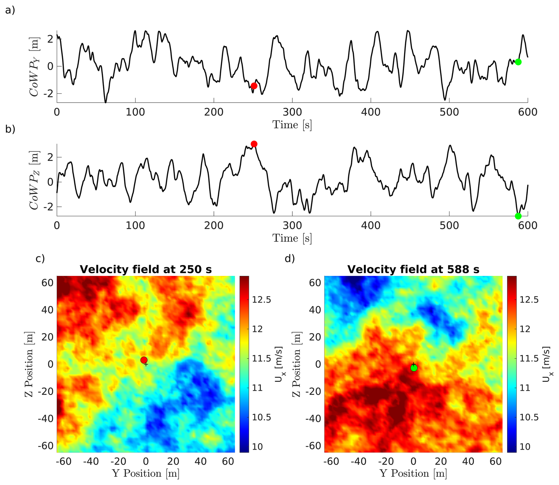
Figure 1 Time series of CoWP_Y in (a) and CoWP_Z in (b) from the synthetic wind field used in this work. Velocity slices of the wind field corresponding to the CoWP_Z maxima in (c) and minima in (d). The CoWP locations are shown by the red and green dots in the time series and the velocity slices. The centre of the slice is shown by the black cross.

In the work by Moreno et al. (2025), a characterisation of the dynamics of the CoWP is carried out based on the statistical properties of the signals. The Langevin approach (Friedrich and Peinke, 1997) is used for this characterisation by calculating the drift and diffusion values of the system. Because of the strong correlation to the bending moments at the main shaft, the dynamics of the CoWP are used to reconstruct random signals of the moments. Their work shows that the combination of the CoWP and the Langevin approach allows for an estimation of the loads without a simulation or even a wind field, as the loads are determined from a stochastic process. The main advantage of the stochastic reconstruction is that very long time series can be generated efficiently, which is essential for the assessment of the loads over the lifetime of the turbine.

2.3 Blade element momentum theory

BEM theory is a fundamental analytical tool used to predict the aerodynamic performance of propellers and wind turbines. It integrates two concepts: blade element theory (Froude, 1878), which examines the forces on individual blade sections, and momentum theory (Rankine, 1865), which considers the conservation of linear and angular momentum in the flow through the rotor plane.

In BEM theory, the rotor blade is divided into numerous small elements along its length, which are assumed to be independent of each other. The local relative velocity and the angle of attack are calculated for each element based on the rotational speed and the turbulent inflow. The local lift and drag forces are determined from lookup tables for the airfoil sections. These aerodynamic forces are then used to compute the contributions to thrust and torque from each blade segment. In parallel, momentum theory is applied to account for the induced velocities in the axial and tangential directions resulting from the energy extracted by the rotor.

Since the Navier–Stokes equations are not solved in a discretised flow domain, BEM simulations are fast and widely used. At the same time, this constitutes the major drawback of BEM, since it can lead to substantial deviations from reality. For the accurate modelling of complex flow phenomena near the blade tip and the blade root in particular, as well as for unsteady aerodynamics such as dynamic stall, the differences to measurements or high-resolution models are notable. To address these issues, different models exist to correct the initial calculation; see Glauert (1935).

2.4 Computational fluid dynamics

In CFD, the Navier–Stokes equations are used to simulate fluids. For incompressible flows, these are

$$\begin{array}{}\text{(4)}& {\displaystyle }& {\displaystyle }\mathrm{\nabla }\cdot \mathit{U}=\mathrm{0},\text{(5)}& {\displaystyle }& {\displaystyle \frac{\partial \mathit{U}}{\partial t}}+(\mathit{U}\cdot \mathrm{\nabla })\mathit{U}=-\mathrm{\nabla }p+\mathrm{\nabla }\cdot \left(\mathit{\nu }\mathrm{\nabla }\mathit{U}\right)+\mathit{F},\end{array}$$

where U is the velocity vector, p is the kinematic pressure, and ν is the kinematic viscosity. F is the source term with which external forces, such as gravity, can be applied to the fluid. As proposed by Spille-Kohoff and Kaltenbach (2001) and Gilling and Sørensen (2011), this source term can also be used for a turbulent inflow inside the domain. For this purpose, the fluctuations from the wind field u_i,turb are considered to be accelerations of the background velocity, which is then converted into the following force:

$$\begin{array}{}\text{(6)}& F_{i,c}={\displaystyle \frac{\mathrm{1}}{\mathrm{2}}}{A}_c\left(U+{\displaystyle \frac{\mathrm{1}}{\mathrm{2}}}{u}_{i,\text{turb}}\right)u_{i,\text{turb}}.\end{array}$$

2.5 Blade-resolved and actuator line wind turbine representation

The most obvious representation of a wind turbine in CFD is blade resolved (DDES-BL). For this, the exact geometry of the wind turbine is resolved by the numerical grid. This requires a large number of small cells around the blades in order to be able to capture all aerodynamic effects. Due to the small cells, a small time step is required for the simulation as well. The combination of many cells and a small time step makes blade-resolved simulations computationally intensive.

The actuator line method (LES-AL) introduced by Sørensen and Kock (1995) is a computational technique used in CFD to simulate wind turbine aerodynamics efficiently. Instead of modelling the full geometric complexity of turbine blades, LES-AL represents each blade as a line of discrete force elements distributed along its span. These elements apply forces to the flow field through the source terms F in Eq. (5), replicating the aerodynamic effects of the blades without the need for detailed geometric resolution.

In LES-AL, the forces are calculated based on local flow conditions from the CFD field and airfoil characteristics from lookup tables. The force determination for the LES-AL is based on the same lookup tables as for BEM methods. To mitigate singularities and numerical instabilities, the body force vector is distributed over the flow field using a Gaussian function as introduced by Sorensen and Shen (2002).

This approach allows for the capture of essential aerodynamic interactions between the turbine and the surrounding flow field, including wake formation and evolution, while significantly reducing computational costs compared to fully resolved LES-BL simulations by modelling the actual airfoil flow interaction.

2.6 Comparison of the different methods

When developing a new wind turbine, various tools for load prediction are available. They differ in model complexity and, consequently, in the computational effort required to simulate a specific load case. The crucial question is what level of detail is required for the load prediction for the specific components of a wind turbine.

Table 1 shows a comparison of various existing tools for load prediction. BEM, LES-AL, and DDES-BL are frequently used and well established in research. Their respective advantages and disadvantages are commonly known and well documented. The newly introduced CoWP differs from previously described models, as it has so far been presented exclusively using BEM simulations. Therefore, it remains unclear whether the concept can also be generalised for high-resolution LESs. Furthermore, the signals are normalised in both papers, and it remains to be clarified how CoWP can be converted into a load signal.

Table 1 Overview of different load prediction tools.

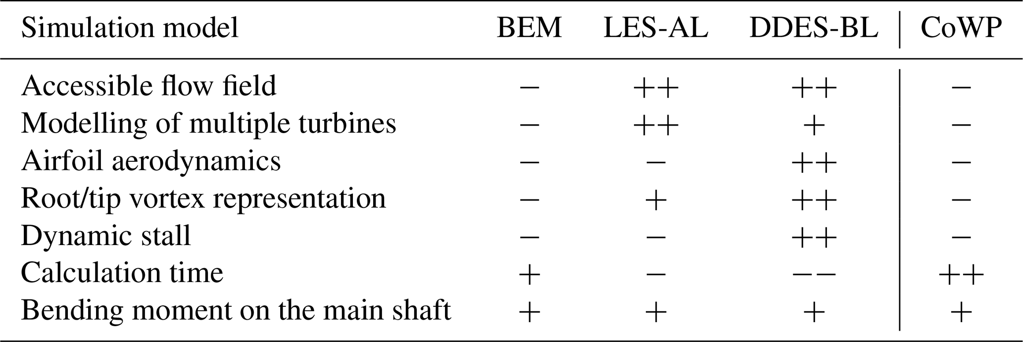
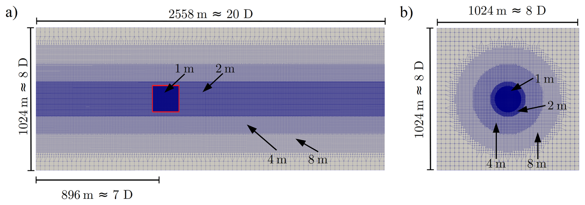
Figure 2 Cutting slices of the grid used for the CFD simulations normal to the rotor area in (a) and parallel to the rotor area in (b). The different refinement regions and the respective cell size are displayed in the figure. The turbine is placed in the red square with the finest cells.

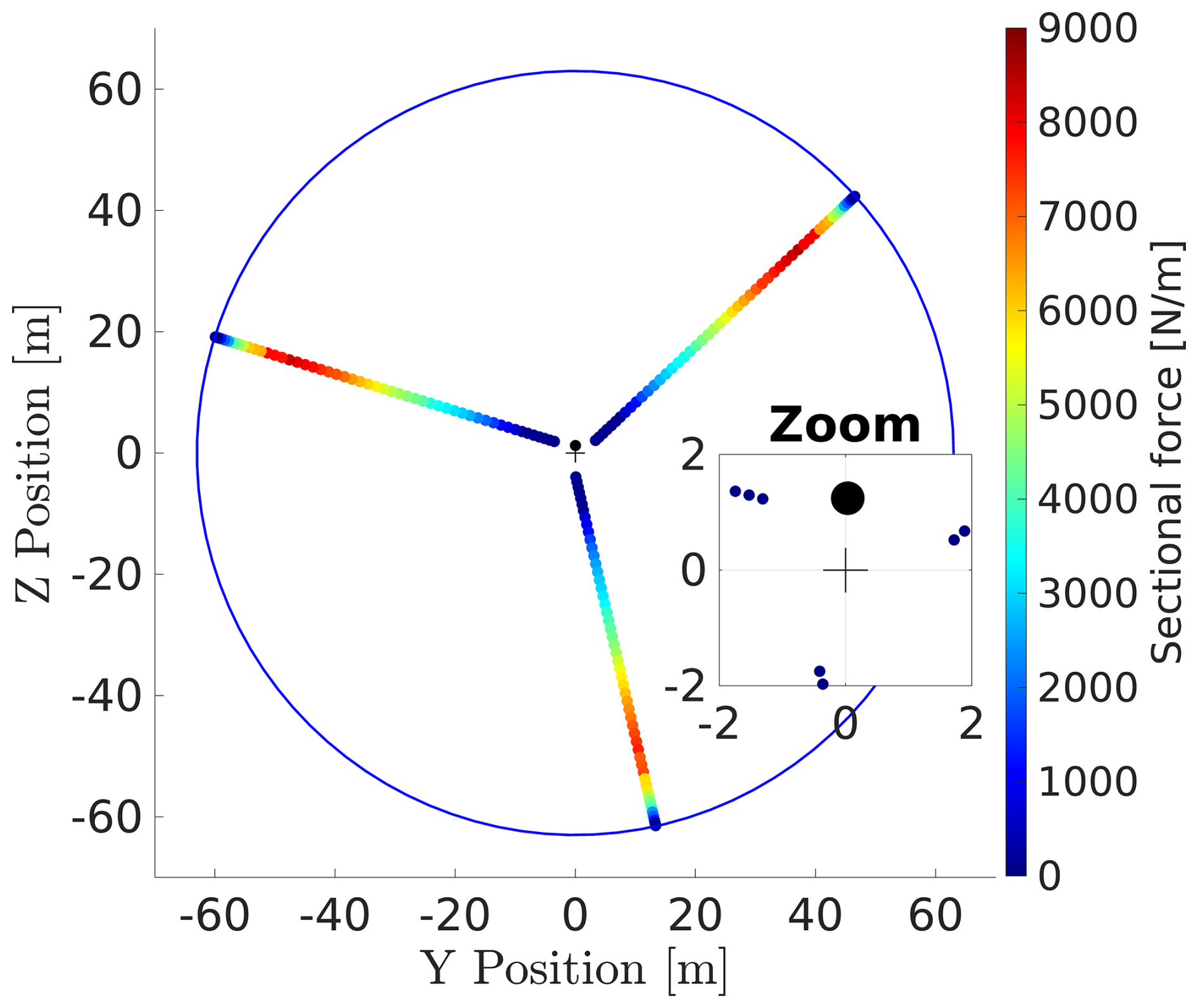
Figure 3 Force array for the load centre estimation of an LES-AL simulation, showing the sectional forces. The centre of the rotor is shown by the black cross, and the rotor area is marked by the blue line. The big black dot shows the load centre. A close-up has been added to improve the display of the CoWP position in relation to the centre point.

3 Methodology

Here, a detailed presentation of the numerical setup is given. It starts with the selected turbine and the operating point (Sect. 3.1), followed by parameterisation for the BEM simulation (Sect. 3.2) and the CFD simulation (Sect. 3.3) in terms of the solver, the grid, the numerical schemes, and the turbulence models. It ends with a physical derivation of the load centre (Sect. 3.5) and a description of the selected flow scenarios (Sect. 3.6).

3.1 Turbine setting

The investigation in this work is carried out with the NREL 5 MW reference turbine (Jonkman, 2009) with a diameter of 126 m. This model turbine is commonly used for scientific studies. To neglect all periodic loads, a very simplified rotor is represented; i.e. the rotor is not tilted, the blade has no cone angle, and the pitch angle is constant. Additionally, there is no tower (similar to Dose et al., 2018). The turbine is operated in rated conditions ($U_x=\mathrm{11.4}\mathrm{m}{\mathrm{s}}^{-\mathrm{1}}$), with a constant rotor speed of 12.1 rpm.

3.2 BEM setup

The BEM simulations are performed with the open-source tool OpenFAST v2.5 with the provided repository for the NREL 5 MW reference turbine (Jonkman et al., 2021). The controller, gravity, ground effect, tower effects, and dynamic stall model are turned off to model the same setup as in CFD. The blade pitch angle and the rotational speed are defined as constant, with values of 0° and 12.1 rpm, respectively.

3.3 CFD setup

The CFD simulation is carried out with the open-source toolbox OpenFOAM v2306 (OpenCFD, 2023). The incompressible unsteady solver pimpleFOAM (Greenshields and Weller, 2022) is used, which uses a combination of the PISO (Issa, 1986) and SIMPLE (Patankar and Spalding, 1983) algorithms for pressure–velocity coupling. A second-order backward scheme is used for the time derivative, and a second-order linear upwind scheme is used for the convective term.

The turbulence is modelled with the standard Smagorinsky (Smagorinsky, 1963) subgrid-scale model for the LES-AL case. For the DDES-BL case, a delayed detached eddy simulation is used (Gritskevich et al., 2012). This is a hybrid between the k–omega SST model (Menter et al., 2003) near the wall and a standard Smagorinsky model (Smagorinsky, 1963) for the far field. This ensures that the flow in the induction zone is computed using the same subgrid models.

3.3.1 Mesh settings

The same base mesh is used for all LESs (LES-AL and DDES-BL for the three flow scenarios), which is shown in Fig. 2. For the DDES-BL simulations, there is an additional rotor region with the blade meshes and the hub. The simulation domain has a length of 2558 m (≈20 D) and a width/height of 1024 m (≈8 D). In the base mesh, all cells are quads with an aspect ratio of 1. In the area of the rotor, as well as the direct near wake, the cells have a resolution of 1 m. Over the entire length of the domain, there is a cylindrical refinement zone with a diameter of 240 m (≈2 D) and a resolution of 2 m. Further outwards, the cells become coarser in other refinement zones, resulting in a total cell count of 27.2 million cells. A grid study is attached in Appendix A.

Table 2 Overview of the different location quantities.

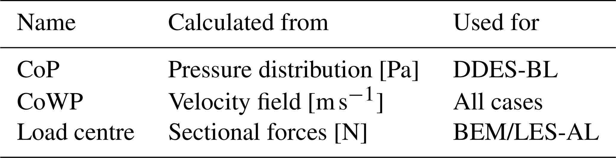
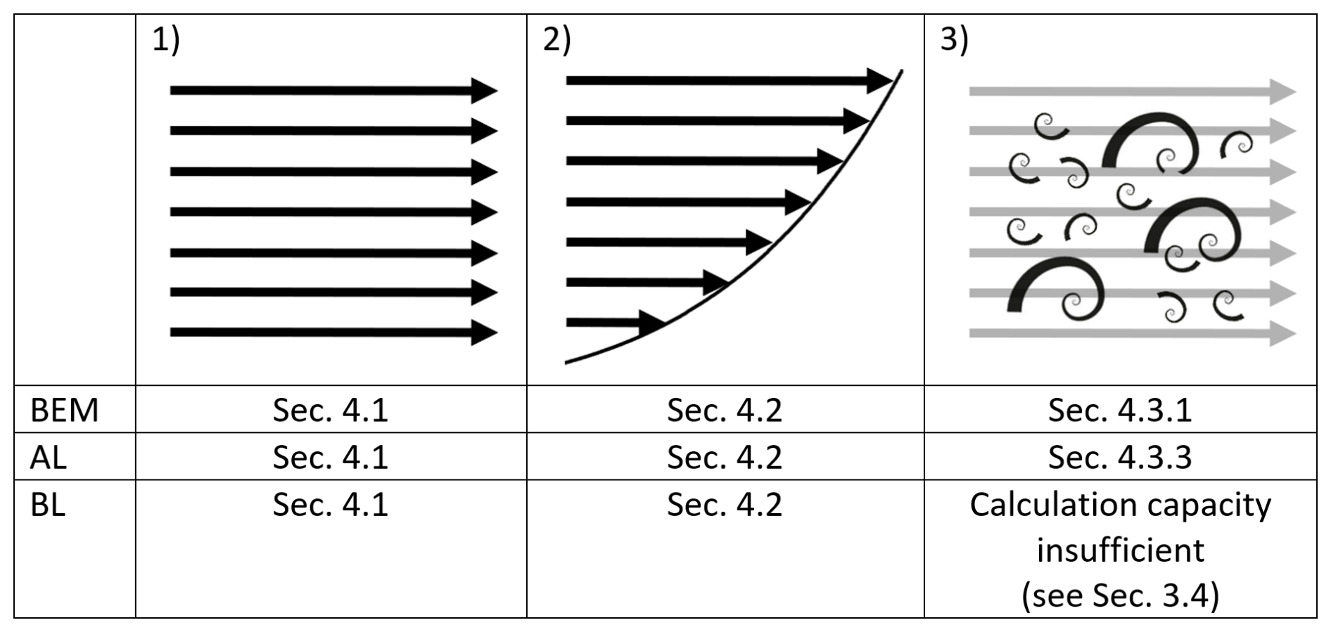
Figure 4 Schematic illustration of the flow scenarios. (1) Uniform laminar, (2) laminar shear flow, and (3) turbulent. Additionally, the corresponding sections are shown below the pictures.

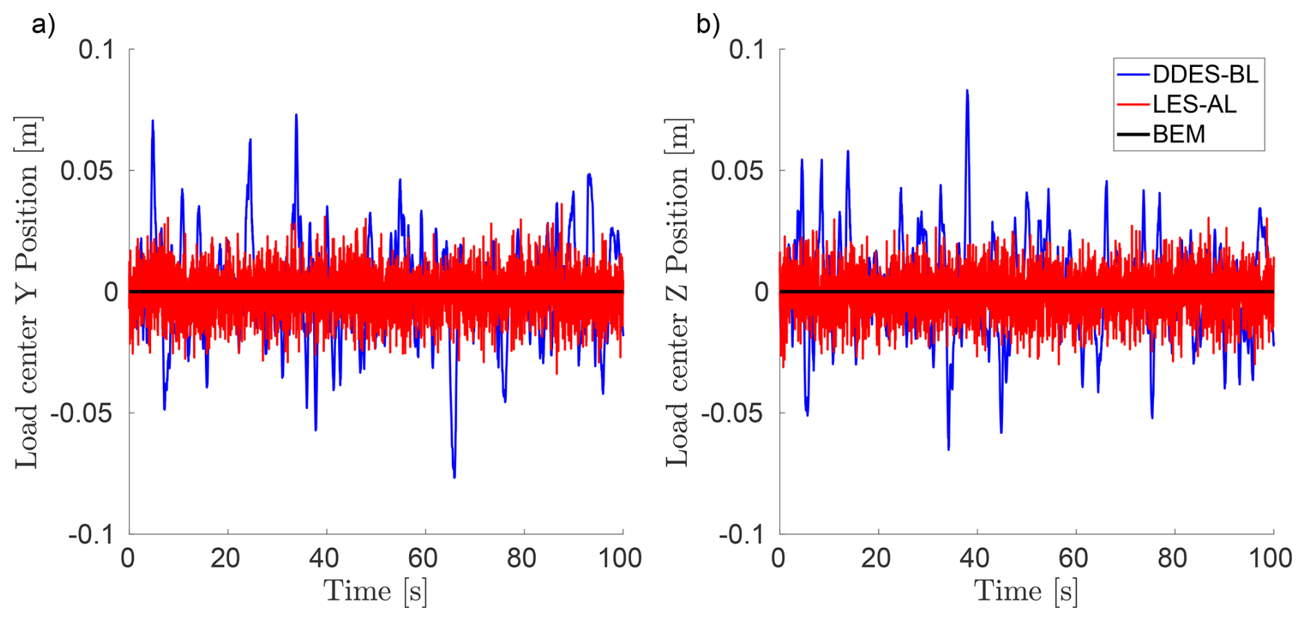
Figure 5 Time series of the load centre for the three simulation methods with laminar inflow. Y component in (a) and Z component in (b).

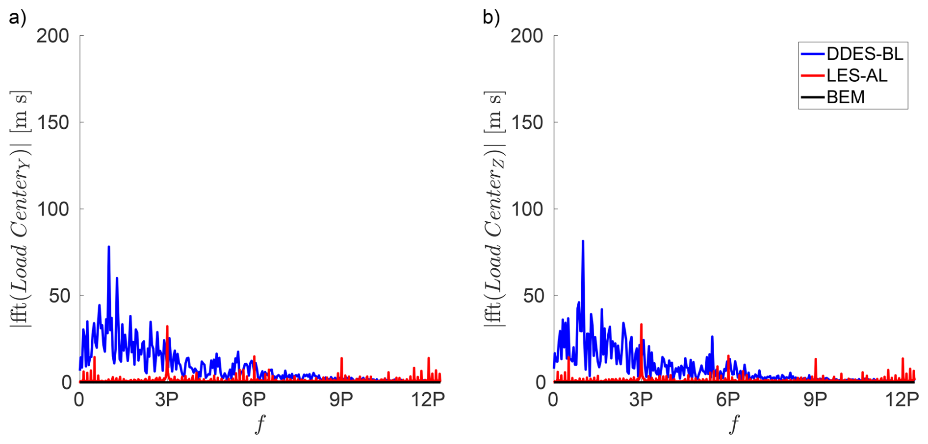
Figure 6 FFT of the load centres for the three simulation methods for the uniform laminar case. Y component in (a) and Z component in (b) (3 P=0.605 Hz).

3.3.2 Actuator line model

The actuator line implementation in OpenFOAM used in this work employs the version by Bachant et al. (2016, 2024). In this implementation, the required airfoil lookup tables for the 5 MW reference turbine are provided in tutorials. The turbine is set up without a tower by commenting out this section. To model the tip and root losses, the Glauert model (Glauert, 1935) is used. Along the span, 57 points per blade are used. To extract the sectional forces, both the blade performance and the element performance options are enabled.

3.3.3 Blade-resolved settings

The blade mesh is created with the in-house blade meshing tool, blade block mesher (Schmidt et al., 2012). In this grid generation tool, several structured two-dimensional airfoil sections are connected along the span. The blade mesh of this paper is the same as in the work of Dose et al. (2018) and Höning et al. (2024). It is a C-mesh topology with a resolution of 300 cells chordwise and 40 cells normal to the wall, with a growth ratio of 1.2. Along the span resolution, 260 cells are used, totalling 3.56 million cells per blade. The first cell resolution is chosen for a high-Re approach with wall functions, where the majority of the cells are within $\mathrm{30}<y+<\mathrm{70}$. The base mesh with blade and rotor mesh combined has a total of 44.6 million cells.

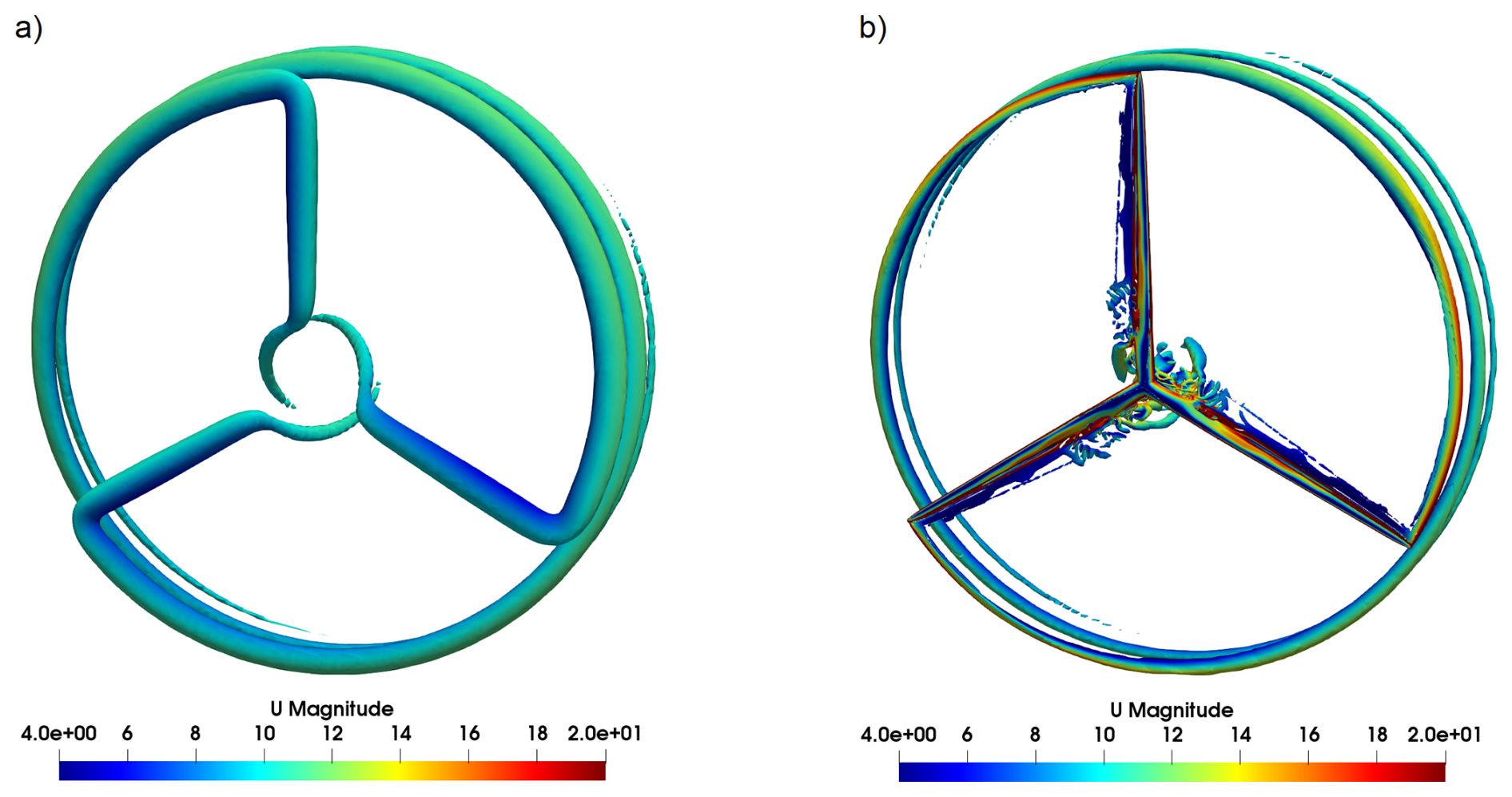
Figure 7 Isosurfaces of the Q criterion for (a) the LES-AL ($Q=\mathrm{0.2}{\mathrm{s}}^{-\mathrm{2}}$) and (b) the DDES-BL ($Q=\mathrm{1.2}{\mathrm{s}}^{-\mathrm{2}}$) visualised with the flow velocity for the uniform laminar case.

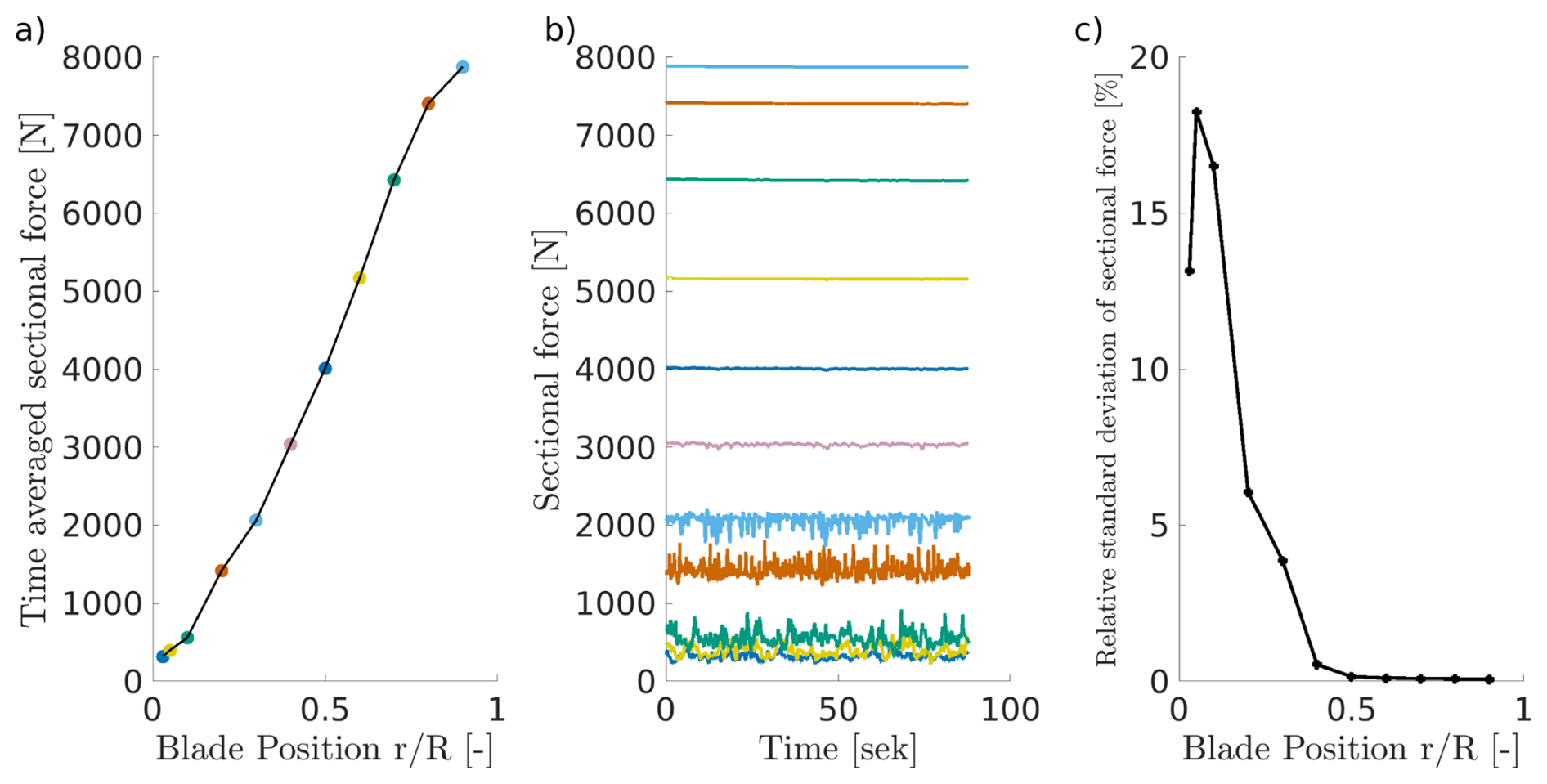
Figure 8 Sectional forces of a blade-resolved simulation with laminar inflow. Time-averaged sectional forces over blade radius (a). Time series of the sectional forces (b). Relative standard deviation of the sectional forces over blade radius (c).

3.4 Calculation time

The varying complexity of the different models results in a significantly different calculation effort. The BEM simulations are carried out on a local workstation. A case of 200 s simulation time takes approximately 75 s (wall time). In other words, to simulate 1 s with one processor, 2.67 CPUs are required (wall time divided by number of processors; assuming BEM runs serial). For an LES-AL simulation, this corresponds to 45 000 CPUs per second (parallel on 128 cores), and for a DDES-BL simulation, it corresponds to 1 500 000 CPUs per second (parallel on 256 cores). To summarise, this means that an LES-AL simulation is 16 800 times more costly than BEM, and a DDES-BL simulation is 561 000 times more expensive than BEM.

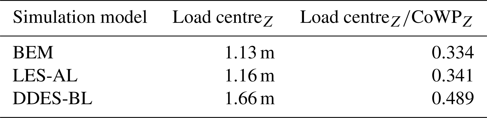
Table 3 Load centre and calibration factor for the laminar shear case.

3.5 Centre of pressure and load centre

In order to explain the methodology used in this paper in detail, we briefly repeat the centre of pressure (CoP). This is a well-known and established concept in fluid dynamics; see Anderson (2016). It is the location from which a point force has the same effect on an object as the pressure forces acting on the surface. The CoP location is often used to describe the stability of sailing boats, aircraft, or cars. It is calculated by setting up a matrix equation with the aerodynamic forces F_aero and aerodynamic moments M_aero and solving for the CoP:

$$\begin{array}{}\text{(7)}& {\mathit{F}}_{\text{aero}}\times \mathrm{CoP}-{\mathit{M}}_{\text{aero}}=\mathrm{0}.\end{array}$$

In our case, this makes the CoP a turbine-specific variable that is calculated from the pressure distribution in response to the flow around the turbine.

Schubert et al. (2025) apply the idea of the CoP to a flow field by replacing pressure with the velocity squared. This makes the CoWP a pure flow quantity that is independent of any object.

The load center is introduced now, with the same motivation as the CoWP. As there is no resolved geometry in the BEM and LES-AL models, the CoP cannot be calculated. Instead, there are sectional forces of the blade segments. For a given time step of a BEM or LES-AL simulation, the location of each blade segment and the corresponding thrust force F_x are known. Instead of a velocity plane at the CoWP, a sparsely filled plane with the thrust forces is used for the load centre calculation (shown in Fig. 3). The load centre is then calculated in the same way as the CoWP.

$$\begin{array}{}\text{(8)}& {\text{Load centre}}_k\left(t\right)={\displaystyle \frac{{\sum }_{i=\mathrm{1}}^N{k}_i\cdot F_x^{\mathrm{2}}(y_i,z_i,t)}{{\sum }_{i=\mathrm{1}}^N{F}_x^{\mathrm{2}}(y_i,z_i,t)}}\end{array}$$

In summary, there are three quantities with the unit metre, all of which represent a distance from the rotor centre. Therefore, these quantities are ideally suited for comparison with each other. To clearly distinguish between them, the differences are briefly outlined here once again: due to the simplifications in the blade element theory on which BEM and AL are based on, an analogy can be drawn between the CoWP (Fig. 1c) and the forces of the blade elements (Fig. 3) (Eqs. 3 and 8, respectively).

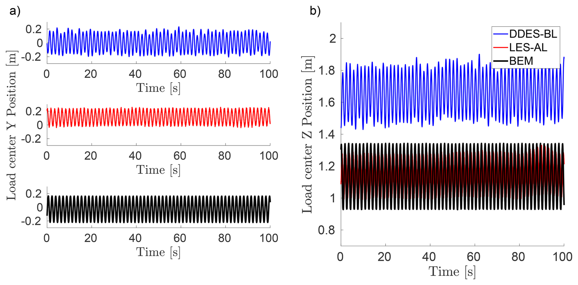
Figure 9 Time series of the load centre for the three simulation methods with shear flow. Y component in (a) and Z component in (b).

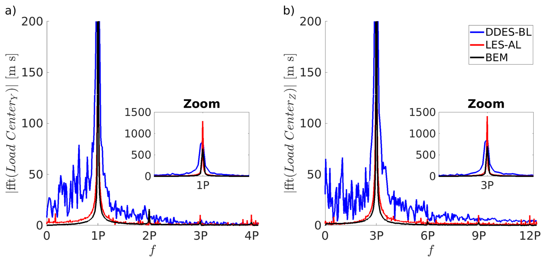
Figure 10 FFT of the load centres for the three simulation methods with shear inflow. Y component in (a) and Z component in (b) (3 P=0.605 Hz).

In blade-resolved simulations, there are no simplified blade elements but rather a fully represented pressure distribution of the blades. From this pressure distribution, the CoP can be calculated, which causes bending moments on the main shaft. However, the CoP additionally includes the force component responsible for rotation. Due to the complex three-dimensional geometry of the blades, it is not possible to calculate the load centre. Within this work, the component of the CoP responsible for rotation is not evaluated. Nevertheless, for the sake of simplicity, this paper always refers to the load centre when referring to loads. A summary of the given quantities can be found in Table 2.

3.6 Flow scenarios

Three flow scenarios are investigated (see Fig. 4):

1. A uniform laminar flow is used as proof of concept and to determine the basic uncertainty in the models.

2. A laminar shear flow is employed to determine the differences between the methods and how the shear profile interacts with the turbine. A power law profile with an exponent of α_shear=0.143 is used, which is a typical value for an offshore location (Hsu et al., 1994). The hub height of the turbine is used as the reference height.

3. A turbulent flow is used to determine a realistic case. The Mann model is used to generate the turbulent wind field (see Sect. 2.1). The field is parameterised by L=126 m (=1 D) and TI=5 %. To simplify the analysis, no shear is used (Γ=0), as the Taylor hypothesis for frozen turbulence (Taylor, 1938) can thus be applied. The field should have a resolution of 2 m in each spatial direction to be consistent with the recommendation of Troldborg et al. (2014). Furthermore, the wind field should fill the entire LES domain and enable a simulation of 10 min – the usual investigation interval in the wind energy field. The average speed and spatial resolution result in a temporal resolution of 0.175 s. The required wind field must therefore have dimensions of $\mathrm{6860}\mathrm{m}\times \mathrm{1024}\mathrm{m}\times \mathrm{1024}\mathrm{m}$ ($\mathrm{3430}\mathrm{points}\times \mathrm{512}\mathrm{points}\times \mathrm{512}\mathrm{points}$). To create such a field with ≈900 million points the turbulence generator introduced by Liew et al. (2023) and Liew (2022) is used.

4 Results and discussion

In the following section, the results are presented in the order of the flow scenarios from Sect. 3.6, starting with the laminar flow in Sect. 4.1. The shear flow and the calibration factor are presented in Sect. 4.2. The turbulent inflow with BEM is then shown in Sect. 4.3.1. The turbulent characterisation in an empty box is done in Sect. 4.3.2. Finally, the turbulent LES-AL case is presented in Sect. 4.3.3.

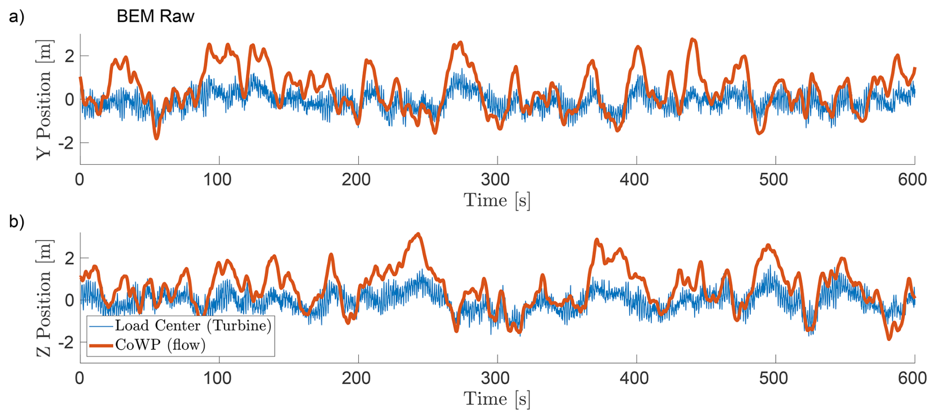
Figure 11 Direct comparison of the time series of the CoWP from the synthetic inflow field (orange) and the load centre (blue) of the BEM simulation. Y component in (a) and Z component in (b).

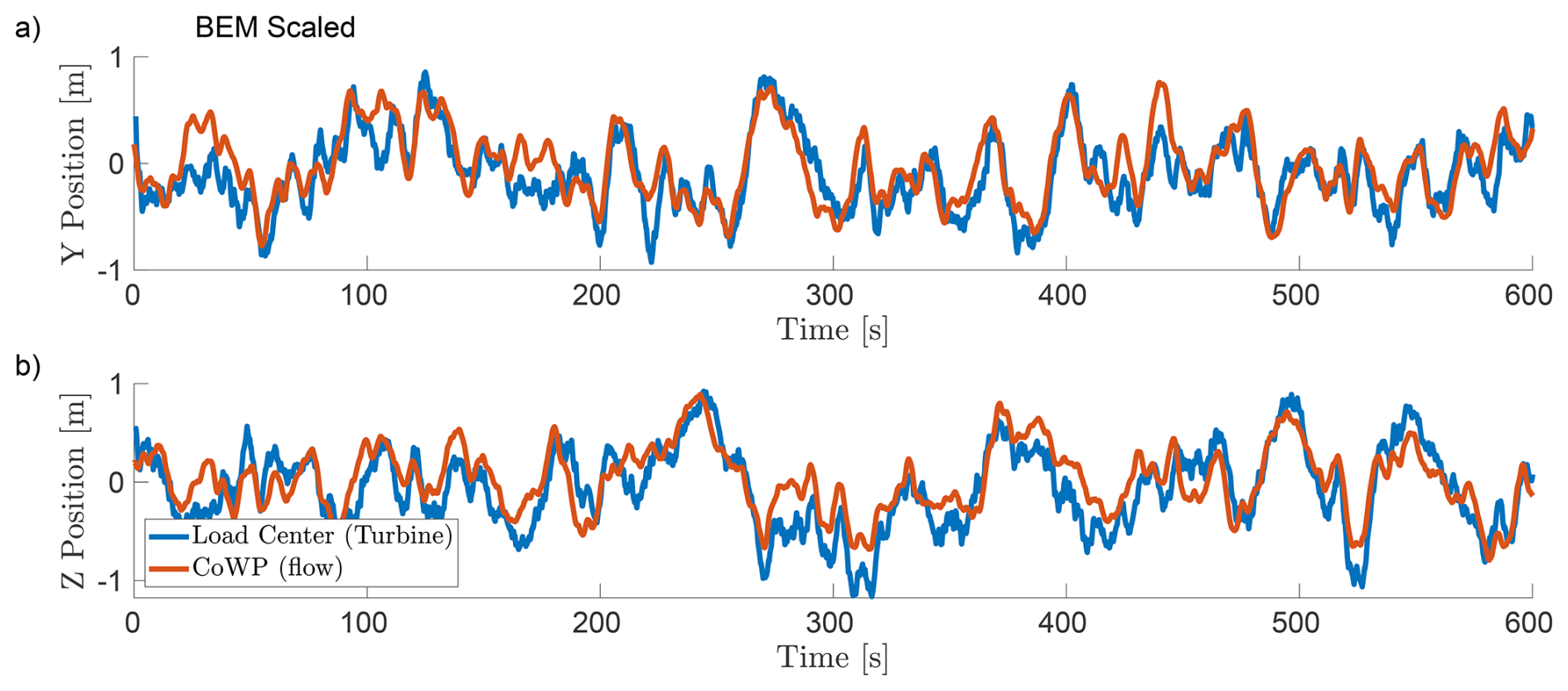
Figure 12 Direct comparison of the time series of the scaled CoWP from the synthetic inflow field (orange) and the filtered load centre of the BEM simulation (blue). Y component in (a) and Z component in (b). r_Pearson=0.814.

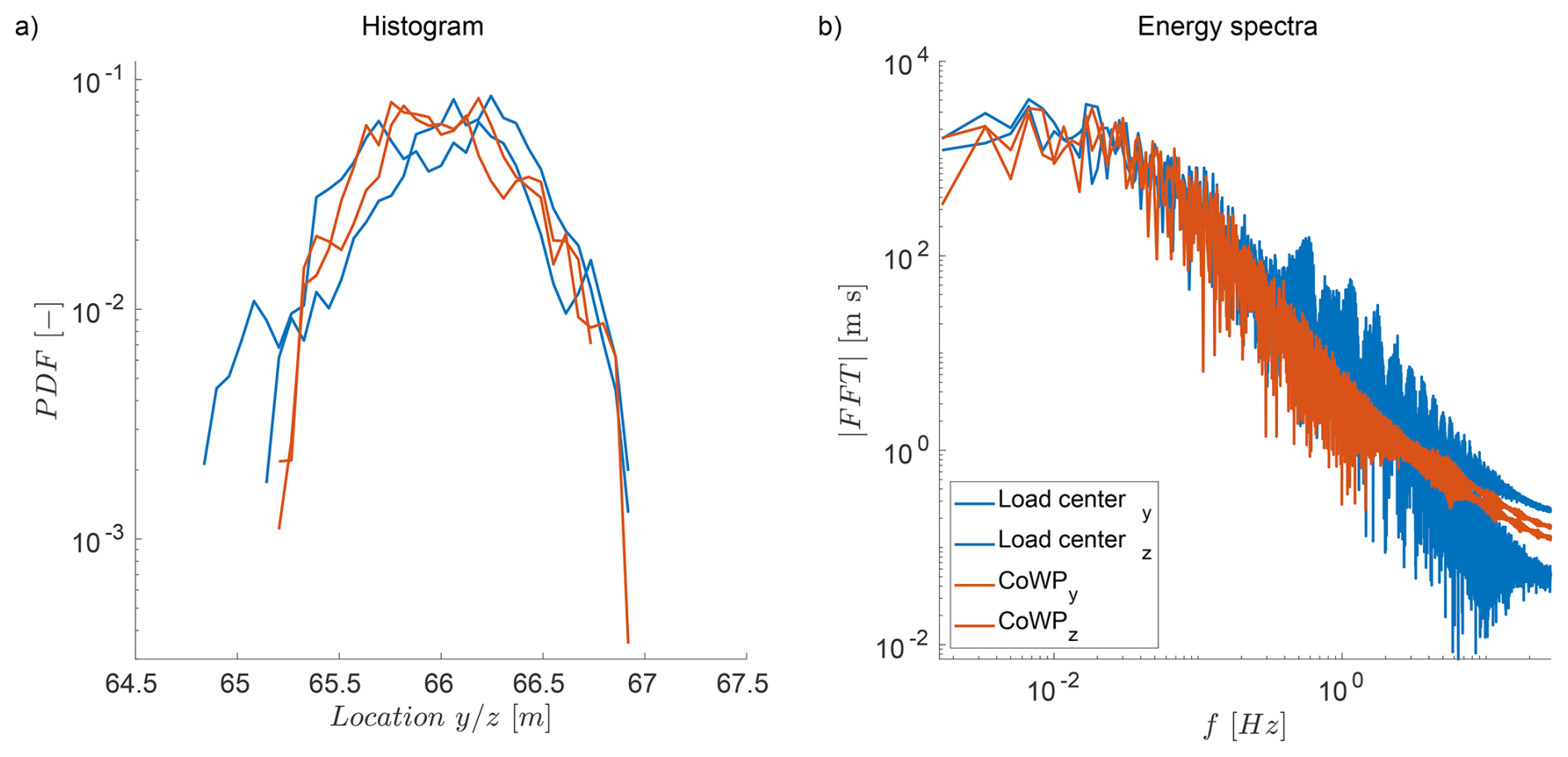
Figure 13 Statistical analysis histogram in (a) and energy spectra in (b) of the scaled CoWP and the filtered load centre for the BEM simulation (Fig. 12).

4.1 Uniform laminar flow

In the uniform laminar flow case, the inlet velocity is the same everywhere. Consequently, the position of the CoWP is in the centre of the rotor surface (derived Eq. 3). The course of the load centre in the BEM simulation is trivial, with zero in Y and Z, whereas the load centres for LES-AL and DDES-BL deviate slightly from the centre of the rotor, shown in Fig. 5. The standard deviation is $\mathrm{7.20}\times {\mathrm{10}}^{-\mathrm{3}}\mathrm{m}$ in Y and Z for LES-AL and $\mathrm{2.06}\times {\mathrm{10}}^{-\mathrm{2}}\mathrm{m}$ in Y and $\mathrm{1.99}\times {\mathrm{10}}^{-\mathrm{2}}\mathrm{m}$ in Z for DDES-BL. As can be seen in Sect. 4.2, 4.3.1, and 4.3.3, these fluctuations are 1 order of magnitude smaller than for the shear and turbulent case. Despite the minor deviation compared to the other flow cases, the causes are investigated in order to understand the intrinsic properties of the models.

In the LES-AL simulation, the fluctuations appear at the 3P frequency and can therefore be attributed to interpolation errors between the Cartesian grid and the rotational blades (see Fig. 6). On the other hand, the 3P frequency is defined as 3 times the rotational frequency of the turbine (=0.605 Hz). Those errors are a well-known characteristic of LES-AL simulations, which occur when the body forces are applied to the portion of the domain where the blades are; see Churchfield et al. (2017).

Finally, we examine the DDES-BL case. To explain the fluctuation in this case, we need the Q criterion (Davidson, 2015) and the sectional forces on the blade. Figure 7 visualises the isosurfaces of the Q criterion around the rotor for LES-AL in Fig. 7a and DDES-BL in Fig. 7b. In the LES-AL case, only the three helical tip vortices and a portion of the root vortices can be recognised. In the DDES-BL case, many small detached vortex structures appear near the blade root due to the turbine blade's cylindrical cross-section up to a radius of 8.3 m. The flow around this cross-section is typically detached, and each blade is strongly influenced by the wake of the others, so no periodic vortex patterns are formed.

Figure 8a and b show the time-averaged and time-dependent course of the sectional blade forces for the DDES-BL case. Figure 8c shows the relative standard deviation to the mean value over the blade length. In general, the sectional forces confirm the conclusions from the Q-criterion analysis. The forces near the blade root, where a cylindrical cross-section is present, fluctuate strongly, with a standard deviation of over 10 %. Further outwards, there is a transition segment to an airfoil (at half of the blade length), from which the forces are more or less constant with a relative standard deviation of less than 0.2 %.

The strong fluctuations in the forces at the blade roots cause the load centre to not always coincide with the centre of the rotor surface (Fig. 5). This offset, of the order of a few centimetres, results from the randomness of flow being detached/attached to the three rotor blades.

4.2 Laminar shear flow

Since there is a velocity gradient in the inlet for the shear case, the position of the CoWP is not straightforward. The calculated CoWP_Z is 3.39 m, and CoWP_Y=0 for the inlet boundary condition of the simulations.

Figure 9 shows the time series of the load centres for the different simulation methods. In contrast to the laminar case, the load centres fluctuate periodically for all methods. Due to the velocity gradient of the shear flow, the load on each blade varies during each revolution. Because the blades are geometrically coupled, the load centre rises when two blades are above the nacelle and falls when two blades are below it. The same applies to the Y component, corresponding to the blade position and the associated load centre. As can be seen in Fig. 10, the 3P frequency of revolution (0.605 Hz) is the dominant one for all simulation methods.

The mean load centre in the Z component is similar for BEM and LES-AL, with 1.13 and 1.16 m. The load centre for the DDES-BL simulation is substantially higher than the simulation models, with 1.66 m, where flow around the blades is not resolved. Now that we have the load centres from the actual forces and the CoWP from the boundary condition, we can determine the relationship between them. This relationship is used later in Sect. 4.3 as a calibration factor for the turbulent case. As already mentioned in the Introduction, this relationship was previously unclear. The mean values for the load centres and the ratio between the load centres and CoWP_Z are given in Table 3.

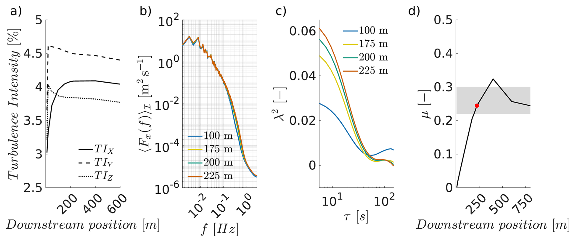
Figure 14 Analysis of turbulence without a turbine. Turbulence intensity over downstream position (a). Energy spectrum of different downstream positions (b). Shape parameters of the two-point statistics over the increment size (c). Downstream development of the intermittency parameter μ in (d).

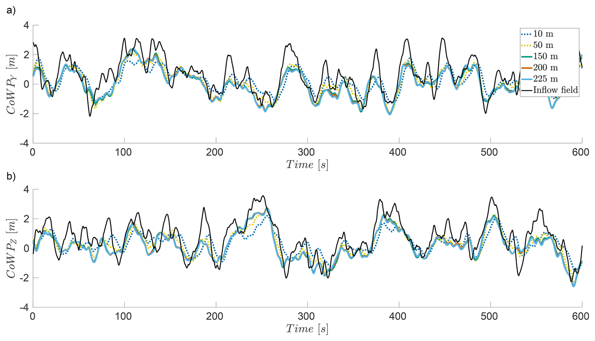
Figure 15 Time series of the CoWP in the inflow field (black) and at different downstream positions in an empty box LES (coloured). Y component in (a) and Z component in (b).

Similar to CoWP_Y, the mean load centre in the Y component is zero for BEM and DDES-BL (Fig. 9a). For LES-AL, the mean load centre is 0.12 m. The shift is related to the direction of rotation of the turbine, as shown in Appendix B.

4.3 Turbulent inflow

This section examines simulations involving turbulent inflow. In Sect. 4.3.1, the turbulent wind field is used as inflow for BEM. As already indicated in the Introduction, LES involves a spatial–temporal development of turbulence. Therefore, Sect. 4.3.2 first examines the turbulent field in a simulation without a turbine, and Sect. 4.3.3 then examines it with a turbine.

4.3.1 Turbulent case in BEM

The time series of the CoWP from the synthetic inflow field and the load centre from the BEM simulation are shown in Fig. 11. As with the laminar shear case from Sect. 4.2, the amplitude of the load centre is substantially lower than the CoWP. Furthermore, the load centre signal exhibits many fluctuations. Similar observations were described in the work of Moreno et al. (2025). In their work, the load component was filtered using a low-pass filter, and all signals were normalised to a standard deviation of 1.

Figure 16 Energy spectra of the LES flow field at different downstream positions.

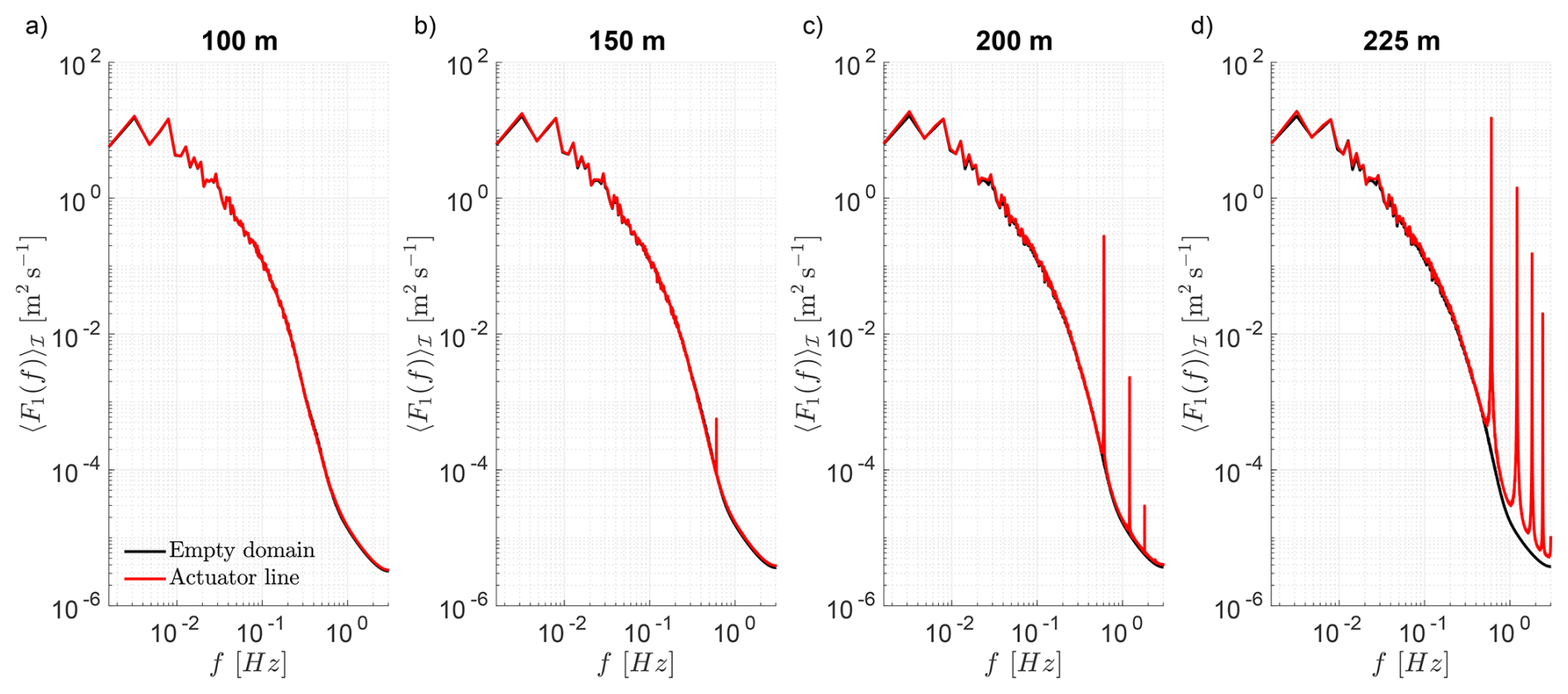
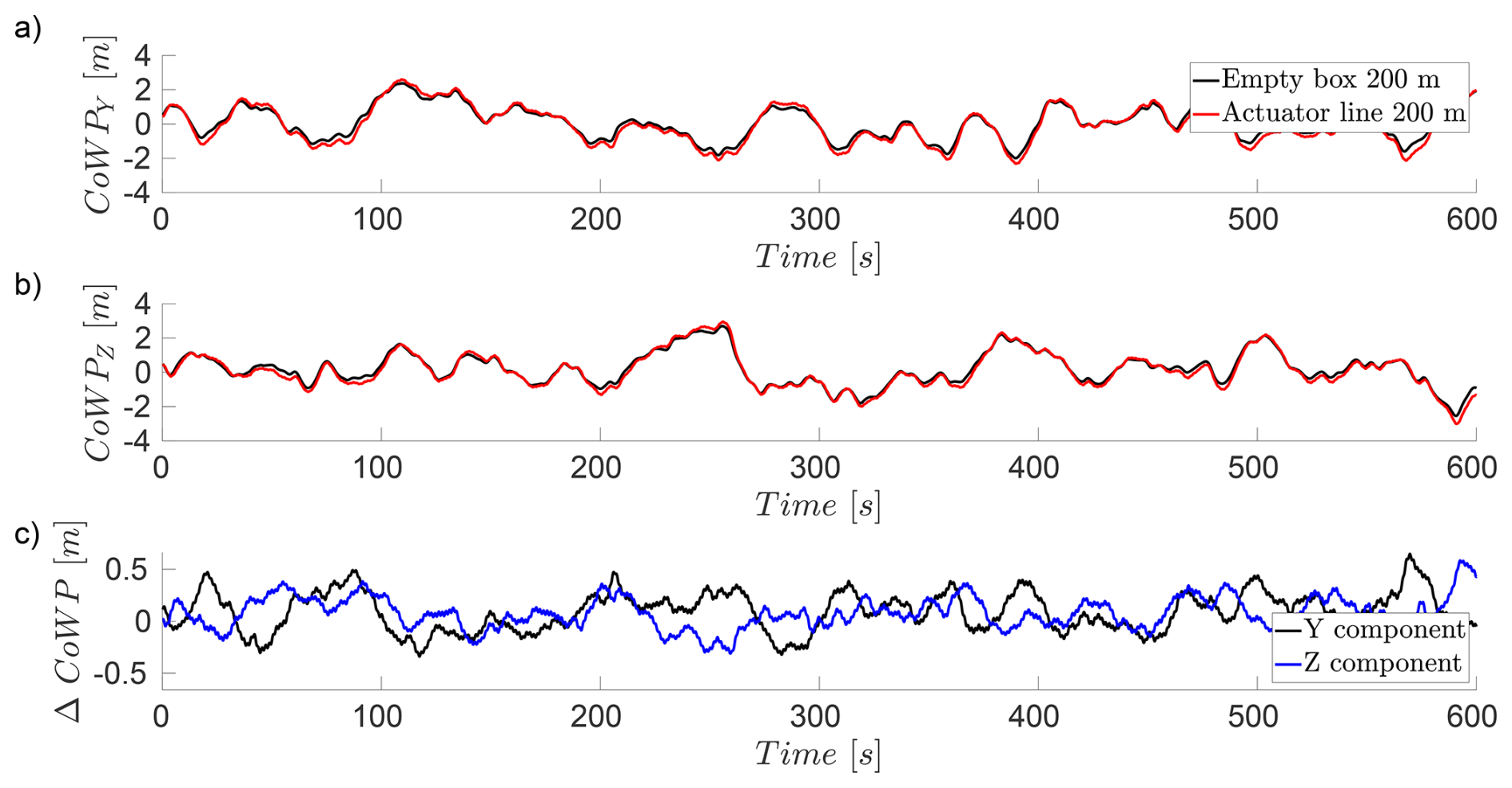
Figure 17 Time series of the CoWP 200 m downstream of the inflow without turbine (black) and with the LES-AL-modelled turbine (red) in (a, b). Absolute difference between the simulation with and without a turbine in (c).

In the present work, the load centre is also filtered using a low-pass filter with a cutoff frequency of 0.660 Hz (≈110 % of the 3P frequency). This frequency was selected in order to filter out the high-frequency components while still capturing the dominant 3P frequency (with an additional buffer of 10 %). In contrast to the previous work, a different method of normalisation is chosen here. The value of the CoWP is corrected through multiplication by the ratio ($\text{Load centre}/{\text{CoWP}}_Z$) under laminar conditions, given in Sect. 4.2 and Table 3. Figure 12 shows the time series of the filtered load centre and the rescaled CoWP. Filtering and scaling indicate a good correlation between the load centre and the CoWP, with a Pearson correlation coefficient of 0.814. Figure 13 shows the statistical analysis of the time series of the scaled load centre and the filtered CoWP. In both the histogram in (a) and the energy spectrum in (b), the load and flow variables have similar properties.

4.3.2 Turbulence characterisation in LES

Before discussing the results of the LES-AL-modelled turbine under turbulent inflow, a characterisation of the flow must be carried out first. Intermittency is an intrinsic property of turbulence. As shown by Bock et al. (2024), a realistic representation of a turbulent flow can only be achieved if these characteristics have been verified. Furthermore, the turbulence interacts with the induction zone and the blades of the turbine. In order to distinguish between and evaluate these two influences on the flow, a simulation without a turbine is carried out first, and the characterisation proposed by Bock et al. (2024) is performed. Afterwards, a comparison of the flow with a turbine is conducted.

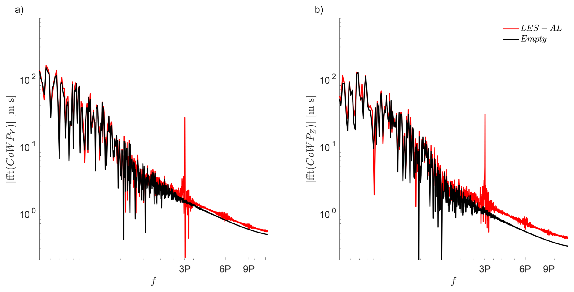
Figure 18 FFT of the CoWP in LES 200 m downstream of the inflow in an empty box (black) and with the AL-modelled turbine (red) (Fig. 17) (3P=0.605 Hz).

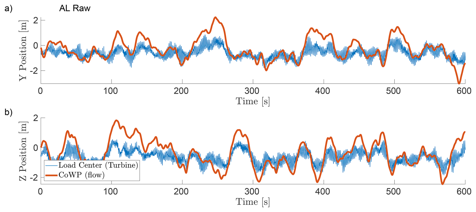
Figure 19 Direct comparison of the time series of the CoWP from LES in the rotor plane (orange) and the load centre of LES-AL (blue). Y component in (a) and Z component in (b).

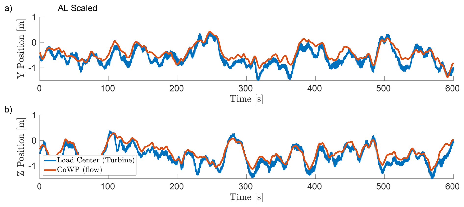
Figure 20 Direct comparison of the time series of the scaled CoWP from LES in the rotor plane (orange) and the filtered load centre of LES-AL (blue). Y component in (a) and Z component in (b). r_Pearson=0.908.

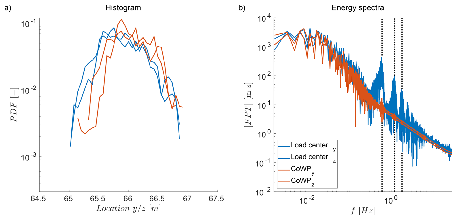
Figure 21 Statistical analysis (histogram in a) and energy spectra in (b) of the scaled CoWP and the filtered load centre for the LES-AL simulation (Fig. 20). The dotted vertical lines represent the 3P rotational frequency and its higher harmonics.

Figure 14 shows the characterisation of the turbulence at different downstream positions. The standard quantities, turbulence intensity (TI), and energy spectrum are shown in (a) and (b). Since there is no turbulence production, it is a case of decaying turbulence. As usual with a turbulent inflow, TI_x is lower than TI_y and TI_z after the inflow and increases within the first 100 m (Gilling and Sørensen, 2011; Bock et al., 2024; Keck et al., 2014). As expected, there are negligible changes in the energy spectra.

Now that two fundamental properties of a decaying turbulent flow have been confirmed, we examine the higher orders of the two-point statistics in Fig. 14c and d. In (c), the shape parameter λ² of the increment statistics over the increment size τ is presented, which quantifies intermittency. For small increments, the shape parameter is >0 and thus exhibits non-Gaussian or intermittent properties of the increment statistics. The intermittency parameter μ can be determined from λ(τ)² according to the K62 turbulence model (Kolmogorov, 1962; Obukhov, 1962; Chilla et al., 1996). A more detailed description of this method is given in Bock et al. (2024). The downstream development of the intermittency parameter is shown in Fig. 14d. The range of the intermittency parameter for ideal turbulence in accordance with Arneodo et al. (1996) is shown as a grey area. Furthermore, the distance between the inflow and the turbine from Sect. 4.3.3 is marked as a red dot. Overall, the behaviour of the turbulence in LES is consistent with the results from Bock et al. (2024), which means that a realistic intermittency state is present.

Figure 15 shows the time series of the calculated components CoWP_Y and CoWP_Z from the wind field at different downstream positions. The input field before injection is shown in black and in different colours for the different downstream positions in LES in (a) and (b). There is a reduction in the amplitude from the beginning in LES compared to the inflow. After that, there are further adjustments within the first 100 m (represented by the dotted lines) and essentially no changes between 150 and 225 m. Nevertheless, the LES reproduces the basic CoWP pattern.

Similar to the TI (see Fig. 14a), the CoWP in the LES changes after the inflow in the domain. This change mainly occurs within the first 150 m. Subsequently, the course of the CoWP changes only very little. In order to analyse this effect in more detail, a supplementary study was conducted, which is described in detail in Appendix C. As a first step, velocity jumps are used as inflow for an LES instead of synthetic turbulence. This indicates that the source term inflow converts accelerations better than decelerations (Fig. C2). A direct comparison of the velocity field of the inflow with the LES shows that this effect of poorer deceleration also occurs with synthetic turbulence (Fig. C3), which explains the deviations in the CoWP in Fig. 15.

4.3.3 Turbulent inflow with LES-AL

The same inflow field from Sect. 4.3.2 is used in the next step for a simulation with an LES-AL-modelled wind turbine. Before the loads are considered, the flow in front of the turbine is analysed and compared with the empty simulation.

Figure 16 shows the energy spectra for a domain with a turbine in red and for an empty domain in black in the LES at different positions. At 100 m, the energy spectra are essentially the same. At 150 m, the spectra at the low frequencies are also the same. At the higher frequencies, there is a peak at 0.605 Hz, which corresponds to the 3P rotation frequency and is due to the periodic fluctuation caused by the rotating blades. At 200 and 225 m, the energy at this frequency continues to increase, and higher harmonics of this frequency arise. However, no difference can be seen between the simulations with and without a turbine in the low-frequency amplitudes. This suggests that the large-scale structures that dominate the CoWP are only slightly influenced by the interaction with the turbine.

The time series for the CoWP in the LES is shown 200 m downstream of the inflow with and without a turbine in Fig. 17a and b. The absolute differences between the simulation with and without a turbine are shown in (c). The deviation between the simulation with and without the turbine varies by ±0.6 m with a mean in both directions below 0.1 m. Therefore, the interaction of the turbine with the incoming flow is quite relevant, since at some times the deviation is 0.5 m, while the absolute CoWP offsets from the rotor centre are only 1 to 2 m.

The FFT of the CoWP from Fig. 17 with and without a turbine is presented in Fig. 18. The figure indicates that the 3P frequency, which appears in the LES-AL case due to the resolved induction of the rotating blades, adds additional noise to the CoWP for a simulation with a turbine. As can be seen from the energy spectra and the CoWP, the blockage caused by the rotating blades has an influence and possibly interacts with the turbulence. This raises the question of whether the rotor position influences the loads.

Figure 19 shows the time series of the CoWP from LES in the rotor plane and the load centre for the LES-AL simulation. As with the BEM simulation (Fig. 11), the load signal is noisy, and the maxima of the CoWP exceed the peaks of the load centre. As in Sect. 4.3.1, the load signal is filtered and the CoWP signal is rescaled with the calibration parameter from Sect. 4.2 (Table 3, Fig. 20). The correlation between the CoWP and load centre in LES-AL is even better than that in the BEM simulation, with a Pearson correlation coefficient of 0.908. This difference arises because the flow field for the CoWP calculation from the LES is actually the one that hits the turbine, whereas in the correlation from Sect. 4.3.1, the inflow wind field is modified slightly by the BEM simulation's induction model. The histograms and energy spectra also fit; see Fig. 21. As already shown in the investigation of the influence of the turbine, there are influences of the rotation in the form of peaks at the 3P frequency in both the load centre and the CoWP spectrum (3P and multiples shown by dashed lines).

5 Conclusions and outlook

In this work, three wind turbine models with different fidelities were compared in terms of their correlation to the load prediction from the CoWP. The CoWP itself is a new quantity purely extracted from the inflow wind field and therefore does not contain any information about the turbine or the local blade aerodynamics. Thus, two main questions had to be answered: first, how can the CoWP be converted into a load signal to be used in the development process of a turbine, and, second, is the concept described in the first two papers on CoWP also valid for high-resolution LESs?

The load centre is introduced, for BEM and LES-AL, to estimate the position at which the total aggregated thrust force acts on the rotor plane. The calculation of the load centre is derived from the CoWP concept by replacing the wind velocity with the sectional thrust forces. For the DDES-BL, this load position is given by the CoP. The load centre can be used to establish a connection between the flow-dependent CoWP and the turbine loads.

A turbine-specific calibration parameter can be determined from a laminar shear flow simulation. This single parameter summarises the relationship between the flow and the turbine loads. This methodology facilitates the prediction of load signals through the calculation of the CoWP in a turbulent wind field and subsequent scaling with the calibration parameter.

It has been shown that the methodology of using a calibration parameter derived from a laminar shear flow can also be applied to high-resolution LESs to scale the CoWP and obtain a load signal. In the LES-AL case, correlating the CoWP from the flow field just upstream of the turbine with the loads improves the agreement between the flow and the loads. This improvement arises because the interaction of the wind field with the induction zone is taken into account.

Nevertheless, further questions emerge directly from this work. What influence does the fluid–structure coupling of the blades have on the load centre and the CoWP? Does the CoWP analysis method work when two turbines are arranged in sequence or when several turbines form a wind farm?

Appendix A: Grid study

Several LES-AL simulations are carried out to determine the required grid resolution. The division of the refinement regions and the relative gradation to each other are kept the same. This makes it possible to vary the overall resolution through a single parameter in a comprehensible manner. The power coefficient of the turbine (C_P) over the overall number of cells is shown in Fig. A1. From the 3.5 million cell mesh, C_P seems to be saturated. The same basic mesh is also used for the DDES-BL simulations with a higher complexity. To be able to represent this complexity, the next finer mesh with 27.2 million cells was selected for this work.

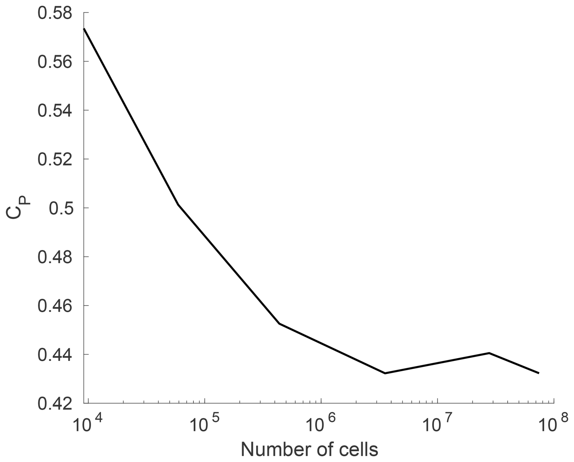
Figure A1 Power coefficient C_P for different grid resolutions in LES with the LES-AL-modelled turbine.

Appendix B: Impact of the rotational direction in LES-AL

Figure B1 shows the time series of the load centre in a clockwise simulation (red) and an anticlockwise simulation (blue). At the start of the simulation, the velocity field still corresponds to the initial values everywhere. As the flow field around the rotor and the wake develops, the two simulations approach the final values within the first 40 s. This corresponds to an estimated wake size of roughly 2D, which corresponds to the near-wake size (assuming the wake propagation speed is 55 % of the freestream velocity at hub height). The Z component of the load centres then become saturated for both directions of rotation to the value specified in Sect. 4.2 (since the courses are identical, only one line is visible.). In the Y direction, saturation occurs in opposite directions but with the same distance from the rotor centre. As with the fluctuations in the laminar case (Sect. 4.1), this shift in the load centre could be due to the smearing errors described in Churchfield et al. (2017). Since the focus of this work is on the analysis of the CoWP, this result is illustrated here as a property of the LES-AL method without further elaboration on the causes.

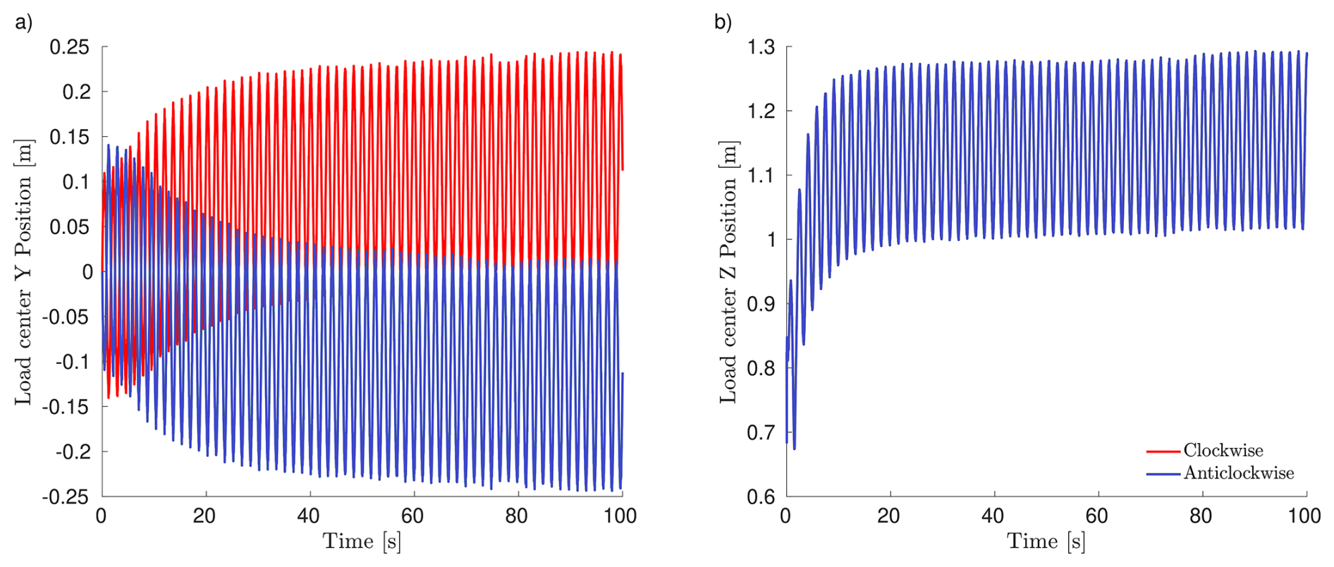
Figure B1 Time series of the load centre for LES-AL simulations with different rotational directions.

Appendix C: Turbulent inflow method

In order to determine where the differences in the CoWP between the inflow and the LES (Fig. 15) are coming from, an analysis of the turbulent inflow method is done here. Therefore, an LES with a velocity jump is done. Figure C1 shows the time-averaged velocity field in the sectional view of such a simulation. A total of 10 different velocity jumps in a range from −2 to 2 m s⁻¹ are carried out. This range covers 99.6 % of the fluctuations from the inflow field of the turbulent case from Sect. 4.3.3 ($U_{\text{mean}}=\mathrm{11.4}\mathrm{m}{\mathrm{s}}^{-\mathrm{1}}$, TI=5 %, Gaussian distribution of fluctuations).

Figure C2a shows the averaged velocity for the different velocity jumps. For a positive velocity jump, i.e. an acceleration (full line), a power law behaviour is observed as the flow reaches the target velocity. This is reached from 80 m after the inflow and remains constant until the outlet. With a negative velocity jump, i.e. a deceleration (dashed line), the behaviour is different. In contrast to intuition, the velocity increases within the first 50 m and then drops sharply but also reaches the target value after 80 m, as in the acceleration case.

Figure C2b shows a scatter plot of the targeted velocity jump over the achieved velocity jump. Accelerations are marked with circles and decelerations with triangles. It can be seen that the absolute deviation for small jumps ($<\mathrm{1}\mathrm{m}{\mathrm{s}}^{-\mathrm{1}}$) is smaller than for larger ones and that the achieved velocity jump diverges further from the target value for larger decelerations. The relationship between the achieved and targeted velocity jump can be represented by a quadratic fit, as shown with the black line.

Using the results from the simple simulations with velocity jumps, the CoWP curves of the input fields and the LES are compared again qualitatively. Figure C3a and b show the CoWP curve for the input field in black and for the LES 225 m after the inflow in green. Two points in time t₁=101 s and t₂=280 s are identified for further analysis. At both times, CoWP_Y is away from the centre. At t₁, the total deviation between the LES and the input field is only 1.01 m, and at t₂ it is 1.76 m.

Figure C3c and d show velocity sections for these two time points and the location of the CoWP for the inflow field. Figure C3e and f show the same for the LES. It is important to note that the TI decreased during transport through the domain (see Fig. 14). This can easily be observed when comparing (c) with (e), where the range of velocities $>\mathrm{12.5}\mathrm{m}{\mathrm{s}}^{-\mathrm{1}}$ in the LES is considerably smaller than in the input field. Furthermore, the range of velocities $<\mathrm{11.4}\mathrm{m}{\mathrm{s}}^{-\mathrm{1}}$ at the right or upper-right boundary is noticeably larger in the LES than in the input field. This can be explained by the fact that the Taylor hypothesis is only partially applicable Jacobitz and Schneider (2024). Due to transversal velocity components, transversal shifts occur.

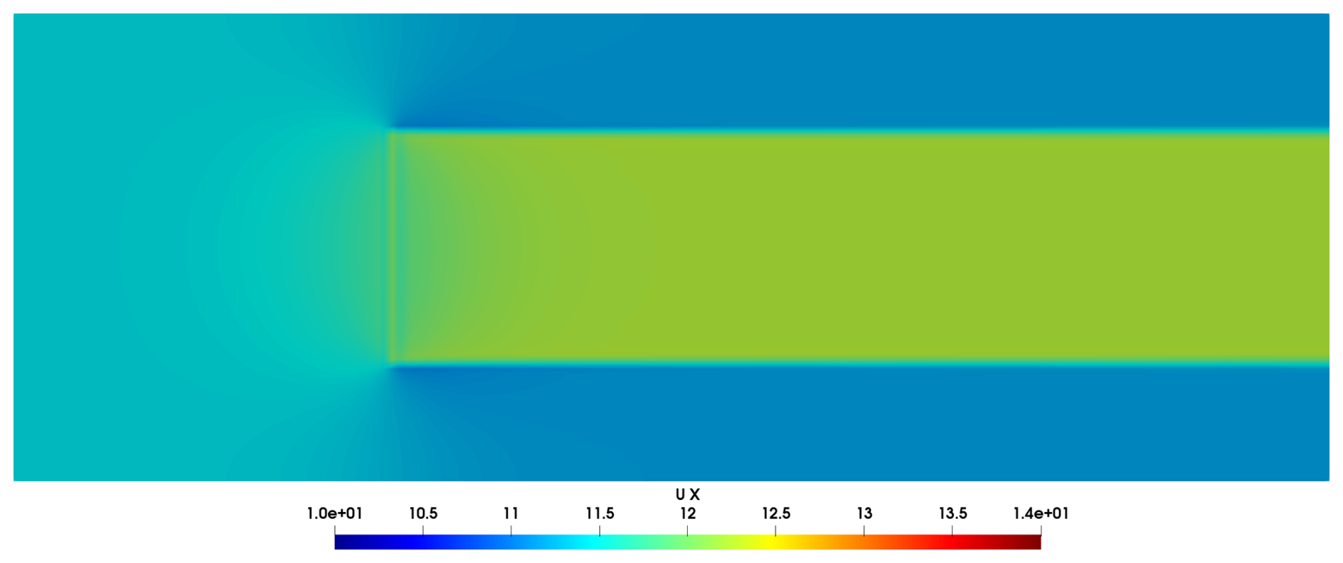
Figure C1 Time-averaged velocity field from an LES with a velocity jump achieved by an actuator.

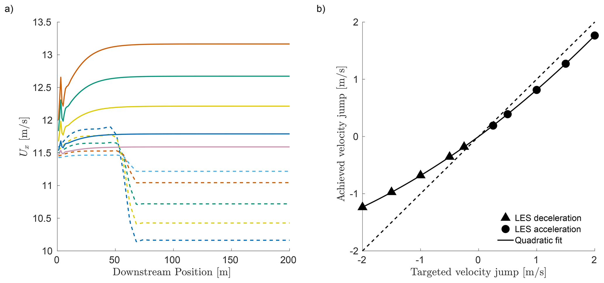
Figure C2 Time-averaged velocity over downstream position. (a) Scatter plot of the targeted velocity jump over achieved velocity jump (b).

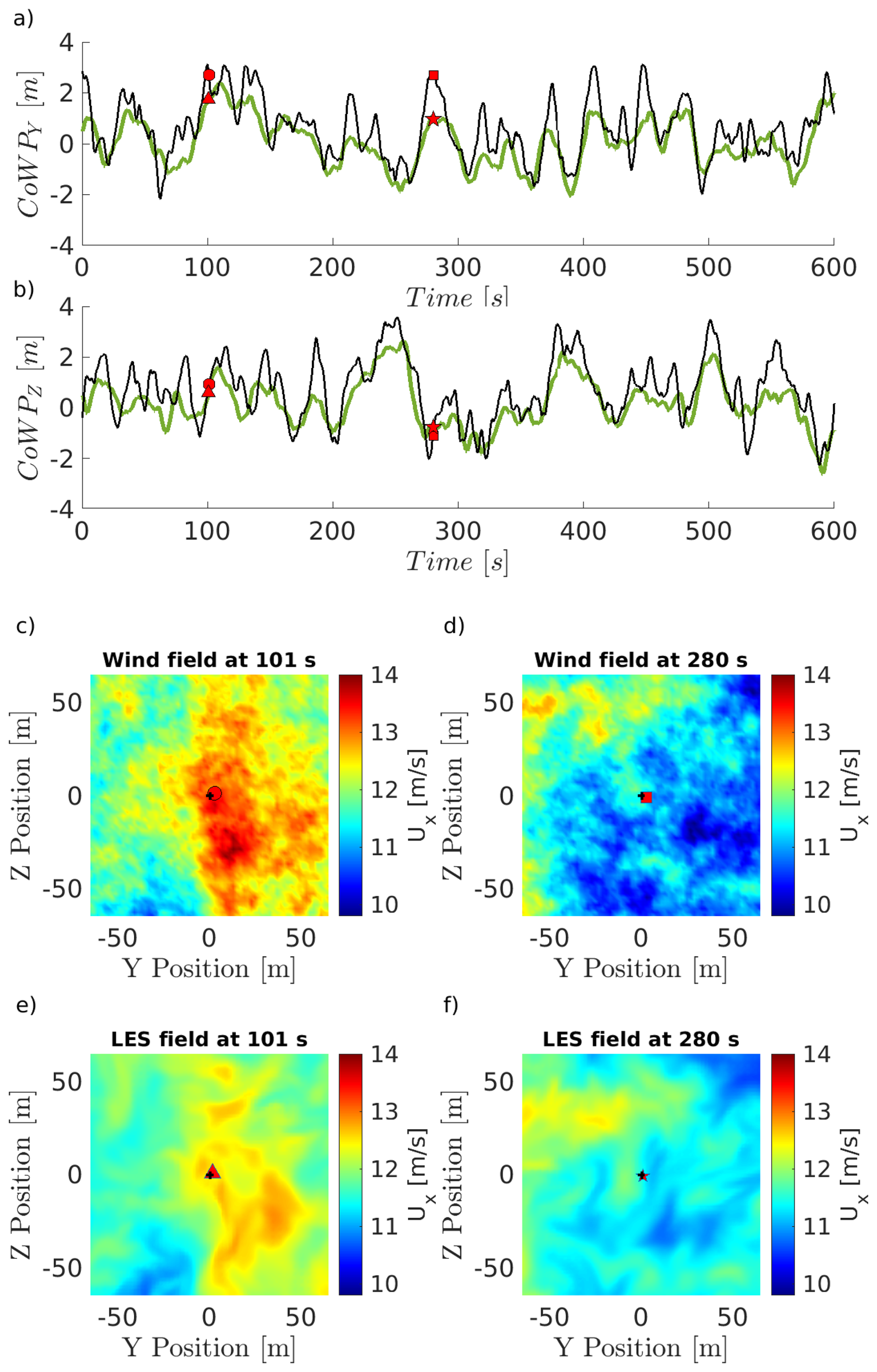
Figure C3 Time series of the CoWP of the input wind field (black) and in LES after 225 m. Velocity plane of the wind field at t₁ 101 s for the input field in (c) and in LES in (e). Velocity plane of the wind field at t₂ 280 s for the input field in (d) and in LES in (f).

Appendix D: Parameter study for the turbulent inflow

Table D1 Correlation factor between load centre and CoWP for different turbulent fields in BEM simulations.

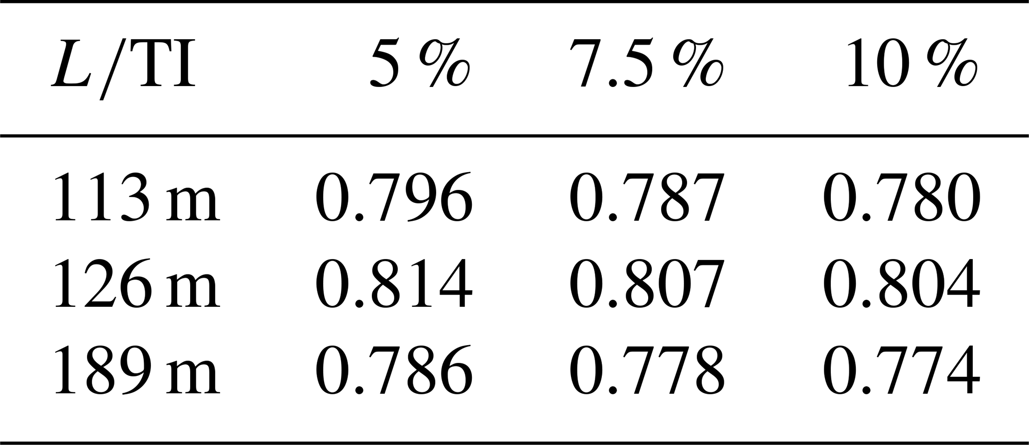
Table D2 Correlation factor between load centre and CoWP for different turbulent fields in LES-AL simulations.

For a generalisation of the results of this work, simulations with different turbulence parameters are carried out here. Three different integral lengths (113, 126, 189 m) and three TIs (5 %, 7.5 %, 10 %) are combined in BEM simulations. The procedure introduced in Sect. 4.3.1 is used for each combination. The time series of the load centre is filtered with a low pass, and the CoWP is scaled with the factor from Table 3. Table D1 shows the values for the Pearson correlation coefficients.

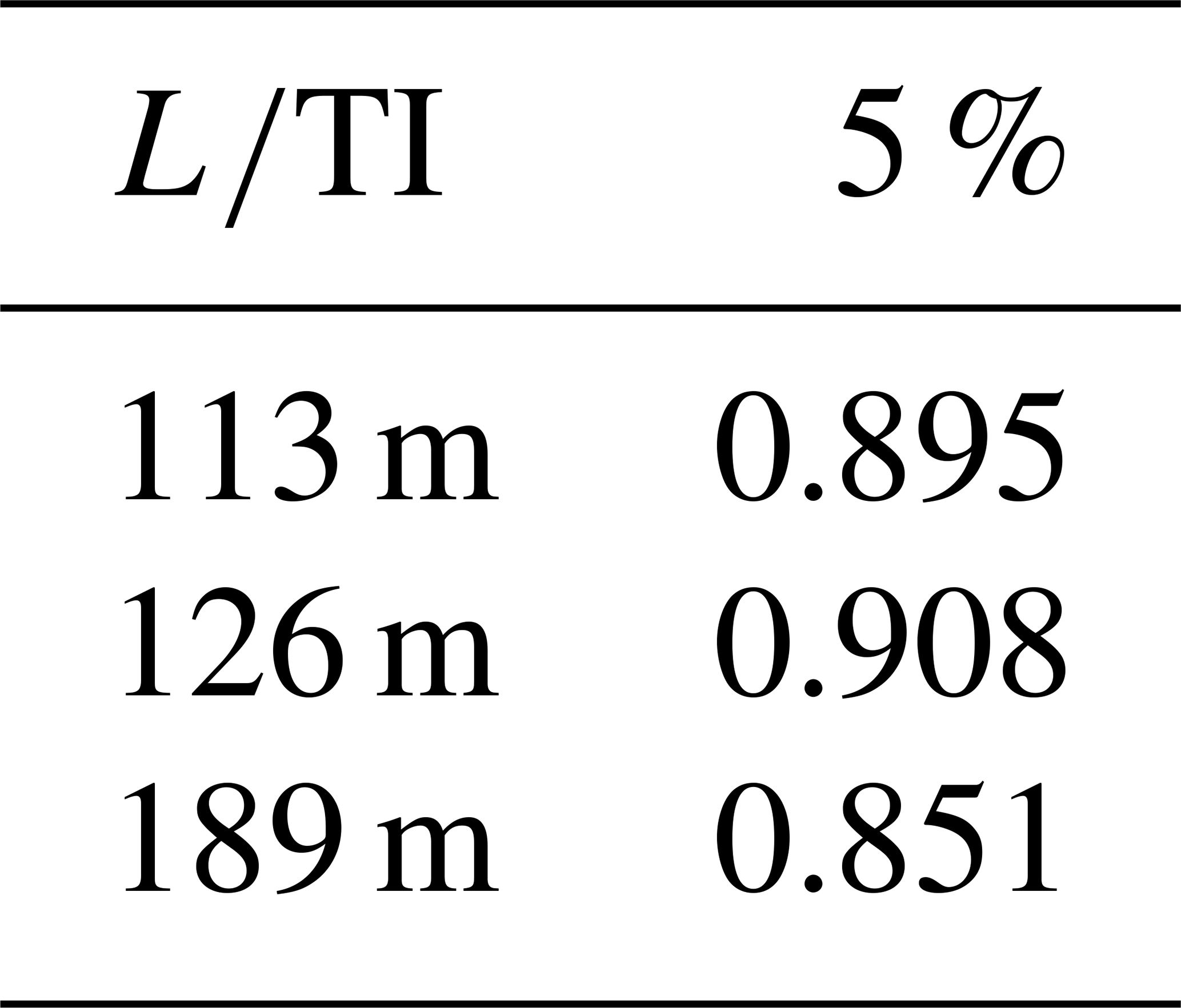
Due to the greater computational effort of LES-AL simulations, only one TI with three integral lengths are simulated. The Pearson correlation coefficients are presented in Table D2.