Uncertainty in North Sea offshore wind power: contributions of reanalysis forcing, turbine type, and wake parameterization

With the transition towards green energies gaining momentum, the expansion of wind farm areas and associated technologies is growing fast. The North Seas Energy Cooperation group has set an ambitious target to increase the offshore wind-generated power capacity from 26 GW in 2022 to 300 GW by 2050 in the geographical areas of the North Seas. With this goal, an extensive offshore infrastructure is planned to be deployed in the region. Studies have been carried out to assess the power production of such future development. However, the associated uncertainties are often only partially addressed due to the complexity and diversity of contributing factors, ranging from technical aspects such as turbine geometry and layout to atmospheric processes across multiple scales, from small-scale turbulence to mesoscale dynamics. Wake effects have been identified as the primary source of power losses. They are often studied in individual wind farms or small clusters, but the dynamics of large wind farm clusters at a regional scale are only beginning to be explored. In this study, we address uncertainties of power output derived from projected wind farm areas in the North Sea in scenarios that encompass different turbine setups and boundary conditions. To achieve this, we used COSMO6.0-CLM, the newest version of the regional climate model COSMO-CLM, and further improved the existing wind farm module to extend the model's capability to design more flexible and realistic scenarios. This allows us to quantify impacts from different factors that contribute to power output uncertainties. Our analysis indicates that the combined uncertainty due to driving conditions and the difference of turbine types amounts to approx. 15 GW, corresponding to 10 % of the total installed capacity (150 GW). Of this, the contribution from driving conditions accounts for 2.5 %, whereas the difference of turbine types has a larger influence, contributing roughly 7.5 %. After applying a correction factor (0.25) to the turbulence production term from the Fitch wind farm parameterization, we found that this modification translates to a reduction in power output of roughly 2 GW (about 1 % of the installed capacity). Given that economic evaluations, environmental assessments, and energy policy decisions make use of modelled wind power outputs in their analyses, accounting for these uncertainties would help to ensure more reliable results.

1 Introduction

The ambitious goal of the European Union to be climate neutral by 2050 has triggered an increasing demand for the production of renewable energy. Many European countries have expanded their plans to use wind energy as part of the solution (NSEC, 2021; Bundesregierung, 2022). According to the renewed political declaration from the North Seas Energy Cooperation group (NSEC), the total offshore installed capacity in Europe is planned to further increase from approx. 26 GW in 2022 to at least 60 GW by 2030 and 300 GW by 2050 (NSEC, 2021). As part of the strategy to achieve this goal, the development of large wind farm clusters across the North Sea region is being fostered. However, such a large-scale deployment will induce mutual influence between wind farms, which may negatively impact their performance, leading to a greater reduction in electricity production than initially anticipated. Uncoordinated development could also lead to significant losses of expected electricity generation. Developments in multiple countries could influence each other, requiring international treaties on transboundary resources, similar to freshwater, oil, and fisheries (Lundquist et al., 2018). Moreover, previous studies have shown that the effects of the wakes produced from wind farm areas can cause local and regional changes in the marine environment, for example, impacts on the atmospheric circulation (Hasager et al., 2015; Akhtar et al., 2021), the ocean circulation (Ludewig, 2013; Christiansen et al., 2023), and the ecosystems (Daewel et al., 2022; Gușatu et al., 2021). Therefore, a comprehensive understanding of wake interactions at regional scales, particularly in large wind farm clusters, is essential for assessing their impacts and associated uncertainties.

Numerous observational and numerical studies have examined the implications of wake effects, particularly in the energy sector, where power output losses play a significant role in economic planning. This remains a state-of-the-art topic, as highlighted by several contributions at the 5th Wind Energy Science Conference (WESC, 2025). Wake effects can substantially reduce wind farm efficiency (also called capacity factor) and decrease overall energy production (Lee and Fields, 2021; Kelly, 2025). Since the sector is still under development, many of these studies are often focused on a single turbine or single wind farm rather than a regional-scale system. Reports indicate values of capacity factor from single onshore wind farms of 26 % in the UK (Waters, 2023), 55 % in Poland (Olczak and Surma, 2023), and 21 % to 55 % (with an approximated mean value of 35 %) in the US (Wiser et al., 2022). Meanwhile, for offshore wind farms in Europe and the US, the capacity factor is estimated to be 23 % to 52 % (with an average of 35 %) (Cai and Bréon, 2021; WEO, 2019; Menezes, 2019; Stehly et al., 2018; Waters, 2023; Cassa, 2024; Smith, 2024). However, studies that address power losses in clusters are rather limited; Nygaard (2014) and Nygaard and Hansen (2016) found that, using observational data from a wind farm in Denmark, its efficiency was reduced by up 10 % to 16 % in the direction range from where a neighbouring wind farm was newly constructed. Lundquist et al. (2018) estimated a power loss of downwind wind farms by 5 % from observation data for a specific month (January 2013). A more comprehensive approach is presented in Akhtar et al. (2021), where a 10 year transient climate simulation incorporates single-size turbines (5 MW) distributed across operational and planned wind farm sites in the North Sea using a numerical model with the Fitch wind farm parameterization (Fitch et al., 2012). They estimate a mean reduction of the capacity factor of 20 % for the North Sea wind farms. In more recent studies, Akhtar et al. (2024) and Borgers et al. (2024) compare the increment on the capacity factors by upgrading the rated power of the simulated turbines from 5 to 15 MW. Akhtar et al. (2024) report an increment of 2 % to 3 %, whereas Borgers et al. (2024) estimates the increment to be about 9 %. The variability can be attributed to the distinct nature of each study; however, a fair comparison of the results is challenging due to differences in locations, wind farm configurations, wake calculation methods, atmospheric conditions, turbine specifications, and other factors, but at the same time, this highlights the significance of the uncertainty in such assessments.

To investigate and quantify the variability and uncertainty of wake effects, we conducted simulations following a similar approach to Akhtar et al. (2021). The numerical model was further refined to account for different turbine specifications and to integrate wind farm metadata (Elizalde, 2023). These enhancements enable the representation of more realistic wind farm configurations, incorporating a non-homogeneous distribution of turbine characteristics and time-based activation of wind farms under otherwise identical conditions. To validate the model, a spatial and temporal variability analysis of wind speed was performed.

With respect to boundary conditions, Hahmann et al. (2022) compared wind speed estimates from four reanalysis products (NEWA, ERA5, MERRA2, and 20CRv3) with mast observations from several offshore platforms in the North Sea (FINO1, FINO2, FINO3, IJmuiden, and Ekofisk) over the period from 1980 to 2014. Their analysis showed that, when evaluated in relation to the observational data (see their Fig. 2), the wind climates produced by the different reanalyses were “nearly identical”, with mean values ranging from 10.0 to 10.2 m s⁻¹. To investigate for these small uncertainties associated with the choice of boundary conditions and their impact on power production, our scenarios were driven using two different reanalysis datasets (ERA-Interim and ERA5). All simulations assumed a total installed capacity of 150 GW for the North Sea region, consistent with the mid-range targets outlined in the NSEC plans.

Building from these results, the present study examines how minor discrepancies introduced by different driving datasets affect power production.

The structure of the paper is as follows: Sect. 2 describes the data sources used for turbine specifications, wind farm metadata, and observed wind speeds for model validation. Section 3 presents enhancements to the wind farm scheme within the COSMO-CLM climate model (Rockel et al., 2008) and details the simulated scenarios. Model validation, as well as the analysis of wake effects and power losses, are discussed in Sect. 4. Finally, conclusions are provided in Sect. 5.

2 Data

2.1 Turbines specifications

As part of the new approach in our wind farm simulations, within the atmospheric model COSMO6.0-clm, we enable the distribution of different turbine specifications (power capacity, hub height, and rotor diameter) over the simulated domain. Turbine information was obtained from the National Renewable Energy Laboratory Turbine Archive (NREL, 2020) and Wind Turbine Model database (WTM, 2020), and are listed in Table 1. The databases provide turbine dimensions, tabular curve data for wind-speed-dependent idealized power output and thrust, and power and thrust coefficients for onshore and offshore turbines. The coefficients correspond to those used in the wind farm parameterization to calculate momentum sink, turbulent kinetic energy, and power output (Sect. 4). However, NREL (2020) reports that power curves calculated from power coefficients deviate from idealized power output due to “a number of reasons”, without further details. This discrepancy was corrected by scaling the provided power coefficients to fit the expected values. The scale factor (the ratio between the idealized power and uncorrected power above-rated wind speeds) for each turbine is shown in Table 1, and the respective power curve is depicted in Fig. 1. The unevenness of the calculated power curves at above-rated wind speeds is the result of larger gaps in the provided uncorrected tabulated coefficients. Modern turbines have power curves that reflect control strategies around the cut-off wind speed, allowing them to operate beyond such a threshold. These control strategies are not considered in the NREL or WTM data, nor included in the parameterization developed here. In our case, the turbine shutting is simulated by setting to zero the power coefficient above the cut-off speeds and by using the last value before the cut-off for the thrust coefficient.

Table 1 Turbine specifications from NREL and WTM used for the atmospheric simulations with different technical scenarios. The scale factor denotes the correction applied to each turbine tabulated data from NREL and WTM databases to better align with their idealized rated capacity.

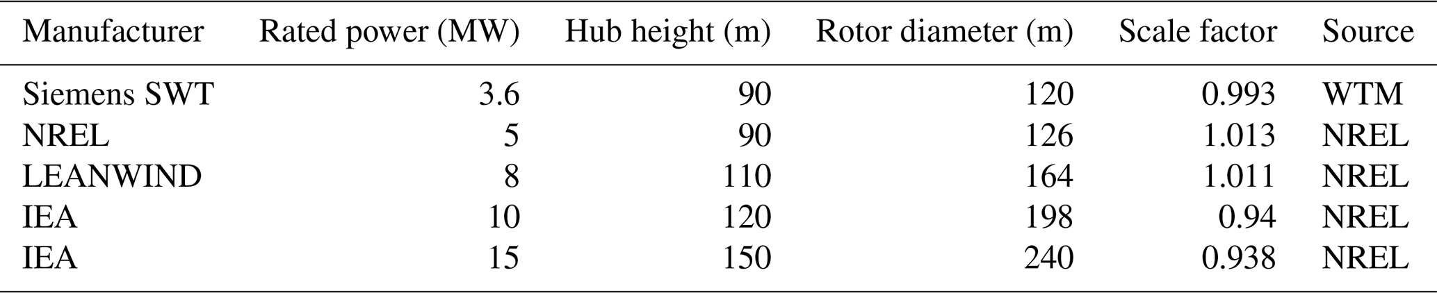
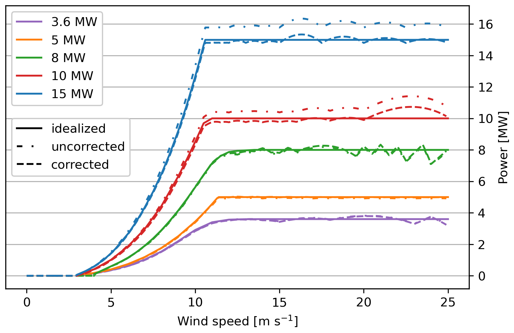
Figure 1 Power curves for turbines with different rated capacities. Idealized power (solid lines), uncorrected curves calculated directly from the provided turbine power coefficients (dashed-dotted lines), and corrected curves obtained following the application of the scale factor (dashed lines).

2.2 Wind farm metadata

The wind farm metadata were updated from the previous model version. The European Marine Observation and Data Network information (EMODnet, 2022), supported by the European Union's Integrated Maritime Policy, has been incorporated into the COSMO6.0-clm model. This open-source dataset is continuously maintained on a monthly basis with new information as it becomes available. The data used in this study correspond to the version available at the time of access in March 2022. The dataset provides information on the status of each wind farm area (in production, in construction, approved, planned, etc.) and the geographical location of its boundaries. Detailed specifications are not available for all wind farms, especially not for those in planning status. In such cases, the turbine specifications for the highest rated capacity (15 MW) were used. Figure 2 shows the model domain and the distribution of the wind farm areas with their corresponding rated power based on EMODnet data. Those areas are relative to the planned areas, which do not necessarily correspond to the actual construction areas. Details on turbine distribution, density, and the precise location of the construction area were not available, at least not at the time of EMODnet data acquisition. Wake and its effects may vary depending on turbine distribution and location. In this work, we assume that turbines are evenly distributed across their respective planned areas.

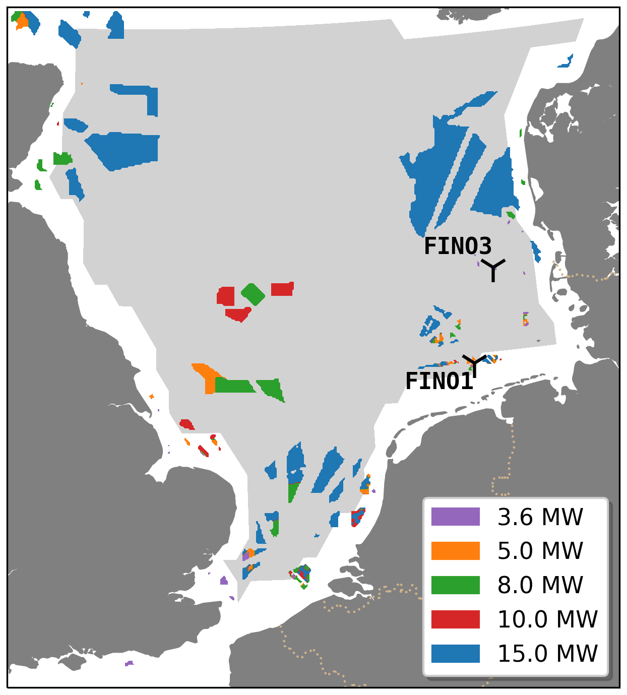
Figure 2 Spatial distribution of planned wind farm areas and their rated capacities, according to EMODnet dataset (accessed in March 2022). The black markers show the location of observational platforms FINO1 and FINO3. The shaded grey region in the North Sea denotes the area employed for the statistical validation of the 10 m wind field described in Sect. 4.1.

2.3 Wind speed observations

The Advanced Scatterometer (ASCAT) satellite-based data (Ricciardulli and Wentz, 2016) are used to evaluate the spatial variability of the simulated wind. It is a modified version of the daily EUMETSAT MetOp-ASCAT ocean surface wind vector product v02.1, released by Remote Sensing Systems in April 2016 (Ricciardulli and Wentz, 2016). Remote sensing techniques are used to compute near-surface wind vectors at 10 m height above the ocean surface by measuring the sea-surface backscattering signal due to the roughness of the sea surface (Gelsthorpe et al., 2000). It provides two daily measurements: one from the ascending pass and one from the descending pass. The dataset has a spatial resolution of 25 km and a temporal coverage period from 2007 to the present. For the model validation period from 2013 to 2018, we utilized data from the MetOp-A mission only.

For the validation of the temporal variability, hourly wind speed data are obtained from the FINO1 and FINO3 research platforms (Westerhellweg et al., 2012; Leiding et al., 2016) in the North Sea, provided by the Bundesamt für Seeschifffahrt und Hydrographie (BSH) (BSH, 2023). The dataset consists of mast corrected 10 min mean values derived from sonic and cup anemometers installed at eight to nine measurement heights ranging from 21 to 107 m. FINO1 is located at approx. 45 km north of Borkum at coordinates $\mathrm{54}\mathit{°}{\mathrm{00}}^{\prime }{\mathrm{53.5}}^{\prime \prime }$ N, $\mathrm{6}\mathit{°}{\mathrm{35}}^{\prime }{\mathrm{15}}^{\prime \prime }$ E in the immediate vicinity of an operating wind farm cluster composed by Alpha Ventus, Borkum Riffgrund I and II, the westbound TranelWindpark Borkum and Mercury with other wind farms in the vicinity under construction. FINO3 is located 80 km west of Sylt with a potential influence of onshore wind turbines at the coast and nearby operating offshore wind farms of Butendiek, DanTysk, and Sandbank.

Simulated wake effects were compared with airborne measurements from the German Research project WInd PArk Far Field (WIPAFF) (Emeis et al., 2016; Platis et al., 2020). The field campaign consisted of 41 flights in different wind farm locations at specific times and altitudes. The research aircraft recorded all components of wind speed, humidity, temperature, and pressure at a sampling frequency of 100 Hz. In this work, flight number 7, dated 10 September 2016 from 08:00 to 11:00 UTC, was selected as it captured the main characteristics of the wake extension at hub level (90 m) between the cluster formed by the wind farms of Amrumbank West, Nordsee Ost, Windpark Meerwind SuedOst, and Butendiek, located 50 km to the north of the cluster (Baerfuss et al., 2019). This makes it a good case study for comparing model results (see Sect. 4.3).

3 Methods

3.1 Atmospheric model

The atmospheric model COSMO-CLM (Rockel et al., 2008) is a non-hydrostatic limited-area model widely used in climate research (e.g. Sørland et al., 2021). It describes a compressible flow in a moist atmosphere based on thermo-hydrodynamical equations. The equations are solved numerically with a Runge–Kutta time-step scheme (Wicker and Skamarock, 2002) at meso-β and meso-γ scales (2 to 200 km) (Steppeler et al., 2003). This is done on a three-dimensional grid according to the Arakawa-C scheme with a Lorenz vertical grid staggering (Arakawa and Lamb, 1977). The grid is defined on rotated geographical coordinates with a terrain-following height coordinate (Doms et al., 2013). Initial and lateral boundary conditions are imposed by a driving host model. At the upper levels, a sponge layer with Rayleigh damping is used, whereas lateral boundary conditions use a one-way nesting by Davis-type formulation. The sea surface temperature is prescribed by the forcing data. Horizontal and vertical advection are treated explicitly; tendencies are evaluated by taking advection velocities, kinetic energy, and absolute vorticity at the centred time level n of the leapfrog scheme. The scheme for vertical turbulent transport at the sub-grid scale is based on a second-order closure at hierarchy level 2.0 (Mellor and Yamada, 1974). The standard physical parameterizations include the radiative transfer scheme (Ritter and Geleyn, 1992), Tiedtke parameterization for convection (Tiedtke, 1989), and a turbulent kinetic-energy-based surface transfer and planetary boundary layer parameterization (Raschendorfer, 2001). The land–atmosphere interaction is represented by the TERRA multi-layer soil–vegetation–atmosphere transfer scheme, which explicitly resolves heat and moisture transport in soil, snow, and canopy layers. TERRA ensures the closure of the surface energy and water balance by simulating soil temperature and moisture dynamics, evapotranspiration, and snowpack evolution, and the surface fluxes of heat, moisture, and momentum (Schrodin and Heise, 2001; Schulz et al., 2016; Schulz and Vogel, 2020).

The wind farm parameterization developed in COSMO5.0-clm15 (Akhtar and Chatterjee, 2020) has been implemented in the COSMO6.0-clm version (Elizalde, 2023) (see Sect. 3.2). COSMO6.0-clm is the final COSMO version and the result of the unification of all developments in physical parameterizations of the numerical weather prediction and the climate mode. The model structure of the physical parameterization was changed to the structure of the most recent numerical model ICON (Doms et al., 2021). The updated schemes consist of the prognostic variables for the microphysics (water vapour, cloud water, ice, rain, snow, and graupel) (Doms and Förstner, 2004; Seifert and Beheng, 2001), radiation, sub-grid-scale orography (Lott and Miller, 1997; Schulz, 2008), prognostic variable for turbulence (Raschendorfer, 2001), surface schemes (TERRA (Schrodin and Heise, 2001), FLake (Mironov et al., 2010) and SeaIce (Mironov et al., 2012)), and convection (Tiedtke or shallow) (Tiedtke, 1989).

The simulations are dedicated to the North Sea region (Fig. 2). The model domain consists of 365×396 grid points at a spatial resolution of 0.02° (approx. 2.2 km), with 20 grid points allocated to the lateral sponge zone and 61 vertical levels extending up to 22 km. The rotated north pole is located at 30 N, 180 W. The temporal resolution of the model output was configured to hourly intervals.

3.2 Wind farm parameterization

The Fitch et al. (2012) wind farm parameterization has been successfully used in previous COSMO-CLM model versions (Chatterjee et al., 2016; Akhtar and Chatterjee, 2020; Akhtar et al., 2023). In this work, we implemented it from COSMO5.0-clm15 (Akhtar and Chatterjee, 2020) to the most recent version COSMO6.0-clm. The re-implementation, along with the new updates, is provided as a separate module, publicly available as a patch for the COSMO6.0-clm code in the Zenodo repository (Elizalde, 2023). It can be activated through a new dedicated switch in the standard model configuration settings.

The implementation consisted of fitting the wind farm scheme into the updated physical parameterization of COSMO6.0-clm and, in addition, to improvements for model performance. The calculation of the power output has been introduced following the same method as in Fitch et al. (2012). Momentum, tendencies of turbulent fluctuation energy, and power output of a turbine at the model layer k are calculated as follows:

$$\begin{array}{}\text{(1)}& {\displaystyle \frac{\partial {\mathit{u}}_{\mathit{k}}}{\partial t}}& {\displaystyle }={\displaystyle \frac{\mathrm{1}}{\mathrm{2}}}{\displaystyle \frac{N_{\mathrm{T}}{A}_k{C}_{\mathrm{T}}{U}_k{\mathit{u}}_{\mathit{k}}}{(z_{k+\mathrm{1}}-z_k)}}\text{(2)}& {\displaystyle \frac{\partial {\text{TKE}}_k}{\partial t}}& {\displaystyle }={\displaystyle \frac{\mathrm{1}}{\mathrm{2}}}{\displaystyle \frac{N_{\mathrm{T}}{A}_k{C}_{\text{TKE}}{U}_k^{\mathrm{3}}}{(z_{k+\mathrm{1}}-z_k)}}\text{(3)}& {\displaystyle }{P}_k& {\displaystyle }={\displaystyle \frac{\mathrm{1}}{\mathrm{2}}}{N}_{\mathrm{T}}{A}_k{C}_{\mathrm{P}}{U}_k^{\mathrm{3}}{\mathit{\rho }}_k\mathrm{\Delta }x\mathrm{\Delta }y,\end{array}$$

where TKE is the turbulent kinetic energy, u is the wind vector, and U is the magnitude of wind speed on the horizontal plane, respectively; P is the power output; N_T is the turbine density, calculated as the number of turbines per wind farm area, assumed to be located at the centre of the grid box in superposition (with no mutual interaction); A is the area of the rotor; ρ is the air density; Δx and Δy are the grid size in the zonal and meridional directions; z is the height of the vertical level; C_TKE is the turbulence coefficient calculated as $C_{\text{TKE}}=c_{\mathrm{f}}(C_{\mathrm{T}}-C_{\mathrm{P}})$, with C_T and C_P being the thrust and power coefficients, respectively; and c_f is an empirical factor introduced by Archer et al. (2020). After the wind farm tendencies are calculated, they are added to the general model tendencies. The power is accumulated according to the output frequency.

In recent years, the value of the C_TKE coefficient in the original parameterization of Fitch et al. (2012) has been actively discussed in the literature. Several studies (Abkar and Porté-Agel, 2015; Pan and Archer, 2018; Archer et al., 2020) have shown that using the original value (c_f=1) leads to an overestimation of TKE by 50 %–230 % depending on turbine configurations and wind conditions. Archer et al. (2020) further demonstrated that reducing c_f to 0.25 reproduces better TKE values obtained from large-eddy simulations (LESs), a finding later supported by García-Santiago et al. (2024). We address this issue in Sect. 4.6 to assess the impact of C_TKE on wind farm power production. To this end, we performed a 2-year simulation with c_f reduced to 0.25 and compared the results with the equivalent simulation over the same period using the unmodified parameterization.

3.3 Wind farm scenarios

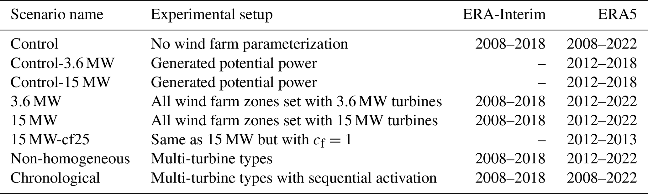
Different conceptual wind farm scenarios were designed, as summarized in Table 2. Two scenarios were set to estimate the maximum difference of the wake effects based on the available turbine data; both scenarios featured homogeneous turbine types across all wind farm areas but with the smallest and the largest available turbines' rated power, respectively, i.e. 3.6 and 15 MW. A 2-year simulation (15 MW-cf25), identical to the 15 MW simulation but with the turbulent kinetic energy coefficient reduced to one-quarter of its original value, as defined in Fitch et al. (2012) (c_f=0.25), was also performed. The non-homogeneous simulation consisted of non-homogeneous turbine types fitting the rated power for each wind farm as close as possible to the metadata information from the EMODnet dataset (Fig. 2). The Chronological simulation setup followed the same configuration as the non-homogeneous scenario, but the wind farms were activated in the year that each wind farm was commissioned, making this scenario more in line with real conditions in the past. For those wind farms that have no metadata on rated power, 15 MW turbines were assumed. Control scenarios with the wind farm parameterization switched off were used as reference simulations. They provide atmospheric data without accounting for wake effects. Control simulations (Control-3.6 MW and Control-15 MW) calculate the potential power output for the 3.6 and 15 MW turbine scenarios, representing the power that could be produced in the absence of wake effects. Except for the Control and Chronological simulations, all simulations assume a total installed capacity of 150 GW. To achieve this, the power density varies between simulations, with the number of turbines adjusted accordingly in each case.

Table 2 Wind farm scenarios and the simulated periods based on the availability of the forcing datasets.

Although the 3.6 MW scenario is unrealistic for future deployment, it provides a controlled baseline for comparison. By keeping all other factors constant, these scenarios isolate the effect of turbine size on energy yield, variability, and wake interactions. The comparison also helps to bound the range of possible outputs and highlights the benefits of technological scaling. Overall, this approach allows us to analyse the response of large-scale offshore wind power to turbine characteristics while maintaining methodological clarity.

To investigate the uncertainty in the generated power due to boundary conditions, simulations were conducted using two different driving datasets: ERA-Interim (Dee et al., 2011) and ERA5 (Hersbach et al., 2020) reanalysis data, covering the periods from 2008 to 2022 depending on the driving datasets (Table 2). ERA-5 and ERA-Interim datasets have spatial resolutions of approx. 0.7° (approx. 79 km) and 0.285° (about 37 km), respectively. To achieve the target resolution of 0.02° (approx. 2 km), a two-step offline nesting approach was adopted. COSMO5.0-clm15 (without wind farm parameterization) was used as the initial step to downscale reanalysis data to a resolution of 0.11° (approx. 12 km) (Geyer, 2014). Subsequently, this downscaled simulation served as driving conditions for the finer 0.02° resolution simulation conducted with COSMO6.0-clm, which includes the wind farm parameterization.

3.4 Atmospheric stability classification

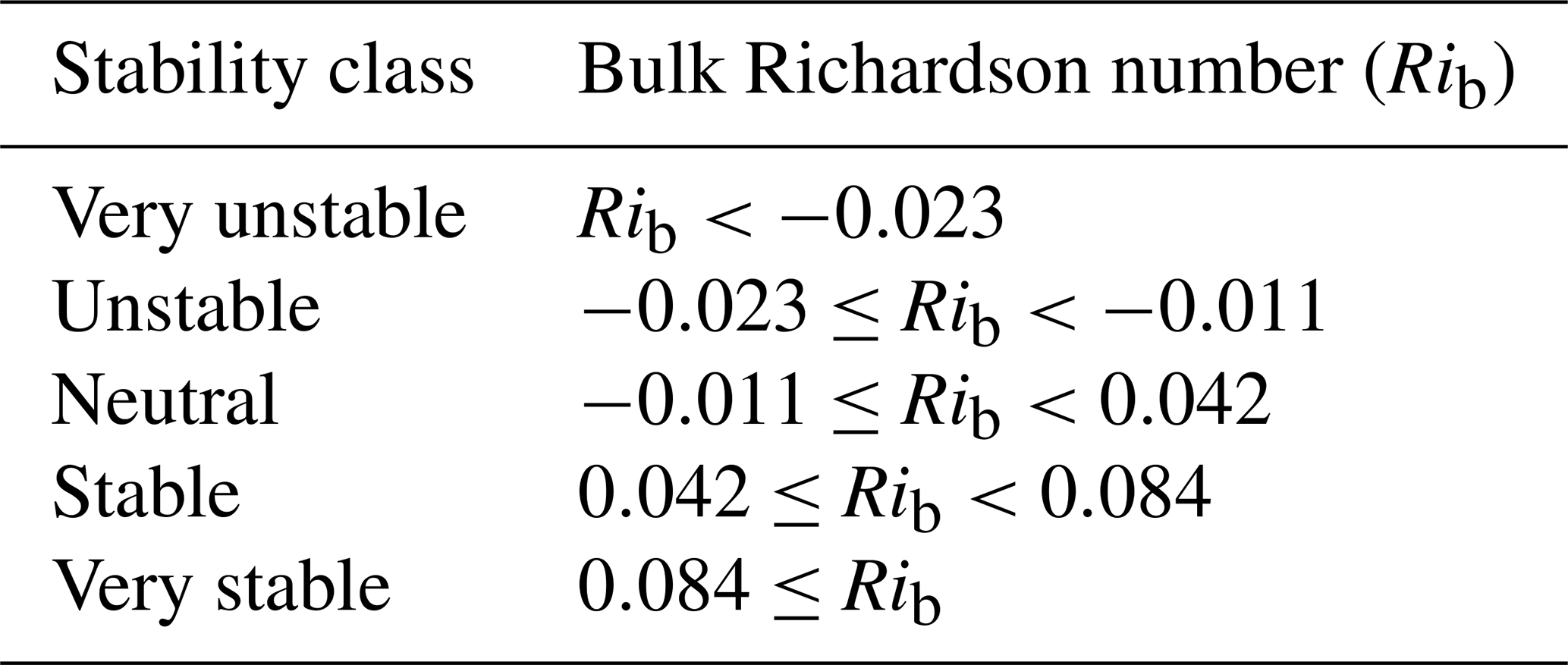
There are many methods to classify the atmospheric stability based on the altitude of the process of interest. Here, we follow the classification of the low atmosphere according to (Mohan, 1998), who established stability categories at turbulent boundary layer heights. This approach has been used in other studies related to wind energy research (Schneemann et al., 2020; Cantero et al., 2022). The calculated bulk Richardson number (Ri_b) at hub height is used to estimate the stability based on wind speed and mean virtual potential temperature. We use a simplified version from Mohan (1998), where weakly unstable, weakly stable, and neutral categories from the original classification are all merged in the neutral category (Table 3). The motivation arises from the fact that, in our case, the results from these three categories are similar and do not provide additional information. Nevertheless, the reassignment of those categories simplified the analysis.

Table 3 Bulk Richardson number thresholds used for atmospheric stability classification.

In our case, the bulk Richardson number (Ri_b) is calculated internally in the COSMO model (Doms et al., 2021) as

$$\begin{array}{}\text{(4)}& {\mathit{Ri}}_{\mathrm{b}}\left(z\right)={\displaystyle \frac{g\left[{\mathit{\theta }}_{\mathrm{v}}\right(z)-{\mathit{\theta }}_{\mathrm{v}}(z_{\mathrm{0}}\left)\right](z-z_{\mathrm{0}})}{{\mathit{\theta }}_{\mathrm{v}}\left(z\right)\left[\right(u\left(z\right)-u\left(z_{\mathrm{0}}\right){)}^{\mathrm{2}}+\left(v\right(z)-v(z_{\mathrm{0}}\left){)}^{\mathrm{2}}\right]}},\end{array}$$

where g is the acceleration due to gravity (m s⁻²), θ_v(z) is the virtual potential temperature (K) at height z, θ_v(z₀) is the virtual potential temperature (K) at the reference height z₀ (the aerodynamical roughness length), u(z) and v(z) are the respective zonal and meridional wind components (m s⁻¹) at height z, and u(z₀) and v(z₀) are the zonal and meridional wind components (m s⁻¹) at the reference height z₀. The heights z and z₀ are measured above ground level (m). This formulation provides a measure of atmospheric stability and is used in the COSMO model to diagnose the planetary boundary layer height (HPBL), typically by identifying the height at which Ri_b reaches a critical value.

4 Results

4.1 Wind speed validation

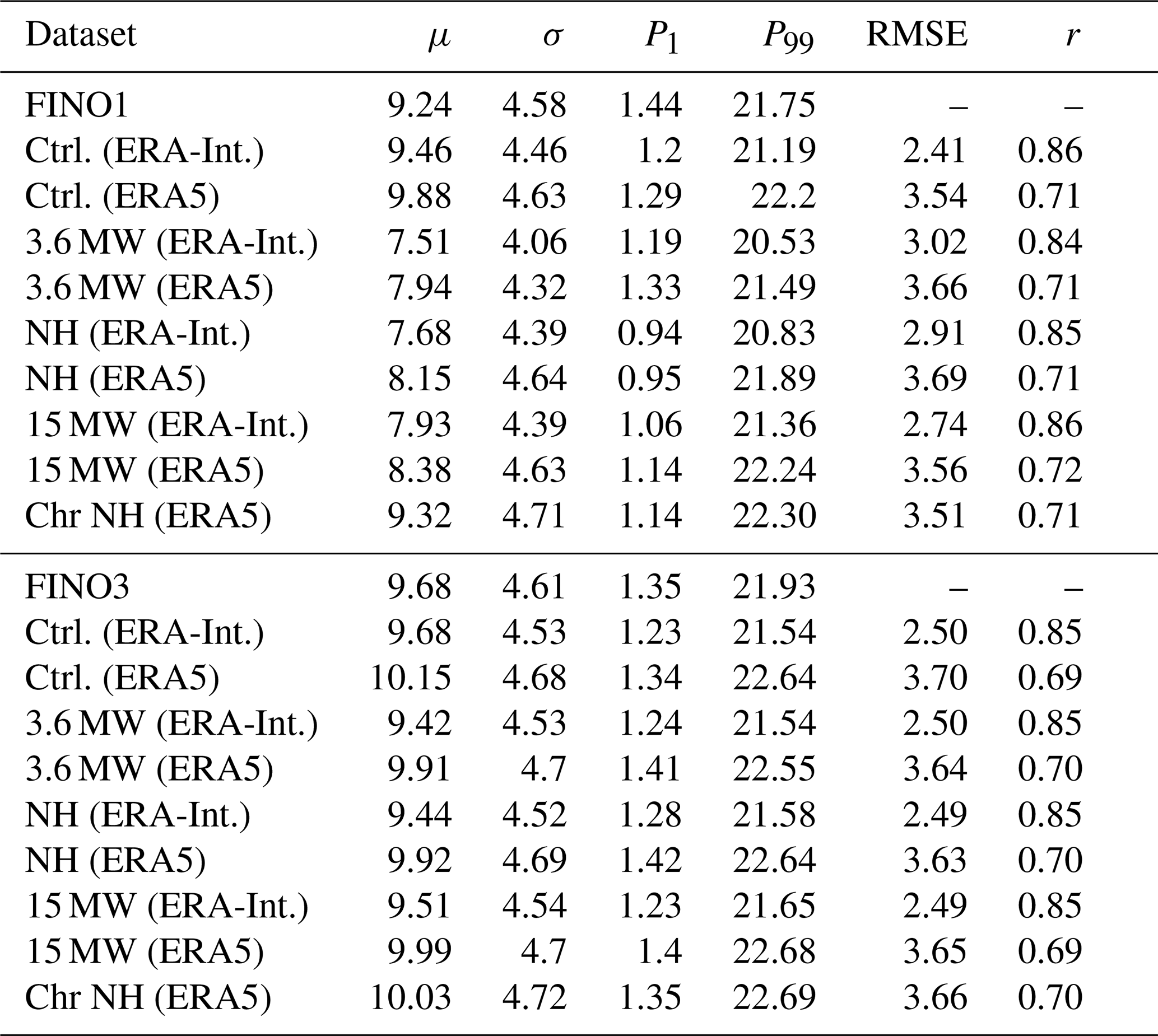
Wind speed observational data from the FINO1 and FINO3 platforms were compared with simulated wind speeds for the common period from 2012 to 2018. The time series at 90 m height for the grid box of each FINO platform location was extracted from the model grid and statistically compared (Table 4).

Table 4 Statistical comparison of simulated wind speeds at 90 m with FINO data. The columns correspond to the mean value (μ), standard deviation (σ), 1st and 99th percentiles (P₁ and P₉₉), root mean square error (RMSE), and Pearson correlation (r) for the period of 2012 to 2018. The top and bottom sections correspond to the comparison with FINO1 and FINO3, respectively. All units are in m s⁻¹ except for the unitless r value. All correlations were found to be statistically significant with p values below 0.01.

The FINO1 platform is located inside a cluster of five wind farms, with distances to the platform ranging from 1.4 to 15 km. Within the comparison period, two wind farms were set into operation in 2015. The time series of FINO1 shows an increase in turbulence intensity and a reduction in wind speed after each of the nearby wind farms became operational (Pettas et al., 2021). In the entire period of FINO1, the yearly mean wind speed decreased by around 1 m s⁻¹ from 2004 to 2019, mainly attributed to the effect of the wind farm wakes (Ortensi et al., 2020).

Mean wind speed from the Control experiments forced with ERA-Interim and ERA5, in comparison with FINO1 data, overestimate the observed values by 0.22 and 0.64 m s⁻¹, respectively. A positive bias is expected, as the Control simulations do not include the wind farm parameterization and therefore do not account for wake effects. In contrast, for the scenario simulations – except for the Chronological case – all wind farms are considered operational throughout the entire simulated period. This includes all wind farms in the vicinity of the FINO1 cluster as well as those in the adjacent eastern cluster, which amplifies the effects of wake effects and leads to an additional wind speed reduction. This leads to a negative bias from −0.86 to −1.73 m s⁻¹ on those simulations. The Chronological simulation, which activates the wind farms near the FINO1 platform sequentially according to their actual commissioning years, reduces the mean wind speed bias to 0.08 m s⁻¹. This indicates that this approach is capable of more accurately representing the wind conditions at FINO1. A more detailed comparison of the temporal evolution is addressed in Sect. 4.2.

Similar to FINO1, FINO3 is located in the vicinity of three wind farms. Two of them began operating in 2015, and the third one in 2017. The Control simulation driven by ERA-Interim should show overestimations of the measured wind speed at the FINO3 location, given that FINO3 data are already under the influence of wind farm wakes. However, only the ERA5-driven simulations meet this expectation. A comparison with scenarios does not yield big differences. The same as in the FINO1 results, the results from the scenarios are influenced by the driving conditions used. Simulations driven with ERA5 not only consistently produce higher wind speeds than those driven with ERA-Interim (as shown by the average and 1st and 99th percentiles values in Table 4) but also show higher variability as described by the standard deviation values. The RMSE and Pearson correlation indicate that those higher speeds represent a larger deviation from measurements for both FINO platforms, suggesting that, in our case, the ERA-Interim forcing is more beneficial to represent wind speed at FINO stations. The correlation between time series from an observational station and model data can be explained by their spatial representation. Observational stations measure a single point, which is subject to high local variability. In contrast, a model grid box represents the average wind speed over an area of approx. 4 km². This spatial averaging smooths out local fluctuations, leading to lower correlations with point measurements.

The spatial variability of the simulated wind speed field was validated against ASCAT satellite-based data. In the comparison, we included not only the corresponding wind fields from both Control simulations but also from the reanalysis datasets and the in-between COSMO5.0 simulations (with 0.11° resolution) that were used to drive the high-resolution COSMO6.0 simulations. Due to the coarse resolution of the ASCAT dataset, near-coast areas with mixed land–sea regions were masked in all datasets, leaving only the open-sea wind field for comparison, as indicated by the shaded area in the North Sea in Fig. 2.

The yearly cycle of the 10 m wind speed over the North Sea is shown in Fig. 3. ERA5 and ERA-Interim climatologies underestimate the 10 m wind speed in general, with the largest bias during the winter months. COSMO simulations tend to correct this bias in the late winter months. Similar to the findings of the FINO analysis, ERA5 shows systematically higher wind speed values than ERA-Interim, which are inherited by the COSMO simulations. The differences between the model versions of COSMO-CLM 5.0 and 6.0 are smaller than the differences derived using different forcings. This indicates that the double nesting approach and the change of model version do not accumulate any errors due to model numerics in the results.

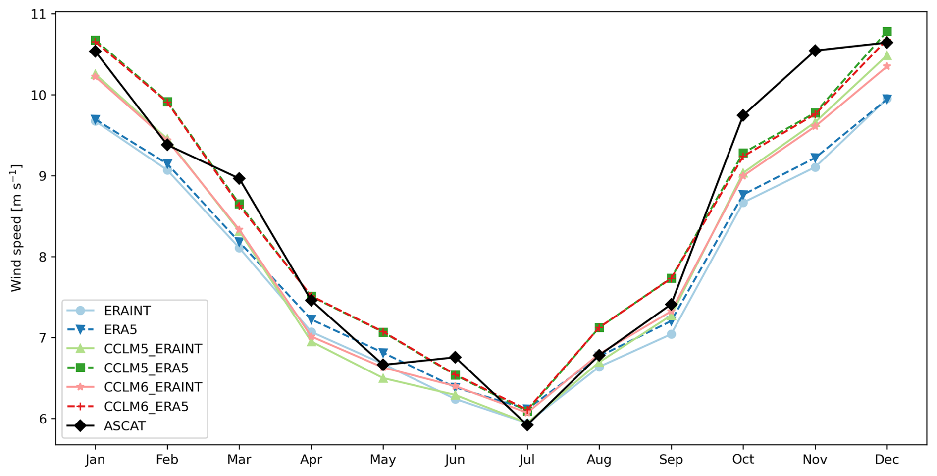
Figure 3 Yearly cycle for wind speed at 10 m height for the reanalysis data ERA-Interim and ERA5 (blue, solid, and dashed), the satellite data ASCAT (black), and the Control simulations done with the COSMO model versions 5 (green) and 6 (red) forced with both reanalysis datasets, averaged over the North Sea for the period from 2013 to 2018.

The spatial distribution of the RMSE of the 10 m wind speed based on daily values (see Fig. S1 in the Supplement) shows a larger error of around 1 m s⁻¹ in the eastern side of the North Sea for our Control simulations. Larger biases in the coastal areas in the reanalysis datasets are due to their low resolution, which mixes wind-related effects from land and ocean areas. Overall, the RMSE from ERA-Interim is smaller than in ERA5.

4.2 Reconstruction of wind speed at FINO1 platform

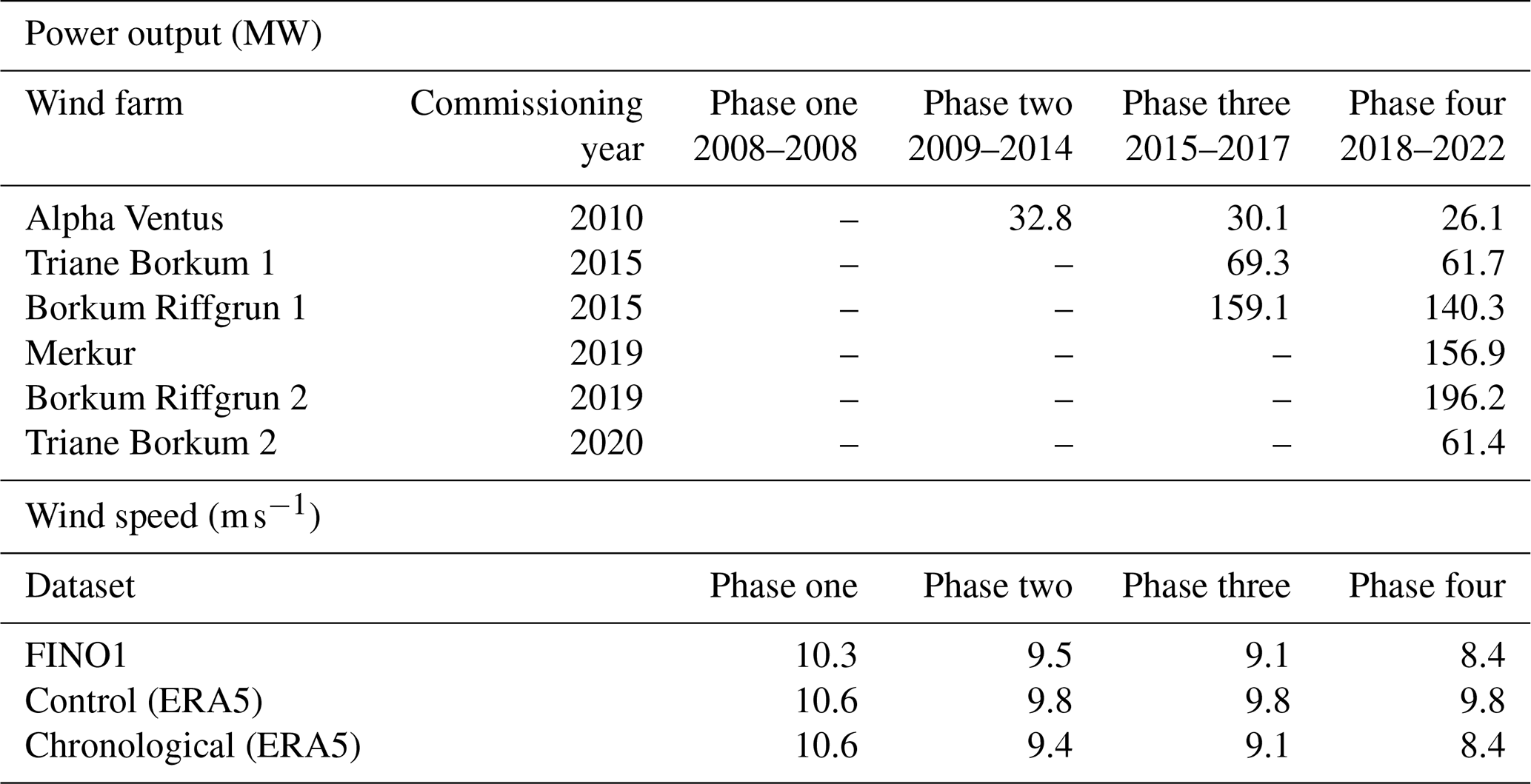
As new wind farms have been commissioned around the FINO1 platform over the years, wind speed measurements from the platform's onboard sensors provide an opportunity to quantify the impact of these developments on wind speed deficits and power generation in wind farm clusters. We compared observed wind speed with the Chronological simulation, in which wind farms were activated according to their commissioning year, with their specifications (area, turbine density, turbine height, rotor diameter, and rated power) adapted as closely as possible to reality based on EMODnet metadata. Figure 4 shows the wind speeds in the period 2008–2022 and the commissioning years of the wind farms in the vicinity of FINO1 (marked by small turbine symbols). The Control simulation represents the natural variability of wind speed without wake effects (orange curve), showing no clear trend during the analysed period. However, the negative trend in observed wind speed can only be attributed to the presence of the new wind farms (black curve). This negative trend is well captured in the Chronological simulation (red curve). The entire period was divided into four phases, with time boundaries close to the commissioning years of the wind farms. Table 5 summarizes the mean wind speed in each phase and the corresponding power generated by each wind farm. Wake effects contribute to a wind speed reduction of up to 16 % at the FINO1 platform by the end of the period, leading to an estimated 18 % decrease in power production at the Alpha Ventus wind farm.

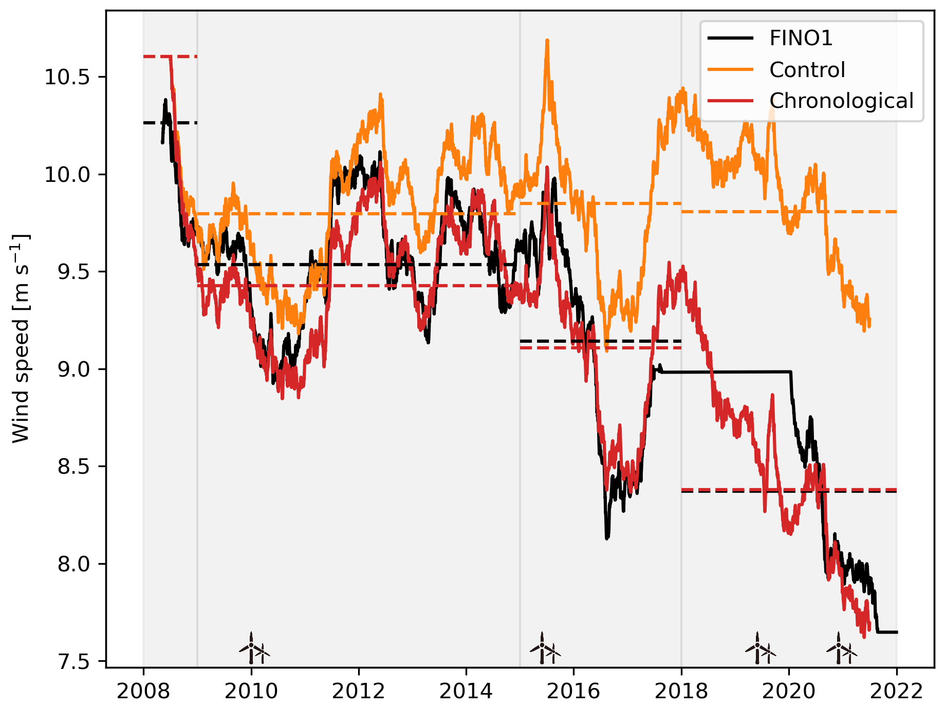
Figure 4 One year running mean time series for the mast-corrected observed wind speed at 91 m from the FINO1 platform (in black), simulated wind speed at 90 m for the Control simulation forced with ERA5 (in orange), and for the Chronological simulation (in red). Wind turbine symbols denote the commissioning year of wind farms near the FINO1 platform. Dashed lines indicate the mean values (Table 5) over each phase period, as defined by the vertical lines. Observational data are unavailable for the period 2018–2020.

Table 5 Simulated mean power output (MW) for several wind farms and wind speed (m s−1) at FINO1. The phases were defined by the commissioning years of the wind farms.

4.3 Case study of a wind farm cluster

4.3.1 Wake extension

The simulated wake effects are validated by using airborne measurements from the WIPAFF project. The observed wind speed data between 8:20 and 09:35 UTC on 10 September 2016 is compared with the simulated wind speed from the 3.6 MW scenario at 09:00 UTC on the same day. A low-pressure system centred over the Faroe Islands on that day favoured southwesterly winds at the German Bight and presented stable atmospheric conditions (Siedersleben et al., 2018) with an average wind speed of 7.86 m s⁻¹. The wake induced by the Amrumbank West, Nordsee Ost, and Windpark Meerwind SuedOst cluster was advected northwards with a prevailing wind direction of approx. 188° towards the Butendiek wind farm. The airborne data have a 10 ms temporal resolution. To compare with the simulation, the observed time series was smoothed by performing a running mean with a 3184 point window equivalent to a 2.2 km distance that matches the model spatial resolution. The model simulation is able to capture the wake effects as shown by wind speed anomalies – calculated as deviations from the respective dataset means – in Fig. 5. The downstream wind deficit closest to the cluster is about 1 m s⁻¹ in both (observed and simulated data) and decreases gradually northwards. The wind deficit extends up to 50 km, reaching the surrounding area of the Butendiek wind farm.

.

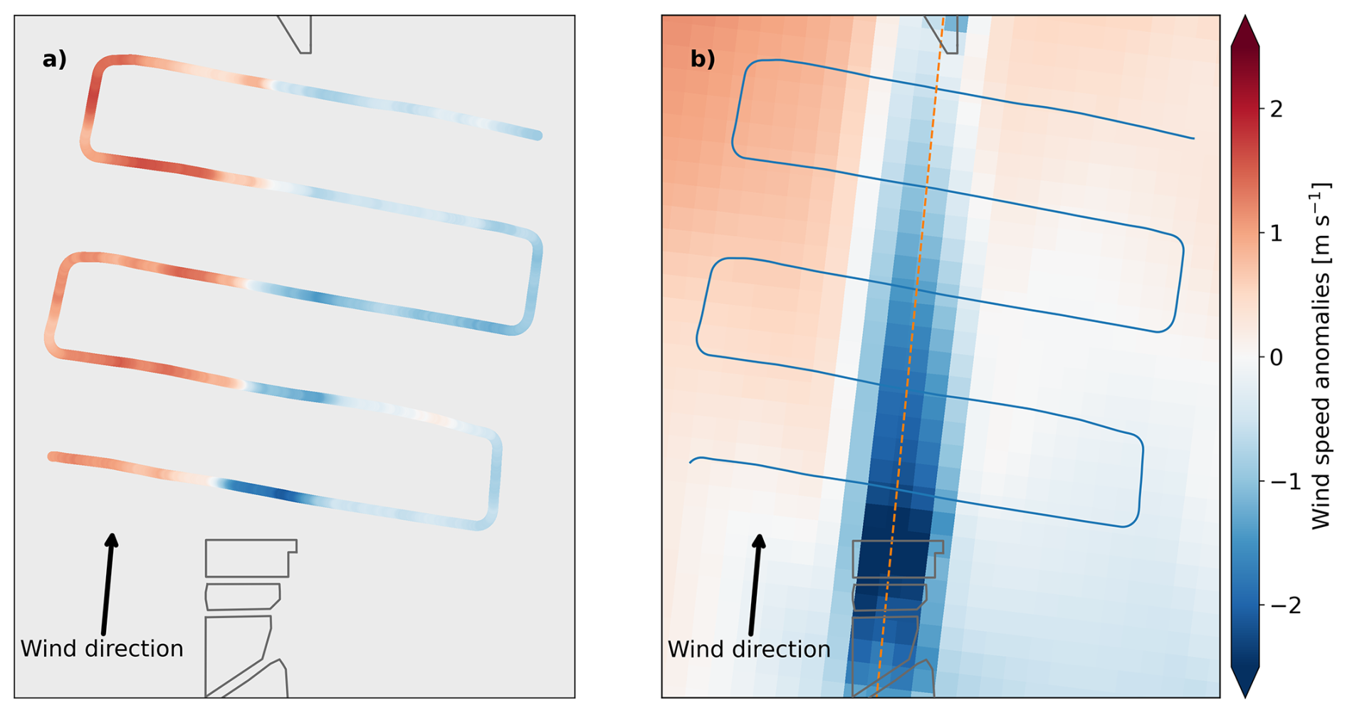
Figure 5 Wind speed anomalies, calculated as deviations from their respective dataset mean, for airborne observations dataset (left) and the 3.6 MW scenario simulation (right) in the downstream area of the wind farm cluster Amrumbank West, Meerwind Süd/Ost, and Nordsee Ost, along with the Butendiek wind farm in the north (in solid grey) on 10 September 2016 at 09:00 UTC. The dashed red line marks the cross-section depicted in Fig. 6.

The overall mean wind speed is underestimated by approx. 1 m s⁻¹, similar to results performed with the model version COSMO5.0-clm15 (Akhtar and Chatterjee, 2020). This bias is not related to the wake but to the general bias explained in the validation section (Sect. 4.1). The east-to-west gradient outside of the wake region is not well captured by the model, particularly on the eastern side. This bias seems to be not specific to COSMO6.0 only. A similar pattern has been reported in simulations using COSMO5.0-clm15 (Akhtar and Chatterjee, 2020) and WRF models (Siedersleben et al., 2018).

Figure 6 shows the wake influence on the vertical structure of the airflow across the section depicted in Fig. 5 (dashed red line). Wind farm areas are denoted by the space between the dashed grey lines, where the AW-MS-NO cluster is depicted on the left of each image, and Butendiek in the north is on the right side. The comparison refers to the difference between each scenario (3.6 MW, NH, and 15 MW) and the Control simulation. The largest wind deficits are located at the lee side of the cluster at altitudes between the hub height and the top of the rotor, with values up to −2.9 m s⁻¹ in the 3.6 MW scenario and up to −2.8 m s⁻¹ for the 15 MW one, which represents an approx. 45 % reduction with respect to the Control simulation. The difference between the scenarios is due to the presence of the largest number of turbines in the 3.6 MW scenario to achieve the same installed capacity as in the 15 MW scenario. The influence of the wake is not limited to the top of the rotor but reaches higher altitudes. For the smaller turbines of 3.6 MW, the deficits extend up to 100 m above the rotor to an altitude of 250 m. In the 15 MW scenario, the influence of the wake is extended only 50 m higher, to a height of approx. 300 m. The influence on higher altitudes of similar magnitudes has also been reported in previous studies (Akhtar et al., 2022; Siedersleben et al., 2020). The wake recovers as the distance from the cluster increases, starting from the upper layers where the wake influence is smaller. At the southern border of the Butendiek wind farm, the simulated wind deficit is limited to a height of 200 m in all the scenarios, and it accounts for about 10 % of wind speed reduction.

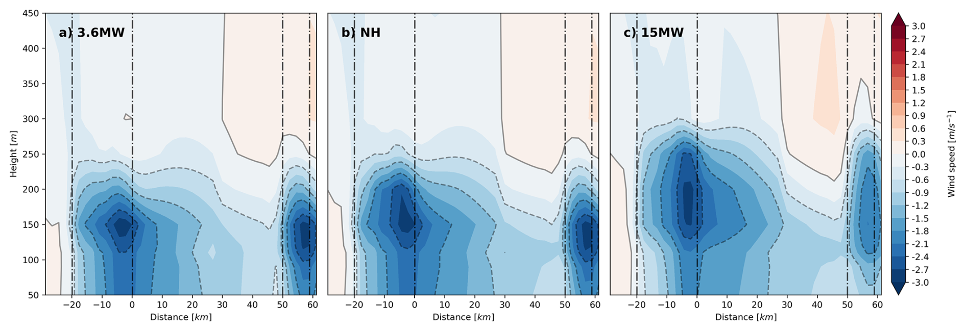
Figure 6 Wind speed differences due to wind farms (m s⁻¹) along the cross-section through the cluster and neighbour wind farm for three scenarios (3.6 MW, non-homogeneous rated capacity (NH), and 15 MW) compared to the reference simulation without wind farm parameterization for 10 September 2016. The airflow is directed from south to north (left to right in the image). The boundaries of the wind farm areas are indicated by vertical dash-dotted lines. Negative values are accentuated using dashed contour lines, and the zero contour is shown as a solid line.

4.3.2 Influence of atmospheric conditions on wake extension

It is well known that wake extension depends on atmospheric stability: unstable conditions enhance mixing and turbulence intensity, which increases the momentum transfer that diminishes the wind speed deficits (Platis et al., 2022), whereas during stable conditions, laminar flow advects unperturbed wind speed deficits, which increases the wake extension. Figure 7 shows composites of wind speed deficits based on different atmospheric conditions for the 15 MW scenario driven with ERA5 for September 2016. The constituents were filtered based on a wind direction criterion at the Amrumbank West wind farm (the northernmost wind farm in the cluster, located in the study case and indicated by a red box in Fig. 7). The wind direction should have a southerly component in the interval of ±5° centred at δ=188°, i.e. in the range between 183 and 193°. The constituents were then classified by their respective atmospheric stability condition at 120 m height (the closest height to 150 m hub height at which the model internally calculates the bulk Richardson number), according to Table 3. The figure shows the differences between the wind speed of the 15 MW scenario and the Control run. The vectors indicate the mean wind fields of both simulations (every 10 grid boxes). The mean wind speed at the Amrumbank West wind farm in all stability cases varies between 4.6 m s⁻¹ in the very unstable case and 6.4 m s⁻¹ in the neutral case; this implies that the wake extension is not necessarily coupled with the wind speed.

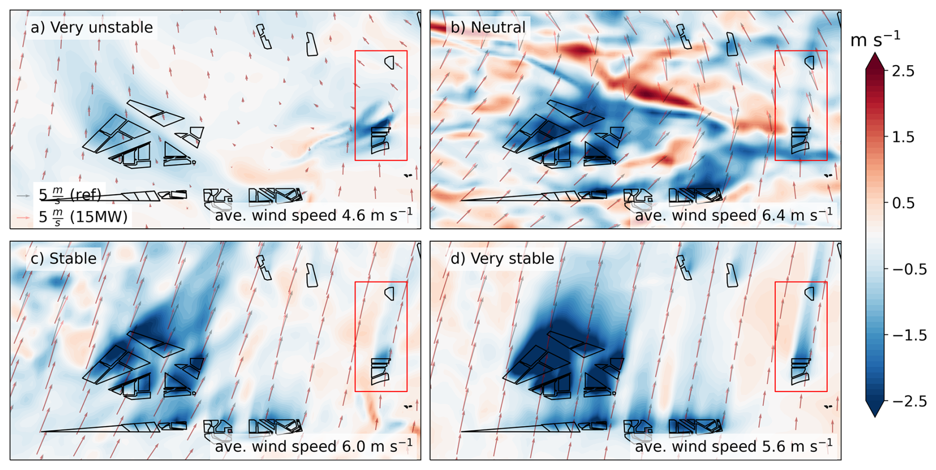
Figure 7 Composites of wind speed deficits (m s⁻¹) at 150 m height for southwesterly winds (183–193°) classified by their atmospheric stability at the German Bight area for September 2016. The wind direction is depicted by vectors in black for the reference simulation and in red for the 15 MW simulation. The wind farm cluster case study area (Fig. 5) is highlighted in the red box. The legends provide mean wind speed over the Amrumbank West wind farm.

The figure also shows a larger group of clusters situated in the west of the case study, where most of the wind farm sites are still planned (at the time of writing). A significant large wake influence among those clusters is not limited to only stable conditions but also under neutral conditions as a consequence of their respective proximity. The mean wind speed deficit in the large cluster accounts for −3.1 m s⁻¹ during neutral conditions and up to −4.0 m s⁻¹ under very stable conditions, which evidence that a large impact on power production for such clusters is expected.

4.4 Turbine power

Power production depends not only on wind speed but also on the atmospheric conditions and the influence of wakes from neighbouring wind farms. To quantify the effects of atmospheric stability on the power output, the generated power has been classified according to atmospheric stability. Figure 8 shows classified simulated power outputs for the 3.6 and 15 MW turbine scenarios at the Amrumbank West wind farm, along with statistical distributions of power and wind speed derived from hourly time series over the 11 year simulation period from 2008 to 2018 (in contrast to the composite analysis of a single month presented in the previous section).

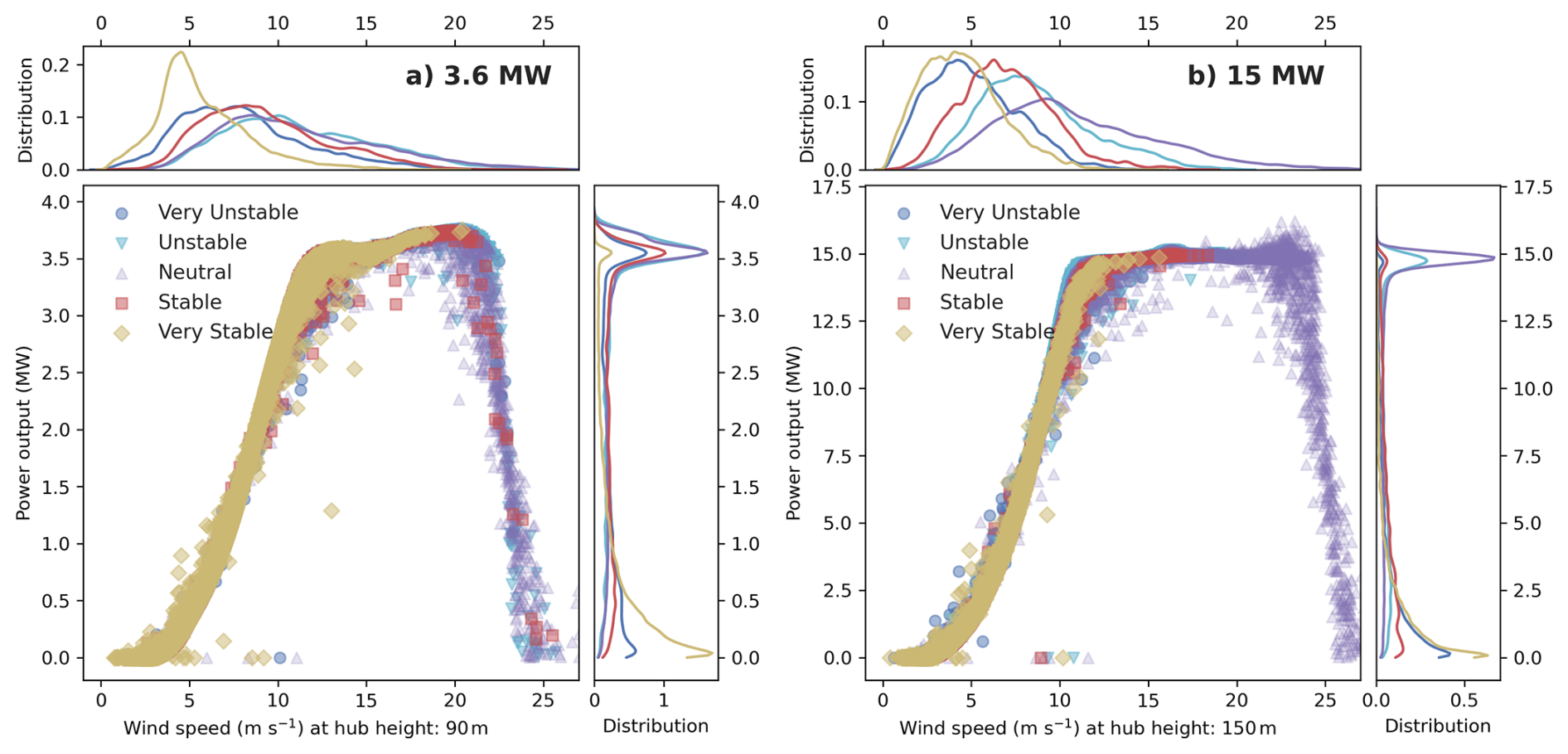
Figure 8 Model-simulated power curves based on hourly averaged data from 3.6 MW (a) and 15 MW (b) turbine types in the period from 2008 to 2018. The power output is classified by atmospheric stability conditions (in colours, plotted from very unstable to very stable, which causes overlaying symbols). Statistical distributions for the power output and wind speed are additionally depicted in the respective figure axes.

Wind speed values are more likely to occur within the turbine's partial load range (the wind speed interval between the cut-in – approx. 4 m s⁻¹ – and the rated power of approx. 11 m s⁻¹) for all stability cases, as shown in the wind distribution figures. Nevertheless, power distribution figures indicate that the optimal turbine power output (i.e. rated power) occurs more often under neutral, unstable, and very unstable conditions. Particularly relevant are the stable and very stable cases, under which relatively low wind speeds in the range from 4 to 11 m s⁻¹ may be further reduced if the turbine is under a wake influence, thereby diminishing the power production.

Simulated power values exceeding the turbine's rated power result from deviations in the provided tabulated data from the idealized power curve (see Fig. 1). The model does not account for turbine optimization above the cut-off wind speed (25 m s⁻¹); in such cases, the instantaneous power output is set to zero. However, the non-zero values above the cut-off wind speed in the figure arise from the calculation of the hourly average, where not all wind speed values within an hour necessarily exceed the cut-off threshold.

4.5 Uncertainty in wind farm power production

Atmospheric stability cases do not occur with the same frequency throughout the year. The analysis for monthly frequencies for atmospheric conditions at 90 and 150 m at wind farm sites in the North Sea from 2008 to 2018 show that neutral conditions prevail throughout the year (Fig. 9). Stable and very stable atmospheric conditions are more prevalent during summer and the transitional seasons, with very stable conditions occurring more frequently. Turbines with a hub height of 150 m experience a different wind regime, characterized by more frequent stable and very stable conditions compared to turbines at 90 m hub height. This is due to reduced surface-driven turbulence and persistent temperature gradients at higher altitudes. Near the ground, friction and solar heating generate turbulence and mixing, but these effects weaken with height. In Fig, 3, the mean wind speed is at its lowest during summer months; therefore, the combination of low wind speed and reduced turbulence is more likely to induce larger power losses as a consequence of the wake effects at this time of the year.

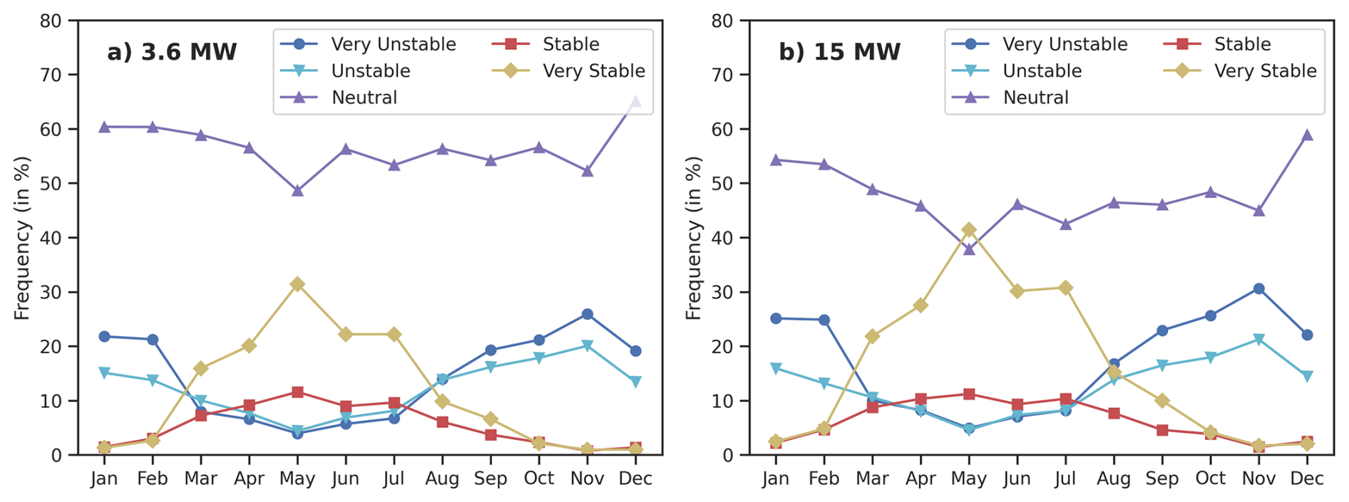
Figure 9 Yearly cycle of occurrences for different atmospheric conditions at the Amrumbank West wind farm in the simulations: (a) at 90 m height for the 3.6 MW scenario and (b) at 150 m height for the 15 MW scenario in the period from 2008 to 2018.

Figure 10 shows the annual distribution of power output for four simulations, the two scenarios (3.6 and 15 MW) each driven with ERA5 and ERA-Interim datasets. The yearly cycle of power output closely follows the seasonal pattern of wind speed (see Fig. 3). Nevertheless, two main features can be highlighted. First, simulations driven with ERA5 boundary conditions produce higher power output than those driven with ERA-Interim. This is a consequence of the higher wind speeds in the ERA5 dataset, as shown in the validation analysis (Sect. 4.1). The yearly mean wind speed is about 0.11 m s⁻¹ higher in ERA5 than in ERA-Interim. This corresponds to an annual power difference of approx. 4 GW more in ERA5 (2.5 % of the 150 GW (total) installed capacity, hereafter w.r.t. 150 GW of installed capacity). Second, by design, the wind farms in each scenario were set to have the same total installed capacity regardless of the turbine type. Nonetheless, Fig. 10 shows that the 15 MW scenario has a higher power output than the 3.6 MW one. The difference in annual power attributable to the turbine type is approx. 11 GW, corresponding to 7.5 % of the total installed capacity. Two main factors explain this last difference. First, to achieve the same installed capacity, the 3.6 MW scenario requires a higher turbine density than the 15 MW one. The denser layout amplifies wake effects, thereby reducing power output. Second, the 15 MW scenario includes larger turbines – with higher hub heights and larger rotor diameters – that operate in a wind regime with higher wind speeds, leading to increased power output.

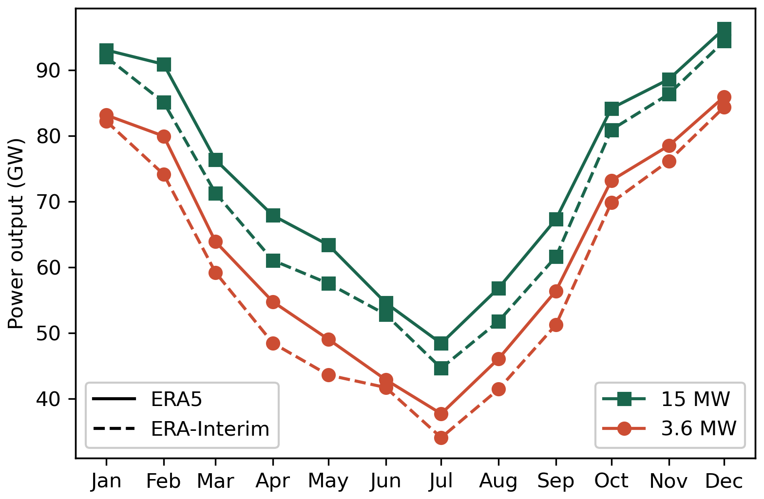
Figure 10 Yearly cycle for simulated power output (GW) from all wind farms in the North Sea for the period 2012–2018 for the two scenarios (3.6 and 15 MW, in green and orange, respectively), driven by ERA5 and ERA-Interim forcing datasets, represented by solid and dashed lines, respectively.

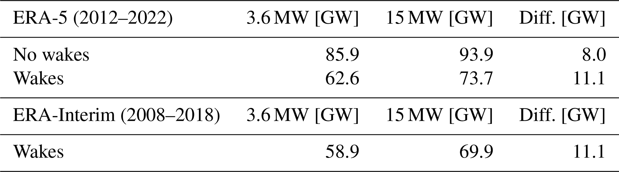
To isolate the individual impacts of turbine density and turbine sizes, we conducted two additional ERA5-driven simulations for the 3.6 and 15 MW scenarios. In these simulations, power output was calculated by the model under unperturbed flow, achieved by neglecting the contributions from the momentum sink and TKE source terms. Table 6 summarizes the annual power output over the North Sea with and without wake effects. Under unperturbed flow, the difference in turbine size accounts for approx. 8 GW (5.3 % w.r.t. 150 GW), whereas the remaining 3 GW (2.2 % w.r.t. 150 GW) is attributed to difference in wake effects derived of the turbine type.

Table 6 Simulated mean annual power output (GW) for the North Sea region (see Fig. 2) in the 3.6 and 15 MW scenarios, driven by ERA-5 and ERA-Interim boundary conditions. The annual mean wind speed is presented both including wake effects and under unperturbed flow (the latter only for ERA5-driven simulations). Averages correspond to 2012–2022 for ERA5-driven simulations and 2008–2018 for ERA-Interim-driven simulations.

The load factor of a wind farm, also known as the capacity factor, is defined as the ratio of the power output to the installed capacity. Table 7 shows the averaged load factor of all simulated wind farms in the North Sea with a total installed capacity of 150 GW for each of the scenarios driven by the ERA5 dataset. Wind conditions throughout the year limit the produced power to a fraction of 0.57 and 0.61 of the installed capacity for the 3.6 and 15 MW scenarios, respectively. By including the wake effects, in the 3.6 MW scenario, the load factor is reduced further to 0.42. This is consistent with reported load factors in the range of 0.23 to 0.52, with a mean value of 0.35 for the US and North Sea regions (Cassa, 2024; Smith, 2024). The discrepancy between the value in the 3.6 MW simulation and the reported mean values in existing literature may be partially ascribed to the control and management of power output in real wind farms. Turbine shutdowns encompass actions such as the regulation of power output for adaptation to real-time electricity demand, maintenance, and equipment upgrades, among others. These actions, which are difficult to assess due to the large unpredictability and the lack of public data, are not integrated into the model.

Table 7 Similar to Table 6 but for mean load factors, assuming a total installed capacity of 150 GW.

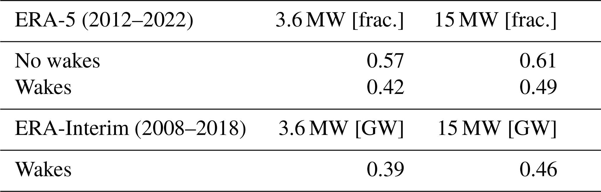
However, by examining the difference between the 3.6 and 15 MW scenarios, the turbine-type upgrade leads to an increment of the averaged load factor from 0.42 to 0.49, respectively. This represents an increase in power output by 7 percentage points (with a capacity of approx. 5 MW km⁻²). This result stands in the range of recently reported increments of 2 to 3 percentage points in Akhtar et al. (2024) (with a capacity of approx. 5 MW km⁻²) and 8.7 percentage points in Borgers et al. (2024) between 5 and 15 MW scenarios using COSMO5.0-clm15 version (with capacity densities from 3.5 to 10 MW km⁻²). Under ERA-Interim boundary simulations, the equivalent load factors become 0.39 and 0.46 for the 3.6 and 15 MW scenarios, respectively.

4.6 Effects of C_TKE correction on power output

Previous studies have shown that the original parameterization of Fitch et al. (2012) overestimates TKE by 50 % to 230 % compared with LESs (Abkar and Porté-Agel, 2015; Pan and Archer, 2018; Archer et al., 2020; García-Santiago et al., 2024). To address this, Archer et al. (2020) proposed reducing the C_TKE coefficient to one-quarter of its original value (i.e. c_f=0.25). This reduction converts less energy into turbulence, thereby decreasing mixing and increasing the relative contribution of undisturbed mean wind. Consequently, wake recovery is slower, wakes persist over longer distances, and downstream turbines experience lower wind speeds, leading to a decrease in simulated power output.

Table 8 Monthly mean values of power output (GW), wind speed (m s⁻¹), and TKE (m² s⁻²) at hub height (150 m) for 2012–2013 from the 15 MW and 15 MW-cf25 simulations. Negative relative differences (%) denote reductions in variable values of 15 MW-cf25 simulation relative to 15 MW simulation.

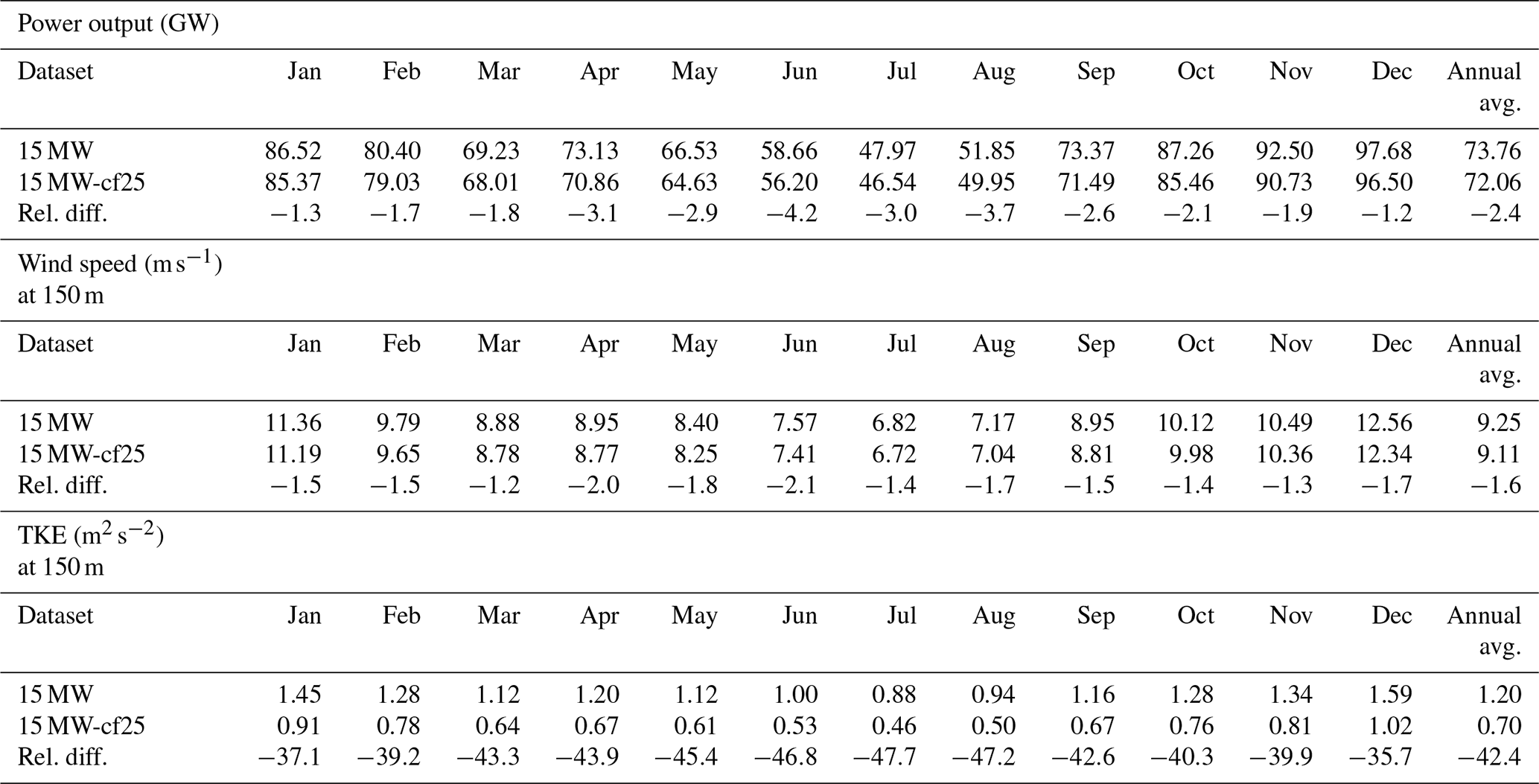
We selected the years 2012 and 2013 from the 15 MW simulation as a test bed to evaluate the impact of reducing the c_f coefficient to 0.25, using an otherwise identical setup (denoted as 15 MW-cf25). The 15 MW-cf25 simulation shows a mean power output reduction of approx. 2 % across all wind farm areas, lowering the annual mean output from 73.8 GW in the 15 MW simulation to 72.1 GW in 15 MW-cf25. This corresponds to a 1.1 percentage point reduction in the overall capacity factor relative to the 150 GW of installed capacity. However, the decrease is not evenly distributed throughout the year (Table 8). Although power output is higher in winter than in summer, consistent with wind speed climatologies, the relative difference is larger in summer. This behaviour can be explained by the relationship between mean wind speeds (Table 8) and the power curve of the 15 MW turbine (Fig. 8b). In winter, mean wind speed typically exceeds the threshold of approx. 11 m s⁻¹ at which the turbine reaches its rated power, so small decreases in wind speed have little effect on the power output. In summer, however, mean wind speed often remains below this threshold, meaning that even minor reductions directly reduce power output, leading to larger absolute and relative differences. For TKE, the mean reduction amounts to approx. 42 %.

5 Conclusions

The wind farm parameterization of Fitch et al. (2012) was implemented in the regional climate model COSMO6.0-clm, including the calculation of power output. The model now also incorporates wind farm metadata and multiple turbine types, allowing flexible scenario design. This enhancement enables the inclusion of different turbine types and densities in the same simulation, facilitating the creation of more realistic wind farm scenarios.

Similar to the previous model version, COSMO5.0-clm15, the wind field is simulated accurately, as confirmed by comparisons with station and satellite observations. This represents an improvement on the wind speed values from the reanalysis products ERA-Interim and ERA5, which tend to underestimate wind speeds due to their coarser resolution, particularly in coastal areas where larger errors are typically observed. The model reasonably captures the vertical structure and extent of the wake produced by the wind farms, considering the resolution and scale of the mesoscale model.

It is well known that atmospheric flow with stable conditions enhances the wake extension by advecting the wind deficits over longer distances, with a potential impact on neighbouring wind farms. Our atmospheric stability analysis shows that future planned wind farms close to large neighbouring clusters can still be subject to wake effects in neutral or unstable conditions, even when the wake recovery is expected to be faster under turbulent conditions.

From the power analysis assessment, we found that combined uncertainty from driving conditions and different turbine-type scenarios amounts to about 15 GW (10 % of the total installed capacity, or 150 GW), with driving conditions contributing 4 GW (2.5 %) and turbine-type differences, 11 GW (7.5 %). Of the latter, turbine size accounts for 8 GW (5.3 %) and wake interactions for 3 GW (2.2 %). Upgrading from 3.6 GW to 15 GW turbines substantially increases average load factors and power output, highlighting the fact that turbine size is an important factor for offshore wind power uncertainty in the North Sea, with the observed increase broadly consistent with ranges reported in existing offshore wind farm studies.

A sensitivity experiment in which the C_TKE coefficient has been reduced to one-quarter of its original value, as suggested by Archer et al. (2020), led to decrease in TKE production at hub height by 0.5 m² s⁻², lowering wind speed by 0.2 m s⁻¹ (due to wake recovery losses) and power output by approx. 2 GW (about 1 % of total installed capacity).

We emphasize that the uncertainty sources examined here represent only a subset of the broader uncertainty space associated with offshore wind power estimation, as additional uncertainties exist from technical factors like turbine geometry, layout, and performance characteristics; from atmospheric processes across multiple scales, such as wind profile representation, atmospheric stability, small-scale turbulence, and atmospheric dynamics; and from model-related aspects, including turbulence parameterization, spatial and temporal resolution, structural differences among modelling approaches, and the representation of interactions between neighbouring wind farms inside the model. Consequently, more detailed and refined investigations will be necessary to fully characterize these effects. Nonetheless, given that power output values are commonly employed to assess economic and environmental impacts, as well as to guide energy policies and planning decisions, we suggest that these uncertainties be explicitly considered in both scientific analyses and decision-making processes.