Damage identification on a large-scale wind turbine rotor blade using sample-based deterministic model updating

Wind turbine rotor blades are among the most critical components of wind turbines, with their structural integrity directly affecting reliability, lifetime, and maintenance costs. Reliable damage identification is therefore essential for structural health monitoring (SHM) strategies in wind energy applications. In this context, the updating of numerical models represents an established method for vibration-based non-destructive damage identification, including damage detection, localization, and quantification. Naturally, the model-updating process is affected by different sources of uncertainty. On the one hand, the numerical model always represents an idealization that introduces unavoidable discrepancies between its basic assumptions and reality. On the other hand, the measurement data and identified modal parameters, typically serving as damage-sensitive features, are subject to uncertainty. Despite extensive research on uncertainty quantification and propagation in model updating, comparative studies of model-updating procedures applied to large-scale structures, particularly wind turbine rotor blades, remain scarce. Moreover, the level of model fidelity and the impact of different design variable configurations associated with the selected numerical model are seldom examined in the context of model updating, typically formulated as an optimization procedure.

This study addresses this gap by systematically evaluating how model fidelity and design variable parameterization influence the model-updating results while considering input uncertainty associated with the measurement data and identification process. The investigations are conducted using measurement data from a 31 m rotor blade subjected to edgewise fatigue loading.

A comparison of the results shows that all design variable configurations yield consistent results, confirming the robustness of the presented model-updating procedures. Model fidelity, however, strongly influences the outcomes, with higher accuracy and detail leading to distinctly improved damage identification.

1 Introduction

The structural integrity of wind turbine rotor blades directly affects the operational reliability, energy yield, service lifetime, and maintenance costs of entire wind farms (Hau, 2013; Civera and Surace, 2022). The blades are typically highly loaded and critical to the overall design of the turbine (Kong et al., 2023). With the continuous upscaling of turbine and blade size, rotor blades are increasingly exposed to fatigue loads, making them susceptible to damage initiation and crack propagation. Algolfat et al. (2023) give an overview of common damage scenarios for wind turbine rotor blades. In this context, manufacturing defects were estimated to account for approximately 50 % of all blade damages (Civera and Surace, 2022). It is pointed out that such types of damage can lead to failure or breakdown of the wind turbines as they increase the level of vibrations and impose additional dynamic loads (Algolfat et al., 2023). Consequently, reliable identification and characterization of blade damage are essential for effective structural health monitoring (SHM) strategies in wind energy applications (Yang et al., 2017; Kaewniam et al., 2022). Haseeb and Krawczuk (2026) give a comprehensive review of SHM techniques applied for wind turbine rotor blades along with causes and types of blade damage.

Within an SHM framework, the basic assumption is that damage, defined as degradation of mechanical properties (Worden et al., 2007), causes detectable changes in structural dynamic behaviors (Mottershead and Friswell, 1993). Hence, to enable damage identification, including detection, localization, and quantification, vibration measurement data need to be acquired for at least two different states of the considered structure (Friswell, 2007), meaning a reference state and an analysis (i.e., target) state. A variety of different SHM methods based on various damage-sensitive features have been developed and applied to date (Avci et al., 2021). Such approaches are of vital importance when seeking to maintain the safety and integrity of the structures under consideration (Brownjohn, 2007; Fan and Qiao, 2011). Among them, the updating of numerical models represents an established vibration-based non-destructive damage identification technique (Das et al., 2016; Ereiz et al., 2022), which is also employed within this work. Due to its methodology, the model-updating process is affected by two major sources of uncertainty – associated with the model and the measurement data – as clearly pointed out by Simoen et al. (2015).

One source of uncertainty arises from the numerical model employed in the updating procedure. Depending on its level of fidelity, in terms of the chosen finite-element (FE) type, the numerical model represents a more or less simplified version of the structure under consideration and, by definition, always remains an idealization. Consequently, a certain level of discrepancy between the model predictions and the corresponding characteristics identified from the measurement data is inevitable (Mottershead et al., 2011). Christodoulou et al. (2008), for example, use multi-objective model updating to demonstrate that higher-fidelity models lead to better predictions, resulting in reduced variability of the Pareto optimal solutions. Their investigations were performed using experimental data from a 2.4 m high three-story steel structure. With regard to the modeling of (wind turbine) rotor blades, extensive research has been conducted on the comparison of numerical models based on different FE types and, thus, with varying levels of model fidelity (Lake and Nixon, 1988; Volovoi et al., 2001; Peeters et al., 2018; de Almeida et al., 2025). However, comparative analyses of model-updating procedures applied to large-scale structures, especially to wind turbine rotor blades, using different numerical models and associated design variable configurations remain scarce. Mostly, model-updating procedures applied to small- or large-scale wind turbine rotor blades utilize FE beam models (Noever-Castelos et al., 2022; Turnbull and Omenzetter, 2024). Chetan et al. (2021), for example, propose a multi-fidelity digital twin model for the simulation of a 21 m sub-scale wind turbine rotor blade but perform the actual updating of the mass and stiffness distributions using an Euler–Bernoulli beam model. Moreover, the application of detailed shell-based models for model updating, allowing for damage identification along the blade span and chord, is rarely published. Knebusch et al. (2020) applied a gradient-based model-updating procedure to a 20 m rotor blade using a detailed shell model. However, the design variables were mapped directly to material properties of so-called predefined design fields, representing FE groups. While this is a common approach to keep the number of design variables low (Levin and Lieven, 1998), it is dependent on a prior grouping of FEs and can result in undesired oscillatory stiffness distributions when an unconstrained formulation is used.

Another source of uncertainty is the measurement data. Due to the unavoidable spatial sparsity and noisiness of sensor signals and possible imperfections in the measurement equipment, measured data always contain uncertainty, which can merely be minimized but never fully eliminated (Link, 1999). In addition to the uncertainty contained in the raw measurement data, further uncertainty is introduced during the subsequent signal processing and identification of modal characteristics of the physical structure (Friswell and Mottershead, 1995), which is referred to as identification uncertainty. In recent years, numerous studies have investigated uncertainty quantification and propagation in model updating, employing methods such as Bayesian inference (Bi et al., 2021), interval approaches and fuzzy logic (Faes and Moens, 2020), and the sample-based deterministic model-updating (SDMU) approach recently introduced by the authors (Wolniak et al., 2025a). However, the primary focus of these works has typically been on methodological development rather than on large-scale experimental validation.

Within this work, the described input uncertainty sources inherent to the model-updating process are systematically examined and addressed using a 31 m laboratory wind turbine rotor blade subjected to edgewise fatigue loading. The rotor blade was instrumented with accelerometers to monitor its gradual stiffness degradation due to the fatigue loading, ultimately leading to crack growth across the leading edge at approximately 8 m distance from the blade root. The measured acceleration time series along with the corresponding modal properties identified from the measurement data using Bayesian operational modal analysis (BayOMA) (Au et al., 2013; Au, 2017) are published in an open-access repository (Wolniak et al., 2025b) alongside this paper. This unique experimental dataset provides a basis for monitoring the gradual stiffness degradation of a large-scale laboratory rotor blade tested under edgewise fatigue loading.

An outstanding feature of this rotor blade fatigue test was the complete documentation of the manufacturing process, accompanied by detailed material and geometry data. This extensive information enabled the development of two numerical models, i.e., a beam model and a shell model, with differing levels of fidelity, both of which are employed and compared within the model-updating procedure(s). Consequently, different design variable configurations are introduced and applied, as their selection depends not only on the purpose of model updating but also on the specific numerical model used in the updating process, including its element type and geometry. In this work, all presented design variable configurations define a one- or two-dimensional damage distribution function used to alter the stiffness properties of the respective numerical model. This definition ensures a smooth, realistic stiffness distribution and is independent of the FE mesh resolution and of prior assumptions about the defect location while requiring only a few design variables. Moreover, it can cover a wide range of damage scenarios, from highly localized defects affecting only a few FEs to one FE to a smoothly distributed stiffness degradation over an extended region. As in all related studies (Fan and Qiao, 2011; Simoen et al., 2015; Ereiz et al., 2022), this work also uses the discrepancies between simulated and identified modal properties as updating objectives. In particular, the eigenfrequencies and eigenmodes of the large-scale rotor blade are utilized in this work. To avoid the need for weighting factors, multi-objective optimization is applied (Christodoulou et al., 2008). In addition, both objective functions are formulated in relative terms, taking into account a possible constant discrepancy between the simulated and identified responses for both the analysis and the reference states. To account for the identification uncertainty associated with the modal properties identified from the measurement data, the SDMU approach is utilized (Wolniak et al., 2025a). This approach is motivated by a separation of the incorporation of this particular input uncertainty and the model-updating procedure itself, resulting in an approach that is fully adaptable to the specific problem at hand. In this work, an SDMU realization that delivers fully deterministic and reproducible results is applied.

The following key points summarize the fundamental aspects of this study:

• publication of a unique experimental dataset along with identified modal properties, providing a basis for monitoring the stiffness degradation of a large-scale rotor blade tested under edgewise fatigue loading;

• application of a beam and shell model within the model-updating process to compare different levels of fidelity;

• application of different design variable configurations tailored to the respective numerical models utilized.

The combination of a unique large-scale rotor blade fatigue test, the systematic model updating across the gradual stiffness degradation of the rotor blade, and the comparative evaluation of numerical models and associated design variable configurations of different levels of fidelity constitutes a novel contribution in the context of SHM for wind turbine rotor blades. The results demonstrate the methodological robustness of the proposed model-updating procedure, including the SDMU approach that considers and propagates input uncertainty, in this work associated with the measurement data and the subsequent modal parameter identification, and including the use of the one- and two-dimensional damage distribution functions parameterized by the different design variable configurations. Moreover, the findings of this work underline the importance of defining the analysis objective in advance, as the choice of the numerical model and the associated design variable parameterization is decisive in obtaining meaningful and reliable results.

2 Model updating

Typically, a model-updating problem is formulated inversely and treated as an optimization problem (Mottershead et al., 2011). An objective function is used to compare the structural dynamic behavior of the numerical model to a target state, and an optimization algorithm is used to find a model to match this target state by updating the selected design variables. Most often, this is achieved through stiffness or mass modifications (Friswell and Mottershead, 1995).

The utilized optimization algorithm is essentially designed to solve bounded and nonlinear optimization problems. This can be stated as

$$\begin{array}{}\text{(1)}& \mathrm{minimize}\mathit{\epsilon }\left(\mathit{x}\right)\mathrm{for}\mathit{\epsilon }\in {\mathbb{R}}^m,\mathit{x}\in {\mathbb{R}}^n,\end{array}$$

where ε is a vector-valued function consisting of m objective functions $\mathit{\epsilon }\left(\mathit{x}\right)=\left({\mathit{\epsilon }}_{\mathrm{1}}\left(\mathit{x}\right),{\mathit{\epsilon }}_{\mathrm{2}}\left(\mathit{x}\right),\mathrm{\dots },{\mathit{\epsilon }}_m\left(\mathit{x}\right)\right)$, and x is the n-dimensional vector of design variables. In this work, multi-objective optimization is applied, where the concept of Pareto dominance is followed (Marler and Arora, 2004). The space of the design variables is bounded by the volume of a hypercube

$$\begin{array}{}\text{(2)}& {\mathit{x}}_{\mathrm{lb}}\le \mathit{x}\le {\mathit{x}}_{\mathrm{ub}},\end{array}$$

where x_lb and x_ub are the lower and upper bounding vectors, respectively. For the optimization performed in this work, the optimization framework EngiO, introduced by Berger et al. (2021), is utilized.

From Eq. (1), it is clear that the optimization process and, thus, the quality of model-updating results depend on two key aspects: on the configuration of the design variables x on the one hand and, on the other hand, on the formulation of the objective function ε(x). In the following subsections, detailed information is given about the definitions used in this work.

2.1 Design variables

The determination of the design variables strongly depends on the purpose of model updating. Since the aim of this contribution is damage identification, specifically damage localization and quantification, the parameterization should be able to identify the geometric position of the damage and its intensity.

As damage mainly manifests itself as a change in stiffness, the general approach for most FE model-updating procedures with the aim of damage identification is to alter the stiffness properties of the model at hand (Friswell and Mottershead, 1995). This approach is also applied in this work. As no prior knowledge of the defect location is assumed, the updating of the stiffness properties of all N_el elements is performed, independent of the element type. This is implemented by adapting the initial Young's modulus E₀ of each FE with a corresponding scaling factor θ_k

$$\begin{array}{}\text{(3)}& E_{\mathit{\theta },k}=E_{\mathrm{0}}{\mathit{\theta }}_k\mathrm{with}k\in [\mathrm{1},N_{\mathrm{el}}].\end{array}$$

The stiffness scaling factors θ_k are calculated on the basis of the design variables. In this work, the design variables parameterize a so-called damage distribution function, previously introduced and applied by the authors (Wolniak et al., 2023). By formulating the mapping of the considered structural properties to the FEs using a distribution function, a smooth and realistic spatial distribution is ensured. As a result, the model-updating process is forced to focus on global structural dynamics instead of over-fitting local deviations. Moreover, the model-updating procedure is independent of the FE mesh resolution and of prior assumptions about the defect location while only needing a few design variables. However, applying the damage distribution in its current form restricts damage identification to only one damage position. In this work, a spatial Gaussian damage distribution function is considered based on the assumption that the damage roughly follows this type of distribution. In addition, this representation can cover a wide range of damage scenarios, from highly localized defects affecting only a few FEs to one FE to a smoothly distributed stiffness degradation over an extended region. Furthermore, the smooth spatial distribution of the damaged area leads to a comparatively smooth objective function, which, in turn, promotes faster and more stable convergence of the utilized optimization algorithm.

The determination of the design variables additionally depends on the specific model used in the updating procedure, as its element type and geometry inherently influence their configuration. In this work, two different numerical models of the large-scale rotor blade are considered, which necessitate at least two different design variable configurations. In the following subsections, firstly, the parameterization of a one-dimensional damage distribution function for the model updating using a rather simple beam model of the rotor blade is presented. This definition, based on three design variables, has already been introduced and successfully employed in several preceding publications (Bruns et al., 2019a, b; Wolniak et al., 2023), where deterministic model updating was performed on simulated and experimental application examples. In addition, in this work, the one-dimensional parameterization is extended by a fourth design variable, which independently adjusts the stiffness properties in the edgewise and flapwise directions of the rotor blade, allowing for a distinct consideration of both directions. Secondly, the parameterization of a two-dimensional damage distribution function for the model updating using a more detailed shell model of the rotor blade is introduced. This configuration is based on five design variables and allows for damage identification in the longitudinal direction and circumferential direction.

2.1.1 One-dimensional damage distribution function – three design variables

The one-dimensional damage distribution function is defined along a single control variable, specifically the length L of the beam model representing the rotor blade. It can be described by the three design variables,

$$\begin{array}{}\text{(4)}& {\mathit{x}}_{\mathrm{1}\mathrm{D}}={\left({\mathit{\mu }}_L{\mathit{\sigma }}_L{D}_{\mathrm{1}\mathrm{D}}\right)}^{\mathrm{T}}.\end{array}$$

In the design variable vector x_1D; μ_L represents the geometric position of the distribution function's center point along the length; σ_L represents the width of the spatial distribution, i.e., the extent of the damage; and D_1D represents the intensity of the damage. In this case, the damage intensity is defined as the area under the Gaussian-shaped spatial distribution function defined by μ_L and σ_L.

The calculation of the stiffness scaling factors θ_1D,k for each FE with a corresponding length l_k is based on the formulation of a probability density function $f\left(c_{L,k}\mid {\mathit{\mu }}_L,{\mathit{\sigma }}_L\right)$ calculated along the control variable c_L,k and truncated to the interval $\mathrm{0}\le c_{L,k}\le L$:

$$\begin{array}{}\text{(5)}& {\mathit{\theta }}_{\mathrm{1}\mathrm{D},k}=\mathrm{1}-D_{\mathrm{1}\mathrm{D}}L{\displaystyle \frac{f\left(c_{L,k}\mid {\mathit{\mu }}_L,{\mathit{\sigma }}_L\right)}{l_k}}\mathrm{with}k\in [\mathrm{1},N_{\mathrm{el}}].\end{array}$$

The stiffness scaling factors are evaluated at the center of each beam element length l_k. More detailed information regarding the one-dimensional damage distribution function parameterized by three design variables is given in Wolniak et al. (2023).

2.1.2 One-dimensional damage distribution function – four design variables

By introducing a fourth design variable, $\mathit{\lambda }\in [\mathrm{0},\mathrm{1}]$, the above-described one-dimensional damage distribution function is extended so that it can alter the stiffness properties in flapwise and edgewise directions separately. Therefore, instead of changing the initial Young's modulus E₀ of each FE, which alters each element stiffness altogether, the initial moments of inertia I_xx,0 and I_yy,0 in flapwise and edgewise directions and the initial moment of deviation I_xy,0 are updated separately from each other in an equivalent way to Eq. (3):

$$\begin{array}{}\text{(6)}& \begin{array}{rl}\left(\begin{array}{c}{I}_{xx,\mathit{\theta },k}\\ I_{yy,\mathit{\theta },k}\\ I_{xy,\mathit{\theta },k}\end{array}\right)& =\left(\begin{array}{c}{I}_{xx,\mathrm{0},k}\\ I_{yy,\mathrm{0},k}\\ I_{xy,\mathrm{0},k}\end{array}\right)\circ \left(\begin{array}{c}{\mathit{\theta }}_{xx,\mathrm{1}\mathrm{D},k}\\ {\mathit{\theta }}_{yy,\mathrm{1}\mathrm{D},k}\\ {\mathit{\theta }}_{xy,\mathrm{1}\mathrm{D},k}\end{array}\right)\\ & \mathrm{with}k\in [\mathrm{1},N_{\mathrm{el}}].\end{array}\end{array}$$

The calculation of the stiffness scaling factors θ_1D,k for each of the three moments of inertia follows a similar approach to Eq. (5), except that the damage intensity D_1D is scaled by different factors λ_xx, λ_yy, and λ_xy:

$$\begin{array}{}\text{(7)}& \begin{array}{rl}\left(\begin{array}{c}{\mathit{\theta }}_{xx,\mathrm{1}\mathrm{D},k}\\ {\mathit{\theta }}_{yy,\mathrm{1}\mathrm{D},k}\\ {\mathit{\theta }}_{xy,\mathrm{1}\mathrm{D},k}\end{array}\right)& =\mathrm{1}-D_{\mathrm{1}\mathrm{D}}\left(\begin{array}{c}{\mathit{\lambda }}_{xx}\\ {\mathit{\lambda }}_{yy}\\ {\mathit{\lambda }}_{xy}\end{array}\right)L{\displaystyle \frac{f\left(c_{L,k}\mid {\mathit{\mu }}_L,{\mathit{\sigma }}_L\right)}{l_k}}\\ & \mathrm{with}k\in [\mathrm{1},N_{\mathrm{el}}],\end{array}\end{array}$$

whereby these different factors are defined based on the fourth design variable λ:

$$\begin{array}{}\text{(8)}& \left(\begin{array}{c}{\mathit{\lambda }}_{xx}\\ {\mathit{\lambda }}_{yy}\\ {\mathit{\lambda }}_{xy}\end{array}\right)=\left(\begin{array}{c}\mathit{\lambda }\\ \mathrm{1}-\mathit{\lambda }\\ \sqrt{\mathit{\lambda }\left(\mathrm{1}-\mathit{\lambda }\right)}\end{array}\right)\mathrm{with}\mathit{\lambda }\in [\mathrm{0},\mathrm{1}].\end{array}$$

The presented formulation allows the single design variable λ to capture the trade-off between edgewise and flapwise stiffness. In addition, the total stiffness alteration applied in the different lateral directions of the structure remains proportional to the damage intensity D_1D, which is determined and adjusted by the employed optimization algorithm. Consequently, the progression of the model-updating procedure mirrors that of utilizing only three design variables (cf. Sect. 2.1.1), with the added ability to introduce damage separately in the two lateral directions.

For the calculation of the scaling factor λ_xy, it is assumed that the structural stiffness undergoes an affine transformation characterized by independent scaling along the two lateral axes (Timoshenko and Gere, 2012). This preserves the overall shape of the stiffness distribution while modifying its extents along the x (i.e., flapwise) and y (i.e., edgewise) axes. As a result, the scaling factor for the moment of deviation (also referred to as the product of inertia), I_xy, can be derived as the geometric mean of the scaling factors for I_xx and I_yy; i.e., ${\mathit{\lambda }}_{xy}=\sqrt{{\mathit{\lambda }}_{xx}{\mathit{\lambda }}_{yy}}=\sqrt{\mathit{\lambda }\left(\mathrm{1}-\mathit{\lambda }\right)}$.

2.1.3 Two-dimensional damage distribution function – five design variables

Using the shell model as a representation of the rotor blade, a parameterization of the damage distribution function along a single control variable, i.e., the length L of the rotor blade, is no longer sufficient. The parameterization has to be extended to a second control variable, meaning the perimeter P of the rotor blade. As a result, a two-dimensional damage distribution function is defined on the surface of the shell model, and the design variable vector describing this two-dimensional damage distribution function is extended to five entries:

$$\begin{array}{}\text{(9)}& {\mathit{x}}_{\mathrm{2}\mathrm{D}}={\left({\mathit{\mu }}_L{\mathit{\sigma }}_L{\mathit{\mu }}_P{\mathit{\sigma }}_P{D}_{\mathrm{2}\mathrm{D}}\right)}^{\mathrm{T}}.\end{array}$$

As the damage distribution function is now bell-shaped, its center point is described by the two geometric positions μ_L and μ_P along the length and the perimeter of the rotor blade, respectively:

$$\begin{array}{}\text{(10)}& {\mathit{\mu }}_{\mathrm{2}\mathrm{D}}=\left(\begin{array}{c}{\mathit{\mu }}_L\\ {\mathit{\mu }}_P\end{array}\right).\end{array}$$

As the blade's perimeter changes along its length, the design variable μ_P is normalized to values between $-\mathrm{0.5}<{\mathit{\mu }}_P\le \mathrm{0.5}$, whereby the value 0 corresponds to the leading edge (LE) and the values −0.5 and 0.5 correspond to the trailing edge (TE) of the rotor blade. The damage extent is characterized by σ_L and σ_P, making up the covariance matrix of a two-dimensional Gaussian distribution function:

$$\begin{array}{}\text{(11)}& {\mathbf{\Sigma }}_{\mathrm{2}\mathrm{D}}=\left(\begin{array}{cc}{\mathit{\sigma }}_L& \mathrm{0}\\ \mathrm{0}& {\mathit{\sigma }}_P\end{array}\right).\end{array}$$

The off-diagonal terms are set to zero for the application considered. This leads to a distribution function that can be circular or elliptical but is restricted to having no inclination. The design variable σ_P is normalized in the same manner as μ_P. The damage intensity D_2D is defined similarly to the one-dimensional formulation as the area under the (bell-shaped) two-dimensional Gaussian distribution function.

For the two-dimensional application, the calculation of the stiffness scaling factors θ_2D,k for each FE with a corresponding area a_k is based on the formulation of a probability density function $f({\mathit{c}}_k\mid {\mathit{\mu }}_{\mathrm{2}\mathrm{D}},{\mathbf{\Sigma }}_{\mathrm{2}\mathrm{D}})$ evaluated along the two-dimensional control variable ${\mathit{c}}_k={\left(c_{L,k}{c}_{P,k}\right)}^{\mathrm{T}}$:

$$\begin{array}{}\text{(12)}& {\mathit{\theta }}_{\mathrm{2}\mathrm{D},k}=\mathrm{1}-D_{\mathrm{2}\mathrm{D}}A{\displaystyle \frac{f({\mathit{c}}_k\mid {\mathit{\mu }}_{\mathrm{2}\mathrm{D}},{\mathbf{\Sigma }}_{\mathrm{2}\mathrm{D}})}{a_k}}\mathrm{with}k\in [\mathrm{1},N_{\mathrm{el}}].\end{array}$$

The two-dimensional control variable c_k is truncated to $\mathrm{0}\le c_{L,k}\le L$ along the blade's length and to $-\mathrm{0.5}<c_{P,k}\le \mathrm{0.5}$ along the normalized perimeter of the blade. A denotes the total area (surface) of the rotor blade. Similar to the evaluation of the one-dimensional damage distribution function, the stiffness scaling factors are evaluated at the centroid of each shell element area a_k.

2.2 Objective function formulation – sample-based deterministic model updating

As uncertainty is inevitable in real-world model-updating applications, the formulation of the model-updating problem is uncertain as well. To tackle the issue of input uncertainty propagation within the model-updating procedure, the authors recently introduced the sample-based deterministic model-updating (SDMU) approach (Wolniak et al., 2025a). The key idea behind the SDMU approach is to exclude the input uncertainty from the design-variable-dependent part of the objective function formulation, i.e., from the actual model-updating procedure. Instead, the input uncertainty is incorporated indirectly by generating multiple discrete input samples. Following the sample provision, a fully deterministic model-updating procedure using a numerical optimization algorithm is executed based on each input sample. Thus, multiple deterministic model-updating procedures are performed based on the input samples.

Due to the separation of the input uncertainty incorporation and the model-updating procedure, both the type of sample provision and the choice of the optimization algorithm are arbitrary. This interchangeability allows the approach to be fully adaptable to the specific problem at hand. Consequently, the SDMU approach can be realized to deliver fully reproducible results, which is also applied within this work. Therefore, the global deterministic optimization algorithm global pattern search (GPS) (Hofmeister et al., 2019) is chosen. As the two modal parameter eigenfrequencies f and eigenmodes φ are considered to be the two objectives for the model-updating procedure of the large-scale rotor blade, multi-objective optimization is required. Hence, the multi-objective extension of the deterministic optimization algorithm is utilized, namely the multi-objective global pattern search (MO-GPS) (Günther et al., 2025). Accordingly, the present work employs a fully deterministic SDMU realization for the damage identification on the laboratory rotor blade.

Regarding the sample provision used in this work, the available measurement data were segmented into a number of N_sets datasets. For each dataset, the eigenfrequency and eigenmode mean values were identified using BayOMA. Subsequently, these N_sets datasets for each considered reference state and analysis state were cross-combined, resulting in a total number of $N_{\mathrm{sets}}^{\mathrm{2}}$ model-updating scenarios for each combination of reference and analysis state. After applying this specific sample provision, a resulting number of $N_{\mathrm{sets}}^{\mathrm{2}}$ modal parameter samples $f_{\mathrm{M},i,s}$ and ${\mathit{\phi }}_{\mathrm{M},i,s}$ with $i\in [\mathrm{1},N_{\mathrm{modes}}]$ and $s\in [\mathrm{1},N_{\mathrm{sets}}^{\mathrm{2}}]$ represent the input samples for each subsequent deterministic model-updating procedure. The subscript M denotes measured data, and i denotes the mode index, whereby N_modes is the number of modes investigated, and s is the sample number. As a result, the two objective functions are each vectors with $N_{\mathrm{sets}}^{\mathrm{2}}$ entries, the first comprising the mean squared eigenfrequency error ε_f,s and the second comprising the mean squared eigenmode error ε_φ,s:

$$\begin{array}{}\text{(13)}& \begin{array}{rl}{\mathit{\epsilon }}_s\left(\mathit{x}\right)& =\left\{\begin{array}{l}{\mathit{\epsilon }}_{f,s}\left(\mathit{x}\right)=\sqrt{{\displaystyle \frac{\mathrm{1}}{N_{\mathrm{modes}}}}{\sum }_{i=\mathrm{1}}^{N_{\mathrm{modes}}}{\left({\displaystyle \frac{f_{\mathrm{SA},i}\left(\mathit{x}\right)-f_{\mathrm{SR},i}}{f_{\mathrm{SR},i}}}-{\displaystyle \frac{f_{\mathrm{MA},i,s}-f_{\mathrm{MR},i,s}}{f_{\mathrm{MR},i,s}}}\right)}^{\mathrm{2}}}\\ {\mathit{\epsilon }}_{\mathit{\phi },s}\left(\mathit{x}\right)=\sqrt{{\displaystyle \frac{\mathrm{1}}{N_{\mathrm{modes}}}}{\sum }_{i=\mathrm{1}}^{N_{\mathrm{modes}}}{\left({\displaystyle \frac{\mathrm{1}}{N_{\mathrm{sensors}}}}\sum _{u=\mathrm{1}}^{N_{\mathrm{sensors}}}{\left(\left({\mathit{\phi }}_{\mathrm{SA},u,i}\left(\mathit{x}\right)-{\mathit{\phi }}_{\mathrm{SR},u,i}\right)-\left({\mathit{\phi }}_{\mathrm{MA},u,i,s}-{\mathit{\phi }}_{\mathrm{MR},u,i,s}\right)\right)}^{\mathrm{2}}\right)}^{\mathrm{2}}}\end{array}\right.\\ & \mathrm{with}s\in [\mathrm{1},N_{\mathrm{sets}}^{\mathrm{2}}],i\in [\mathrm{1},N_{\mathrm{modes}}],u\in [\mathrm{1},N_{\mathrm{sensors}}].\end{array}\end{array}$$

The subscript M indicates a measured quantity, whereas simulated modal parameters are denoted by the subscript S. The subscripts R and A indicate the reference state and analysis state, respectively. The presented definition of the two objective functions was introduced by Ragnitz et al. (2025) for damage localization on the LUMO benchmark structure (Wernitz et al., 2022) using a stochastic multi-objective model-updating approach. Both objective functions are based on a relative formulation, which takes into account a possible constant discrepancy between the simulated and identified responses for both the analysis and the reference states of the examined structure. The goal is to obtain a numerically efficient, well-formulated optimization problem, which can handle irreducible modeling errors.

One way the $N_{\mathrm{sets}}^{\mathrm{2}}$ two-objective functions ε(x) can be handled is by performing independent model-updating procedures on each of the two-objective functions. However, for high sample numbers and more complex numerical models, this approach will eventually become very expensive in terms of computing time. This is why the use of a meta-model is proposed, whereby the process of setting up and integrating a considered meta-model is incorporated into the SDMU approach and is referred to as metaSDMU (Wolniak et al., 2025a). The objective is to derive a meta-model using a single representative deterministic model-updating procedure in order to generate a sampling pattern within the design variable space, which is dense in the area where the solution(s) are expected. The design variable samples generated during this optimization procedure and the corresponding objective function values calculated provide the training data for the two meta-models – one meta-model for each input, i.e., each modal parameter. Subsequently, these meta-models replace the actual numerical model such that

$$\begin{array}{}\text{(14)}& \begin{array}{rl}{f}_{\mathrm{meta},\mathrm{S},i}\left(\mathit{x}\right)& \approx f_{\mathrm{S},i}\left(\mathit{x}\right)\mathrm{and}{\mathit{\phi }}_{\mathrm{meta},\mathrm{S},i}\left(\mathit{x}\right)\approx {\mathit{\phi }}_{\mathrm{S},i}\left(\mathit{x}\right)\\ & \mathrm{with}i\in [\mathrm{1},N_{\mathrm{modes}}]\end{array}\end{array}$$

holds true for each (simulated) eigenfrequency f_S,i and eigenmode φ_S,i.

This way, the potentially computationally expensive model evaluations required in every iteration step only have to be performed during one model-updating procedure. For all other samples, the model updating with consideration of input uncertainty (cf. Eq. 13) is performed using the meta-models, which are computationally much more efficient. More detailed information regarding the (meta)SDMU approach is given in Wolniak et al. (2025a).

For the visualization of the results, cumulative distribution functions (CDFs) are utilized. In this context, a CDF is calculated based on all Pareto-efficient solutions calculated during an SDMU procedure. Following Ragnitz et al. (2025), this means that for the number of $N_{\mathrm{sets}}^{\mathrm{2}}$ model-updating scenarios used as input samples in this work, a set of Pareto-efficient solutions ${\widehat{\mathbf{Y}}}_s$ exists for each of these individual model-updating scenarios. Consequently, each Pareto-efficient solution set contains an individual number of $\left|{\widehat{\mathbf{Y}}}_s\right|$ (optimal) design variables x_s,l with $s\in [\mathrm{1},N_{\mathrm{sets}}^{\mathrm{2}}]$ and $l\in [\mathrm{1},|{\widehat{\mathbf{Y}}}_s\left|\right]$. The empirical probability p(x_s,l) of a Pareto-efficient solution x_s,l for a singular input set can be determined as

$$\begin{array}{}\text{(15)}& \begin{array}{rl}p\left({\mathit{x}}_{s,l}\right)& ={\left(N_{\mathrm{sets}}^{\mathrm{2}}\left|{\widehat{\mathbf{Y}}}_s\right|\right)}^{-\mathrm{1}}\mathrm{for}\mathrm{all}{\mathit{x}}_{s,l}\in {\widehat{\mathbf{Y}}}_s\\ & \Rightarrow \sum _{l=\mathrm{1}}^{\left|{\widehat{\mathbf{Y}}}_s\right|}p\left({\mathit{x}}_{s,l}\right)={\left(N_{\mathrm{sets}}^{\mathrm{2}}\right)}^{-\mathrm{1}}\\ & \mathrm{with}s\in [\mathrm{1},N_{\mathrm{sets}}^{\mathrm{2}}],l\in [\mathrm{1},|{\widehat{\mathbf{Y}}}_s\left|\right].\end{array}\end{array}$$

Due to the deterministic properties of the MO-GPS optimization algorithm utilized in this work, a given design variable x_s,l is often among the Pareto-efficient solutions for several model-updating scenarios. Hence, the total probability of an optimal design variable x^* is given as the sum

$$\begin{array}{}\text{(16)}& \begin{array}{rl}p\left({\mathit{x}}^{*}\right)& =\sum _{s=\mathrm{1}}^{N_{\mathrm{sets}}^{\mathrm{2}}}\sum _{l=\mathrm{1}}^{\left|{\widehat{\mathbf{Y}}}_s\right|}\left\{\begin{array}{ll}\mathrm{0}& \mathrm{for}{\mathit{x}}_{s,l}\ne {\mathit{x}}^{*}\\ \left(N_{\mathrm{sets}}^{\mathrm{2}}\right|{\widehat{\mathbf{Y}}}_s|{)}^{-\mathrm{1}}& \mathrm{for}{\mathit{x}}_{s,l}={\mathit{x}}^{*}\end{array}\right.\\ & \mathrm{with}s\in [\mathrm{1},N_{\mathrm{sets}}^{\mathrm{2}}],l\in [\mathrm{1},|{\widehat{\mathbf{Y}}}_s\left|\right].\end{array}\end{array}$$

By evaluating the probability of every (optimal) design variable x^* being Pareto efficient for at least one model-updating scenario, the empirical probability distribution function and, based on this, also the CDF can be approximated.

In general, a CDF provides a comprehensive and complete representation of how probabilities are distributed across the range of the considered (design) variable without discretization bias, i.e., the choice of bin sizes and locations. A notable feature of CDFs is the rate at which they increase. A steep section in a CDF indicates a rapid accumulation of probability over a small range of values. This indicates that a significant portion of the data points are concentrated around that region. Consequently, the probability density function (PDF), which is the derivative of the CDF, will be high in this area, pointing to a high density of occurrences.

3 Rotor blade fatigue test

The large-scale destructive rotor blade fatigue test was carried out on a 31 m wind turbine rotor blade. The blade was manufactured by the Fraunhofer Institute for Wind Energy Systems (Fraunhofer IWES), and the fatigue test took place in one of their test facilities in Bremerhaven, Germany. Due to the stationary laboratory conditions, no significant variations in temperature, humidity, or other environmental factors were present during the experiment. The fatigue test was carried out by Fraunhofer IWES, while the setup of the measurement system, the data acquisition, and the subsequent operational modal analysis were conducted by the authors of this work.

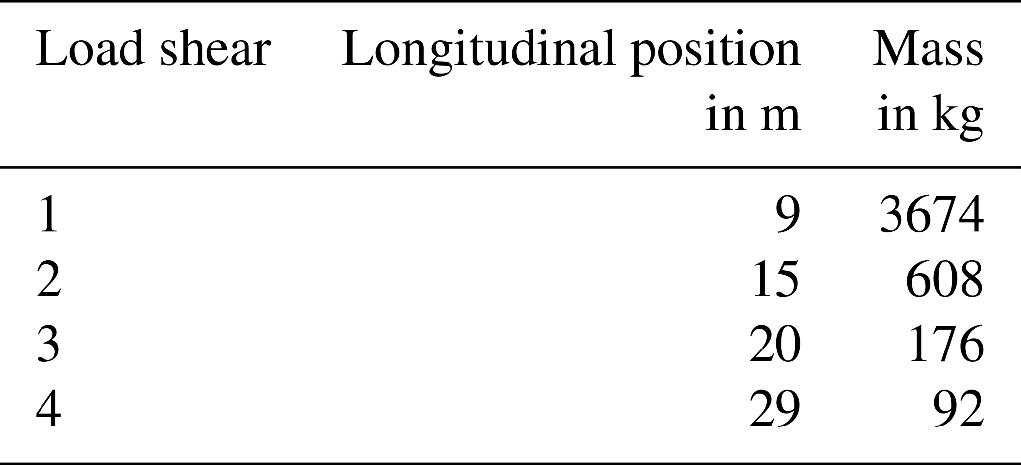
During the test, the blade was bolted to an adapter plate with the suction side facing downwards. Figure 1 shows the suspended laboratory rotor blade from different perspectives. Four load shears were mounted on the blade to apply the load and introduce a controllable bending moment. The longitudinal positions and masses of the four load shears are listed in Table 1.

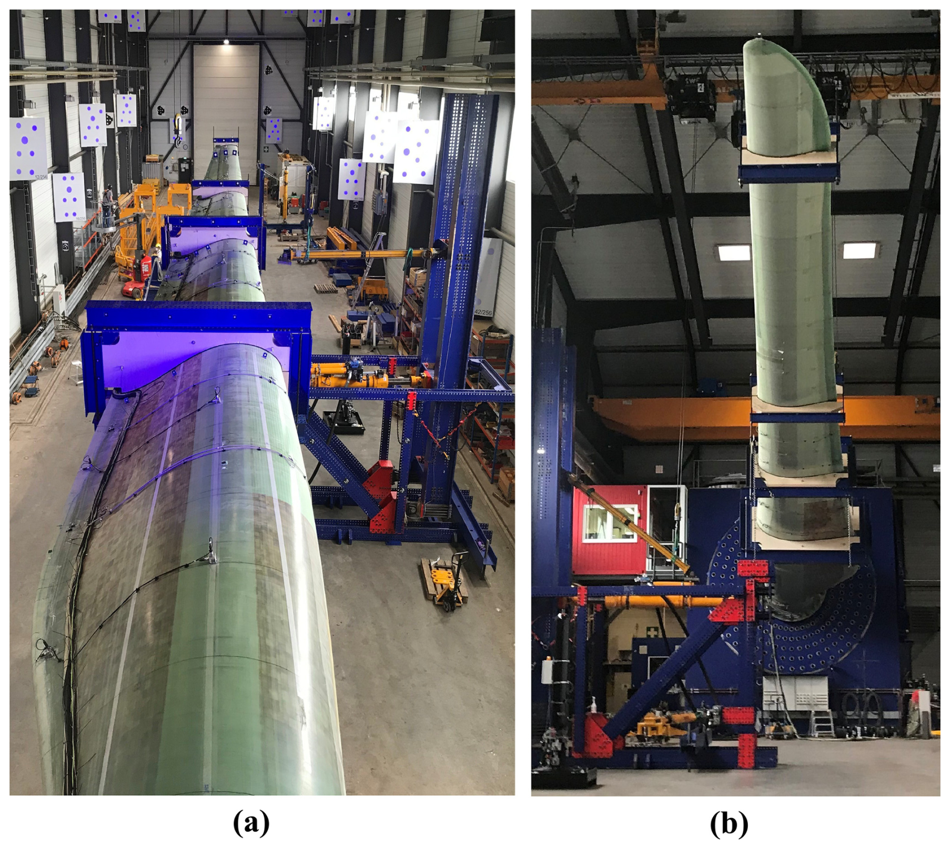
Figure 1 Suspended rotor blade in the test facility in Bremerhaven. (a) Pressure side. (b) Suction side.

Table 1 Load shear positions and masses.

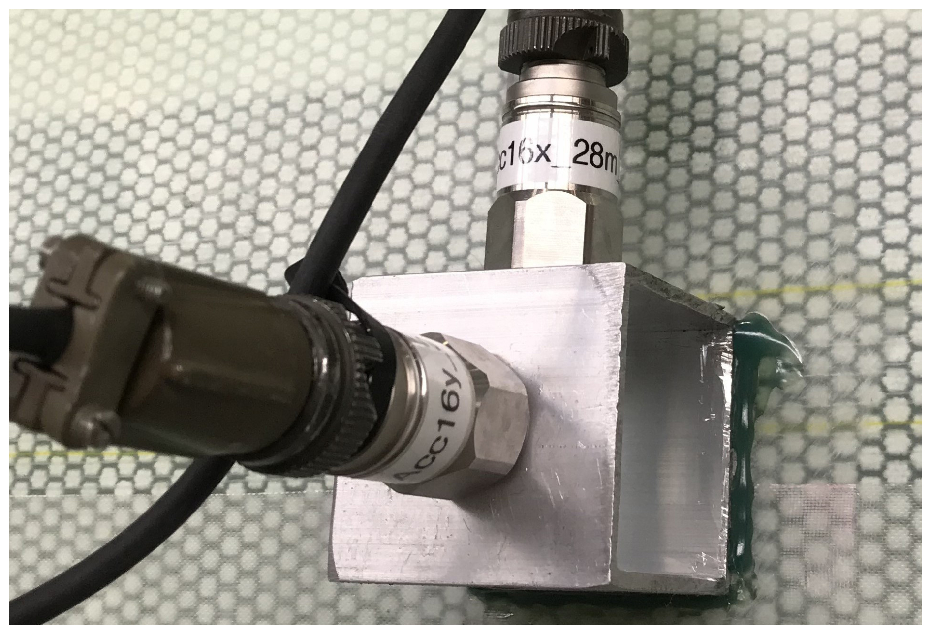
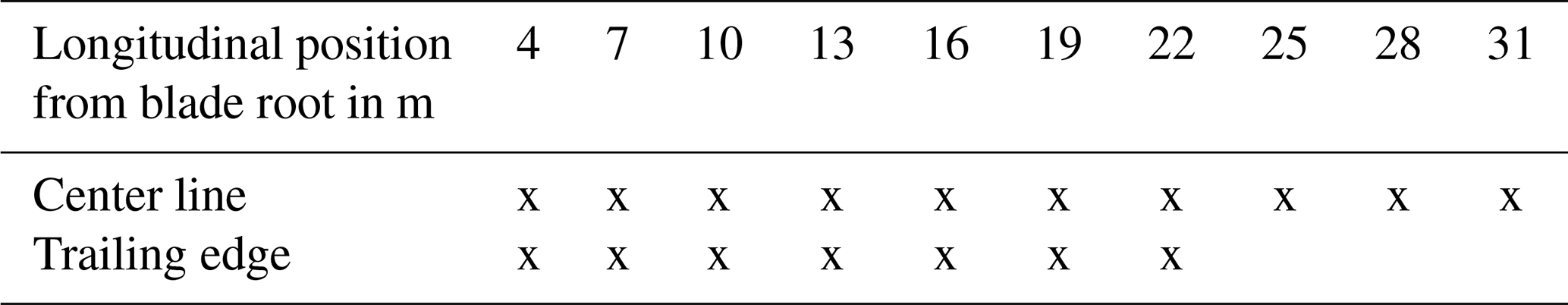
A total of 34 integrated electronics piezo-electric (IEPE) accelerometers with a dynamic range of ±100 m s⁻² were mounted on the pressure side (facing upwards) of the rotor blade. These accelerometers contain an internal charge amplifier, providing a voltage output proportional to acceleration, which enables high-sensitivity vibration measurements with low signal degradation over long cables. The sensors were placed every 3 m along the center line and the TE of the blade, as shown in Fig. 1a. Two accelerometers each were fixed at each sensor position at a 90° angle to each other in order to measure the flapwise and edgewise directions separately. Figure 2 shows an example sensor setup, and in Table 2, the longitudinal sensor positions are listed. As the cross-section of the rotor blade gradually tapers along the blade length, 10 sensor positions were located along the center line, and 7 sensor positions were located along the TE.

Figure 2 Example sensor setup with two accelerometers at a 90° angle.

Table 2 Sensor positions.

The fatigue load was introduced by a hydraulic cylinder connected to the second load shear at blade length L=15 m. The periodic excitation was carried out in edgewise direction close to the rotor blade's first eigenfrequency in this direction using a frequency of 1.59 Hz. The following fatigue load levels (FLLs) were set during the course of the rotor blade fatigue test:

• FLL 1 – ≈240 000 cycles with ±1700με (measured at L=12 m)

• FLL 2 – ≈425 000 cycles with ±1900με (measured at L=12 m)

• FLL 3 – ≈11 000 cycles with ±2000με (measured at L=6 m).

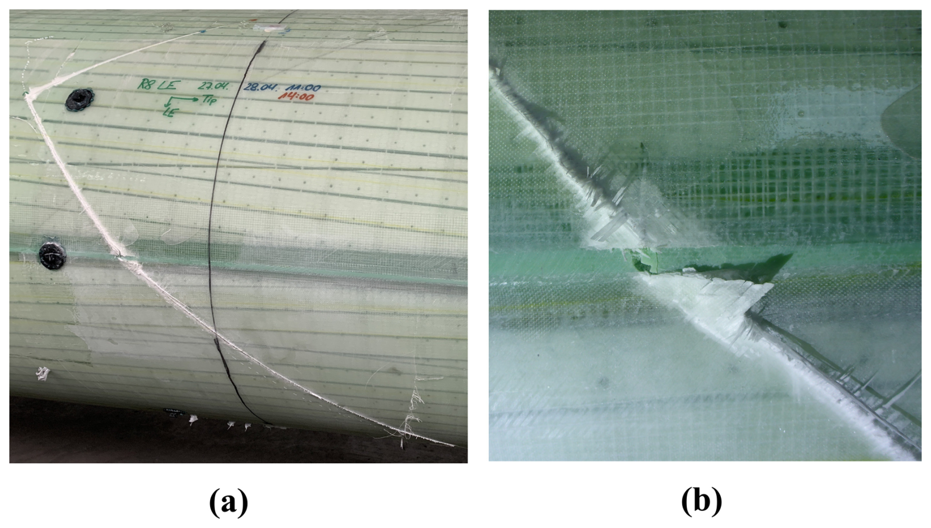
The amplitude of the hydraulic cylinder's motion was initially selected so that a material strain of ±1700με was measured at the TE of the blade at L=12 m using strain gauges. This load level was increased subsequently, and after approximately 11 000 cycles of the final FLL 3, the test was terminated due to the growth of a structurally critical crack at the LE, which most likely occurred due to fiber failure.

For the analysis of the different rotor blade states in between and after the application of the FLLs, dynamic tests were performed. These tests were carried out using dynamic shaker excitations, during which the rotor blade was decoupled from the hydraulic cylinder unit so that its motion was free of this constraint. The shaker was connected to load shear 2 at L=15 m. Each excitation was carried out in the edgewise direction using broadband white noise and lasted approximately 20 min. Table 3 provides an overview of the rotor blade states together with a description of the corresponding rotor blade's condition with respect to structural integrity. Figures 3 and 4 show photographs of the described fatigue cracks that occurred during the course of the test.

Table 3 Analysis states of the laboratory rotor blade to which shaker excitations were applied.

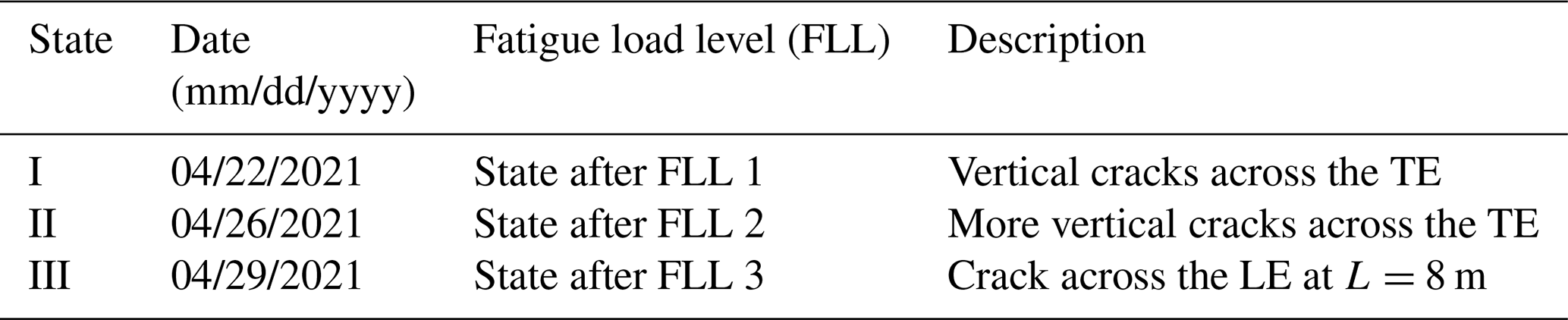
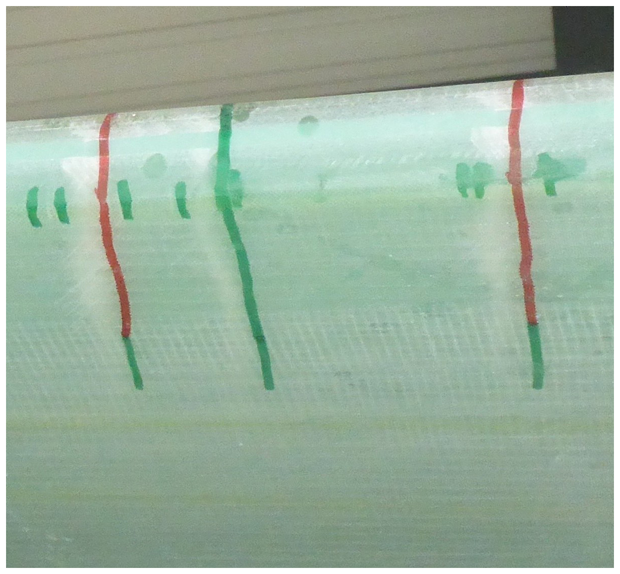
Figure 3 Vertical cracks across the TE traced out in red for state I and in green for state II.

Figure 4 Crack across the LE at L=8 m in state III. (a) Zoomed out. (b) Zoomed in.

3.1 Operational modal analysis

In this work, Bayesian operational modal analysis (BayOMA) (Au et al., 2013) is utilized for the identification of the modal parameters from the measurement data of the dynamic tests under broadband white noise excitation. The in-house implementation of the BayOMA was developed in MATLAB programming syntax and strictly follows the methodology described in detail in Au et al. (2013) and Au (2017). To ensure correctness and reproducibility of the implementation, the developed code has been thoroughly tested and compared with the established covariance-driven stochastic subspace identification (SSI-COV) (Jonscher et al., 2023).

During the measurements, the sampling rate was set to 100 Hz. Figure 5 illustrates the frequency spectrum including the first N_modes=5 eigenfrequencies of an example acceleration time period of the large-scale rotor blade recorded in state I. The frequency ranges f_area,i per eigenfrequency $i\in [\mathrm{1},N_{\mathrm{modes}}]$ utilized for the BayOMA are highlighted.

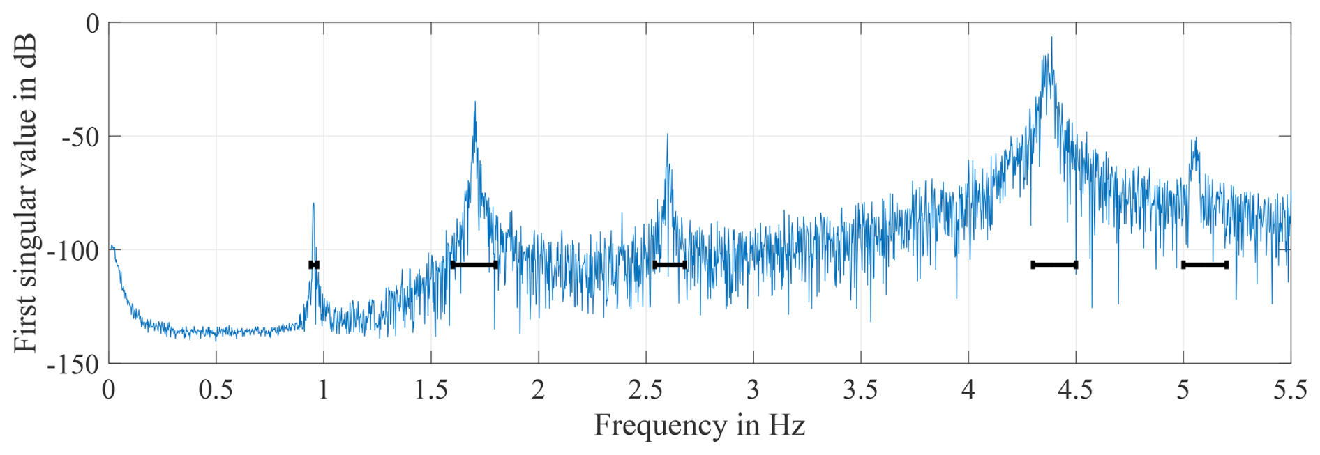
Figure 5 Frequency spectrum of the acceleration measurement in state I subject to broadband white noise excitation. The frequency ranges f_area,i per eigenfrequency $i\in [\mathrm{1},N_{\mathrm{modes}}]$ utilized for the BayOMA are highlighted.

To visualize the stability and consistency of the recorded measurement data over time, the measurement data were segmented into a number of datasets N_sets. The evaluation time period was set to T_data=400 s, and a moving window with an overlap of T_overlap=385 s was applied. For approximately 20 min=1200 s total measurement time, this results in N_sets=53 datasets. For each dataset, BayOMA was applied, resulting in 53 outputs which comprise the mean value and standard deviation of each eigenfrequency and the mean value and covariance matrix of each eigenmode. Figure 6 shows box plots of all eigenfrequency mean values ${\stackrel{\mathrm{‾}}{f}}_{\mathrm{M},i,j}$ identified from all 53 measurement datasets in the three different rotor blade states with $i\in [\mathrm{1},N_{\mathrm{modes}}]$ and $j\in [\mathrm{1},N_{\mathrm{sets}}]$.

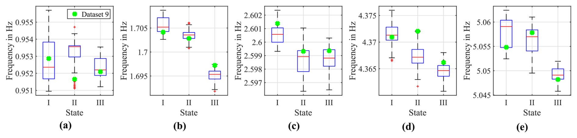
Figure 6 Box plots of the first five eigenfrequency mean values (a) ${\stackrel{\mathrm{‾}}{\mathit{f}}}_{\mathrm{M},\mathrm{1}}$ to (e) ${\stackrel{\mathrm{‾}}{\mathit{f}}}_{\mathrm{M},\mathrm{5}}$ of the rotor blade identified for each dataset in the three different analysis states using BayOMA. Box plot definitions: median (red line), interquartile range (blue box), extreme values (black whiskers), and outliers (red markers). Green crosses indicate the eigenfrequencies identified for dataset 9.

First of all, this analysis reveals that the interquartile ranges of the eigenfrequency mean values ${\stackrel{\mathrm{‾}}{\mathbf{f}}}_{\mathrm{M},i}$ remain stable for each observed rotor blade state. This indicates consistent measurements with no significant fluctuations or outliers due to the stationary laboratory conditions.

Looking more closely at the variation in the mean values of the five different eigenfrequencies across all states, it is clear that the eigenfrequencies ${\stackrel{\mathrm{‾}}{\mathbf{f}}}_{\mathrm{M},\mathrm{1}}$ and ${\stackrel{\mathrm{‾}}{\mathbf{f}}}_{\mathrm{M},\mathrm{3}}$, corresponding to flapwise bending mode shapes, are not significantly influenced by the damage that occurred during the fatigue test. In contrast, eigenfrequencies ${\stackrel{\mathrm{‾}}{\mathbf{f}}}_{\mathrm{M},\mathrm{2}}$, ${\stackrel{\mathrm{‾}}{\mathbf{f}}}_{\mathrm{M},\mathrm{4}}$, and ${\stackrel{\mathrm{‾}}{\mathbf{f}}}_{\mathrm{M},\mathrm{5}}$ exhibit a gradual reduction in magnitude, whereby the second and fourth eigenfrequencies correspond to edgewise bending mode shapes. The relative deviations of the first five eigenfrequencies between states I and III range from 0.02 % to 0.6 %.

The measured acceleration time series together with the BayOMA results of the three rotor blade states are published as open-access resources alongside this work within the public data repository of Leibniz University Hanover (Wolniak et al., 2025b).

3.2 Finite-element models

As both production and testing were carried out by Fraunhofer IWES, an outstanding feature of this rotor blade fatigue test was the complete documentation of the manufacturing process in addition to material and geometric data. Based on this detailed information, two different finite-element (FE) models were developed and employed for the model-updating procedures presented in this work. The simulations were performed using the FE analysis software Abaqus. Both numerical models are illustrated in Fig. 7, and summarized information regarding the element types, number of FEs, and the computing time for the modal analysis is given in Table 4. Here, the computing time comprises the setup of the model itself (i.e., the input file) and the modal analysis.

Figure 7 FE models of the 31 m wind turbine rotor blade. (a) Beam model. (b) Shell model.

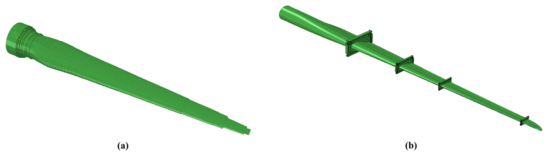
Table 4 Information regarding the two FE models utilized for the model updating of the laboratory rotor blade.

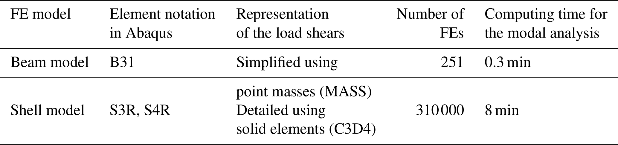
Firstly, a beam model was created based on the available cross-sectional characteristics of the rotor blade. Two-node linear beam elements, available in Abaqus as B31 elements, are selected, whereby a total of 251 beam elements are utilized. The B31 elements are based on the Timoshenko beam theory, allowing the representation of bending, axial, and torsional deformations along the beam axis. The varying sectional properties were assigned to the beam elements using general cross-sectional parameters. The load shears were simplified as point masses according to the information listed in Table 1 and assigned to the structure using concentrated mass elements in Abaqus. As the model-updating procedure applied in this work is based on the first five eigenfrequencies and corresponding eigenmodes, which are predominantly bending dominated, the rotational inertias of the load shears are not included. However, it should be noted that a more detailed representation of the load shears including the moments of inertia becomes increasingly relevant when torsional and higher-order modes are taken into account, which are not explicitly targeted in this work.

Secondly, a detailed shell model was set up based on the geometric data and composite layup available from the manufacturing process documentation. For this numerical model, S3R (three-node triangular) and S4R (four-node quadrilateral) shell elements with reduced integration were utilized. These elements efficiently capture bending, membrane, and transverse shear behavior, making them suitable for modeling thin to moderately thick shell structures. The load shears were modeled in detail using C3D4 tetrahedral solid elements and were included in all subsequent calculations, as they were attached during the whole experiment. In total, the shell model comprises approximately 310 000 FEs, of which around 81 700 are shell elements.

A comparison of the first five eigenfrequencies obtained from the beam model ($f_{\mathrm{S},\mathrm{Beam},i}$) and the shell model ($f_{\mathrm{S},\mathrm{Shell},i}$) is provided in Table 5. For an additional comparison between the numerical results and the modal parameters identified from the measurement data, the median eigenfrequencies ${\stackrel{\mathrm{̃}}{f}}_{\mathrm{M},\mathrm{I},i}$ computed from all mean eigenfrequencies in state I (cf. Fig. 6) are listed in Table 5. For a comparison of the corresponding eigenmodes, the modal assurance criterion (MAC) defined by Pastor et al. (2012),

$$\begin{array}{}\text{(17)}& \mathrm{MAC}({\mathit{\phi }}_{\mathrm{1}},{\mathit{\phi }}_{\mathrm{2}})={\displaystyle \frac{{\left|{\mathit{\phi }}_{\mathrm{1}}^{\mathrm{T}}{\mathit{\phi }}_{\mathrm{2}}\right|}^{\mathrm{2}}}{\left({\mathit{\phi }}_{\mathrm{1}}^{\mathrm{T}}{\mathit{\phi }}_{\mathrm{1}}\right)\left({\mathit{\phi }}_{\mathrm{2}}^{\mathrm{T}}{\mathit{\phi }}_{\mathrm{2}}\right)}},\end{array}$$

is evaluated between the respective eigenmodes and included in Table 5. The MAC quantifies the similarity between two (eigenmode) vectors, returning a value of 1 for linearly dependent vectors and 0 for linearly independent ones. In addition, a visual comparison of the eigenmodes of the beam and shell models and the eigenmodes identified from the measurement data is provided in Fig. 8. Again, the “measured” eigenmodes are represented using the median value computed from all mean eigenmodes identified in state I.

Table 5 Comparison of the first five modal parameters obtained from the beam and shell models and identified from the measurement data in state I.

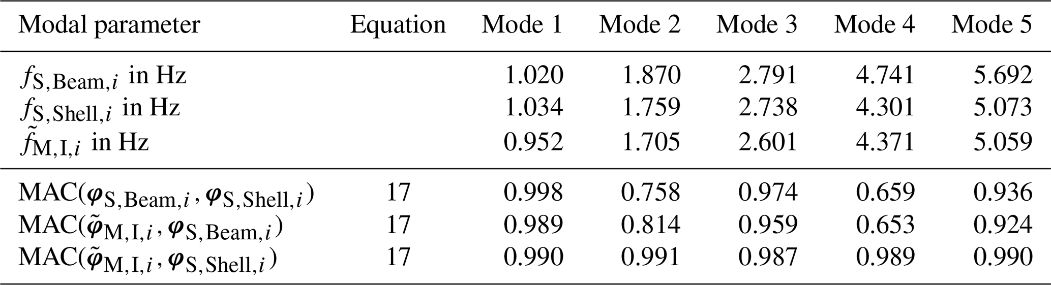
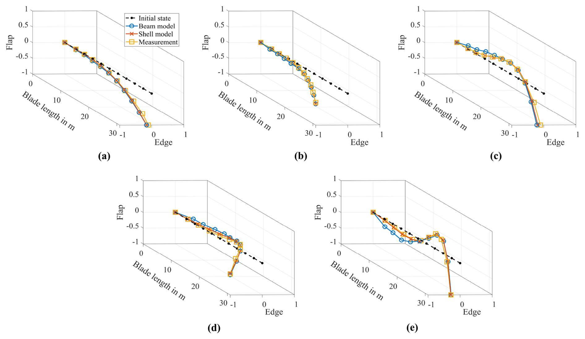
Figure 8 Comparison of the first five eigenmodes. Nos. (a) 1 to (e) 5 obtained from the beam and shell models and identified from the measurement data in state I.

4 Results

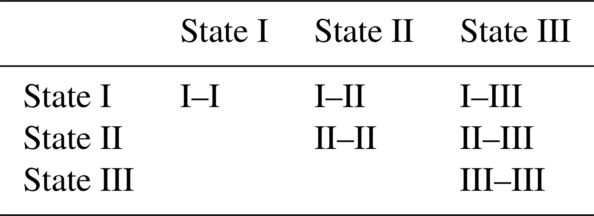
The following subsections present the results of the SDMU approach, applied using the three different design variable configurations (cf. Sect. 2.1.1, 2.1.2, and 2.1.3) with the objective of identifying damage in the considered laboratory rotor blade. For this purpose, all available rotor blade states listed in Table 3 are considered and systematically combined, yielding a total of six different state combinations. These combinations are summarized in Table 6, whereby the combinations along the diagonal represent self-comparisons of identical states.

Table 6 Rotor blade state combinations considered for the damage identification using the SDMU approach.

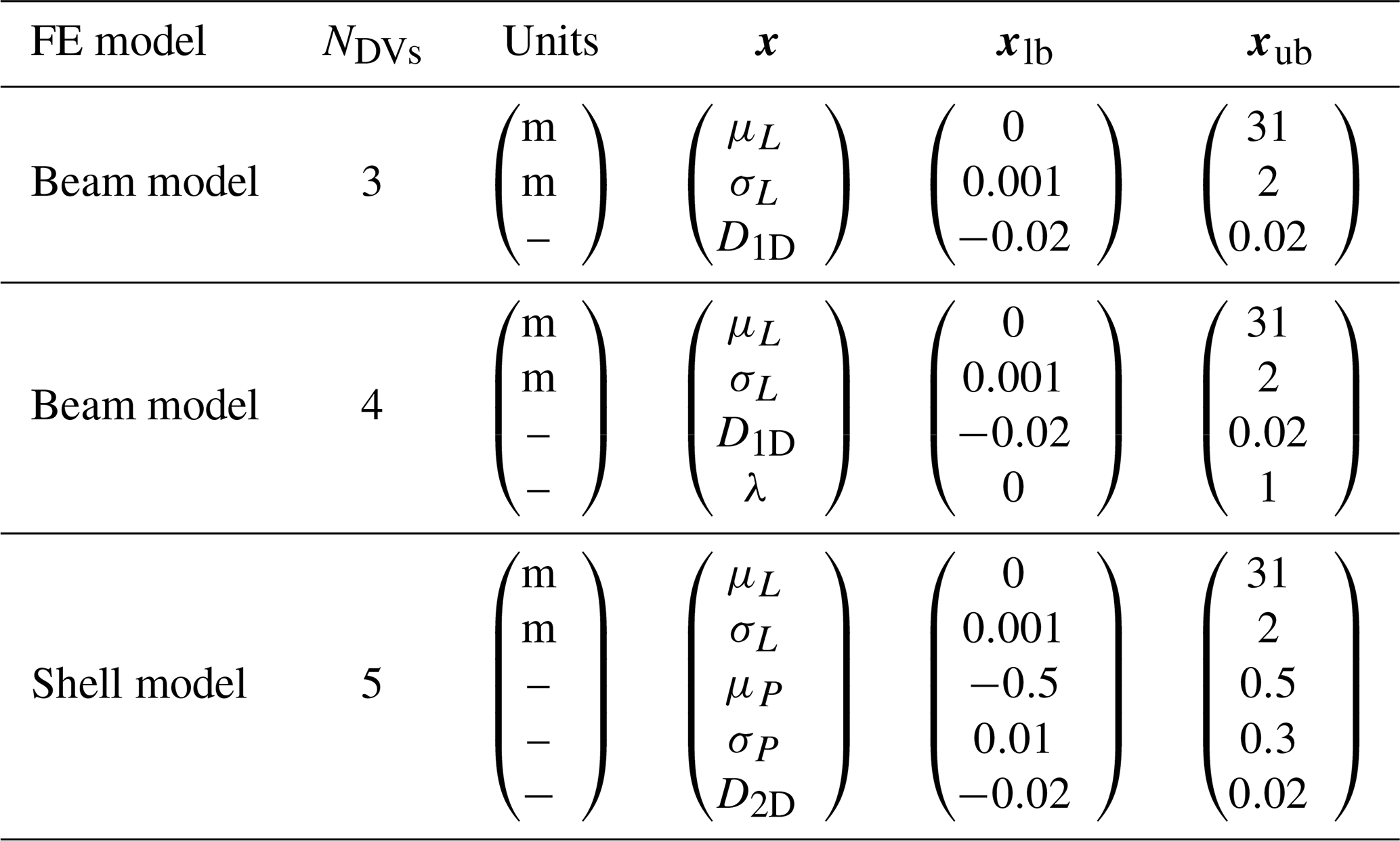
In this work, the SDMU approach is applied to three different design variable configurations, which feature different numbers of design variables N_DVs, each defining a damage distribution function. These configurations are associated with the two numerical models of different levels of detail. The upper and lower bounds x_ub and x_lb and physical units used for each design variable configuration are listed in Table 7, with the bounds of the three design variables, μ_L, σ_L, and D, shared by all three design variable configurations, chosen to be identical. Regarding the design variable σ_L, the lower bound was selected to ensure consistency with the smallest FE length in both FE models.

Table 7 Upper and lower bounds for the different design variable configurations.

To summarize and visualize the workflow, a schematic overview is provided in Fig. 9. The workflow begins with the data acquisition and subsequent data preparation, including the aforementioned segmentation of the recorded acceleration time series into N_sets datasets per rotor blade state. Following this, the BayOMA is performed for each dataset. Fast Fourier transform (FFT) is utilized to determine the initial values for the first tracked N_modes=5 eigenfrequencies $f_{\mathrm{M},i,j}$ and eigenmodes ${\mathit{\phi }}_{\mathrm{M},i,j}$ with $i\in [\mathrm{1},N_{\mathrm{modes}}]$ and $j\in [\mathrm{1},N_{\mathrm{sets}}]$. The first five eigenfrequencies and eigenmodes were selected because they could be reliably identified from the measurement data and reproduced with sufficient accuracy by both numerical models, which constitute fundamental prerequisites for a robust model-updating procedure. To ensure consistency and comparability across the performed model-updating procedures, the same set of modal parameters was employed for all rotor blade state combinations. Within the BayOMA, the optimization is conducted using a local optimization algorithm, more particularly, the MATLAB function fminsearch. The objective function is the negative log-likelihood function (NLLF), typically utilized in a Bayesian framework (Au, 2017). In addition, the frequency ranges f_area,i (cf. Fig. 5) are selected to be constant throughout all BayOMA applications.

Figure 9 Workflow from data acquisition to final results.

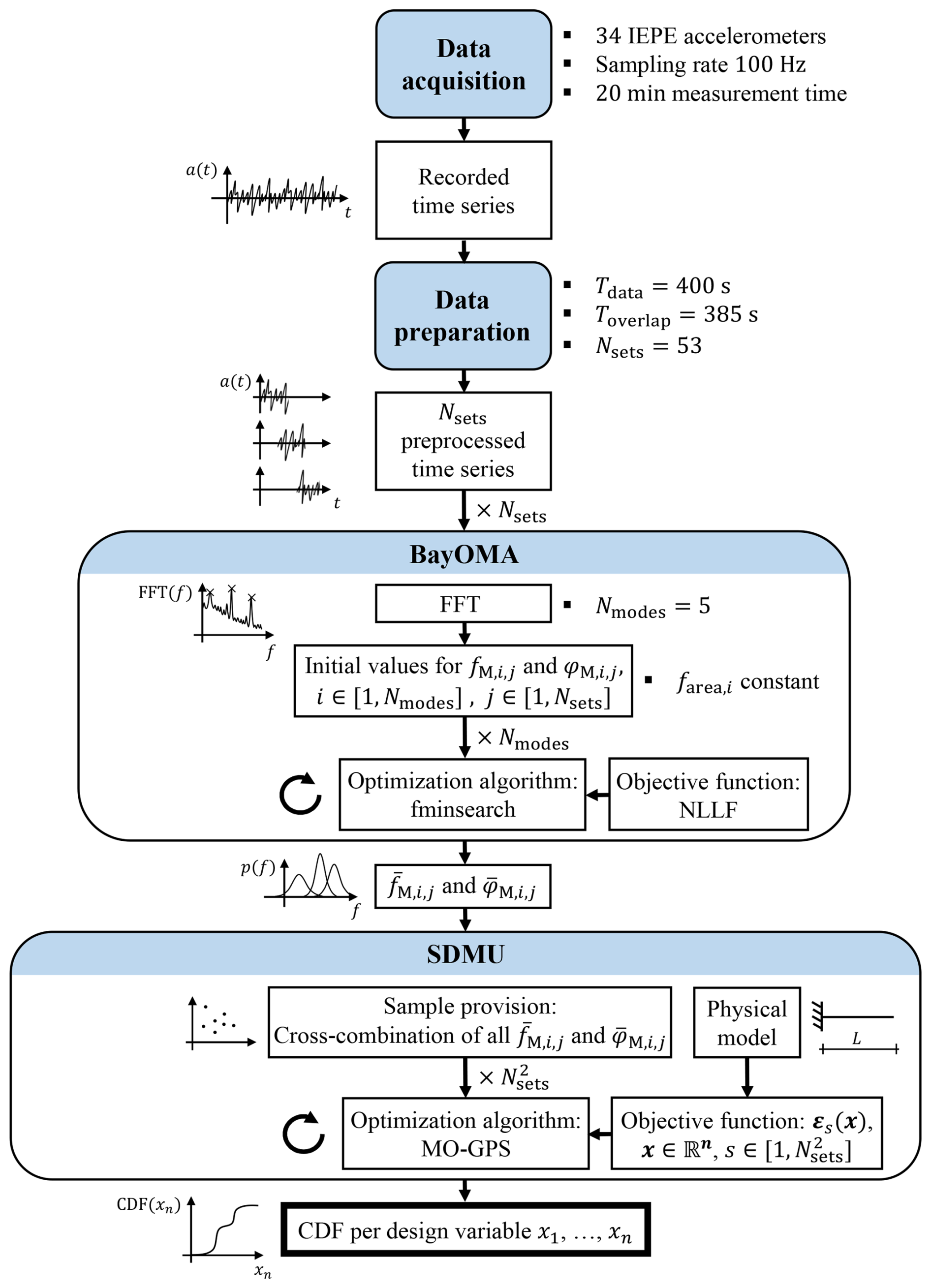
The outputs of all BayOMA applications are the most probable values (i.e., the mean values) of each eigenfrequency ${\stackrel{\mathrm{‾}}{f}}_{\mathrm{M},i,j}$ and eigenmode ${\stackrel{\mathrm{‾}}{\mathit{\phi }}}_{\mathrm{M},i,j}$ and represent the input for the subsequent SDMU procedure. For the sample provision within the SDMU procedure, these N_sets=53 modal parameter mean values identified for each reference and analysis (i.e., target) state are cross-combined using the Cartesian product. This results in a total of $N_{\mathrm{sets}}^{\mathrm{2}}=\mathrm{2809}$ input samples and, consequently, in the same number of $N_{\mathrm{sets}}^{\mathrm{2}}$ two-objective functions (cf. Eq. 13). The numerical optimization is carried out using the deterministic MO-GPS algorithm. Finally, cumulative distribution functions are calculated for each design variable based on all Pareto-efficient solutions obtained during an SDMU procedure (cf. Sect. 2.2).

The intent of using the cross-combination strategy, rather than an explicit sampling method, is to demonstrate that the SDMU approach can be applied independently of prior assumptions about the probability distribution of the input data. In this way, the method operates directly on discrete input realizations without requiring an explicit sampling procedure. Consequently, the generated sample set inherently reflects the frequentist uncertainty associated with the measurement and modal identification process. In this context, however, using cross-combination assumes that all modal parameters identified using BayOMA represent statistically independent and equally probable input samples for the numerical optimization. While this assumption allows for a straightforward and computationally efficient propagation of input uncertainty, it does not strictly correspond to sampling from a Bayesian posterior distribution and may lead to a conservative estimation of the resulting variance. As the measurement conditions were stationary, i.e., no significant variations in temperature, humidity, or other environmental factors occurred during the rotor blade fatigue test due to the laboratory environment, this assumption is considered reasonably well satisfied. Alternative strategies, such as Monte Carlo sampling from the BayOMA posterior or a sample provision based on the variance estimates provided by BayOMA, could provide a more rigorous probabilistic treatment of the input uncertainty. In particular, for applications involving significant environmental or operational variations, the present cross-combination strategy would no longer be sufficient, and an alternative sample provision approach would be required to account for the additional sources of input uncertainty.

4.1 Model-updating results using the beam model

To begin with, the damage identification results obtained using the beam model of the rotor blade are presented for the three- and four-dimensional design variable configurations, as introduced in Sect. 2.1.1 and 2.1.2, respectively. Before the application of the SDMU approach, preliminary studies are conducted to determine suitable settings for the input data and optimization algorithm hyperparameters. These studies are carried out using the three-dimensional design variable parameterization defined for the beam model with upper and lower bounds according to Table 7.

4.1.1 Settings

The first step of the SDMU approach is a single deterministic model-updating run using the numerical model – in this case, the beam model of the rotor blade. The resulting samples and corresponding modal parameters serve as the input data for the subsequent meta-model setup. Therefore, appropriate settings have to be defined for this initial deterministic model-updating run, forming the basis of the subsequent (meta)SDMU procedure.

Regarding the utilized MO-GPS optimization algorithm, two hyperparameters exist, namely the maximum number of objective function evaluations N_evals and the algorithm-specific number of tracked globally best coordinates T (Hofmeister et al., 2019). To evaluate which settings of N_evals and T are suitable, a convergence study is set up. To this end, a set of N_test=500 design variable samples is randomly generated in the design variable space (cf. Table 7), and the corresponding modal parameters are calculated using the beam model. These results are utilized as test data to evaluate each meta-model, set up using different combinations of N_evals and T. The evaluation of each combination is calculated using the root mean squared error (RMSE) of the first N_modes=5 eigenfrequencies, normalized by their respective value ranges:

$$\begin{array}{}\text{(18)}& \begin{array}{rl}{\mathit{\epsilon }}_{\mathrm{meta},f_i}& =\sqrt{{\displaystyle \frac{\mathrm{1}}{N_{\mathrm{test}}}}\sum _{s=\mathrm{1}}^{N_{\mathrm{test}}}{\left({\displaystyle \frac{f_{\mathrm{meta},\mathrm{S},i}\left({\mathit{x}}_{\mathrm{1}\mathrm{D},s}\right)-f_{\mathrm{S},i}\left({\mathit{x}}_{\mathrm{1}\mathrm{D},s}\right)}{f_{\mathrm{S},i,\max }\left({\mathit{x}}_{\mathrm{1}\mathrm{D}}\right)-f_{\mathrm{S},i,\min }\left({\mathit{x}}_{\mathrm{1}\mathrm{D}}\right)}}\right)}^{\mathrm{2}}}\\ & \mathrm{with}i\in [\mathrm{1},N_{\mathrm{modes}}],s\in [\mathrm{1},N_{\mathrm{test}}].\end{array}\end{array}$$

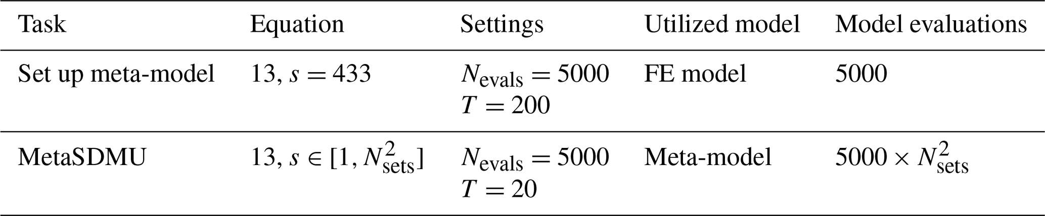
Figure 10 shows an example heat map for the relative eigenfrequency error ${\mathit{\epsilon }}_{\mathrm{meta},f_{\mathrm{1}}}$. The errors of the remaining eigenfrequencies are of similar magnitude. Notably, the meta-model error remains consistently low for T≥200 and N_evals≥2000. However, the minimum error is obtained for T=200 and N_evals=5000, which are therefore selected as the hyperparameter settings for the model-updating run used to populate the meta-model. Table 8 gives an overview of the different tasks performed during the SDMU procedure and the selected hyperparameter settings, in addition to a summary of the utilized model and the selected necessary model evaluations. A specific value for the computational time is not reported, as it strongly depends on several factors, such as the parallelization strategy, the employed hardware, the implementation of the optimization algorithm, and the model complexity. The computational time for a modal analysis using the different FE models is listed in Table 4.

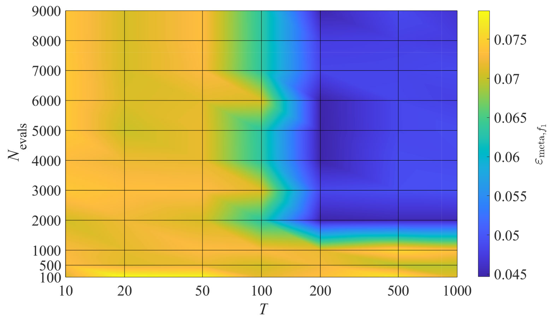
Figure 10 Evaluation of each meta-model set up using different combinations of N_evals and T. Surface colored according to the error ${\mathit{\epsilon }}_{\mathrm{meta},f_{\mathrm{1}}}$.

Table 8 Settings for the SDMU procedure.

For the initial deterministic model-updating run, only a single set of modal parameters can be used as input in the objective functions (cf. Eq. 13). As discussed in Sect. 3.1, the measurements show a high level of consistency without significant fluctuations or outliers. Consequently, the specific choice of the modal parameters used as input for the initial model-updating run is not critical. In this work, the modal parameters identified from the measurement data after a 2 min settling time are selected, corresponding to dataset number 9. The corresponding eigenfrequency mean values are marked in Fig. 6 with green crosses.

To verify that this set of modal parameters is indeed representative, model-updating runs with T=200 and N_evals=5000 are performed for all available datasets, shown as an example for combination I–III (cf. Table 6). In this context, a one-to-one mapping is employed. Figure 11 shows all N_sets=53 resulting CDFs for the three design variables. The results demonstrate that the choice of the input dataset has no significant effect on the model-updating results, confirming that the chosen dataset 9 (highlighted in green) is representative. Consequently, j=9 is selected for both rotor blade states to be compared, resulting in s=433 used in Eq. (13) for evaluating the two objective functions within the deterministic model-updating runs.

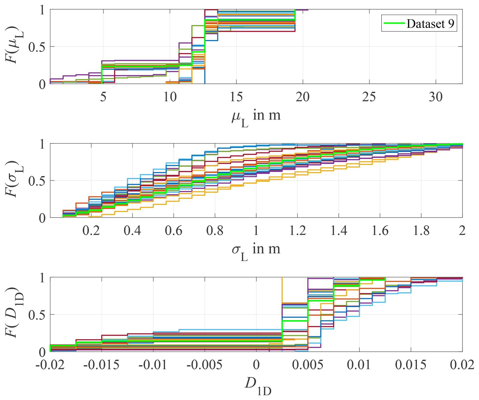
Figure 11 Resulting CDFs of the deterministic model-updating procedures for combination I–III based on the modal parameters of all datasets. The results for dataset 9 are highlighted in green.

4.1.2 Results for three design variables

This section presents the results obtained with the (meta)SDMU approach using the three-dimensional design variable configuration, which defines the one-dimensional damage distribution function applied to the beam model. For each state combination, the design variable samples and corresponding eigenfrequencies and eigenmodes from the initial deterministic model-updating runs serve as input for the meta-models, using the hyperparameter settings determined previously. Based on these meta-models and by applying Eq. (14), the metaSDMU procedure is carried out. As noted earlier, the N_sets=53 identified eigenfrequency and eigenmode mean values constitute the input samples and are cross-combined. This results in $N_{\mathrm{sets}}^{\mathrm{2}}=\mathrm{2809}$ two-objective functions, forming the basis of 2809 model-updating runs per combination, all of which are based on the corresponding meta-models.

Figure 12 shows the resulting CDFs for each design variable of each combination. The CDFs are derived from all optimal design variables obtained in the course of all $N_{\mathrm{sets}}^{\mathrm{2}}$ model-updating runs. For the combinations I–III and II–III, where state III represents the target state with the emerged crack at the TE of the rotor blade, the correct crack location and extent are highlighted in addition to the results for the design variables μ_L and σ_L. The crack extends longitudinally from ${\mathit{\mu }}_L=\mathrm{7.5}\mathrm{m}-\mathrm{8.5}$ m, yielding a correct damage width of 1 m. Using the basis of a Gaussian distribution function as spatial profile, μ_L and σ_L describe the geometric extent of the stiffness reduction (cf. Sect. 2.1.1). According to the definition of a Gaussian distribution function, the interval μ_L±1σ_L represents the region that contains approximately 68 % of the area under the spatial stiffness-reduction profile, whereas μ_L±2σ_L corresponds to roughly 95 %. Consequently, 2σ_L is associated with the correct damage extent of $\pm \mathrm{0.5}\mathrm{m}=\mathrm{1}$ m, resulting in a correct value for 1σ_L=0.25 m. Both values are highlighted in Fig. 12b. For the self-combinations I–I, II–II, and III–III, the known zero-damage intensity is highlighted in addition to the design variable D_1D. Moreover, the red crosses indicate a representative optimal design variable vector x_1D,optimal that is selected from the CDFs such that the first design variable, the damage position μ_L, is set to its median value ${\stackrel{\mathrm{̃}}{\mathit{\mu }}}_L$, defined as the 50 % value of the corresponding CDF.

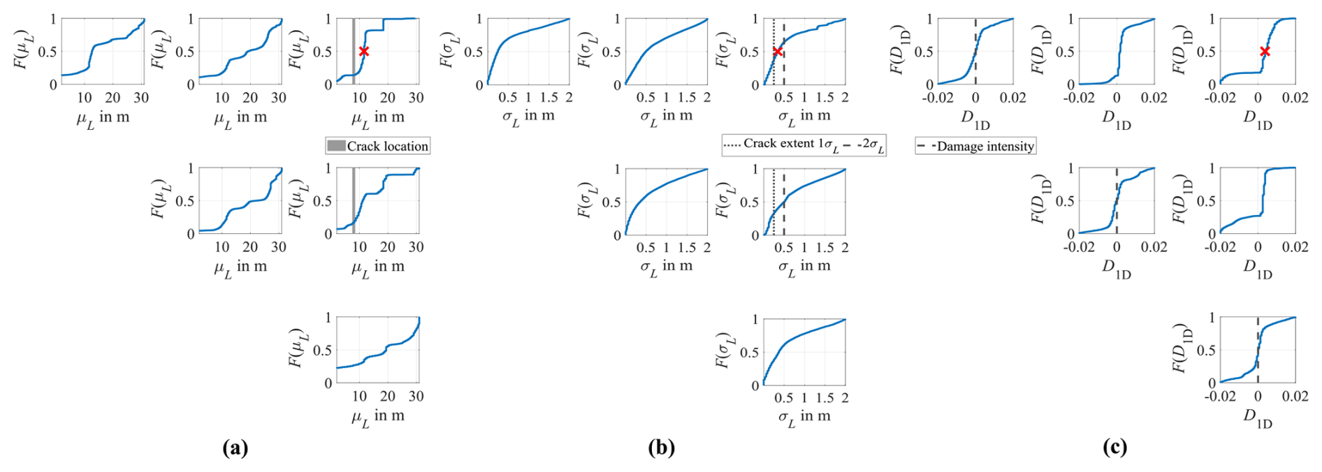
Figure 12 Resulting CDFs of the SDMU approach applied to the beam model using the one-dimensional damage distribution function parameterized by the three design variables (a) μ_L, (b) σ_L, and (c) D_1D, with settings given in Table 8. The red crosses added for combination I–III indicate an example optimal design variable vector.

Starting with combinations I–I, II–II, and III–III, where each state is compared with itself, the model-updating results are expected to reflect the absence of damage. The corresponding CDFs of the damage intensity D_1D, shown in Fig. 12c, are nearly identical, with D_1D=0 being the most probable outcome for all three self-comparisons. The results for design variable μ_L, shown in Fig. 12a, are also similar to each other, showing a sample distribution across the entire design variable space without clear probability clusters. Likewise, the longitudinal damage extent σ_L, shown in Fig. 12b, exhibits a similar pattern, with a slightly steeper slope for σ_L<0.5. Although the damage position and extent are not directly relevant when the damage intensity is zero, the lack of convergence in μ_L further confirms that no damage is present when these states are compared with themselves. In summary, with D_1D=0 as the most probable solution, the results for combinations I–I, II–II, and III–III consistently and correctly indicate that no damage is present in the rotor blade for these self-comparisons.

For combination I–II, comparing reference state I with analysis state II, no distinct damage position is apparent, as the design variable μ_L remains distributed across the design variable space. A similar pattern is observed for σ_L, again with a slightly steeper increase in the CDF for σ_L<0.5. However, the damage intensity D_1D shifts slightly from D_1D=0 to D_1D≈0.002 (cf. Fig. 12c). This indicates that damage has occurred, but no distinct position can be determined. This outcome is consistent with the target rotor blade state II, where numerous small vertical cracks appeared along the TE (cf. Fig. 3). Consequently, no single location is severely damaged; instead, the stiffness of the rotor blade is slightly reduced along the entire blade length due to these minor cracks.

Examining combinations I–III and II–III, where state III represents the target state with the most severe damage, the optimal damage intensity shifts to D_1D≈0.005. This positive value corresponds to a stiffness reduction in the rotor blade beam model according to the applied one-dimensional damage distribution function. In this context, it should be noted that the design variable D does not possess a direct physical interpretation in the same sense as the design variables μ_L and σ_L. Rather, it represents a phenomenological stiffness alteration within the numerical model, whereby a positive value corresponds to a stiffness reduction and a negative value corresponds to a stiffness increase. As the actual magnitude of damage is generally very difficult to quantify in fiber-reinforced composite material, an explicit validation of the identified value for D is not feasible for the considered rotor blade fatigue test. The location of the stiffness reduction is identified at μ_L≈ 11–12 m for both combinations, which deviates by approximately 3–4 m from the actual damage location at L=7.5–8.5 m. The results for the damage width σ_L, shown in Fig. 12b, are again spread across the design variable space. Compared to the solutions for all other combinations, the CDFs for combinations I–III and II–III show a noticeably steeper slope for σ_L<0.5 m, whereby the median value lies exactly between the 1σ_L and 2σ_L values highlighted in the figure. Consequently, this identified spatial damage extent corresponds reasonably well to the actual crack length of approximately 1 m.

To summarize, the SDMU procedure yields very similar results for combinations I–III and II–III, comparing states I and II to the same target state III. Moreover, for the self-combinations I–I, II–II, and III–III, the model-updating procedure consistently returns zero-damage results. These findings demonstrate the consistency and, consequently, the reliability of the applied SDMU approach, objective function formulation, and utilized design variable configuration.

To illustrate a representative damage distribution (i.e., stiffness reduction) for combination I–III, an example optimal design variable vector x_1D,optimal is selected from the CDFs such that the first design variable is set to its median value ${\stackrel{\mathrm{̃}}{\mathit{\mu }}}_L$. The remaining two design variables are chosen as the optimal values corresponding to this fixed first design variable, which, in the case of the beam model, also coincide with their respective median values. In Fig. 12, the example optimal design variable vector x_1D,optimal is indicated using red crosses. The stiffness reduction resulting from the one-dimensional damage distribution function based on x_1D,optimal is visualized in Fig. 13. For comparison, Fig. 14 visualizes the actual damage due to the crack that emerged at L≈8 m (cf. Fig. 4). It is evident that the found optimal crack location deviates from the correct location by approximately 3.5 m.

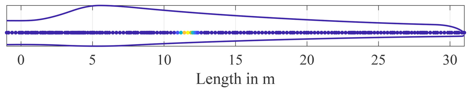
Figure 13 Visualization of the stiffness reduction based on x_1D,optimal, denoted by red crosses in Fig. 12, in the beam model. The schematic rotor blade geometry is additionally outlined.

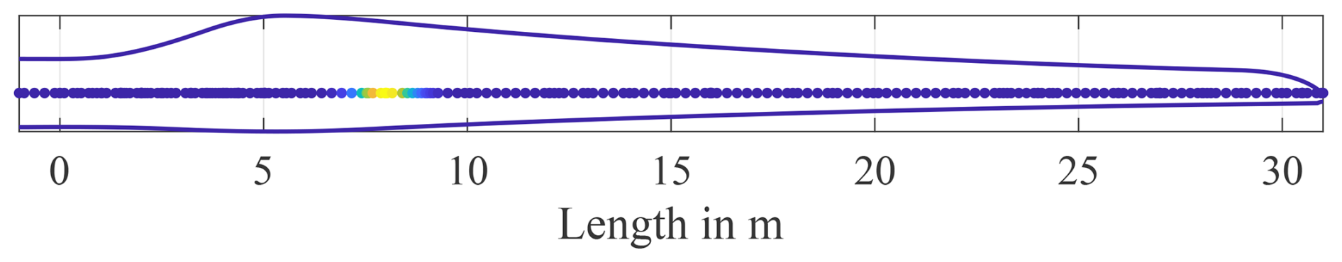
Figure 14 Visualization of the correct stiffness reduction in the beam model. The schematic rotor blade geometry is additionally outlined.

4.1.3 Results for four design variables

The results obtained using the four-dimensional parameterization of the one-dimensional damage distribution function, adding a separate consideration of the stiffness alterations in flapwise and edgewise directions via the design variable λ, are generally consistent with those presented above. Figure 15 shows the resulting CDFs of all optimal design variables for the six state combinations. As before, for combinations I–III and II–III, the correct damage location and spatial extent are highlighted in addition to the results for the design variables μ_L and σ_L. Moreover, the zero-damage results for all three self-comparisons are highlighted in addition to the results for the design variable D_1D.

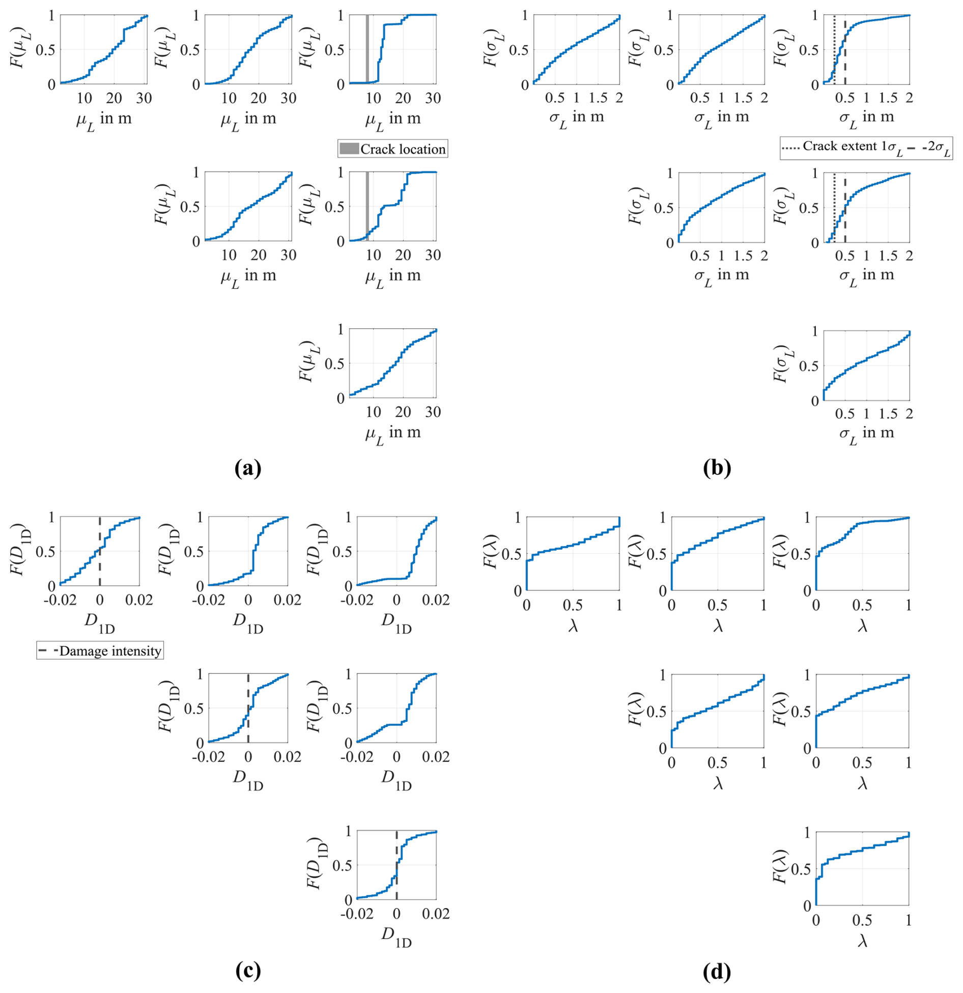
Figure 15 Resulting CDFs of the SDMU approach applied to the beam model using the one-dimensional damage distribution function parameterized by the four design variables (a) μ_L, (b) σ_L, (c) D_1D, and (d) λ, with settings given in Table 8.

Again, the design variable D_1D, shown in Fig. 15c, returns zero as the most probable outcome for all three self-comparisons and indicates a stiffness reduction for combinations I–II, I–III, and II–III. Closer examination reveals that the stiffness reduction increases from combination I–II to I–III and remains similar between combinations I–III and II–III. This is consistent with the observations from Fig. 12c. Similarly, the design variables μ_L and σ_L yield comparable results for the two design variable configurations applied to the beam model of the laboratory rotor blade.

Regarding the definition of the fourth design variable λ (cf. Sect. 2.1.2), a value of λ=0 implies a stiffness alteration applied in the edgewise direction, and a value of λ=1 implies a stiffness alteration applied in the flapwise direction. It is evident from Fig. 15d that λ=0 is the most probable solution for all combinations, indicating that mainly the stiffness in the edgewise direction is reduced, given that D_1D is positive. For combinations I–II, I–III, and II–III, this probability reaches approximately 50 %, while the self-comparisons show slightly less conclusive results.

Consequently, the separate consideration of the edgewise and flapwise directions captures the directional effect of the damage and provides an approximate indication of its positioning along the blade perimeter. However, the results should not be interpreted as ideal, since even in the self-comparison a significant probability of λ=0 is observed. Therefore, these findings should not be overemphasized. A true assessment of directional dependence would require the use of a shell model, which is presented in the following subsection.

4.2 Model updating using the shell model

Here, the damage identification results of the (meta)SDMU approach applied to the shell model of the laboratory rotor blade are presented. In this case, the two-dimensional damage distribution function parameterized by five design variables is utilized with upper and lower bounds according to Table 7.

In the initial deterministic model-updating run for each combination, the same settings as listed in Table 8 are employed. Based on the samples and corresponding eigenfrequencies and eigenmodes, the respective meta-models are created using the same settings as before.

Figure 16 shows the resulting CDFs obtained for each design variable of each combination. As before, these CDFs are calculated based on all optimal design variables identified in the course of all $N_{\mathrm{sets}}^{\mathrm{2}}$ separate model-updating runs for each input sample. For combinations I–III and II–III, the correct edgewise and flapwise locations of the emerged crack in state III are marked in gray. In addition, the 1σ and 2σ spatial damage extents are highlighted for both directions. For all three self-comparisons, the zero-damage result is highlighted. Furthermore, the red crosses indicate a possible optimal design variable vector x_2D,optimal for combination I–III.

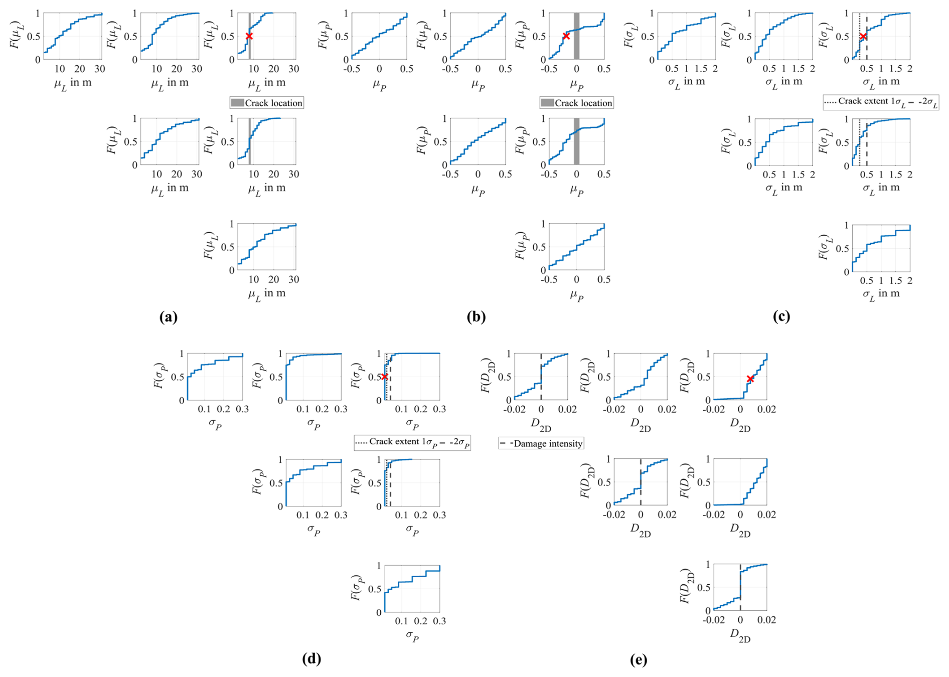
Figure 16 Resulting CDFs of the SDMU approach applied to the shell model using the two-dimensional damage distribution function parameterized by the five design variables (a) μ_L, (b) μ_P, (c) σ_L, (d) σ_P, and (e) D_2D. The red crosses added for combination I–III indicate an example optimal design variable vector.

For the design variable μ_L, shown in Fig. 16a, combinations I–III and II–III, with state III as the target state, clearly show that the damage localization along the blade length almost exactly matches the correct crack position. Most optimal values obtained using the shell model fall almost entirely in the gray-shaded area, representing the true damage location. In contrast, the results obtained using the beam model (cf. Figs. 12a and 15a) deviate from the damage position by approximately 3–4 m. This means that the shell model improves localization accuracy along the blade length. For combination II–III, the CDF also shows a short steep section at L=8 m. This indicates that the stiffness reduction has already begun at this location in state II, although it is less distinct than in state III. For combinations I–I, II–II, and III–III, no clear convergence of μ_L is observed, which is consistent with the expected zero-damage result for these self-comparisons.

Figure 16b displays the resulting CDFs for the damage position μ_P along the blade perimeter. For combinations I–I, I–II, II–II, and III–III, no clear convergence is visible, indicating that no specific position along the blade perimeter can be determined for these state combinations. For combinations I–III and II–III, a position between ${\mathit{\mu }}_P=-\mathrm{0.1}$ and ${\mathit{\mu }}_P=-\mathrm{0.3}$ is identified as the most probable solution. The negative sign corresponds to the pressure side of the blade, oriented upwards in the considered laboratory setup (cf. Fig. 1). This outcome does not match the true crack location across the LE in state III, corresponding to μ_P=0, as marked in gray. However, closer inspection of Fig. 4 shows that the crack propagates slightly more on the pressure side and changes direction through approximately 90° at this position. This may explain why the model-updating results identify the damage predominantly on the pressure side. Still, the damage localization along the blade perimeter remains complicated.

The results for the damage extent along the length σ_L, shown in Fig. 16c, are similar to those obtained using the beam model (cf. Figs. 12b and 15b), with the median lying exactly between the 1σ_L and 2σ_L values. The damage extent along the blade perimeter σ_P, shown in Fig. 16d, indicates a rather small spatial extent in this direction, with the median being even lower than the highlighted 1σ_P value. Consequently, the optimal results for the covariance matrix Σ_2D correspond to a crack-like shape extending in the longitudinal direction. While this reflects the characteristics of the real damage extent, the orientation does not correspond to the true extent across the LE of the rotor blade. However, it should be noted that an inclined damage extent, as is actually the case here (cf. Fig. 4), cannot be captured by the currently applied covariance matrix Σ_2D, since its off-diagonal terms are set to zero (cf. Sect. 2.1.3).

The results for the damage intensity D_2D, presented in Fig. 16e, follow a pattern across all combinations similar to that observed for the (meta)SDMU results using the beam model (cf. Figs. 12c and 15c). For the self-comparisons, D_2D=0 is the most probable outcome. Combination I–II shows an initial stiffness reduction, which is visible due to the slight rightward shift of the CDF. For combination I–III, the CDF shifts further to the right, revealing a more distinct solution for a positive D_2D. This indicates an even greater stiffness reduction. The results for combination II–III, also targeting state III, show a comparable solution for D_2D ranging from 0.025 to 0.175.

The stiffness reduction corresponding to the optimal design variable vector x_2D,optimal, marked in red in Fig. 16, is visualized in Fig. 17. Again, x_2D,optimal is selected such that the first design variable, the damage position μ_L, is set to its median value ${\stackrel{\mathrm{̃}}{\mathit{\mu }}}_L$, defined as the 50 % value of the corresponding CDF, while the remaining four design variables are chosen as the optimal values corresponding to this fixed first design variable. For the shell model, these corresponding values coincide with the respective median values regarding design variables σ_L, μ_P, and σ_P, whereas the corresponding optimal value for D_2D is slightly below its median. For comparison, Fig. 18 shows the correct damage location associated with the crack that emerged in state III. It should be noted that the “correct” representation aligns with the intuitive perception of the crack extending across the LE. This does not correspond to the actual crack propagation, which runs inclined across the LE (cf. Fig. 4). However, as mentioned before, this inclination cannot be captured by the applied five-dimensional design variable parameterization, as the off-diagonal terms of the covariance matrix Σ_2D are set to zero (cf. Sect. 2.1.3).

Figure 17 Visualization of the stiffness reduction based on x_2D,optimal, denoted by red crosses in Fig. 16, in the shell model. View of the (a) pressure side and (b) leading edge.

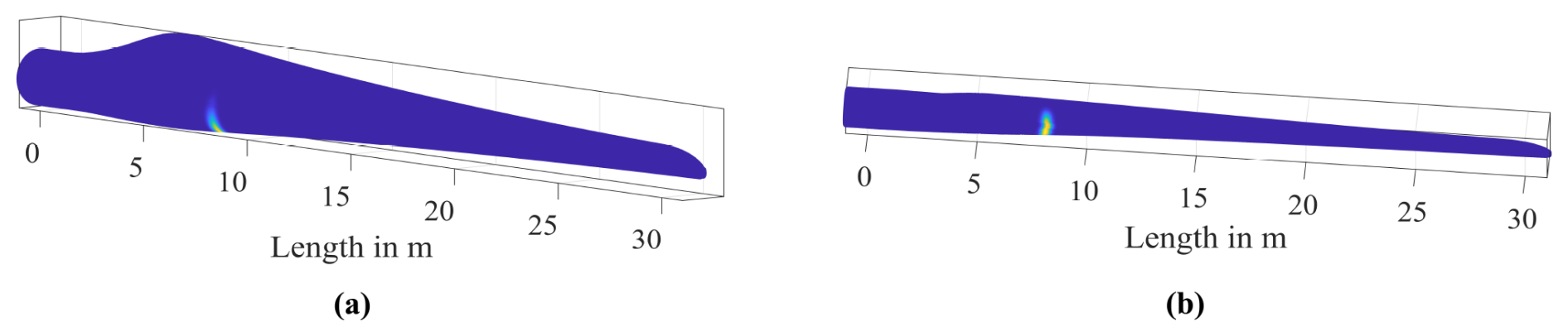
Figure 18 Visualization of the correct stiffness reduction in the shell model. View of the (a) pressure side and (b) leading edge.

In summary, the (meta)SDMU approach applied to the shell model of the rotor blade successfully localizes the damage along the blade length at L≈8 m. Furthermore, the damage exhibits an elongated, crack-like shape, which reflects the characteristics of the real damage extent. However, the found orientation is along the blade length rather than transverse to it, and the circumferential damage position was not accurately captured at the LE of the rotor blade but shifted towards its pressure side.

4.3 Comparison of the results

In this subsection, a direct comparison of the results obtained using the three different design variable configurations, defining the respective damage distribution functions applied to the two different numerical models, is presented. To illustrate this, Fig. 19 shows all the resulting CDFs for combination I–III. This combination updates the reference state I to the analysis state III of the laboratory rotor blade.

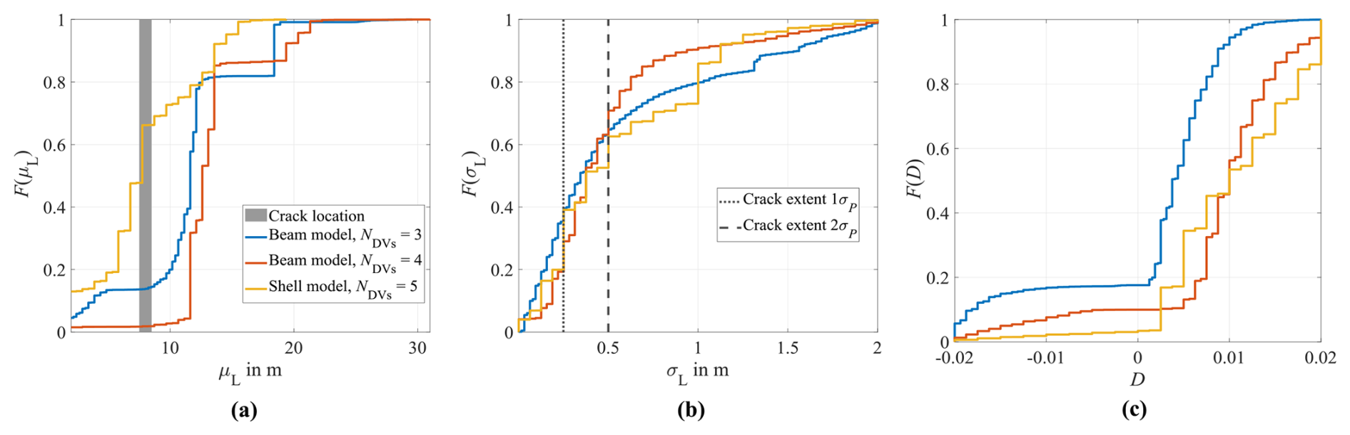
Figure 19 Resulting CDFs of the SDMU procedure for combination I–III – comparison of all three parameterizations of the damage distribution function. Design variables (a) μ_L, (b) σ_L, and (c) D.

In general, the results for the three design variables μ_L, σ_L, and D (i.e., D_1D and D_2D) show a high degree of similarity. This overall consistency confirms the methodological robustness of the presented (meta)SDMU approach and the validity of the three different implemented parameterizations of the damage distribution function. Moreover, the agreement across the results underlines their reliability, particularly given that two numerical models of distinctly different levels of accuracy and detail were employed.

However, upon closer inspection, some differences can be discerned. Most notably, the use of the more detailed shell model increases the accuracy of the damage localization along the blade length, shown in Fig. 19a. Table 9 summarizes the localization accuracy of the different design variable parameterizations using the beam and shell models with respect to the true damage position ${\widehat{\mathit{\mu }}}_L$ at L=8 m along the 31 m blade. Therefore, the medians ${\stackrel{\mathrm{̃}}{\mathit{\mu }}}_L$ – defined as the 50 % values of the CDFs – were calculated for each design variable configuration. To provide a quantitative metric for assessing the accuracy of the presented CDFs, Table 9 lists the relative error $e_{{\mathit{\mu }}_L}$ calculated in % per design variable configuration:

$$\begin{array}{}\text{(19)}& e_{{\mathit{\mu }}_L}=\mathrm{100}\times {\displaystyle \frac{{\widehat{\mathit{\mu }}}_L-{\stackrel{\mathrm{̃}}{\mathit{\mu }}}_L}{\mathrm{31}\mathrm{m}}}.\end{array}$$

Table 9 Comparison of the damage localization accuracy.

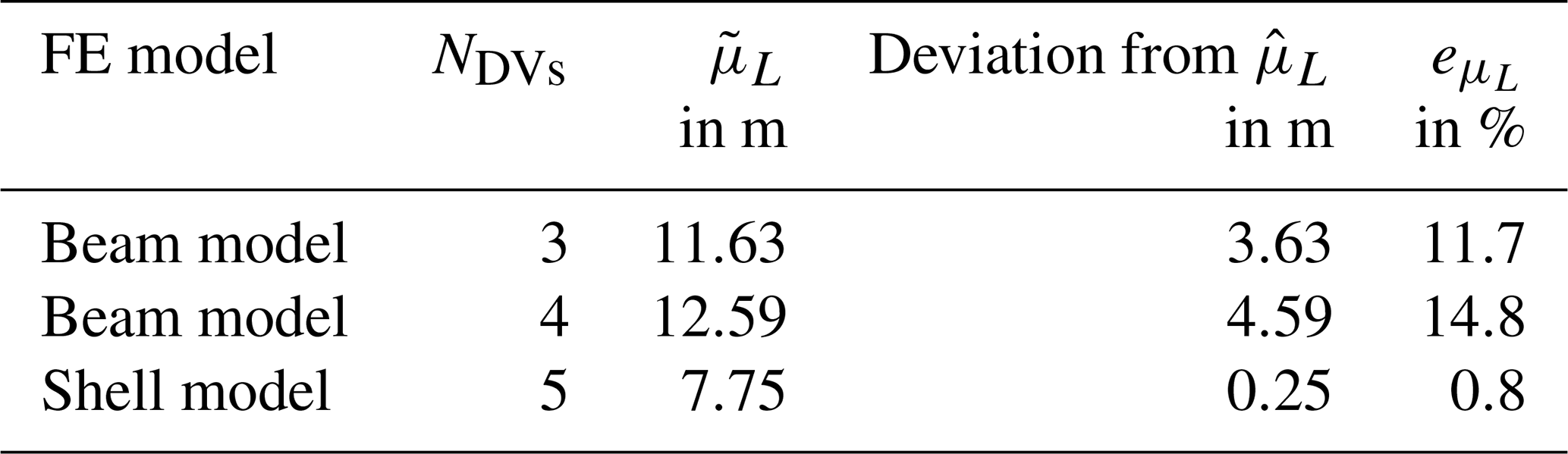
The listed results demonstrate that the shell model reduces the damage localization error to less than 1 % of the blade length. Due to its higher spatial resolution and more detailed representation of the blade geometry, it is significantly more accurate in capturing local damage. However, this accuracy comes with the need for detailed geometric and material information and the cost of higher computational demand, with a computing time of around 8 min, including the input file generation, model loading, and modal analysis. In contrast, the beam model provides a reasonably accurate damage localization within 11 %–15 % of the blade length despite its simplified representation, while requiring only around 20 s of computing time. This indicates that beam models can offer a practical compromise between computational efficiency and localization performance.

The damage extent is predicted nearly identically by all three parameterizations, illustrated in Fig. 19b. The true longitudinal extent of the inclined crack propagation is approximately 1 m, corresponding to a correct value of 2σ_L≈0.5 m and 1σ_L≈0.25 m, as respectively indicated by the vertical dashed and dotted lines in the figure. All in all, the three model-updating procedures accurately reflect the predominantly local nature of the damage.

Regarding the results obtained for the damage intensity shown in Fig. 19c, the beam model with three design variables predicts a slightly lower damage intensity, whereas the other two configurations yield similar results. Importantly, all three model-updating procedures consistently identify a stiffness reduction with high probability, indicating that the three presented damage parameterizations reliably capture the key structural effect of the damage. Again, it is noted that the value obtained for the design variable D cannot be explicitly validated for the considered rotor blade fatigue test, as the damage itself cannot be uniquely quantified. Although the crack, which finally occurred at the LE, can be visually identified, a quantification of the severity of this crack would require knowledge of geometric and mechanical characteristics such as the crack depth, crack tip opening displacement, and the specific damage mechanism. These parameters are typically not directly accessible and difficult to measure in a non-destructive manner. Moreover, the visible crack is likely not the only form of damage present in the blade, as it is very plausible that progressive material stiffness degradation occurred along the leading and trailing edges due to fatigue damage prior to the formation of the visible crack (cf. Fig. 3).

5 Conclusions

In this work, FE model updating was performed with the objective of damage identification based on a laboratory rotor blade fatigue test. Three rotor blade states were measured during the test, resulting in six possible state combinations to which the presented model-updating procedure was applied. The sample-based deterministic model-updating (SDMU) approach was employed, which, in this particular application, accounts for identification uncertainty in the modal parameters. Three different design variable configurations were introduced, each defining a damage distribution function used to update the stiffness of two numerical models with different levels of fidelity (beam and shell). This methodological framework enabled a systematic evaluation of how model detail and design variable parameterization influence the results of model updating.

In summary, all three design variable configurations yielded consistent results across all six state combinations, confirming the robustness of the SDMU approach and validating the implemented parameterizations of the damage distribution function. The agreement among the results underlines their reliability, particularly given that two numerical models of distinctly different levels of accuracy and detail were employed. As expected, all model-updating procedures returned zero-damage results for the three self-comparisons and revealed a progressively increasing stiffness reduction together with a conclusive damage localization along the blade length. The most notable difference between the two utilized FE models was revealed with respect to the longitudinal damage localization. While the use of the shell model allows for a damage localization within less than 1 % of the blade length, the use of the beam model achieved an accuracy of only 11 %, deviating from the true damage position by 3.5 m.

The findings of this work underline the importance of defining the analysis objective in advance. Naturally, the choice of the numerical model depends on whether computational efficiency or model accuracy is the primary goal. When a fast overview of the general damage vicinity is required, the beam model provides a computationally efficient solution. In contrast, the shell model is more appropriate when precise damage localization is needed, including the localization along the perimeter. The application of a model selection approach is also possible to support the choice based on a quantitative metric. However, this becomes increasingly relevant when a larger set of competing models is available.

As the considered five-dimensional design variable parameterization applied to the shell model does not account for inclined damage extents, incorporating the off-diagonal terms of the covariance matrix represents an interesting extension. In addition, a sensitivity study with regard to the choice of the distribution function representing the damaged area would provide valuable insight for assessing the robustness of the proposed model-updating approach. Future work should also aim to include model uncertainty in the SDMU approach. Furthermore, a comparison between the presented results using the cross-combination strategy, assuming statistically independent and equally probable input samples, and results obtained using an alternative sampling method represents an interesting outlook. Moreover, the present study is limited to a laboratory experiment without realistic variation of environmental or operational conditions, which are of high relevance for rotor blades. Addressing these aspects will provide valuable extensions and enhancements to the presented model-updating approach.