Modelling vortex generator effects on turbulent boundary layers with integral boundary layer equations

Vortex generators (VGs) are known to delay separation and stall, allowing the design of airfoils with larger stall margins, particularly for thick airfoil sections in the inboard and midboard regions of modern slender wind turbine blades. Including VG effects in blade design studies requires accurate VG models for fast lower-order techniques, like integral boundary layer (IBL) methods. Previous VG models for IBL methods have used engineering approaches tuned on airfoil aerodynamic data. The accuracy of these models depends on the availability of wind tunnel aerodynamic polar datasets for tuning, which are limited and time-consuming to expand for the relevant wind conditions, airfoil sections, and VG configurations being used in continuously growing wind turbine blades. This work proposes a VG model using IBL equations derived from flat-plate boundary layers under the influence of VGs. The new VG model empirically models the shape factor of the boundary layer and the viscous dissipation coefficient in the IBL framework to account for the additional momentum and dissipation in the boundary layer mean flow due to VGs. The model is developed from a wide range of flat-plate boundary layers and VGs to account for variations in VG vane size and placement on the turbulent boundary layer development influencing the airfoil aerodynamic characteristics. The new VG model, called RFOILVogue, is implemented in an in-house code RFOIL, an improvement over XFOIL, and validated with computational fluid dynamics (CFD) data and wind tunnel measurements of flat plates and airfoil sections equipped with VGs. Since it is derived from vortex dynamics in turbulent boundary layers, RFOILVogue better predicts both airfoil performance characteristics, such as positive stall angle, maximum lift, and drag, and boundary layer flow parameters, such as the separation location, compared to the existing tuned VG models. The VG model still suffers from some inherent drawbacks of reduced-order models like RFOIL, and future research directions for thick airfoils are proposed to overcome these drawbacks in VG modelling.

1 Introduction

Studies on the projected capacity of future wind turbine rotors indicate an increasing trend for larger rotors with lower induction and blades far beyond 100 m in radius (Jensen et al., 2017; Schepers et al., 2015). Relatively thicker airfoils must be employed along the entire blade span to balance the aero-structural loads, ensure structural integrity, and reduce deformations. These thicker airfoils are more prone to flow separation, with the consequent loss in lift leading to a decrease in annual energy production (AEP) and an increase in fatigue loading, affecting the structural health of the blades (McKenna et al., 2016). Vortex generators (VGs) are conventionally adopted as passive flow control devices, primarily delaying flow separation at moderate angles of attack and consequently improving the maximum lift of these thicker airfoil sections (Lin, 2002; Baldacchino et al., 2018). With turbines growing in size, it is common to see their installation up to the most outboard blade sections to ensure optimal aerodynamic performance in a broader range of operating conditions (Bak et al., 2016). Their application has additionally been shown to mitigate the effects of leading-edge erosion, partially restoring the original airfoil design conditions (Gutiérrez et al., 2020; Ravishankara et al., 2020). The performance prediction of VGs becomes very important in the design phase to avoid unacceptable changes in loading, especially considering their installation on progressively outboard sections on the blade.

While wind tunnel campaigns and numerical modelling with computational fluid dynamics (CFD) are sufficient to analyse the effect of VGs on 3D boundary layers and flow separation characteristics as add-ons, high-fidelity computations can actually prove prohibitive in including VGs in blade design optimisation routines due to computational costs (Aparicio et al., 2015; Gonzalez et al., 2016; Gonzalez-Salcedo et al., 2020). Despite the development of partly modelled and partly resolved approaches like the Bender–Anderson–Yagle (BAY) model (Bender et al., 1999; Jirásek, 2005; Manolesos et al., 2020) to aid faster CFD analysis of VGs, as well as recent advances in computational capacity, these methods still require a significant computational time of the order of several weeks. Blade design optimisation routines usually employ reduced-order, computationally efficient tools like XFOIL (Drela, 1989) and RFOIL (Van Rooij, 1996) developed using flow field data from higher-order methods like CFD or flow measurements. XFOIL and RFOIL couple an inviscid panel method to a viscous boundary layer solver based on the integral boundary layer (IBL) equations. Both tools excel in predicting the lift and drag characteristics of airfoils in natural and forced transition at low and medium angles of attack just after stall, with limited capabilities for deep stall (Drela, 1989; Van Rooij, 1996).

Previous studies in the literature have proposed modelling the effect of the streamwise vortices caused by VGs as an additional source of turbulence in the boundary layer to predict the performance of VGs with IBL equations correctly. Kerho and Kramer (2003) proposed modifying the equation of turbulent shear stress lag (Green et al., 1977) in the system of IBL equations by including the added turbulence as a source term. Modification of the turbulent shear stress lag equation was also the fundamental basis of the engineering models developed by De Tavernier et al. (2018) and Daniele et al. (2019). All three previous models employed a source term that appears at the VG location and dissipates downstream of the VG location to incorporate the effect of VGs as extra turbulence production in the boundary layer. All three models used tunable coefficients in the source term formulation for representative test cases. The implementation of De Tavernier et al. (2018) adopted a multivariate regression of several coefficients based on the lift polars of a larger database of airfoils and VG parameters, leading to a more widely usable implementation in XFOIL called XFOILVG. XFOILVG's implementation has also been coupled to a double-wake panel method for dynamic stall calculations of airfoils equipped with VGs (Yu et al., 2024).

In the past work of Sahoo et al. (2024), the authors validated the added turbulent source term model and its assumptions. The VG model from De Tavernier et al. (2018) was implemented in RFOIL, an improvement over XFOIL, and the lift behaviour predictions of both RFOILVG and XFOILVG were benchmarked against an extensive database of aerodynamic data of airfoil sections with different VG geometries. The benchmark showed that XFOILVG and RFOILVG overpredicted the maximum positive lift and stall angle for airfoils and VGs outside the training dataset. This was also seen in the work of Yu et al. (2024). The benchmark concluded that the only way of improving such an engineering model is by training it on broader datasets representative of the changing VG types, airfoils, and Reynolds numbers for modern wind turbines. The lack of wind tunnel data for relatively thicker airfoils with VGs thus limits the improvement of this tuned engineering model.

The literature also shows that the underlying assumption behind previous models – modelling VGs as additional turbulence production in the boundary layer – is incomplete. Numerical and experimental studies on vortices in turbulent boundary layers show that both turbulent fluctuations and mean velocity profiles are modified (Squire, 1965; Von Stillfried et al., 2009; von Stillfried et al., 2011; Velte et al., 2014; Baldacchino et al., 2015; Gutierrez-Amo et al., 2018). The mean flow transport due to the vortices causes a redistribution of momentum and energy, leading to changes in all three components of velocities and spatial gradients. In particular, the spanwise velocities, stresses, and gradients can no longer be neglected when formulating the IBL equations from the Navier–Stokes equations. These studies show that statistical models that model the effect of VGs as turbulent forcing underpredict the shear stress and the pressure gradient evolution. Even though changes in the integral boundary layer quantities have been reported independently in the literature by Schubauer and Spangenberg (1960), Gould (1956), and Lögdberg et al. (2009), existing models do not relate these changes to changes in the mean flow. This work fills this gap with a VG model in the IBL framework that incorporates the changes in the mean flow due to VGs to predict the boundary layer characteristics.

1.1 Present research

In this work, we first present the new IBL equations for VGs, derived from the mean flow changes, containing additional terms to account for the missing factors. We then present a methodology to model the most significant new and modified terms, relating VG array geometry parameters and the flow Reynolds numbers to the modelled IBL quantities. Thus, unlike the previously proposed tuned models that did not account for any vortex dynamics, the proposed VG model relates the changes in IBL quantities to the dynamics of streamwise vortices embedded inside the turbulent boundary layer. This results in an analytical model independent of airfoil tuning data that captures the evolution of IBL quantities in the span and downstream of VGs. The proposed VG model is valid for counter-rotating VG arrays, which are the type of array most commonly used in wind turbines, and has been shown to be the most effective VG arrangement for flow separation control in previous studies in the literature (Gould, 1956; Baldacchino et al., 2018).

The paper is organised as follows. Section 2 gives the background on the original IBL equations used in XFOIL/RFOIL. Section 3 details the setup of the CFD simulations used to generate the flat-plate boundary layer data with and without VGs used to develop the proposed model. Section 4 describes the new equations due to VGs, the most significant IBL terms, and the model used to integrate these changes in RFOIL. The implementation in RFOIL is first verified against CFD data in Sect. 6 by recreating an approximate flat plate in RFOIL. Subsequently, the new model's performance is benchmarked against reference wind tunnel data (summarised in Appendix A) and compared to the old models. Section 7 discusses the model performance for some selected test cases, and Sect. 8 summarises the performance assessment for the complete reference database. Section 9 concludes the paper by summarising the main improvements, limitations, and an outlook on future work to improve the new model further.

2 Integral boundary layer equations

XFOIL and RFOIL are viscous–inviscid interaction tools that split the flow around airfoils into an inviscid outer flow solved with a linear vorticity stream function panel method coupled to an inner viscous boundary layer flow solved with the IBL method (Drela, 1989). RFOIL improves XFOIL's IBL formulation for airfoil sections near stall experiencing 3D rotational flow on wind turbine blades through additional rotational corrections, thick airfoil drag corrections, and numerical stability corrections (Snel et al., 1993, 1994; Van Rooij, 1996; Ramanujam et al., 2016). For the sake of simplicity, we discuss the VG model using the original XFOIL equations without RFOIL's additional improvement terms. As such, the VG model can be applied to the IBL framework independent of RFOIL's other improvements. The original IBL equations are presented in Eqs. (1)–(3). Details of their derivation from the Navier–Stokes equations can be found in the literature, such as Whitfield (1978), White (2006), and Özdemir (2020).

$$\begin{array}{}\text{(1)}& {\displaystyle \frac{\mathrm{d}\mathit{\theta }}{\mathrm{d}x}}={\displaystyle \frac{C_{\mathrm{f}}}{\mathrm{2}}}-\left(H+\mathrm{2}\right){\displaystyle \frac{\mathit{\theta }}{U_{\mathrm{e}}}}{\displaystyle \frac{\mathrm{d}{U}_{\mathrm{e}}}{\mathrm{d}x}}\text{(2)}& {\displaystyle \frac{\mathrm{d}{H}^{*}}{\mathrm{d}x}}={\displaystyle \frac{\mathrm{2}{C}_{\mathcal{D}}}{\mathit{\theta }}}-{\displaystyle \frac{H^{*}}{\mathit{\theta }}}{\displaystyle \frac{C_{\mathrm{f}}}{\mathrm{2}}}-\left(\mathrm{1}-H\right){\displaystyle \frac{H^{*}}{U_{\mathrm{e}}}}{\displaystyle \frac{\mathrm{d}{U}_{\mathrm{e}}}{\mathrm{d}x}}\text{(3)}& {\displaystyle }\begin{array}{rl}{\displaystyle \frac{\mathit{\delta }}{C_{\mathit{\tau }}}}{\displaystyle \frac{\mathrm{d}{C}_{\mathit{\tau }}}{\mathrm{d}x}}& =K_c\left({C_{{\mathit{\tau }}_{\mathrm{EQ}}}}^{\frac{\mathrm{1}}{\mathrm{2}}}-{C_{\mathit{\tau }}}^{\frac{\mathrm{1}}{\mathrm{2}}}\right)\\ & +\mathrm{2}\mathit{\delta }\left({\displaystyle \frac{\mathrm{4}}{B{\mathit{\delta }}^{\ast }}}\left({\displaystyle \frac{C_{\mathrm{f}}}{\mathrm{2}}}-{\left({\displaystyle \frac{H-\mathrm{1}}{AH}}\right)}^{\mathrm{2}}\right)-{\displaystyle \frac{\mathrm{1}}{U_{\mathrm{e}}}}{\displaystyle \frac{\mathrm{d}{U}_{\mathrm{e}}}{\mathrm{d}x}}\right)\end{array}\end{array}$$

Here δ is the boundary layer thickness, δ^∗ is the displacement thickness, θ is the momentum thickness, $H=\frac{{\mathit{\delta }}^{\ast }}{\mathit{\theta }}$ is the shape factor, δ^k is the kinetic energy thickness, $H^{*}=\frac{{\mathit{\delta }}^k}{\mathit{\theta }}$ is the kinetic energy shape factor, U_e is the edge velocity, C_f is the skin friction coefficient, C_𝒟 is the dissipation coefficient, C_τ is the shear stress coefficient, and $C_{{\mathit{\tau }}_{\mathrm{EQ}}}$ is the equilibrium shear stress coefficient. A and B in Eq. (3) are the constants of the G−β relationship between the scaled pressure gradient $\mathit{\beta }\equiv \frac{\mathrm{2}}{C_{\mathrm{f}}}\frac{{\mathit{\delta }}^{*}}{U_{\mathrm{e}}}\frac{\mathrm{d}{U}_{\mathrm{e}}}{\mathrm{d}x}$ and the shape parameter $G\equiv \frac{H-\mathrm{1}}{H}\frac{\mathrm{1}}{\sqrt{C_{\mathrm{f}}/\mathrm{2}}}$ of the velocity-defect profile (Clauser, 1954). They control the equilibrium shear stress level in the outer layer of the turbulent boundary layer. For natural transition cases, both XFOIL and RFOIL replace the turbulent shear lag equation (Eq. 3) with an equation checking for transition using the e^N method (Van Ingen, 2008).

The inviscid panel code first computes U_e. The inviscid U_e is used as a first estimate for the final solution. The system of IBL equations is solved for the primary variables θ, δ^∗, and C_τ. The edge velocity is then updated based on the calculated boundary layer solution. Empirical closure relations relating the secondary variables C_f, H^*, C_𝒟, $C_{{\mathit{\tau }}_{\mathrm{EQ}}}$, and δ to H and Re_θ are used to close the system of equations. These closure relations are derived from families of velocity profiles like the Swafford velocity profile (Swafford, 1983). The viscous and inviscid solutions are coupled using a simultaneous coupling scheme, and the simultaneous system is solved with a Newton–Raphson solver described in Drela et al. (1986).

3 Numerical setup

The boundary layer data used to develop the VG model are generated using computational fluid dynamics (CFD) simulations of flat plates equipped with VGs. CFD is used because of the ease of obtaining high-resolution data in the boundary layer for a broad range of flow parameters and configurations compared to experiments. The simulations are performed using the open-source tool SU2 (Economon et al., 2016), a compressible flow solver with density-based preconditioning and artificial compressibility options for low-Mach-number incompressible flows (Economon, 2020).

The simulations recreate the experimental setup of Baldacchino et al. (2015). The VG array employed is an array of counter-rotating rectangular vanes of height h=5 mm and length l=12.5 mm. The distance between consecutive pairs is D=30 mm, and the distance between consecutive vanes in a pair is d=12.5 mm. The vanes are angled at β=18°. The simulation domain and VG geometry are presented in Fig. 1. A body-fitted mesh is generated over zero-thickness VGs to ensure a well-resolved boundary layer. The VGs are placed so that the trailing edge of the vane is $x_{\mathrm{VG},\mathrm{TE}}=\mathrm{0.985}$ m over the simulation domain of a flat plate of length 2.0 m to let the flow develop for 225 VG heights downstream of the VG location. The simulation domain spanned the periodic unit of one VG pair with periodic boundary conditions in the spanwise direction.

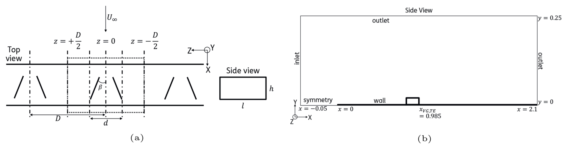
Figure 1 Sketch of (a) VG array geometry with simulation domain in dotted lines and (b) imposed boundary conditions. All coordinates are in metres.

The steady, incompressible, fully turbulent Reynolds-averaged Navier–Stokes (RANS) simulations are performed with a Spalart–Almaras (SA) turbulence model (Spalart and Allmaras, 1992) for the no-VG and VG setups. The single-equation SA turbulence model is chosen for its simplicity and relative insensitivity to grid resolution compared to other models (Bardina et al., 1997). While the SA model can underpredict skin friction for certain flows with lower Re_θ (Spalart and Garbaruk, 2020), it is accurate for the high range of Re_θ investigated in this study. Streamwise Reynolds numbers ${\mathit{Re}}_x=\mathrm{1}-\mathrm{10}\times {\mathrm{10}}^{\mathrm{6}}$ m⁻¹, corresponding to an incoming flow with Re_θ=2000–14 000 at the VG leading-edge location, were simulated. The results from ${\mathit{Re}}_x=\mathrm{2}\times {\mathrm{10}}^{\mathrm{6}}$ m⁻¹ are used to illustrate the derivation of new IBL equations in this work.

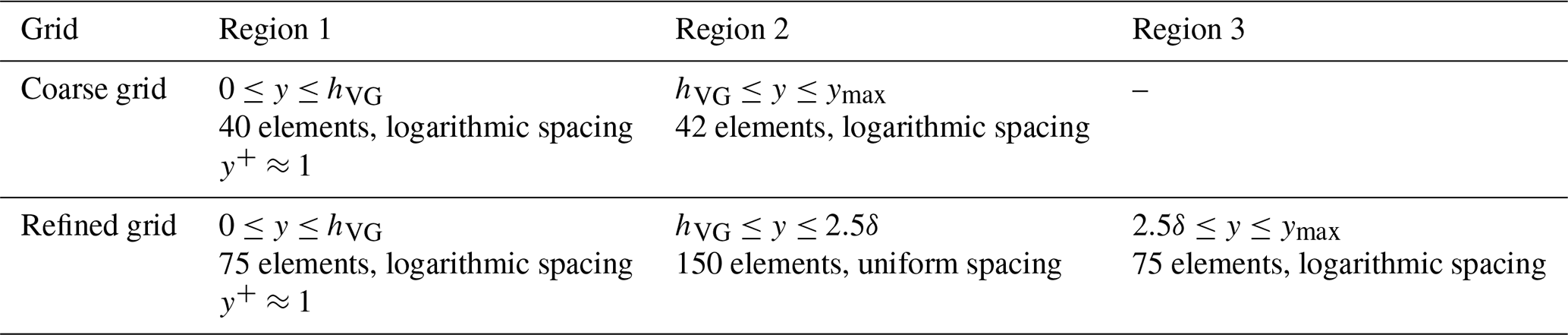
The simulation grid and boundary conditions are adapted for 3D periodic VG simulations from the incompressible turbulent flat-plate test case from the SU2 repository (Economon, 2018), which is in turn adapted from the test case described in the NASA turbulence modelling resource (Rumsey et al., 2010). The grid is adapted with additional refinement to better capture near-VG and near-wall effects. The coarse grid has $\mathrm{415}\times \mathrm{82}\times \mathrm{40}$ elements in the streamwise (X), wall-normal (Y), and spanwise (Z) directions. The refined grid has $\mathrm{500}\times \mathrm{300}\times \mathrm{40}$ elements, with mesh refinement near the VG location and in the boundary layer. The mesh refinement in the boundary layer is sketched in Fig. 2 and detailed in Table 1. A constant velocity inlet and constant pressure outlets bind the simulation domain. The VGs and the flat plate are prescribed as adiabatic no-slip walls. The surfaces at $z=\pm D/\mathrm{2}$ are prescribed with periodic boundary conditions.

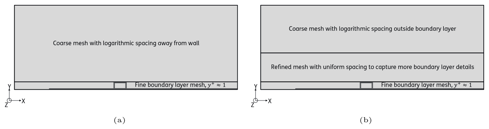
Figure 2 Schematic of (a) coarse mesh with around 1.4 million elements and (b) fine mesh with around 6 million elements to better capture the flow details in the boundary layer.

Table 1 Comparison of the coarse and refined grids in the Y direction (normal to the wall).

4 Modified IBL equations for VGs

Boundary layer data from the CFD simulations described in Sect. 3 were used to calculate all the VG and no-VG (integral) boundary layer quantities and modelling parameters presented in this section. Since this paper focuses on a VG model derived from the mean flow quantities, the modifications to Eqs. (1)–(2) form the focus of the paper. Like the original IBL equations, the VG IBL equations can be derived from the boundary layer equations that result from the changes in the mean flow of the turbulent boundary layers due to the streamwise vortices produced by the VGs.

4.1 Deriving the modified IBL equations for VGs

The steady incompressible boundary layer equations for flat plates equipped with VGs are given in Eqs. (4)–(6). The “–” over the velocities denotes the mean flow velocity components. The streamwise vortices released by the vortex generators introduce significant normal and spanwise velocities and gradients that cannot be neglected in the boundary layer equations. Consequently, unlike in the no-VG boundary layer, pressure is not invariant in the boundary layer in the normal direction and cannot be expressed in terms of the velocity outside the edge of the boundary layer U_e, as shown in Eq. (8). For the VG case, the streamwise pressure gradient in the boundary layer can be decomposed into an external flow contribution $\frac{\partial p_{\mathrm{e}}}{\partial x}$ and a VG contribution $\frac{\partial p_{i,\mathrm{VG}}}{\partial x}$, as shown in Eq. (9). Thus, the final continuity and X-momentum equations for VG boundary layers can be expressed as in Eqs. (10)–(11) and are used to derive the IBL equations.

$$\begin{array}{}\text{(4)}& {\displaystyle }\text{Continuity Equation:}{\displaystyle \frac{\partial \stackrel{\mathrm{‾}}{u}}{\partial x}}+{\displaystyle \frac{\partial \stackrel{\mathrm{‾}}{v}}{\partial y}}+{\displaystyle \frac{\partial \stackrel{\mathrm{‾}}{w}}{\partial z}}=\mathrm{0}\text{(5)}& {\displaystyle }\begin{array}{rl}X\text{Momentum Equation:}& \stackrel{\mathrm{‾}}{u}{\displaystyle \frac{\partial \stackrel{\mathrm{‾}}{u}}{\partial x}}+\stackrel{\mathrm{‾}}{v}{\displaystyle \frac{\partial \stackrel{\mathrm{‾}}{u}}{\partial y}}+\stackrel{\mathrm{‾}}{w}{\displaystyle \frac{\partial \stackrel{\mathrm{‾}}{u}}{\partial z}}\\ & =-{\displaystyle \frac{\mathrm{1}}{\mathit{\rho }}}{\displaystyle \frac{\partial p}{\partial x}}+{\displaystyle \frac{\mathrm{1}}{\mathit{\rho }}}\left({\displaystyle \frac{\partial {\mathit{\tau }}_{yx}}{\partial y}}+{\displaystyle \frac{\partial {\mathit{\tau }}_{zx}}{\partial z}}\right)\end{array}\text{(6)}& {\displaystyle }\begin{array}{rl}Y\text{Momentum Equation:}& \stackrel{\mathrm{‾}}{u}{\displaystyle \frac{\partial \stackrel{\mathrm{‾}}{v}}{\partial x}}+\stackrel{\mathrm{‾}}{v}{\displaystyle \frac{\partial \stackrel{\mathrm{‾}}{v}}{\partial y}}+\stackrel{\mathrm{‾}}{w}{\displaystyle \frac{\partial \stackrel{\mathrm{‾}}{v}}{\partial z}}\\ & =-{\displaystyle \frac{\mathrm{1}}{\mathit{\rho }}}{\displaystyle \frac{\partial p}{\partial y}}+{\displaystyle \frac{\mathrm{1}}{\mathit{\rho }}}\left({\displaystyle \frac{\partial {\mathit{\tau }}_{xy}}{\partial x}}+{\displaystyle \frac{\partial {\mathit{\tau }}_{zy}}{\partial z}}\right)\end{array}\text{(7)}& {\displaystyle }\begin{array}{rl}Z\text{Momentum Equation:}& \stackrel{\mathrm{‾}}{u}{\displaystyle \frac{\partial \stackrel{\mathrm{‾}}{w}}{\partial x}}+\stackrel{\mathrm{‾}}{v}{\displaystyle \frac{\partial \stackrel{\mathrm{‾}}{w}}{\partial y}}+\stackrel{\mathrm{‾}}{w}{\displaystyle \frac{\partial \stackrel{\mathrm{‾}}{w}}{\partial z}}\\ & =-{\displaystyle \frac{\mathrm{1}}{\mathit{\rho }}}{\displaystyle \frac{\partial p}{\partial z}}+{\displaystyle \frac{\mathrm{1}}{\mathit{\rho }}}\left({\displaystyle \frac{\partial {\mathit{\tau }}_{xz}}{\partial x}}+{\displaystyle \frac{\partial {\mathit{\tau }}_{yz}}{\partial y}}\right)\end{array}\text{(8)}& {\displaystyle }\begin{array}{rl}\text{In the no-VG boundary layer:}& {\displaystyle \frac{\partial p}{\partial y}}\approx \mathrm{0}\Rightarrow {\displaystyle \frac{\partial p}{\partial x}}\approx {\displaystyle \frac{d{p}_e}{\mathrm{d}x}}\\ & =-{\mathit{\rho }}_e{U}_{\mathrm{e}}{\displaystyle \frac{d{U}_{\mathrm{e}}}{\mathrm{d}x}}\end{array}\text{(9)}& {\displaystyle }\begin{array}{rl}\text{In the VG boundary layer:}& p=p_{\mathrm{e}}+p_{i,\mathrm{VG}}\Rightarrow {\displaystyle \frac{\partial p}{\partial x}}\\ & ={\displaystyle \frac{\partial p_{\mathrm{e}}}{\partial x}}+{\displaystyle \frac{\partial p_{i,\mathrm{VG}}}{\partial x}}\\ & =-\mathit{\rho }{U}_{\mathrm{e}}{\displaystyle \frac{\mathrm{d}{U}_{\mathrm{e}}}{\mathrm{d}x}}+{\displaystyle \frac{\partial p_{i,\mathrm{VG}}}{\partial x}}\end{array}\text{(10)}& {\displaystyle }\text{Continuity Equation:}{\displaystyle \frac{\partial \stackrel{\mathrm{‾}}{u}}{\partial x}}+{\displaystyle \frac{\partial \stackrel{\mathrm{‾}}{v}}{\partial y}}+{\displaystyle \frac{\partial \stackrel{\mathrm{‾}}{w}}{\partial z}}=\mathrm{0}\text{(11)}& {\displaystyle }\begin{array}{rl}X\text{Momentum Equation:}& \stackrel{\mathrm{‾}}{u}{\displaystyle \frac{\partial \stackrel{\mathrm{‾}}{u}}{\partial x}}+\stackrel{\mathrm{‾}}{v}{\displaystyle \frac{\partial \stackrel{\mathrm{‾}}{u}}{\partial y}}+\stackrel{\mathrm{‾}}{w}{\displaystyle \frac{\partial \stackrel{\mathrm{‾}}{u}}{\partial z}}\\ & =U_{\mathrm{e}}{\displaystyle \frac{\mathrm{d}{U}_{\mathrm{e}}}{\mathrm{d}x}}-{\displaystyle \frac{\mathrm{1}}{\mathit{\rho }}}{\displaystyle \frac{\partial p_{i,\mathrm{VG}}}{\partial x}}\\ & +{\displaystyle \frac{\mathrm{1}}{\mathit{\rho }}}\left({\displaystyle \frac{\partial {\mathit{\tau }}_{yx}}{\partial y}}+{\displaystyle \frac{\partial {\mathit{\tau }}_{zx}}{\partial z}}\right)\end{array}\end{array}$$

The IBL equations are calculated by taking the nth moment of the X-momentum equation and integrating along the boundary layer direction, as shown in Eq. (12). n=0 gives the IBL momentum equation, and n=1 gives the IBL kinetic energy equation.

$$\begin{array}{}\text{(12)}& \begin{array}{rl}{u}^n(n+\mathrm{1})& \left(\text{X Momentum equation}\right)-\left(U_{\mathrm{e}}^{n+\mathrm{1}}-u^{n+\mathrm{1}}\right)\\ & \left(\text{Continuity Equation}\right),n=\mathrm{0},\mathrm{1}\end{array}\end{array}$$

The integral form of the moment form is obtained by integrating Eq. (12) along the boundary layer direction, which then gives the integral boundary layer (IBL) form, as shown in Eq. (13). The order of the boundary layer equations is reduced by solving for the evolution of integral quantities in the streamwise direction instead of solving for the evolution of velocities and stresses in all directions of the boundary layer. To formulate the IBL equations for the VG case, the same principle is applied, but the variation in the span is also reduced through spanwise averaging. Thus, the system of equations is integrated both along the boundary layer height and the span, as shown in Eq. (14), to obtain the spanwise-averaged integral boundary layer equations for VGs. Since the pair of vortices from the VGs is counter-rotating, the spanwise flow is periodic along the span of a repeating VG pair unit. The domain for the spanwise integral is thus set to the space within one repeating VG pair unit.

$$\begin{array}{}\text{(13)}& {\displaystyle }\begin{array}{rl}& \text{IBL equations for no-VG case:}\\ & \underset{\mathrm{0}}{\overset{\mathit{\delta }}{\int }}\left(u^n\right(n+\mathrm{1})\left(\text{X Momentum equation}\right)\\ & -\left(U_{\mathrm{e}}^{n+\mathrm{1}}-u^{n+\mathrm{1}}\right)\left(\text{Continuity Equation}\right))\mathrm{d}y\end{array}\text{(14)}& {\displaystyle }\begin{array}{rl}& \text{IBL equations for VG case:}\\ & {\displaystyle \frac{\begin{array}{c}{\int }_{-D/\mathrm{2}}^{D/\mathrm{2}}{\int }_{\mathrm{0}}^{\mathit{\delta }}\left(u^n\right(n+\mathrm{1})\left(\text{X Momentum equation}\right)\\ -\left(U_{\mathrm{e}}^{n+\mathrm{1}}-u^{n+\mathrm{1}}\right)\left(\text{Continuity Equation}\right))\mathrm{d}y\mathrm{d}z\end{array}}{\underset{-D/\mathrm{2}}{\overset{D/\mathrm{2}}{\int }}\mathrm{d}z}}\end{array}\end{array}$$

Substituting n=0 and n=1 in Eq. (14) gives the IBL momentum and kinetic energy equations, respectively, for the VG case.

$$\begin{array}{}\text{(15)}& {\displaystyle }\begin{array}{rl}& {\displaystyle \frac{\underset{-D/\mathrm{2}}{\overset{D/\mathrm{2}}{\int }}\underset{\mathrm{0}}{\overset{\mathit{\delta }}{\int }}\left(\left(u\frac{\partial u}{\partial x}+v\frac{\partial u}{\partial y}+w\frac{\partial u}{\partial z}\right)-\left(U_{\mathrm{e}}-u\right)\left(\frac{\partial u}{\partial x}+\frac{\partial v}{\partial y}+\frac{\partial w}{\partial z}\right)\right)\mathrm{d}y\mathrm{d}z}{\underset{-D/\mathrm{2}}{\overset{D/\mathrm{2}}{\int }}\mathrm{d}z}}\\ & ={\displaystyle \frac{\underset{-D/\mathrm{2}}{\overset{D/\mathrm{2}}{\int }}\underset{\mathrm{0}}{\overset{\mathit{\delta }}{\int }}\left(U_{\mathrm{e}}\frac{d{U}_{\mathrm{e}}}{\mathrm{d}x}-\frac{\mathrm{1}}{\mathit{\rho }}\frac{\partial p_{i,VG}}{\partial x}+\frac{\mathrm{1}}{\mathit{\rho }}\left(\frac{\partial {\mathit{\tau }}_{yx}}{\partial y}+\frac{\partial {\mathit{\tau }}_{zx}}{\partial z}\right)\right)\mathrm{d}y\mathrm{d}z}{\underset{-D/\mathrm{2}}{\overset{D/\mathrm{2}}{\int }}\mathrm{d}z}}\end{array}\text{(16)}& {\displaystyle }\begin{array}{rl}& {\displaystyle \frac{\underset{-D/\mathrm{2}}{\overset{D/\mathrm{2}}{\int }}\underset{\mathrm{0}}{\overset{\mathit{\delta }}{\int }}\left(\mathrm{2}u\left(u\frac{\partial u}{\partial x}+v\frac{\partial u}{\partial y}+w\frac{\partial u}{\partial z}\right)-\left(U_{\mathrm{e}}^{\mathrm{2}}-u^{\mathrm{2}}\right)\left(\frac{\partial u}{\partial x}+\frac{\partial v}{\partial y}+\frac{\partial w}{\partial z}\right)\right)\mathrm{d}y\mathrm{d}z}{\underset{-D/\mathrm{2}}{\overset{D/\mathrm{2}}{\int }}\mathrm{d}z}}\\ & ={\displaystyle \frac{\underset{-D/\mathrm{2}}{\overset{D/\mathrm{2}}{\int }}\underset{\mathrm{0}}{\overset{\mathit{\delta }}{\int }}\left(\mathrm{2}u\left(U_{\mathrm{e}}\frac{\partial U_{\mathrm{e}}}{\partial x}-\frac{\mathrm{1}}{\mathit{\rho }}\frac{\partial p_{i,VG}}{\partial x}+\frac{\mathrm{1}}{\mathit{\rho }}\left(\frac{\partial {\mathit{\tau }}_{yx}}{\partial y}+\frac{\partial {\mathit{\tau }}_{zx}}{\partial z}\right)\right)\right)\mathrm{d}y\mathrm{d}z}{\underset{-D/\mathrm{2}}{\overset{D/\mathrm{2}}{\int }}\mathrm{d}z}}\end{array}\end{array}$$

The new integrals introduced in the VG IBL equations can be rearranged and simplified with the help of results shown in Eqs. (17)–(20). The spanwise velocity w and the spanwise stress component τ_zx are zero on the spanwise bounding planes $z=\pm D/\mathrm{2}$, resulting in most of the integrals of the spanwise velocity and shear stress components reducing to zero. Only the integral of the dissipative form of the spanwise shear stress gradient shown in Eq. (21) reduces to a non-zero value. The process of simplifying the rest of the integrals remains the same as in the no-VG case.

$$\begin{array}{}\text{(17)}& {\displaystyle }\begin{array}{rl}& \underset{-D/\mathrm{2}}{\overset{D/\mathrm{2}}{\int }}\underset{\mathrm{0}}{\overset{\mathit{\delta }}{\int }}{\displaystyle \frac{\partial }{\partial z}}\left(w\left(U_{\mathrm{e}}-u\right)\right)\mathrm{d}y\mathrm{d}z\\ & =\underset{-D/\mathrm{2}}{\overset{D/\mathrm{2}}{\int }}{\displaystyle \frac{d}{\mathrm{d}z}}\left(\underset{\mathrm{0}}{\overset{\mathit{\delta }}{\int }}\left(w\left(U_{\mathrm{e}}-u\right)\right)\mathrm{d}y\right)\mathrm{d}z\\ & =\left(\underset{\mathrm{0}}{\overset{\mathit{\delta }}{\int }}w\left(U_{\mathrm{e}}-u\right)\mathrm{d}y\right){|}_{z=D/\mathrm{2}}\\ & -\left(\underset{\mathrm{0}}{\overset{\mathit{\delta }}{\int }}w\left(U_{\mathrm{e}}-u\right)\mathrm{d}y\right){|}_{z=-D/\mathrm{2}}=\mathrm{0}\end{array}\text{(18)}& {\displaystyle }\begin{array}{rl}& \underset{-D/\mathrm{2}}{\overset{D/\mathrm{2}}{\int }}\underset{\mathrm{0}}{\overset{\mathit{\delta }}{\int }}-{\displaystyle \frac{\mathrm{1}}{\mathit{\rho }}}{\displaystyle \frac{\partial {\mathit{\tau }}_{zx}}{\partial z}}\mathrm{d}y\mathrm{d}z\\ & =\underset{-D/\mathrm{2}}{\overset{D/\mathrm{2}}{\int }}{\displaystyle \frac{d}{\mathrm{d}z}}\left(\underset{\mathrm{0}}{\overset{\mathit{\delta }}{\int }}-{\displaystyle \frac{\mathrm{1}}{\mathit{\rho }}}{\mathit{\tau }}_{zx}\mathrm{d}y\right)\mathrm{d}z\\ & =\left(\underset{\mathrm{0}}{\overset{\mathit{\delta }}{\int }}-{\displaystyle \frac{\mathrm{1}}{\mathit{\rho }}}{\mathit{\tau }}_{zx}\mathrm{d}y\right){|}_{z=D/\mathrm{2}}\\ & -\left(\underset{\mathrm{0}}{\overset{\mathit{\delta }}{\int }}-{\displaystyle \frac{\mathrm{1}}{\mathit{\rho }}}{\mathit{\tau }}_{zx}\mathrm{d}y\right){|}_{z=-D/\mathrm{2}}=\mathrm{0}\end{array}\end{array}$$

$$\begin{array}{}\text{(19)}& {\displaystyle }\begin{array}{rl}& \underset{-D/\mathrm{2}}{\overset{D/\mathrm{2}}{\int }}\underset{\mathrm{0}}{\overset{\mathit{\delta }}{\int }}{\displaystyle \frac{\partial }{\partial z}}\left(w\left(U_{\mathrm{e}}^{\mathrm{2}}-u^{\mathrm{2}}\right)\right)\mathrm{d}y\mathrm{d}z\\ & =\underset{-D/\mathrm{2}}{\overset{D/\mathrm{2}}{\int }}{\displaystyle \frac{d}{dz}}\left(\underset{\mathrm{0}}{\overset{\mathit{\delta }}{\int }}\left(w\left(U_{\mathrm{e}}^{\mathrm{2}}-u^{\mathrm{2}}\right)\right)\mathrm{d}y\right)\mathrm{d}z\\ & =\left(\underset{\mathrm{0}}{\overset{\mathit{\delta }}{\int }}w\left(U_{\mathrm{e}}^{\mathrm{2}}-u^{\mathrm{2}}\right)\mathrm{d}y\right){|}_{z=D/\mathrm{2}}\\ & -\left(\underset{\mathrm{0}}{\overset{\mathit{\delta }}{\int }}w\left(U_{\mathrm{e}}^{\mathrm{2}}-u^{\mathrm{2}}\right)\mathrm{d}y\right){|}_{z=-D/\mathrm{2}}=\mathrm{0}\end{array}\text{(20)}& {\displaystyle }\begin{array}{rl}& \underset{-D/\mathrm{2}}{\overset{D/\mathrm{2}}{\int }}\underset{\mathrm{0}}{\overset{\mathit{\delta }}{\int }}-{\displaystyle \frac{\mathrm{1}}{\mathit{\rho }}}{\displaystyle \frac{\partial }{\partial z}}\left(u{\mathit{\tau }}_{zx}\right)\mathrm{d}y\mathrm{d}z\\ & =\underset{-D/\mathrm{2}}{\overset{D/\mathrm{2}}{\int }}{\displaystyle \frac{d}{\mathrm{d}z}}\left(\underset{\mathrm{0}}{\overset{\mathit{\delta }}{\int }}-{\displaystyle \frac{\mathrm{1}}{\mathit{\rho }}}u{\mathit{\tau }}_{zx}\mathrm{d}y\right)\mathrm{d}z\\ & =\left(\underset{\mathrm{0}}{\overset{\mathit{\delta }}{\int }}-{\displaystyle \frac{\mathrm{1}}{\mathit{\rho }}}u{\mathit{\tau }}_{zx}\mathrm{d}y\right){|}_{z=D/\mathrm{2}}\\ & -\left(\underset{\mathrm{0}}{\overset{\mathit{\delta }}{\int }}-{\displaystyle \frac{\mathrm{1}}{\mathit{\rho }}}u{\mathit{\tau }}_{zx}\mathrm{d}y\right){|}_{z=-D/\mathrm{2}}=\mathrm{0}\end{array}\text{(21)}& {\displaystyle }\underset{-D/\mathrm{2}}{\overset{D/\mathrm{2}}{\int }}\underset{\mathrm{0}}{\overset{\mathit{\delta }}{\int }}{\displaystyle \frac{\mathrm{2}}{\mathit{\rho }}}{\mathit{\tau }}_{zx}{\displaystyle \frac{\partial u}{\partial z}}\mathrm{d}y\mathrm{d}z\ne \mathrm{0}\end{array}$$

This gives the IBL momentum equation (Eq. 22) and the IBL kinetic energy equation (Eq. 23). The new terms appearing due to VGs are highlighted. All pre-existing IBL quantities from the no-VG form have their usual meanings. A “–” over a quantity refers to its spanwise-averaged form.

$$\begin{array}{}\text{(22)}& {\displaystyle \frac{\mathrm{d}\stackrel{\mathrm{‾}}{\mathit{\theta }}}{\mathrm{d}x}}={\displaystyle \frac{\stackrel{\mathrm{‾}}{C_{\mathrm{f}}}}{\mathrm{2}}}-\left(\stackrel{\mathrm{‾}}{H}+\mathrm{2}\right){\displaystyle \frac{\stackrel{\mathrm{‾}}{\mathit{\theta }}}{U_{\mathrm{e}}}}{\displaystyle \frac{\mathrm{d}{U}_{\mathrm{e}}}{\mathrm{d}x}}+{\displaystyle \frac{\mathrm{1}}{\mathit{\rho }{U}_{\mathrm{e}}^{\mathrm{2}}}}\stackrel{\mathrm{‾}}{\left(\underset{\mathrm{0}}{\overset{\mathrm{\infty }}{\int }}{\displaystyle \frac{\partial p_{i,\mathrm{VG}}}{\partial x}}\mathrm{d}y\right)}\text{(23)}& {\displaystyle }\begin{array}{rl}{\displaystyle \frac{\mathrm{d}\stackrel{\mathrm{‾}}{H^{*}}}{\mathrm{d}x}}& =\mathrm{2}{\displaystyle \frac{\stackrel{\mathrm{‾}}{C_{\mathcal{D}}}}{\stackrel{\mathrm{‾}}{\mathit{\theta }}}}-{\displaystyle \frac{\stackrel{\mathrm{‾}}{H^{*}}}{\stackrel{\mathrm{‾}}{\mathit{\theta }}}}{\displaystyle \frac{\stackrel{\mathrm{‾}}{C_{\mathrm{f}}}}{\mathrm{2}}}+\left(\stackrel{\mathrm{‾}}{H}-\mathrm{1}\right){\displaystyle \frac{\stackrel{\mathrm{‾}}{H^{*}}}{U_{\mathrm{e}}}}{\displaystyle \frac{\mathrm{d}{U}_{\mathrm{e}}}{\mathrm{d}x}}\\ & +{\displaystyle \frac{\mathrm{2}}{\mathit{\rho }{U}_{\mathrm{e}}^{\mathrm{3}}\stackrel{\mathrm{‾}}{\mathit{\theta }}}}\stackrel{\mathrm{‾}}{\left(\underset{\mathrm{0}}{\overset{\mathit{\delta }}{\int }}{\mathit{\tau }}_{zx}{\displaystyle \frac{\partial u}{\partial z}}\mathrm{d}y\right)}\\ & +{\displaystyle \frac{\mathrm{2}}{\mathit{\rho }{U}_{\mathrm{e}}^{\mathrm{3}}}}\stackrel{\mathrm{‾}}{\left(\underset{\mathrm{0}}{\overset{\mathit{\delta }}{\int }}u{\displaystyle \frac{\partial p_{i,\mathrm{VG}}}{\partial x}}\mathrm{d}y\right)}\end{array}\end{array}$$

The IBL momentum equation for counter-rotating VGs is identical to the equation for without VGs except for the local induced velocity/pressure contribution from the vortices. The increased momentum in the boundary layer is implicitly modelled in the increased shape factor and the increased skin friction coefficient. The IBL kinetic energy equation (Eq. 23) has two additional terms – the term resulting from the local induced velocity contribution from the vortices and a dissipative term from the spanwise shear stress. This dissipative term can be interpreted as the additional kinetic energy added by the streamwise vortices due to the VGs to entrain higher-momentum flow from the upper parts of the boundary layer downward. Unlike the spanwise stresses themselves, the increase in kinetic energy due to the spanwise stresses does not cancel out over the span of one VG pair and is seen as a net dissipation term in the spanwise averaged equation. The term has a form similar to the already-existing viscous dissipation term C_𝒟 from the no-VG boundary layers, as illustrated in Eq. 24. Thus, we denote the term as C_𝒟z to denote that it arrives from the spanwise stresses.

$$\begin{array}{}\text{(24)}& \begin{array}{rl}& C_{\mathcal{D}}={\displaystyle \frac{\mathrm{1}}{\mathit{\rho }{U}_{\mathrm{e}}^{\mathrm{3}}}}\underset{\mathrm{0}}{\overset{\mathit{\delta }}{\int }}\left({\mathit{\tau }}_{yx}{\displaystyle \frac{\partial u}{\partial y}}\right)\mathrm{d}y,\\ & C_{\mathcal{D}z}={\displaystyle \frac{\mathrm{1}}{\mathit{\rho }{U}_{\mathrm{e}}^{\mathrm{3}}}}\underset{\mathrm{0}}{\overset{\mathit{\delta }}{\int }}\left({\mathit{\tau }}_{zx}{\displaystyle \frac{\partial u}{\partial z}}\right)\mathrm{d}y\end{array}\end{array}$$

Hence, the final form of the IBL equations for incompressible turbulent span-averaged boundary layers due to counter-rotating VGs with a common downwash is

$$\begin{array}{}\text{(25)}& {\displaystyle \frac{\mathrm{d}\stackrel{\mathrm{‾}}{\mathit{\theta }}}{\mathrm{d}x}}={\displaystyle \frac{\stackrel{\mathrm{‾}}{C_{\mathrm{f}}}}{\mathrm{2}}}-\left(\stackrel{\mathrm{‾}}{H}+\mathrm{2}\right){\displaystyle \frac{\stackrel{\mathrm{‾}}{\mathit{\theta }}}{U_{\mathrm{e}}}}{\displaystyle \frac{\mathrm{d}{U}_{\mathrm{e}}}{\mathrm{d}x}}+{\displaystyle \frac{\mathrm{1}}{\mathit{\rho }{U}_{\mathrm{e}}^{\mathrm{2}}}}\stackrel{\mathrm{‾}}{\left(\underset{\mathrm{0}}{\overset{\mathrm{\infty }}{\int }}{\displaystyle \frac{\partial p_{i,\mathrm{VG}}}{\partial x}}\mathrm{d}y\right),}\text{(26)}& {\displaystyle }\begin{array}{rl}{\displaystyle \frac{\mathrm{d}\stackrel{\mathrm{‾}}{H^{*}}}{\mathrm{d}x}}& =\mathrm{2}{\displaystyle \frac{\stackrel{\mathrm{‾}}{C_{\mathcal{D}}}}{\stackrel{\mathrm{‾}}{\mathit{\theta }}}}-{\displaystyle \frac{\stackrel{\mathrm{‾}}{H^{*}}}{\stackrel{\mathrm{‾}}{\mathit{\theta }}}}{\displaystyle \frac{\stackrel{\mathrm{‾}}{C_{\mathrm{f}}}}{\mathrm{2}}}+\left(\stackrel{\mathrm{‾}}{H}-\mathrm{1}\right){\displaystyle \frac{\stackrel{\mathrm{‾}}{H^{*}}}{U_{\mathrm{e}}}}{\displaystyle \frac{\mathrm{d}{U}_{\mathrm{e}}}{\mathrm{d}x}}\\ & +{\displaystyle \frac{\mathrm{2}\stackrel{\mathrm{‾}}{C_{\mathcal{D}z}}}{\stackrel{\mathrm{‾}}{\mathit{\theta }}}}+{\displaystyle \frac{\mathrm{2}}{\mathit{\rho }{U}_{\mathrm{e}}^{\mathrm{3}}}}\stackrel{\mathrm{‾}}{\left(\underset{\mathrm{0}}{\overset{\mathit{\delta }}{\int }}u{\displaystyle \frac{\partial p_{i,\mathrm{VG}}}{\partial x}}\mathrm{d}y\right).}\end{array}\end{array}$$

4.2 A note on spanwise averaging

The IBL equations described in subsequent sections are expressed in terms of the spanwise-averaged form of all the IBL quantities, which are henceforth denoted with a “–”. The VG model proposed in this paper is thus limited to predicting the 2D boundary layer characteristics and force coefficients representing the average aerodynamic behaviour in the span.

All spanwise-averaged quantities in this paper are averaged along the span of a repeating VG pair unit in an array of counter-rotating VG vanes (sketched in Fig. 1a), as described in Eq. (27). For IBL quantities that are defined as ratios of other IBL quantities (e.g. the shape factors H and H^*), the spanwise-averaged form is taken as the spanwise average of the ratio. For example, the spanwise-averaged H, a ratio of δ^* to θ, is shown in Eq. (28). For the zero-pressure gradient flat-plate boundary layers, it was verified that both definitions approximately yield the same value; i.e. $\stackrel{\mathrm{‾}}{\left(\frac{{\mathit{\delta }}^{*}}{\mathit{\theta }}\right)}\approx \frac{\stackrel{\mathrm{‾}}{{\mathit{\delta }}^{*}}}{\stackrel{\mathrm{‾}}{\mathit{\theta }}}$. However, this may not hold for boundary layers with different pressure gradients.

$$\begin{array}{}\text{(27)}& {\displaystyle }\text{For a VG IBL quantity }Q,\stackrel{\mathrm{‾}}{Q}={\displaystyle \frac{{\int }_{-D/\mathrm{2}}^{D/\mathrm{2}}Q\mathrm{d}z}{{\int }_{-D/\mathrm{2}}^{D/\mathrm{2}}\mathrm{d}z}}\text{(28)}& {\displaystyle }\text{For ratios such as}H,\stackrel{\mathrm{‾}}{H}=\stackrel{\mathrm{‾}}{\left({\displaystyle \frac{{\mathit{\delta }}^{*}}{\mathit{\theta }}}\right)}\ne {\displaystyle \frac{\stackrel{\mathrm{‾}}{{\mathit{\delta }}^{*}}}{\stackrel{\mathrm{‾}}{\mathit{\theta }}}}\end{array}$$

4.3 Verifying the validity of closure relations for VGs

Closures are additional relations accompanying the system of IBL equations to close the set of three equations solving for six unknowns – δ^*, θ, C_f, H^*, C_𝒟, and C_τ. The existing closure relations for each quantity for the no-VG case can be found in the literature (e.g. Drela, 1986). The closure relations were evaluated for the VG case using the CFD values of H and Re_θ, as described in Eqs. (29–31). Comparison between the VG and no-VG cases in Fig. 3 shows that the closures are still valid in predicting H^* and C_f to the same degree of accuracy for the VG case as they do for the no-VG case. For C_𝒟, the closure cannot capture the streamwise variation when only the normal viscous dissipation is considered. However, if the normal dissipation C_𝒟 and the spanwise dissipation C_𝒟z are added to obtain a total dissipation C_𝒟,total, as described in Eq. (32), then it can be seen in Fig. 3b that the sum of the C_𝒟 calculated from the closure relation and the C_𝒟z obtained from CFD adequately captures the total dissipation C_𝒟,total compared to the no-VG case.

$$\begin{array}{}\text{(29)}& {\displaystyle }{\stackrel{\mathrm{‾}}{H^{\ast }}}_{\mathrm{closure}}=f\left({\stackrel{\mathrm{‾}}{H}}_{\mathrm{CFD}},{\stackrel{\mathrm{‾}}{{\mathit{Re}}_{\mathit{\theta }}}}_{\mathrm{CFD}}\right)\text{(30)}& {\displaystyle }{\stackrel{\mathrm{‾}}{C_{\mathrm{f}}}}_{\mathrm{closure}}=f\left({\stackrel{\mathrm{‾}}{H}}_{\mathrm{CFD}},{\stackrel{\mathrm{‾}}{{\mathit{Re}}_{\mathit{\theta }}}}_{\mathrm{CFD}}\right)\text{(31)}& {\displaystyle }{\stackrel{\mathrm{‾}}{C_{\mathcal{D}}}}_{\mathrm{closure}}=f\left({\stackrel{\mathrm{‾}}{C_{\mathrm{f}}}}_{\mathrm{closure}},{\stackrel{\mathrm{‾}}{H^{\ast }}}_{\mathrm{closure}},{\stackrel{\mathrm{‾}}{C_{\mathit{\tau }}}}_{\mathrm{CFD}},{\stackrel{\mathrm{‾}}{H}}_{\mathrm{CFD}}\right)\text{(32)}& {\displaystyle }\stackrel{\mathrm{‾}}{C_{\mathcal{D},\mathrm{total}}}={\stackrel{\mathrm{‾}}{C_{\mathcal{D}}}}_{\mathrm{closure}}+{\stackrel{\mathrm{‾}}{C_{\mathcal{D}z}}}_{\mathrm{CFD}}\end{array}$$

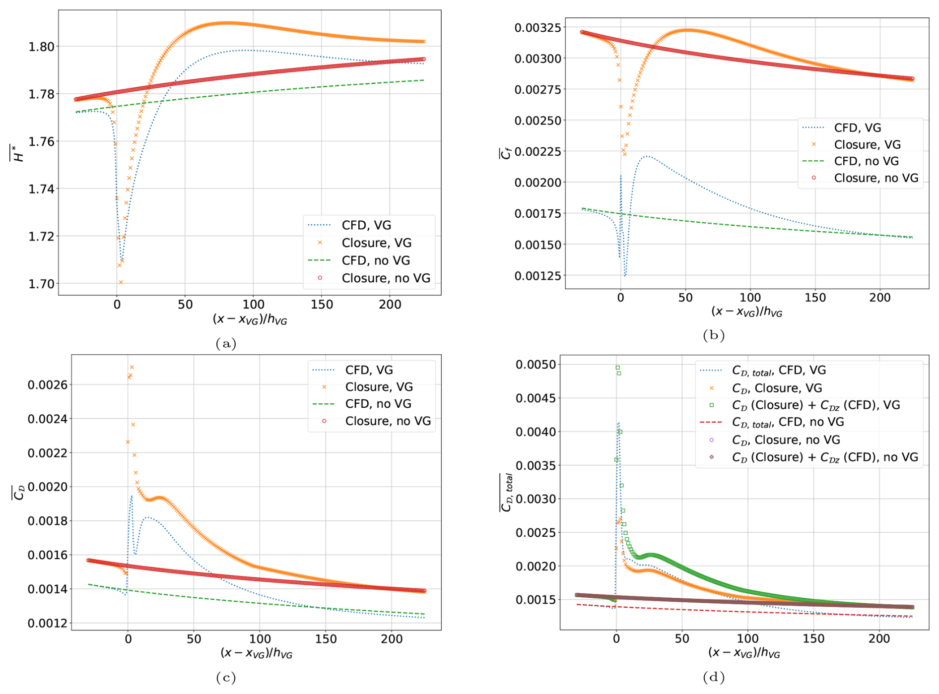
Figure 3 IBL quantities: (a) kinetic energy shape factor, (b) skin friction coefficient, (c) viscous dissipation coefficient, and (d) total viscous dissipation coefficient calculated with the closure relations compared to the CFD values at $R{e}_x=\mathrm{2}\times {\mathrm{10}}^{\mathrm{6}}$. The closures remain valid to a similar level of accuracy in the VG case as in the no-VG case. The viscous dissipation coefficient closure is accurate only when combined with the spanwise dissipation to obtain the total dissipation.

5 Modelling the VG IBL equations in RFOIL

5.1 Choosing the most significant VG IBL terms to model in RFOIL

The most significant changes in the new IBL equations for VGs are the modified shape factor $\stackrel{\mathrm{‾}}{H}$ and the additional viscous dissipation $\stackrel{\mathrm{‾}}{C_{\mathcal{D}z}}$, shown in Fig. 5. The rest of the spanwise-averaged IBL quantities, $\stackrel{\mathrm{‾}}{C_{\mathrm{f}}}$, $\stackrel{\mathrm{‾}}{H^{*}}$, and $\stackrel{\mathrm{‾}}{C_{\mathcal{D}}}$, can be calculated accurately through closure equations using $\stackrel{\mathrm{‾}}{H}$ and $\stackrel{\mathrm{‾}}{{\mathit{Re}}_{\mathit{\theta }}}$. The original closure equations are still valid for the VG case and are shown in Sect. 4.3 for completeness. While the induced pressure terms are significant near the VG, they quickly disappear within 10–15 heights downstream of the VG location (Fig. 4). Meanwhile, the significant VG-induced changes in the spanwise-averaged shape factor and dissipation coefficient can persist as far as 150–200 heights downstream of the VG location, as seen in Fig. 5. Moreover, the induced pressure terms can depend significantly on the boundary layer state, strength of the pressure gradient, separation, and so on, making it complex to model in a simple VG model with minimal parameters derived from flat-plate vortex dynamics. Thus, we focus on the shape factor and viscous dissipation in this paper's proposed VG model. In Sect. 5.2, we propose an analytical function dependent on the VG array geometry and Reynolds number to obtain the VG shape factor from the no-VG value. In Sect. 5.3, we model the total viscous dissipation as the sum of the dissipation obtained from the no-VG closure relation and a function dependent on the VG array geometry and Reynolds number to obtain the additional VG dissipation.

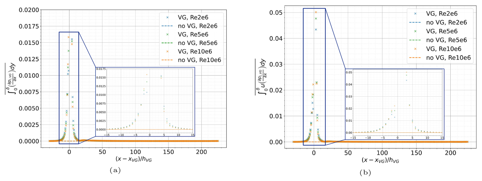
Figure 4 The induced pressure terms in (a) the momentum equation and (b) the kinetic energy equation are of a significant order of magnitude only in the near field of the VGs.

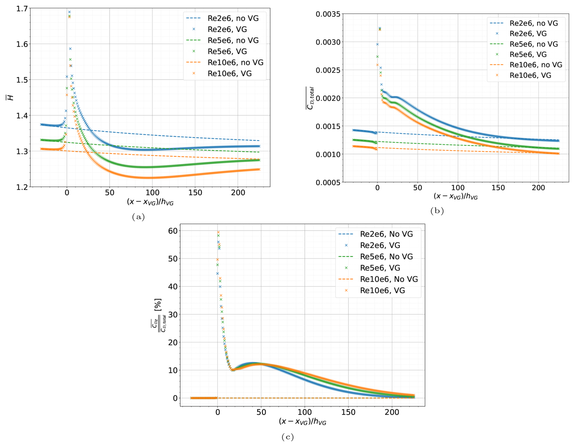
Figure 5 The VG and no-VG (a) shape factor and (b) total viscous dissipation coefficient compared for the flat plate with VG case described in Sect. 3. The spanwise viscous dissipation contributes to the total viscous dissipation in (c) up to 180 heights downstream of the VG location, while changes in the shape factor in (a) can persist more than 200 heights downstream of the VGs.

5.2 Modelling the shape factor

The distribution of the shape factor in the span of one counter-rotating VG pair is shown for a few downstream locations in Fig. 6. The global minima of the distribution remain constant in the span at the centre line z=0 between the two VG vanes. The peak locations move towards the symmetry lines $z=\pm D/\mathrm{2}$ as the vortices drift away from each other, directed by the vane placement and alignment.

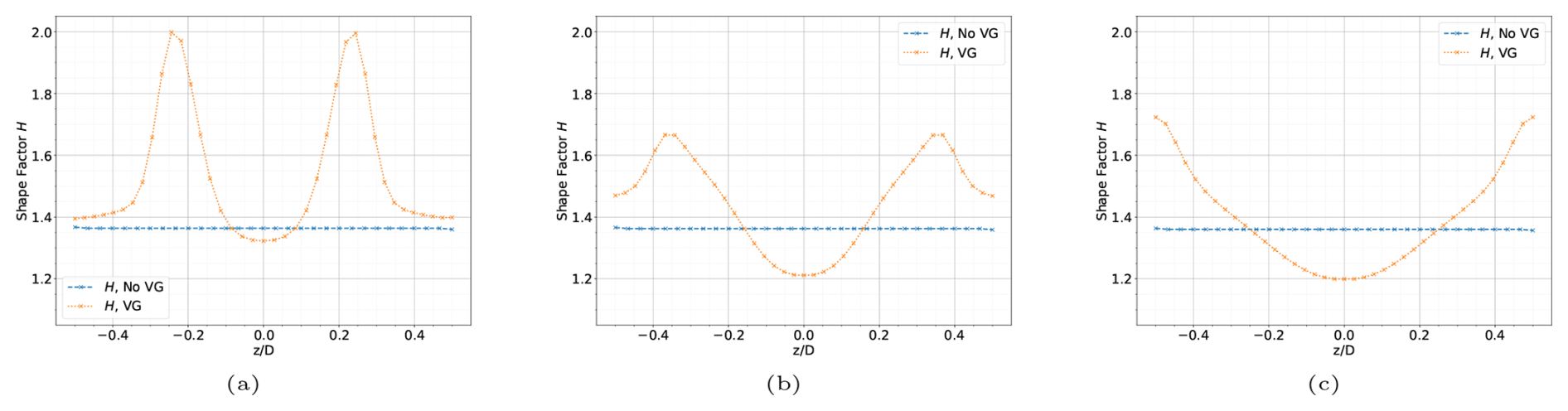
Figure 6 Distribution of the shape factor in the span shown for $\left(x-x_{\mathrm{VG}}\right)/h_{\mathrm{VG}}=$ (a) 5, (b) 10, and (c) 20 heights downstream of the VG location for a flat plate equipped with VGs of 5 mm height.

We can model this spanwise distribution by using the sum of two symmetric Gaussian distributions equidistant from the centreline z=0 between the two VG vanes. At any given streamwise location x, the expression for a Gaussian distribution as a function of the spanwise coordinate z is given by Eq. (33), where the centre μ(x) and the spread σ(x) are assumed to vary only in x. To obtain two Gaussian distributions symmetric about z=0, we can substitute the centre as ±μ(x) and get a function φ(x,z), as shown in Eq. (34). This function can be spanwise averaged with the limits $z=\pm D/\mathrm{2}$ to obtain the spanwise-averaged function $\stackrel{\mathrm{‾}}{\mathit{\phi }\left(x\right)}$, as shown in Eq. (35), where “erf” denotes the error function.

$$\begin{array}{}\text{(33)}& {\displaystyle }\begin{array}{rl}f\left(x,z\right)& ={\displaystyle \frac{\mathrm{1}}{\sqrt{\mathrm{2}\mathit{\pi }{\left(\mathit{\sigma }\left(x\right)\right)}^{\mathrm{2}}}}}\exp \left(-{\displaystyle \frac{{\left(z-\mathit{\mu }\left(x\right)\right)}^{\mathrm{2}}}{\mathrm{2}{\left(\mathit{\sigma }\left(x\right)\right)}^{\mathrm{2}}}}\right)\\ & ={\displaystyle \frac{\mathrm{1}}{\mathit{\sigma }\left(x\right)\sqrt{\mathrm{2}\mathit{\pi }}}}\exp \left(-{\displaystyle \frac{\mathrm{1}}{\mathrm{2}}}{\left({\displaystyle \frac{z-\mathit{\mu }\left(x\right)}{\mathit{\sigma }\left(x\right)}}\right)}^{\mathrm{2}}\right)\end{array}\text{(34)}& {\displaystyle }\begin{array}{rl}\mathit{\phi }\left(x,z\right)& ={\displaystyle \frac{\mathrm{1}}{\mathit{\sigma }\left(x\right)\sqrt{\mathrm{2}\mathit{\pi }}}}(\exp \left(-{\displaystyle \frac{\mathrm{1}}{\mathrm{2}}}{\left({\displaystyle \frac{z-\mathit{\mu }\left(x\right)}{\mathit{\sigma }\left(x\right)}}\right)}^{\mathrm{2}}\right)\\ & +\exp \left(-{\displaystyle \frac{\mathrm{1}}{\mathrm{2}}}{\left({\displaystyle \frac{z+\mathit{\mu }\left(x\right)}{\mathit{\sigma }\left(x\right)}}\right)}^{\mathrm{2}}\right))\end{array}\text{(35)}& {\displaystyle }\begin{array}{rl}\stackrel{\mathrm{‾}}{\mathit{\phi }\left(x\right)}& ={\displaystyle \frac{{\int }_{-D/\mathrm{2}}^{D/\mathrm{2}}\mathit{\phi }\left(x,z\right)\mathrm{d}z}{{\int }_{-D/\mathrm{2}}^{D/\mathrm{2}}\mathrm{d}z}}=\mathrm{erf}\left({\displaystyle \frac{\mathrm{0.5}-\mathit{\mu }\left(x\right)}{\mathit{\sigma }\left(x\right)\sqrt{\mathrm{2}}}}\right)\\ & +\mathrm{erf}\left({\displaystyle \frac{\mathrm{0.5}+\mathit{\mu }\left(x\right)}{\mathit{\sigma }\left(x\right)\sqrt{\mathrm{2}}}}\right)\end{array}\end{array}$$

To model the VG shape factor, we multiply the corresponding no-VG value by this transformation function $\stackrel{\mathrm{‾}}{\mathit{\phi }\left(x\right)}$, as shown in Eqs. (36)–(37). Some instances of using this transformation function on the flat-plate CFD data are shown in Fig. 7a–c at streamwise locations 5, 10, and 20 heights downstream of the VG location. This approximation deviates slightly from the actual shape in the span but accurately estimates the spanwise-averaged shape factor, as seen in Fig. 7d. Thus, the VG model in this work predicts the spanwise-averaged values of IBL quantities and cannot predict the accurate variation in IBL quantities in the span.

$$\begin{array}{}\text{(36)}& {\displaystyle }{H}_{\mathrm{VG}}\left(x,z\right)=H_{\mathrm{noVG}}\mathit{\phi }\left(x,z\right)\text{(37)}& {\displaystyle }\stackrel{\mathrm{‾}}{H_{\mathrm{VG}}\left(x\right)}=H_{\mathrm{noVG}}\stackrel{\mathrm{‾}}{\mathit{\phi }\left(x\right)}\end{array}$$

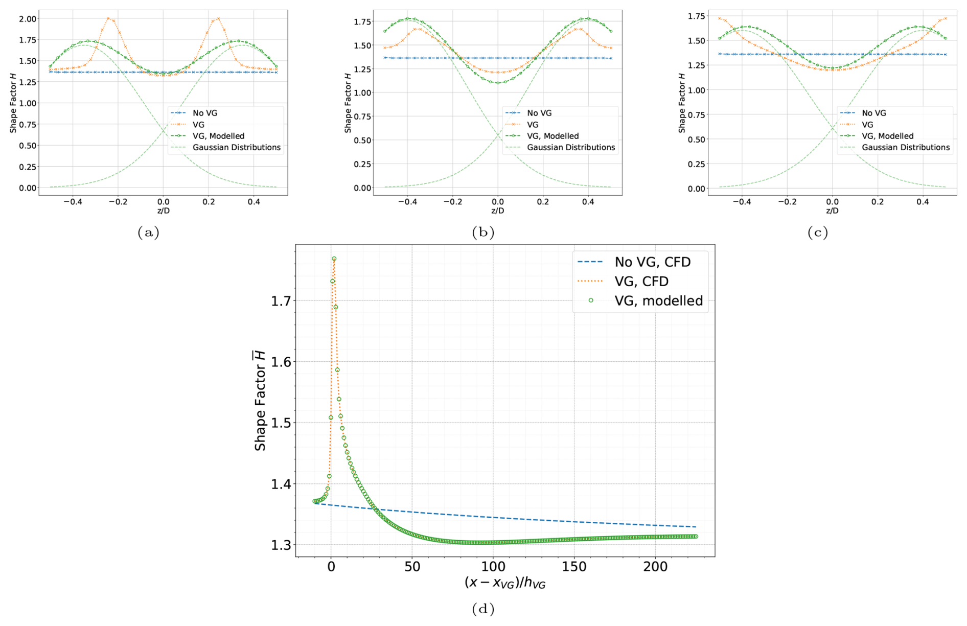
Figure 7 The CFD-predicted shape factor throughout the span compared to the approximation as the sum of two Gaussian distributions at $\left(x-x_{\mathrm{VG}}\right)/h_{\mathrm{VG}}=$ (a) 5, (b) 10, and (c) 20 heights downstream of the VG location for a flat plate equipped with VGs of 5 mm height at a Reynolds number of 2 million. The spanwise-averaged value is presented in (d).

To obtain this model in non-dimensional form, the streamwise coordinate x is converted to the relative distance to the VG location and scaled with the VG vane height as $\stackrel{\mathrm{̃}}{x}=(x-x_{\mathrm{VG}})/h_{\mathrm{VG}}$. The centre of the Gaussian distributions $\mathit{\mu }\left(\stackrel{\mathrm{̃}}{x}\right)$ is taken to follow a path downstream of the VG location directed by the orientation and placement of the VG vanes, as sketched in Fig. 8. The spread parameter of the Gaussian distributions $\mathit{\sigma }\left(\stackrel{\mathrm{̃}}{x}\right)$ is a function of the local Reynolds number Re_θ, as shown in Fig. 9. Both $\mathit{\mu }\left(\stackrel{\mathrm{̃}}{x}\right)$ and $\mathit{\sigma }\left(\stackrel{\mathrm{̃}}{x}\right)$ are also scaled with the spacing between VG pairs D to generalise the expressions for different VG array spacings.

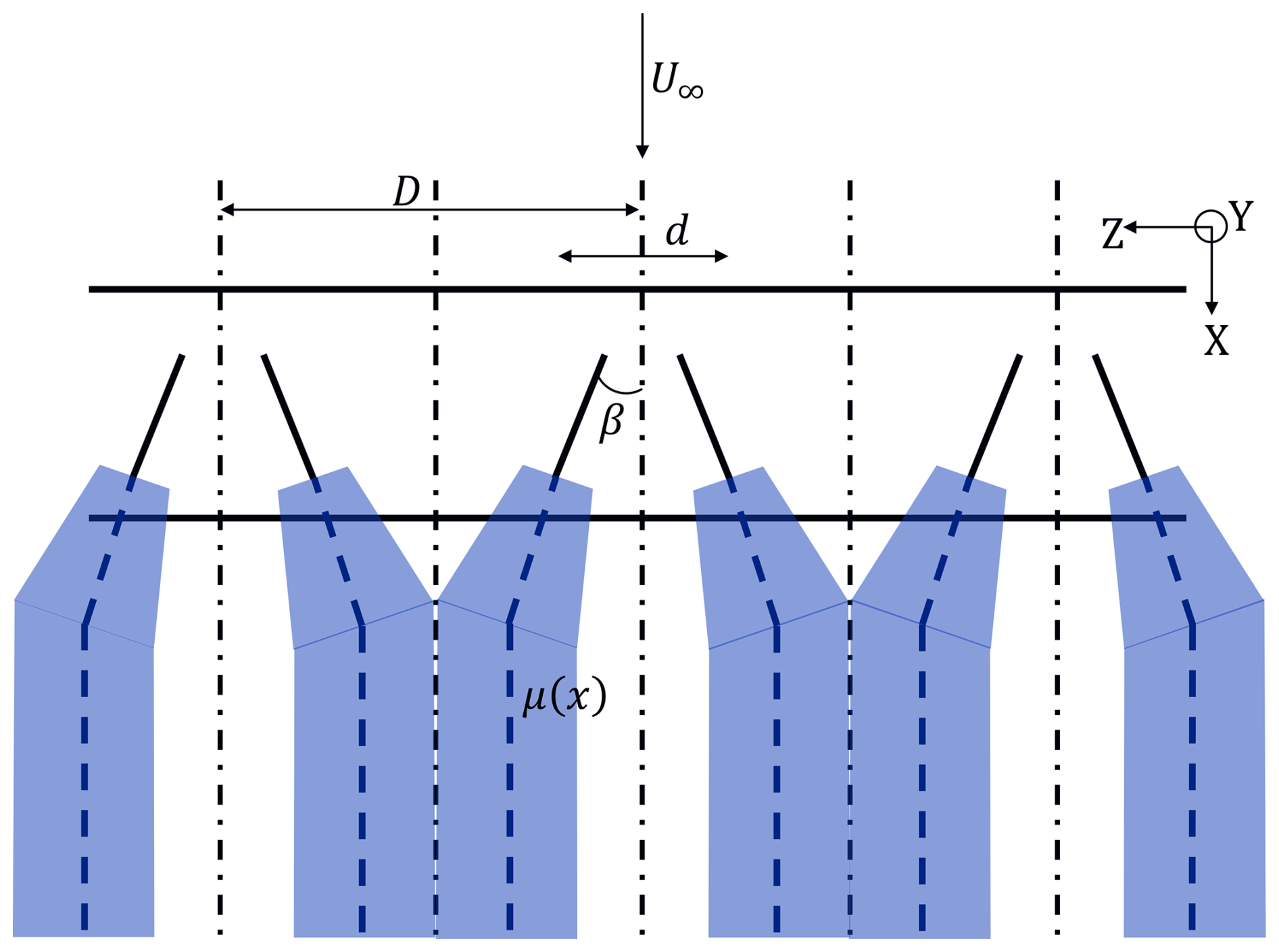
Figure 8 Visualising the distribution of the shape factor as the sum of Gaussian distributions in the X–Z plane. The centre of the distributions $\mathit{\mu }\left(\stackrel{\mathrm{̃}}{x}\right)$ is sketched with the dashed blue lines.

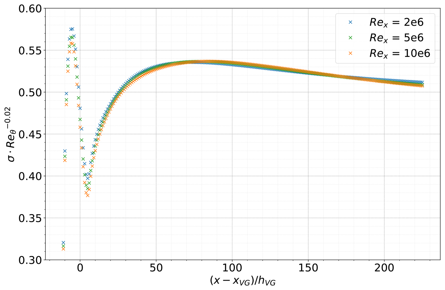
Figure 9 The spread parameter $\mathit{\sigma }\left(\stackrel{\mathrm{̃}}{x}\right)$ of the shape factor model is a function of the Reynolds number and the relative distance to the VG location scaled with the vane height.

5.3 Modelling the viscous dissipation coefficient

The total dissipation coefficient $\stackrel{\mathrm{‾}}{C_{\mathcal{D},\mathrm{total}}}=\stackrel{\mathrm{‾}}{C_{\mathcal{D}}}+\stackrel{\mathrm{‾}}{C_{\mathcal{D}z}}$ consists of the existing $\stackrel{\mathrm{‾}}{C_{\mathcal{D}}}$ and the additional VG contribution $\stackrel{\mathrm{‾}}{C_{\mathcal{D}z}}$. While verifying the closure equations in Sect. 4.3, it was verified that $\stackrel{\mathrm{‾}}{C_{\mathcal{D}}}$ can be calculated with the pre-existing no-VG closure equation if the correct shape factor and Reynolds number are used. Thus, only the new VG contribution $\stackrel{\mathrm{‾}}{C_{\mathcal{D}z}}$ needs to be modelled. Just like the σ parameter for the shape factor in Sect. 5.2, $\stackrel{\mathrm{‾}}{C_{\mathcal{D}z}}$ can also be expressed as a function of the VG height-scaled relative downstream location $\stackrel{\mathrm{̃}}{x}$ and $\stackrel{\mathrm{‾}}{{\mathit{Re}}_{\mathit{\theta }}}$, as shown in Fig. 10. Thus, the total viscous dissipation is modelled as described in Eq. (38), where the shape factor $\stackrel{\mathrm{‾}}{H}$ is modelled as described in Sect. 5.2.

$$\begin{array}{}\text{(38)}& \begin{array}{rl}& \stackrel{\mathrm{‾}}{C_{\mathcal{D},\mathrm{total}}}\left(\stackrel{\mathrm{̃}}{x},\mathit{Re}\right)={\stackrel{\mathrm{‾}}{C_{\mathcal{D}}}}_{\mathrm{closure}}\left(\stackrel{\mathrm{‾}}{H},\mathit{Re}\right)+\stackrel{\mathrm{‾}}{C_{\mathcal{D}z}}\left(\stackrel{\mathrm{̃}}{x},\mathit{Re}\right),\\ & \text{where}\stackrel{\mathrm{̃}}{x}={\displaystyle \frac{x-x_{\mathrm{VG}}}{h_{\mathrm{VG}}}}\end{array}\end{array}$$

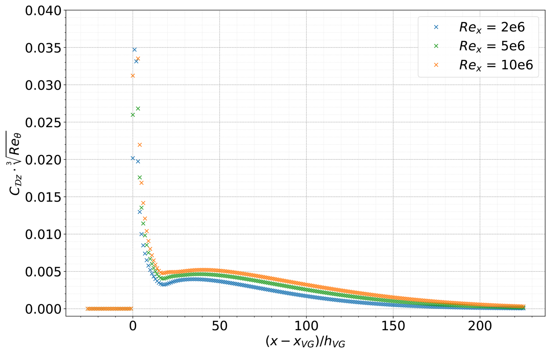
Figure 10 Additional viscous dissipation due to VGs C_𝒟z is a function of Reynolds number and the relative distance to the VG location scaled with the vane height.

5.4 Modelling transition to turbulence and upstream effects

Since VGs generally promote transition to turbulent flow, the previous VG models for IBL solvers (De Tavernier et al., 2018; Daniele et al., 2019) fixed the transition location at the VG location in case of an incoming laminar boundary layer. The VG calculations also started at the panel corresponding to the exact VG location. However, Fig. 5 – comparing the VG and no-VG shape factor and viscous dissipation coefficient – shows an upstream impact of the VGs, where the VG values start deviating from the clean values about 9 to 10 vane heights upstream of the VG location. To include the upstream effects, the proposed model makes two changes to the RFOIL IBL solver. First, the transition location x_tr is fixed to be at a panel 10 vane heights upstream of the VG location in case of incoming laminar flow, as described in Eq. (39). Secondly, the IBL solver switches to the VG IBL formulation one vane height downstream of the transition location, keeping a gap of at least a few panel lengths between the transition location and the location where VG calculations start. This has a twofold benefit. Firstly, including the upstream effects of the VGs in the IBL formulation improves the accuracy of the boundary layer calculations. Secondly, creating a gap of a few panels between the panel where the IBL solver switches to the turbulent formulation and the panel where the IBL solver switches to the VG formulation smoothens the streamwise gradients of the calculated IBL quantities by distributing the change in the IBL quantities over several panels. In contrast, the sharp change in IBL quantities over the distance of one single panel length calculated by RFOILVG often leads to sharp gradients and convergence issues. This improvement in convergence is discussed with examples of airfoil calculations in Sect. 8.2.

$$\begin{array}{}\text{(39)}& x_{\mathrm{tr}}=\left\{\begin{array}{l}{x}_{\mathrm{VG}}-\mathrm{10}{h}_{\mathrm{VG}},\text{if }{x}_{\mathrm{tr}}>\left(x_{\mathrm{VG}}-\mathrm{10}{h}_{\mathrm{VG}}\right)\\ x_{\mathrm{tr}},\text{otherwise}\end{array}\right.\end{array}$$

5.5 Flow separation check in the new VG model

XFOIL and RFOIL use the shape factor threshold method to determine if the boundary layer is separated. In XFOIL, flow separation is assumed to occur if the shape factor H exceeds a certain threshold value of 2.5 for laminar boundary layers and 3.8 for turbulent boundary layers, with RFOIL using similar threshold values (Van Rooij, 1996). The new VG model in RFOIL uses the existing method in no-VG RFOIL to determine flow separation. The validity of this method in the presence of VGs is verified in Sect. 7 using pressure distributions around the airfoil (wherever available) to compare the flow separation location between experimental data and RFOIL calculations.

6 Verification of the new VG model

The VG model implementation in RFOIL was verified by recreating the turbulent flat-plate CFD setup in RFOIL. The NASA SC(2)-0402 airfoil (Harris, 1990) with a maximum thickness-to-chord ratio of 2 % was chosen for this verification exercise. The aerodynamic properties of the airfoil were calculated in RFOIL at an angle of attack of 1° for a chordwise Reynolds number of 2 million with transition to turbulence forced at 5 % chordwise location on both sides of the airfoil. This gave an approximately zero pressure gradient on the upper surface downstream of the chordwise location $x/c=\mathrm{0.15}$ (as seen in Fig. 11a) and a boundary layer development that closely approximates the one seen on the turbulent flat plate in the CFD simulations (Fig. 11b). The VG case is recreated by placing a VG array of rectangular vanes at a chordwise location of $x/c=\mathrm{0.15}$ with the same array geometry parameters modelled in the CFD simulations.

Figure 11 The flat-plate zero-pressure gradient turbulent boundary layer from CFD simulations recreated in RFOIL with the NASA SC(2)-0402 airfoil at 1° angle of attack by (a) ensuring a zero-pressure gradient on the upper surface of the airfoil and (b) mimicking the flat-plate boundary layer growth on the airfoil upper surface.

The integral boundary layer properties calculated by RFOIL using the VG model are shown in Fig. 12. The RFOIL VG model calculations predict higher mixing due to VGs than the simulations. This is seen in the model's accurate prediction of the momentum thickness θ but underprediction of the displacement thickness δ^* in the near field of the VGs. However, the overall trend is captured well. The VGs produce a larger relative increase in the momentum thickness than the displacement thickness, resulting in a lower shape factor downstream of the VGs. A lower shape factor than expected means that the model overestimates the mixing produced by VGs compared to CFD calculations. This is also reflected in the secondary IBL parameters like skin friction and total viscous dissipation. A lower shape factor estimation results in higher skin friction and viscous dissipation estimates.

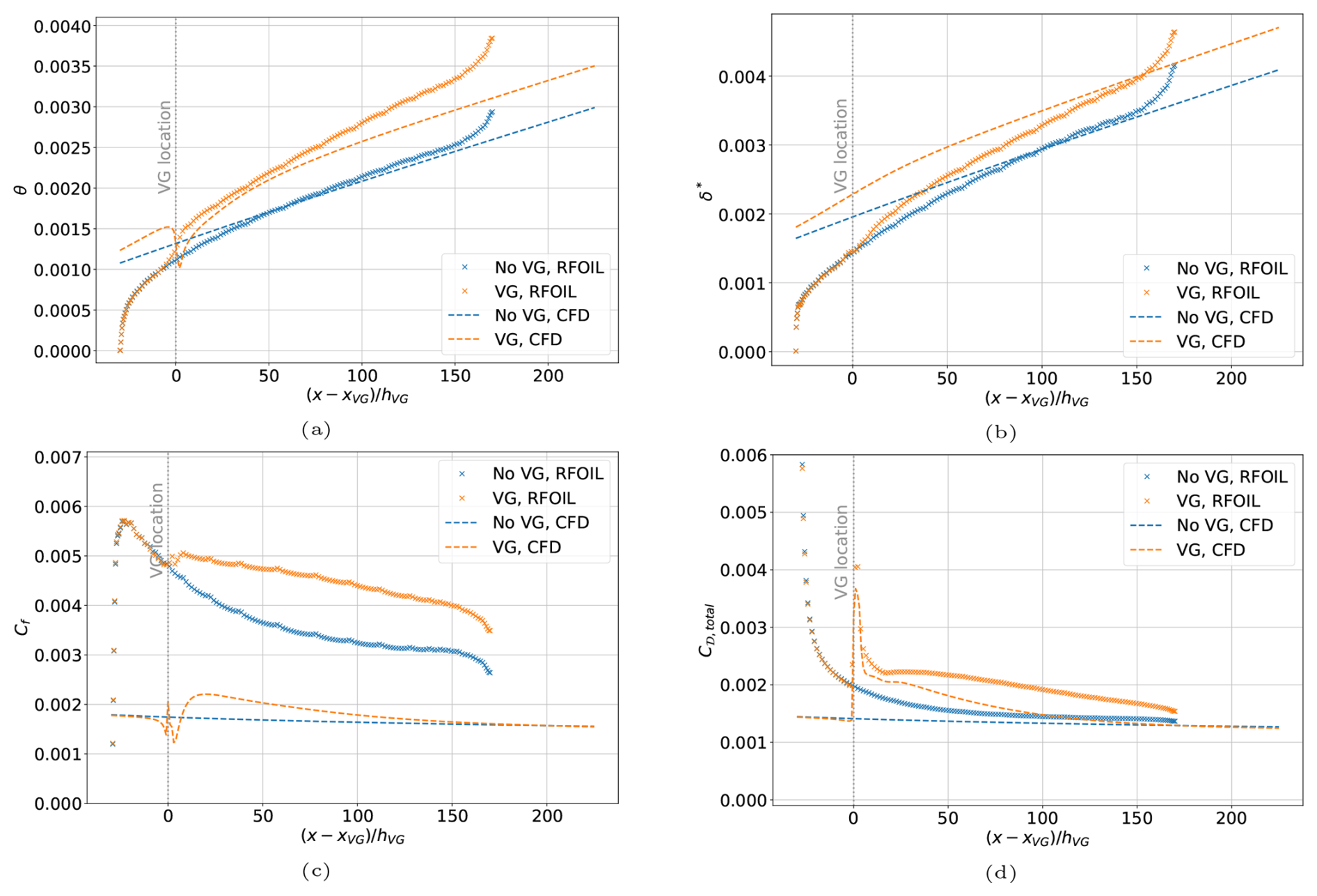
Figure 12 Verifying the VG model implementation in RFOIL by comparing the (a) momentum thickness, (b) displacement thickness, (c) skin friction coefficient, and (d) total viscous dissipation coefficient from the approximated turbulent flat plate in RFOIL to the flat-plate CFD calculations.

7 Validation of the new VG model in RFOIL

The proposed VG model is validated against wind tunnel lift polars for airfoils, focusing on the changes in positive stall angle and maximum lift between the no-VG and VG conditions. The validation database, summarised in Sect. A, consists of thicker airfoils (greater than 21 % thickness-to-chord ratio) tested at chordwise Reynolds numbers above 1 million, with and without VGs, in natural and forced transition conditions. In all comparisons, the new VG model is also compared to the current state-of-the-art models of XFOILVG and RFOILVG. The present VG model is denoted as “RFOILVogue” in all subsequent comparisons.

The experimental database used in the benchmark is split into two categories – data used to tune XFOILVG and RFOILVG and data outside the tuning dataset. The VG model implemented in XFOILVG and RFOILVG uses the lift polars of the airfoils and VGs in the tuning dataset to correct the lift slope of the no-VG polar to the target VG polar. Thus, the subsequent benchmark is presented in two parts. Section 7.1 and 7.3 show the evaluation of RFOILVogue's performance for the FFA-W3-241 and FFA-W3-301 airfoils with VGs. These airfoils were not used to develop XFOILVG/RFOILVG's tuned VG model. Thus, it highlights the accuracy and robustness improvements offered by RFOILVogue's analytical VG model for any general airfoil and VG configuration. We also discuss RFOILVogue's performance for a DU-97-W-300 airfoil, which is from XFOILVG/RFOILVG's tuning dataset in Sect. 7.2, to compare the analytical VG model to the engineering tuning approach.

7.1 Comparison for the FFA-W3-241 airfoil

The first benchmark case chosen for comparison is the flow over an FFA-W3-241 airfoil with a maximum thickness-to-chord ratio of 24.1 %. The airfoil features in the new IEA Wind 22 MW offshore reference turbine (Zahle et al., 2024) and is thus considered representative of a typical modern wind turbine rotor blade section. Moreover, this airfoil was not used to tune the VG model implemented in XFOILVG and RFOILVG, which makes it a perfect test case to compare the effectiveness of the older tuned VG models to the improvements produced by the proposed model. The wind tunnel data (Fuglsang et al., 1998) come from the tests performed by RISO in the VELUX wind tunnel in Denmark. The model chord is 0.6 m, and the chordwise Reynolds number is 1.6 million. The tests are performed in free and forced transition to simulate leading-edge erosion effects, as well as with and without VGs. Transition to turbulence is forced using a zigzag trip tape of 0.35 mm thickness. The trip tape was mounted at $x/c=\mathrm{0.05}$ on the suction side and $x/c=\mathrm{0.10}$ on the pressure side. The reported turbulence level corresponded to N=2.622 for the e^N transition check for the free transition calculations. Pressure distribution data are digitised from Fuglsang et al. (1998) for a select representative angle of attack included in the report to validate the flow around the airfoil from RFOIL calculations. While the exact values may have some digitisation errors, the overall trends and flow features from the pressure distribution data are still valid for comparison.

First, the performance of base RFOIL and XFOIL without VGs is compared to the wind tunnel data. It can be seen in Fig. 13 that RFOIL overpredicts the positive stall angle of attack by about 1° for the free transition case and by about 2° for the forced transition case. The slope of the lift polar in RFOIL is also higher, resulting in an overprediction of the maximum positive lift. From the chordwise pressure distributions for the free and forced transition cases without VGs in Figs. 15 and 17, it can be seen that RFOIL predicts a larger suction peak than the experiments, which leads to the overprediction of lift both in the linear part and near stall in the lift polar. At higher angles of attack, RFOIL also predicts the flow separation location to be further downstream than the experiments, explaining the delayed stall. The suction peak overprediction increases with angle of attack. It is also higher for forced transition cases than for free transition cases. The flow separation location is also further downstream than the experiment value in forced transition (a difference of about 10 % chord) compared to free transition (a difference of about 5 % chord).

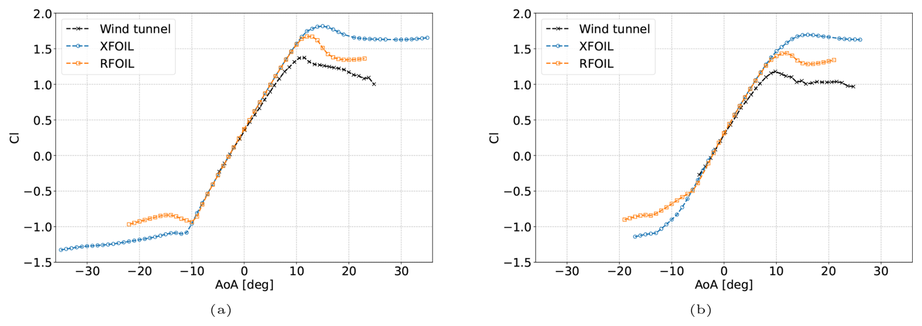
Figure 13 Establishing a baseline for RFOIL and XFOIL by comparing the lift characteristics of the FFA-W3-241 airfoil without VGs at 1.6 million Reynolds number in (a) free transition and (b) forced transition. Wind tunnel data taken from Fuglsang et al. (1998).

The VG cases consist of triangular vane VGs placed in a counter-rotating array on the upper side of the airfoil with the following geometry parameters:

• h=4, l=12, D=28, d=20 mm, and β=19.5°, denoted henceforth as the “4 mm VGs”,

• h=6, l=18, D=35, d=25 mm, and β=19.5°, denoted henceforth as the “6 mm VGs”.

When comparing the results for the VG cases in Figs. 14 and 16, the higher lift polar slope compared to wind tunnel measurements can be seen for both the previous VG models (XFOILVG and RFOILVG) and the current VG model (RFOILVogue). RFOILVG and RFOILVogue predict the same lift polar slope in the linear region. However, RFOILVogue better captures the stall onset for both the stall angle of attack and the maximum lift. The improvements are higher for the 4 mm VGs than the 6 mm VGs, with about 26 % improvement in capturing the maximum lift at stall for the 4 mm VGs compared to about 15 % improvement for the 6 mm VGs. Comparing the chordwise pressure distributions for free and forced transition cases with VGs in Figs. 15 and 17 reveals that RFOILVogue predicts a lower suction peak than RFOILVG, which is closer to the experiments, leading to a lift prediction closer to the experiment values. RFOILVogue also predicts an earlier flow separation point than RFOILVG, which explains the reason for a positive stall angle of attack closer to the experiment values. Additionally, these pressure distribution comparisons demonstrate that the new RFOILVogue model is able to accurately predict the flow around the airfoil at various adverse pressure gradients at various angles of attack. Moreover, the combination of the new VG model and the existing flow separation check method in RFOIL (as described in Sect. 5.5) enables prediction of the flow separation location around the airfoil to a similar degree of accuracy as the no-VG cases, which is crucial for accurate stall angle predictions.

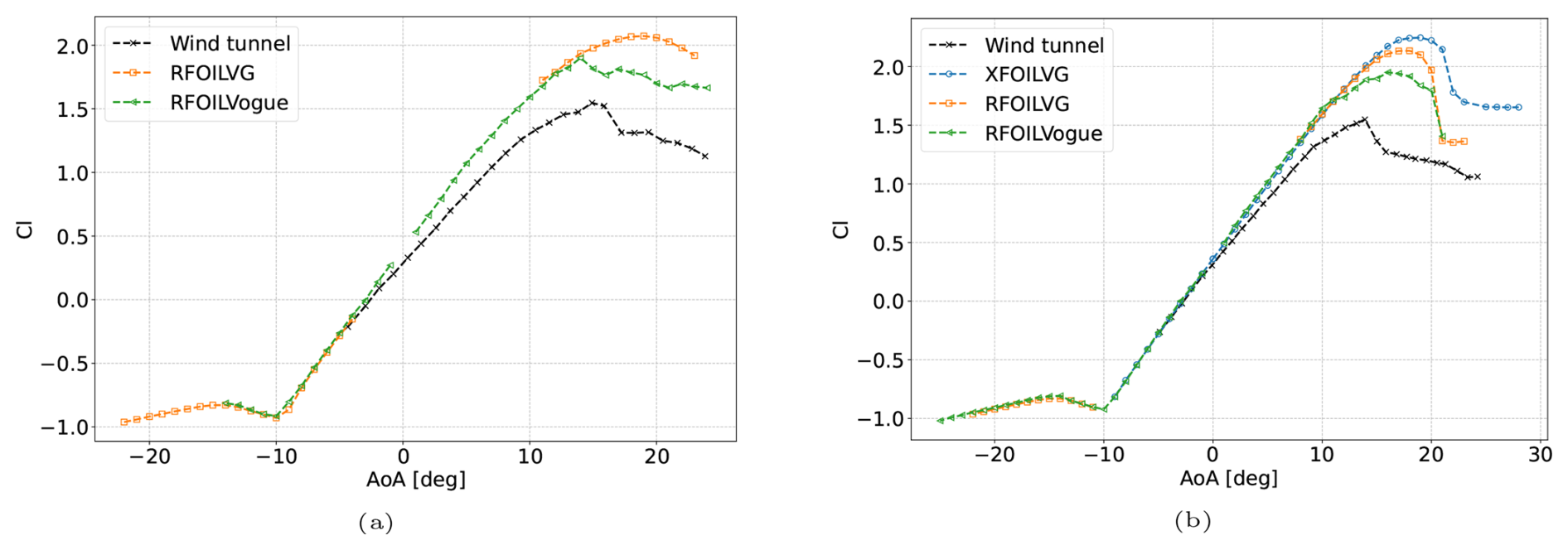
Figure 14 FFA-W3-241 airfoil in free transition with (a) 4 mm VGs placed at 20 % chord and (b) 6 mm VGs placed at 30 % chord on the upper side at a Reynolds number of 1.6 million. Wind tunnel data taken from Fuglsang et al. (1998).

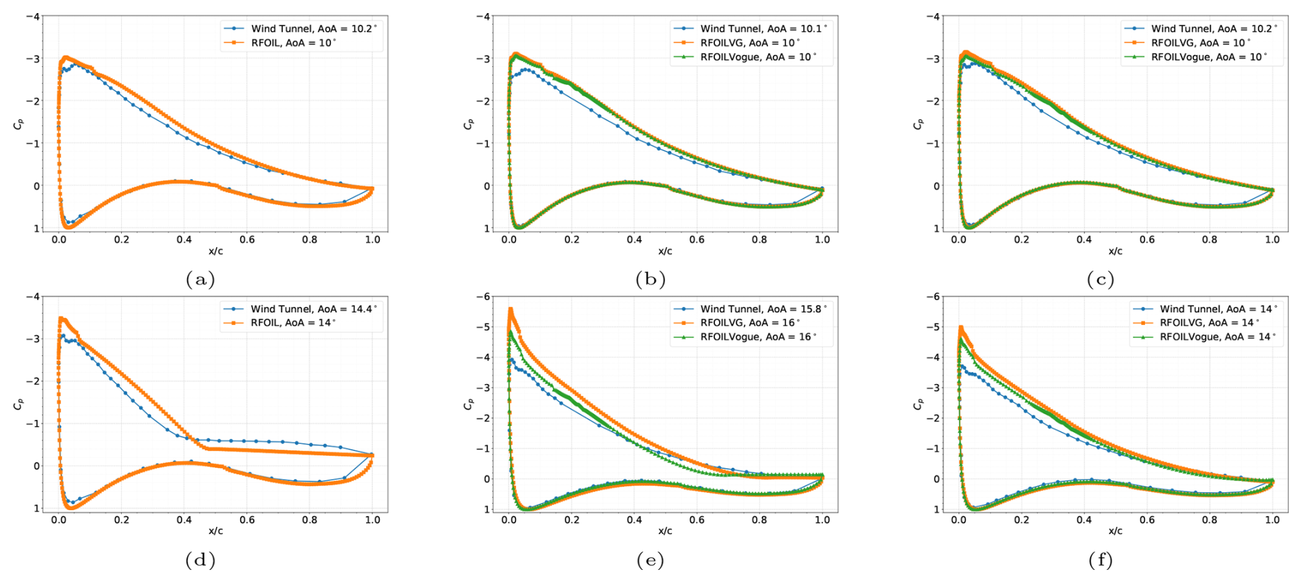
Figure 15 Chordwise pressure distributions at AoA 10° (top row) and AoA 14° (bottom row) with adverse pressure gradients for the FFA-W3-241 airfoil in free transition at a Reynolds number of 1.6 million with no VGs (a, d), 4 mm VGs placed at 20 % chord (b, e), and 6 mm VGs placed at 30 % chord (c, f) placed on the upper surface. Wind tunnel C_p data are digitised from Fuglsang et al. (1998).

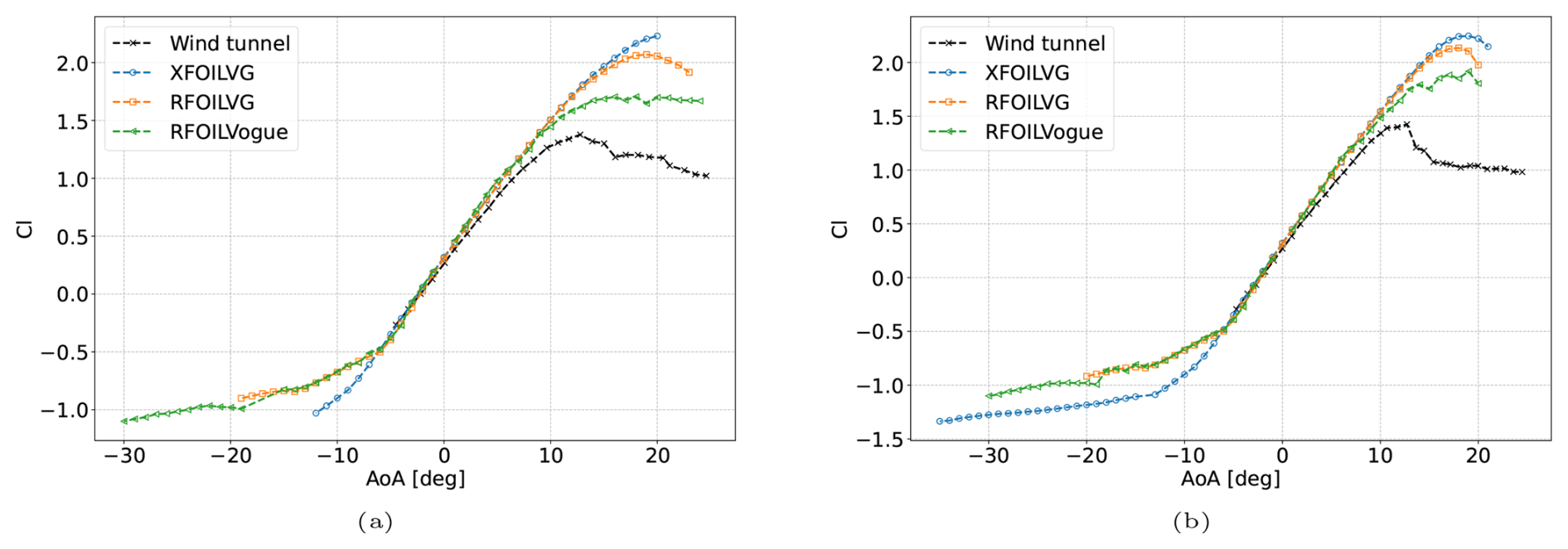
Figure 16 FFA-W3-241 airfoil with forced transition through zigzag tape with (a) 4 mm VGs placed at 20 % chord and (b) 6 mm VGs placed at 30 % chord on the upper side at a Reynolds number of 1.6 million. Wind tunnel data taken from Fuglsang et al. (1998).

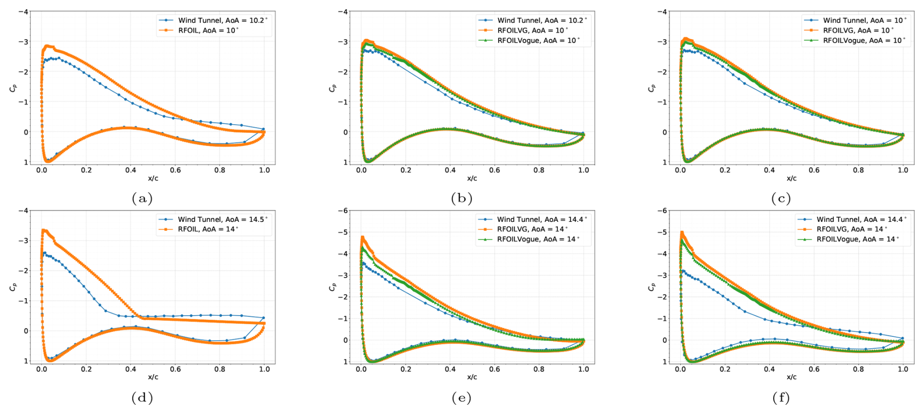
Figure 17 Chordwise pressure distributions at AoA 10° (top row) and AoA 14° (bottom row) with adverse pressure gradients for the FFA-W3-241 airfoil with forced transition using ZZ tape at a Reynolds number of 1.6 million with no VGs (a, d), 4 mm VGs placed at 20 % chord (b, e), and 6 mm VGs placed at 30 % chord (c, f) placed on the upper surface. Wind tunnel C_p data are digitised from Fuglsang et al. (1998).

RFOILVogue's predictions of stall margin variation with VG geometry parameters are also compared with the wind tunnel data. The vane size comparison between the larger 6 mm VGs and the smaller 4 mm VGs is shown in Fig. 18. The comparison of VG locations is shown in Fig. 19. Since drag data were unavailable for the experiments, the comparison between VG and no-VG RFOIL drag values is included only to compare expected trends.

RFOILVogue correctly predicts that the 6 mm VGs are more effective at delaying stall than the 4 mm VGs in free transition conditions in Fig. 18a. Larger VGs are also known from the literature (Baldacchino et al., 2018) to produce more drag because they cause a larger obstruction to the incoming flow. This trend is also captured in the drag plot in Fig. 18b.

RFOILVogue also correctly predicts in Fig. 19a that placing VGs further upstream at 20 % chord is more beneficial for stall delay than putting them at 30 % chord for this airfoil at the tested Reynolds number under free transition conditions. Placing VGs further downstream is expected to reduce the drag (Baldacchino et al., 2018) because a smaller portion of the airfoil boundary layer experiences the VG mixing that increases skin friction. This trend is also observed in the drag plot in Fig. 19b.

Overall, despite the overprediction in maximum lift in some cases, the new model predicts the correct parametric trends for variation in VG geometry and placement, which shows the tool's utility for design optimisation studies.

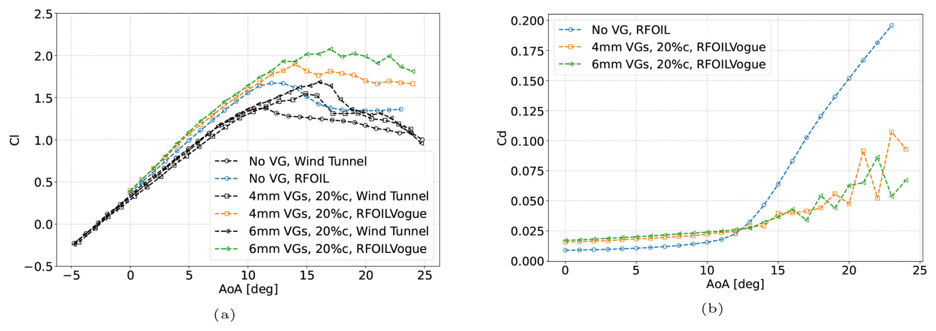
Figure 18 RFOILVogue (a) lift polars and (b) drag polars for various VG sizes placed at the same chordwise location showing that RFOILVogue predicts the expected maximum lift, stall delay, and drag trends when comparing VG vane sizes under free transition conditions. Wind tunnel data taken from Fuglsang et al. (1998).

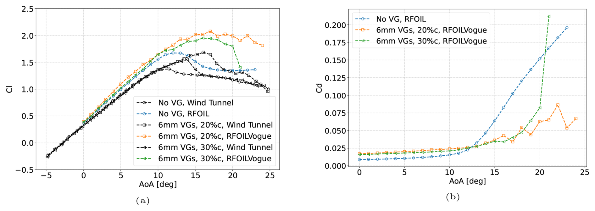
Figure 19 RFOILVogue (a) lift polars and (b) drag polars for the 6 mm VGs placed at different chordwise locations showing that RFOILVogue predicts the expected maximum lift, stall delay, and drag trends when comparing the chordwise placement location of VGs under free transition conditions. Wind tunnel data taken from Fuglsang et al. (1998).

7.2 Comparison for the DU-97-W-300 airfoil

The DU-97-W-300 airfoil was developed as a dedicated airfoil for wind turbine rotor blades (Timmer and van Rooij, 2003) and used in the AVATAR reference wind turbine (Schepers et al., 2015). It has a maximum thickness-to-chord ratio of 30 %. The wind tunnel data for this airfoil (Baldacchino et al., 2018) were acquired in the TU Delft Low-Turbulence Tunnel and is part of the tuning database for XFOILVG and RFOILVG. The model chord is 0.65 m, and the chordwise Reynolds number is 2 million. The selected test case consists of both free transition and forced transition measurements, with transition forced through a zigzag tape of height 0.35 mm at $x/c=\mathrm{0.05}$ on the upper side. The reported wind tunnel turbulence level corresponds to N=9 for the e^N transition check in the free transition calculations. Similar to the FFA-W3-241 case, the comparison for the no-VG case in Fig. 20 shows that RFOIL slightly overpredicts the lift slope polar and maximum lift. However, the free transition prediction is much closer to wind tunnel data for the DU-97-W-300 airfoil than the FFA-W3-241 airfoil. The pressure distributions for the free transition case without VGs are presented in Fig. 22 and for the forced transition case without VGs in Fig. 23 at different angles of attack indicating different adverse pressure gradients. RFOIL predicts the suction peak well when flow over the airfoil is attached and when flow is separated over a large part over the airfoil. The suction peak is overpredicted at medium angles of attack. The flow separation location is also predicted more downstream than the experiment data, around 10 % chord more downstream in both free and forced transition. The suction peak overprediction is lower than in the FFA-W3-241 case, which explains the better lift polar prediction. Similar to the FFA-W3-241 case, the suction peak overprediction is higher for forced transition than for free transition cases.

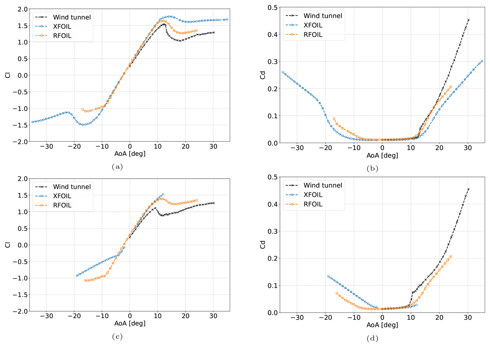
Figure 20 Establishing a baseline for RFOIL and XFOIL for the DU-97-W-300 airfoil at a Reynolds number of 2 million in (a)–(b) free transition and (c)–(d) forced transition with ZZ tape by comparing the lift and drag characteristics. Wind tunnel data taken from Baldacchino et al. (2018).

The VG case selected for comparison in this section uses triangular vane VGs placed in a counter-rotating array with the geometry parameters h=5, l=15, D=35, d=17.5 mm, and β=15° on the upper side. Compared to the experimental data, RFOILVogue performs at par with RFOILVG for the lift and drag in the linear region and the stall angle (Fig. 21). RFOILVogue overpredicts the maximum lift and the post-stall drag compared to RFOILVG. Thus, the present analytical VG model that models the integral boundary layer quantities can predict the lift polar to a similar degree of accuracy as the former tuned engineering model that corrects the lift polar for VG effects. The pressure distributions for the free transition case with VGs are presented in Fig. 22 and for the forced transition case with VGs in Fig. 23 at different angles of attack representing adverse pressure gradients of different strengths. Similar to the FFA-W3-241 airfoil, RFOILVogue predicts a lower suction peak than RFOILVG, although both VG models are now very close to the experiment values. Similarly, the flow separation location is predicted slightly more accurately by RFOILVogue than RFOILVG, but both VG models are close to experiment values. The fact that the old RFOILVG is tuned on the experiment data for this airfoil is visible in the relatively small differences between the VG models. Nevertheless, these pressure distribution comparisons further demonstrate the capabilities of the new RFOILVogue model to accurately predict the flow around the airfoil, including the flow separation location, under strong adverse pressure gradients at various angles of attack.

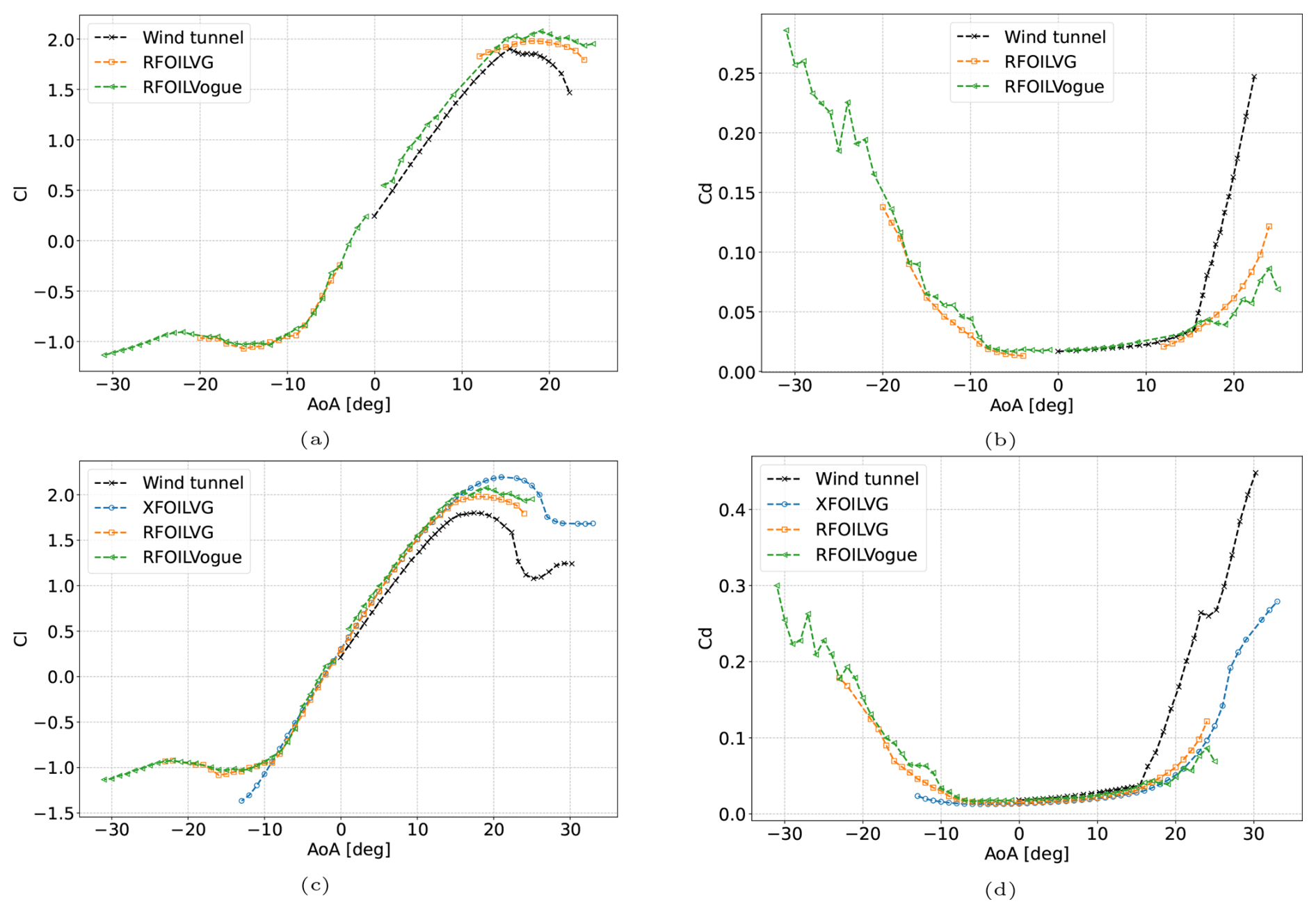
Figure 21 RFOILVogue predicts the same stall angle and slightly worse maximum lift than RFOILVG for the DU-97-W-300 airfoil with 5 mm VGs placed at 20 % chord on the upper side at a Reynolds number of 2 million in (a) free transition and (b) forced transition through zigzag tape. Wind tunnel data taken from Baldacchino et al. (2018).

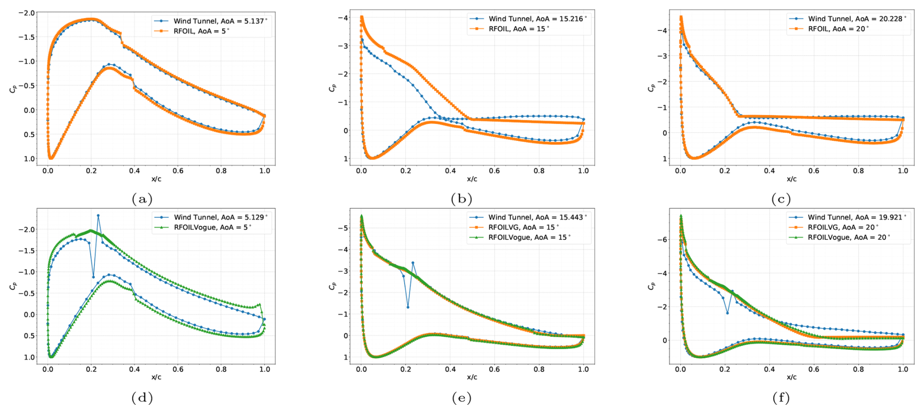
Figure 22 Chordwise pressure distributions at AoA (a, d) 5°, (b, e) 15°, and (c, f) 20° with adverse pressure gradients for the DU-97-W-300 airfoil in free transition at a Reynolds number of 2 million. The top row is without VGs, and the bottom row is with 5 mm VGs placed at 20 % chord on the upper side. The previously proposed RFOILVG model does not converge at 5° angle of attack. Wind tunnel data taken from Baldacchino et al. (2018).

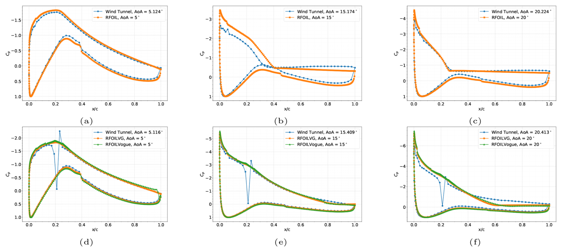
Figure 23 Chordwise pressure distributions at AoA (a, d) 5°, (b, e) 15°, and (c, f) 20° with adverse pressure gradients for the DU-97-W-300 airfoil with forced transition using ZZ tape at a Reynolds number of 2 million. The top row is without VGs, and the bottom row is with 5 mm VGs placed at 20 % chord on the upper side. Wind tunnel data taken from Baldacchino et al. (2018).

The new model outperforms the older tuned models when predicting the actual boundary layer properties. The displacement and momentum thicknesses from the boundary layer are compared between RFOILVogue, RFOILVG, and fully turbulent RANS CFD calculations of this airfoil and VGs in Fig. 24. We select the case of 8° angle of attack, where there is a strong pressure gradient, but the flow is still attached. This allows for comparing the model predictions for an adverse pressure gradient case to the zero-pressure gradient flat plate.

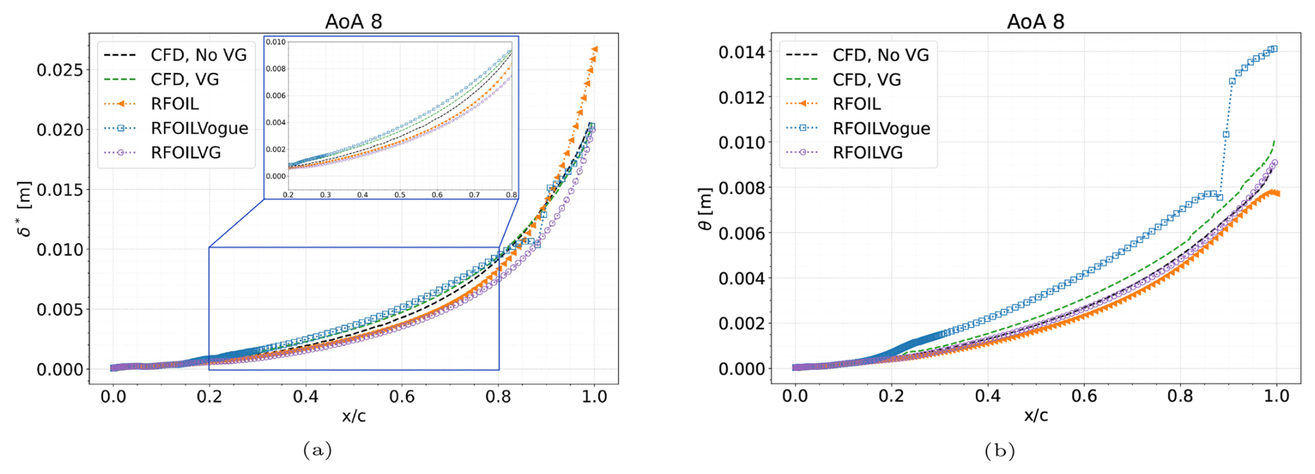
Figure 24 Comparing the (a) displacement thickness and (b) momentum thicknesses predicted by RFOILVG and RFOILVogue for the DU-97-W-300 airfoil with forced transition through zigzag tape and 5 mm VGs placed at 20 % chord on the upper side at 8° angle of attack at a Reynolds number of 2 million.

The new RFOILVogue predicts a nearly identical value to CFD calculations for the displacement thickness at 8° angle of attack, except for a small part of the airfoil near the trailing edge. RFOILVG underpredicts the displacement thickness for the same case. RFOILVogue overpredicts the momentum thickness compared to CFD results, while RFOILVG underpredicts the momentum thickness. These results contrast with the simulated flat-plate case in Sect. 6. In the flat-plate comparison, the VG model underpredicted the displacement thickness near the VG location and overpredicted the momentum thickness far from the VG location, resulting in a net lower shape factor and higher mixing. For the airfoil case, the VG model still predicts higher mixing but this time mainly because of a higher momentum thickness estimation. Thus, for the adverse pressure gradient airfoil case, the VG model predicts the mass transfer well but predicts a much higher momentum in the boundary layer than expected from CFD.

7.3 Comparison for the FFA-W3-301 airfoil

The FFA-W3-301 airfoil was developed as a thick airfoil for wind turbine rotor blades (Björck, 1990) with a maximum thickness-to-chord ratio of 30 %. It has been used in the design of the IEA 15 MW and 22 MW reference wind turbines (Gaertner et al., 2020; Zahle et al., 2024). The wind tunnel data for this airfoil with VGs were acquired in the Stuttgart Laminar Wind Tunnel and digitised from the work of Sorensen et al. (2014). The chordwise Reynolds number is 3 million. The data consist of the airfoil with and without VGs in free transition only. The reported turbulence level of the Stuttgart Laminar Wind Tunnel at this Reynolds number corresponds to N=9 for the e^N transition check in the free transition calculations of RFOIL. The comparison for the no-VG case in Fig. 25a shows that RFOIL only slightly overpredicts the positive stall angle of attack by about 1° and the maximum lift by about 5 % compared to the wind tunnel data. The VG case chosen for comparison consists of triangular vane VGs with vane array geometry parameters $h/c=\mathrm{0.01}$, $l/c=\mathrm{0.038}$, $d/c=\mathrm{0.06}$, $D/c=\mathrm{0.09}$, and β=15.5°. The VGs are placed on the suction side of the airfoil at 30 % chord. In the comparison between the VG models shown in Fig. 25b, RFOILVogue only overpredicts the positive stall angle of attack by about 1.5° and predicts the same maximum lift as the wind tunnel data. This is a significant improvement over RFOILVG, which overpredicts the stall angle of attack by about 4° and the maximum lift by about 7 %. Moreover, in the linear region, RFOILVG only converges from 6° angle of attack onwards, while RFOILVogue converges for all the tested angles of attack. This indicates an improvement in robustness of the new RFOILVogue model compared to the older RFOILVG. This can be attributed to fixing the transition point more accurately and modelling the upstream effects of the VGs in RFOILVogue, incorporating the influence of VGs on the boundary layer development.

Figure 25 Lift characteristics for the FFA-W3-301 airfoil in free transition (a) without VGs and (b) with VGs placed at 30 % chord. Height of the VGs is 1 % of the chord length. Wind tunnel data digitised from Sorensen et al. (2014).

8 Global performance assessment

Besides the selected cases discussed in Sect. 7, the performance of RFOILVogue and RFOILVG was compared for a broader database of airfoils equipped with VGs. The database consists of both cases used to tune RFOILVG and cases that fall outside of the training dataset. The accuracy and performance of RFOILVogue, RFOILVG, and XFOILVG in predicting the stall characteristics compared to wind tunnel data are summarised in Tables 2–3. A distinction is made between the code performance for the wind tunnel datasets that were used to tune RFOILVG (Table 3) and the wind tunnel datasets that are outside the training dataset of RFOILVG. This was done to especially highlight the broad capabilities of the boundary layer vortex-dynamics-based RFOILVogue model that does not rely on any airfoil tuning data for the VG model.

Figure 26 Lift characteristics for the (a) FFA-W3-241 airfoil, free transition, and VGs of height 6 mm placed at $x/c=\mathrm{0.3}$, as well as the (b) FFA-W3-301 airfoil, free transition, and VGs of height $h_{VG}/c=\mathrm{0.01}$ placed at $x/c=\mathrm{0.3}$. RFOILVogue calculations converge for the full range of positive angles of attack, while RFOILVG calculations only converge AoA 8° onwards for the FFA-W3-241 airfoil, and AoA 6° onwards for the FFA-W3-301 airfoil. Wind tunnel data taken from Fuglsang et al. (1998); Sorensen et al. (2014).

8.1 Accuracy

The errors in stall characteristics are defined as in Eqs. (40)–(41). The standard deviation s of the errors for N test cases is defined as in Eq. (42). The subscript “WT” refers to wind tunnel data, and “code” refers to the corresponding values from XFOIL or RFOIL as applicable.

$$\begin{array}{}\text{(40)}& {\displaystyle }\text{Error in stall angle, }{\mathit{ϵ}}_{\mathit{\alpha }}={\mathit{\alpha }}_{\mathrm{code}}-{\mathit{\alpha }}_{\mathrm{WT}}\text{(41)}& {\displaystyle }\text{Error in maximum lift, }{\mathit{ϵ}}_{C_l}={\displaystyle \frac{{C_l}_{\mathrm{code}}-{C_l}_{\mathrm{WT}}}{{C_l}_{\mathrm{WT}}}}\text{(42)}& {\displaystyle }s=\sqrt{{\displaystyle \frac{\mathrm{1}}{N-\mathrm{1}}}\sum _{i=\mathrm{1}}^N{\left({\mathit{ϵ}}_i-\stackrel{\mathrm{‾}}{\mathit{ϵ}}\right)}^{\mathrm{2}}},\text{where}\stackrel{\mathrm{‾}}{\mathit{ϵ}}\text{is the mean}\end{array}$$

Table 2 Performance assessment of the VG models for cases outside the tuning dataset of XFOILVG and RFOILVG.

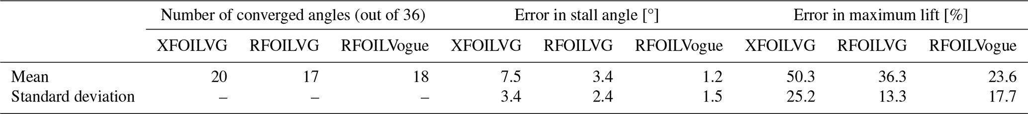
Table 3 Performance assessment of the VG models for the cases used to tune XFOILVG and RFOILVG.

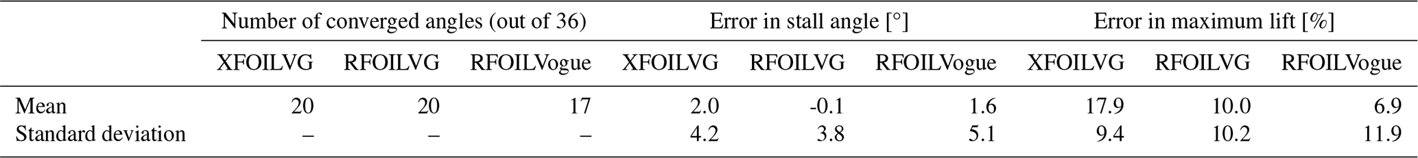
RFOILVogue is generally better than RFOILVG in the stall characteristics, predicting stall angles and maximum lift that are much closer to wind tunnel measurements. RFOILVogue captures the lift increase from the no-VG to the VG case more accurately than RFOILVG. For some cases that are used to tune RFOILVG, RFOILVogue only shows improvement compared to RFOILVG for the maximum lift predictions, while RFOILVG captures the stall angle better. In line with what is observed in earlier works for RFOIL and RFOILVG (Van Rooij, 1996; Sahoo et al., 2024), RFOILVogue also performs better than XFOILVG overall. This, however, is attributed to the improvements in base RFOIL over base XFOIL rather than the improvements in the VG model.

Besides the improvements in accuracy, the new RFOILVogue is also more robust, providing a converged solution for more angles of attack than RFOILVG. This was particularly true for free transition cases. This can be attributed to the new VG model's inclusion of the upstream effect of VGs on the boundary layer and its implementation of an earlier transition to turbulence upstream of the VG location, both missing in the VG model of RFOILVG. This is described in more detail in Sect. 8.2. RFOILVG converges for more angles for the airfoils included in its training dataset.

The starting point of this upstream effect is fixed at 10 heights upstream of the VG location based on observations from flat plates (as described in Sect. 5.4). However, the boundary layer comparisons between CFD and RFOIL calculations for the DU97W300 airfoil in Fig. 24 showed that the upstream effect starts closer to the VG location than 10 VG heights upstream. Capturing the upstream effect better can improve the robustness of the VG model even further. This is further elaborated on in Sect. 9 in the reflection on the impact of the VG model's inherent assumptions derived from flat-plate observations.

8.2 Robustness

The code robustness is compared by comparing the number of converged angles of attack in a polar calculation between 0 and 35°, increasing in increments of 1°. Besides the improvements in accuracy, the new RFOILVogue is also more robust, providing a converged solution for more angles of attack than RFOILVG. This was particularly true for free transition cases at angles of attack in the linear region, for instance the cases shown in Fig. 26. This robustness improvement for free transition cases is directly attributed to the new VG model's inclusion of the upstream effect of VGs on the boundary layer and its implementation of an earlier transition to turbulence upstream of the VG location, as described in Sect. 5.4, both of which are missing in the older RFOILVG. The effect of the difference in setting the forced transition location and including the upstream effect of VGs is only observed at low angles of attack, when the natural transition location is downstream or close to the VG location. At higher angles of attack, natural transition occurs far upstream of the VG location, and thus, the improved transition location fixing routine of RFOILVogue is never activated. Consequently, calculations from both VG models converge as usual.

9 Conclusions and future work

In this work, we used observations from flat-plate turbulent boundary layers under the effect of counter-rotating streamwise vortices to derive new spanwise-averaged integral boundary layer equations valid for incompressible turbulent boundary layers influenced by the presence of vortex generators. The exact derivation of the IBL equations without significant assumptions ensured that the IBL framework for VGs derived in this work can be used for flat plates and airfoils alike. To model the new IBL framework in an airfoil analysis tool like RFOIL, which uses a viscous–inviscid interaction method to solve for the flow around the airfoil, we first identified the most significantly changed terms in the IBL framework for VGs to be the shape factor and the viscous dissipation. We then proposed a model that connects the changes in the boundary layer quantities to the vortex generator array geometry parameters and the flow Reynolds number. Implementing this model in RFOIL, we created an extended version named RFOILVogue that can analyse a broad range of airfoils and vortex generator configurations to calculate aerodynamic forces. A benchmark of RFOILVogue and the older RFOILVG against wind tunnel measurements of airfoils with VGs showed that RFOILVogue performs better than older models like RFOILVG when it comes to positive stall angle and maximum lift predictions. Comparisons of the pressure distribution (where available) and integral boundary layer quantities with CFD calculations showed that the inclusion of vortex dynamics in the IBL equations imparts RFOILVogue with the ability to predict boundary layer properties, such as the strength of the suction peak, the flow separation point, and the momentum thickness, more accurately than RFOILVG. Besides accuracy improvements, the new RFOILVogue is also more robust than RFOILVG, particularly for free transition cases, due to improvements in the RFOILVogue code allowing for better convergence. Overall, RFOILVogue is more generalised than RFOILVG, capable of modelling various families of airfoils and vortex generators. The paper also provides a methodology to formulate the integral boundary layer equations for VGs from flat-plate boundary layer observations. This methodology can serve as a basis to formulate reduced-order boundary layer models for other airfoil add-ons that modify the boundary layer over the airfoil surface and integrate the developed reduced-order boundary layer frameworks into tools like RFOIL. While RFOILVogue is an improvement over RFOILVG, it still suffers from the inherent limitations of reduced-order methods like the viscous–inviscid interaction method that RFOIL itself is based on. In some cases, the maximum lift can be overpredicted by as much as 23 %, which still leaves much to be desired for the accuracy of RFOIL and any VG models implemented in it. Generally, this discrepancy between RFOILVogue and experiments is more pronounced for thicker airfoils, which are more challenging to model in RFOIL even without VGs. However, limited wind tunnel data for thick airfoils were available to the authors, and the VG model must be benchmarked against more wind tunnel datasets for thick airfoils to shed light on the underlying reasons behind the drawbacks of RFOIL and RFOILVogue for thick airfoils. Another area of improvement for the model is the refinement of the upstream effects of VGs and transition to turbulence induced by different VG configurations for adverse pressure gradients. The turbulence shear lag equation encapsulates these effects, and the relationship between the turbulent shear stress and the boundary layer quantities is mainly contained in the G−β relationship between the scaled pressure gradient and shape factor. Investigating these will enhance accuracy in the free transition cases by predicting the impact of VGs on natural transition more accurately. Overall, the new RFOILVogue is a demonstration of a VG model that incorporates the effects of vortex dynamics on turbulent boundary layers to formulate a reduced-order boundary layer model. This model is more robust and generalised than the earlier tuned models from the literature and is capable of modelling various families of airfoils and vortex generators. Besides the improvements in accuracy and robustness, the VG model derived from boundary layer observations also provides a methodology to develop reduced-order models for VGs and other airfoil add-ons without dependence on expensive wind tunnel measurements of an extensive range of airfoils.

Appendix A: Datasets for model benchmark

Timmer and van Rooij (2003)Timmer and van Rooij (2003)Baldacchino et al. (2018)Fuglsang et al. (1998)Sorensen et al. (2014)Sorensen et al. (2014)

Table A1 Summary of reference data.