Evaluation of a high-resolution regional climate simulation for surface and hub-height wind climatology over North America

Assessing the availability of key wind resources requires augmenting observations to support the implementation of wind energy infrastructure. However, observations are limited, necessitating the development of high-resolution, long-term gridded datasets. This study presents a robust, dynamically downscaled climatological dataset, offering 20 years of hourly wind data at a 4 km spatial resolution across North America, and evaluates its performance against observations, including meteorological towers and automated surface-observing system (ASOS) stations, as well as coarse-resolution reanalysis data (the European Centre for Medium-Range Weather Forecasts (ECMWF) reanalysis version 5 (ERA5)). Results demonstrate that the downscaled high-resolution wind data outperform ERA5 in regions of complex terrain and coastal areas, with improved overlap coefficients for wind data distributions and reduced root mean square errors (RMSEs) for hub-height and near-surface diurnal wind patterns. The downscaled simulation also captures the synoptic drivers of seasonal wind direction patterns reasonably well, indicated by high wind rose similarity indices. This study also provides an analysis of interannual variability, utilizing the dataset's full 20-year period, and model uncertainty, generated by varying model initial conditions and physics parameterizations across 1-year ensemble members, which are key considerations for wind resource assessment in wind farm development.

1 Introduction

Wind is a key factor in shaping a region's complex climate, influencing both environmental and economic sectors. Understanding local and regional wind variability is vital for assessing wind energy potential, which aids in the efficient implementation and operation of wind farms (Millstein et al., 2019; Couto and Estanquiero, 2022). Additionally, evaluating wind speed and direction is essential for conducting accurate climatological assessments to determine the long-term changes in regional wind patterns. However, the spatiotemporal coverage of current wind measurements remains very limited, particularly over complex terrains (e.g., western US), offshore, and at hub-heights, where wind energy resource assessments are crucial.

To bridge the gap between limited observational data and the need for accurate wind resource assessments, global and regional reanalysis datasets, such as Modern-Era Retrospective analysis for Research and Applications version 2 (MERRA-2), the North American Regional Reanalysis (NARR), and the European Centre for Medium-Range Weather Forecasts Reanalysis version 5 (ERA5), are commonly used (Hersbach et al., 2020; Gelaro et al., 2017; Mesinger et al., 2006). These reanalysis datasets provide valuable insights into wind patterns, variability, and long-term trends, and are also crucial for capturing climatological oscillations and large-scale circulations that influence wind characteristics (e.g., Sheridan et al., 2022a). While these datasets typically have higher horizontal resolution than global climate models (GCMs), they still lack the resolution necessary to explicitly resolve convection and represent fine-scale surface variations, which is essential for capturing convectively driven precipitation and wind (Murakami, 2014; Jones et al., 2021). Additionally, validating these reanalysis datasets is essential for determining their viability for wind resource assessments (Sheridan et al., 2020, 2025; Lee et al., 2014). For example, Sheridan et al. (2022b) found that ERA5 generally underestimates wind speed diurnal cycles based on 62 sites at a variety of heights above ground across the continental United States (CONUS). This underestimation is most prominent in late afternoon, caused primarily by the underestimation of convectively driven strong winds. Similarly, Chen at al. (2024) and Wilczak et al. (2024) found that ERA5 showed significant negative biases for wind speeds in areas of complex terrain, especially over the Rocky Mountains.

To achieve the necessary high resolution to capture finer-scale wind patterns over large spatial areas and extended time periods, researchers employ a technique called dynamical downscaling. This technique involves using initial and boundary conditions from the global or regional reanalysis data to force simulations at finer resolutions using a regional climate model. Regional climate modeling at a convection-permitting (CP) resolution, with a horizontal grid spacing of less than approximately 4 km, has become a promising approach for delivering more reliable climate information at regional and local levels. By directly resolving deep convective processes rather than relying on parameterization, these models demonstrate significant enhancements (e.g., Prein et al., 2015, and references therein). Due to recent breakthroughs in computational capacity and data management, several studies have been able to perform convection-permitting regional climate model (RCM) simulations. These simulations, especially those concentrating on CONUS (e.g., Draxl et al., 2015b; Gensini et al., 2022; Liu et al., 2017; Rasmussen et al., 2023), have shown substantial progress in depicting precipitation, wind, and high-impact weather from national to regional spatial scales. Among these, Draxl et al. (2015a, b) presented the largest freely available wind dataset at the time of its development, serving the Wind Integration National Dataset (WIND) Toolkit for wind resource assessment and grid integration studies. The data provide time series of meteorological variables every 5 min and 2 km across CONUS in the 7 years from 2007 to 2013.

This study builds upon previous efforts by presenting an additional high-resolution, long-term dataset, along with ensemble simulations for quantifying model uncertainty, for utilization in climatological wind assessments. The dataset was generated by a regional climate model using the Weather Research and Forecasting (WRF) model. With 4 km resolution, 20-year hourly output, and a model domain spanning the majority of North America and surrounding oceans, this dataset provides a spatiotemporal extension to existing climatological wind analyses. With large geographic coverage, this data product also offers insight into more remote, topographically complex regions, potentially highlighting viable areas for wind energy outside of CONUS. By leveraging a single large spatial domain, the model evolved as one system, developing its own natural variability without being constrained by the forcing data. This dataset has been leveraged by the latest WIND Toolkit Long-term Ensemble Dataset (WTK-LED), as documented by Draxl et al. (2024), serving as the WTK-LED Climate dataset (Table ES-1 in Draxl et al., 2024). Ultimately, this high-resolution dataset aims to combine the climatological significance of an extensive temporal length with the wind resource utility advantages of a large spatial domain.

Our study validates the dynamically downscaled model wind speeds and wind directions against various observational data at both the near-surface and turbine heights at mostly inland and onshore locations, investigating model performance at different temporal scales (diurnal, seasonal, interannual variability). In the context of wind energy in particular, both speed and direction are crucial components to consider when maximizing the efficacy and operability of wind farms, as speed largely determines the amount of power generated, while direction can incite microscale differences in wake effects. A complementary study evaluating the same dataset but focusing on CONUS coastal areas has been conducted by Sheridan et al. (2025). Our validation is also performed on the forcing data – ERA5 reanalysis (Hersbach et al., 2020) – aiming to understand the added value of the dynamically downscaled model to its coarser-resolution forcing data. Additionally, this study seeks to augment insights into model uncertainty within wind simulations that are brought about by varying model configurations.

This paper is organized in the following structure. The methodology (including model description), observational datasets used for validation, and analysis metrics used for evaluation are outlined in Sect. 2. The results of the model's performance at hub heights and near the surface are presented in Sect. 3.1 and 3.2, with an exploration of model bias in Sect. 3.3. Interannual variability and model uncertainty are quantified in Sect. 3.4 within the context of wind energy implications. Lastly, a summary of our findings and avenues for future research are discussed in Sect. 4.

2 Methods and datasets

2.1 Model setup

The wind validation performed in this study was based on a 20-year (2001–2020) climatological dataset produced by the WRF model (Powers et al., 2017) version 4.2.1 with the Advanced Research WRF dynamic core (Skamarock et al., 2008): the Argonne Downscaled Data Archive version 2 (ADDA v2). With a domain of 2050 × 1750 grid points at a 4 km grid spacing (8200 km × 7000 km), the model featured over 3.5 million grid cells, horizontally spanning the majority of North America and the Caribbean islands (Fig. 1a in Akinsanola et al., 2024). The model was run with 50 unevenly spaced sigma levels, 18 of which were within the lowest 1 km (8, 25, 42, 58, 75, 104, 147, 189, 231, 274, 317, 360, 403, 468, 555, 643, 777, and 957 m above ground level) and 10 of which were below 300 m above the ground, to ensure that the hub-height winds were calculated directly by the model. Initial and lateral boundary conditions were determined by ERA5. The model was reinitialized for each year on 1 November, ultimately producing a series of 20 simulations with a duration of 14 months each, covering the period from 2001–2020. The first 2 months (November and December) of each year were discarded as spinup time and not used for the data analysis. The reinitialization approach was chosen since the RCM was driven by high-resolution reanalysis data instead of coarse-resolution GCMs, which usually require at least 1 year of spinup time. While soil moisture is typically a concern when reinitializing models during the cold months, the soil moisture of both the ERA5 forcing data and ADDA v2 was validated and found to be realistic (Akinsanola et al., 2024).

Table 1 WRF model setup and ensemble runs used in ADDA v2 simulations.

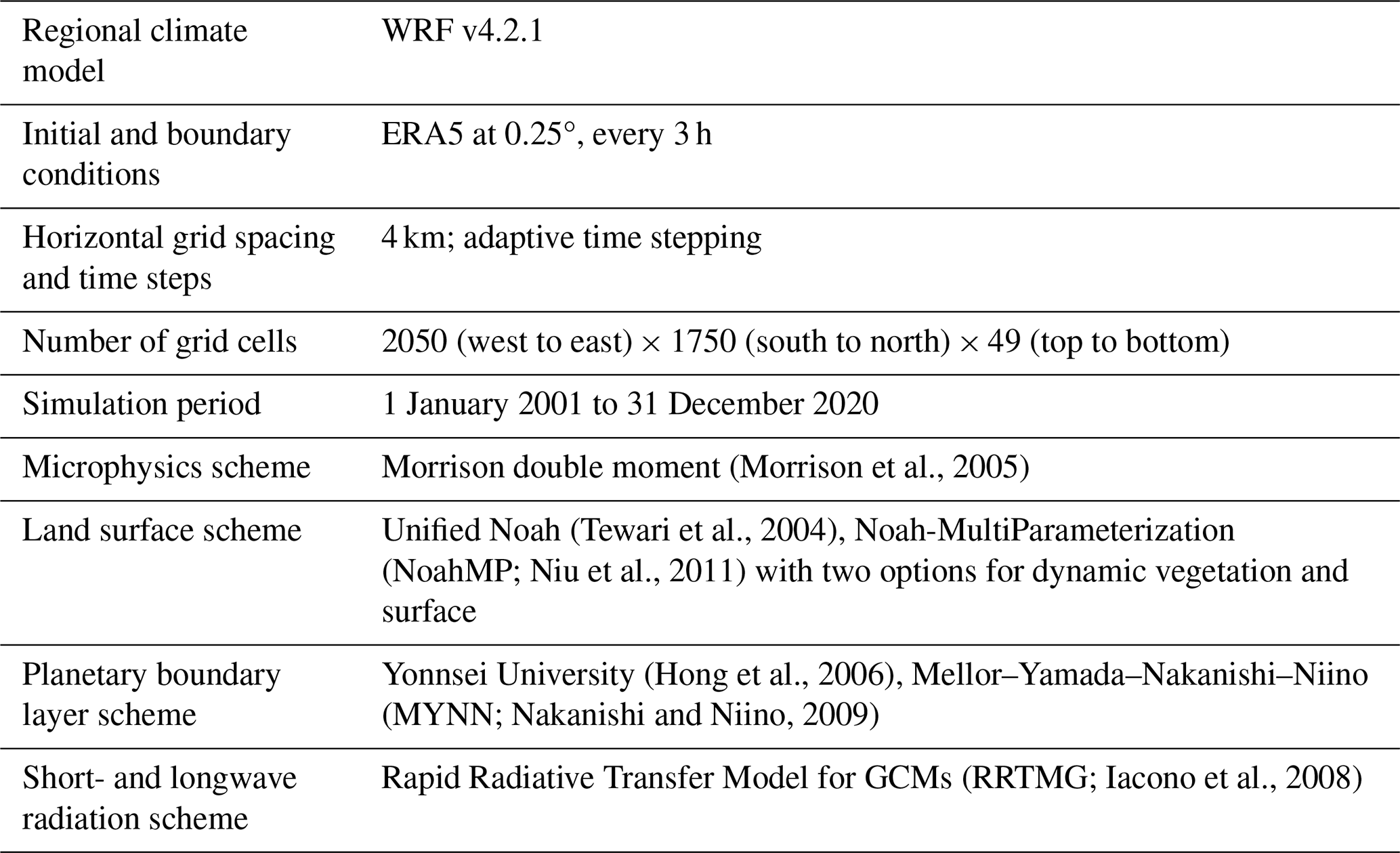
The Yonsei University (YSU) planetary boundary layer (PBL) scheme was used for these simulations, which runs with topographic correction for surface winds (topo_wind = 1 WRF; Jiménez and Dudhia, 2012; Skamarock et al., 2019) to represent extra drag from subgrid topography and enhanced flow at hilltops. The surface layer scheme used was the MM5 similarity scheme, which follows the Monin–Obukhov similarity theory (Monin and Obukhov, 1954) alongside the Carlson–Boland similarity functions (Carlson and Boland, 1978). The unified Noah land surface model was used for the land surface processes, which employs a four-layer soil temperature and moisture scheme, as well as fractional snow cover and frozen soil physics (Tewari et al., 2004). A full list of model parameterizations can be found in Table 1. No internal grid nudging or spectral nudging was employed for these simulations because it requires additional computational resources (20 %–30 % more for our configuration), and the ERA5 forcing data are at a relatively higher resolution than other reanalysis datasets, which can provide good boundary conditions and allow the model to develop its own spatiotemporal variability. Model output data for the most used meteorological variables, such as air temperature, wind speed and direction, and precipitation, were saved at hourly intervals for the full domain from 2001–2020. Other variables used less frequently were saved at 3 h intervals.

2.2 Model uncertainty

There are multiple sources of model uncertainty in regional weather and climate models (Hawkins and Sutton, 2009). The dominant uncertainty for near-term simulations includes model internal variability and structural uncertainty. Internal variability is caused by varying initial conditions, while structural uncertainty is generated by various physics parameterizations. To study the model's internal variability, we conducted 10 additional 1-year (El Niño–Southern Oscillation neutral year – 2018) ensemble runs, all with the same model setup as described in Sect. 2.1 but with different initial conditions (Wang et al., 2018). This was achieved by running each of the 10 ensemble members 12 h apart, with the first being initialized on 1 November 2017 at 00:00 UTC and the last being initialized on 5 November 2017 at 12:00 UTC. Thus, the slightly different initial conditions at each respective start time acted as the catalyst to generate differences between the ensemble members. The number of internal variability ensembles was chosen based on the logic of Wang et al. (2018), who demonstrated that 10 ensemble members with varying initialization times was the minimum number needed to capture the internal variability of the model.

To investigate the model's structural uncertainty arising from important physics parameterizations for wind, namely the PBL and land surface model (LSM), an additional six ensemble members were generated for the same neutral year 2018. Each ensemble member shared the same domain and spatial resolution but employed two different and widely used PBL schemes (YSU and MYNN) and LSMs (Noah and NoahMP) for wind energy applications (Draxl et al., 2014; Yang et al., 2017). The MYNN PBL scheme is a level 2.5 closure scheme for turbulence and implicitly solves for turbulence using parametric equations. It gives estimates of turbulent kinetic energy and dissipation rates within the boundary layer of the atmosphere (Nakanishi and Niino, 2009). NoahMP is an improved version of the Noah LSM and provides better representations of terrestrial biophysical and hydrological processes (Niu et al., 2011). A major physical mechanism enhancement includes improved treatment of soil moisture. Two dynamic vegetation options and two surface layer drag coefficient calculation options were also perturbed within the NoahMP LSM. Thus, in total we had 10 combinations, with 5 LSM options and 2 PBL options. We experimented with these 10 runs for a subregion over the Southern Great Plains (with various topographic characteristics) and determined that 6 of the 10 runs were able to capture the range of model uncertainty across the domain. Then, we used these six representative combinations for the entire North American domain and entire year of 2018. While the 16 ensemble members do not capture all model uncertainty, they do represent a robust range of model variability due to these perturbations in initial conditions and key physics parameterizations (see more details in Draxl et al., 2024).

2.3 Observational datasets used for validation

The validation performed on ADDA v2 used wind speed observational data taken within 100 m above ground level. The first collection of observations focused on hub-height wind speeds and wind directions. These observations were taken from multiple meteorological towers hosted by the US Department of Energy National Laboratories (Argonne National Laboratory, Brookhaven National Laboratory, NREL, Oak Ridge National Laboratory, Pacific Northwest National Laboratory, Savannah River National Laboratory) and the National Oceanic and Atmospheric Administration (National Centers for Environmental Information, National Data Buoy Center). In total, 26 meteorological towers were sampled and quality controlled for this analysis, with wind speed observations taken anywhere from 10 to 100 m above ground level. Observations were quality controlled through the process of removing atypical or unphysical reported wind speeds (less than 0 m s⁻¹, greater than 50 m s⁻¹, or non-varying values over periods of time greater than 3 h), based on Sheridan et al. (2025). Mast flow distortion corrections were not implemented since most locations had only one anemometer reading. For sites with multiple anemometer readings, instrumentation metadata, such as anemometer orientation with respect to nearby structures, were not included, and we did not want to make corrective assumptions. While different factors, such as instrument precision, environmental effects such as land use, obstructions, or elevation effects, and temporal sampling methods can introduce uncertainty into the collected observational wind, the quality control procedures conducted here maximize the integrity and reliability of the data used for this validation.

Table 2 Information of the hub-height wind data sourced from meteorological towers across CONUS. The number listed for each location corresponds to the numbers in Fig. 1, identifying the geographic positions of the meteorological towers. Location coordinates for proprietary data were excluded.

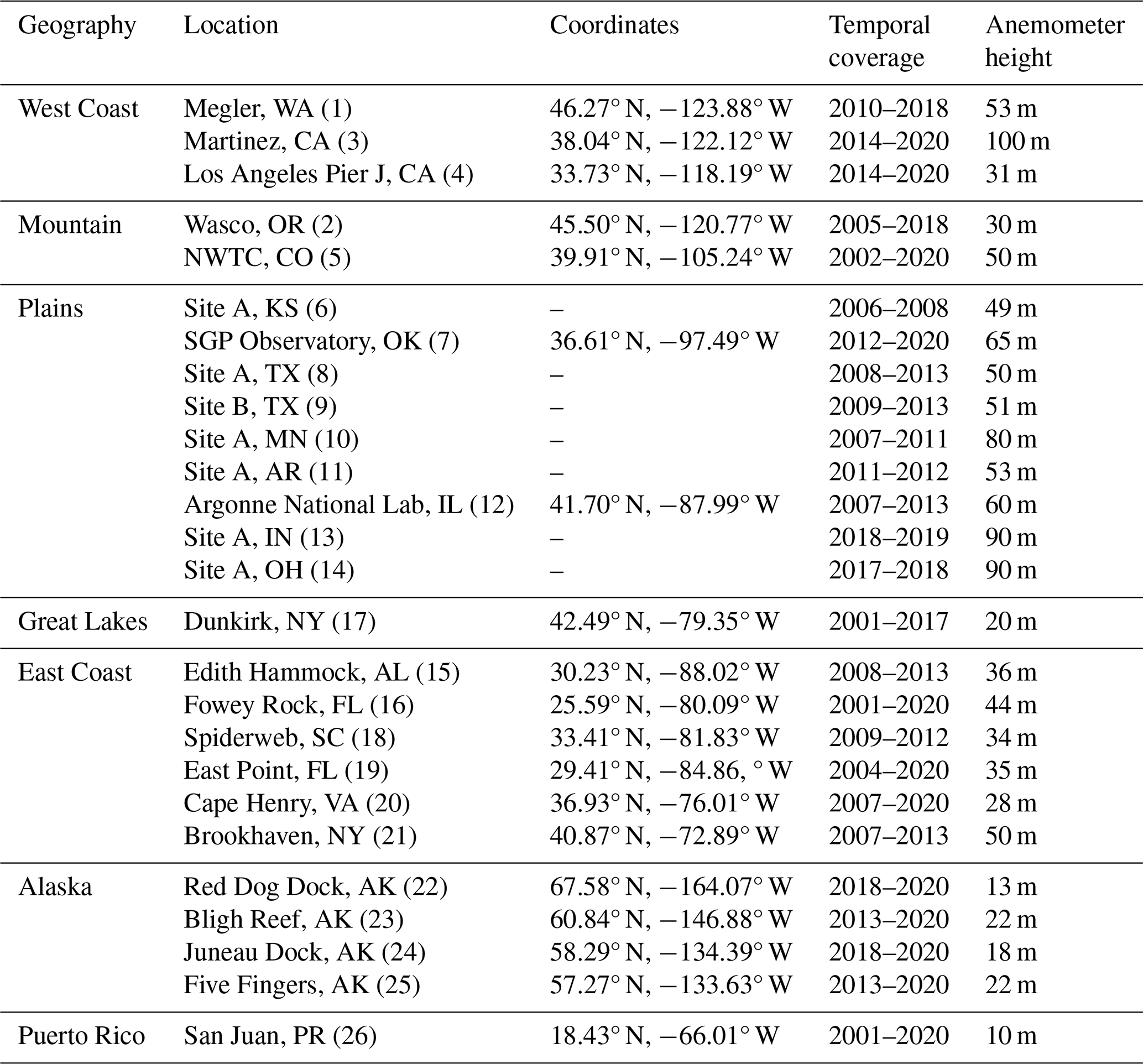
Temporal coverage for the meteorological towers varied between 2–20 years, with an average of ∼ 8.1 years. Observations covered a diverse range of geographies, including mountainous, coastal (East Coast and West Coast of CONUS), Great Lakes, and plain regions; Alaska and Puerto Rico (Caribbean) were denoted as separate geographic regions. For 19 of these meteorological towers, the exact locations, anemometer heights, and temporal coverages of wind observations can be found in Table 2. The remaining seven are proprietary data, for which exact locations could not be specified. While turbine-height wind speed and wind direction data are sparse, we have leveraged all publicly available resources that we have access to and performed a thorough validation over diverse geospatial areas.

The second part of this evaluation explores an expansive collection of 10 m wind speed data sourced from a network of automated surface-observing system (ASOS) stations. These stations monitor and report various meteorological variables and are operated by the United States National Weather Service, the Federal Aviation Administration, and the Department of Defense. The specific dataset used for this validation was collected from the Iowa Environmental Mesonet (IEM) and subsequently quality controlled by the Data Archive and Portal (DAP) platform. The dataset hosts over 2000 sites across CONUS and Alaska and covers a temporal period from 1 January 2000–31 December 2021, offering a spatiotemporally comprehensive means for performing a thorough validation of ADDA v2's 10 m wind. Additionally, wind speed data from four additional ASOS stations over Puerto Rico were downloaded from the IEM to spatially expand the model validation and gain a more comprehensive understanding of model performance over areas of sparse data availability and complex terrain.

To demonstrate the potential added value of ADDA v2 to its coarse-resolution forcing data, we also included ERA5 reanalysis in all near-surface and hub-height evaluations. ERA5 outputs only two levels of wind (10 and 100 m), so to evaluate winds at heights between these levels, an interpolation method was required. At each timestamp, the ADDA v2 and ERA5 wind speeds were adjusted to the observational heights via the power law using the model wind speeds at surrounding output heights to the observation height. While this interpolation method may induce some bias in both ADDA v2 and ERA5, the differences between these datasets are driven mostly by the difference in spatial resolution and the value added by ADDA v2. This approach was selected based on the analysis of Duplyakin et al. (2021), who found that the power law minimized errors due to vertical adjustment of wind dataset output heights to observation heights.

2.4 Statistics for validation

The wind speed validation in this study utilizes several statistical error metrics to evaluate how well ADDA v2 performs against observations. Root mean square error (RMSE), Pearson correlation coefficients (r), overlap coefficients (OVLs), and wind rose similarity indices (WRSIs) are used.

The RMSE gives a metric for the overall accuracy of the model, with lower RMSEs indicating improved model performance. RMSE is taken as the square root of the average of the squared differences between simulated wind speeds and observed wind speeds at various timescales (seasonal, monthly, diurnal), given by Eq. (1). This metric is effective at highlighting instances of larger errors in the model and demonstrates the overall magnitude of model inaccuracy. Here, n represents the number of wind speed observations (in time), v_mod represents the modeled wind speed, and v_obs denotes the observed wind speed. Relative RMSE (rRMSE) was also considered (Eq. 2) by dividing the RMSE by the average of the observed wind speed. This gives a general sense of the magnitude of error in relation to the magnitude of the wind speeds themselves.

$$\begin{array}{}\text{(1)}& {\displaystyle }\mathrm{RMSE}=\sqrt{{\displaystyle \frac{\mathrm{1}}{n}}{\sum }_{i=\mathrm{0}}^n{\left(v_{\mathrm{mod},i}-v_{\mathrm{obs},i}\right)}^{\mathrm{2}}}\text{(2)}& {\displaystyle }\mathrm{rRMSE}={\displaystyle \frac{\mathrm{RMSE}}{{\stackrel{\mathrm{‾}}{v}}_{\mathrm{obs}}}}\end{array}$$

The mean bias error (MBE) is used to assess the overall bias of the modeled wind compared to the observational wind speeds. It is taken as the average difference between the modeled wind speeds and the observed wind speeds. Values can be negative or positive and indicate any systematic biases present within the model. For example, a negative bias would indicate that the model systematically underestimates wind speeds and vice versa. A value of 0 indicates either that the model performs realistically or that there is an equal number of positive and negative biases. In Eq. (3), v_mod represents the modeled wind speeds, and v_obs represents the observed wind speeds. Relative MBE (rMBE) was also considered (Eq. 4) by dividing the MBE by the average of the observed wind speed. This gives a general sense of the magnitude of bias in relation to the magnitude of the wind speeds themselves.

$$\begin{array}{}\text{(3)}& {\displaystyle }\mathrm{MBE}={\displaystyle \frac{\mathrm{1}}{n}}{\sum }_{i=\mathrm{1}}^n\left(v_{\mathrm{mod},i}-v_{\mathrm{obs},i}\right)\text{(4)}& {\displaystyle }\mathrm{rMBE}={\displaystyle \frac{\mathrm{MBE}}{{\stackrel{\mathrm{‾}}{v}}_{\mathrm{obs}}}}\end{array}$$

The Pearson correlation coefficient (r) measures the degree of linear correlation in time between model wind speeds and observational wind speeds. Values range from −1 to 1, with −1 indicating a perfect negative correlation, 1 indicating a perfect positive correlation, and 0 indicating no correlation. In Eq. (4), ${\stackrel{\mathrm{‾}}{v}}_{\mathrm{mod}}$ is the mean of the modeled wind speeds, and ${\stackrel{\mathrm{‾}}{v}}_{\mathrm{obs}}$ is the mean of the observed wind speeds.

$$\begin{array}{}\text{(5)}& r={\displaystyle \frac{{\sum }_{i=\mathrm{1}}^n\left(v_{\mathrm{mod},i}-{\stackrel{\mathrm{‾}}{v}}_{\mathrm{mod}}\right)\left(v_{\mathrm{obs},i}-{\stackrel{\mathrm{‾}}{v}}_{\mathrm{obs}}\right)}{\sqrt{{\sum }_{i=\mathrm{1}}^n{\left(v_{\mathrm{mod},i}-{\stackrel{\mathrm{‾}}{v}}_{\mathrm{mod}}\right)}^{\mathrm{2}}{\sum }_{i=\mathrm{1}}^n{\left(v_{\mathrm{obs},i}-{\stackrel{\mathrm{‾}}{v}}_{\mathrm{obs}}\right)}^{\mathrm{2}}}}}\end{array}$$

Lastly, overlap coefficients (OVLs) were calculated between the probability density functions for the modeled and observed wind speed distributions, using Eq. (5). Functions were estimated using kernel density estimations, specifying Scott's rule (Scott, 2015) for bandwidth smoothing. Once functions were drawn, OVLs were calculated using the following formula, in which $f_{v_{\mathrm{mod}}}\left(x\right)$ is the estimated density function for the model wind speeds, and $f_{v_{\mathrm{obs}}}\left(x\right)$ is the estimated density function for the observed wind speeds. The result of this calculation yields a value from 0 to 1, in which 0 indicates no overlap, and 1 denotes complete overlap between the estimated functions for observations and model wind speeds.

$$\begin{array}{}\text{(6)}& \mathrm{OVL}=\underset{-\mathrm{\infty }}{\overset{\mathrm{\infty }}{\int }}\left(f_{v_{\mathrm{mod}}}\left(x\right),f_{v_{\mathrm{obs}}}\left(x\right)\right)\mathrm{d}x\end{array}$$

In addition to wind speed evaluations, we also conducted wind direction validations using wind roses. This is important for examining the model's performance in capturing the seasonality of wind direction, as well as for investigating the covariance of wind speed and direction (Wu et al., 2022b). For these wind roses, similarity indices (WRSIs) were also calculated by taking the sum of the minimum frequencies between the model and observations for each discrete wind direction bin, using Eq. (6). Here, $f_{d_{\mathrm{mod}}}\left(i\right)$ and $f_{d_{\mathrm{obs}}}\left(i\right)$ represent the frequency of wind directions for each bin i.

$$\begin{array}{}\text{(7)}& \mathrm{WRSI}={\sum }_i^{n}min\left(f_{d_{\mathrm{mod}}}\left(i\right),f_{d_{\mathrm{obs}}}\left(i\right)\right)\end{array}$$

2.5 Quantification of model uncertainty and interannual variability

To quantify model uncertainty due to internal variability and structural uncertainty as described in Sect. 2.2, statistical bootstrapping was employed on the 16 simulations with a duration of 1 year to generate 500 augmented ensemble members. This was done by randomly selecting data for each hour from 1 of the 16 ensembles, ultimately building an entirely new ensemble with the same spatial and temporal domain. This technique allows for a more comprehensive look at the statistical distribution of data and the underlying variability that drives model uncertainty. Time averages were then performed across the model domain on each of the 500 resampled ensembles to gauge how the degree of model uncertainty is influenced by different timescales; this included monthly, biweekly, weekly, and daily averages, as well as daytime (21:00 UTC) and nighttime (06:00 UTC) monthly averages. To represent model uncertainty, 5th and 95th percentiles were taken at the different timescale averages (e.g., weekly and biweekly) across the 500 augmented ensembles to determine the upper and lower bounds of temporally averaged wind speeds. Then, the difference between these two percentiles (95th–5th) served to demonstrate the degree of ensemble spread. These percentiles were calculated for every grid point and at each timescale average to reveal spatiotemporal patterns present for model uncertainty. Interannual variability was calculated as well to compare it with model uncertainty. The same timescale averages were taken before computing the same percentiles (5th and 95th) across the 20-year period. For a relative metric, the calculated interannual variability was divided by the mean wind speed for the relevant season and multiplied by 100 to get a percent change.

3 Results

3.1 Hub-height wind speed and wind direction validations

We start with a model validation for wind speeds at hub heights (Sect. 2.2) over the 26 locations (Fig. 1) to assess ADDA v2's utility for wind energy applications. We used several metrics and statistics to quantify model performance, including probability density functions (PDFs), mean biases, seasonally averaged wind speed diurnal cycles, wind roses, timescale-dependent RMSEs, and correlation coefficients. For each figure, locations from the different geographies listed in Table 2 were chosen to assess ADDA v2's performance in different regions; where possible, at least one figure representing each geographic characteristic was displayed.

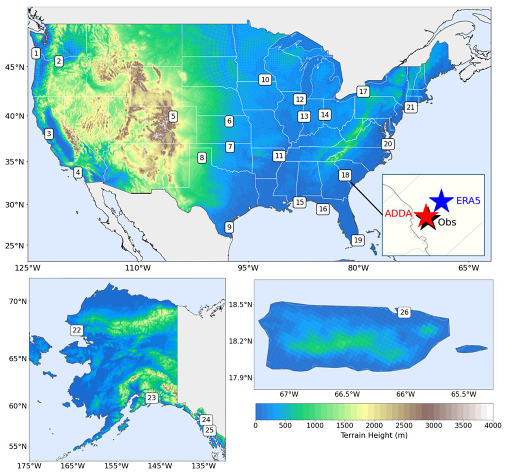
Figure 1 Locations of in situ observations sampled from meteorological towers across CONUS and Alaska, along with an ASOS location over Puerto Rico. The zoomed-in area, with stars representing each dataset, indicates the capability of ADDA v2's higher resolution to more closely match the exact location of the in situ data. The 2000+ sites over CONUS are not included here but can be seen in Fig. 6.

3.1.1 Probability density functions

PDFs effectively compare data distributions without considering the time dimension, aiming to visualize any biases between the model and observations. Across the 26 hub-height locations, ADDA v2's PDFs had a higher average OVL of 0.85 with the observational PDFs, while ERA5's PDFs had an average OVL of 0.78. Similarities between ADDA v2 and ERA5 distributions and observed wind speeds were spatially variable, with ADDA v2 performing better than ERA5 for 18 of the 26 sites considered. In particular, ADDA v2's higher resolution was able to capture the finer-scale wind speed patterns in mountainous regions, with OVLs significantly higher than ERA5's over the Cascades and the Rockies (Fig. 2c, d). ADDA v2 was able to modestly outperform ERA5 across the plain region. The average OVL for ADDA v2 across the nine locations was 0.86, while ERA5 saw an average OVL of 0.79. There were a couple of locations where both datasets struggled to capture the hub-height wind speed distribution. For example, both ADDA v2 and ERA5 demonstrated strong overestimations (Fig. 2j) for Spiderweb, South Carolina. As discussed in Sect. 3.3, ADDA v2's positive bias can be partly attributed to the land surface model (LSM) used for these simulations, as well as the positive bias inherited by ERA5. Both datasets also struggled with the hub-height wind speeds at Brookhaven, New York. However, the overestimations seen for this location by both datasets may be attributed to its unique geographic position; it is located on Long Island, New York, equidistant from Long Island Sound and the Atlantic Ocean, where land–sea interactions on either side may incite complexities in the local wind patterns. Across the four Alaskan locations, ADDA v2 saw an average OVL of 0.88 compared to ERA5's 0.70 (Fig. 2k). ERA5's coarser resolution can contribute to these errors, especially across Alaska, where complex topography incites stark spatial changes in wind patterns. For San Juan, Puerto Rico, ADDA v2 and ERA5 saw decent performance in capturing wind speed patterns, although both depicted modest overestimations (Fig. 2l).

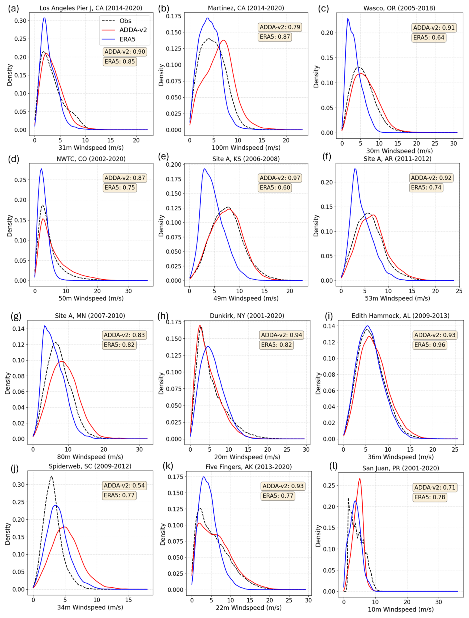
Figure 2 Probability density functions (PDFs) of wind speeds simulated by ADDA v2 and ERA5 alongside observations over Los Angeles Pier J, California (a); Martinez, California (b); Wasco, Oregon (c); NWTC, Colorado (d); Site A, Kansas (e); Site A, Arkansas (f); Site A, Minnesota (g); Dunkirk, New York (h); Edith Hammock, Alabama (i); Spiderweb, South Carolina (j); Five Fingers, Alaska; and (k) San Juan, Puerto Rico.

3.1.2 Mean bias

While PDFs provide a general view of a model's systematic bias, they do not evaluate the time dimension. Mean bias is therefore examined here to identify any systematic errors present within our models when considering the time dimension. Here, the entire overlapping time period between ADDA v2, ERA5, and the observations was taken. At each daily-averaged (Table 3), monthly-averaged, and seasonally averaged time step, the bias was taken between each dataset and observations. The interquartile range (IQR), minimums, and maximums of these bias values are then plotted in Fig. 3.

Table 3 Statistical metrics for each of the 26 hub-height observational locations.

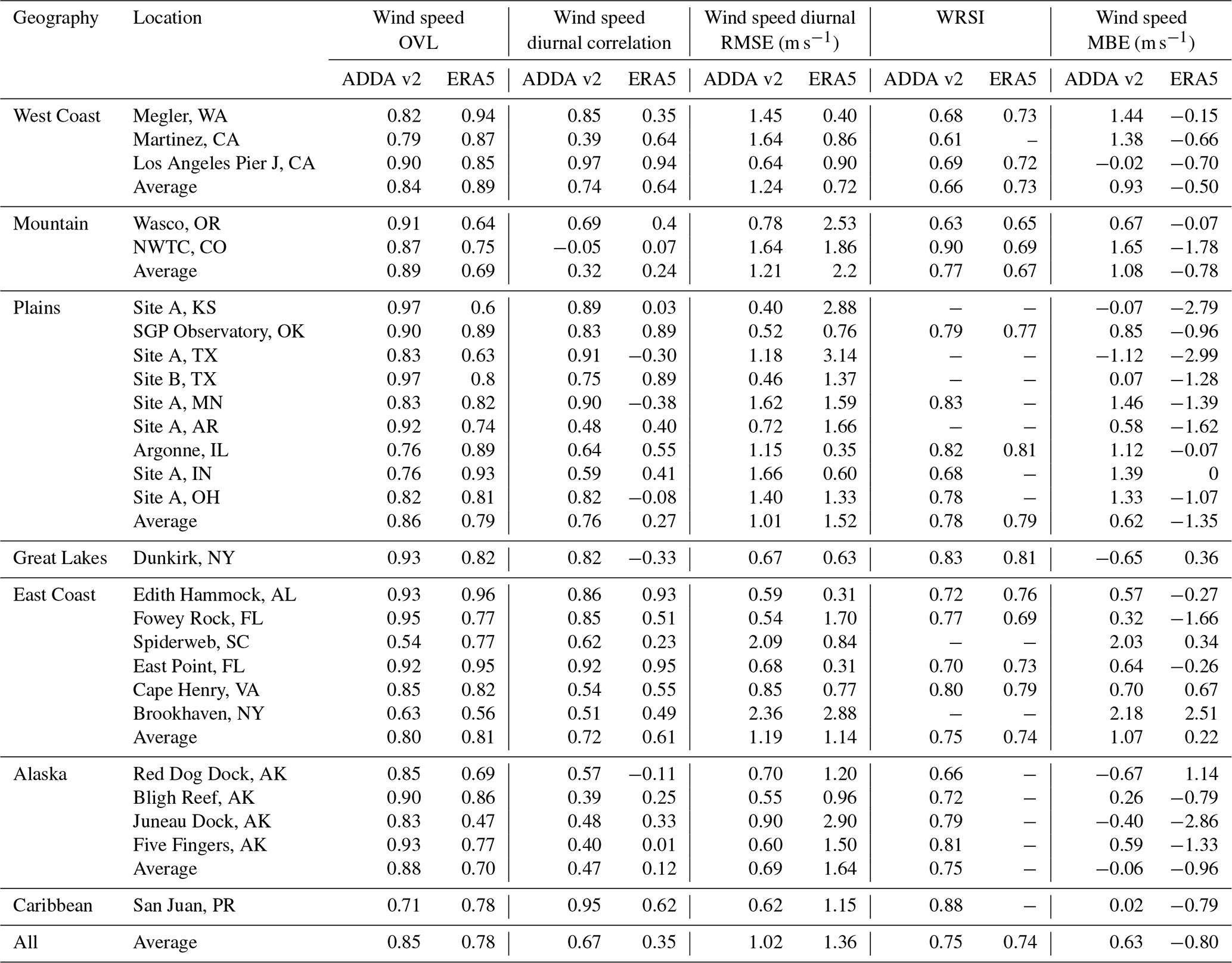
Figure 3 Distribution of mean biases computed between ADDA v2 (red) and observations and between ERA5 and observations (blue) during the overlapping time periods, plotted as box-and-whisker plots for Wasco, Oregon; Site A, Kansas; Fowey Rock, Florida; Five Fingers, Alaska; San Juan, Puerto Rico; and Los Angeles Pier J, California, at the daily (a), monthly (b), and seasonal (c) timescales.

Across most of the locations, ADDA v2's median biases are either centralized around 0 or slightly larger than 0, indicating that ADDA v2 performs reasonably well with slight overestimations. However, ERA5 demonstrated clear underestimations across the locations sampled. For example, for the mountainous location Wasco, Oregon, ERA5 saw a strong negative MBE (Fig. 3a). Similarly for the Great Plains location, Site A, Kansas, ERA5 saw an equally large negative MBE of −2.79 m s⁻¹. ADDA v2 had smaller MBEs for both locations at 0.67 and −0.07 m s⁻¹, respectively. The East Coast and Caribbean locations, Fowey Rock, FL, and San Juan, Puerto Rico, saw minimal MBEs of 0.32 and 0.02 m s⁻¹ for ADDA v2 and −1.66 and −0.79 m s⁻¹ for ERA5 (Fig. 3a). For Five Fingers, Alaska, MBE ranges were large for both ADDA v2 and ERA5 at the daily timescale. ADDA v2 outperformed ERA5 for this location, demonstrating a small positive bias compared to ERA5's modest underestimation. Lastly, both datasets had minimal MBEs for Los Angeles Pier J, California, with relatively small IQRs (Fig. 3a).

3.1.3 Diurnal cycles

While PDFs and mean biases are useful for understanding the overall distribution and temporal accuracy of model-simulated wind speeds, it is particularly crucial to understand how well the model captures diurnal variability in wind, especially when planning hybrid renewable energy assessments between wind and solar energies. Therefore, seasonally averaged wind speed diurnal cycles are considered in this analysis for each hub-height location to evaluate how well ADDA v2 captures intraday wind speed patterns. Specifically, an average was taken for each hour of the day (00:00, 01:00, 02:00 UTC, etc.) across each season. Wind speeds of 10 m were also included for some of these locations because they have more pronounced diurnal patterns. Pearson's r and RMSE values are used to validate the seasonally averaged model diurnal cycles.

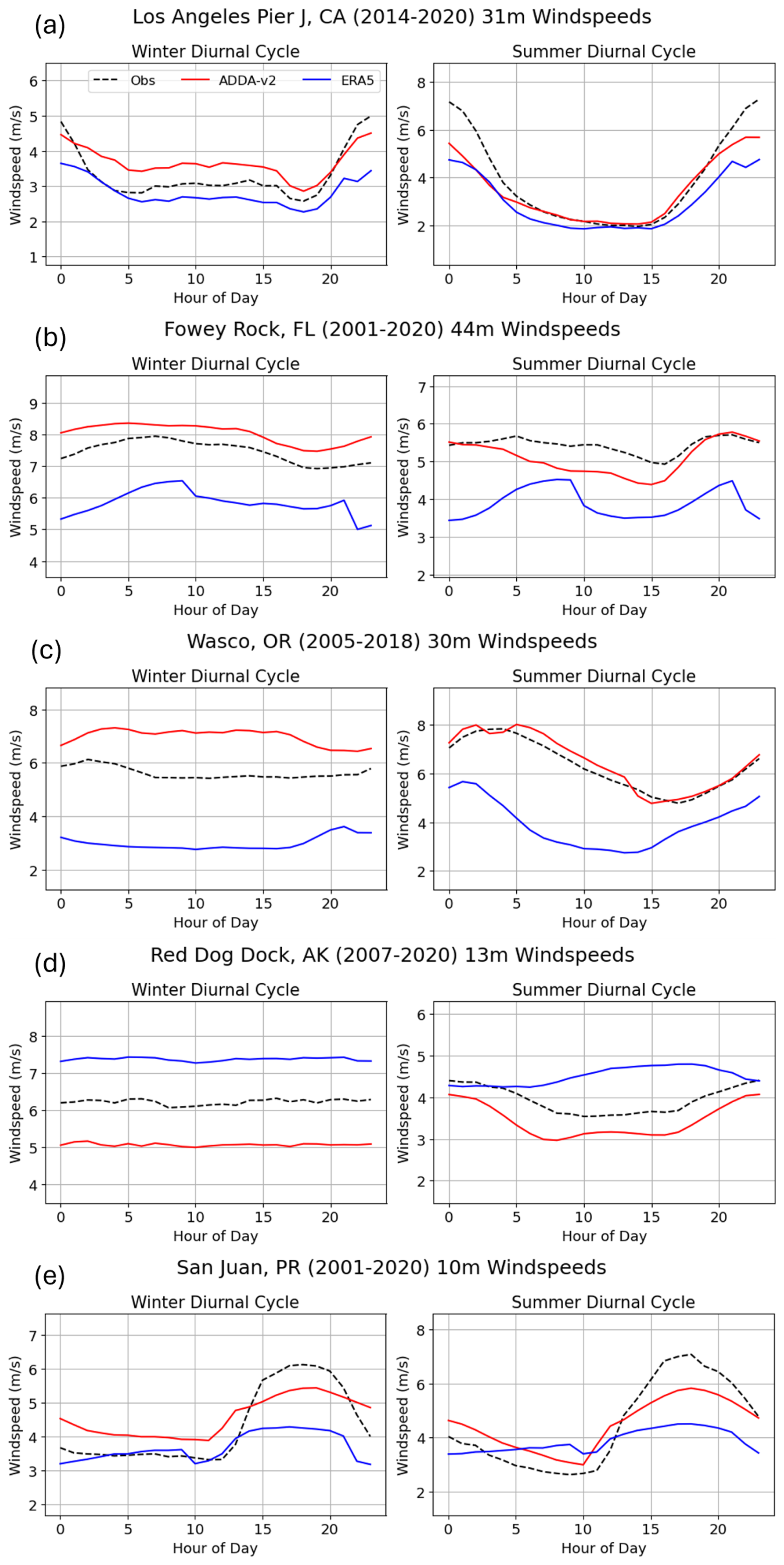
Figure 4 Seasonally averaged diurnal wind speeds (summer, winter) for Los Angeles Pier J, California (a); Fowey Rock, Florida (b); Wasco, Oregon (c); Red Dog Dock, Alaska (d); and San Juan, Puerto Rico (e).

Across all locations (Fig. 1), ADDA v2's diurnal wind speed patterns had an average Pearson's r of 0.67 with observations, while ERA5's average was considerably lower, at approximately r = 0.35. Similarly, ADDA v2 had a lower average RMSE of 1.02 m s⁻¹ compared to the 1.36 m s⁻¹ RMSE of ERA5. Both datasets saw improved performance when there was a strong diurnal signature in wind speed magnitudes, as summarized in Table 3. This was especially the case for southern locations, especially with coastal geographies, where the greater surface heating at lower latitudes modulates diurnal wind speed patterns more significantly (Elliott et al., 2004). For East Coast locations like East Point, Florida; Fowey Rock, Florida; and Edith Hammock, Alabama, Pearson's r values were at or above 0.85 for ADDA v2. ERA5 Pearson's r values were also high overall, but the dataset struggled with Fowey Rock in particular (Fig. 4b). Overall, ADDA v2 performed better for the wind speed diurnal pattern for the West Coast region (Fig. 4a), with an average Pearson's r of 0.74 compared to ERA5's 0.64. However, ADDA v2 did tend to overestimate wind speeds for Martinez, California, and Wasco, Oregon, leading to higher RMSE values compared to ERA5. For regions with flat terrain, ADDA v2 performed much better than ERA5. Correlation coefficients for plain-like geographies, on average, were r = 0.76 for ADDA v2 and r = 0.27 for ERA5. For mountainous regions, both ADDA v2 and ERA5 struggled significantly to capture diurnal wind speed patterns (Fig. 4c), with an average Pearson's r of 0.32 and 0.24, respectively. The high elevations of these locations have more complex responses to diurnal changes in solar heating and thus do not have very clear wind speed patterns throughout the day, especially during the winter (Fig. 4c). Across the four Alaskan locations, both datasets struggled to capture the diurnal pattern, with an average Pearson's r of 0.46 for ADDA v2 and 0.12 for ERA5. Lastly, for San Juan, Puerto Rico, both datasets were able to capture the dramatic diurnal wind speed pattern observed (Fig. 4e). However, ADDA v2 was much more precise, accurately simulating intraday wind speed minimums and maximums.

3.1.4 Wind roses

The previous sections focus on assessing model performance for wind speeds, but it is also important to assess model performance for wind direction to indicate whether the model can capture the synoptic-scale phenomena that drive these seasonal changes in wind direction. Wind direction is also important for understanding the wake effect in a large wind farm. This section employs wind roses to visualize seasonal wind direction distributions for each hub-height location between the model and observations.

Across the 19 locations that had wind direction data available, both ADDA v2 and ERA5 were able to capture the climatological synoptic mechanisms driving seasonal changes in wind directions reasonably well, with WRSIs at 0.75 and 0.74, respectively. No single geographic region within ADDA v2 significantly outperformed another, as summarized in Table 3.

However, ADDA v2 outperformed ERA5 for the mountainous location NWTC, Colorado, with WRSIs of 0.90 and 0.69, respectively. Here, ADDA v2 was able to accurately capture the predominantly western winds in the fall, winter, and spring, generated by mid-latitude cyclones and the more mesoscale chinook winds that occur on the leeward sides of mountain ranges (Lackmann, 2011; Markowski and Richardson, 2010). Diurnal patterns of wind direction were also evaluated (Fig. S1 in the Supplement). While both ADDA v2 and ERA5 captured the intraday wind direction patterns at the locations examined, ADDA v2 was able to simulate the wind direction shift in the afternoon during the summer more accurately, when wind direction has more abrupt changes due to diurnal heating and cooling, compared to ERA5.

Figure 5 Seasonally averaged wind speed and wind direction distributions for Los Angeles Pier J, California (a); Dunkirk, New York (b); Argonne, Illinois (c); and Cape Henry, Virginia (d). Values on each concentric circle (e.g., 4, 8, 12, 16) within the wind rose are used to measure the normalized frequency of each wind direction wedge. Wind rose wedge positions indicate the direction from which the wind is blowing.

Across the Alaskan locations, ADDA v2 performed moderately well, with wind direction WRSIs at Bligh Reef, Five Fingers, Juneau Dock, and Red Dog Dock (Fig. 5d) at 0.72, 0.81, 0.79, and 0.66. For coastal locations, like Red Dock, Alaska, summer wind directions can be influenced by sea breezes, indicated by the high frequency of southerly flow during the summer (Fig. 5d).

3.1.5 Model performance across various timescales

The model setup for ADDA v2 is designed to capture climatological statistics rather than to predict day-to-day weather (Appendix A in Wang and Kotamarthi, 2014). However, it can still be used to understand average intraday wind speed patterns for different regions. This section tests ADDA v2's capacity to represent wind speeds at different timescales using RMSEs and correlations, aiming to demonstrate the timescale at which the model can be useful for wind energy resource assessments.

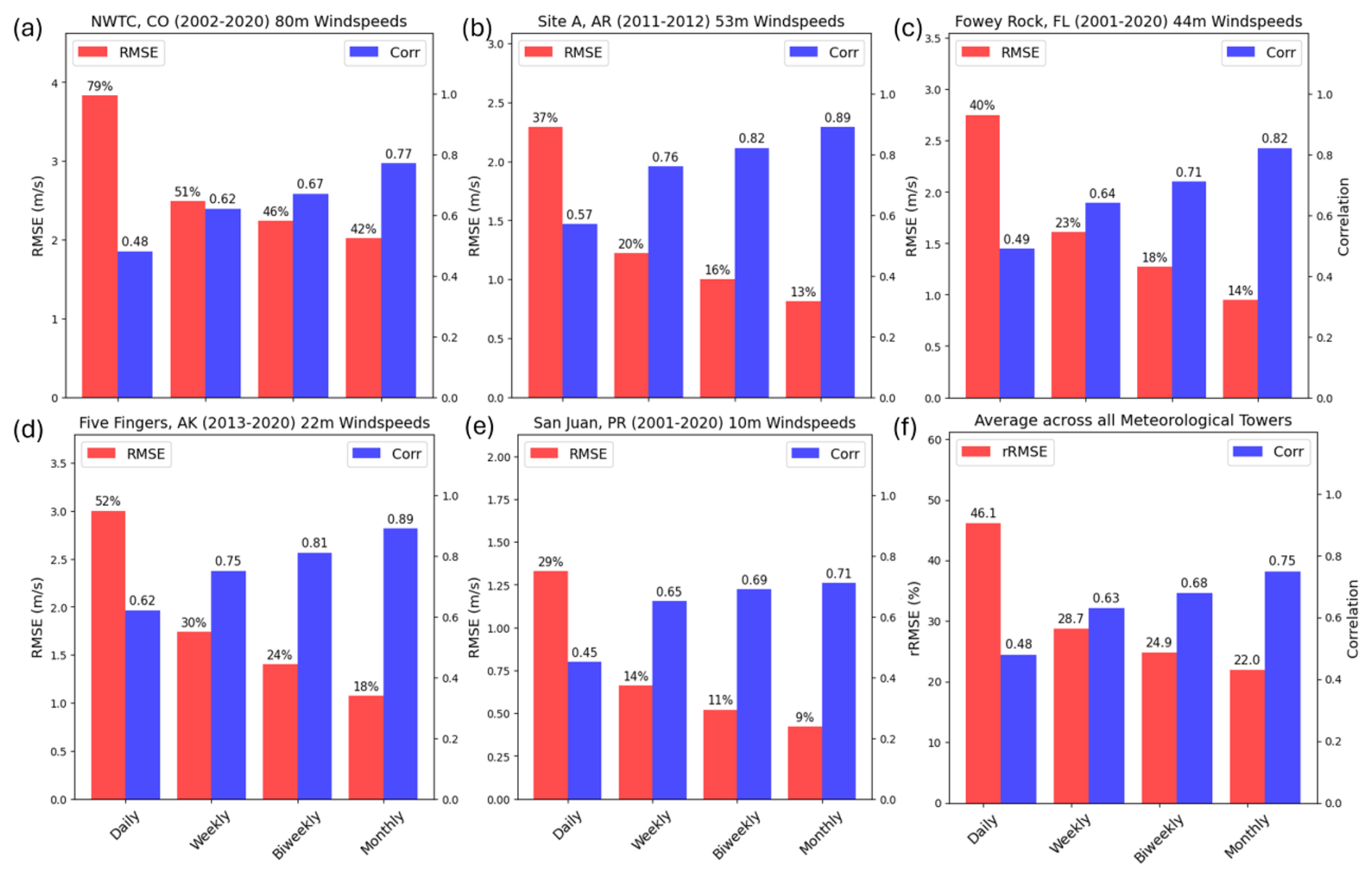
Figure 6 ADDA v2 RMSEs, rRMSEs, and Pearson correlation coefficients at different timescale averages for Site A, Arkansas (b); Fowey Rock, Florida (c); Five Fingers, Alaska (d); and San Juan, Puerto Rico (e), along with average metrics across all 26 meteorological towers (f). The number on each bar represents the value for each respective statistic, with timescales becoming coarser from left to right.

For almost all hub-height locations analyzed, RMSEs decreased and correlations increased as the timescale averages became coarser. On average across the 26 locations considered, rRMSEs at the daily, weekly, biweekly, and monthly scales were 46 %, 29 %, 25 %, and 22 %, respectively, indicating improvement at each transition to a coarser timescale (Fig. 6f). Pearson's r showed a similar trend, at r = 0.48, r = 0.63, r = 0.68, and r = 0.75 (Fig. 6f), consistently growing when calculated at increasingly coarse timescales. Moreover, the largest error improvement occurred when going from daily averages to weekly averages. For example, this can be seen for the 60 m wind speeds at Site A, Arkansas (Fig. 6b), where rRMSEs were at 37 % at the daily timescale, before dropping to 20 %, 16 %, and 13 % at the weekly, biweekly, and monthly timescales. Pearson's r also improved from 0.57 at the daily timescale to 0.89 at the monthly timescale. Similarly, Fowey Rock, FL (Fig. 6b), saw a drastic improvement from daily- to weekly-averaged wind speeds, with rRMSEs dropping from 40 % to 23 %, and Pearson's r steadily climbing between timescale averages. This trend is seen for the Alaskan and Puerto Rican locations as well, with ADDA v2 struggling to capture specific-day wind speeds but performing well at coarser, more climatological timescales (Fig. 6c, d).

3.2 Near-surface wind speed evaluation

ADDA v2 near-surface validations were initially performed using wind speed observations taken from 2000+ ASOS stations across CONUS, Alaska, and Puerto Rico. While the full temporal domain (2001–2020) of ADDA v2 was used in this analysis, statistics for each ASOS station were dependent on the maximum overlap in data availability between ADDA v2 and observations. Seasonal means were taken across the available temporal period before calculating the relative mean bias error (rMBE) and RMSE values for each ASOS station.

ADDA v2 performs well for the majority of ASOS stations evaluated, with rMBE values falling between −10 % and 10 % across much of the western and central portions of the model domain. However, ERA5 struggles significantly in these same regions, especially in the spring and summer (rMBEs upwards of −60 %). This has been documented in past studies (Chen et al., 2024; Wilczak et al., 2024), which highlight ERA5's tendency to underestimate wind speeds in areas of complex terrain (i.e., the Rockies).

For the eastern half of CONUS, both ADDA v2 and ERA5 show similar spatiotemporal patterns for error magnitudes. Specifically, both datasets demonstrate notable rMBE values across the southeast (60 %–80 %), most notably during the fall and winter. This systematic error is predominantly attributed to model overestimation during nighttime hours (00:00–12:00 UTC), when observational wind speeds are very low (0–1 m s⁻¹), which is at a scale typical of model uncertainty. Thus, when the model simulates wind speeds of about 1.5–2 m s⁻¹, the relative error appears significant. Interestingly, ADDA v2 also shows higher rMBE values for the upper Midwest during the fall and winter, when wind speeds are seasonally stronger; this bias is analyzed more in depth in Sect. 3.3. For most other regions, namely the central/lower Midwest, Texas, and the northeast, ADDA v2 and ERA5 accurately capture seasonal wind speeds, indicated by lower rMBE values.

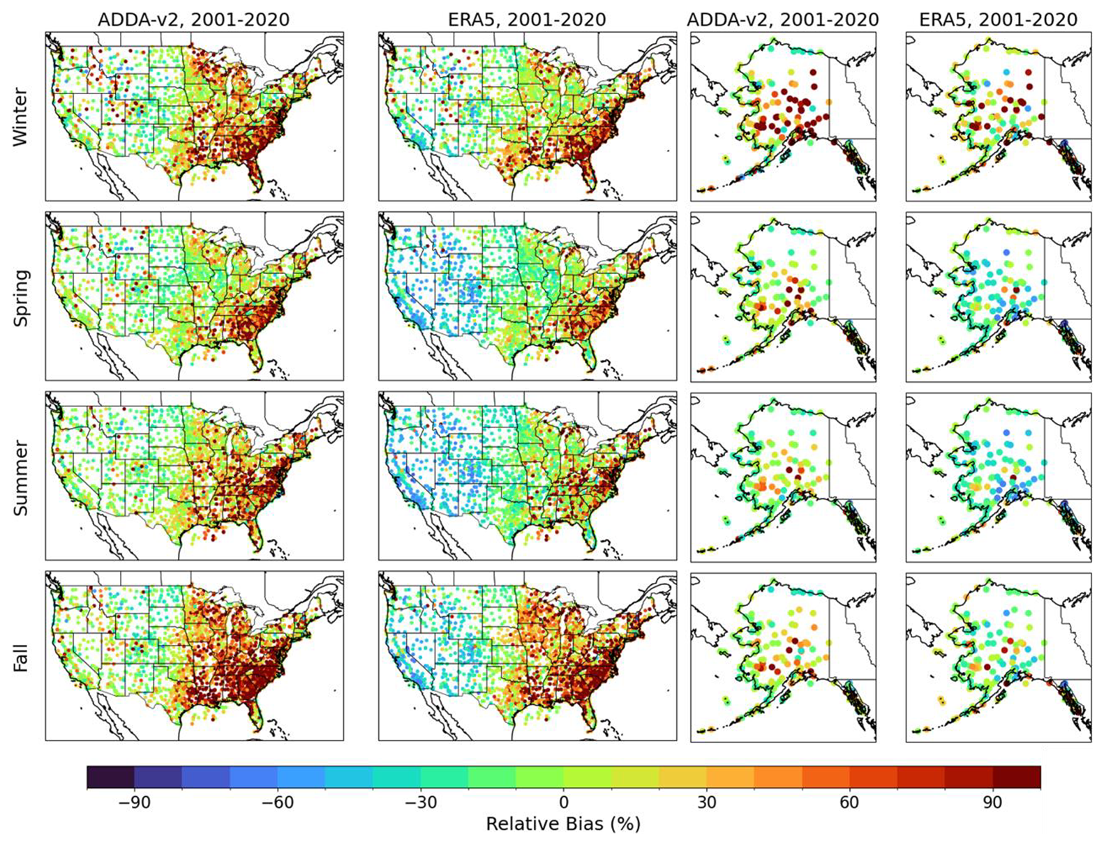
Figure 7 ADDA v2 and ERA5 seasonal rMBEs calculated against 2000+ ASOS locations across CONUS and Alaska.

When specifically looking at the ASOS stations over Alaska (Fig. 7), ADDA v2 and ERA5 generally capture coastal wind speeds well, with rMBEs of around −15 %–15 %, but struggle more in areas with complex topography. For some locations of Alaska's mountainous interior, rMBE values are much higher than those of surrounding locations (rMBEs around 60 %, especially during the winter). Overall, average RMSEs across Alaska for each season were 1.65, 1.08, 0.9, and 0.95 m s⁻¹ for ADDA v2 and 1.14, 1.23, 1.17, and 0.96 m s⁻¹ for ERA5. Similarly to CONUS, ADDA v2 was able to more accurately capture Alaska's wind speeds during the summer and fall but had a notable spike in RMSE magnitudes during the winter, especially for inland locations.

3.3 Sensitivity of wind speed biases to physics parameterizations

Given all the evaluations in previous sections, this section investigates some potential drivers of model bias over various regions, which can be used to implement solutions. Most notably, ADDA v2 sees positive wind speed biases across the southeast United States, as well as for some parts of the upper Midwest. This bias is seen for both the near-surface winds and the hub-height winds (Figs. 7, 2e). Part of these overestimations can be attributed to the biases within the forcing data of ERA5. Depicted in Fig. 7, ERA5 primarily overestimates wind speeds for southeast CONUS, especially during nighttime hours. Another potential reason for the overestimated wind speeds during nighttime could be attributed to the model's capacity to respond to atmospheric stability. It has been documented that Noah-YSU (the PBL and LSM schemes used to run ADDA v2 simulations) has enhanced performance for wind speeds in unstable conditions but struggles in a very stable atmosphere (Hong et al., 2006; Draxl et al., 2014; Wang and Jin, 2014). Thus, the very low wind speeds present during stable conditions may not be accurately captured by models employing these schemes.

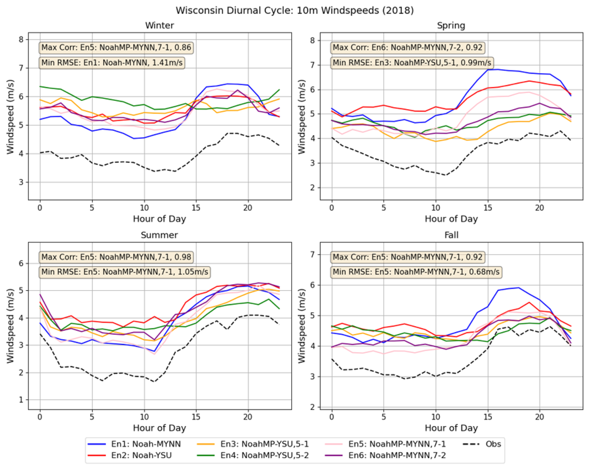
Figure 8 Seasonally averaged diurnal cycles for each of the structural uncertainty ensemble members (Sect. 2.4) against observed wind speeds in regions where ADDA v2 demonstrated a positive bias. Each ensemble label is denoted by its LSM or PBL scheme and the options for the dynamic vegetation and surface layer drag coefficient calculation (e.g., 5-1 means dveg = 5 and opt_sfc = 1 in namelist.input if NoahMP was used).

The overestimation of wind speeds over the upper Midwest, however, does not seem to be inherited from ERA5. Instead, it is likely due to the model's physics parameterization. Various ASOS locations were chosen in the Midwest, where ADDA v2 showed high error magnitudes, to examine whether different physics parameterizations minimized these errors. Seasonally averaged diurnal cycles were studied for these locations using the six structural uncertainty ensemble members (Sect. 2.2) with varying PBL and LSM schemes against observations. Error metrics were calculated, and the most accurate ensemble, indicated by the highest correlation coefficient or the lowest RMSE, was noted (Fig. 8).

For each location that demonstrated a positive near-surface wind speed bias, the NoahMP land surface model outperformed the Noah land surface model, as seen in the diurnal cycles plotted for a Wisconsin ASOS station (Fig. 8). It is also apparent that the greatest error occurs during overnight hours (00:00–12:00 UTC), in which none of the six ensemble members come close to representing the observed wind speeds. Contrarily, during daytime hours (12:00–00:00 UTC), all ensemble members more accurately capture wind speed magnitudes, although they still demonstrate some degree of overestimation. Furthermore, in all but one metric, the MYNN PBL scheme outperformed the YSU PBL scheme. Of the statistical metrics considered for each season, the MYNN PBL scheme almost always showed the lowest RMSE value and the highest correlation coefficient. However, it is important to acknowledge that no individual model configuration was able to solve the positive bias seen for these locations.

Considering the effects that different LSM schemes have on simulated wind speeds, we further analyzed how specific LSM parameterizations drive differences in near-surface winds. One of the most important considerations is friction velocity, typically denoted by u_∗. Friction velocity quantifies the turbulent momentum flux at the surface. Therefore, higher u_∗ values correspond to more of the momentum being lost to the surface, leading to weaker wind speeds closer to the ground.

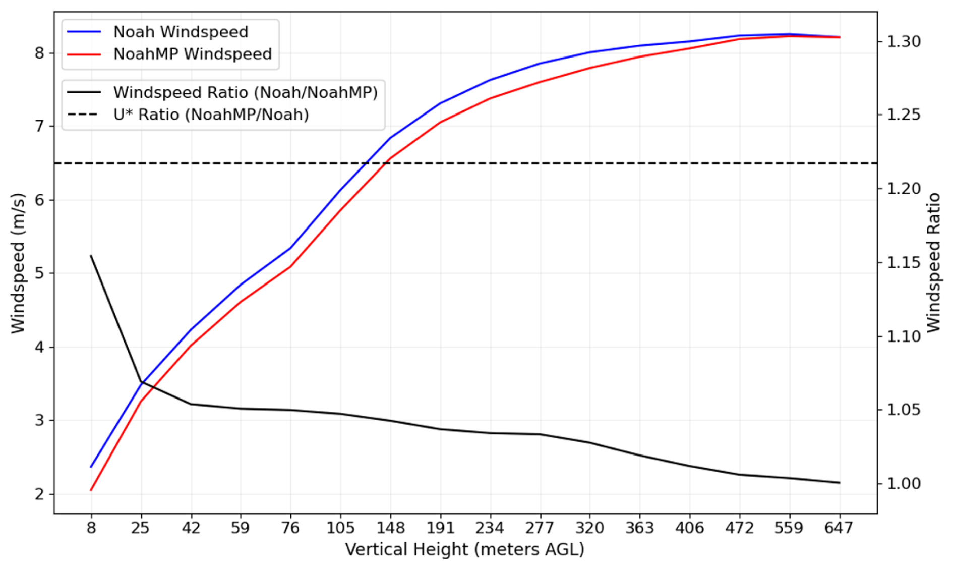
Figure 9 Vertical profile of wind for a location in which ADDA v2 overestimated wind speeds, comparing averaged winds between the 2018 simulations using the NoahMP and Noah LSMs. Wind speed profiles correspond to the leftmost y axis, while the ratios of both wind speed and friction velocity use the rightmost y axis.

We analyzed u_∗ between the NoahMP and Noah LSM schemes and found that friction velocity generally tends to be larger in model simulations that employ NoahMP (Fig. 9), especially at the locations that saw positive near-surface wind speed biases. In some cases, the friction velocity was as much as 20 %–25 % larger in NoahMP than in Noah. As a result, as shown in Fig. 9, wind speed ratios between NoahMP and Noah, specifically within the first ∼ 10 m a.g.l., were as high as 1.15 (Fig. 9). At greater heights (e.g., 25 m and above), this ratio decreases as friction has a diminishing influence on momentum fluxes with increasing height as wind speeds get stronger overall. Therefore, while the NoahMP LSM saw improved performance in simulating near-surface winds, it still did not fully resolve the positive bias observed.

3.4 Interannual variability and model uncertainty

Interannual variability across ADDA v2's 20-year temporal period was calculated across the entire spatial domain. Additionally, model uncertainty was quantified by investigating the spread across 500 augmented ensembles, varying in their physics parameterizations (structural uncertainty) and initial conditions (internal variability). While the model uncertainty brought about by structural uncertainty was larger than that generated by the internal variability (Fig. S2), both were considered here to provide a comprehensive view of all model uncertainty. The magnitudes and spatiotemporal patterns of each of these variabilities are then investigated here. Intuitively, the degree of model uncertainty is significantly influenced by the timescale being analyzed. This can be seen in Fig. 10, in which the magnitude of uncertainty scales inversely with the length of the timescale. The biweekly, weekly, and daily timescales see overall uncertainty values of approximately 0.4–0.7, 0.7–1.1, and greater than 2.5 m s⁻¹, respectively, across much of North America (Figs. 10, 11). This concept is similar to the improved performance of ADDA v2 at coarser-resolution timescales (Sect. 3.1.4). We also found that nighttime uncertainties were slightly higher than daytime uncertainties in regions of complex topography, especially over the Rocky Mountains.

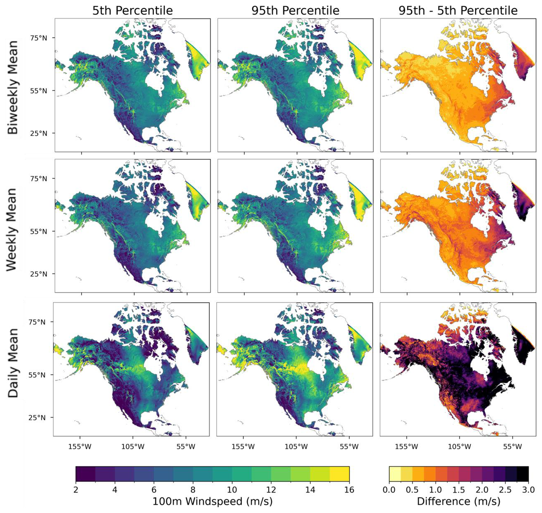
Figure 10 Model uncertainty at different timescale averages (daily, weekly, and biweekly). For a detailed description of the methodology for uncertainty quantification, see Sect. 2.5.

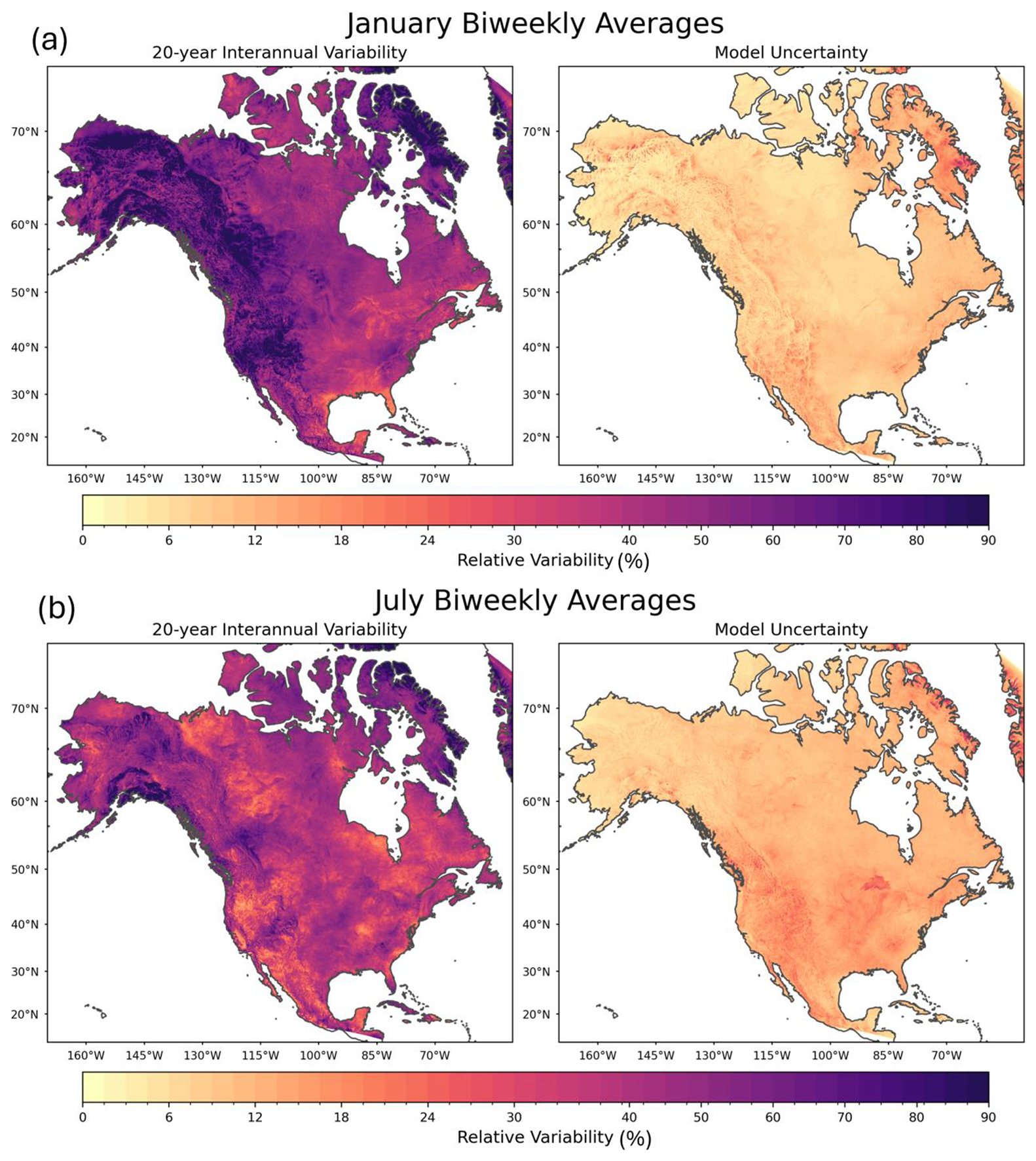
Figure 11 Relative interannual variability and relative model uncertainty for one biweekly-averaged period for a winter month (January) and a summer month (July) for 100 m wind speeds. For a detailed description of the methodology for interannual variability quantification, see Sect. 2.5.

In terms of the spatial patterns of model uncertainty, the mountainous regions generally demonstrate higher uncertainty values, by about 0.5 m s⁻¹, when compared to adjacent regions with simpler topography (Figs. 10, 11a, b). This indicates that complex terrain introduces more unpredictable interactions between the physical mechanisms that drive near-surface and low-level winds (Wu et al., 2022a; Helbig et al., 2017). These interactions pose challenges for the model in producing reasonable solutions. Thus, small changes in model initial conditions or parameterizations can influence these mechanisms and cause significant variability within the simulated wind. It is also interesting to note that large lake features also observed high degrees of model uncertainty, specifically during the summer months, indicating the model's inadequacy in solving air–lake interactions and the need for a fully coupled lake–atmosphere model (Kayastha et al., 2023).

In the context of wind energy applications, model uncertainty is integral when mapping ideal locations for wind farm siting. However, it needs to be paired with spatiotemporal patterns of interannual variability to understand the full scope of wind resource reliability and potential risks associated with long-term power generation. Ideally, both model uncertainty and interannual variability need to be low for optimal and consistent power generation. As seen in Fig. 11a and b, the relative magnitude scale of interannual variability and model uncertainty is very different for all seasons. For example, the interannual variability of biweekly-averaged 100 m wind speeds can be as high as 70 %–80 % of the wind speeds themselves. This is observed especially during the winter months, when highly variable synoptic-scale features strongly influence wind patterns. Alternatively, model uncertainty exists at a smaller magnitude, typically in the range of about 10 %–20 % of the mean wind speed.

The interannual variability in summer is smaller, with typical magnitudes ranging from 30 %–40 % of the mean wind speed, likely attributable to the more consistent synoptic patterns present during summer. At coarser timescales (e.g., seasonal), both interannual variability and model uncertainty decrease considerably. Across much of North America, seasonal interannual variability is 15 %–25 % of the mean wind speed. But, consistent with any timescale, these values can be as high as 40 %–50 % in regions of complex topography (Fig. S3).

The short-term ensemble simulations can be leveraged with the long-term simulations to identify key regions that have an optimal combination of moderately strong wind speeds and relatively low model uncertainty and interannual variability. Ultimately, this will maximize energy output potential for optimally sited wind farms.

4 Discussion and concluding remarks

The validation of the Argonne Downscaled Data Archive version 2 (ADDA v2) dataset presented in this study underscores its utility in wind resource assessments and climatological applications. This section synthesizes the key findings and compares the performance of ADDA v2 with ERA5, highlighting ADDA v2's added value to its coarser-resolution forcing data.

ADDA v2 demonstrated significant advantages over ERA5 in capturing fine-scale wind variability across diverse geographies. The dataset performed particularly well in regions with complex terrain, such as the Rocky Mountains and Alaska, where high-resolution modeling captured localized wind phenomena more effectively. This is especially critical when assessing the consistency in wind power generation throughout the day, with potential implications for hybrid-style energy generation. Additionally, ADDA v2's ability to reduce errors at coarser temporal scales (e.g., weekly and monthly averages) reinforces its applicability to long-term climatological studies and resource planning. However, challenges remain, particularly in regions where both ADDA v2 and ERA5 struggled, such as the southeast United States and areas characterized by stable atmospheric conditions. These limitations highlight the need for targeted improvements in existing and new parameterizations (e.g., PBL and LSM) to address specific biases. Additionally, while this validation focused more on inland regions, Sheridan et al. (2025) have evaluated ADDA v2's performance over coastal locations. Tobias-Tarsh et al. (2025) have evaluated ADDA v2's performance in wind-related extremes in the context of tropical cyclones over the North Atlantic Basin.

Other studies exist that introduce wind datasets and validate them against observations. For instance, Draxl et al. (2015b) documented a 7-year wind dataset with a grid spacing of 2 km, primarily focused on wind power evaluations over CONUS, and included a limited meteorological validation using six tall masts and three buoys. Rasmussen et al. (2023) performed validations on a 42-year-period, 4 km dataset of near-surface (10 m) wind speeds, with underestimation particularly over complex terrain. While these datasets provide their own unique utility, ADDA v2 offers a powerful combination of a reasonably long time period and a large spatial domain containing unique geographic regions. By comprehensively validating ADDA v2's wind speeds and directions using an extensive network of near-surface observations and a diverse set of hub-height observations, this evaluation can provide insight for both climatological studies and wind resource assessments. Yet, all these datasets can be used collectively, complementing one another with their unique characteristics and allowing for a more comprehensive view of model uncertainty and longer-term variability.

However, even with all these datasets developed thus far, it is challenging for high-resolution numerical simulations covering such large domains to capture all model uncertainty and variability. The experiments presented here aim to deliver a relatively robust sample of model uncertainty, but there are many other physics parameterizations that can generate different model solutions. Recent advances in machine learning (ML)-based surrogate models or hybrid models may provide a more comprehensive means of quantifying model uncertainty (Tunnell et al., 2023; Di Santo et al., 2025; Pringle et al., 2025) given that they can perform faster calculations.

While this evaluation demonstrates the capabilities of ADDA v2 in capturing climatological features using multiple metrics over various geospatial locations, some other features can be investigated in future work. One of them is the spatial and temporal variability captured by the model. As demonstrated by past studies (e.g., Müller et al., 2024; Skamarock, 2004; Larsén et al., 2012), atmospheric models with spatial resolution Δx can only capture the energy spectrum at wavelengths ∼ 4–6 Δx. Thus, at a 4 km model resolution, the inherent variability and turbulence of the atmosphere can only be simulated accurately at ∼ 20 km scales (Kolmogorov, 1941; Durran, 2010; Skamarock et al., 2008). Evaluation of such variability would require continuous gridded observational data, such as those from radar, lidar, or satellites (Müller et al., 2024). Another consideration for future work is to make the evaluations more robust by including multiple model grid cells surrounding each observation site, rather than using only the closest grid cell, as we did in this study. This would allow us to characterize a range of modeled winds around the observation sites and better represent model spatial variability. Lastly, while this study prioritizes climatology inland, future work is needed to analyze ADDA v2's capability of capturing extreme winds, which can provide insight into storm-related (e.g., derechos) risk assessments (Li et al., 2025).