Flow field analysis of a leading-edge inflatable kite rigid-scale model using stereoscopic particle image velocimetry

Leading-edge inflatable (LEI) kites exhibit pronounced anhedral and pressure-side recirculation associated with their double-curved geometry and tubular frame. This study reports wind tunnel stereoscopic particle image velocimetry (PIV) measurements around a rigid 1:6.5 scale model of the TU Delft V3 kite. Measurements are acquired in chordwise planes located between the mid-span and tip at two angles of attack and are compared against slices extracted from Reynolds-averaged Navier–Stokes (RANS) simulations at corresponding spanwise positions. Reflection-prone surface geometry required tailored masking and an additional out-of-plane velocity filter, leaving near-wall data in the pressure-side recirculation region unresolved. Sectional lift and drag were estimated using the Kutta–Joukowski relation, RANS surface pressure integration, and Noca's method. Within the Noca framework, reliable lift and physically consistent drag are obtained only from specific inviscid contributions, indicating that selective use of individual terms is more robust than applying the full formulation in the present configuration. Local discrepancies near strut junctions are consistent with three-dimensional (3D) strut-induced flow effects observed in computational fluid dynamics (CFDs), which are captured by surface pressure integration but not by contour-based planar methods. Comparison confirms agreement between PIV and CFD to within 5 % of the freestream velocity across the majority of the flow field, and circulation distributions obtained from contour integration show consistent spanwise trends between the vortex step method, RANS, and PIV, jointly supporting the use of the dataset as a valuable, albeit not definitive, validation resource for aerodynamic models of LEI kites.

1 Introduction

Leading-edge inflatable (LEI) kites are used for kite-surfing and novel renewable energy applications such as wind-assisted ship propulsion and airborne wind energy (AWE). This specific type of kite uses an inflated tubular frame to collect the aerodynamic load generated by a canopy and to transmit this via a system of bridle lines to one or more tethers. Their design as a single morphing aerodynamic control surface makes LEI kites highly manoeuvrable, which is a crucial requirement for the mentioned applications (Breukels, 2011). Pitch control is achieved by symmetric actuation of the bridle line system (Hummel et al., 2019) and directional control by asymmetric actuation (Elfert et al., 2024). The wings are generally downwardly curved to minimize the spanwise stresses in the bridled membrane structure. While the vertical wing area contributes to the favourable yaw authority, with the sweep of the wing extending the depower range of the kite. In addition to the actuation-induced morphing, the shape of the membrane wing is also subject to aero-structural coupling effects. The kite investigated in the present study is illustrated in Fig. 1 and described in more detail by Oehler and Schmehl (2019).

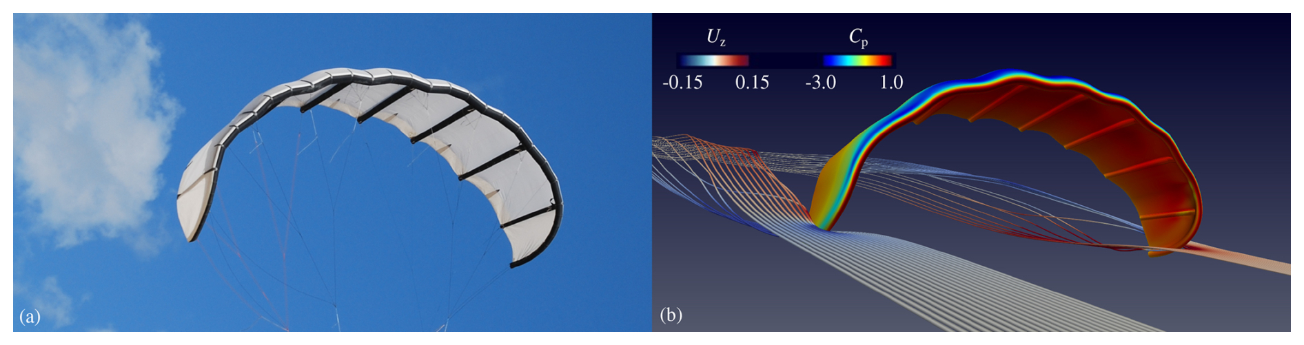
Figure 1 TU Delft V3 kite designed for AWE harvesting: (a) 2012 prototype with a flat wing surface area of 25 m² and (b) CFD visualization of the flow around the design geometry, depicting the non-dimensional surface pressure C_p on the wing and the flow velocity z-component U_z colouring streamlines along the flow around the wing tips (adapted from Viré et al., 2022).

Characterizing the aerodynamics of LEI kites using numerical prediction and experimental measurements poses challenges associated with structural flexibility, pronounced anhedral and sweep, and unconventional airfoil geometries. A representative example is the discontinuity at the junction between the inflated leading-edge tube and the attached single-skin canopy, which promotes pressure-side separation and recirculation even at low angles of attack. Consequently, fast potential flow solvers cannot be used to analyse the two-dimensional (2D) aerodynamics, as was demonstrated in our companion paper (Poland et al., 2026a). Instead, computational fluid dynamic (CFD) solvers based on Reynolds-averaged Navier–Stokes (RANS) equations have to be employed, substantially increasing the computational resource demands for early design iterations (Folkersma et al., 2019). To avoid this computational overhead, which can become excessive when the wing geometry changes continuously, Breukels (2011) derived polynomial approximations of the sectional aerodynamic coefficients C_l, C_d, and C_m from CFD simulations of a large variety of parameterized LEI airfoil shapes. In our companion paper (Poland et al., 2026a), we refined the airfoil parameterization and used machine learning to develop regression models with a wider parametric range. To expand the 2D aerodynamic properties to three-dimensional (3D) wings, lifting-line methods (Leloup et al., 2013) and vortex step methods (VSMs) (Damiani et al., 2019; Cayon et al., 2023) have been used successfully. In particular, the implementation of precomputed, shape-dependent airfoil aerodynamic coefficients in the VSM framework deliver high-quality results (Poland et al., 2026a). RANS simulations of complete LEI kites have also been conducted, with parametric sweeps in Reynolds number, angle of attack, and sideslip angle, indicating that the strut tubes exert a negligible influence on the integral aerodynamic properties (Viré et al., 2020, 2022).

Experimental analyses of kite aerodynamics are generally most reliable when conducted in a wind tunnel under controlled flow conditions (De Wachter, 2008; Desai et al., 2024). However, industrial-scale kites in the size range of 50 to 500 m² cannot be mounted at full scale in wind tunnel facilities. On the other hand, reverting to scale models requires preserving aeroelastic similarity, which is challenging for a bridled inflatable membrane structure. A practical option is to decrease the complexity of the fluid–structure interaction problem by investigating the aerodynamics of a rigid-scale model, such as that presented by Belloc (2015) for a reference paraglider wing. A similar approach was pursued in our companion paper (Poland et al., 2026b), where the aerodynamic loads on a rigid-scale model of the TU Delft V3 kite were measured for different angles of attack, sideslip angles, and Reynolds numbers. The measured forces and moments corroborate numerical predictions from CFD and VSM simulations within the nominal operating regime, encompassing angles of attack from 2 to 8° and sideslip angles of ±10°, as reported by Cayon et al. (2025).

Although numerical studies have significantly advanced the understanding of LEI airfoil aerodynamics and integral effects of airfoil loading, a detailed experimental analysis of the sectional flow around this class of wing has not been reported in the literature. Particle image velocimetry (PIV) offers a non-intrusive method to capture planar flow fields, with minimal influence from introduced tracer particles. Stereoscopic PIV, employing two cameras, mitigates potential errors caused by perspective distortions in velocity measurements (Prasad, 2000). The resulting flow fields enable evaluation of local pseudo-2D aerodynamic properties, including circulation, induction, inflow angles, forces, and aerodynamic coefficients (Fritz et al., 2024a). Circulation can be determined by defining a boundary curve and interpolating velocity components along it, and forces may subsequently be estimated on this boundary using Noca's method (Noca et al., 1999).

The present study addresses this gap by providing stereoscopic PIV measurements in chordwise planes along the span of a rigid TU Delft V3 scale model at two angles of attack, forming the first geometry-consistent, spatially resolved flow field dataset for a representative LEI kite configuration. The resulting measurements enable qualitative and quantitative comparison with RANS CFD and VSM predictions, supporting their use in sectional and spanwise load modelling. Although stereoscopic PIV is well established, its application to the strongly anhedral LEI geometry, characterized by extensive pressure-side recirculation, has not been previously documented.

The remainder of the paper is organized as follows. Section 2 describes the experimental methodology, including the wind tunnel, rigid-scale model, experimental setup, stereoscopic PIV technique, test cases, data processing, and methods for deriving aerodynamic quantities. Section 3 presents the results, including uncertainty analysis, qualitative comparisons between CFD and PIV, and quantitative comparisons. A discussion of the results follows in Sect. 4, addressing PIV measurement limitations, an analysis of quantitative discrepancies, and local strut effects. Conclusions and recommendations for future research are presented in Sect. 5.

2 Method

This section outlines the specifications of the wind tunnel, the scale model, the experimental setup, and the PIV technique. The arrangement of the measurement planes is discussed next, followed by the data-processing steps and a description of how integral aerodynamic quantities are derived from planar flow field data.

2.1 Wind tunnel

The wind tunnel experiments were conducted in the closed-loop Open Jet Facility (OJF) of the TU Delft from 8 to 12 April 2024. The tunnel has an octagonal exhaust nozzle measuring 2.85 m × 2.85 m and is equipped with a 500 kW electric motor and a large fan generating a flow speed of up to 35 m s⁻¹. To ensure uniform flow conditions in the test section, the tunnel uses corner guide vanes and wire meshes. The maximum reported turbulence intensity in the test section is 0.5 % (Lignarolo et al., 2014). The PIV measurements used a wind speed of U_∞ = 15 m s⁻¹, with variations from the set point up to 0.2 %. The inflow and atmospheric conditions for each measurement were logged to enable correct non-dimensionalisation of the data. This was particularly important in this campaign as the temperature ranged from 22 to 32 °C due to a malfunctioning cooling system.

The projected frontal blockage ratio is approximately 3 %, for which blockage-induced acceleration and the associated correction to the effective angle of attack are expected to be small (Poland et al., 2026b). This assessment is consistent with common wind tunnel guidance recommending blockage ratios below 7.5 % (Barlow et al., 1999). In the OJF, the jet is bounded by turbulent shear layers that originate at the nozzle edges and contract the jet core with a reported semi-angle of 4.75° near the nozzle exit (Lignarolo et al., 2014). With the model centred in the 2.85 m nozzle and a model width of 1.28 m, the wing tips remained approximately 0.8 m from the nozzle edge.

Table 1 Corrections for angle and drag coefficients (Poland et al., 2026b).

On this basis, open-jet shear layer effects and blockage corrections are considered to be negligible for the present dataset. By contrast, streamline curvature effects measurably modify the effective angle of attack; the corresponding correction values are reported in Table 1, with the underlying analysis documented in the companion paper (Poland et al., 2026b). These corrections are applied to all reported α values.

2.2 Rigid-scale kite model

A rigid wing was used to decouple aerodynamics from aeroelasticity, enabling geometry-consistent, well-controlled measurements that provide unambiguous validation data for numerical models. Such a one-to-one comparison is not feasible for a scaled, flexible AWE-sized kite wing because aeroelastic similarity cannot be preserved: simultaneous matching of Reynolds number, mass distribution, structural stiffness, membrane pretension, and damping is not achievable in a practical wind tunnel setup. The rigid configuration isolates the aerodynamic response of a well-defined reference geometry so that discrepancies between measurements and simulations can be attributed primarily to aerodynamic modelling assumptions rather than to uncertain, unmeasured deformation states.

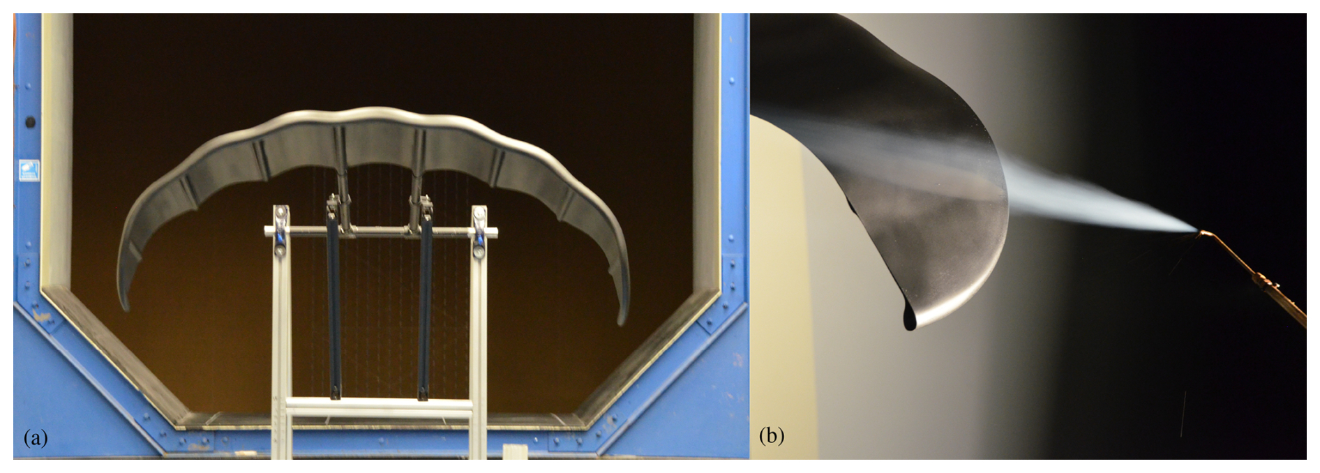
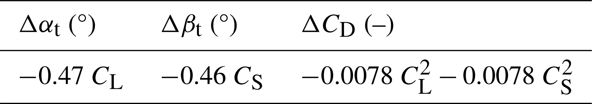
Figure 2 Wind tunnel setup: (a) rigid-scale model in the wind tunnel, swivelled by 180° with its back facing the octagonal OJF exhaust nozzle. (b) Rear view showing a smoke trail visualization of the flow over a wing tip and indicating the fillet between the circular leading edge and the canopy.

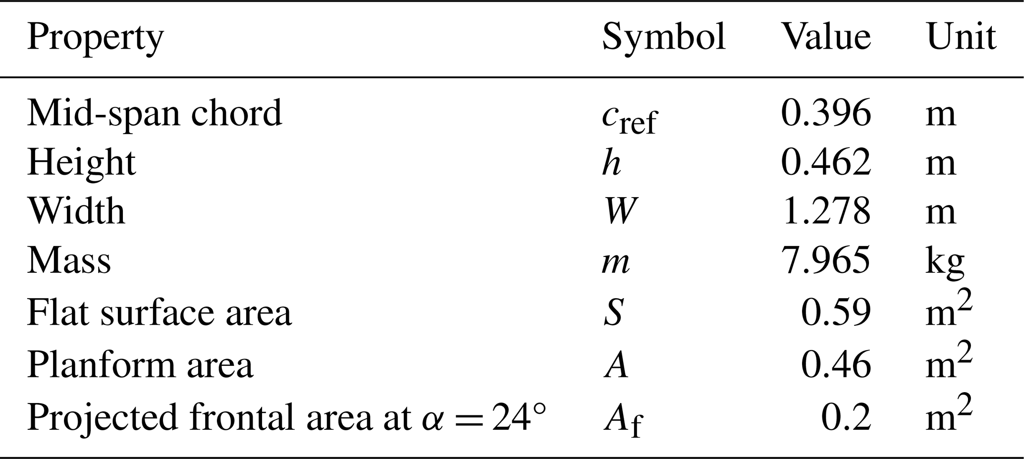
To manufacture a rigid-scale model of the V3 kite, the wing geometry adapted for the CFD simulations by Viré et al. (2022) was used, as detailed in the companion paper (Poland et al., 2026b). This CFD geometry differed slightly from the original design: the bridle line system was omitted, the trailing edge connecting the upper and lower wing surfaces was rounded, and edge fillets were applied to all tubular frame-to-canopy connections. Using the CFD geometry was motivated by the intended purpose of the measurement data: validating computational studies. The wing was scaled down by a factor of 1:6.5, resulting in the dimensions outlined in Table 2, and the Reynolds number

$$\begin{array}{}\text{(1)}& \mathit{Re}={\displaystyle \frac{\mathit{\rho }{U}_{\mathrm{\infty }}{c}_{\text{ref}}}{\mathit{\mu }}}=\mathrm{3.8}\times {\mathrm{10}}^{\mathrm{5}},\end{array}$$

where ρ = 1.2 kg m⁻³ denotes the density, U_∞ = 15 m s⁻¹ denotes the inflow speed, c_ref = 0.396 m denotes the reference chord, and μ = 1.89 × 10⁻⁵ denotes the dynamic viscosity. The scale model mounted in the test section is shown in Fig. 2a, with a rear view of the wing tip in Fig. 2b. The image highlights the smooth transition between the circular leading-edge tube and the membrane surface. Although the idealized CFD geometry also incorporates fillets in this region, the manufactured scale model exhibits slightly larger radii due to manufacturing constraints.

Table 2 Dimensions of the 1:6.5 scale model. Chord length, height, and width of the manufactured model deviate by no more than 1 mm from the scaled geometry, as verified using a laser tracker (Poland et al., 2026b).

2.3 Experimental setup

The scale model is positioned in the centre of the octagonal jet exhaust using a support structure of aluminium beams. Two steel rods extend from the wing's centre struts and connect the scale model to the support frame, as shown in Fig. 2a and detailed in the companion paper (Poland et al., 2026b). The images in Fig. 3 depict the normal and upside-down configurations, respectively, for analysing the flow field on both sides of the wing with the cameras positioned on the ground. The highlighted horizontal bar was used to adjust the angle of attack α of the wing, achieving an accuracy of 0.1° as measured by digital inclinometers. Both the cameras and the laser were mounted on a motorized traverse system with a step size of 0.01 mm in the x and y directions. This configuration permitted measurements at multiple chordwise (x) and transverse (y) locations without the need to refocus the cameras or recalibrate the software. Due to the wing's downward curvature, the distance between the PIV system and the measurement plane varied. To ensure that the wing remained within the camera field of view, its vertical position was adjusted for certain measurements by raising the blue table supporting the structure, as shown in Fig. 3.

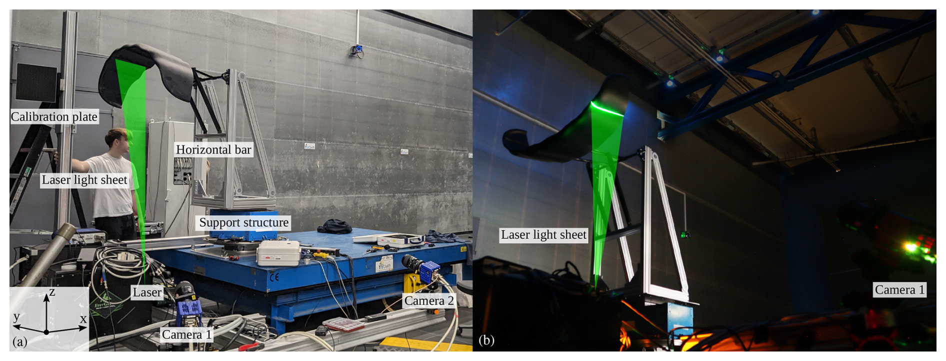
Figure 3 Experimental setup: (a) photograph showing the labelled components of the setup and the axis orientations. (b) Long-exposure photo of the laser light sheet projected onto the model. In this instance, the laser light sheet spans the entire chord, a coverage not typical during standard measurements, achieved here by operating the system in laser alignment mode. In both photos, the laser light sheet was graphically enhanced.

2.4 Stereoscopic particle image velocimetry

The flow field around the wing was measured non-intrusively with stereoscopic PIV. The flow, seeded with tracer particles, was captured by two synchronized cameras, each recording pairs of images with a time delay of 100 µs. The flow field was determined by comparing these sets and tracking the displacement of particle groups. Laser control, camera synchronization, and image acquisition were all triggered by a single pulse signal from an opto-coupler (TCST 2103), controlled via LaVision's DaVis 8 software. For each plane, each camera recorded a total of 250 image sets at 15 Hz, which, as demonstrated in Fig. A1 in Appendix A, was sufficient to ensure statistical convergence for time-averaged results.

A Quantel Evergreen double-pulsed neodymium-doped yttrium aluminium garnet laser was used as the light source, with a wavelength λ_L of 532 nm, shaped into an approximately 3 mm thick laser light sheet. As illustrated in Fig. 3, the generated vertical light sheet illuminates a flow-aligned cross-section of the floor-facing side of the wing. To reduce light reflections, both the wing and relevant parts of the support structure were spray-painted matte black. A Safex smoke generator produced tracer particles with a median diameter of 1 µm. The generator was positioned downstream of the tunnel test section to ensure a homogeneous mixing of the particles with the flow before re-entering the test section.

The two LaVision Imager sCMOS cameras, with an f number f_#=8, defined as the ratio between focal length and aperture diameter (Raffel et al., 2018), were placed at radial distances of 1.70 and 1.95 m from the laser light sheet. This configuration resulted in a field of view (FOV) of 0.42 m × 0.36 m. The cameras had a sensor resolution of 2560 × 2160 and a pixel size of p_size = 6.5 µm, corresponding to a spatial sampling density of 6.41 pixels per millimetre. The magnification factor M, defined as the image size divided by the object size, was computed along the x axis. A sensor width of 2160 px with a pixel size of 6.5 µm, over a 0.36 m wide field of view, resulted in a value of M=0.039. The ratio of the diffraction diameter of the particles to the pixel diameter is recommended to be higher than 1 to minimize peak locking errors (Raffel et al., 2018; Bensason et al., 2025). It was calculated using

$$\begin{array}{}\text{(2)}& {\displaystyle \frac{d_{\text{diff}}}{p_{\text{size}}}}={\displaystyle \frac{\mathrm{2.44}{f}_{\mathit{\#}}(M+\mathrm{1}){\mathit{\lambda }}_L}{p_{\text{size}}}}=\mathrm{1.7}.\end{array}$$

The cameras were calibrated using a target with a known grid pattern, visible as a black square on the left side of Fig. 3a. The calibration was verified by comparing the measured distances between reference points with their known physical spacing.

2.5 Test cases

Because the scale model is symmetric with respect to the centre chord and because only symmetric inflow conditions were considered, the measurements were limited to one-half of the wing. Seven measurement planes denoted as Y1 through Y7 were selected, as shown in Fig. 4. To align with available CFD simulation results, the measurements were conducted at angles of attack of α = 7 and 17°, with the larger value also covering stall phenomena (Poland et al., 2026a).

The positions of the bottom-left corners of the measurement planes for the suction-side-up configuration, shown in Fig. 5, are listed in Table 3 and measured relative to the mid-span leading-edge point. The table height was kept fixed for Y1 through Y4, and, ideally, the vertical position z at the top of each measurement plane would be zero. However, small offsets were observed and attributed to minor imperfections in the experimental setup. These offsets were corrected in the post-processing by aligning the raw image light intensity with the expected cross-section location. For each measurement plane, the images were iteratively shifted until a precise match was achieved.

As is visible in Fig. 4, only the mid-span plane Y1 was perpendicular to the wing surface. Moving outwards from Y1 to Y7, the vertical planes became progressively more aligned with the wing surface as a result of its downward curvature. Toward the tip, this alignment caused the velocity component normal to the measurement plane to increase, which is more difficult to accurately capture (Prasad and Adrian, 1993; Prasad, 2000). At α = 17°, measurements were obtained for planes Y1–Y4, but only planes meeting the data quality and uncertainty criteria were retained for analysis.

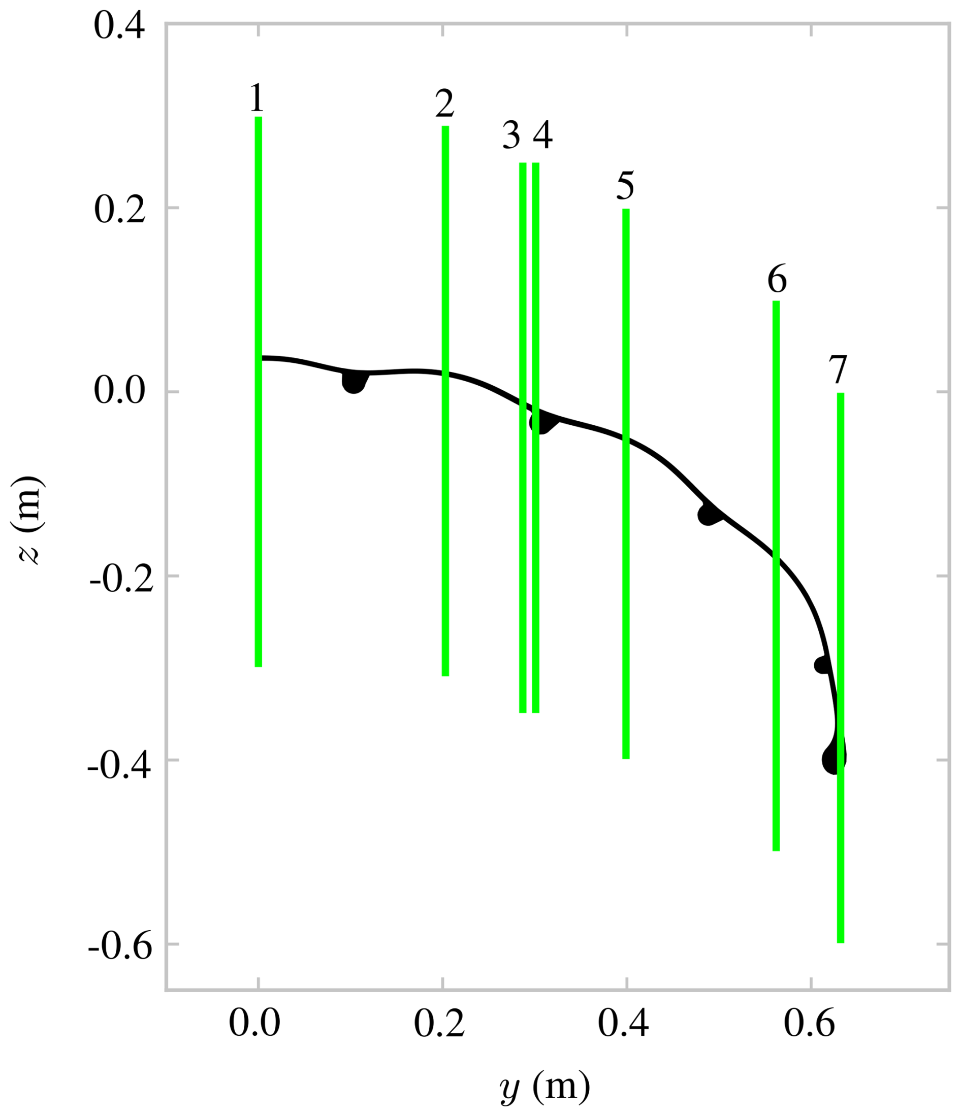
Figure 4 Arrangement of the measurement planes along the span for α = 7° at 10 % $x/c$ aft of the mid-span leading edge.

Table 3 Bottom-left corners of the measurement planes, shown in Fig. 5, at α = 0°.

2.6 Data processing

The measurements were processed using LaVision's DaVis 10 software (LaVision GmbH, 2025). The procedure consisted of the following steps:

• 1.

  averaging the image sequence;

• 2.

  normalizing each image by the computed average;

• 3.

  applying a temporal filter with a filter length of five images;

• 4.

  applying masks to exclude regions not of interest;

• 5.

  performing the PIV analysis using interrogation windows of 64 px × 64 px with two passes and 50 % overlap; and

• 6.

  averaging the resulting vectors, including only data with at least 25 source vectors and falling within 2 standard deviations of the mean – the first and second steps normalize the local light intensity to enhance particle detection, which proved to be particularly useful in regions affected by reflections.

For each measurement plane, six partially overlapping sub-planes were acquired and combined into a single field on a common grid, illustrated in Fig. 5. Each sub-plane was first shifted to a shared coordinate system and interpolated onto the common grid. Non-overlapping regions were copied directly. In overlap regions, values from the two contributing sub-planes were blended using a smooth sigmoid ramp to avoid discontinuities. Across an overlap of length L, a normalized coordinate $x\in [\mathrm{0},\mathrm{1}]$ was defined and the weight

$$\begin{array}{}\text{(3)}& w\left(x\right)={\displaystyle \frac{\mathrm{1}}{\mathrm{1}+\exp \left[-k\left(x-\frac{\mathrm{1}}{\mathrm{2}}\right)\right]}}\end{array}$$

was applied, such that the stitched value is $(\mathrm{1}-w){\mathit{\varphi }}_{\mathrm{1}}+w{\mathit{\varphi }}_{\mathrm{2}}$, where ϕ₁ and ϕ₂ denote the fields from the two sub-planes. A steepness parameter k=10 was selected empirically to balance smoothness and transition width. The same blending procedure was used for both streamwise and transverse stitching and was applied identically to all reported variables. In the remainder of the paper, the result of stitching these six measurements is referred to as a single measurement plane.

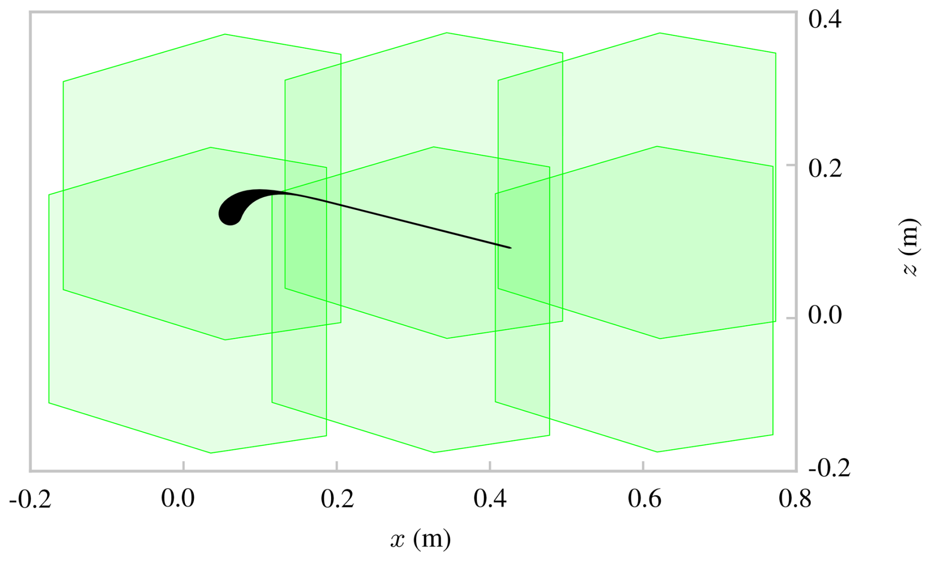
Figure 5 Mid-span cross-sectional view showing the LEI airfoil and the six overlapping measurement regions that, together, form plane Y1. The intentional overlap ensures full coverage of the flow field.

2.7 Derivation of integral aerodynamic quantities

The PIV measurements yield datasets of scalar- and vector-valued flow field properties, including the spatial coordinates x; the streamwise, lateral, and vertical components u_x, u_y, and u_z, respectively; the velocity magnitude u; and the spatial derivatives of the velocity components. From these discrete data, the components u_x and u_z are interpolated along a suitable closed planar boundary curve S around the airfoil. In the present study, this boundary is defined as a closed planar curve within a single measurement plane, such that the resulting force estimates represent sectional, pseudo-2D loads per unit span and neglect out-of-plane momentum transport. This allows for the computation of the circulation Γ as a line integral of the velocity field,

$$\begin{array}{}\text{(4)}& \mathrm{\Gamma }=\underset{S}{\oint }\mathit{u}\cdot \mathrm{d}\mathbf{s},\end{array}$$

quantifying the rotational strength of the flow in that region. Given the circulation, the 2D lift per unit span can be approximated using the Kutta–Joukowski theorem (Anderson, 2016):

$$\begin{array}{}\text{(5)}& C_{\mathrm{l},\text{Kutta}}={\displaystyle \frac{\mathrm{2}\mathrm{\Gamma }}{U_{\mathrm{\infty }}{c}_{\text{ref}}}}.\end{array}$$

This equation assumes that the integration boundary lies within the potential flow region surrounding the object of interest and that the flow is steady and attached. Nevertheless, although derived from an inviscid formulation, the circulation-based method retains theoretical validity in viscous flows, with Liu et al. (2015) proving the exact applicability of the Kutta–Joukowski relation under steady 2D viscous and compressible conditions. Because the flow is locally 3D and because Γ is evaluated from a single measurement plane, out-of-plane transport is not captured; the resulting value is therefore interpreted as an approximate sectional-lift coefficient based on U_∞ and c_ref.

The aerodynamic force on an airfoil can be obtained from the integral momentum balance over a fixed control volume V bounded by a closed surface S with outward unit normal n. For an incompressible, statistically steady flow,

$$\begin{array}{}\text{(6)}& {\mathbf{F}}_{\text{body}}=\underset{S}{\int }(-p\mathbf{n}+\mathit{\tau }\cdot \mathbf{n})\mathrm{d}S-\underset{S}{\int }\mathit{\rho }\mathbf{u}(\mathbf{u}\cdot \mathbf{n})\mathrm{d}S,\end{array}$$

where F_body denotes the net aerodynamic force on the body, p denotes the static pressure, u denotes the velocity field, and τ denotes the viscous stress tensor. In special cases, pressure contributions can be minimized by choosing a control surface that extends sufficiently far into the wake such that static pressure recovers to p_∞ and viscous traction on the outer boundary is negligible. Under these conditions, drag may be estimated from the far-wake streamwise momentum deficit, whereas lift follows from the transverse momentum balance associated with wake downwash and vorticity. In both cases, the pressure-free simplification requires a far-field control surface that encloses the full wake and lies in a region of pressure recovery. For lift in particular, accurate force recovery additionally requires that the control surface captures the spatial extent of the induced velocity field since truncation of the lateral or vertical boundaries introduces non-negligible momentum and pressure flux contributions associated with downwash and tip vortex transport.

These conditions are not satisfied for the present dataset. The available PIV measurements are confined to the near field so that any admissible control surface would necessarily intersect regions of separated flow, shear layers, and the developing wake, where static pressure has not recovered to p_∞ and contributes non-negligibly to the surface integral momentum balance. Consequently, neither drag nor lift can be obtained from a pressure-free control volume formulation without an additional pressure reconstruction step, which is not accessible from planar PIV data alone.

Moreover, as discussed in Sect. 3, near-wall velocity data are incomplete, preventing direct evaluation of the momentum flux through a closed control surface surrounding the body. Any attempt to apply the classical control volume balance would therefore require substantial modelling assumptions to reconstruct both the pressure distribution and the masked near-wall velocity field, rendering the approach ill-posed under the present experimental constraints.

Noca et al. (1999) proposed an alternative formulation of the momentum conservation equations that expresses aerodynamic forces in terms of boundary integrals involving velocity, vorticity, and their temporal and spatial derivatives. Although Noca's method involves higher-order velocity gradients and temporal derivatives that are sensitive to measurement noise, it enables a closed force formulation under the present experimental constraints. Noca's method has been successfully applied in similar PIV-based force estimation studies, including horizontal-axis wind turbines (Fritz et al., 2024a, b) and vertical-axis wind turbines (LeBlanc and Ferreira, 2022). The method, expressed in symbolic notation, evaluates the force per unit density as

$$\begin{array}{}\text{(7)}& {\displaystyle \frac{\mathit{F}}{\mathit{\rho }}}=\underset{S}{\oint }\mathit{n}\cdot {\mathit{\gamma }}_{\text{flux}}\mathrm{d}s-\underset{S_{\mathrm{b}}}{\oint }\mathit{n}\cdot (\mathit{u}-{\mathit{u}}_{\mathrm{b}})\mathit{u}\mathrm{d}s-{\displaystyle \frac{\mathrm{d}}{\mathrm{d}t}}\underset{S_{\mathrm{b}}}{\oint }\mathit{n}\cdot \left(\mathit{u}\mathit{x}\right)\mathrm{d}s,\end{array}$$

where

$$\begin{array}{}\text{(8)}& \begin{array}{rl}{\mathit{\gamma }}_{\text{flux}}=& {\displaystyle \frac{\mathrm{1}}{\mathrm{2}}}{u}^{\mathrm{2}}\mathit{I}-\mathit{u}\mathit{u}-{\displaystyle \frac{\mathrm{1}}{\mathcal{N}-\mathrm{1}}}\mathit{u}(\mathit{x}\times \mathit{\omega })+{\displaystyle \frac{\mathrm{1}}{\mathcal{N}-\mathrm{1}}}\mathit{\omega }(\mathit{x}\times \mathit{u})\\ & -{\displaystyle \frac{\mathrm{1}}{\mathcal{N}-\mathrm{1}}}\left(\mathit{x}\cdot {\displaystyle \frac{\partial \mathit{u}}{\partial t}}\right)\mathit{I}+{\displaystyle \frac{\mathrm{1}}{\mathcal{N}-\mathrm{1}}}\mathit{x}{\displaystyle \frac{\partial \mathit{u}}{\partial t}}-{\displaystyle \frac{\partial \mathit{u}}{\partial t}}\mathit{x}\\ & +{\displaystyle \frac{\mathrm{1}}{\mathcal{N}-\mathrm{1}}}[\mathit{x}\cdot (\mathbf{\nabla }\cdot \mathit{\tau }\left)\right]\mathit{I}-{\displaystyle \frac{\mathrm{1}}{\mathcal{N}-\mathrm{1}}}\mathit{x}(\mathbf{\nabla }\cdot \mathit{\tau })+\mathit{\tau },\end{array}\end{array}$$

and n is the normal vector on the bounding curve, S is the outer boundary curve of the control volume surrounding the immersed body, S_b is the inner boundary curve prescribed by the immersed body's surface, u_b is the velocity vector of the immersed body's surface, 𝒩 represents the number of dimensions, $\mathit{\omega }=\mathbf{\nabla }\times \mathit{u}$ is the flow vorticity, x is the position vector, I is the identity tensor, and τ is the viscous stress tensor. In the present pseudo-2D application, S and S_b are closed planar curves, and ds denotes arc length.

The second term on the right-hand side of Eq. (7) represents the advective momentum flux through the body boundary. For an impermeable surface, the no-throughflow condition enforces $\mathit{n}\cdot (\mathit{u}-{\mathit{u}}_{\mathrm{b}})=\mathrm{0}$ on S_b; hence, this term vanishes. The third term also vanishes for the present stationary model (u_b=0) because, on S_b, the no-throughflow condition implies $\mathit{n}\cdot \mathit{u}=\mathrm{0}$, and, therefore, $\mathit{n}\cdot \left(\mathit{u}\mathit{x}\right)=(\mathit{n}\cdot \mathit{u})\mathit{x}=\mathbf{0}$.

Equation (8) describes 10 individual contributions: the first 4, presented in the first line, are inviscid contributions; the following 3 represent unsteady terms associated with local acceleration; and the final 3 account for viscous effects. Because the present force estimates are evaluated from time-averaged, statistically steady velocity fields, the explicit time-derivative contributions in Eq. (8) vanish in the formulation adopted here. While Noca's method is inherently 3D, here, it was applied to a pseudo-2D incompressible flow problem by setting the out-of-plane velocity u_y to zero. Other out-of-plane quantities, such as the vorticity component ω_y, were retained, consistently with the pseudo-2D flow assumption. This simplification reduced the governing equations accordingly; the full derivation is provided in Appendix B. The non-zero contributions were computed directly from the discrete velocity field on the measurement grid using finite differences, based on smoothed velocity data.

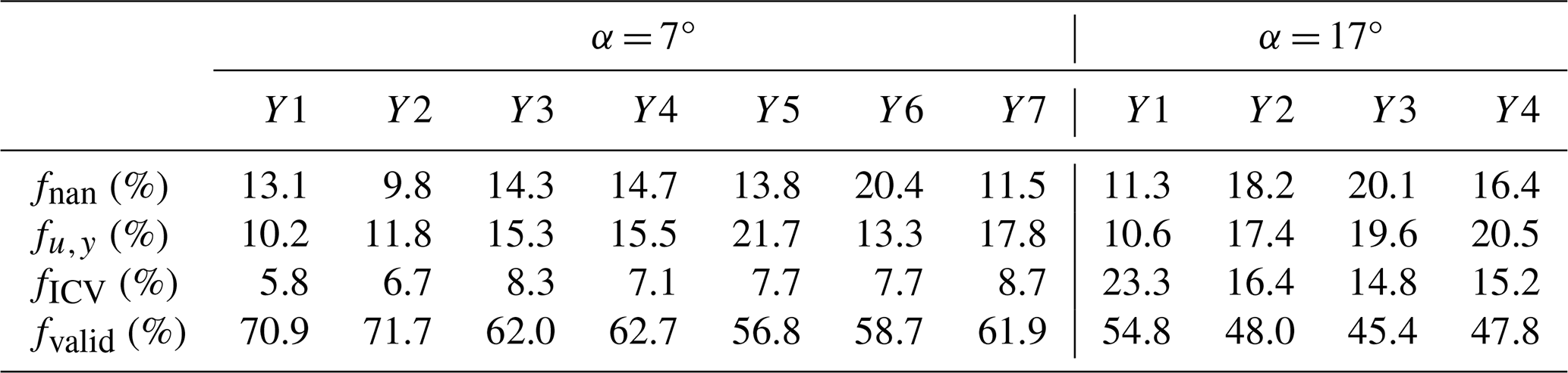
Table 4 Data quality metrics per measurement plane, showing f_nan, f_u,y, f_ICV, and the remaining valid data fraction f_valid.

Since the CFD simulations provide the flow field for the entire domain, 2D aerodynamic forces can also be derived from surface pressure and shear force integrations. Here, the integration was performed over sectional airfoil surfaces, yielding pseudo-2D aerodynamic loads directly comparable to planar PIV-based force estimates. The total aerodynamic force acting on the airfoil section is computed as

$$\begin{array}{}\text{(9)}& \mathit{F}=\underset{S_{\mathrm{b}}}{\oint }(-p\mathit{I}+\mathit{\tau })\cdot \mathit{n}\mathrm{d}s,\end{array}$$

where p is the static pressure, and τ is the viscous stress tensor.

3 Results

This section presents the results obtained from stereoscopic PIV experiments, including an uncertainty assessment, a qualitative comparison of measured and simulated velocity fields, and a quantitative analysis of circulation and aerodynamic loads.

3.1 Uncertainty analysis

Following established PIV uncertainty practice, type-A (statistical) and type-B (systematic/modelling) contributions are distinguished (Sciacchitano and Wieneke, 2016). Type-A uncertainty of the mean velocity, arising from the finite ensemble size, is quantified from the sample standard deviation and the number of samples. Systematic effects, including stereo-calibration and mapping residuals, correlation bias (peak locking), finite light-sheet thickness, masking, stitching, and measurement plane misalignment, are discussed separately.

Among the systematic (i.e. non-random, repeatable) effects, two experiment-specific artefacts dominate the present dataset. First, reflection-induced correlation failure near the surface necessitates the masking of near-wall regions. An additional diagnostic filter based on the out-of-plane velocity component, $\left|u_y\right|$ > 3 m s⁻¹, is applied to suppress stereo-reconstruction errors in these regions. The selected threshold is consistent with CFD-predicted bounds (Appendix C). It does not represent a physical constraint on three-dimensional flow but rather reflects the amplification of reconstruction errors in the out-of-plane component due to the inherent anisotropy of stereo-PIV (Sciacchitano and Wieneke, 2016).

Second, measurement plane misalignment increases towards the wing tip, enhancing out-of-plane transport and progressively reducing the validity of pseudo-2D sectional assumptions. This effect contributes to increased data loss and reduced reliability of near-wall velocity information in the outboard planes.

To suppress residual temporally incoherent velocity vectors, an additional filter based on the inverse coefficient of variation (ICV) is applied. For each grid point i, the ICV is defined as

$$\begin{array}{}\text{(10)}& \text{ICV}\left(i\right)=\text{median}\left({\displaystyle \frac{\left|\stackrel{\mathrm{‾}}{u_x}\right(i\left)\right|}{{\mathit{\sigma }}_{u_x}\left(i\right)}},{\displaystyle \frac{\left|\stackrel{\mathrm{‾}}{u_z}\right(i\left)\right|}{{\mathit{\sigma }}_{u_z}\left(i\right)}}\right),\end{array}$$

where $\stackrel{\mathrm{‾}}{(\cdot )}$ and σ_(⋅) denote the ensemble mean and standard deviation. Low ICV values indicate unreliable velocity estimates associated with correlation failure. To avoid the suppression of physically unsteady flow regions, the filter is spatially restricted to the near-surface reflection-prone region. Further implementation details are provided in Appendix C.

The impact of these quality control steps on data availability is summarized in Table 4. The fraction f_nan denotes vectors rejected during correlation and validation and primarily reflects reflection- and geometry-induced loss of correlation. The fraction $f_{u_y}$ represents additional rejection due to the out-of-plane velocity filter, and f_ICV denotes vectors removed by the ICV-based filter. These quantities describe data availability rather than measurement uncertainty; their impact arises through increased interpolation and reduced spatial coverage.

The reduction in usable data arises from multiple filtering steps of comparable magnitude. The out-of-plane velocity filter contributes 6 %–13 % data loss, increasing towards the wing tip due to enhanced three-dimensional flow effects and measurement plane misalignment. The ICV filter contributes 5 %–9 % data loss at α = 7°, increasing to 15 %–23 % at α = 17°, consistently with increased flow unsteadiness and degraded correlation quality.

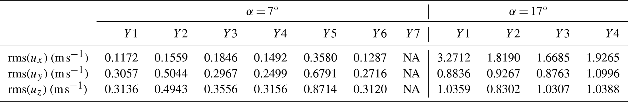
Table 5 Expanded uncertainties of the mean velocity corresponding to a 95 % confidence interval (k≈ 1.960), calculated from N=250 samples and aggregated over all data points within a measurement plane. These values quantify statistical convergence only and do not include systematic (type-B) contributions.

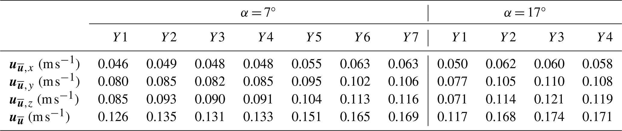
Despite these reductions, the sample size is sufficient to ensure convergence of the time-averaged velocity statistics, as demonstrated in Appendix A. The type-A uncertainty of the mean velocity is quantified as

$$\begin{array}{}\text{(11)}& u_{\stackrel{\mathrm{‾}}{u}}=k{\displaystyle \frac{{\mathit{\sigma }}_{\mathrm{u}}}{\sqrt{N}}},\end{array}$$

where σ_u is the sample standard deviation, N is the number of image pairs, and k is the coverage factor corresponding to a 95 % confidence interval. Temporal correlation between successive image pairs is not explicitly accounted for; if present, it reduces the effective sample size and leads to a mild underestimation of the type-A uncertainty.

Table 5 summarizes $u\stackrel{\mathrm{‾}}{u}$ for each velocity component, obtained by evaluating the sample standard deviation over N=250 image pairs at each grid point and aggregating the result per measurement plane. The uncertainty levels increase towards the wing tip, consistently with increased measurement plane misalignment and surface reflections. At α = 17°, uncertainties are higher due to increased flow unsteadiness and intermittency. Relative to the inflow velocity U_∞ = 15 m s⁻¹, the expanded uncertainties correspond to approximately 0.8 %–1.2 %. These values define the baseline accuracy for subsequent velocity field comparisons and represent the lower bound for detectable discrepancies between PIV and CFD.

In addition to the statistical (type-A) uncertainty, discrepancies arise from the stitching of partially overlapping PIV sub-planes. The magnitude of residual velocity differences across overlap regions is quantified independently in Appendix D. This metric does not represent a formal uncertainty estimate but provides a local measure of consistency between independently acquired sub-planes at identical spatial locations.

3.2 Comparing flow fields

The measured velocity fields are compared against corresponding slices from CFD simulations by Viré et al. (2022), extracted at the same locations. The CFD results presented here have been corrected for a 1.02° offset in angle of attack, defined as the angle between the mid-span chord line and the apparent wind vector (Poland et al., 2026b). This constant offset accounts for a difference in α definition and zero reference between the CFD and the experiment, whereas the streamline curvature correction in Table 1 is applied to the experimental angles to account for wind tunnel interference effects. CFD results, available only at Re = 10 × 10⁵ with struts, are compared against measurements conducted at 3.8 × 10⁵.

Analysis of integral 3D forces and moments from the companion study (Poland et al., 2026b) showed an approximate 6 % difference in lift between Re = 3.8 × 10⁵ and Re = 6.1 × 10⁵ at α = 7.4°, confirming Reynolds number sensitivity within the experimentally accessible range. RANS simulations (Viré et al., 2022) further indicate that increasing Re leads to higher C_L. However, simulations without struts show little sensitivity between Re = 5 × 10⁵ and higher-Re cases (Viré et al., 2020; Poland et al., 2026b), whereas CFD with struts at Re = 1 × 10⁵ exhibit a measurable offset relative to Re = 5 × 10⁵ and Re = 10 × 10⁵, suggesting increased sensitivity at lower Reynolds numbers. Since the CFD reference is at Re = 10 × 10⁵, some deviation from the measurements at Re = 3.8 × 10⁵ is expected, most likely in the form of reduced lift, although the precise magnitude of this effect remains unresolved.

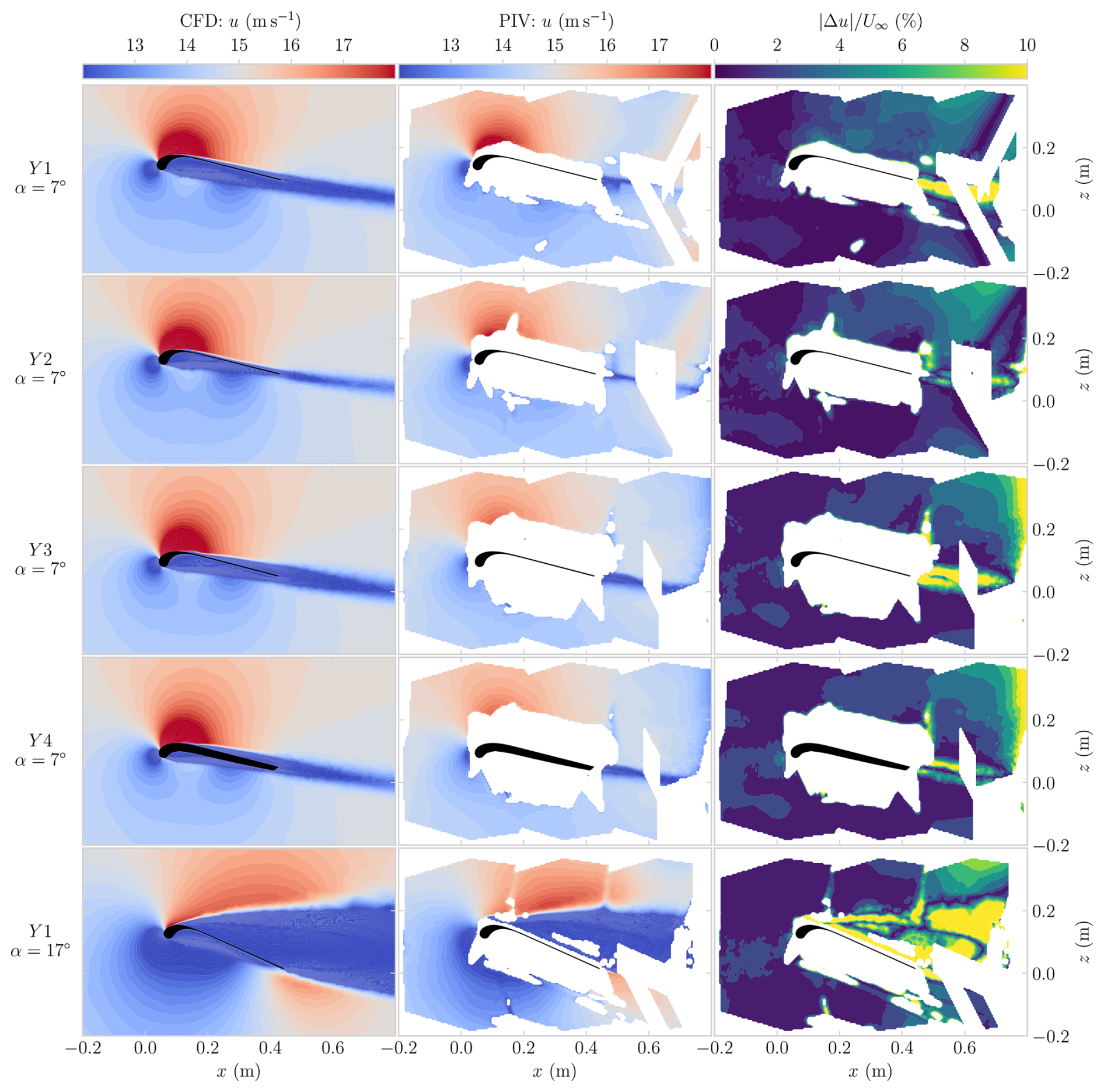
Figure 6 Comparison of CFD-predicted and PIV-measured velocity–magnitude fields u. The first column shows CFD slices extracted at the measurement plane locations, and the second column shows the corresponding PIV results. Rows (top to bottom) show planes Y1, Y2, Y3, and Y4 at α = 7° and plane Y1 at α = 17°. In the third column, the absolute differences between CFD and PIV are shown as a percentage of U_∞.

Velocity magnitude fields for the measurement planes are presented in Fig. 6 for sections Y1, Y2, Y3, and Y4 at α = 7°, and for Y1 at α = 17°. This subset is selected for qualitative comparison because these planes exhibit a combination of lower stitching uncertainty (Appendix D) and higher f_valid, as reported in Table 4. The absolute velocity difference, normalized by the mean inflow velocity U_∞, is shown to emphasize both local discrepancies and the overall level of agreement.

No PIV data are available in the immediate vicinity of the airfoil surface because near-wall regions are masked owing to surface reflections and correlation loss. An exception occurs on the suction side of the α = 17° cases, where the ICV mask is spatially restricted to preserve the separation zone. As a result, only CFD captures the expected separated-flow region downstream of the leading-edge tube. The masked region expands progressively from Y1 to Y4, which is consistent with increasing surface reflection severity and growing measurement plane misalignment towards the wing tip.

Among the six stitched measurements, the top-right panel exhibits deviations near the domain edge. A second deviation region (yellow) arises from wake interactions, most clearly observed in Y1 and Y3 at α = 7° and in Y1 at α = 17°. For the majority of the flow field, however, the PIV measurements and CFD predictions agree within 5 %.

Qualitatively, the contour topology is consistent between both datasets, with suction peaks indicated by locally increased velocities and pressure regions by reduced velocity contours. Even at α = 17°, both datasets resolve the key flow features: suction-side separation, a diminished velocity increase on the suction side, shear layer development, and the associated velocity gradients. These features are consistent with the anticipated stall behaviour inferred from the integral force measurements (Poland et al., 2026a).

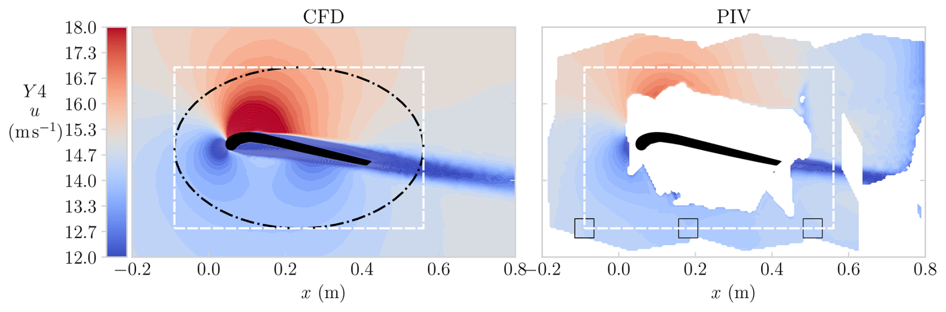
Figure 7 The velocity magnitude field, u, is shown for both CFD (left) and PIV (right) at plane Y4 and angle of attack α = 7°. In the CFD field, both elliptical and rectangular boundary curves are indicated. In the PIV field, a rectangular boundary curve is shown together with black-square markers denoting locations where interpolation of the velocity field was required to populate the contour nodes.

3.3 Boundary curve selection

Aerodynamic properties were obtained by integrating the velocity field along parameterized boundary curves enclosing the lifting surface. Two curve geometries, elliptical and rectangular, were considered, as illustrated in Fig. 7. Each curve is defined by its centre location, rotation angle, width, height, and boundary node discretization. When a boundary intersected regions with missing data, the velocity field was locally reconstructed using a distance-weighted interpolation and was subsequently sampled at the boundary nodes by linear interpolation, with nearest-neighbour fallback outside the convex hull. Missing vectors within contour-adjacent square regions were reconstructed using a distance-weighted interpolation, after which contour node values were obtained by linear scattered interpolation, with nearest-neighbour fallback outside the convex hull.

To assess sensitivity to the integration contour, the nominal curve dimensions were perturbed by ±5 % in width and height, generating an ensemble of 36 contour realizations per geometry. Circulation was evaluated for each realization, and ensemble-averaged results are reported. Further details on contour convergence and the selection of nominal dimensions are provided in Appendix E.

To ensure that contour-based evaluations remain representative of the measured flow field, an admissibility criterion was imposed based on data availability along the boundary. Contours for which more than 20 % of the interpolation region points required reconstruction from initially missing data were excluded from the analysis. This threshold limits the influence of interpolation-dominated regions and ensures that the reported circulation and force estimates are primarily supported by measured velocity data.

3.4 Circulation distribution

The spanwise distributions of circulation strength Γ obtained from CFD and PIV are shown in Fig. 8. VSM predictions at Re = 3.8 × 10⁵, computed using the recommended settings and 2D polars from the companion paper (Poland et al., 2026a), are included for comparison. The PIV results are reported up to plane Y6 since plane Y7 required excessive interpolation, exceeding 20 % of the required interpolation region points. For CFD, plane Y7 was also left out as the predicted value was an order of magnitude off and showed large uncertainty, attributed to the plane misalignment. Circulation is reported only for α = 7° because the uncertainty levels at α = 17° were too large at planes Y2–Y4 (Appendix D).

Figure 8 The circulation distribution at α = 7°, computed using boundary curve velocity interpolation, is shown for CFD across all measurement planes, for PIV data up to plane Y6, and as predicted by the VSM method. The distributions are overlaid on the wing outline, with the measurement plane locations indicated; these are not shown to scale.

The intervals shown in Fig. 8 quantify the sensitivity of the circulation strength Γ to the integration contour. For each contour geometry, Γ was evaluated over an ensemble of perturbed contours, and the reported value corresponds to the mean of the elliptical and rectangular shape-averaged estimates. The plotted intervals represent the full min–max range across the contour ensemble for each dataset, thereby isolating contour sensitivity rather than total measurement uncertainty.

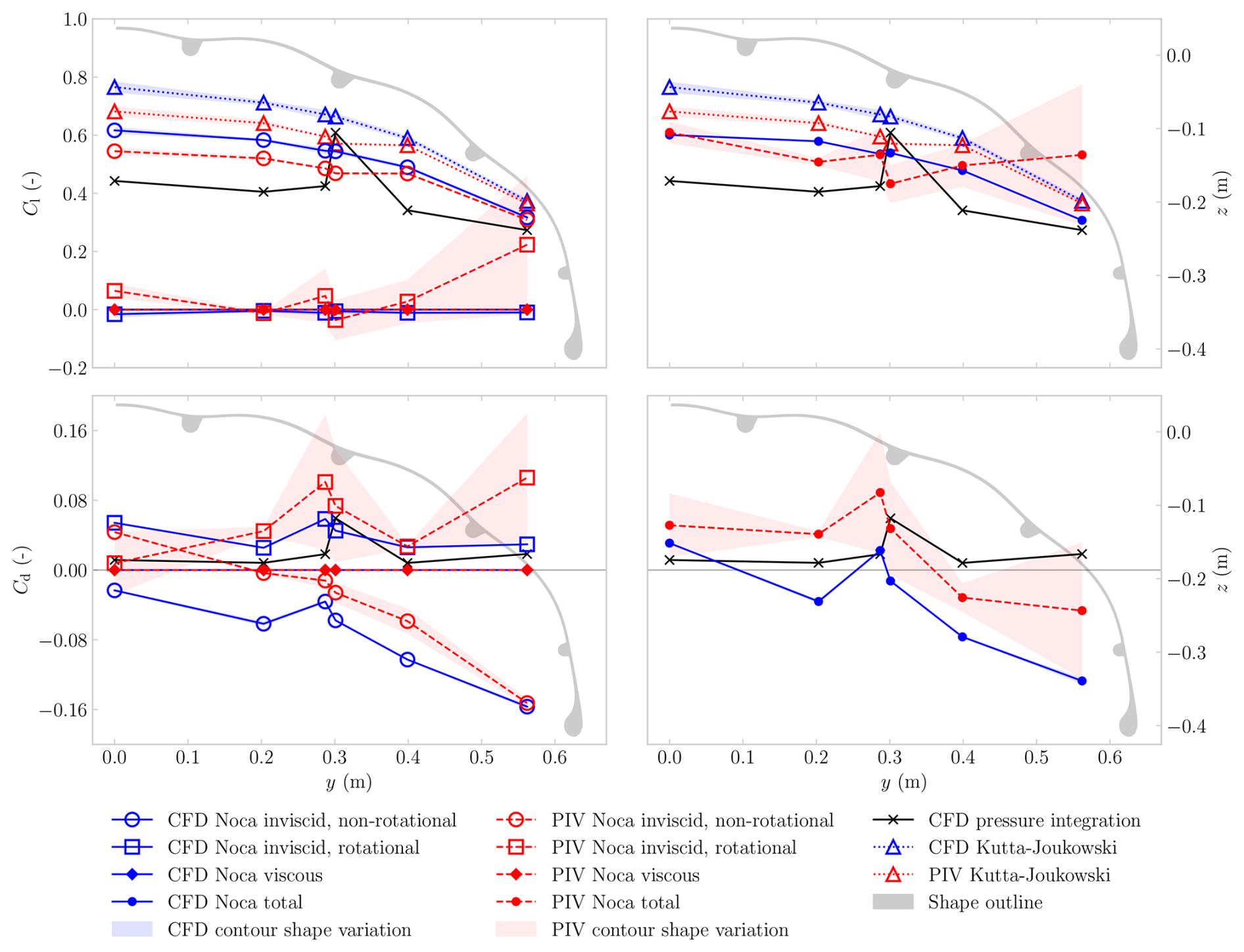
Figure 9 Spanwise distributions of sectional force coefficients at α = 7° from CFD and PIV. The upper row shows C_l, and the lower row shows C_d. The left column compares the individual Noca contributions, namely the inviscid, non-rotational, inviscid, rotational, and viscous terms, with the pressure integration and Kutta–Joukowski predictions. The right column compares the total Noca, the pressure integration, and the Kutta–Joukowski results.

The CFD-derived Γ distributions exhibit a narrow spread, indicating that the results are only weakly sensitive to contour geometry, with further convergence towards the wing tip. The PIV-derived distributions follow a similar spanwise trend but are approximately 10 %–15 % lower inboard, with the discrepancy decreasing towards the tip. The lower observed values are consistent with potential Reynolds-number-induced differences between the higher-Re CFD and the lower-Re experimental conditions, which were hypothesized to lead to increased lift in the CFD. The largest deviation occurs at Y4, where the measurement plane intersects a strut, as further discussed in Sect. 4.2.

The comparatively small spread of the PIV ensemble in the outboard planes is partly a methodological artefact. Extensive missing data reduce the number of admissible contour realizations, thereby artificially narrowing the ensemble variability. This effect is most pronounced at Y6, as illustrated in Fig. D1.

Despite differences in numerical formulation, the RANS-based CFD and VSM predictions, along with the PIV-measured distributions, exhibit similar spanwise trends and comparable magnitudes of circulation. This overall agreement may contribute to the consistency of the integration routine and indicates that both the numerical models and the measurements capture the spanwise distribution of aerodynamic loading. It also reduces the likelihood that the previously reported agreement in integral lift (Poland et al., 2026a) arises from compensating errors.

3.5 Planar forces

To compare force estimates from circulation- and velocity-based approaches, sectional aerodynamic forces are evaluated using the Kutta–Joukowski theorem, the Noca formulation, and pressure integration. The resulting spanwise distributions for α = 7° are shown in Fig. 9. The corresponding values are listed in Table F1 in Appendix F, which also includes results for the Y1 plane at α = 17°. The Y7 plane is excluded because its excessive misalignment renders the force estimates unreliable.

To interpret the contributions of individual terms in the Noca formulation, the equation is decomposed into the following: inviscid non-rotational, inviscid rotational, and viscous components.

The inviscid non-rotational contribution is

$$\begin{array}{}\text{(12)}& {\displaystyle \frac{{\mathit{F}}_{\text{inv},\text{nonrot}}}{\mathit{\rho }}}=\underset{S}{\oint }\mathit{n}\cdot \left({\displaystyle \frac{\mathrm{1}}{\mathrm{2}}}{u}^{\mathrm{2}}\mathbf{I}-\mathit{u}\mathit{u}\right)\mathrm{d}s.\end{array}$$

The inviscid rotational contribution is

$$\begin{array}{}\text{(13)}& \begin{array}{rl}{\displaystyle \frac{{\mathit{F}}_{\mathrm{inv},\mathrm{rot}}}{\mathit{\rho }}}=& \underset{S}{\oint }\mathit{n}\cdot \left(-{\displaystyle \frac{\mathrm{1}}{\mathcal{N}-\mathrm{1}}}\mathit{u}(\mathit{x}\times \mathit{\omega })\right.\\ & \left.+{\displaystyle \frac{\mathrm{1}}{\mathcal{N}-\mathrm{1}}}\mathit{\omega }(\mathit{x}\times \mathit{u})\right)\mathrm{d}s.\end{array}\end{array}$$

The viscous contribution is

$$\begin{array}{}\text{(14)}& \begin{array}{rl}{\displaystyle \frac{{\mathit{F}}_{\mathrm{visc}}}{\mathit{\rho }}}=& \underset{S}{\oint }\mathit{n}\cdot \left({\displaystyle \frac{\mathrm{1}}{\mathcal{N}-\mathrm{1}}}\left[\mathit{x}\cdot (\mathbf{\nabla }\cdot \mathit{\tau })\right]\mathbf{I}\right.\\ & \left.-{\displaystyle \frac{\mathrm{1}}{\mathcal{N}-\mathrm{1}}}\mathit{x}(\mathbf{\nabla }\cdot \mathit{\tau })+\mathit{\tau }\right)\mathrm{d}s.\end{array}\end{array}$$

For C_l, retaining only the inviscid, non-rotational terms yields the most consistent estimates in terms of both magnitude and spanwise trend. For this contribution, the CFD- and PIV-derived Noca estimates agree within 10 %–15 % and exhibit the expected monotonic decrease in C_l, consistently with the behaviour observed for Γ. As with Γ, part of the lower magnitude may be attributed to the lower Re of the PIV measurements. Including all terms (Noca total) has only a minor effect on CFD but introduces a substantial deviation in PIV. This discrepancy originates from the inviscid, rotational terms as the viscous contribution to C_l is negligible.

For C_d, the dominant contributions are reversed relative to C_l. Retaining only the inviscid, rotational terms yields the most physically consistent results as the inviscid, non-rotational terms produce unphysical negative drag values for both CFD and PIV. Viscous contributions remain negligible throughout. For these terms, the PIV- and CFD-derived Noca estimates align with the CFD pressure-integration-predicted drag increases around the strut (near y=0.3m).

Two competing effects govern the spanwise evolution of the contour spread in the Noca force integral. Increased data masking towards the wing tip requires greater interpolation, which raises sensitivity to contour geometry and tends to increase the ensemble spread. At the same time, the admissibility threshold of 20 % for interpolation region points reduces the number of admissible contour realizations, introducing a selection bias that reduces the observable variability.

These mechanisms affect the individual contributions differently. The inviscid, rotational contribution depends on the spatial distribution of rotational-flow structures relative to the integration contour and is therefore sensitive to vortex position and to interpolation-induced noise as vorticity is derived from velocity gradients. These sensitivities intensify towards the wing tip, increasing its spread. Conversely, the inviscid, non-rotational contribution depends directly on the velocity field itself rather than on its spatial gradients and is therefore comparatively insensitive to the precise position of concentrated vortical structures. Consequently, it does not exhibit the same tip-ward increase in ensemble spread.

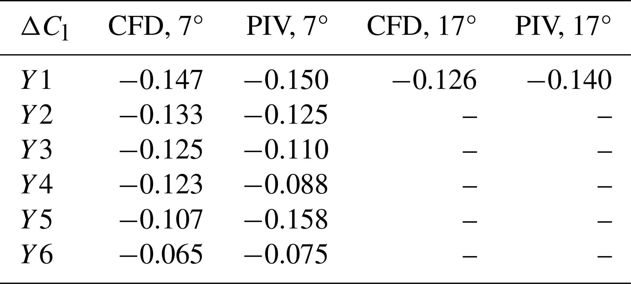
The Kutta–Joukowski estimate of C_l exhibits a consistent spanwise trend, supporting the internal coherence of the force reconstruction, but yields systematically higher magnitudes. This difference is consistent with the present near-field formulation and does not contradict the Noca estimate as the two are equivalent only in the ideal far-field limit of steady, strictly two-dimensional, irrotational flow. This can be illustrated by expressing the inviscid, non-rotational Noca lift as the sum of a Kutta–Joukowski term and a finite-contour correction:

$$\begin{array}{}\text{(15)}& \begin{array}{rl}{\displaystyle \frac{F_{z,\text{inv},\text{nonrot}}}{\mathit{\rho }}}& =\underset{S}{\oint }\left[{\displaystyle \frac{\mathrm{1}}{\mathrm{2}}}{n}_z\left(u_x^{\mathrm{2}}-u_z^{\mathrm{2}}\right)-n_x{u}_x{u}_z\right]\mathrm{d}s\\ & =U_{\mathrm{\infty }}\mathrm{\Gamma }+\underset{S}{\oint }\left[{\displaystyle \frac{\mathrm{1}}{\mathrm{2}}}{n}_z\left({\stackrel{\mathrm{̃}}{u}}_x^{\mathrm{2}}-{\stackrel{\mathrm{̃}}{u}}_z^{\mathrm{2}}\right)-n_x{\stackrel{\mathrm{̃}}{u}}_x{\stackrel{\mathrm{̃}}{u}}_z\right]\mathrm{d}s,\end{array}\end{array}$$

where $\stackrel{\mathrm{̃}}{\mathit{u}}=\mathit{u}-U_{\mathrm{\infty }}{\mathbf{e}}_x$ is the perturbation velocity. The second integral is a quadratic correction that vanishes only in the ideal limit and was found to be negative for all planes in the present analysis (Table F2 in Appendix F), thereby explaining the higher lift magnitudes predicted by the Kutta–Joukowski formulation compared to the Noca estimate.

Comparison with CFD pressure integration provides an independent reference based on the complete CFD solution. Consistently with the observed trends and the requirement of positive drag values, the closest agreement is obtained for C_l when retaining only the inviscid, non-rotational terms and for C_d when retaining only the inviscid, rotational terms. The systematically lower C_l magnitudes from pressure integration are attributed to contour-based methods that sample a comparatively larger near-field region, where three-dimensional induced velocities increase the apparent momentum flux relative to the force inferred from local surface pressure. The surface pressure integral is also affected by three-dimensional flow but is less sensitive as it depends only on wall conditions rather than integrating over the surrounding flow field.

Overall, while both the Noca method and the Kutta–Joukowski theorem predict a near-monotonic spanwise decrease in lift from Y1 to Y6, the pressure integration results deviate from this trend at planes Y3 and Y4, exhibiting a local increase in both lift and drag, most pronounced at Y4. Unlike the distributed three-dimensional effects discussed above, this deviation is attributed to a localized disturbance associated with the second strut, which violates the pseudo-two-dimensional assumptions underlying planar sectional analysis and is not adequately captured by planar boundary-curve-based methods. This hypothesis is examined in Sect. 4.2.

For the present near-field PIV configuration, the inviscid, non-rotational Noca contribution provides the most reliable sectional-lift estimates, whereas, for drag, the inviscid, rotational contribution yields the most physically consistent results, albeit with reduced quantitative reliability, as reflected by its larger contour-induced spread.

4 Discussion

The experimental results highlight the combined influence of measurement limitations, methodological assumptions, and local three-dimensional flow effects on the accuracy and interpretation of planar force estimates.

4.1 Measurement limitations and quantitative discrepancies

The dominant measurement limitation arises from surface reflections associated with the complex LEI wing geometry, characterized by pronounced anhedral curvature, a near-cylindrical leading edge, and multiple strut elements. Despite mitigation measures, including matte black surface treatment and tailored post-processing, reflection-induced correlation failure persists. This necessitates the masking of near-wall regions and interpolation across data gaps in the evaluation of boundary curve integrals, introducing uncertainty that is further amplified by sensitivity to the integration contour definition, as demonstrated in Appendix E.

Towards the wing tip, increasing geometric curvature causes progressive misalignment between the measurement plane and the local flow direction, amplifying out-of-plane transport and further reducing the validity of pseudo-2D sectional assumptions. These two effects – near-wall data loss and tip-ward misalignment – jointly govern the reliability of the quantitative results and explain the spanwise degradation in force estimate quality observed in Sect. 3.

Their impact differs across force components. Lift, governed primarily by large-scale momentum flux, is comparatively robust, with PIV- and CFD-derived estimates agreeing within 10 %–15 % at mid-span. In contrast, drag is inherently more sensitive as it depends on small momentum deficits and viscous contributions in the near and far wake, which are difficult to resolve accurately under the present conditions of wake truncation, masking, and incomplete near-wall data (Huang et al., 2023). This behaviour is consistent with the velocity comparison in Fig. 6, where the largest discrepancies between PIV and CFD occur in the wake region. Out-of-plane effects further amplify this sensitivity, disproportionately affecting drag relative to lift in velocity-only formulations (LeBlanc and Ferreira, 2022).

Surface pressure integration from CFD provides an independent reference that is free from the above measurement limitations. It exhibits similar spanwise trends compared to the contour-based estimates but deviates locally at planes Y3 and Y4, consistently with the strut-induced three-dimensional disturbances examined in Sect. 4.2.

The observed discrepancies arise primarily from reflection-induced data loss, which necessitates masking and interpolation and thereby introduces sensitivity into the integration contour definition. Together, these measurement and methodological effects constitute the dominant source of quantitative uncertainty in the present dataset.

4.2 Local strut effects

The following analysis addresses the off-trend sectional loads observed at planes Y3 and Y4, which coincide with the second strut location and are not reproduced by velocity-based methods. Because near-wall PIV data in the strut vicinity are insufficient to resolve the associated 3D flow, CFD results are used here solely to interpret the physical origin of these deviations.

In the literature, CFD simulations have been performed both with struts (Viré et al., 2022) and without (Viré et al., 2020). Based on comparisons of global aerodynamic properties, it was concluded that the presence of struts has little influence on overall performance. However, Viré et al. (2022) noted that struts do affect the local flow field, including increased vortex shedding. This observation was supported by spanwise plots of the λ₂ criterion, which provides an indication of vortex core lines in (Jeong and Hussain, 1995). For the case α = 13° at Re = 30 × 10⁵, developing vorticity was found on the pressure side, with structures present between $x/c=\mathrm{0.3}$ and $x/c=\mathrm{0.6}$, except near the tip vortex and the strut regions – indicative of strut-induced effects. The work of Viré et al. (2022) is the published version of the MSc thesis by Lebesque (2020), which further reported that strut blockage influenced the location and size of recirculation regions and, more generally, introduced stronger local effects.

To investigate the mechanism behind the strut-induced effect, measurement planes Y3 and Y4 were positioned at the location of the second strut. While the flow fields are not resolved close enough to the surface to investigate this mechanism using PIV, CFD results do provide sufficient resolution. As shown in Appendix C in Fig. C1, the struts do indeed appear to affect the local spanwise flow, evidenced by localized regions of increased and decreased u_y values, indicative of a strut-induced velocity increase. This interaction does not produce a uniform effect along the streamwise direction but develops progressively, particularly within the recirculation zone of the leading-edge tube.

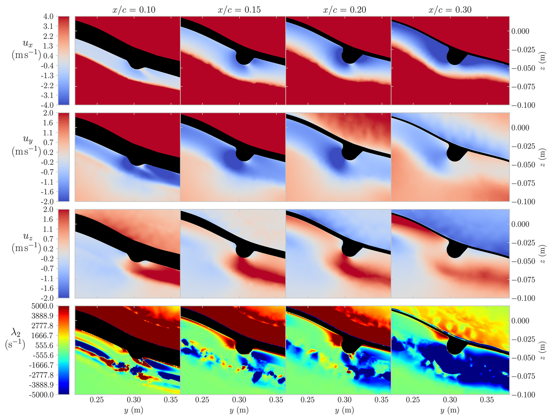
Figure 10 Spanwise CFD slices at α = 7° and Re = 10 × 10⁵ near the second strut. Columns show 4 $x/c$ locations; rows show u_x, u_y, u_z, and λ₂. Upstream slices intersect the leading-edge tube and fillet, and so the membrane is only visible at the most downstream location.

To investigate this effect, four spanwise slices focused on the second strut, ranging from $x/c=\mathrm{0.1}$ to 0.3, are shown in Fig. 10. The first row displays the streamwise velocity u, where regions of increased upstream flow around the strut are indicated by blue contours. This corresponds to an increase in downward velocity u_z, also shown in blue in the second row, and enhanced spanwise velocity u_y, shown in red in the third row. Similarly to the u component, the velocity differences in u_y and u_z become less pronounced downstream, as evident in the last column. Near the strut, the flow accelerated downward, spanwise, and upstream. This combined signature was consistent with a tilted vortex structure.

To investigate whether vortices are present, the λ₂ criterion is plotted in the last row. It is derived from the eigenvalues of the symmetric tensor E²+W², where the square denotes a matrix multiplication yielding another second-order tensor. The symmetric strain rate and antisymmetric spin tensors are defined as

$$\begin{array}{}\text{(16)}& {\displaystyle }\mathbf{E}& {\displaystyle }={\displaystyle \frac{\mathrm{1}}{\mathrm{2}}}\left(\mathrm{\nabla }\mathbf{u}+(\mathrm{\nabla }\mathbf{u}{)}^{\mathsf{T}}\right),\text{ and}\text{(17)}& {\displaystyle }\mathbf{W}& {\displaystyle }={\displaystyle \frac{\mathrm{1}}{\mathrm{2}}}\left(\mathrm{\nabla }\mathbf{u}-(\mathrm{\nabla }\mathbf{u}{)}^{\mathsf{T}}\right),\end{array}$$

respectively, where ∇u denotes the velocity gradient tensor.

The λ₂ criterion specifically evaluates the second-largest eigenvalue of this tensor, where λ₂<0 indicates the presence of a vortex core (Jeong and Hussain, 1995). The values reported here differ in magnitude from those in Viré et al. (2022) due to the adjustment in angle of attack, scaling to the projected frontal area rather than the projected side area, and the omission of the sign inversion applied in that study.

At $x/c=\mathrm{0.1}$, the λ₂ criterion indicates negative regions within the shear layer and close to the surface on the outward side of the strut. The latter region somewhat corresponds to areas of elevated u_y and u_z velocities. Closer to the strut, the shear layer structures begin to break down. The breakdown phenomenon intensifies downstream and coincides with a shear layer bulge, most clearly observed in the u-velocity field and associated with regions of negative u_y. An additional factor contributing to the downstream breakdown of the structure is enhanced turbulent mixing. By $x/c=\mathrm{0.3}$, a region of negative λ₂ values has grown in size and now covers nearly the entire recirculation region.

In summary, the strut is associated with local increases in velocity in all three spatial directions, consistently with a strong 3D interaction. This effect cannot be attributed solely to spanwise transport as elevated upstream velocities in the u direction are also observed in the strut region. The combined signatures are consistent with a 3D mechanism, such as an inclined vortex originating near the inward side of the strut, which could account for the local upstream flow. Although the upstream shear layer is clearly identified in the λ₂ field, the existence and topology of such a vortex cannot be confirmed unambiguously from the present evidence.

Nevertheless, the strut's influence on both velocity and vorticity shedding is apparent. Given the spatial overlap between these disturbed flow regions and planes Y3 and Y4, the strut effect is a credible contributor to the elevated lift and drag observed in the surface pressure integration. While global aerodynamic coefficients remain largely unaffected by strut inclusion, as reported by Viré et al. (2022), this CFD analysis demonstrates how the struts affect local aerodynamic phenomena, highlighting important implications for both experimental interpretation and sectional load modelling.

5 Conclusion

This study presents the first geometry-consistent, spatially resolved stereoscopic PIV dataset for a strongly anhedral LEI kite wing, obtained from a rigid 1:6.5 scale model of the TU Delft V3 kite under controlled wind tunnel conditions.

The measured PIV velocity fields agree with the CFD predictions to within 5 % of the freestream velocity U_∞ across the majority of the flow field, supporting the conclusion that RANS captures the dominant mean flow topology. Circulation distributions obtained from contour integration exhibit consistent spanwise trends across PIV, CFD, and VSM. The PIV values are approximately 10 %–15 % lower inboard, consistently with the lower experimental Reynolds number, and converge towards the tip.

A key finding concerns the reliability of planar force reconstruction. The inviscid, non-rotational Noca contribution provides the most consistent sectional-lift estimates, with agreement within 10 %–15 % of the CFD results at mid-span, whereas Kutta–Joukowski reproduces the spanwise trend but systematically overpredicts the magnitude. This discrepancy is attributed to a finite-contour correction inherent to the near-field formulation, which vanishes only in the ideal far-field limit. Drag recovery from near-field PIV was found to be unreliable in the present configuration: only the inviscid, rotational Noca contribution yielded physically consistent drag estimates, whereas the full formulation produces non-physical negative values. These findings indicate that, in the present case, the selective use of individual Noca contributions leads to a more physically consistent result than the direct application of the full formulation.

Another finding concerns the discrepancy between CFD surface pressure integration and contour-based planar methods in the vicinity of the strut. This difference is attributed to local, strut-induced three-dimensional flow effects: although strut effects have been shown numerically to exert negligible influence on global aerodynamic coefficients, the CFD results reveal a concentrated vortical structure near the strut junction, which locally increases sectional lift and drag relative to adjacent spanwise planes.

Despite these limitations, the dataset provides a valuable, albeit not definitive, flow-resolved validation reference for aerodynamic models of LEI kites. The consistent agreement in spanwise circulation, lift, and mean flow topology between PIV measurements and CFD predictions, across multiple approaches, supports the physical fidelity of the numerical predictions within the resolved measurement domain. Future work should focus on volumetric measurement techniques to capture out-of-plane transport, alongside improved surface treatment and acquisition strategies to mitigate reflections and recover near-wall flow.

Appendix A: Convergence over the 250 image samples

This appendix assesses whether the ensemble size of N=250 image pairs is sufficient to obtain statistically converged time-averaged velocities. A representative high-variance case was selected by considering plane Y4 at α = 17°, which exhibits the largest expanded type-A uncertainties of the mean among the retained datasets (Table 5). Time series of the instantaneous velocity components u_x, u_y, and u_z at a fixed grid point are shown in Fig. A1. To avoid visual misinterpretation associated with acquisition order, the N=250 samples were randomly permuted prior to plotting.

The monitored point is located above the airfoil surface and corresponds to image plane coordinates x = −0.75 mm and z = −118.18 mm, i.e. approximately x≈ 0.25 m and z≈ 0.25 m in the reference frame used throughout the paper (see Fig. 6). The observed fluctuations remain bounded about a stable mean without systematic drift, indicating that the time-averaged velocity estimate at this location is statistically converged for N=250 samples. Accordingly, the uncertainty metric in Eq. (11) is interpreted as a type-A (precision) uncertainty of the mean due to finite ensemble size rather than as evidence of unresolved non-stationarity.

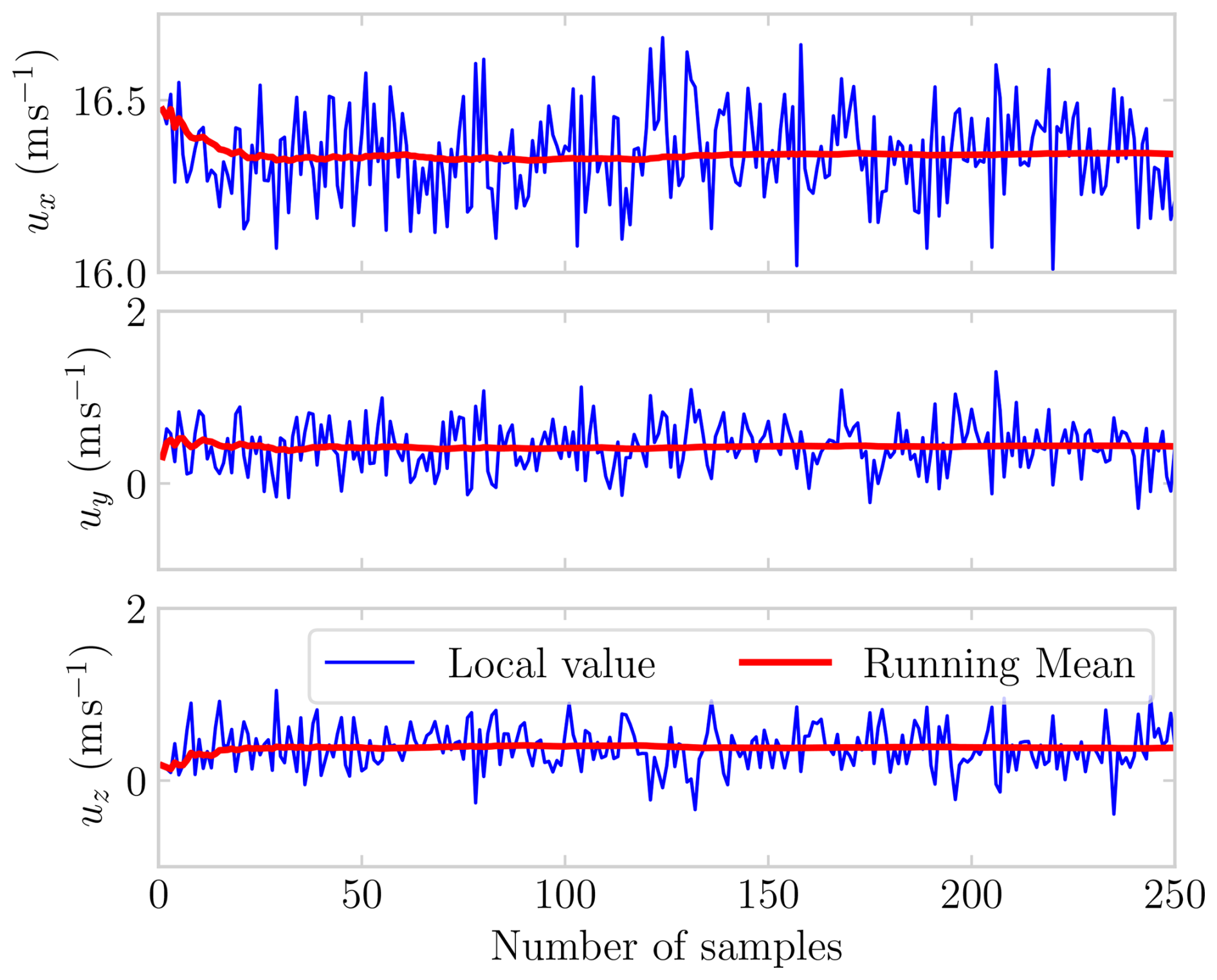
Figure A1 Instantaneous velocity components u_x, u_y, and u_z at a fixed point above the airfoil surface in plane Y4 at α = 17°. The N=250 samples are randomly permuted for visualization.

Appendix B: Noca's method, in reduced form

Noca et al. (1999) presented a 3D method for the computation of forces from a boundary surface, given sufficient flow field information. In the present work, this method was applied under the assumption of 2D incompressible flow. To reduce the dimensions 𝒩 from 3 to 2, a zero was substituted in the second component of the normal vector,

$$\begin{array}{}\text{(B1)}& \mathit{n}={\left[\begin{array}{ccc}{n}_x& \mathrm{0}& n_z\end{array}\right]}^{\top };\end{array}$$

the position vector,

$$\begin{array}{}\text{(B2)}& \mathit{x}={\left[\begin{array}{ccc}x& \mathrm{0}& z\end{array}\right]}^{\top };\end{array}$$

the velocity vector,

$$\begin{array}{}\text{(B3)}& \mathit{u}={\left[\begin{array}{ccc}{u}_x& \mathrm{0}& u_z\end{array}\right]}^{\top };\end{array}$$

and the first and last components of the vorticity vector,

$$\begin{array}{}\text{(B4)}& \mathit{\omega }={\left[\begin{array}{ccc}\mathrm{0}& {\mathit{\omega }}_y& \mathrm{0}\end{array}\right]}^{\top }.\end{array}$$

As shown in Sect. 2.7, the second and third terms of Noca's equation, Eq. (7), fall away: the second term, representing momentum flux through the solid, impermeable surface, is zero due to the no-throughflow condition, and the third term, accounting for boundary acceleration, is zero since the body was stationary. In addition, because the reduced formulation is evaluated using time-averaged, statistically steady fields, the explicit time-derivative terms in the flux equation (second line of Eq. 8) vanish in the formulation used here.

To derive the reduced form, the expressions were rewritten in matrix notation. A direct transfer of the symbolic ordering was not possible since the left-hand side required a column vector, whereas the right-hand side produced a row vector. This inconsistency was resolved by reordering the dot product, placing the flux term before the surface normal:

$$\begin{array}{}\text{(B5)}& {\displaystyle \frac{\mathit{F}}{\mathit{\rho }}}=\underset{S}{\oint }{\mathit{\gamma }}_{\text{flux}}\mathit{n}\mathrm{d}s.\end{array}$$

Such a reordering is permissible without modification for symmetric dyadics, but non-symmetric dyadics, present at the third, fourth, and ninth terms, had to be explicitly rewritten by taking the transpose.

B1 Inviscid terms

The first four terms are the inviscid contributions. The first was reduced to

$$\begin{array}{}\text{(B6)}& \begin{array}{rl}{\displaystyle \frac{\mathrm{1}}{\mathrm{2}}}\underset{S}{\oint }\left(u^{\mathrm{2}}\mathbf{I}\right)\mathit{n}\mathrm{d}s& ={\displaystyle \frac{\mathrm{1}}{\mathrm{2}}}\underset{S}{\oint }\left(\right(u_x^{\mathrm{2}}+u_z^{\mathrm{2}}\left)\left[\begin{array}{ccc}\mathrm{1}& \mathrm{0}& \mathrm{0}\\ \mathrm{0}& \mathrm{1}& \mathrm{0}\\ \mathrm{0}& \mathrm{0}& \mathrm{1}\end{array}\right]\right)\left[\begin{array}{c}{n}_x\\ \mathrm{0}\\ n_z\end{array}\right]\mathrm{d}s\\ & ={\displaystyle \frac{\mathrm{1}}{\mathrm{2}}}\underset{S}{\oint }\left[\begin{array}{c}{n}_x(u_x^{\mathrm{2}}+u_z^{\mathrm{2}})\\ \mathrm{0}\\ n_z(u_x^{\mathrm{2}}+u_z^{\mathrm{2}})\end{array}\right]\mathrm{d}s,\end{array}\end{array}$$

the second was reduced to

$$\begin{array}{}\text{(B7)}& \begin{array}{rl}-\underset{S}{\oint }\left(\mathit{u}{\mathit{u}}^{\top }\right)\mathit{n}\mathrm{d}s& =-\underset{S}{\oint }\left(\left[\begin{array}{c}{u}_x\\ \mathrm{0}\\ u_z\end{array}\right]\left[\begin{array}{ccc}{u}_x& \mathrm{0}& u_z\end{array}\right]\right)\left[\begin{array}{c}{n}_x\\ \mathrm{0}\\ n_z\end{array}\right]\mathrm{d}s\\ & =-\underset{S}{\oint }\left[\begin{array}{c}{n}_x{u}_x^{\mathrm{2}}+n_z{u}_z{u}_x\\ \mathrm{0}\\ n_x{u}_x{u}_z+n_z{u}_z^{\mathrm{2}}\end{array}\right]\mathrm{d}s,\end{array}\end{array}$$

the third was reduced to

$$\begin{array}{}\text{(B8)}& \begin{array}{rl}& -{\displaystyle \frac{\mathrm{1}}{\mathcal{N}-\mathrm{1}}}\underset{S}{\oint }\left[\right(\mathit{x}\times \mathit{\omega }\left){\mathit{u}}^{\top }\right]\mathit{n}\mathrm{d}s\\ & =-\underset{S}{\oint }\left(\left[\begin{array}{c}-z{\mathit{\omega }}_y\\ \mathrm{0}\\ x{\mathit{\omega }}_y\end{array}\right]\left[\begin{array}{ccc}{u}_x& \mathrm{0}& u_z\end{array}\right]\right)\left[\begin{array}{c}{n}_x\\ \mathrm{0}\\ n_z\end{array}\right]\mathrm{d}s\\ & =\underset{S}{\oint }\left[\begin{array}{c}(n_x{u}_x+n_z{u}_z)z{\mathit{\omega }}_y\\ \mathrm{0}\\ -(n_x{u}_x+n_z{u}_z)x{\mathit{\omega }}_y\end{array}\right]\mathrm{d}s,\end{array}\end{array}$$

and the fourth was reduced to

$$\begin{array}{}\text{(B9)}& \begin{array}{rl}& {\displaystyle \frac{\mathrm{1}}{\mathcal{N}-\mathrm{1}}}\underset{S}{\oint }\left[\right(\mathit{x}\times \mathit{u}\left){\mathit{\omega }}^{\top }\right]\mathit{n}\mathrm{d}s\\ & =\underset{S}{\oint }\left(\left[\begin{array}{c}\mathrm{0}\\ x{u}_z-z{u}_x\\ \mathrm{0}\end{array}\right]\left[\begin{array}{ccc}\mathrm{0}& {\mathit{\omega }}_y& \mathrm{0}\end{array}\right]\right)\left[\begin{array}{c}{n}_x\\ \mathrm{0}\\ n_z\end{array}\right]\mathrm{d}s=\left[\begin{array}{c}\mathrm{0}\\ \mathrm{0}\\ \mathrm{0}\end{array}\right].\end{array}\end{array}$$

B2 Viscous terms

The last line of Eq. (8) contains the viscous terms, where the viscous stress tensor τ appears. Defined in Cartesian coordinates, it was reduced to

$$\begin{array}{}\text{(B10)}& \begin{array}{rl}\mathit{\tau }& =\mathit{\mu }\left[\begin{array}{ccc}\mathrm{2}{\displaystyle \frac{\partial u_x}{\partial x}}-{\displaystyle \frac{\mathrm{2}}{\mathrm{3}}}(\mathrm{\nabla }\cdot \mathit{u})& \frac{\partial u_x}{\partial y}+\frac{\partial u_y}{\partial x}& \frac{\partial u_x}{\partial z}+\frac{\partial u_z}{\partial x}\\ \frac{\partial u_y}{\partial x}+\frac{\partial u_x}{\partial y}& \mathrm{2}\frac{\partial u_y}{\partial y}-\frac{\mathrm{2}}{\mathrm{3}}(\mathrm{\nabla }\cdot \mathit{u})& \frac{\partial u_y}{\partial z}+\frac{\partial u_z}{\partial y}\\ \frac{\partial u_z}{\partial x}+\frac{\partial u_x}{\partial z}& \frac{\partial u_z}{\partial y}+\frac{\partial u_y}{\partial z}& \mathrm{2}\frac{\partial u_z}{\partial z}-\frac{\mathrm{2}}{\mathrm{3}}(\mathrm{\nabla }\cdot \mathit{u})\end{array}\right]\\ & =\mathit{\mu }\left[\begin{array}{ccc}\mathrm{2}{\displaystyle \frac{\partial u_x}{\partial x}}& \mathrm{0}& \frac{\partial u_x}{\partial z}+\frac{\partial u_z}{\partial x}\\ \mathrm{0}& \mathrm{0}& \mathrm{0}\\ \frac{\partial u_z}{\partial x}+\frac{\partial u_x}{\partial z}& \mathrm{0}& \mathrm{2}\frac{\partial u_z}{\partial z}\end{array}\right],\end{array}\end{array}$$

and its divergence becomes

$$\begin{array}{}\text{(B11)}& \mathrm{\nabla }\cdot \mathit{\tau }=\mathit{\mu }\left[\begin{array}{c}\mathrm{2}\frac{{\partial }^{\mathrm{2}}{u}_x}{\partial x^{\mathrm{2}}}+\frac{{\partial }^{\mathrm{2}}{u}_z}{\partial x\partial z}+\frac{{\partial }^{\mathrm{2}}{u}_x}{\partial z^{\mathrm{2}}}\\ \mathrm{0}\\ \frac{{\partial }^{\mathrm{2}}{u}_x}{\partial x\partial z}+\frac{{\partial }^{\mathrm{2}}{u}_z}{\partial x^{\mathrm{2}}}+\mathrm{2}\frac{{\partial }^{\mathrm{2}}{u}_z}{\partial z^{\mathrm{2}}}\end{array}\right]=\mathit{\mu }\left[\begin{array}{c}{\mathrm{\Pi }}_{\mathrm{1}}\\ \mathrm{0}\\ {\mathrm{\Pi }}_{\mathrm{3}}\end{array}\right].\end{array}$$

Substituting the reduced forms into the eighth term gives

$$\begin{array}{}\text{(B12)}& \begin{array}{rl}& {\displaystyle \frac{\mathrm{1}}{\mathcal{N}-\mathrm{1}}}\underset{S}{\oint }\left[\right({\mathit{x}}^{\mathsf{T}}\left(\mathrm{\nabla }\mathit{\tau }\right)\left)\mathbf{I}\right]\mathit{n}\mathrm{d}s\\ & =\mathit{\mu }\underset{S}{\oint }\left(\left[\begin{array}{ccc}x& \mathrm{0}& z\end{array}\right]\left[\begin{array}{c}{\mathrm{\Pi }}_{\mathrm{1}}\\ \mathrm{0}\\ {\mathrm{\Pi }}_{\mathrm{3}}\end{array}\right]\right)\mathbf{I}\left[\begin{array}{c}{n}_x\\ \mathrm{0}\\ n_z\end{array}\right]\mathrm{d}s\\ & =\mathit{\mu }\underset{S}{\oint }\left[\begin{array}{c}{n}_x(x{\mathrm{\Pi }}_{\mathrm{1}}+z{\mathrm{\Pi }}_{\mathrm{3}})\\ \mathrm{0}\\ n_z(x{\mathrm{\Pi }}_{\mathrm{1}}+z{\mathrm{\Pi }}_{\mathrm{3}})\end{array}\right]\mathrm{d}s.\end{array}\end{array}$$

The ninth term is reduced to

$$\begin{array}{}\text{(B13)}& \begin{array}{rl}& -{\displaystyle \frac{\mathrm{1}}{\mathcal{N}-\mathrm{1}}}\underset{S}{\oint }\left[\right(\mathrm{\nabla }\mathit{\tau }\left){\mathit{x}}^{\mathsf{T}}\right]\mathit{n}\mathrm{d}s\\ & =-\mathit{\mu }\underset{S}{\oint }\left(\left[\begin{array}{c}{\mathrm{\Pi }}_{\mathrm{1}}\\ \mathrm{0}\\ {\mathrm{\Pi }}_{\mathrm{3}}\end{array}\right]\left[\begin{array}{ccc}x& \mathrm{0}& z\end{array}\right]\right)\left[\begin{array}{c}{n}_x\\ \mathrm{0}\\ n_z\end{array}\right]\mathrm{d}s\\ & =-\mathit{\mu }\underset{S}{\oint }\left[\begin{array}{c}{\mathrm{\Pi }}_{\mathrm{1}}(x{n}_x+z{n}_z)\\ \mathrm{0}\\ {\mathrm{\Pi }}_{\mathrm{3}}(x{n}_x+z{n}_z)\end{array}\right]\mathrm{d}s.\end{array}\end{array}$$

Finally, the 10th term became

$$\begin{array}{}\text{(B14)}& \begin{array}{rl}& \underset{S}{\oint }\mathit{\tau }\mathit{n}\mathrm{d}s\\ & =\mathit{\mu }\underset{S}{\oint }\left[\begin{array}{ccc}\mathrm{2}\frac{\partial u_x}{\partial x}& \mathrm{0}& \frac{\partial u_x}{\partial z}+\frac{\partial u_z}{\partial x}\\ \mathrm{0}& \mathrm{0}& \mathrm{0}\\ \frac{\partial u_z}{\partial x}+\frac{\partial u_x}{\partial z}& \mathrm{0}& \mathrm{2}\frac{\partial u_z}{\partial z}\end{array}\right]\left[\begin{array}{c}{n}_x\\ \mathrm{0}\\ n_z\end{array}\right]\mathrm{d}s\\ & =\mathit{\mu }\underset{S}{\oint }\left[\begin{array}{c}{n}_x\left(\mathrm{2}\frac{\partial u_x}{\partial x}\right)+n_z(\frac{\partial u_x}{\partial z}+\frac{\partial u_z}{\partial x})\\ \mathrm{0}\\ n_x(\frac{\partial u_z}{\partial x}+\frac{\partial u_x}{\partial z})+n_z\left(\mathrm{2}\frac{\partial u_z}{\partial z}\right)\end{array}\right]\mathrm{d}s.\end{array}\end{array}$$

B3 Reduced form

Combining everything, the following reduced form was obtained:

$$\begin{array}{}\text{(B15)}& {\displaystyle }\begin{array}{rl}{\displaystyle \frac{F_x}{\mathit{\rho }}}=& \underset{S}{\oint }[{\displaystyle \frac{\mathrm{1}}{\mathrm{2}}}{n}_x\left(u_z^{\mathrm{2}}-u_x^{\mathrm{2}}\right)\\ & -n_z{u}_x{u}_z+(n_x{u}_x+n_z{u}_z)z{\mathit{\omega }}_y\\ & +\mathit{\mu }{n}_x(x{\mathrm{\Pi }}_{\mathrm{1}}+z{\mathrm{\Pi }}_{\mathrm{3}})-\mathit{\mu }{\mathrm{\Pi }}_{\mathrm{1}}(x{n}_x+z{n}_z)\\ & +\mathit{\mu }\left(\mathrm{2}{n}_x{\displaystyle \frac{\partial u_x}{\partial x}}+n_z\left({\displaystyle \frac{\partial u_x}{\partial z}}+{\displaystyle \frac{\partial u_z}{\partial x}}\right)\right)]\mathrm{d}s,\\ {\displaystyle \frac{F_z}{\mathit{\rho }}}=& \underset{S}{\oint }[{\displaystyle \frac{\mathrm{1}}{\mathrm{2}}}{n}_z\left(u_x^{\mathrm{2}}-u_z^{\mathrm{2}}\right)\\ & -n_x{u}_x{u}_z-(n_x{u}_x+n_z{u}_z)x{\mathit{\omega }}_y\\ & +\mathit{\mu }{n}_z(x{\mathrm{\Pi }}_{\mathrm{1}}+z{\mathrm{\Pi }}_{\mathrm{3}})-\mathit{\mu }{\mathrm{\Pi }}_{\mathrm{3}}(x{n}_x+z{n}_z)\\ & +\mathit{\mu }\left(n_x\left({\displaystyle \frac{\partial u_x}{\partial z}}+{\displaystyle \frac{\partial u_z}{\partial x}}\right)+\mathrm{2}{n}_z{\displaystyle \frac{\partial u_z}{\partial z}}\right)]\mathrm{d}s,\end{array}\end{array}$$

with

$$\begin{array}{}\text{(B16)}& \begin{array}{rl}& {\mathrm{\Pi }}_{\mathrm{1}}=\mathrm{2}{\displaystyle \frac{{\partial }^{\mathrm{2}}{u}_x}{\partial x^{\mathrm{2}}}}+{\displaystyle \frac{{\partial }^{\mathrm{2}}{u}_z}{\partial x\partial z}}+{\displaystyle \frac{{\partial }^{\mathrm{2}}{u}_x}{\partial z^{\mathrm{2}}}},\\ & {\mathrm{\Pi }}_{\mathrm{3}}={\displaystyle \frac{{\partial }^{\mathrm{2}}{u}_x}{\partial x\partial z}}+{\displaystyle \frac{{\partial }^{\mathrm{2}}{u}_z}{\partial x^{\mathrm{2}}}}+\mathrm{2}{\displaystyle \frac{{\partial }^{\mathrm{2}}{u}_z}{\partial z^{\mathrm{2}}}}.\end{array}\end{array}$$

Appendix C: Masking

Spanwise slices of the CFD u_y field, illustrated in Fig. C1, confirm that values outside ±3 m s⁻¹ are absent at all measurement planes, except Y7 at α = 7°, and that the larger exceeding region at α = 17° does not intersect any measured plane. Experimental values with $\left|u_y\right|$ > 3 m s⁻¹ are therefore attributed to surface reflections and correlation loss rather than genuine 3D flow; the u_x and u_z components in these regions are similarly corrupted (Fig. C2), and since their off-predicted areas largely overlap with those of u_y, the out-of-plane component provides a reliable masking proxy. The support structure obstruction behind the trailing edge was also masked out and contributes to f_nan in Table 4.

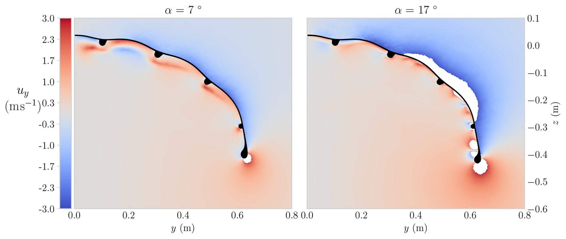
Figure C1 Spanwise slices of the u_y flow fields from Viré et al. (2022) at α = 7° (left) and α = 17° (right), taken at $\mathrm{0.25}x/c$ from the leading edge. White regions indicate $\left|u_y\right|$ > 3 m s⁻¹.

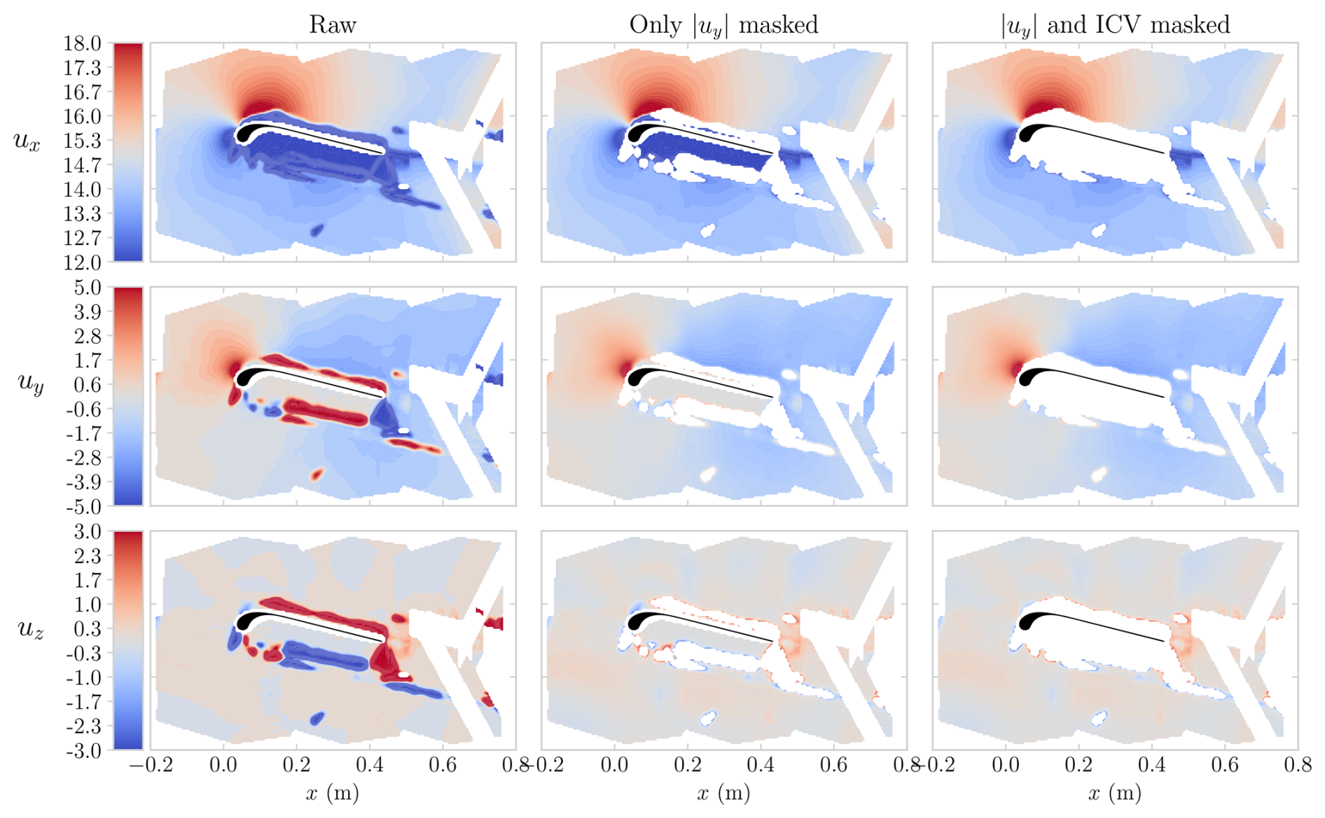
Figure C2 The process from raw to masked is illustrated, showing the velocity components u_x, u_y, and u_z at plane Y1, α = 7°.

An ICV (inverse coefficient of variation)-based filter was applied to suppress residual temporally incoherent vectors. The ICV is defined as

$$\begin{array}{}\text{(C1)}& \text{ICV}\left(i\right)=\text{median}\left({\displaystyle \frac{\left|\stackrel{\mathrm{‾}}{u_x}\right(i\left)\right|}{{\mathit{\sigma }}_{u_x}\left(i\right)}},{\displaystyle \frac{\left|\stackrel{\mathrm{‾}}{u_z}\right(i\left)\right|}{{\mathit{\sigma }}_{u_z}\left(i\right)}}\right),\end{array}$$

where $\stackrel{\mathrm{‾}}{(\cdot )}$ and σ_(⋅) denote the ensemble mean and standard deviation; only components with ${\mathit{\sigma }}_{(\cdot )}>{\mathit{\sigma }}_{min}$ = 10⁻⁶ m s⁻¹ are included to avoid division by near-zero variance, and u_y is excluded. The per-component ratios are combined using a median reduction. Vectors with ICV < 2.0 are rejected at both angles of attack. Reflection-induced correlation failure collapses the mean and inflates the standard deviation, yielding low ICV, whereas well-resolved regions retain high values. At α = 17°, genuine flow separation produces a similar low-ICV signature; the filter is therefore spatially restricted to the region below a linear line fitted through the rear 50 % of the airfoil surface, confining rejection to the near-surface reflection-prone zone and avoiding masking of the separated flow region above the airfoil. The resulting rejection fractions f_ICV are reported in Table 4.

Appendix D: Stitching uncertainty

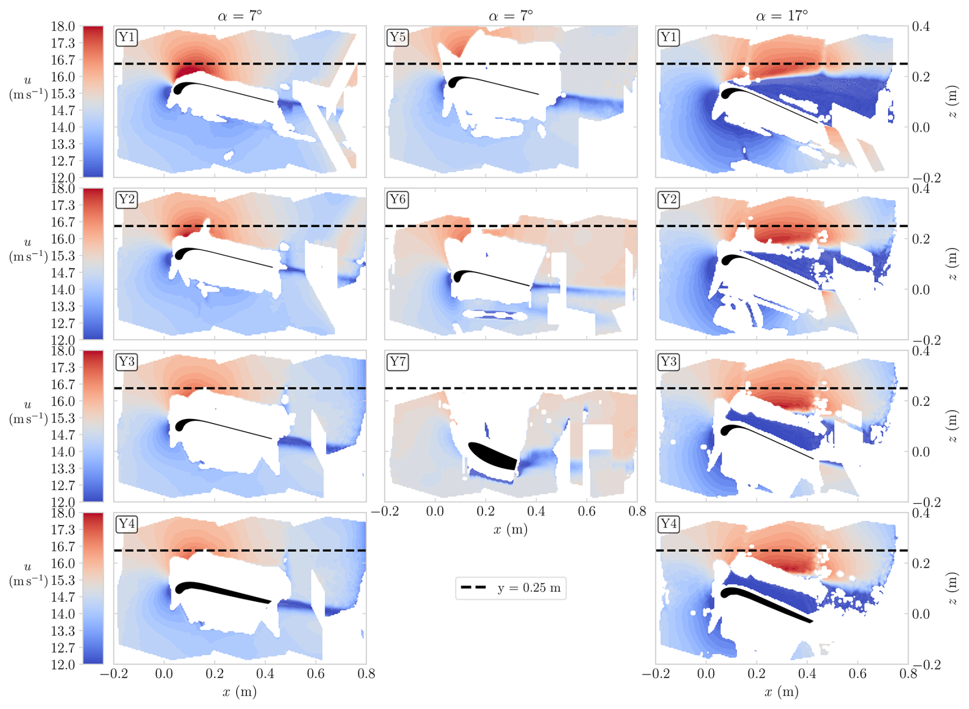
Figure D1 Stitched PIV velocity fields used to assess consistency across sub-plane overlaps. Fields are shown for multiple measurement planes Y_i at α≈ 7° (columns 1–2) and α≈ 17° (column 3). Colours indicate the velocity magnitude u, with the airfoil outline overlaid. The dashed black line at z = 0.25 m indicates the threshold above which overlap data are sampled for Table D1.

To quantify the consistency between adjacent PIV sub-planes after stitching, a stitching uncertainty was evaluated from the velocity differences in the overlap regions.However, missing vectors and locally degraded reconstruction quality in the overlap regions reduced the spatial coverage available for these comparisons and prevented robust averaging over the full overlap extents.Therefore, the reported stitching uncertainty was computed from a restricted subset of overlap points sampled above an upper-layer line at z = 0.25 m. This line was selected because, for the measurement planes emphasized in the paper and for those with comparatively lower uncertainty (Table 5), the reconstructed flow fields in this region remained qualitatively consistent. The measured velocity fields and the corresponding line used for the overlap analysis are shown in Fig. D1.

For each measurement plane Y_i, the streamwise overlap regions between adjacent sub-planes (X1–X2 and X2–X3) were analysed independently when present. Prior to comparison, the velocity fields from the two contributing sub-planes were subjected to identical validity filtering. Within each overlap region, the difference between the two sub-plane velocity fields was computed component-wise over all grid points where both fields remained valid.

For each overlap pair k, the root mean square (rms) of the difference field for a given velocity component was calculated as

$$\begin{array}{}\text{(D1)}& {\mathit{ϵ}}_{\text{stitch},k}=\sqrt{{\displaystyle \frac{\mathrm{1}}{N_k}}\sum _{j=\mathrm{1}}^{N_k}(u_{A,j}-u_{B,j}{)}^{\mathrm{2}}},\end{array}$$

where N_k denotes the number of valid grid points in overlap region k, and u_A,j and u_B,j are the velocity components from the two sub-planes at grid point j.

The reported stitching uncertainty is defined as the arithmetic mean of the per-overlap rms values,

$$\begin{array}{}\text{(D2)}& {\stackrel{\mathrm{‾}}{\mathit{ϵ}}}_{\text{stitch}}={\displaystyle \frac{\mathrm{1}}{K}}\sum _{k=\mathrm{1}}^K{\mathit{ϵ}}_{\text{stitch},k},\end{array}$$

where K=2 corresponds to the two adjacent overlap pairs (X1–X2 and X2–X3).

This metric does not represent a full measurement uncertainty. Instead, it provides a local measure of consistency between independently acquired sub-planes at identical spatial locations and, therefore, serves as an indicator of the magnitude of residual differences across stitched regions. The resulting rms differences for all available measurement planes and angles of attack are summarized in Table D1.

Overall, the overlap-based rms differences in Table D1 are typically of order 𝒪(10⁻¹)–𝒪(1) m s⁻¹. For comparison, type A showed smaller uncertainties of 0.07–0.10 m s⁻¹ at α = 7° and 0.18–0.26 m s⁻¹ at α = 17°, indicating that stitching-related deviations are approximately 3–10 times larger and thus represent a non-negligible systematic contribution in the overlap regions. Taking ∼ 1 m s⁻¹ as a pragmatic upper bound for acceptable stitching deviations, most planes at α = 7° fall within this range, with larger values being confined to regions of degraded reconstruction quality. At α = 17°, rms differences exceed this threshold in several planes, consistently with increased unsteadiness, masking, and reduced correlation quality under stalled conditions.

Table D1 Stitching uncertainty quantified as the root-mean-square (rms) difference in the overlap regions, reported for the stitched velocity components u, v, and w. Values are aggregated per measurement plane.

NA: not available.

Appendix E: Defining boundary curves

To obtain aerodynamic properties of a flow field, the methods described in Sect. 2.7 are used and require a boundary curve. Two curve shapes were used, an ellipse and a rectangle, illustrated for both CFD and PIV at Y2 and Y5 with α = 7° in Fig. E1. The boundary curves are described by a number of nodes N_b. For each boundary node N_b,i, the flow field data inside a square of 0.05 m ×  0.05 m centred at N_b,i was interpolated to populate N_b,i.

When analysing the PIV measurement planes, certain boundary curves cross regions without flow field data. Each encountered empty flow field node inside an interpolation square is populated by an additional interpolation using the neighbouring nodes. Examples of interpolation squares crossing initially empty flow fields are indicated by the black squares in the second column of Fig. E1.

The boundary curves are defined by an x centre coordinate x_b, a z centre coordinate z_b, rotation angle, width W_b, height H_b, and N_b. The centre locations are set to be equal to the airfoil centroids. To determine suitable W_b and H_b values, a convergence study was done on the lift calculated with Noca's method C_l,Noca and the circulation Γ.

The sensitivity results are shown for Y2 with α = 7° in Fig E2. The first column shows the variation when only changing N_b, where both CFD and PIV results show a converging trend for C_l,Noca and Γ. For PIV, the rectangle shape predicts different values. In the second and third columns, the boundary width W_b and height H_b are shown. Each marker is coloured by the percentage of grid points inside the interpolation squares whose u value was missing and therefore locally interpolated, normalized by the total number of grid points inside these squares. Cases exceeding 20 % are excluded from the dataset. The CFD results exhibit good convergence for variations in both W_b and H_b. Both the ellipse and rectangle shapes show close agreement in terms of the values of C_l,Noca, with only a small deviation in the circulation, Γ. In contrast, the PIV results often fail to converge, with frequent misalignment between the ellipse and rectangle shape predictions.

The “optimal” number of nodes was determined considering the convergence of circulation Γ and the drag predicted by Noca's method C_d,Noca. All planes converged when increasing N_b. A value of 360 nodes was selected for all planes. Determining the parameters W_b and H_b was done iteratively for each plane and α separately. The resulting curves were checked visually and numerically using the percentage of interpolated empty flow field points to ensure that the curve crossed as many as possible through the measured flow field. On top of that, the neighbouring points, e.g. not only 0.4 m wide but also 0.41 m wide, were checked using the same criteria. A vertical line is present in all plots, indicating the selected values, which, together with the centres, are reported in Table F1 in Appendix F for all planes.

As the sensitivity analysis showed that the PIV flow field is sensitive to the boundary curve parameters, the analysis was conducted on 36 combinations of W_b and H_b and then was averaged to reduce inconsistencies. The 36 combinations comprise six W_b values and six H_b values and span a ±5 % region around the “optimal” value, indicated in the plots by the vertical grey band. A sensitivity analysis was performed on the rotation angle over a sweep of ±10°; differences in C_l,Noca and Γ of less than 0.01 were observed and are not reported here.

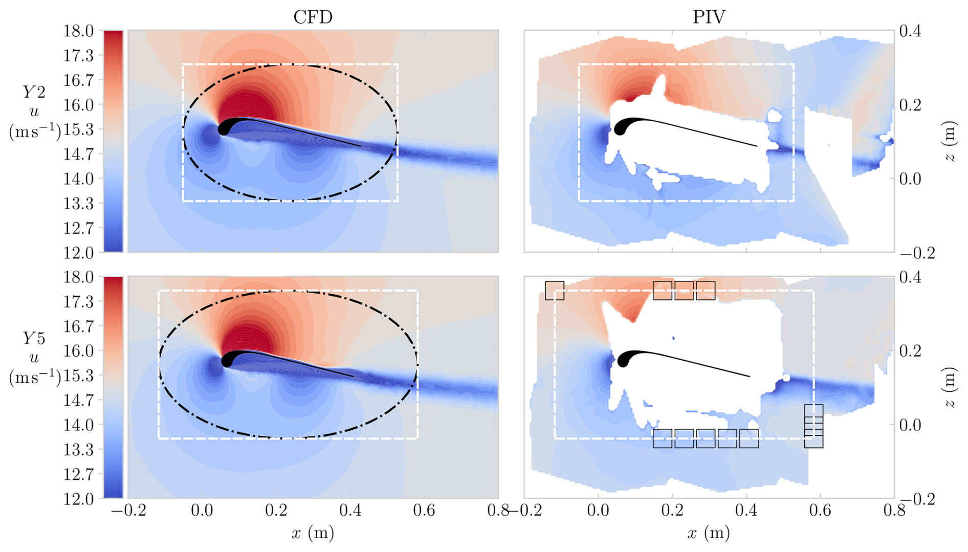
Figure E1 The left column shows CFD, and the right column shows PIV, both coloured by the velocity magnitude u. The top row contains the Y2 plane, and the bottom row contains the Y5 plane, both measured at α = 7°. The white rectangle and the black ellipse represent the two investigated boundary shapes, and the smaller black squares in the right column represent the PIV locations for which additional interpolation was required to ensure sufficient data presence for populating the boundary nodes.

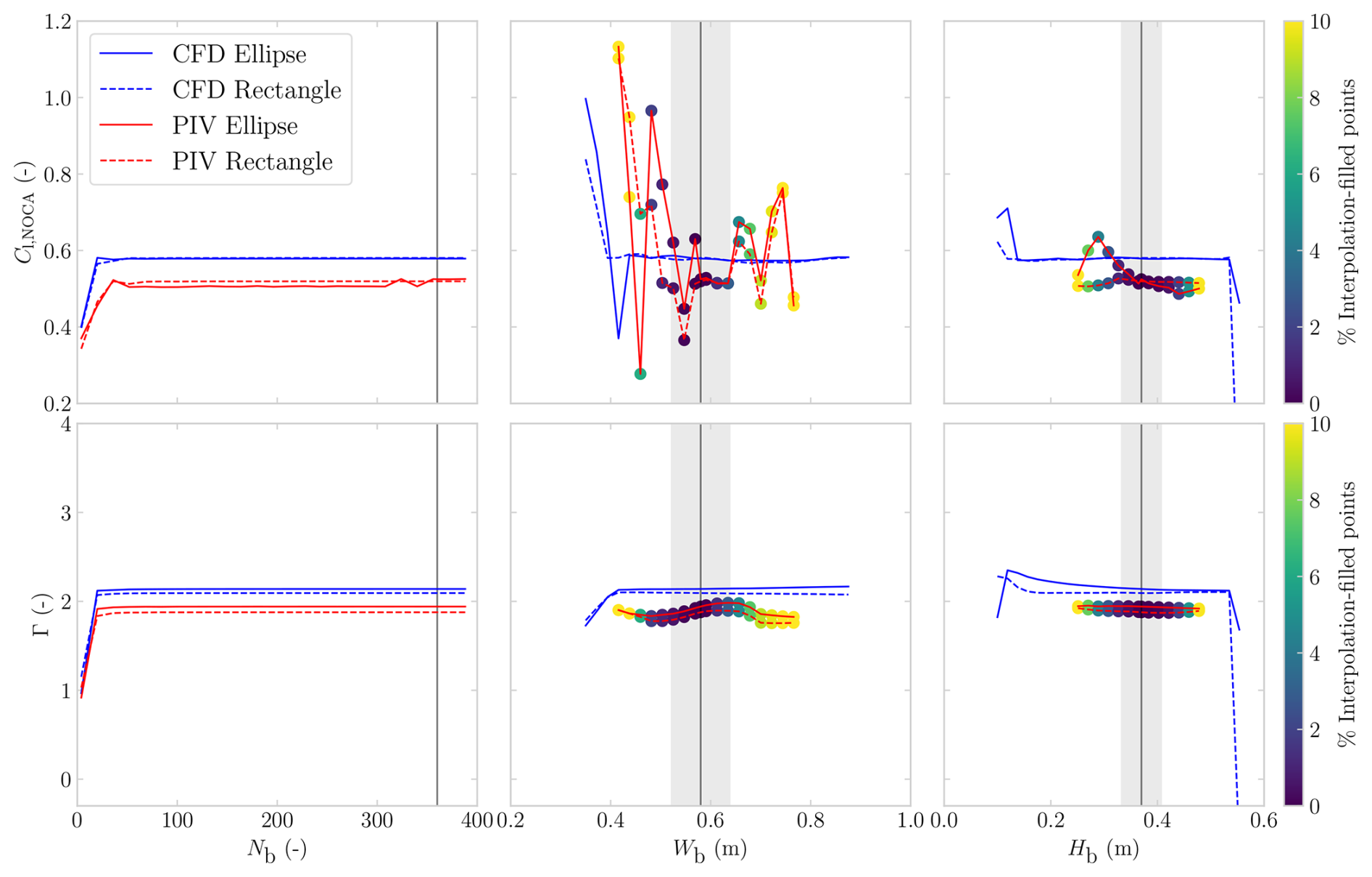
Figure E2 Convergence analysis for Y2 boundary curve setting, i.e. N_b, W_b, and H_b, used for the calculation C_l,Noca presented in the top row and Γ reported in the bottom row. Each plot contains a vertical line, indicating the determined “optimal” value, and the vertical grey band indicates the region that was used for averaging.

Appendix F: Tabulated quantitative results

Table F1 Aerodynamic coefficients for the measured PIV and simulated CFD of different planes using NOCA, Kutta, and pressure integration reference values.

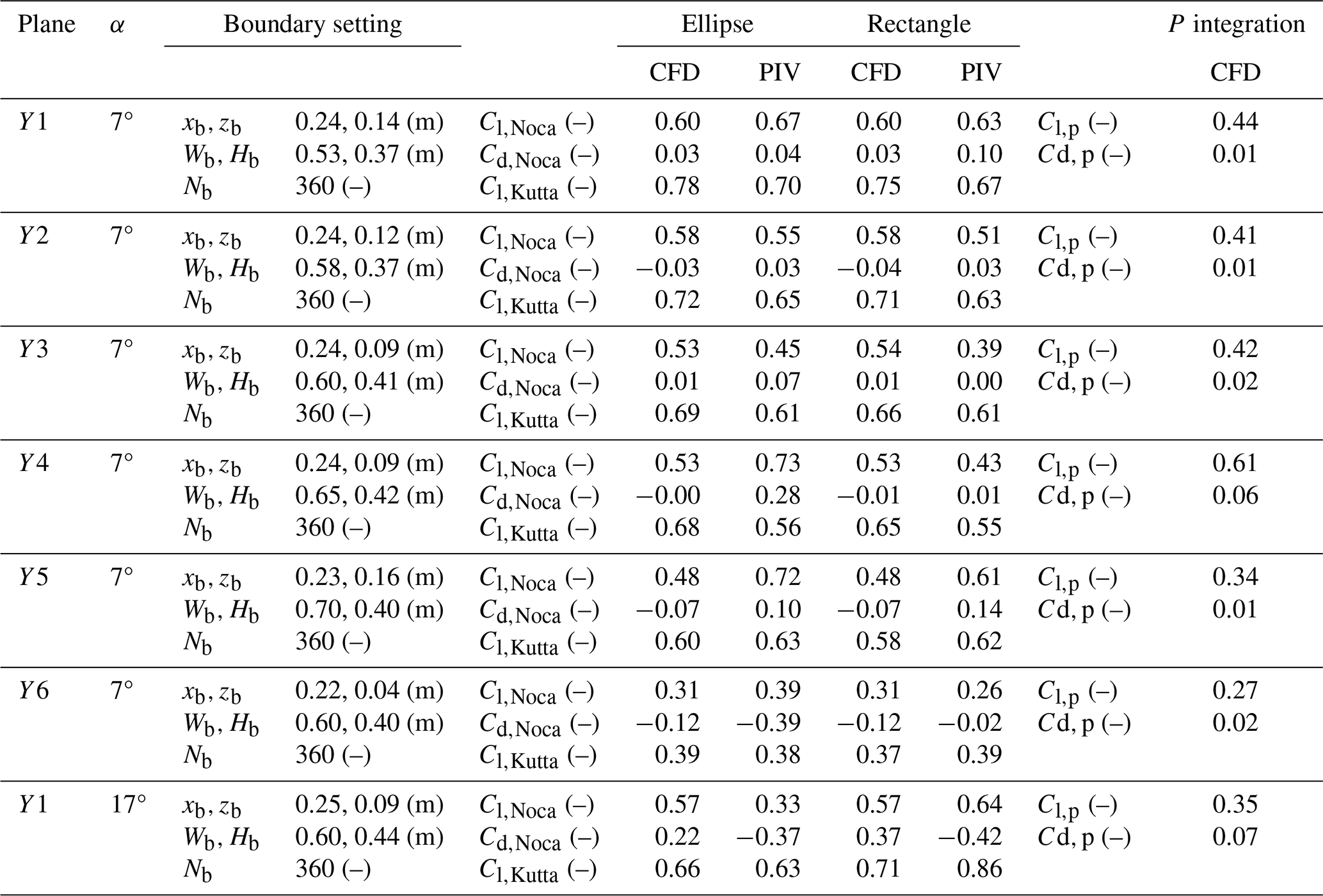
The quantitative results, underlying Fig. 9, are shown in Table F1 for future use. Only planes containing sufficient data for boundary curve interpolation are included in the analysis. Since the table differentiates between elliptical and rectangular contours, it further highlights that the CFD results are comparatively insensitive to contour shape compared with the PIV results. Table F2 shows that the quadratic correction term associated with the perturbation velocity is consistently negative across all evaluated cases, thereby explaining the systematic overprediction of lift by the Kutta–Joukowski estimate.

Table F2 Diagnostic comparison between the inviscid, non-rotational Noca contribution and Kutta–Joukowski lift, $\mathrm{\Delta }{C}_{\text{l}}=C_{\mathrm{l},\text{inv},\text{nonrot}}-C_{\mathrm{l},\text{Kutta}}$. Values correspond to the average over ellipse and rectangle contours.