Aeroelastic instabilities of the IEA 15 MW rotor during extreme yaw maneuvers

This study explores the aeroelastic behavior of the IEA 15 MW wind turbine rotor during dynamic yaw maneuvers under storm conditions through high-fidelity computational fluid dynamics (CFD) simulations. The focus is on blade vibration responses to a variety of yaw misalignments while maintaining constant pitch and azimuth settings. Utilizing the geometrically exact beam theory (GEBT) and the OpenFOAM framework, the study reveals that certain yaw angles lead to significant edgewise blade vibrations, with distinct responses being observed among the rotor's three blades. Detailed analysis of one blade at varying fixed yaw angles, employing Hilbert–Huang transformation, uncovers a lock-in effect where flow structures synchronize with the blade's eigenfrequencies, resulting in pronounced blade tip vibrations. Key findings indicate that the most substantial vibrations occur during specific yaw angles, suggesting that the rotor's structural integrity could be compromised under certain dynamic conditions. This work enhances the understanding of aeroelastic instabilities during off-design yaw maneuvers and highlights the need for operational strategies in managing rotor performance during extreme conditions.

1 Introduction

The global transition towards sustainable energy sources has become increasingly urgent due to the pressing challenges posed by climate change, energy security, and the depletion of fossil fuels. Renewable energy, particularly wind energy, plays a central role in this transition, offering a clean and accessible alternative to traditional energy resources (IEA, 2023). As technology advances, the deployment of wind turbines continues to expand. In this context, the economic demand for low prices in a highly competitive market leads to larger rotor diameters as larger rotors capture more energy from the wind flowing past the rotor disk, while the cost impact on other turbine components, such as the nacelle, tower, or foundation, remains limited (Bolinger et al., 2021). Consequently, slender, lightweight structures emerge as a direct result of rotor diameter growth, provided that the impact on other turbine components remains limited, with higher blade flexibility accompanying this growth. This ultimately leads to reduced levelized costs of energy (Veers et al., 2019). In this regard, softer and more aerodynamically efficient designs move closer to stability boundaries that could lead to structural failure (Veers et al., 2023), necessitating a deeper understanding of the complex dynamics involved in wind turbine operation. In particular, investigating vibration phenomena like stall- (SIVs) and vortex-induced vibrations (VIVs) is essential for optimizing performance and ensuring the structural integrity of these systems. Severe VIV normally occurs when shed vortices build a coherent structure in the wake of the blade (Dowell, 2022; Skrzypiński et al., 2013). In wind energy, this typically requires locked rotor conditions or idling and an inability to realign with the wind. Such conditions may arise during storms, grid loss, or maintenance. SIV occurs when larger parts of the blade operate in stall, and a negative lift-to-angle-of-attack gradient leads to negative aerodynamic damping. Consequently, the lift force is in phase with the blade motion, supporting the growths of blade vibrations (Dowell, 2022; Hansen, 2007).

Stall- and vortex-induced vibrations are critical phenomena that can significantly impact the performance and structural integrity of various engineering systems, particularly in the fields of renewable energy (Veers et al., 2023) and aerospace engineering. The investigation of these vibrations is essential to understand the underlying mechanisms, predict their occurrence, and develop effective mitigation strategies. Previous studies highlight the relationships between flow dynamics, structural responses, and environmental conditions, emphasizing the need for advanced modeling and experimental approaches (Hansen, 2007; Zou et al., 2015). By addressing these challenges, researchers can enhance the reliability and efficiency of systems such as wind turbines and marine structures, ultimately contributing to safer and more sustainable engineering practices. In this regard, Grinderslev et al. (2023) carried out a numerical study on turbulence modeling and grid characteristics in computational fluid dynamics (CFD) analyses of a 10 MW turbine. The study found that the numerical results are more sensitive to low-inclination flow, i.e., reduced spanwise flow. This sensitivity is connected to the influence of wake vortex structures on the power injected into the structural system by aerodynamic loads. This impact of correlated vortex structures on the blade vibrations is also discussed in Heinz et al. (2016) on a wind turbine blade of similar size in standstill. With such vortex structures being shed at frequencies in the vicinity of the first edgewise eigenfrequency, a substantial edgewise vibration growth is found to be present. In Horcas et al. (2020), the impact of the blade geometry on near-wake vortex structures is being discussed. Here, in particular, the shape of the blade tip is analyzed for contributions to changes in the wake using CFD simulations of rigid and flexible blade conditions in standstill. It has been found that bending the blade tip out of the rotor plane leads to an earlier breakdown of the vortex tubes shed from the tip. Additionally, depending on the tip geometry, wake lock-in can be shifted towards higher inclination angles or mitigated completely. A closer look into the impact of different fixed wind inflow angles was performed in Horcas et al. (2022) using fluid–structure interaction (FSI) on a 10 MW rotor blade. In a variety of CFD simulations the authors analyzed the impact of spanwise flow from the blade tip towards the blade root. It is shown that blade vibrations are found to be present in regimes of high- and low-inclination angles. The studies described above conduct analyses on isolated blade setups. However, Pirrung et al. (2024) demonstrated that, in a structurally fully coupled turbine, tower torsion drives substantially larger blade deflections, which markedly affect power injection near the blade tip. By contrast, such vibration amplitudes are not reached in isolated blade setups, and the resulting power injection differs from that of the fully coupled system.

Existing studies on inclined inflow and wake-vortex-induced vibrations have so far mainly considered turbines up to a 10 MW scale and typically focused on fixed or discretely stepped yaw angles rather than yaw-based load mitigation strategies. This leaves a gap in understanding for larger, more representative turbines in the 15 MW class and for storm fault scenarios in which a dynamic yaw sweep, as assumed in this study, is used to reduce extreme loads. To address this gap, this paper presents a comprehensive high-fidelity CFD analysis of the IEA 15 MW turbine under an extreme storm fault scenario, in which one blade fails to pitch to feather and remains at a fixed pitch angle of −60°, while a dynamic yaw maneuver drives the rotor towards a misalignment of −90° so that the inflow approaches the rotor from the side and the mean aerodynamic loads are minimized. The present work focuses on the unintended side effects of this control strategy, namely the aeroelastic blade vibrations that may arise during the yaw sweep.

This investigation is extended using isolated blades subjected to side inflow, progressing systematically from simulations with rigid blades to fully fluid–structure-coupled analyses. This staged approach enables us to identify the onset of aeroelastic vibrations and to characterize the lock-in between unsteady wake structures and the first edgewise structural frequency. A key contribution of this paper is the detailed examination of blade response using the Hilbert–Huang transformation (Huang et al., 1998) applied to various aerodynamic signals. This method links time-varying frequencies in the aerodynamic loads to blade vibration responses that are not revealed by a standard fast Fourier transform (FFT). The findings highlight that, even under a yaw control strategy specifically designed to alleviate loads in storm conditions, certain dynamic flow–structure interactions can trigger significant blade vibrations that should be explicitly considered in the design process and in future design standards.

2 Numerical methods and setup

To investigate blade oscillations of a large wind turbine in relation to yaw misalignment during storm conditions, simulations of the IEA 15 MW reference wind turbine (Gaertner et al., 2020) are conducted. With a rotor diameter of 240 m, this wind turbine is classified as being above average in size compared to currently installed machines (GWEC, 2025). Furthermore, several numerical studies using various codes for this specific wind turbine have been carried out within IEA Wind TCP Task 47 “TURBINIA”, providing a basis for comparison (Schepers et al., 2025). This is particularly significant, as no measurement campaigns have been conducted for the generic model against which simulations could be validated.

2.1 Numerical discretization schemes and solver setup

All simulations in this study were conducted using the open-source software OpenFOAM (2023). The incompressible, transient flow solver pimpleDyMFoam is integrated with the in-house non-linear structural finite-element beam solver BeamFOAM (Dose, 2018). The structural beam implementation utilizes the finite-element GEBT formulation originally proposed by Reissner (1972) and Simo (1985), enabling the resolution of large deformations in wind turbine blades. Temporal integration of these beams is performed using the second-order generalized-α scheme (Arnold and Brüls, 2007). The coupling of fluid and structural dynamics is implemented within the OpenFOAM framework without requiring external code communication and operates in a loose-coupling manner, where information is exchanged once per time step.

The incompressible, transient flow is simulated using the hybrid Spalart–Allmaras delayed detached eddy simulation method (Spalart et al., 2006). A second-order implicit backward method is employed for time advancement. Spatial discretization utilizes a second-order accurate Gauss linear scheme for gradient terms and a first-order Gauss upwind scheme for divergence terms. The rotor rotation is modeled using sliding-mesh interfaces between the three blade grids, the rotor disk, and the far-field grid (Dose et al., 2018; Höning et al., 2024; OpenFOAM, 2023).

2.2 General case setup

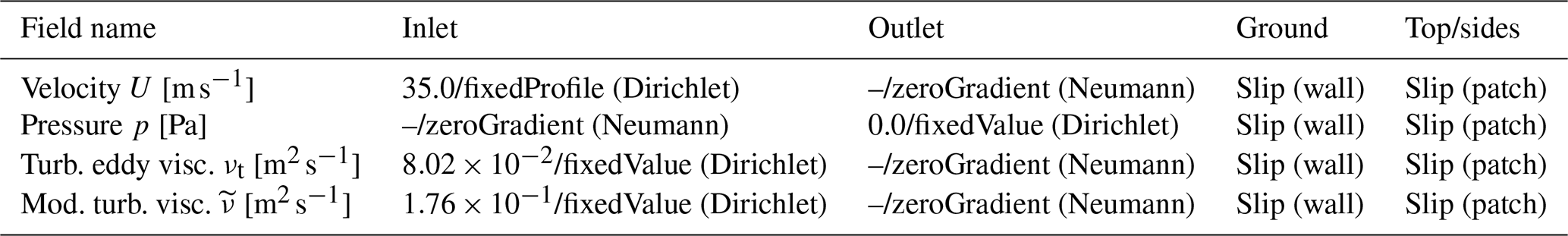
Velocity, pressure, and turbulence boundary conditions are set as shown in Table 1. Here, a fixed profile boundary condition for velocity follows the atmospheric power law function as follows:

$$\begin{array}{}\text{(1)}& u_x\left(z\right)=u_{x,\mathrm{hub}}\cdot {\left({\displaystyle \frac{z}{z_{\mathrm{hub}}}}\right)}^{\mathit{\alpha }},\end{array}$$

where u_x describes the velocity in the x direction as a function of the height z. and u_x,hub is the fixed hub height wind speed of 35 m s⁻¹. z_hub is defined as the hub height of 150 m, and α represents the shear factor exponent chosen as 0.11 to form a realistic inflow. Velocity components in the y and z direction are set to 0 m s⁻¹. Turbulent viscosity values were chosen to reflect a turbulence intensity of 0.1 % in the rotor plane. The choice was made to minimize the impact of the incoming flow on the breakdown of vortices shed from the blades.

Table 1 Boundary conditions and values of all simulated cases according to OpenFOAM nomenclature.

The case setup overview is shown in Table 2, where an azimuth angle of 0° corresponds to a blade pointing upwards, and a positive rotation is defined in a clockwise direction. The pitch angle is defined about the pitch axis, with a negative sign corresponding to a pitch to feather. The yaw angle is defined to be positive around the vertical axis (0 0 1).

Table 2 Overview of the main rotor characteristics of the IEA 15 MW reference turbine and the investigated conditions.

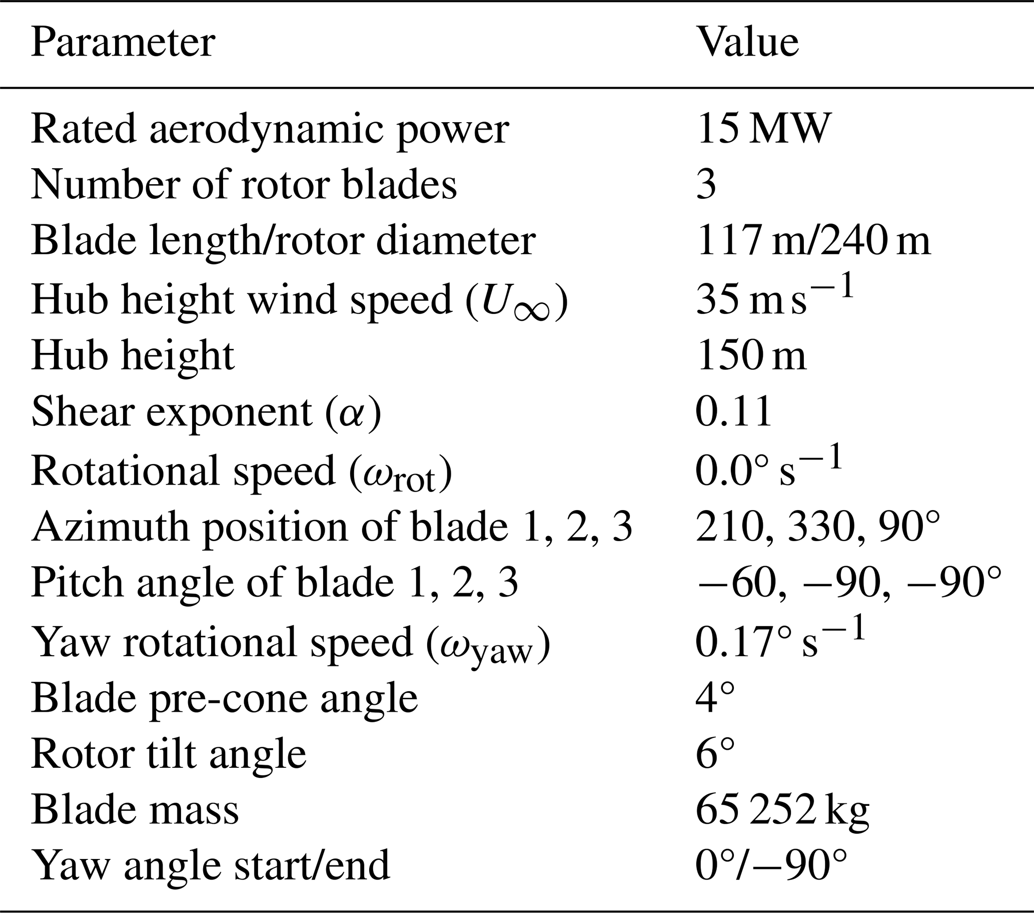
In Sect. 3.1 the simulation of a three-bladed full rotor with blades pitched at different angles during a yaw maneuver with a locked rotor is examined. A tower is not included to be able to investigate the pure aerodynamic effects of the blades without further complexity introduced by blade–tower interaction. The constant pitch angles and fixed rotor azimuth are selected to both simulate the impact of a pitch motor failure, where blade 1 is stuck at −60°, and to induce a variety of inflow conditions across the range of simulated yaw angles. This setup was chosen in accordance with the International Electrotechnical Commission (IEC) standard 61400-1 Design Load Case 6.2, in which a connection to the electrical power network is lost (IEC, 2019). A control strategy is assumed, where the turbine yaws out of the wind using a power backup system to reduce rotor loads. Here one blade points into the wind, and the other two blades are equally inclined leeward. Additionally, in Sect. 3.2, an in-depth analysis of specific conditions for a single blade in stand-still is provided.

2.3 Numerical grid

All simulations performed in this study make use of the identical overall CFD domain dimensions. As visualized in Fig. 1, the inlet distance towards the center of the imaginary rotor plane measures 1200 m, which corresponds to five rotor diameters. The distance towards the sides and the top of the domain measures 3.5 D. The rotor center itself is located 0.625 D above the ground, which corresponds to the hub height of the IEA 15 MW turbine. A tower is not included in the setup. The hub height ensures that a reasonable shear profile can be injected into the simulation. The outlet of the domain is located 15 D downstream of the rotor plane to properly resolve the wake generated by the blades.

Figure 1 Rotor mesh dimensions making use of five sliding-mesh interfaces.

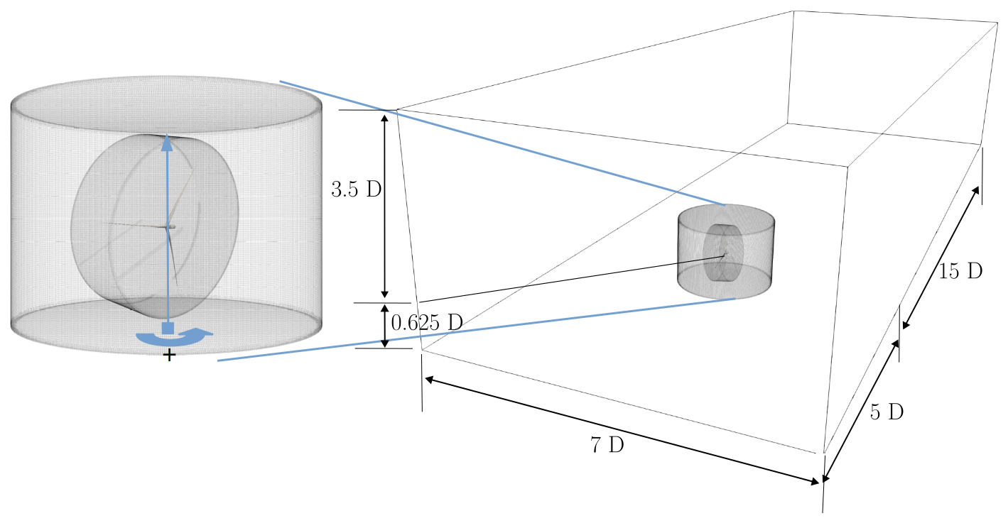
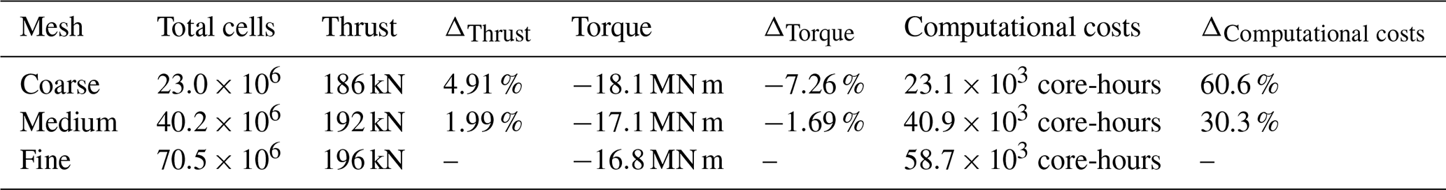
Blade meshes have been created using the in-house meshing tool BladeBlockMesher (Rahimi et al., 2016), which composes 2D sectional meshes into a 3D structured blade volume mesh, consisting only of hexahedral cells. For most first-layer cells, the y⁺ value is between 30 and 70, and a wall function ensures a consistent turbulent viscosity profile across all walls. When velocities near the blades are low and smaller y⁺ values are present, the wall function is automatically disabled to improve accuracy, for example, in regions of flow separation. Since no validation data are available, the choice of grid resolution is based on a grid dependence study. For that purpose, three differently refined meshes have been analyzed for blade 2 under inflow conditions of −37° yaw misalignment in standstill. The coarse mesh consists of 23.0×10⁶ cells, while the medium-refined grid consists of 40.2×10⁶ cells. The fine mesh has a total of 70.5×10⁶ elements. All three mesh directions have been refined simultaneously by ≈ 20 %, resulting in a global refinement factor of $F_{\mathrm{ref},\mathrm{1}}\approx \mathrm{1.75}$ from the coarse to the medium-refined grid and a refinement factor of $F_{\mathrm{ref},\mathrm{2}}\approx \mathrm{1.76}$ from the medium to the fine grid.

A forced-motion oscillation with a maximum of ≈ 6.8 m edgewise tip deflection amplitude in the shape and frequency of the first edgewise eigenmode is applied. This amplitude corresponds to approximately 5 % of the blade length and is considered to be a reasonable value for the analysis of edgewise vibrations of large turbine blades under storm conditions. For a 10 MW machine, Heinz et al. (2016) reported at least 2 % for an isolated blade, while Pirrung et al. (2024) reported 17 % using the full turbine. The amount of cells used for the three meshes and the corresponding thrust and torque deviations towards the results of the fine grid are listed in Table 3. All simulations covered a time span of 64.64 s and were averaged over the last 38 edgewise motion cycles (55.95 s). It is noted that the deviation of the thrust and torque results from the medium-refined mesh towards the fine mesh is less than 2 %. The deviations of the coarse mesh towards the fine mesh, on the other hand, show thrust and torque overshoots of 4.91 % and 7.26 %, respectively. Based on this, the medium-refined mesh configuration is used for the following simulations as it represents a reasonable compromise between computational costs (30.3 % cheaper than the fine case) and numerical accuracy. In this final setup, the blade mesh consists of 256 cells chordwise, and 60 cells are distributed in the blade-normal direction. The spanwise direction is resolved using 597 cells. To further validate the accuracy of this mesh, a configuration with the same cell resolution was previously employed in a code-to-code comparison for the IEA Wind TCP Task 47. This comparison, conducted under uniform steady-flow conditions for a turbine in operation, demonstrated good agreement with results obtained from other computational codes (Schepers et al., 2025).

Table 3 Differently refined grids used in the mesh dependence study. The relative thrust, torque, and computational cost deviation are defined with respect to the fine grid.

2.4 Structural model and discretization

Consistently with the generic HAWC2 design described in IEA Wind Task 37 (2020b), this study employs 26 iso-parametric beam elements per blade. Each element comprises two nodes with 6 degrees of freedom. Structurally, the rotor is modeled using three isolated beams, without taking into account the drive train, yaw bearing, or the tower flexibility to focus purely on the wind–blade interaction. In GEBT, the structural damping is applied as a viscous force F_d that is proportional to the strain rates:

$$\begin{array}{}\text{(2)}& {\mathit{F}}_{\mathrm{d}}={\mathit{\mu }}_s\mathbf{C}\dot{\mathit{e}},\end{array}$$

where μ_s reflects the damping coefficients, C denotes the cross-sectional stiffness matrix, and $\dot{\mathit{e}}$ represents the corresponding six strain components. Correctly setting the structural damping values is crucial for effectively modeling the interaction between fluid and structure as larger vibrations occur only when the aerodynamic forces surpass the structural damping. The damping coefficients μ_s have been adjusted to ensure that a blade, initially deflected at the tip and subsequently allowed to vibrate freely, exhibits logarithmic decrements of 2.98 % in the edgewise direction, 2.64 % in the flapwise direction, and 6.28 % in the torsional direction. The obtained values exhibit a marginal underestimation of the structural damping compared to the reference values of 3 %, 3 %, and 6 % (see Gaertner et al., 2020); however, they are deemed to be reasonable. Additionally, a slight underestimation can be regarded to be a conservative approach for the investigation of the vibration behavior of a wind turbine blade.

In Fig. 2, the first three structural modes are described. On the left side (Fig. 2a, c, and e), the mode shapes are shown, which are normalized by the maximum value of the dominant component. The lines labeled as “flap. ref.” and “edge. ref.” describe the reference shapes of the dominant modes in flapwise and edgewise directions, as described in IEA Wind Task 37 (2020a). It can be seen that the first flapwise and first edgewise mode shapes are also influenced by the respective other component. On the right-hand side, the corresponding phase shift between the dominant and the respective other component is described (see Fig. 2b, d, and f). A 180° offset for the first flapwise mode means that the maximum tip deflection towards the pressure side is in phase with the minimum edgewise tip deflection with respect to the trailing edge. The mode shapes demonstrated a strong agreement with the analytical reference.

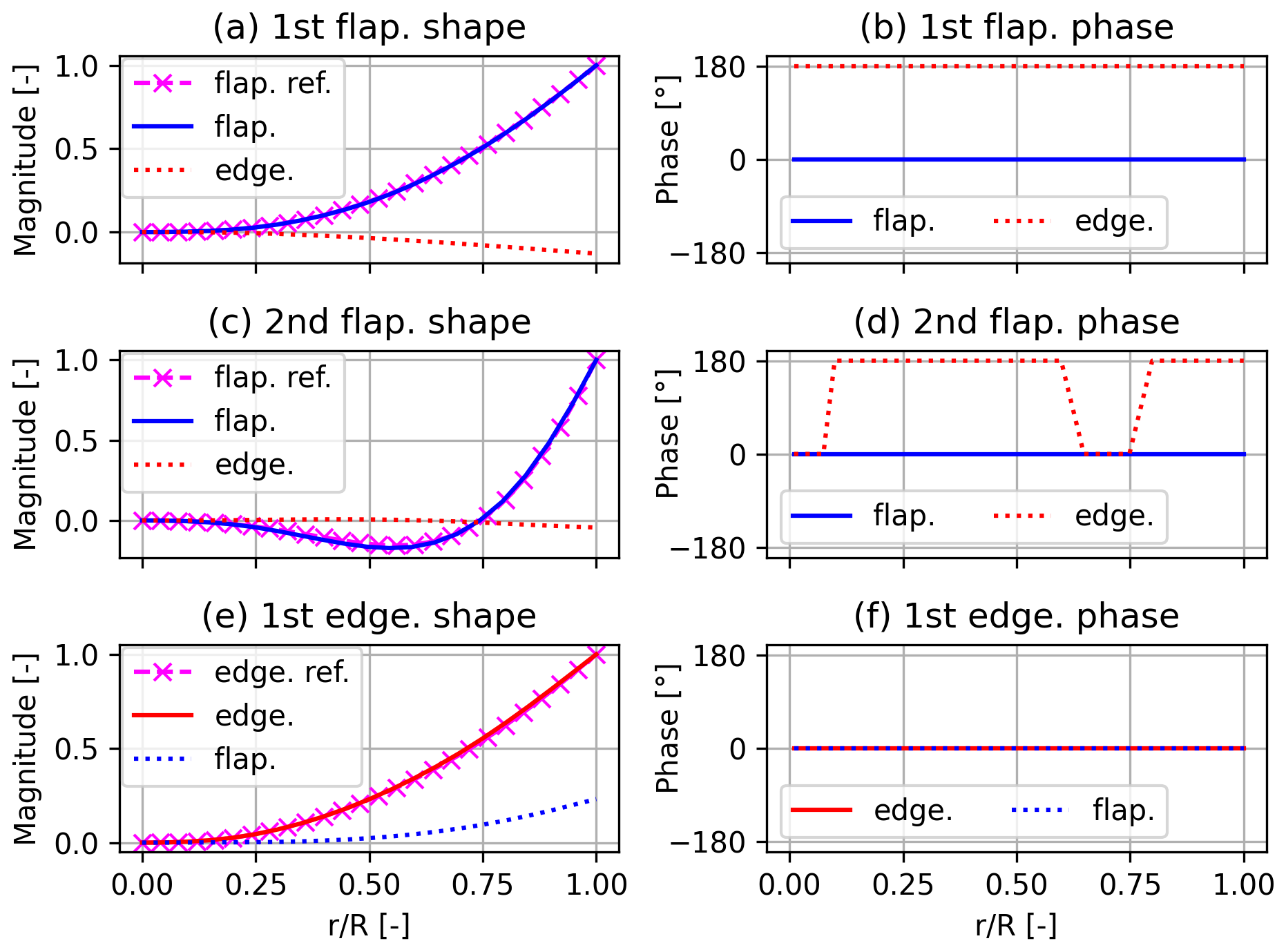
Figure 2 First three modes of the IEA 15 MW blade in shape (a, c, e) and phase (b, d, f). Edgewise components are labeled as “edge.”, and flapwise components are labeled as “flap.”. Reference values are taken from IEA Wind Task 37 (2020a) and are supplemented with the designation “ref.”.

2.5 The Hilbert–Huang transformation

The analysis of force and flow frequencies in Sect. 3.2.5 makes use of the Hilbert–Huang transformation (HHT). The reasoning behind choosing this method was the difficulty of drawing proper conclusions regarding the time–frequency behavior using standard fast Fourier transformations. HHT provides insights into how the energy of a signal is distributed between its inherent frequencies (Huang et al., 1998). For that purpose, it is necessary to decompose the multi-component signal into separate signals, each of which falls within a narrow frequency range. This is achieved via a technique known as empirical mode decomposition (EMD). Once the component frequencies are obtained, the Hilbert transform is applied separately to each component to extract the instantaneous frequencies.

As described by Huang et al. (1998), the EMD is used to extract signal components that have distinct timescales from a given complex signal. Here, the timescales are determined by the intervals between the local minima or maxima of the given signal that are being used for the construction of cubic splines that form an envelope for the upper and lower bound of the signal and that are being used to generate a signal's intrinsic mode functions (IMFs). In a repetitive sifting procedure, a signal X(t) can be decomposed in its inherent IMFs. Following the description of Huang et al. (1998), the local maxima and minima are connected using cubic splines to produce the upper and lower envelope, respectively. Their mean is referred to as m₁ so that the first component is defined as the difference between the mean and the original signal:

$$\begin{array}{}\text{(3)}& X\left(t\right)-m_{\mathrm{1}}=h_{\mathrm{1}}.\end{array}$$

In the case where h₁ fulfills the requirements described by Huang et al. (1998) that no local maxima are found for values below 0, it already forms the first IMF. Otherwise, the sifting process is repeated k times, where its respective preceding sifting result h_1(k−1) is considered to be the input signal, until the requirements are fulfilled. It then forms the IMF as follows:

$$\begin{array}{}\text{(4)}& h_{\mathrm{1}(k-\mathrm{1})}-m_{\mathrm{1}k}=h_{\mathrm{1}k}={\mathrm{IMF}}_{\mathrm{1}}.\end{array}$$

IMF₁ should contain the finest scale of the input data. If it is separated from the original data, a new signal r₁ is created as

$$\begin{array}{}\text{(5)}& X\left(t\right)-{\mathrm{IMF}}_{\mathrm{1}}=r_{\mathrm{1}}.\end{array}$$

Here, r₁ still contains the information of the larger scales and can be treated similarly to the original data to iteratively generate the IMFs of the longer period components. Finally the procedure is stopped when the residual becomes monotonic or small, such that the summation of all IMFs gives the original signal as follows:

$$\begin{array}{}\text{(6)}& \sum _{i=\mathrm{1}}^n{\mathrm{IMF}}_i+r_n=X\left(t\right).\end{array}$$

Applying the Hilbert transform on each IMF component gives insights into the original signal's frequencies and its respective power. For the investigations within this work, the Python package described by Quinn et al. (2021) is used.

3 Results and discussion

The following sections describe the results of the investigated scenarios. In Sect. 3.1, the full rotor simulation during a yaw control maneuver from 0 to −90° is described. A critical yaw misalignment region is identified in which blade vibrations occur on one blade. In Sect. 3.2, the critical blade is isolated under stand-still conditions to provide an in-depth analysis of the driving mechanisms of this instability and to examine the underlying aerodynamic characteristics. For that purpose, a frequency analysis is conducted at one representative radial station on the blade and in the near-wake.

3.1 Yaw maneuver of the full rotor

In Fig. 3 the blade tip edgewise vibrations are shown for all three blades during the dynamic yaw maneuver from 0 to −90°. The storm conditions are simulated with a fixed azimuth angle so that each blade is facing different inflows. The yaw rotational speed ω_yaw was set to 0.17° s⁻¹, chosen as a realistic yaw rate estimate for this turbine size. Due to the huge amount of computational effort of 7987 core-hours per degree, the maneuver is split into three parts, each covering one-third of the maneuver. Due to the initial impact of the gravity force, the blades show a minor deflection at the beginning of each maneuver phase. It can be seen that blade 2 in particular shows a relevant response towards the incoming flow, with vibrations of more than 3 m amplitude. The response of blade 2 is therefore analyzed in more detail.

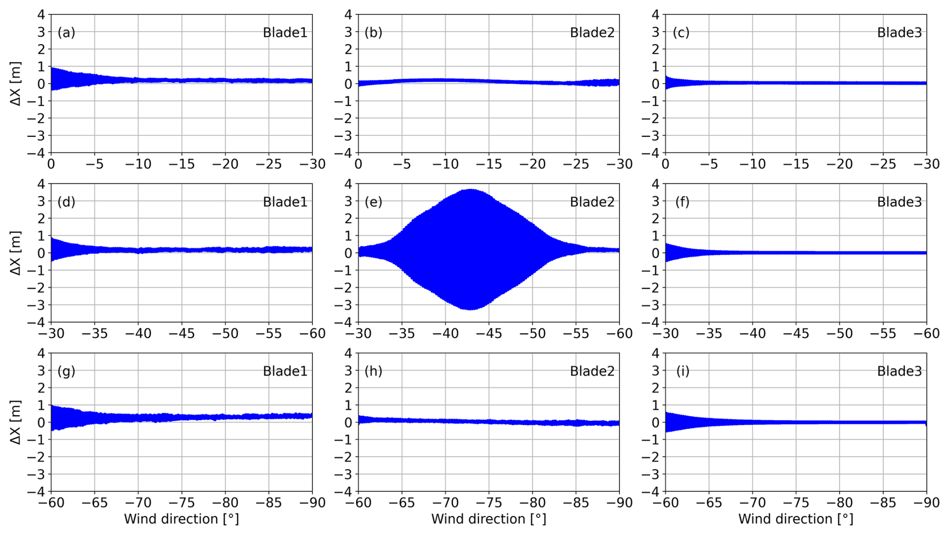
Figure 3 Edgewise blade tip displacement of all three blades during a yaw maneuver. Panels (a) to (i) show the tip displacement for all three blades separately and for wind direction intervals of 30°.

3.1.1 Blade response during vibration ramp up

A closer look at the tip oscillations of blade 2 (see Fig. 3e) reveals a vibration ramp up between −30 and −43° yaw misalignment. This ramp up can be visually split into two segments: from −30 to −33°, where amplitudes show a minor increase, and from −33 to −43°, where the growth rate of the tip displacement is larger, reaching a maximum tip displacement amplitude of 3.5 m at the end of the segment.

When looking into the total energy exchange between fluid and solid for this period, the edgewise excitation becomes more evident. In this context, the aerodynamic energy E_node is utilized, which is calculated via the force projection of each blade surface face onto the beam nodes as follows:

$$\begin{array}{}\text{(7)}& E_{\mathrm{node}}=\underset{t_{\mathrm{0}}}{\overset{n\cdot T}{\int }}{\mathit{F}}_{\mathrm{aero}}\cdot \mathit{u}\mathrm{d}t.\end{array}$$

Here, t₀ denotes the time at which the first vibration cycle begins, while T signifies the duration of each deformation period. The number of cycles is represented by n, and u denotes the velocity of the node. The instantaneous aerodynamic force F_aero acting on each beam node is computed using a weighted projection method, which employs the internal shape function of each beam element to project the forces from the surface faces onto the nodes of the element.

In Fig. 4 the summed edgewise (panel a) and flapwise (panel b) energy for each monitored spanwise position is shown. A positive energy value corresponds to energy being injected into the blade structure, and a negative energy value corresponds to energy being absorbed by the fluid (i.e., aerodynamic damping). For the edgewise component in Fig. 4a, a relatively weak damping for the inner half of the blade is visible, where the minimal negative value corresponds to −19 kJ. The majority of the exchanged edgewise energy is found for the outer half of the blade, with a maximum value for a relative spanwise position of 0.9 at a magnitude of 80 kJ. The total net energy for the ramp-up phase results in 240.86 kJ, which means that energy from the fluid is transferred into the blade and leads towards increasing edgewise deformations. A contrary picture is shown for the flapwise component in Fig. 4b. The majority of the blade is found to be exposed to negative energy exchange, which means that the flapwise vibration direction of the blade is being damped out. The total sum of flapwise energy is found to be −200.14 kJ.

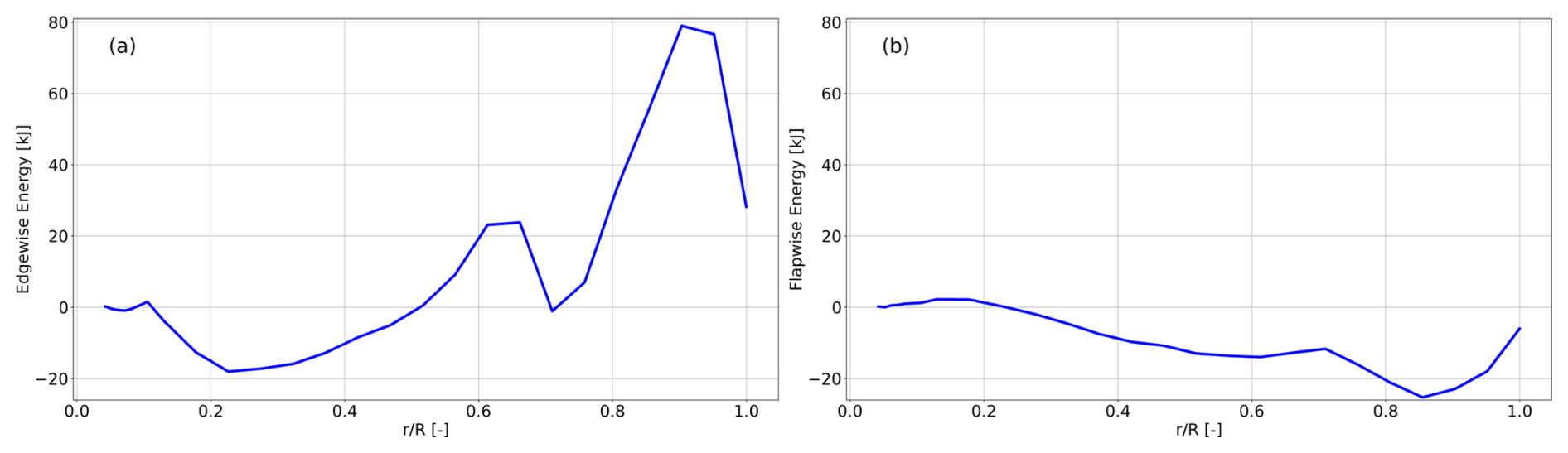
Figure 4 Energy per node of blade 2 along the blade span accumulated for the dynamic change of the yaw misalignment between −33 and −43° for (a) the edgewise direction and (b) the flapwise direction.

3.1.2 Blade response during vibration damping

For yaw misalignments between −43 and −53°, the edgewise vibration amplitudes of blade 2 decrease linearly until almost the whole vibration is damped out. This can also be seen in Fig. 3e. The paths of the displacement peaks almost mirror the blade behavior of the ramp-up phase.

A closer look at the edgewise energy over relative span shows two large damping regions on the blade (see Fig. 5a). From $\mathrm{0.05}\le r/R\le \mathrm{0.45}$ the summed edgewise energy is negative, i.e., contributes to the damping of the motion in this direction. The highest damping energy magnitude is found around $\mathrm{0.19}r/R$, with a value of −17 kJ. At $\mathrm{0.61}r/R$ the summed section energy contributes to excitation, with a peak value of ≈ 42 kJ. From $\mathrm{0.65}\le r/R\le \mathrm{1.0}$, the blade sectional energy contributes to the blade vibration damping, with its highest damping magnitude being −27 kJ at $r/R=\mathrm{0.7}$. Although the mid part of the blade is extracting energy from the fluid, the total edgewise energy exchange summed over the whole blade span within this period is found to be −87 kJ and therefore leads to damping overall, which is in accordance with the just-discussed decaying amplitude.

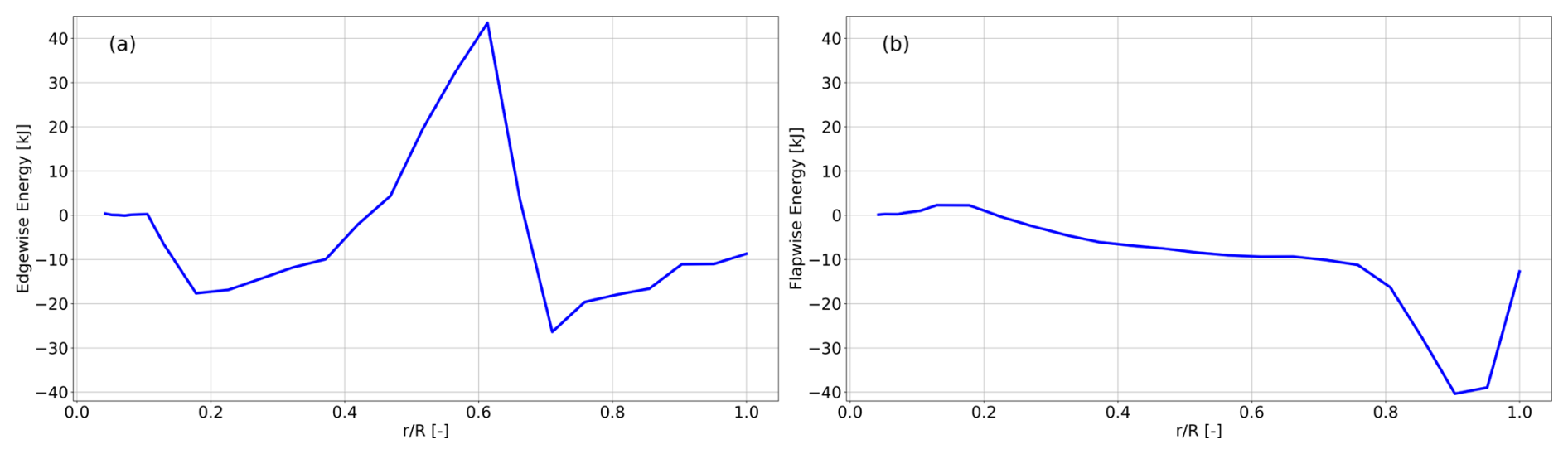
Figure 5 Energy per node of blade 2 along the blade span accumulated for the dynamic change of the yaw misalignment between −43 and −53° for (a) the edgewise direction and (b) the flapwise direction.

The flapwise accumulated energy, as shown in Fig. 5b, gives a similar pattern as for the ramp-up phase. From $r/R=\mathrm{0.2}$ outwards, all sectional flapwise energy components show negative values reaching their peak between $\mathrm{0.9}\le r/R\le \mathrm{0.95}$ and a value of −40 kJ. Over the whole blade, the flapwise aerodynamic energy sums up to −215 kJ. This means the flapwise component is being damped down during the whole investigated yawing period.

An analogous analysis of the other two blades indicates a much smaller fluid–solid energy transfer, consistently with the edgewise displacements of blade 1 (see Fig. 3d) and blade 3 (see Fig. 3f), where no vibration build up is found.

An even slower yaw rate would further amplify blade vibrations due to longer exposure to critical yaw misalignments, whereas a faster yaw rate would mitigate them. An extreme scenario would be for a blade at a fixed yaw angle within this region, which is analyzed in Sect. 3.2, where a more detailed analysis of the vibration modes is performed.

3.2 Fluid–structure interaction of the single blade

Since blade 2 exhibits significant edgewise tip vibration amplitudes during the yaw maneuver, a more detailed investigation of this blade is warranted. The rotor blades are modeled as individual cantilevered bodies, with any interaction between them occurring only through the flow field. Under this modeling approach, a single-blade analysis is expected to capture the essential physics while substantially reducing computational cost. For that purpose, Sect. 3.2.1 to 3.2.5 analyze blade 2 at fixed yaw misalignments in more detail. Two distinct scenarios are analyzed, each simulated in both rigid and flexible configurations. This approach allows for the differentiation of pure aerodynamic effects and the assessment of behavior in a fluid–structure-coupled context.

3.2.1 Aerodynamic energy transition of the full blade

To contrast situations of high- and low-blade-vibration amplitudes, single blade setups of yaw misalignments of −37 and −60° at an azimuth angle of 330° are being focused on. The first case reflects a scenario with negative aerodynamic damping, while the second case represents a clear damping period, where all vibrations have ceased (see Fig. 3e). Both cases are simulated in a rigid and flexible manner. For convenience, the four described cases are abbreviated as shown in Table 4.

Table 4 Abbreviations of the simulated single-blade cases.

An instantaneous flow field of the two yaw misalignments in rigid and flexible setups is depicted in Fig. 6, highlighting the in-plane velocity component. Figure 6a and b show the flexible and rigid simulations for a yaw misalignment of −37°, while, in Fig. 6c and d, the simulations with −60° are shown. The difference in flow structures between the two different yaw angles is apparent. Both cases with −37° show smaller structures of in-plane velocity, while the flow field with −60° inflow is described by larger structures expanding over almost the whole blade span.

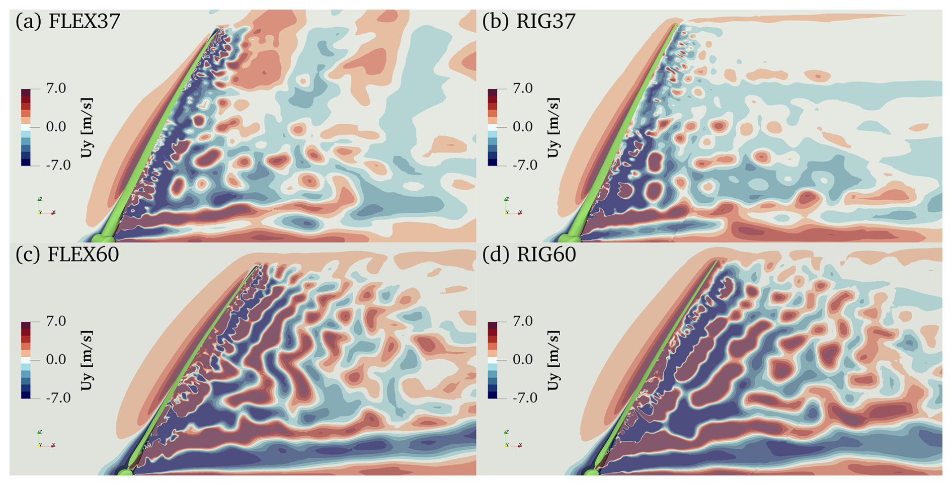
Figure 6 Instantaneous side view of the normal to plane velocity component of (a) a flexible blade at −37° yaw, (b) a rigid blade at −37° yaw, (c) a flexible blade at −60° yaw, and (d) a rigid blade at −60° yaw. A positive flow component is pointing into the plane. Blade and hub are colored in green.

At a fixed yaw angle, the edgewise, flapwise, and torsional components of the blade tip vibration of case FLEX37 are shown in Fig. 7 in the time and frequency domain. It is visible that the edgewise amplitude (Fig. 7a) reaches much higher values compared to the dynamic yaw maneuver shown in Fig. 3e as the blade stays in the critical region until it reaches a limit cycle oscillation. Here, the limit cycle is reached at 180 s, with an amplitude of 9.5 m, where the injected aerodynamic power and structural damping are balancing each other out. This is roughly 3 times the amplitude of the yawing case. From a frequency perspective, this motion is mainly dominated by the edgewise eigenfrequencies. The flapwise and torsional natural frequencies do not appear to impact the vibration behavior. This is shown in Fig. 7b, where the vertical red lines mark the blade's natural frequencies, and the second lowest corresponds to the first edgewise eigenfrequency. At this point, a slight shift in the blade's inherent oscillation frequencies towards smaller values can be noted relative to the theoretical eigenfrequencies that are based on a preceding modal analysis. This behavior is attributed to the non-linear characteristics of the blade structure, which become evident as a result of the significant deformation amplitudes. A similar behavior was also described in Abdeljawad et al. (2020). Similar findings can be observed in both the flapwise and torsional components. The flapwise component reaches an oscillation amplitude of approximately 1.7 m at a mean deflection of −5.8 m. At the limit cycle, the torsional component oscillates between −6.1 and 7.7°. Both components appear to be largely influenced by the edgewise natural frequency (see Fig. 7d and f). Consequently, the investigations will mainly focus on the edgewise component of the blade vibrations.

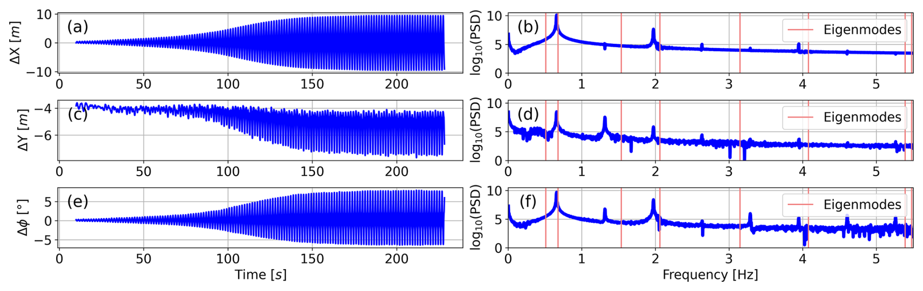
Figure 7 Vibration ramp up of the FLEX37 setup in the edgewise (a), flapwise (c), and torsional component (e). Frequency contributions of the respective components are shown in (b), (d), and (f). The vertical lines indicate the blade's eigenmodes. From low to high, the first, third, and fifth frequencies correspond to the first three flapwise eigenfrequencies, and the second, fourth, and sixth correspond to the first three edgewise eigenfrequencies. The seventh frequency represents the first torsional natural frequency.

The corresponding edgewise and flapwise energy contributions are highlighted in Fig. 8. The shape of the edgewise component in Fig. 8a deviates from the corresponding direction of the yaw maneuver in Fig. 4a. In the FLEX37 case, all analyzed sections in the range of $\mathrm{0.05}\le r/R\le \mathrm{0.95}$ contribute to an energy transition into the blade structure and therefore contribute to blade vibrations. Only the last monitored section at the blade tip does not inject power into the blade. Similar findings are described in Pirrung et al. (2024), which show that the aerodynamic energy at the blade tip changes with large vibration amplitudes relative to lower amplitudes. In the flapwise component in Fig. 8b, the deviations towards the full rotor case are even more dominant as compared to Fig. 4b. Here, positive and negative contributions of flapwise energy are being calculated for different spanwise positions, where the outer-tip part also contributes to energy injection into the blade structure. Specifically, the positive energy is concluded to act only on the amplification of the flapwise component within the first edgewise mode because a frequency analysis of the flapwise vibration component reveals contributions only from the first edgewise natural frequency and not from the first flapwise one.

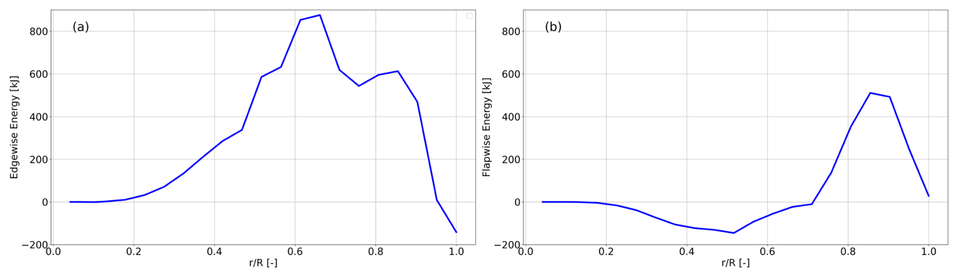
Figure 8 Energy per node of blade 2 along the blade span accumulated for case FLEX37 for (a) the edgewise direction and (b) the flapwise direction.

For comparison purposes, the edgewise blade deformation for case FLEX60 is shown in Fig. 9 in the time and frequency domain. This case can be seen as stable since the vibrations are being damped down within the investigated time period. The initial deformation peak is the result of the fluid–structure coupling being turned on at 5 s, which leads to the blade being initially deformed by aerodynamic forces and gravitational loads. From a frequency perspective, in the stable case, the first two edgewise eigenfrequencies dominate the motion. Nevertheless, other frequencies are visible in the spectral analysis, in contrast to case FLEX37.

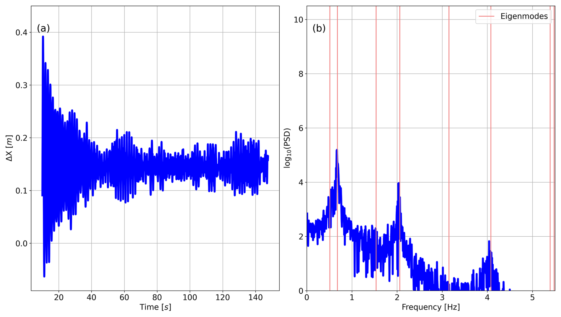
Figure 9 Edgewise vibration ramp up of the FLEX60 setup in the (a) time domain and (b) frequency domain. The vertical lines indicate the blade's eigenmodes. From low to high, the first, third, and fifth frequencies correspond to the first three flapwise eigenfrequencies, and the second, fourth, and sixth correspond to the first three edgewise eigenfrequencies. The seventh frequency represents the first torsional natural frequency.

The edgewise and flapwise aerodynamic energies over the blade span of case FLEX60 are shown in Fig. 10. For the edgewise component (see Fig. 10a) the outer 55 % of the blade contributes to aerodynamic damping since all values are negative. As the impact of the aerodynamic energy increases linearly with span, the outer part is known to be more important with respect to blade vibration analysis.

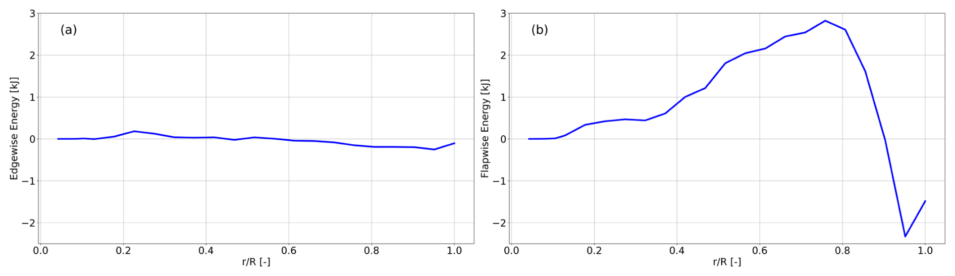
Figure 10 Energy per node of blade 2 along the blade span accumulated for case FLEX60 for (a) the edgewise direction and (b) the flapwise direction.

In conclusion, depending on the yaw misalignment configuration, i.e., −37 or −60°, the flow can either amplify or dampen the blade vibrations, underlining the importance of understanding these dynamics from both the fluid dynamics and structural perspectives. Therefore, Sect. 3.2.3–3.2.5 provide a detailed interpretation of these differences.

3.2.2 Relation of aerodynamic power and structural damping

Understanding how the aerodynamic power needs to overcome the inherent structural damping for blade excitation is essential for optimizing rotor performance and ensuring structural integrity under extreme wind conditions. Following the method of Grinderslev et al. (2022), the structural damping of the blade can be estimated from the force balance of an FSI simulation reaching a pure-mode limit cycle oscillation, where P_AERO is equal to P_STRUC. As this power is proportional to the square of the vibration amplitude, the power dissipated P_STRUC by structural damping can be described as follows:

$$\begin{array}{}\text{(8)}& P_{\mathrm{STRUC}}=C_{\mathrm{STRUC}}\cdot A^{\mathrm{2}},\end{array}$$

with A being the amplitude of the blade tip limit cycle oscillations and C_STRUC being a proportionality constant linking the dissipated power to the vibration amplitude. Assuming that the vibration of FLEX37 almost reflects the pure first edgewise mode, C_STRUC can be estimated from the last vibration cycles as follows:

$$\begin{array}{}\text{(9)}& C_{\mathrm{STRUC}}={\displaystyle \frac{P_{\mathrm{AERO}}}{A^{\mathrm{2}}}},\end{array}$$

which is, for the last 18 cycles, calculated to be 555.44 W m⁻². If, now, the difference in power between aerodynamic contribution and structural damping,

$$\begin{array}{}\text{(10)}& \mathrm{\Delta }P=P_{\mathrm{AERO}}-P_{\mathrm{STRUC}},\end{array}$$

is being plotted for blade 2 of the yaw maneuver of the full rotor (see Fig. 11), it can be seen that the blade vibrations are increasing for positive values of ΔP and are being damped for negative values for most parts of the yaw range. Based on the results shown in Grinderslev et al. (2022), one would expect the ΔP curve to start and end at 0 kW. However, in the present case, a different behavior is observed, indicating a non-zero net energy exchange at the beginning and end of the yaw maneuver. It can be noted that, for smaller vibrations in the range of −30 to −35°, increasing amplitudes are also visible even for negative ΔP values. This can be explained by the fact that, in this range, the inner part of the blade is exposed to negative aerodynamic power, while the outer part is exposed to positive aerodynamic power. In total, this gives a negative value for the whole blade, although the outer part is being excited by the flow, leading to smaller but increasing blade tip vibrations.

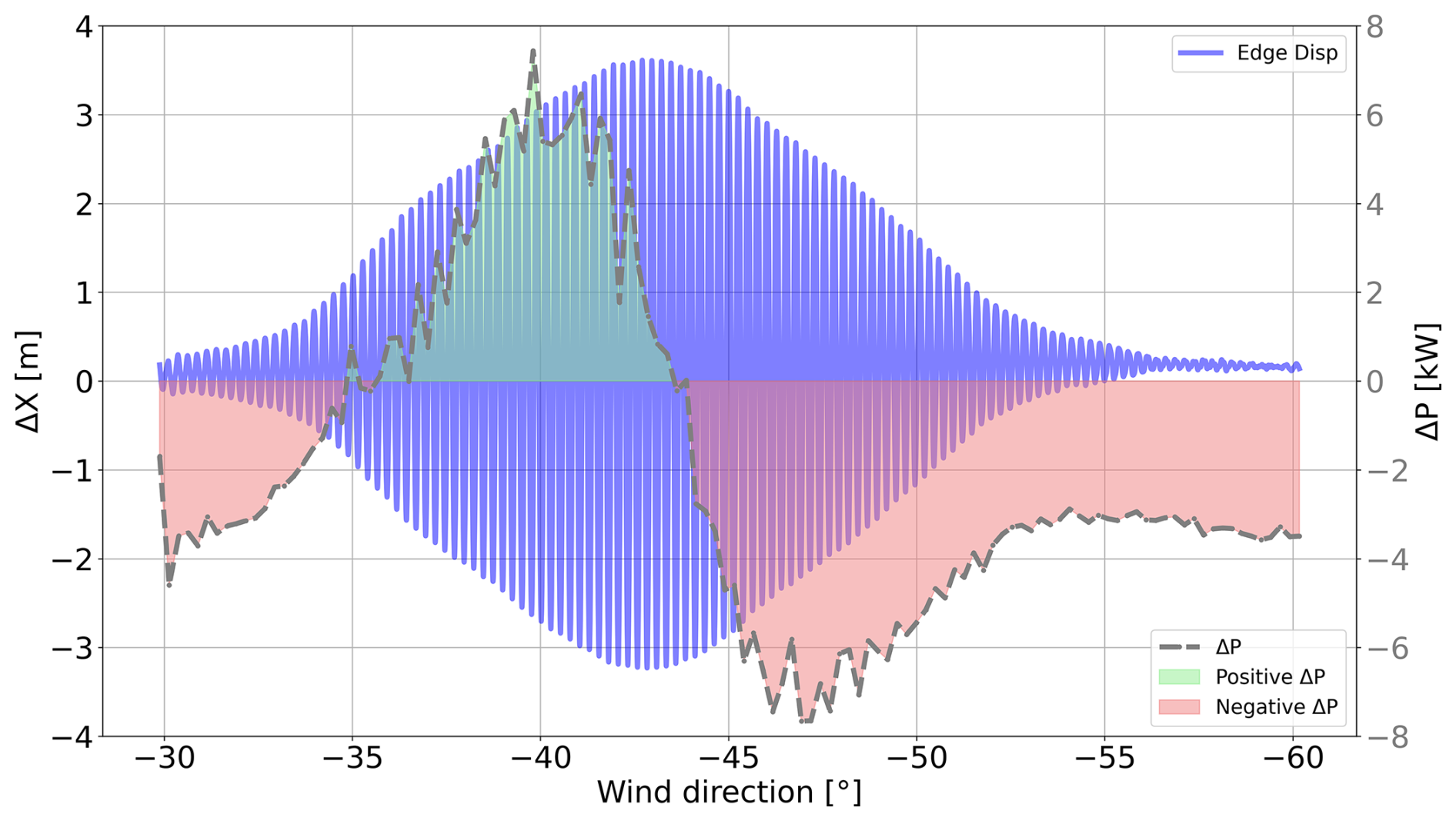
Figure 11 Blade tip displacement in edgewise direction (ΔX) for blade 2 in the range of $-\mathrm{30}\mathit{°}\ge \mathrm{Wind}\mathrm{Dir}.\ge -\mathrm{60}\mathit{°}$ (blue). The difference between total aerodynamic power and structural damping power ΔP is shown in dashed gray.

The largest ΔP that is calculated as 7.5 kW is reached at −40° in the regime of growing blade vibration amplitude. This is mirrored during the damping phase of the vibration at −47° yaw misalignment and $\mathrm{\Delta }P\approx -\mathrm{7.5}$ kW. The largest tip displacement is reached at −43°, where P_AERO and P_STRUC seem to be balanced out at ΔP≈0 kW.

3.2.3 Development of vibrations

The analysis of the integrated aerodynamic energy on the single blade in the two examined scenarios revealed that FLEX37 exhibits unstable blade vibrations, whereas FLEX60 demonstrates stability. The vibrations are primarily influenced by the first edgewise eigenfrequency, resulting in the most significant displacements at the blade tip. To gain deeper insights into the mechanisms that cause the blade to transition from standstill to either unstable or stable motion, the subsequent focus will be on examining the blade tip displacements in both cases.

In Fig. 12, the displacements of the two blade tips are illustrated. Figure 12a and b depict the motion within the horizontal x–y plane across various phases of displacement. In contrast to that, Fig. 12c and d present the edgewise component over time. The motion time series is divided into four distinct phases, each highlighted with a different color-coding. The first phase, designated as the settling phase, ranges from 6 to 20 s. It is visible that both simulation cases describe a similar motion pattern, which is mainly dominated by the coupling of fluid and structure, where the motion from the undeformed blade towards the final flapwise displacement prevails. The second phase, occurring between 20 and 40 s, is referred to as the decision phase, during which the motion may either transition to being predominantly edgewise or gradually diminish. The third phase, highlighted in dark blue, represents a typical duration of one edgewise motion cycle that takes 1.47 s. Lastly, the fourth phase extends from 41.47 to 90 s and captures the excitation of blade vibrations in the context of the unstable case, as well as the near-stabilization observed in the stable case.

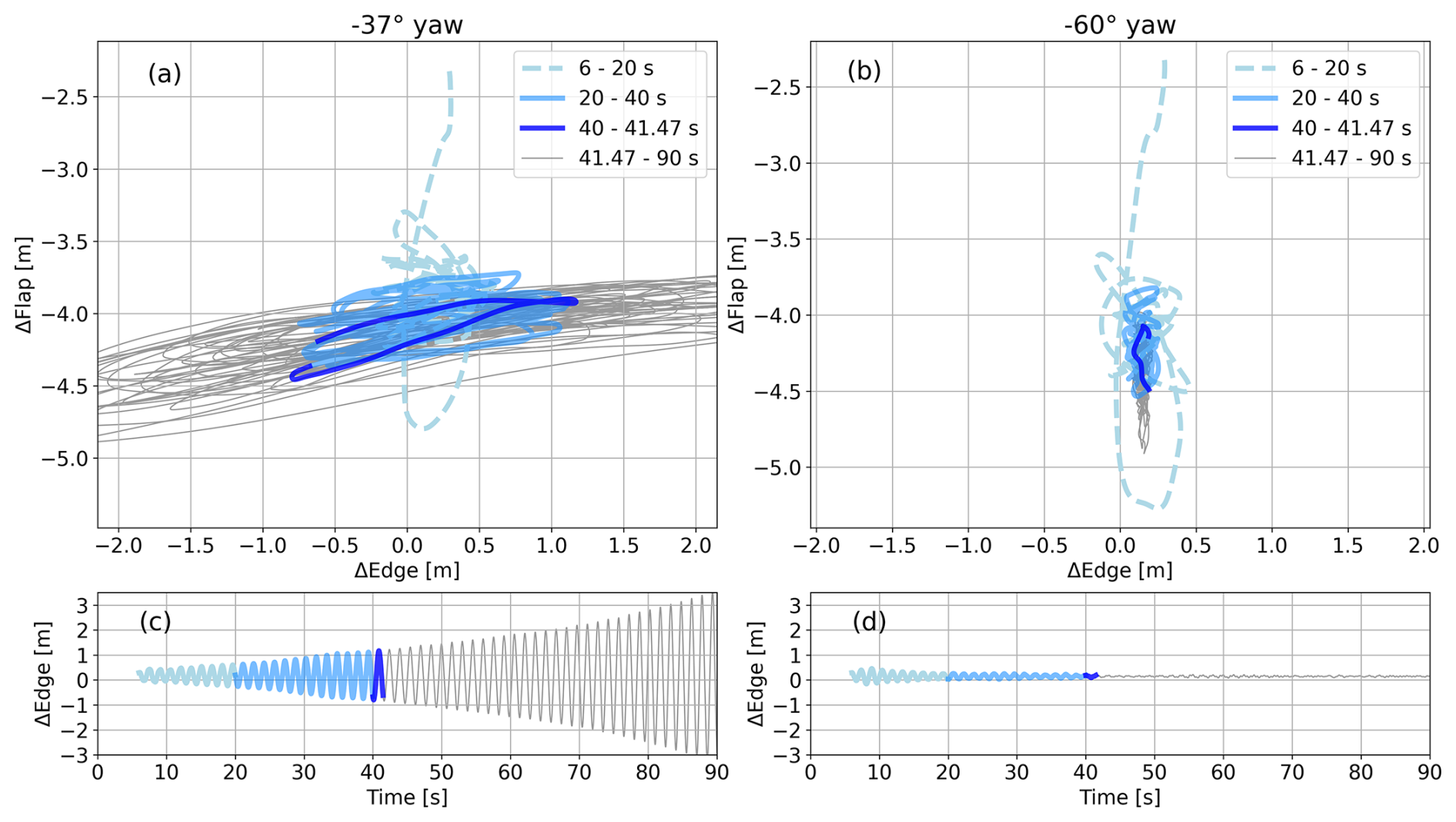
Figure 12 Blade tip displacement in edgewise and flapwise directions for (a, c) the unstable case FLEX37 and (b, d) the stable case FLEX60.

3.2.4 Characteristics of the sectional loads

The results presented illustrate the structural behavior as a result of the surrounding fluid conditions. To fully understand the interaction between structure and fluid, it is essential to analyze both aspects. To investigate the fluid side in more detail, firstly, the subsequent discussion will focus on the local inflow conditions and the corresponding sectional loads, while, secondly, fluid characteristics in the near wake are discussed in Sect. 3.2.5.

To achieve this, all four cases presented in Table 4 are examined at $r/R=\mathrm{0.9}$ since this spanwise position is expected to experience a major influence of aerodynamic energy (see Fig. 4). In this context, cases RIG37 and RIG60 represent the moment just before the settling phase begins, while cases FLEX37 and FLEX60 capture a later state during the excitation phase. Each case is analyzed over a duration of three theoretical edgewise motion cycles, amounting to 4.41 s.

Figure 13 shows the angle of attack time series of the two rigid cases using the three-point method introduced by Rahimi et al. (2018). On the one hand, for case RIG37 in Fig. 13a, the angle of attack fluctuates around −30.2° by amplitudes in the range of ±0.5°. The color-coding depicts the corresponding aerodynamic edgewise force, summed from the pressure and friction forces. Blue corresponds to a force component towards the leading edge, while red points towards the trailing edge. It is visible that, for RIG37, the edgewise force is negative throughout the whole investigated time period, ranging from 0 to −100 N m⁻¹. No connection between the small angle-of-attack fluctuations and the edgewise force is drawn. On the other hand, Fig. 13b shows the angle of attack over time for case RIG60. It is considered to be almost constant at a value of $\approx -\mathrm{55.7}\mathit{°}$, where minor changes in the predicted edgewise force of 40 N m⁻¹ are also apparent.

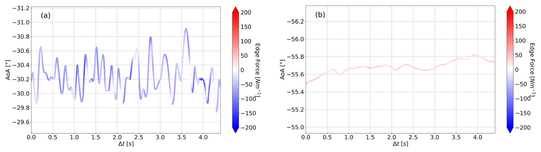
Figure 13 Time series of the angle of attack estimated using the three-point method (Rahimi et al., 2018) at $r/R=\mathrm{0.9}$ for the rigid setups (a) RIG37 and (b) RIG60.

To highlight the connection between lift and angle of attack, Fig. 14 shows the corresponding three theoretical edgewise motion cycle periods for the rigid cases RIG37 and RIG60. Here, the time is color-coded from dark blue to yellow. While the RIG37 describes a more circular pattern for the lift coefficient (C_l) values in the range of $-\mathrm{0.93}\le C_{\mathrm{l}}\le -\mathrm{0.48}$, RIG60 shows a linear increasing C_l for decreasing angle of attack and increasing time. Here, C_l values increase from $-\mathrm{0.8}\le C_{\mathrm{l}}\le -\mathrm{0.55}$.

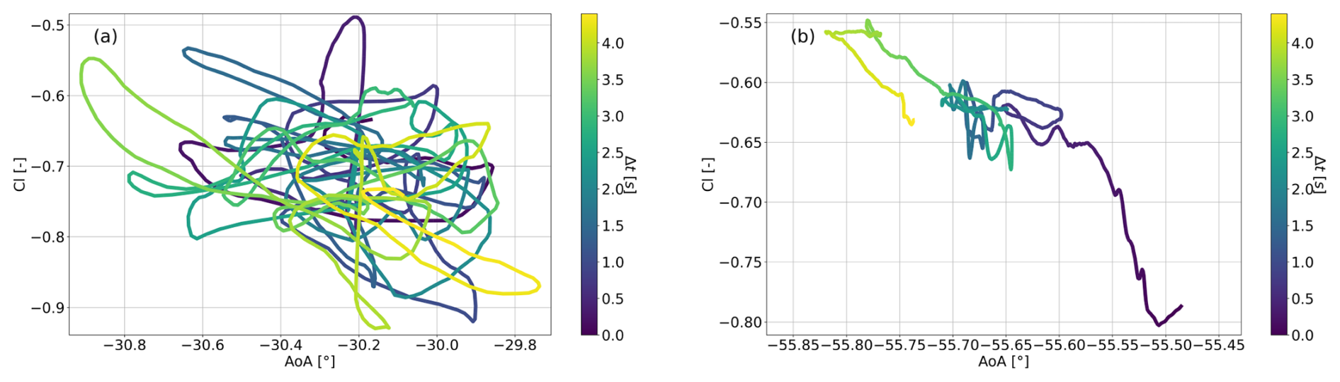
Figure 14 C_l and time over angle of attack for 4.41 s (three cycles) of cases (a) RIG37 and (b) RIG60.

Once the blade flexibility is considered and the vibration behavior reaches the excitation phase, a similar analysis is done. Figure 15 shows again the local angle of attack at $r/R=\mathrm{0.9}$ for case FLEX37 and FLEX60. It is noted that the torsional deformation also contributes to a change in angle of attack (AoA). FLEX37 shows a different behavior compared to its corresponding rigid case as it describes three distinct motion cycles that are directly reflected in terms of the angle of attack. Also, the connection between edgewise force and the angle of attack is visible. With decreasing angle of attack, the edgewise force component is found to be negative, while it flips directions when the angle of attack increases again. This change in force direction shows the contribution of the force to the direction of motion that excites the blade to vibrate. However, case FLEX60 in Fig. 15b barely differs from its corresponding rigid setup. Again, angle of attack is considered to be constant at AoA = −44° and an edgewise force of 50 N m⁻¹.

Figure 15 Time series of the angle of attack estimated using the three-point method (Rahimi et al., 2018) at $r/R=\mathrm{0.9}$ for the flexible setups (a) FLEX37 and (b) FLEX60.

Lift coefficients over time and angle of attack are shown in Fig. 16. For case FLEX37 in Fig. 16a, the circular hysteresis effect between C_l and AoA is even more pronounced. The lift describes three cycles in time that correspond to the three edgewise motion periods. This hysteresis pattern is well known and could indicate the existence of SIV and was, among others, shown in Zou et al. (2015). For the FLEX60 case in Fig. 16b, the pattern just deviates from its corresponding rigid case but still draws its linear connection, confirming that no hysteresis effect is apparent at −60° yaw.

Figure 16 C_l and time over angle of attack for 4.41 s (three cycles) of cases (a) FLEX37 and (b) FLEX60.

Thus, it is concluded that, in the case of −37° yaw misalignment, unsteady aerodynamic effects are the driving mechanism behind the vibration build-up since a hysteresis is already present in the rigid configuration. This hysteresis becomes more pronounced when blade flexibility is introduced (FLEX37), leading to lock-in with the edgewise vibration mode. This mutual influence is not evident in case FLEX60, which therefore remains stable. Because the angle of attack is extracted from velocity probes upstream and downstream of the blade, vortex shedding is inferred to make a possible contribution to the apparent vibrations, a mechanism analyzed in more detail in Sect. 3.2.5.

3.2.5 Characteristics in the near wake

To this point, blade structural deformations, as well as local aerodynamic quantities, i.e., angle of attack, lift coefficient, and edgewise force, have been studied. To understand the relation between fluid and structure, flow quantities in the near wake of the blade also have to be analyzed. For this purpose, the Hilbert–Huang transformation is used to highlight the impact of normal to inflow velocity frequencies during the different phases of the blade motion analysis. The reason for choosing this method is that, in contrast to a simple fast Fourier transformation (FFT), a clearer picture of the underlying frequency signals has been observed for various processed signals. To form a link between the local aerodynamic quantities and the near wake, this method is firstly applied on the sectional loads in contrast to the power spectrum of an FFT before investigating the near wake.

Figure 17 presents the monitored edgewise force signal for 70 s of case RIG37 at a spanwise position of $r/R=\mathrm{0.9}$, along with its corresponding frequency contributions obtained through a fast Fourier transform. The challenge of establishing a clear connection between the dominant frequencies and the force signal is evident (see Fig. 17b). The power spectrum of frequencies within the range of 0.0 Hz ≤ f ≤ 2.2 Hz appears to be uniformly distributed. No frequency stands out in the region of the first two natural frequencies. To address this issue, the Hilbert–Huang Transform is applied.

Figure 17 Edgewise sectional force signal (a) and power spectrum (b) at $r/R=\mathrm{0.9}$ for case RIG37. The vertical lines indicate the blade’s eigenmodes. From low to high, the first and third frequencies correspond to the first two flapwise eigenfrequencies, and the second and fourth correspond to the first two edgewise eigenfrequencies.

In accordance with the procedure described in Sect. 2.5, the first eight IMFs of the edgewise sectional force can be obtained from the original signal as shown in Figs. 18 and 19. A closer look on the power of the frequencies of each IMF is shown in Figs. 20 and 21. The solid lines show the power spectrum of each IMF. The dotted and dashed-dotted lines represent the first two eigenfrequencies, i.e., first flapwise and first edgewise, of the blade, respectively. According to Sect. 3.2.1, vibrations are driven by the first edgewise natural frequency. It can be seen that this frequency is already inherent in the edgewise force of case RIG37, as shown via IMF-6 (see Fig. 20a), although the blade is analyzed rigidly. In the flexible simulation (Fig. 20b), once the blade reached the excitation phase, a lock-in phenomenon of that particular frequency is visible. The whole edgewise force signal is dominated by IMF-6 in the first edgewise natural frequency, highlighting that both force and deformation are aligned in phase. Here, again, a slight shift towards the left (lower frequencies) of the natural frequency is noted. This aligns with the findings of the blade tip displacements shown in Fig. 7.

Figure 18 Intrinsic mode functions of the edgewise sectional force at $r/R=\mathrm{0.9}$ for (a) case RIG37 and (b) case FLEX37.

Figure 19 Intrinsic mode functions of the edgewise sectional force at $r/R=\mathrm{0.9}$ for (a) case RIG60 and (b) case FLEX60.

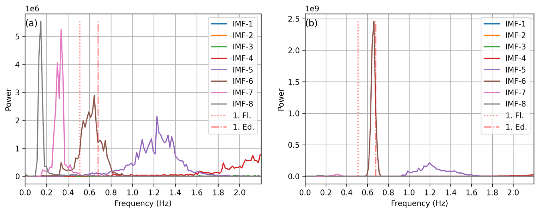
Figure 20 Power spectrum of the inherent frequencies of each IMF of the edgewise sectional force at $r/R=\mathrm{0.9}$ for (a) case RIG37 and (b) case FLEX37. The vertical lines indicate the first two eigenfrequencies of the blade, i.e., first flapwise frequency (1. Fl. – dotted line) and first edgewise frequency (1. Ed. – dashed-dotted line).

This lock-in phenomenon does not occur in the case of −60° yaw misalignment, as shown in Fig. 21. Although IMF-7 has its peak in the vicinity of the first edgewise frequency in the rigid setup (Fig. 21a), the signal's power distribution does not lock into the first edgewise natural frequency during the flexible simulation phase (Fig. 21b). It even moves further away from the frequency of scope. The slight differences between RIG60 and FLEX60 can be explained by the minor change in AoA, when the blade adjusts to the loads. This confirms the instability of FLEX37 and the stability of FLEX60 as the forces either align with the frequency of motion and contribute the vibrations or play no significant role in the ramp-up of blade vibrations being too far away from the edgewise eigenfrequency.

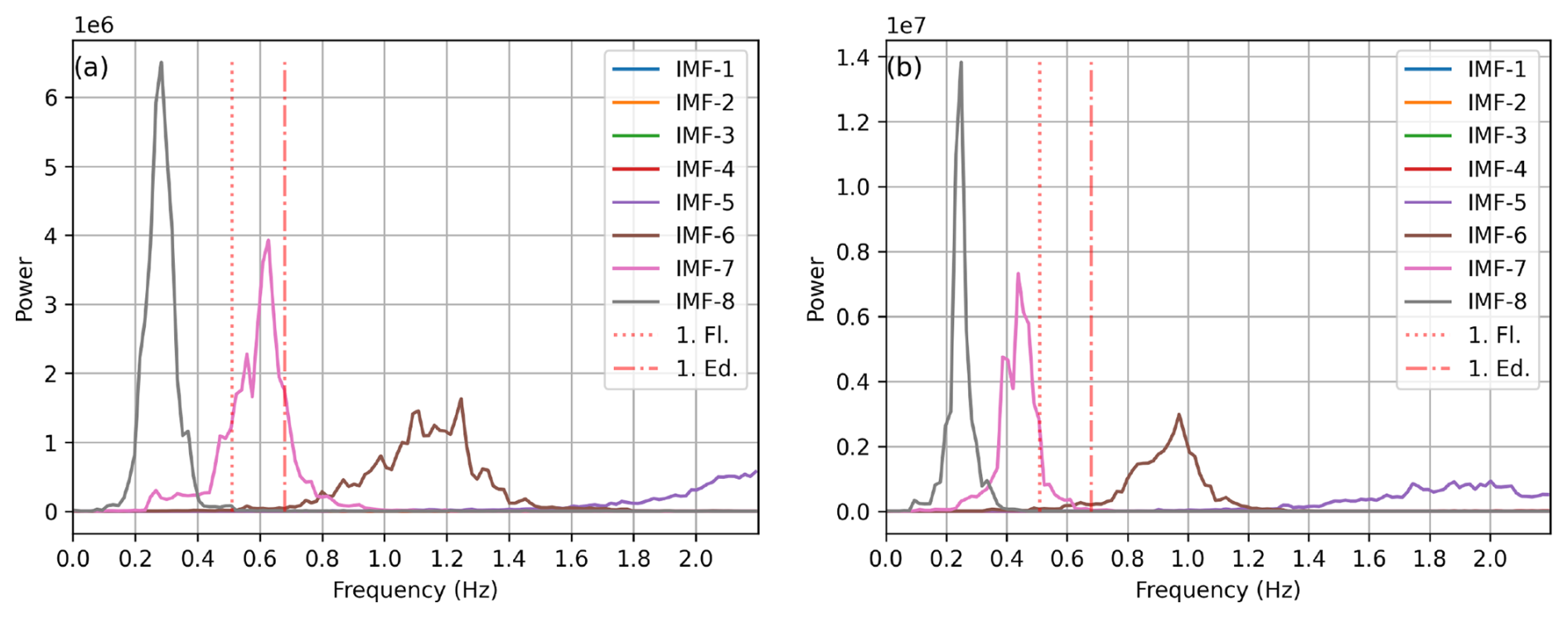
Figure 21 Power spectrum of the inherent frequencies of each IMF of the edgewise sectional force at $r/R=\mathrm{0.9}$ for (a) case RIG60 and (b) case FLEX60. The vertical lines indicate the first two eigenfrequencies of the blade, i.e., first flapwise frequency (1. Fl. – dotted line) and first edgewise frequency (1. Ed. – dashed-dotted line).

To see a similar frequency impact on the flow in the wake of the blades, the HHT is applied to the v velocity component that is pointing horizontally, normal to the inflow direction. For that purpose, a velocity probe is analyzed, located three chord lengths downstream of the $r/R=\mathrm{0.9}$ position. A probing rate of 10 Hz is used to save computational costs and focus on frequencies within 0.0 Hz ≤ f ≤ 2.2 Hz. Figure 22 shows the impact of this frequency range on the probed velocity signal for the two rigid setups, RIG37 and RIG60. Even more pronounced than in the investigated sectional force signal, case RIG37 consists of a dominant frequency component in the near wake at the edgewise eigenfrequency, as shown by IMF-3 in Fig. 22a. Additionally, frequencies around 1.5 Hz show larger relative power peaks compared to the sectional loads. On the other hand, Fig. 22b shows the corresponding velocity frequency spectrum for the RIG60 case. It is visible that the edgewise frequency component makes a minor contribution to the frequency–power distribution of the velocity signal in contrast to the wide spread of IMF-1, which dominates the velocity component.

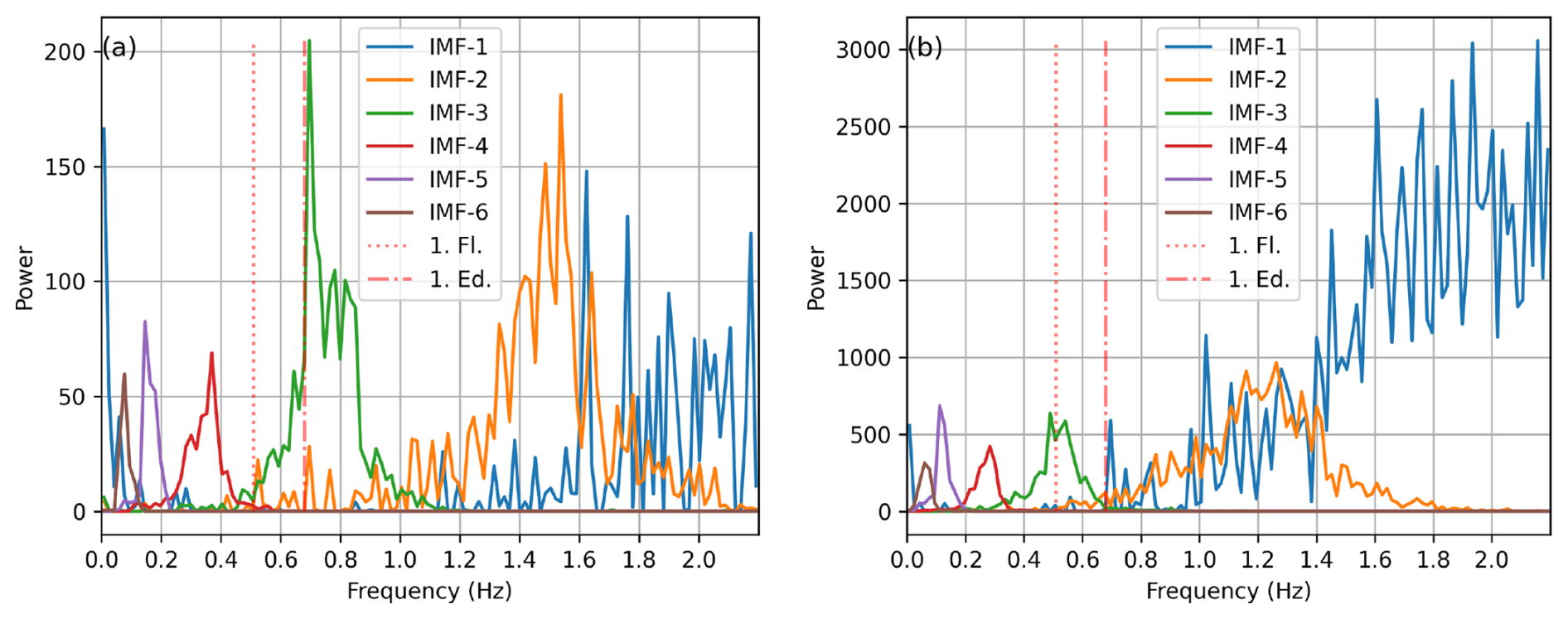
Figure 22 Power spectrum of the inherent frequencies of each IMF of the flow velocity component v at $r/R=\mathrm{0.9}$ for (a) case RIG37 and (b) case RIG60. The vertical lines indicate the first two eigenfrequencies of the blade, i.e., first flapwise frequency (1. Fl. – dotted line) and first edgewise frequency (1. Ed. – dashed-dotted line).

For the two flexible cases, FLEX37 and FLEX60, the investigation is again split into the three time periods, i.e., the settling phase, the decision phase, and the excitation phase. Firstly, Fig. 23 shows the frequency–power distribution for the settling phase. As this case is seen as the transition from rigid towards flexible setups, it can be seen in Fig. 23a that, especially for the FLEX37 case, most frequency components in the vicinity of the first two natural frequencies are being damped out. This can be explained by the drag-driven deformation trajectory described in Sect. 3.2.3 that does not allow for periodic repetitions of deformations.

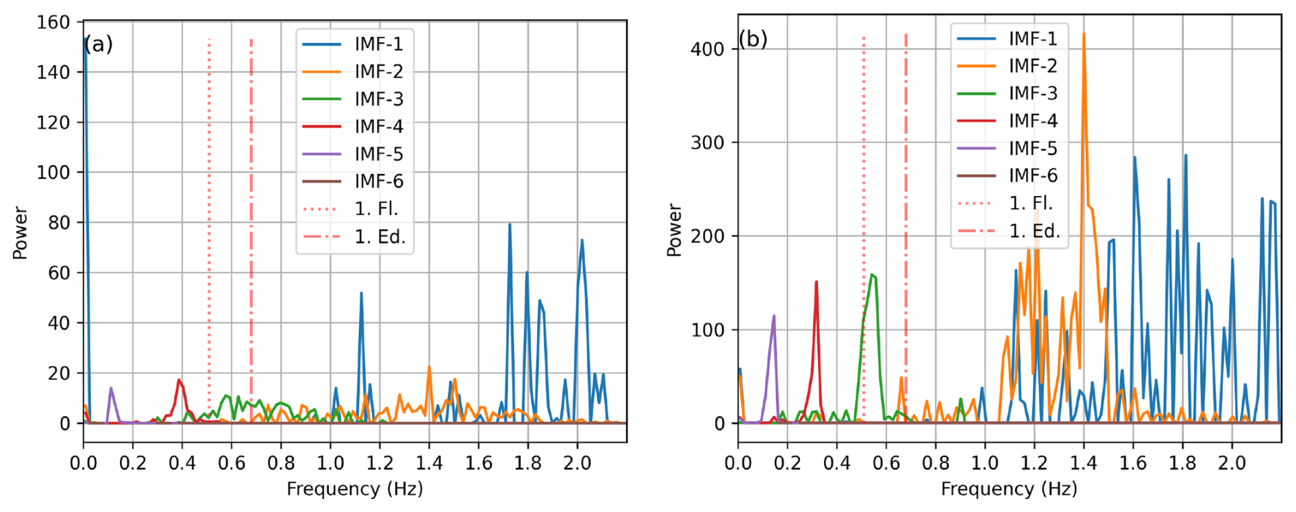
Figure 23 Power spectrum of the inherent frequencies of each IMF of the flow velocity component v at $r/R=\mathrm{0.9}$ for (a) case FLEX37 and (b) case FLEX60 from 0 to 20 s. The vertical lines indicate the first two eigenfrequencies of the blade, i.e., first flapwise frequency (1. Fl. – dotted line) and first edgewise frequency (1. Ed. – dashed-dotted line).

Within the decision phase, flow characteristics seem to have adjusted towards the given blade deformation conditions and, in the case of FLEX37, feed back with aeroelastic frequencies at the blade by showing increasing impact of the first edgewise frequency (see Fig. 24a). However, this is not the case for FLEX60, where frequencies barely move closer to the edgewise eigenfrequency, as shown in Fig. 24b.

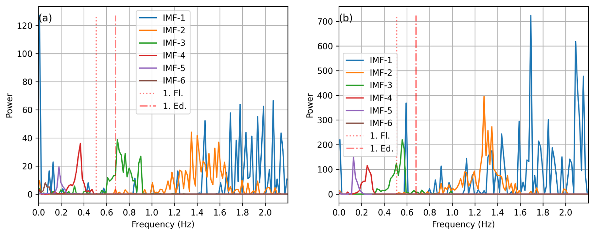
Figure 24 Power spectrum of the inherent frequencies of each IMF of the flow velocity component v at $r/R=\mathrm{0.9}$ for (a) case FLEX37 and (b) case FLEX60 from 20 to 40 s. The vertical lines indicate the first two eigenfrequencies of the blade, i.e., first flapwise frequency (1. Fl. – dotted line) and first edgewise frequency (1. Ed. – dashed-dotted line).

Within the excitation phase in Fig. 25, the picture becomes more clear. Case FLEX37 clearly locks-in on the edgewise eigenfrequency at 0.68 Hz, while FLEX60 only shows a minor peak at this particular frequency compared to the whole given frequency power distribution.

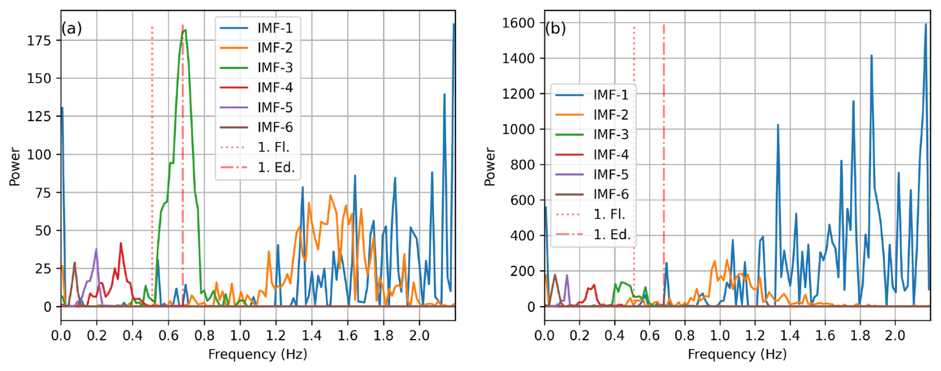
Figure 25 Power spectrum of the inherent frequencies of each IMF of the flow velocity component v at $r/R=\mathrm{0.9}$ for (a) case FLEX37 and (b) case FLEX60 from 40 to 90 s. The vertical lines indicate the first two eigenfrequencies of the blade, i.e., first flapwise frequency (1. Fl. – dotted line) and first edgewise frequency (1. Ed. – dashed-dotted line).

In summary, case FLEX37 exhibits large edgewise vibration amplitudes, in contrast to the stable FLEX60 case. This difference arises from the frequency contribution near the first edgewise eigenfrequency already present in the rigid setup, RIG37, whereas RIG60 is driven by components around 2 Hz. In Fig. 6c and d, it can be seen that the wakes of RIG60 and FLEX60 are dominated by strongly correlated structures. As shown by Heinz et al. (2016), such correlated shedding can be triggered by inclined inflow at specific inflow angles, which seems to apply here as well.

Using a characteristic vortex shedding Strouhal number for wind turbine blades at high angles of attack of Sr = 0.15 (see Heinz et al., 2016; Skrzypiński et al., 2013), an inflow speed of 35 m s⁻¹, and the observed shedding frequency of f=2 Hz in FLEX60, the characteristic blade length can be calculated as follows:

$$\begin{array}{}\text{(11)}& L={\displaystyle \frac{\mathit{Sr}\cdot U}{f}}=\mathrm{2.6}\mathrm{m}.\end{array}$$

It corresponds to the chord lengths in the spanwise range of $\mathrm{0.8}\le r/R\le \mathrm{0.9}$, the region that is primarily responsible for the injected aerodynamic power (see Figs. 8a and 10a). In Heinz et al. (2016), these correlated structures were created from inflow speeds that produced shedding near the edgewise eigenfrequency, leading to large blade vibrations. Here, however, opposing behavior can be observed. The dominant correlated frequencies are roughly 3 times higher than the first edgewise mode due to the much higher inflow speed of 35 m s⁻¹. Consequently, the dominating wake correlation appears to stabilize the blade by washing out frequency contributions near the first edgewise frequency. A preceding study showed that a FLEX60 setup with a uniform inflow velocity of one-third of the original speed, i.e., 11.77 m s⁻¹, could indeed trigger small vibrations (slightly larger amplitudes than in the original FLEX60) in the pure first edgewise eigenmode. However, the lack of growth to larger amplitudes was attributed to insufficient energy in the flow. Although the critical vortex shedding frequency was met, the fluid did not transfer enough energy to overcome structural damping.

It is therefore concluded that instability occurs when wake structures lock in with the first edgewise eigenfrequency (FLEX37), whereas higher-frequency correlated wake shedding that avoids this lock-in suppresses energy near the mode and stabilizes the blade (FLEX60). In the FLEX37 case, the observed coherent wake frequencies cannot be attributed to classical Strouhal shedding from a bluff body. Instead, the instability appears to originate from a three-dimensional separated shear layer that develops under yawed and inclined inflow, generating periodic wake structures whose characteristic frequency approaches the first edgewise eigenfrequency. This frequency alignment promotes lock-in and results in negative aerodynamic damping.

4 Conclusion and outlook

This study presents an approach for predicting blade vibrations of multi-megawatt wind turbines in a storm fault scenario, where one blade is assumed to fail to pitch to feather and remain at a −60° pitch angle and where the rotor is deliberately yawed so that the inflow impinges from the side and the mean loads are minimized. Using isolated blades and progressing from rigid models to fully fluid–structure-coupled simulations, the onset of vibrations and the lock-in of wake structures with the first edgewise structural frequency is investigated, thereby uncovering unwanted side effects of this load alleviation maneuver. The approach is directly relevant to the simulation of extreme load cases, enabling more accurate prediction of peak aeroelastic loads and lock-in behavior under yawed inflow, and it can support the inclusion of critical rotor–inflow conditions in future controller design.

The investigation of the yaw maneuver from 0 to −90° of the full rotor at a constant yaw speed revealed that the blade pointing upward with an inclination angle that results in spanwise flow from root to tip experiences vibrations within a specific range of yaw misalignment angles. The vibration ramp-up is driven by energy transfer from the fluid into the blade structure, primarily occurring in the outboard region. Beyond a certain yaw angle, amplitudes decrease as energy is dissipated back from the blade into the fluid. It is noted that even with negative total effective power ΔP, vibration growth can start due to outboard excitation and inboard vibration damping. However, instabilities grow rapidly once the effective power becomes positive near −35° yaw misalignment and diminish near −43°, where the blade stabilizes for the turbine under investigation. Additionally, the present work can be seen as an alternative approach to mapping the influence of inflow angles on a given turbine blade, complementing the study of Horcas et al. (2022), by continuously varying the inflow angle at constant inclination and thereby identifying regions of elevated vibration risk when the time spent in these critical conditions is sufficient to modify the blade’s vibration state. A direct comparison of the results with those for the smaller blade in Horcas et al. (2022) is, however, difficult because, although the first edgewise frequencies of both blades are very similar, the inclination angle in this study (−30°, flow from root to tip) lies well outside the range considered for the smaller blade (0 to 70°, flow from tip to root).

At a fixed yaw, stable (FLEX60) and unstable (FLEX37) situations revealed that, in the case of the unstable situation, a force lock-in near the first edgewise eigenfrequency leads to the rapid tip deformation, which could also be confirmed by its C_l vs. AoA hysteresis. No such lock-in effect could be found for the stable case. It is revealed that, in the unstable situation, the wake also locks in with the blade motion, whereas, in FLEX60, the Strouhal-driven correlated vortex structures dominate the wake with frequencies far from the critical regime, preventing instability. This Strouhal-type shedding is absent in the case of FLEX37, likely due to different inflow conditions, which is consistent with the findings of Horcas et al. (2022), where, at low inclination angles, the wake is mainly described by generalized shedding. Overall, vibration stability is found to be case (and turbine) specific, occurring only when inflow speed, inclination angle, and the blade's edgewise eigenfrequency align.

Although slower than pitching, yawing the turbine proved to be effective in guiding the system to a stable state while reducing vibration amplitudes to roughly half its magnitude and thus offers a mitigation possibility when a fast pitch movement is restricted. Providing it is mechanically feasible, an even faster yaw rate could further reduce the vibration amplitude by shortening the exposure time to the critical region. If this is not possible, this approach could provide an assessment of the additional loads acting on the rotor. Therefore, the design process of turbines of this size should account for inflow-dependent blade oscillations by mapping critical regimes via coupled CFD–FSI simulations, if possible, and tuning the edgewise blade stiffness and outboard damping while ensuring a robust pitch and yaw control validated against extreme load cases.

Future research should adopt a multi-body structural approach to account for interactions among structural components of the rotor that would impact the global turbine response. Including the tower, while aerodynamically negligible in a locked-azimuth configuration, would strengthen the structural fidelity. Implementing an advanced turbine controller may enhance the operational response of the turbine. Further investigation should also address the influence of turbulence and its interaction with wake structures on blade vibrations as this enhances the physical depth of the problem.