Mountain wave and downslope winds impact on wind power production

Vertically propagating mountain waves, accompanied by strong downslope winds, occur frequently along the coast of Norway and cause accelerated surface winds on the lee side and downstream of the mountain. Mountain waves form when stably stratified air flows over a mountain and can potentially impact the power production in wind parks located in complex terrains. Although mountain waves and downslope windstorms have received significant attention within the meteorology community, they have received less focus within the wind energy industry. Taking advantage of wind and power production data from a grid of 67 wind turbines spread across two nearby mountains, this study documents accelerated wind speeds and enhanced power production on the lee side of the mountains compared to the mountain crest. The result of this study suggests that considering mountain waves in the planning phase of future wind parks may allow for an optimal layout of the wind turbines and improve profitability. The non-dimensional mountain height, $\widehat{H}$, is a key parameter for describing the development of mountain waves, and this study finds a strong relationship between $\widehat{H}$ and the accelerated downslope winds. The results of this study suggest that mountain-wave-induced accelerated downslope winds tend to occur in the wind park when $\widehat{H}<\mathrm{3}$; above this value, the lee side wind tends to be weaker than at the mountain crest. Finally, the Weather Research and Forecasting model reproduces the spatial variations in the wind speeds within the two wind parks relatively well during periods of strong downslope winds. However, the differences in the wind speeds at the windward side, the mountain top, and the lee side are not as pronounced as in the observations.

1 Introduction

Onshore wind energy, as one of the most cost-effective renewable electricity sources, will play a key role in decarbonisation, and rapid global growth is anticipated (Abdelilah et al., 2024). With nearly 25 % of the continental areas of Earth being in mountainous terrain (Zhao and Li, 2015), increasing the knowledge of how wind power production can be affected by terrain-induced wind patterns is crucial to maintain and further reduce the cost of wind energy (Veers et al., 2019). Mountain waves occur in mountainous areas all over the world (Klemp and Lilly, 1975). Along the Norwegian rugged coastline, with mountain tops, ridges, and steep slopes, mountain waves are frequently reported (Sandvik and Harstveit, 2005; Wagner et al., 2017). This research addresses mountain-wave-induced strong downslope winds on the lee side of the mountain and its impact on wind power production. A better understanding of how wind power production can be affected by the mountain wave phenomenon is important to ensure an optimal layout of future wind parks and to improve power production forecasts.

Mountain waves can form when stably stratified air flows over a mountain barrier (Holton and Hakim, 2013). Stably stratified air resists vertical movement, and when air is forced over a mountain, buoyancy forces act to restore the air to its equilibrium position. The wave created might be evanescent, but it can also propagate far downwind or high up into the atmosphere with increasing amplitude (Holton and Hakim, 2013). Depending on the characteristics of the mountain waves, wind farms can be affected in several ways. Horizontally propagating mountain waves, also known as lee waves, can affect the power production in wind parks far downstream of the mountain barrier. Stationary or nearly stationary lee waves with a long wavelength can lead to high or low power production at several wind parks simultaneously, while shorter-wavelength lee waves can affect power production at a single wind park or even just a few turbines within a wind park (Draxl et al., 2021). Vertically propagating mountain waves may be accompanied by strong downslope winds (Durran, 1990), creating favourable wind speeds for power production on the lee side of the mountain. Given the right conditions, these accelerated downslope winds can be two to three times stronger than the wind speeds at the mountain top (Jackson et al., 2013). Strong downslope winds can also cause strong wind gusts and turbulence (Klemp and Lilly, 1975) that can alter wind power production and reduce the lifetime of wind turbines (Kosović et al., 2025). In addition, the accelerated downslope winds can terminate in a hydraulic jump accompanied by rotor development, further reinforcing the turbulence, and can potentially lead to locally reversed airflow downstream of the lee side of the mountain (Doyle et al., 2000; Doyle and Durran, 2007; Gaberšek and Durran, 2004).

Strong downslope winds can form when a critical layer exists above the mountain that reflects parts of the wave energy back down to the lower parts of the atmosphere (Durran, 1990; Klemp and Lilly, 1975). A critical layer is a layer in the atmosphere where the wind changes in such a way that the cross-barrier flow becomes zero or reversed (Metz and Durran, 2023). A critical layer can also be induced locally when vertically propagating waves with increasing amplitude become unstable and break above the mountain barrier (Durran, 1990). Conditions favouring increasing amplitude and wave breaking, such as a decrease in air density and reduced wind speed with altitude, are well described in the literature (e.g. Sharman et al., 2012; Durran, 2003). A third theory describing the mechanism of downslope windstorms is based on hydraulic theory and shallow-water equations (Jackson et al., 2013). Downslope windstorms occur when subcritical upstream flow becomes supercritical over the mountain crest and accelerates down the lee slope. Further downstream, the energy is dissipated in a hydraulic jump where the subcritical conditions are restored.

Known for causing extensive wind damage, triggering aviation hazards, and exacerbating the spread of wild fires, downslope windstorms have received significant attention from the meteorology community over several decades (Smith, 1985; Durran, 1990; Mobbs et al., 2005; Smith and Skyllingstad, 2011; Rögnvaldsson et al., 2011; Metz and Durran, 2023). Within the field of wind energy, downslope winds, and mountain waves in general, have received less attention (Kosović et al., 2025). According to Wilczak et al. (2019), the impact of mountain waves on wind power production was documented for the first time during the Second Wind Forecast Improvement Project. Subsequent studies based on the same datasets further studied the mountain lee wave impact on power production (Draxl et al., 2021; Xia et al., 2021). Draxl et al. (2021) documented large oscillations in power production due to mountain waves, corresponding to 11 % of the rated power of a wind park located downstream of the Cascade Range in the Pacific Northwest of the United States. Sherry and Rival (2015) linked downslope windstorms to potential wind power ramps 50 km downwind of the Rocky Mountains in Alberta, Canada. The Perdigão field campaign in Portugal addresses wind flow processes in complex terrain relevant for wind power production, including mountain waves (Fernando et al., 2019). Radünz et al. (2021) studied how a range of static-stability conditions affected power production at two wind farms in Brazil situated on a plateau. The study concluded that wind turbines on the leeward side of a plateau tend to have higher power production compared to turbines on the windward side under stable atmospheric conditions.

While previous studies have focused on lee waves and wind energy production (Xia et al., 2021; Draxl et al., 2021), this paper focuses on wind power production under the influence of vertically propagating waves accompanied by strong downslope winds. To the knowledge of the authors, there are no previous studies addressing this issue. This study is based on a dataset of wind observations and power production collected from an array of 67 wind turbines covering two nearby mountains. The dataset allows for documentation of the spatial variation in hub height wind speeds and turbine performance within the wind park during events of mountain-wave-induced downslope winds, as well as periods where the wind speed is lower on the lee side of the mountain than on the mountain top.

Secondly, this study evaluates the ability of the Weather Research and Forecasting (WRF) model (Skamarock et al., 2019) to reproduce mountain waves and downslope winds, as well as hub height wind speeds and power production, during these events. Within the wind industry community, numerical weather prediction (NWP) mesoscale models, in particular the WRF model, are frequently used for research purposes, wind energy assessments, and forecasts (Byrkjedal and Berge, 2008; Fernández-González et al., 2018; Davis et al., 2023; García-Santiago et al., 2024). NWP models offer estimates of the wind field over large areas, including spatial and temporal variations, and are capable of reproducing hub height wind features in complex terrain (Carvalho et al., 2013; Solbakken et al., 2021; He et al., 2023). The WRF and other mesoscale NWP models have also successfully been employed to model various types of mountain waves on different scales, as well as downslope windstorms (Doyle et al., 2000; Sandvik and Harstveit, 2005; Rögnvaldsson et al., 2011; Wagner et al., 2017; Silver et al., 2020; Xia et al., 2021; Draxl et al., 2021; Samuelsen and Kvist, 2024).

In addition, taking advantage of this rather unique dataset, this study delves into the relationship between the non-dimensional mountain height, $\widehat{H}$, and the observed accelerated wind speeds on the lee side of the mountain. Whether or not mountain waves will form and break depends on factors such as the potential energy required for the flow to pass over the barrier and the kinetic energy available in the airflow. The non-dimensional mountain height represents the ratio of these factors, and within the meteorology community, $\widehat{H}$ is recognised as a key parameter for describing the development of mountain waves (Smith, 1989; Jackson et al., 2013). Numerical studies, based on internal gravity wave theory, of flows with uniform wind speed and stratification have shown that the non-dimensional parameter, in combination with the aspect ratio of the mountain, is sufficient to determine the likelihood of a cross-barrier flow to break aloft and create accelerated wind speeds on the lee side (Smith, 1985; Gaberšek and Durran, 2004). This study evaluates whether a similar relationship exists between $\widehat{H}$ and the accelerated downslope winds observed within the wind park. If such a relationship exists, the non-dimensional metric could be valuable to the wind energy community. Combined with pre-development wind measurements, $\widehat{H}$ would indicate whether winds are more likely to be diverted around the mountain, resulting in a wake formation on the lee side with low wind speeds and eddy formation due to upstream blocking, or if the flow is more likely to pass over the mountain (Baines and Smith, 1993). In the operation phase, $\widehat{H}$ could indicate whether to expect enhanced power production on the mountain lee side.

The remainder of this paper is structured as follows. Section 2 describes the study area, the observational data, the methods of this study, and the configuration of the WRF model. Section 3 includes the results and the discussion, as well as two case studies. A summary of our findings is given in the conclusion in Sect. 4.

2 Data and methods

2.1 Study area and observations

Wind observation and power production data have been collected from two wind parks, wind park A and wind park B, located on the large island Kvaløya in northern Norway. Figure 1 shows the location of the wind parks and the surrounding terrain. The topography in the surrounding area is characterised by fjords, straits, and islands, as well as mountains, with elevations ranging from sea level (brown) up to 1800 m above sea level (m a.s.l.) (light blue). The prevailing wind direction in the wind parks is from the southeast (SE), and the observed yearly mean wind speed, prior to the wind park development, was 7.86 and 7.39 m s⁻¹ at 80 m above ground level (m a.g.l.) at A and B, respectively (Solbakken et al., 2021). The SE wind direction is particularly common during the winter months, when the cold inland climate and relatively warm North Atlantic Ocean current give rise to a pressure gradient in the east–west direction and a strong land breeze (Grønås and Sandvik, 1998). In addition, during winter, high-pressure systems building up over land, in combination with low-pressure systems frequently present over the North Atlantic Ocean (Solbakken et al., 2021), can further reinforce the pressure gradient and the wind field. Mountain waves are expected to occur more frequently during the winter months, when the stability in the lower part of the atmosphere is typically relatively strong at these latitudes (Boy et al., 2019). Stably stratified air, approaching the coast from the east and southeast, will be affected by the topography and form complex wind patterns such as wakes, gap winds, mountain waves, and strong downslope winds (Samuelsen, 2007). The operator of the wind parks frequently experiences strong winds on the lee side of the mountain during periods of wind from the SE, although this has not yet been documented scientifically (Andreas Schmid, personal communication, 2021).

.

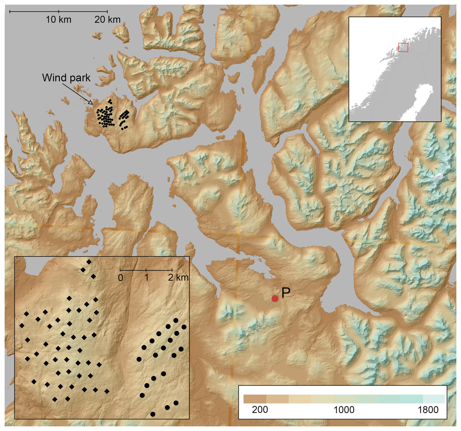
Figure 1 The location of the wind turbines (black dots) included in this study (wind parks A and B) and the surrounding terrain elevation, ranging from sea level (brown) to about 1800 m a.s.l. (light blue). The map is based on the basic nationwide digital terrain model, with a 10 m resolution, distributed by the Norwegian Mapping Authority. The red dot indicates the location P where the ERA5 data are retrieved. The inserted map in right-hand corner shows the land area (grey) and the ocean (white) of the northern Scandinavian Peninsula. The red rectangle outlines the area of the larger map. The inserted map in the lower-left corner is a zoomed-in figure of the wind turbines in wind parks A (diamonds) and B (squares)

Figure 2 shows a close-up view of the wind parks and the topography, with dark green indicating sea level and yellow indicating altitudes up to 560 m a.s.l. The black dots and squares indicate the locations of the wind turbines that in total cover an area of approximately 7 km × 7 km. Wind park A (dots) consists of 47 wind turbines, evenly distributed over the mountain at elevations ranging from 300 to 557 m a.s.l. Wind park B (squares) consists of 20 turbines distributed in row-like formations at elevations ranging from 359 to 514 m a.s.l. The wind turbines are of the type Siemens SGRE-DD-130, with a rotor diameter of 130 m, a hub height of 85 m a.g.l., and a rated capacity of 4.2 MW. Observation data with a 10 min resolution between 4 September 2020 and 24 January 2021 have been used in this study, including wind speed and wind direction taken at hub height, as well as the power production from each turbine.

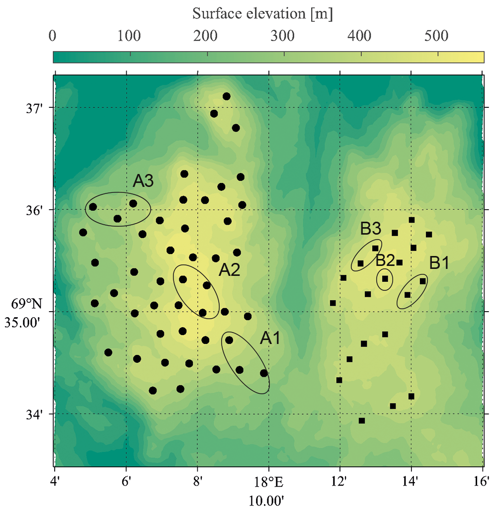
Figure 2 The topography and the locations of the wind turbines within wind park A (black dots) and wind park B (black squares). The ellipses mark the turbine clusters located upstream of the mountain tops (A1 and B1), on the mountain tops (A2 and B2), and downstream of the mountain tops (A3 and B3) during SE events. The map is based on the basic nationwide digital terrain model with a 10 m resolution, distributed by the Norwegian Mapping Authority.

In order to study how these particular wind parks are affected by mountain waves, only hub height winds from the SE are considered, more specifically wind from the 120–165° sector. This is the prevailing wind direction in the wind park and the direction from which strong downslope winds are expected to occur frequently. The selection of time slots where the wind comes from the SE is based on the observations at the turbines and is referred to as SE events. For a time period to be considered an SE event, the wind direction observed at 40 turbines or more must be within the selected wind sector. In addition, only periods that last for more than 4 h are considered, and if a period lasts for more than 48 h, the first 24 h is considered to be a separate event.

The marked areas in Fig. 2 show selected clusters of wind turbines that, under SE wind directions, are located upstream of the mountain top (A1 and B1), at the mountain top (A2 and B2), and downstream of the mountain top (A3 and B3). For the purpose of this study, the mean values of the wind speed, wind direction, and power production of each turbine cluster are considered. By evaluating the mean values of the wind turbines within each cluster, instead of values from single turbines, the impact from small local topographic effects is reduced. In the case studies in Sect. 3.4.1 and 3.4.2, wind and power data from each of the 67 turbines of the wind parks are included.

2.2 Evaluation of upstream atmospheric conditions

The formation and development of mountain waves depend on the atmospheric conditions upstream of the mountain. In order to evaluate the state of the atmosphere upstream of the study location, and as an alternative to in situ observations, meteorological parameters have been retrieved from the fifth-generation atmospheric reanalysis (ERA5) provided by the European Centre for Medium-Range Weather Forecasts (ECMWF) (Hersbach et al., 2020). The global reanalysis is produced by combining weather observations with numerical weather prediction modelling. With a spatial resolution of approximately 31 km and hourly output, ERA5 provides detailed information on the evolution of the atmosphere. Relevant meteorological parameters at the 137 vertical model levels of ERA5 have been retrieved at the model grid point location indicated by a P in Fig. 1.

The Scorer parameter indicates how a mountain wave develops depending on the atmospheric stability and the wind speed and is given by the following equation:

$$\begin{array}{}\text{(1)}& l(z{)}^{\mathrm{2}}={\displaystyle \frac{N(z{)}^{\mathrm{2}}}{U(z{)}^{\mathrm{2}}}}-{\displaystyle \frac{\mathrm{1}}{U\left(z\right)}}{\displaystyle \frac{d^{\mathrm{2}}U\left(z\right)}{d{z}^{\mathrm{2}}}},\end{array}$$

where the Brunt–Väisälä frequency N(z) and the wind speed U(z) are a function of the altitude z. The Scorer parameter is calculated at each ERA5 model level. The horizontal wind speed is decomposed such that only the wind speed in the SE wind direction of 135° is considered and is referred to as the tangential wind speed. For simplicity, the curvature term has been omitted in the calculations, so $l\left(z\right)\approx N\left(z\right)/U\left(z\right)$. When the Scorer parameter l decreases strongly with height, the formation of trapped lee waves can be expected (Jackson et al., 2013). Favourable conditions for vertically propagating mountain waves are found when l is nearly constant with height. A Scorer parameter that increases with height indicates conditions allowing for the mountain wave amplitude to grow until breaking occurs. If l increases abruptly with height, as when the cross-barrier flow becomes zero, or reversed, a critical layer exists where vertically propagating mountain waves can be absorbed and reflected, causing strong downslope winds.

Another parameter frequently used to describe the development of mountain waves is the non-dimensional mountain height denoted $\widehat{H}$. This parameter combines the cross-barrier wind speed U, the mountain height h₀, and the stability, in terms of the Brunt–Väisälä frequency N, as follows:

$$\begin{array}{}\text{(2)}& \widehat{H}={\displaystyle \frac{h_{\mathrm{0}}N}{U}}.\end{array}$$

If the non-dimensional height $\widehat{H}\ll \mathrm{1}$, the flow will pass easily over the mountain. However, there will not be any wave breaking that causes strong downslope winds. In contrast, if $\widehat{H}\gg \mathrm{1}$, a stagnation point will occur on the windward side, and the flow will be blocked and deflected around the mountain. When $\widehat{H}\sim \mathrm{1}$ and the flow is normal to the mountain ridge, a stagnation point is formed above the mountain, where the horizontal wind is much lower in comparison to the wind at lower levels, causing the vertically propagating mountain waves to break (Smith, 1989).

The theory of the non-dimensional mountain height was developed primarily for idealised flows, in which U and N are constant with height. Real-world flows will typically display vertical variability in wind speed, wind direction, and stratification; consequently, U and N must be approximated as constant with height (Reinecke and Durran, 2008). Despite the limitations of the concept, $\widehat{H}$ is widely used to indicate real-world flow behaviour (e.g. Overland and Bond, 1995; Jiang et al., 2005; Mobbs et al., 2005). In this study the Brunt–Väisälä frequency is estimated by the following bulk method:

$$\begin{array}{}\text{(3)}& N=\sqrt{{\displaystyle \frac{g}{\mathit{\theta }}}{\displaystyle \frac{\mathrm{\Delta }\mathit{\theta }}{\mathrm{\Delta }z}}},\end{array}$$

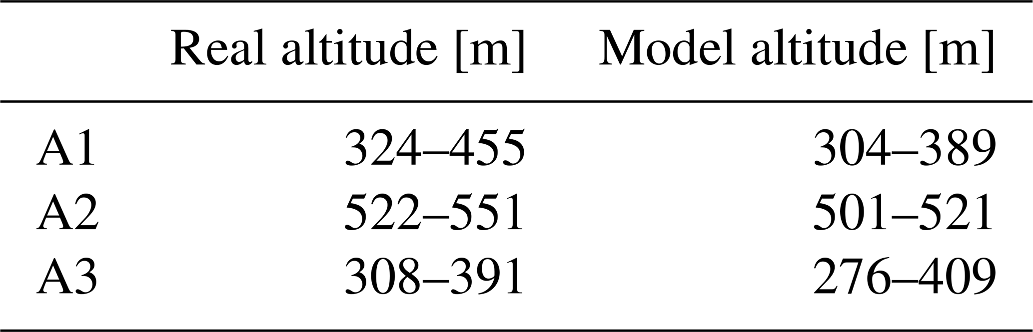
where θ is the potential temperature. It is assumed that the mountain will have an impact on the stable layer closest to the mountain top, and this layer is taken to have a depth of about 1 km, based on the typical stable layer in the selected cases. Δθ and Δz are therefore calculated between the lowest ERA5 model level (about 310 m a.s.l.) and model level number 120 (varying between 930–1000 m a.s.l.), noting that the ECMWF model levels are numbered from the model top downward. The potential temperature θ in Eq. (3) and the tangential wind speed U in Eq. (2) are calculated using model level number 127. With heights varying between 553–586 m a.s.l., the model level number 127 is the level closest to the real height of the mountain of wind park A. The mountain height h₀ is set to 550 m, according to the real terrain within the A2 turbine cluster (Table 1).

Additional non-dimensional parameters describing mountain wave characteristics are the vertical aspect ratio $h_{\mathrm{0}}/L$ and the hydrostaticity parameter $NL/U$, where L is the half width of the mountain. These are metrics describing whether the wave developing will be within the hydrostatic or non-hydrostatic regime. Mountain waves only exist when $NL/U>\mathrm{1}$. For $NL/U\gg \mathrm{1}$, vertically propagating waves dominate with minimal wave motion downwind (Jackson et al., 2013).

2.3 Model and simulation design

For the purpose of this study, the WRF model version 4.3 (Skamarock et al., 2019) is configured to include three two-way nested domains, D01, D02, and D03, with horizontal resolutions of 10.5 km, 3.5 km, and 700 m, respectively. The locations of the domains can be seen in Fig. 3. D01 and D02 consist of 101×101 and 112×112 grid points, respectively. D03 consists of 121 grid points in the north–south direction and 146 grid points in the east–west direction. Static fields with 30 arcsec resolutions are applied. The static fields are retrieved from the NCAR database and provided by the 20-category Moderate Resolution Imaging Spectroradiometer (MODIS) and the Global Multi-resolution Terrain Elevation Data 2010 (GMTED 2010). Table 1 summarises the real range of elevations within each turbine cluster of wind park A, along with the corresponding model elevations in D03. The vertical structure of the model consists of 51 terrain-following sigma levels, with the lowest five levels located below 100 m a.g.l. and the upper boundary at 50 hPa. The model is configured without Rayleigh damping.

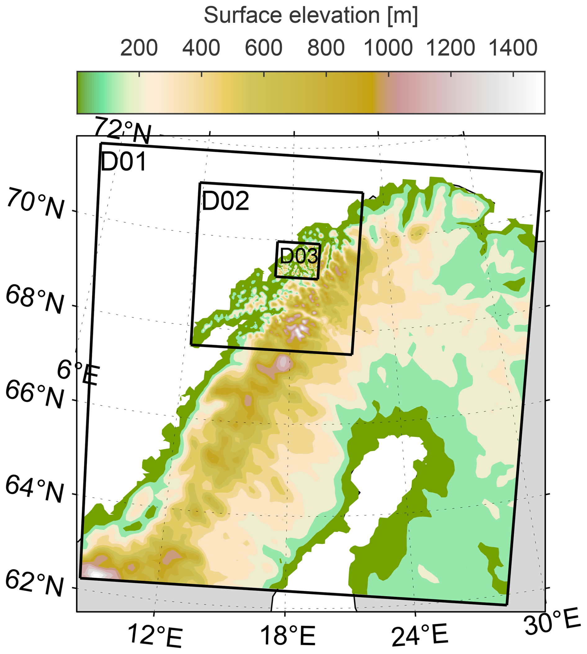
Figure 3 The WRF domain configuration, D01, D02, and D03, with terrain elevations within each domain, ranging from sea level (green) to 1500 m a.s.l. (white). The ocean surrounding the land area is also white.

The physical configuration of the model consists of the Thompson microphysics scheme (Thompson et al., 2008), the Rapid Radiative Transfer Model for Global applications (RRTMG) scheme for long- and shortwave radiation (Iacono et al., 2008), the MYJ surface layer scheme (Janjić, 1994), the Unified Noah Land Surface Model (Chen et al., 1997), the Mellor–Yamada–Nakanishi–Niino (MYNN) planetary boundary layer scheme (Nakanishi and Niino, 2009), and the Tiedke cumulus parameterisation scheme (Tiedtke, 1989; Zhang et al., 2011). For D03, the cumulus scheme was turned off due to the high resolution to allow the model to resolve the convective processes explicitly. Wind turbine parameterisation is applied by the Fitch scheme (Fitch et al., 2012). The power curve and thrust coefficient included are specific to the wind turbines in the park, with a default correction factor of 0.25, as suggested by Archer et al. (2020).

The ERA5 global reanalysis is used as initial and boundary conditions for the simulations. The simulations are run for 8 d, with the first 12 h considered spin-up time. The next 12 h of the simulation period has been interpolated with the last 12 h in the previous simulation to allow for smooth overlap of the time series. The simulations cover the period from 4 September 2020 to 24 January 2021. The wind data are retrieved 85 m a.g.l. by vertical interpolation of the model levels and from the given turbine locations by horizontal bilinear interpolation between the grid points. Similar to the observations, the cluster wind values and power production are the mean values of each parameter at the turbines within each cluster.

Table 1 The altitude variations at each turbine cluster based on 10 m resolution terrain data and model elevation data collected from domain D03. The values given in metres indicate the lowest and highest altitudes of the turbine locations within each cluster.

3 Results and discussion

For simplicity, this study only evaluates wind coming from the SE 120–165° sector. The observations from the A2 cluster indicate that the wind direction is within this SE sector for about 35 %–39 % of the study period. Furthermore, time slots, referred to as SE events, have been selected as described in Sect. 2.1. Within the study period, 67 SE events were selected, and, combined, these consist of 1104 h of data, corresponding to 32 % of the total study period. In the remainder of this study, all results presented and discussed are only related to the SE events.

3.1 Non-dimensional mountain height

This section investigates the relationship between the upstream weather conditions at location P (Fig. 1), calculated from ERA5 data, and the accelerated downslope winds in wind park A. The Scorer parameter and how this parameter changes with height indicate which type of mountain wave will develop during a mountain wave event. A cross-mountain wind decreasing with height, i.e. a reversed wind shear, is a condition where the Scorer parameter increases with height (Eq. 1). In addition, if the cross-mountain flow becomes zero and further reversed, the Scorer parameter goes to infinity with increasing height. Figure 4 illustrates the vertical profile of the tangential ERA5 wind speed at point P averaged over all SE events, with the tangential wind speed being the component of the horizontal wind in the SE direction. It is apparent that there is on average, for all 67 SE events, a reversed wind shear from about 900 m a.s.l. in the cross-mountain flow and a mean state critical layer at just below 8000 m a.s.l. This distinct signature in the upstream large-scale wind profile is quite striking and indicates upstream weather conditions in which mountain waves may either grow sufficiently to break and form a so-called “self-induced” critical level or propagate vertically, until they break at the mean state critical level. It is expected that the vertical wind profile will vary between the different events.

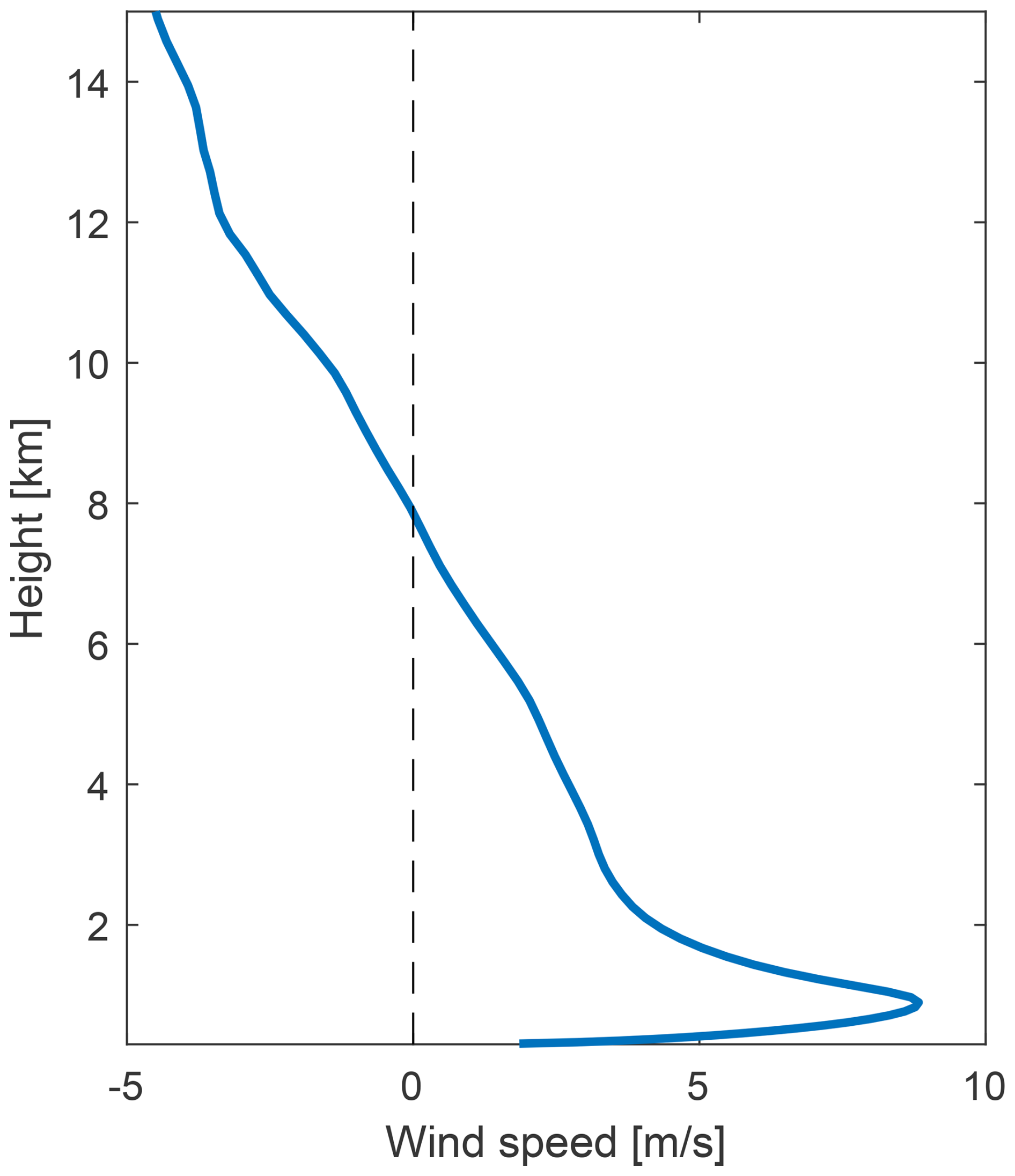
Figure 4 The vertical profile of the tangential ERA5 wind speed at location P averaged over all SE events, with wind speeds along the x axis and the average altitude above sea level along the right y axis.

Figure 5 illustrates the relationship between the downslope winds at A3 and the non-dimensional mountain height $\widehat{H}$. The y axis shows the A3 wind speed values normalised with respect to the wind speed at A2. The cluster wind speeds are the mean value of the observed nacelle wind speeds at the three turbines within each cluster, as defined in Sect. 2.1. A normalised wind speed above 1 means the wind speed is higher at the lee side than at the mountain top. The x axis shows the values of $\widehat{H}$ calculated from ERA5 data extracted at the upstream location P. The green dots show the hourly values, while the thicker blue dots represent the same values averaged over the period of each SE event. During the SE events studied, the wind speeds at the lee side of the mountain are typically stronger than the wind speed at the mountain top. When considering the hourly values of all SE events, the wind speed at A3 is higher than at A2 80 % of the time. In addition, 18 % of the time, the wind speeds are 1.5 times higher or more at A3 compared to A2. The non-dimensional mountain height varies mainly between 0 and 5 during the SE events considered. In addition, there are 10 sporadic timestamps (green dots) with $\widehat{H}$ values above 5 that are not included in the figure. As $\widehat{H}$ increases from zero to a value of about 1.5, there is a tendency of an increasing normalised wind speed. When $\widehat{H}$ increases further, the normalised wind speeds decrease. As $\widehat{H}$ increases above 3, the normalised wind speeds are typically below 1. These results correspond well with previous studies, such as Smith (1989) and Gaberšek and Durran (2004). Gaberšek and Durran (2004) studied idealised airflow over a mountain barrier and found that for $\widehat{H}$ lower than 0.25, mountain waves are created over the barrier, but no wave breaking is present, resulting in only slight enhancement of the wind speed downstream of the barrier. When the wind speed is increased such that $\widehat{H}$ equals 1.4, the wave breaks over the ridge and the wind speed increases in a narrow zone downstream of the barrier. In Gaberšek and Durran (2004), there is partial upstream blocking for $\widehat{H}=\mathrm{2.8}$ and full upstream blocking for $\widehat{H}=\mathrm{5.0}$. The current study shows a similar pattern with lower wind speeds at A3 than at A2 for $\widehat{H}$ above 3 according to Fig. 5, indicating upstream blocking and less air over the mountain. Sachsperger et al. (2016) found similar $\widehat{H}$ values for wave breaking in idealised flow over an obstacle. However, at what $\widehat{H}$ value the wave breaking first occurred also depended on the vertical aspect ratio. For aspect ratios of 0.1 and 0.05, wave breaking occurred when $\widehat{H}=\mathrm{1}$. For vertical aspect ratios outside of this range, wave breaking did not occur before $\widehat{H}=\mathrm{1.25}$ (Sachsperger et al., 2016). Along the SE direction, the mountain of wind park A is approximately 12 km wide at sea level, corresponding to a half width of 6 km and a vertical aspect ratio of about 0.09. The hydrostaticity parameter, given by $NL/U$, is estimated to be above 4 for all SE events and hence within the hydrostatic regime where waves propagate nearly hydrostatically.

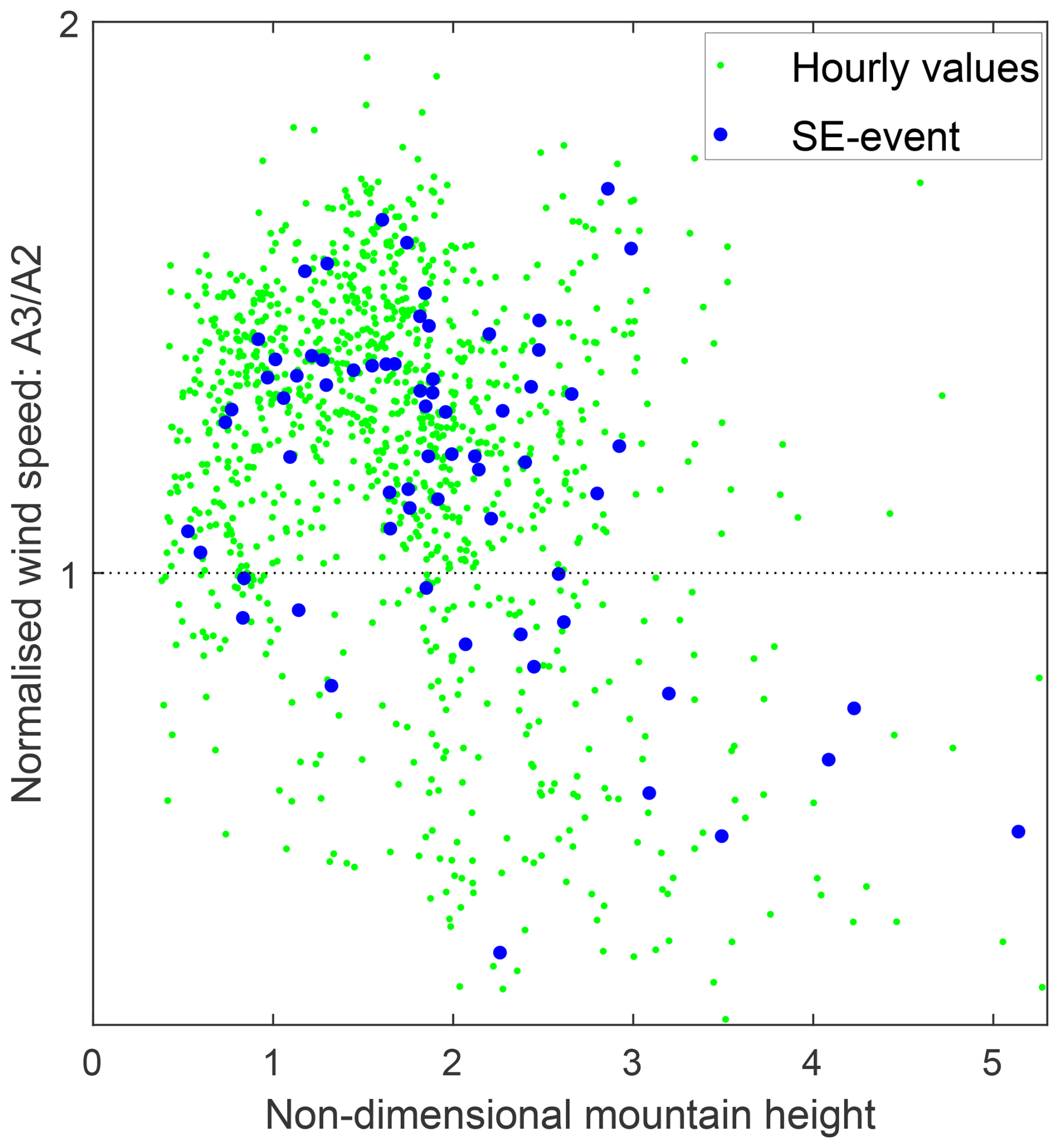
Figure 5 Scatter plots showing the hourly values (green dots) of the non-dimensional mountain height (x axis) and the A3 wind speeds (y axis) normalised with respect to A2 wind speeds. The blue dots indicate the average values taken over each SE event.

Figure 5 displays a strong relationship between $\widehat{H}$ and the A3 wind speeds, and for this particular wind park, the non-dimensional mountain height is to some extent able to indicate when to expect enhanced lee side winds due to mountain waves and when to expect lower wind speeds on the lee side of the mountain. The single parameter calculated from readily available meteorological data can hence be useful both in planning and for power prediction purposes. One reason the results appear to agree reasonably well with the theory may be that the lower-resolution ERA5 data, as opposed to local observations or high-resolution WRF simulations, provide a mean state of the atmosphere free of local terrain effects at location P. The apparent relationship between $\widehat{H}$ and the A3 wind speeds suggests that breaking of internal gravity waves is the dominant mechanism responsible for the strong downslope winds in wind park A.

Although the result of this study indicates a relationship between $\widehat{H}$ and the downslope winds at A3, the results should be interpreted with caution. In particular, the approximation of a constant Brunt–Väisälä frequency is not straightforward, as demonstrated by Reinecke and Durran (2008). Reinecke and Durran (2008) applied two common approximations for N, referred to as the averaging method and the bulk method, to multiple cases with vertically nonuniform stability. Neither of the two methods provided a single best method to estimate a constant N. However, compared to the averaging method, the bulk method provided a better prediction of whether a flow will pass over the mountain or around it. To account for the uncertainty in estimating N and U, sensitivity analyses are performed. As described in Sect. 2.2, N is estimated using the bulk method in Eq. (2) between the ERA5 model levels spanning the surface up to a height of about 1 km. The sensitivity in the approximation of N is tested by changing the upper level to heights of about 855 and 1172 m a.s.l. The results (not shown) appear to be only weakly sensitive to the choice of the upper vertical level used to calculate N, with the overall findings remaining consistent. U in Eq. (2) is approximated from the single ERA5 level closest to the mountain peak (about 580 m a.s.l.). The sensitivity to the approximation is evaluated by calculating U at heights slightly below (500 m a.s.l.) and above (677 m a.s.l.) mountain top level. The results (not shown) are only weakly sensitive to the choice of the model level.

The sensitivity to upstream geography is tested by dividing the SE wind sector into two smaller sectors. In the first sector (120–140°), the nearby upstream terrain is characterised by several high mountains (Fig. 1). In the second sector (140–165°), the airflow approaches the wind parks rather undisturbed through a long fjord. The distinction between the two sectors is made based on observed wind directions from one of the A2 turbines. Figure 6a shows the results for the first sector and Fig. 6b for the second sector. Within the first sector, there is a tendency of increasing normalised wind speeds as $\widehat{H}$ increases towards 1; however, similar to Fig. 5, there are some deviating wind speed values for $\widehat{H}\sim$ 1. Within the second wind sector, the relationship between $\widehat{H}$ and the normalised A3 wind speed appears to agree better with the theory, with less spread in the normalised wind speeds when $\widehat{H}\sim$ 1 and no normalised wind speed values below unity for $\widehat{H}<\mathrm{1.6}$. Figure 6b supports our view that one of the reasons why the rather simple theory of the non-dimensional mountain height appears to hold to some extent in this real-world case, as opposed to an idealised model, may be the long and well-defined fjord that channels the wind from location P towards the mountain.

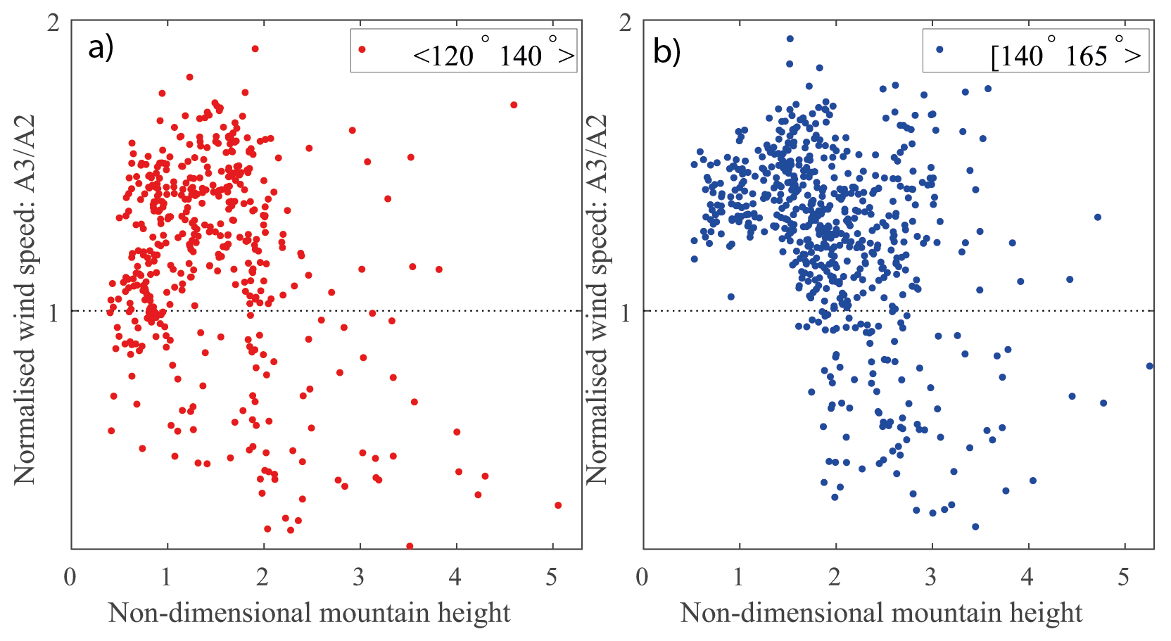
Figure 6 Similar to Fig. 5. (a) Hourly values for the 120–140° sector. (b) Hourly values for the 140–165° sector.

Although many of the events appear to be consistent with the theory, there are also several events that deviate. This is not unexpected, as the concept of the non-dimensional mountain height is developed based on linear flow with approximately uniform U and N. However, the apparent relationship between the non-dimensional mountain height and the A3 wind speeds is encouraging. Future work should address additional metrics, such as the Froude number, developed based on hydraulic theory. In addition, future research should test whether a similar relationship exists in other wind parks located in comparable terrain.

3.2 Downslope winds and impact on power production

The impact of mountain waves and strong downslope winds on wind power production is evaluated in terms of the wind speed distribution and the power production at the three wind turbine clusters. These results include only wind and power production for the SE events selected as described in Sect. 2.1. Figure 7a shows the variations in the observed wind speed distribution between clusters A1 (blue), A2 (green), and A3 (red) when only the SE events are included. The histogram bins have been divided into intervals of 0.5 m s⁻¹ along the x axis, and the frequency on the left y axis is given in 10 min values that have been converted to hours. In order to allow for a comparison of the wind speeds and the potential power production, the power curve for the turbines has been included in the same figure (black dashed line) with power along the right y axis. The power curve consists of four power curve zones (PCZs): PCZ1, with wind speeds below the cut-in threshold and no power production; PCZ2, with wind speeds between the cut-in wind speed and the rated wind speed, i.e. where the power increases from zero and up to the rated power; PCZ3, where the turbines operate at rated power until cut-off wind speed; and PCZ4, the zone where the turbines are shut down due to high wind speeds. For the turbines in these particular wind parks, the cut-in wind speed is at 3.0 m s⁻¹, the cut-off wind speed is at 28.5 m s⁻¹, and the rated wind speed is 14.5 m s⁻¹.

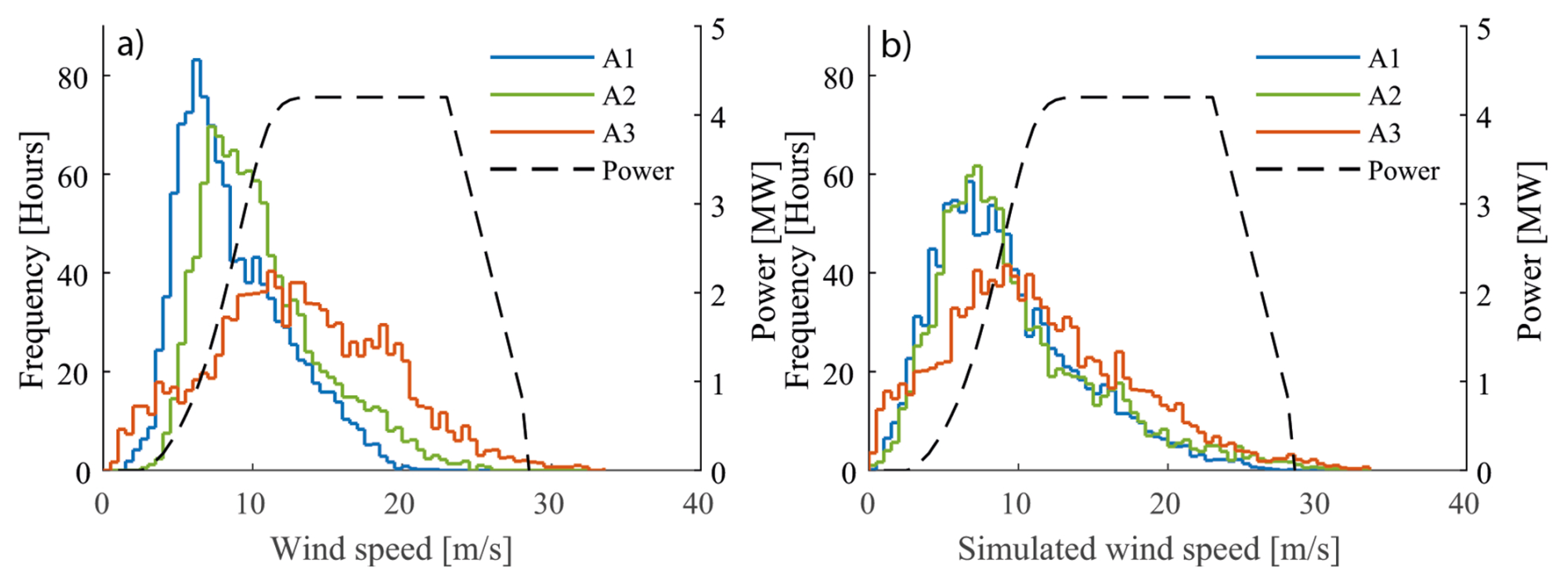
Figure 7 (a) Observed wind speed frequency distributions for the turbine clusters at A1 (blue), A2 (green), and A3 (red), with wind speeds along the x axis and wind speed frequency in hours along the left y axis. The dashed line represents the turbine power curve, and the values are indicated along the right y axis. (b) Similar to (a) but representing the simulated wind speeds.

The A3 wind cluster has a higher frequency of wind speeds favourable for wind power production in comparison to A1 and A2. While the A1 and A2 wind speed distributions have similar shapes, shifted towards the left, with peaks at approximately 6 and 7 m s⁻¹, respectively, the A3 wind speeds are more evenly distributed, with a peak around 11 m s⁻¹. At A1 and A2, the frequency of wind speeds within PCZ2 is considerably higher than at A3. Consequently, the A1 and A2 turbines operate below the rated power more often compared to A3. In addition, small variations in wind speed within PCZ2 result in large variations in power production. At A3, on the other hand, the frequency of wind speeds within PCZ3 is considerably higher than at A1 and A2; hence the A3 turbines will more often operate at their maximum power. In addition to the enhanced power production on the lee side of the mountain of wind park A, the same wind turbines record wind speeds above the cut-off threshold and below the cut-in threshold more often than the turbine clusters upstream. The large difference in the wind speed distribution between A3 and the two other clusters has a clear impact on wind power production and is expressed through the capacity factor C_f in Table 2. The capacity factor is a parameter commonly used to evaluate how well sited a wind turbine is and is defined as the ratio of the actual energy produced to its maximum possible energy output over the same period. For the purpose of this study, C_f is calculated from the power produced during the SE events only. The A3 turbines operate considerably closer to their maximum in comparison to the turbines in the other two clusters. During the selected SE events, the A3 turbines produce 51 % and 21 % more energy than the A1 turbine and A2 turbines, respectively.

Similarly, the wind speed distributions (not shown) for the three clusters in wind park B, as indicated in Fig. 2, reveal a higher frequency of higher wind speeds on the lee side compared to the upstream turbines, although the difference between the clusters is not as pronounced as in wind park A. The capacity factor in Table 2 reflects the spatial variations within wind park B, with C_f being the highest at B3 and the lowest at B1.

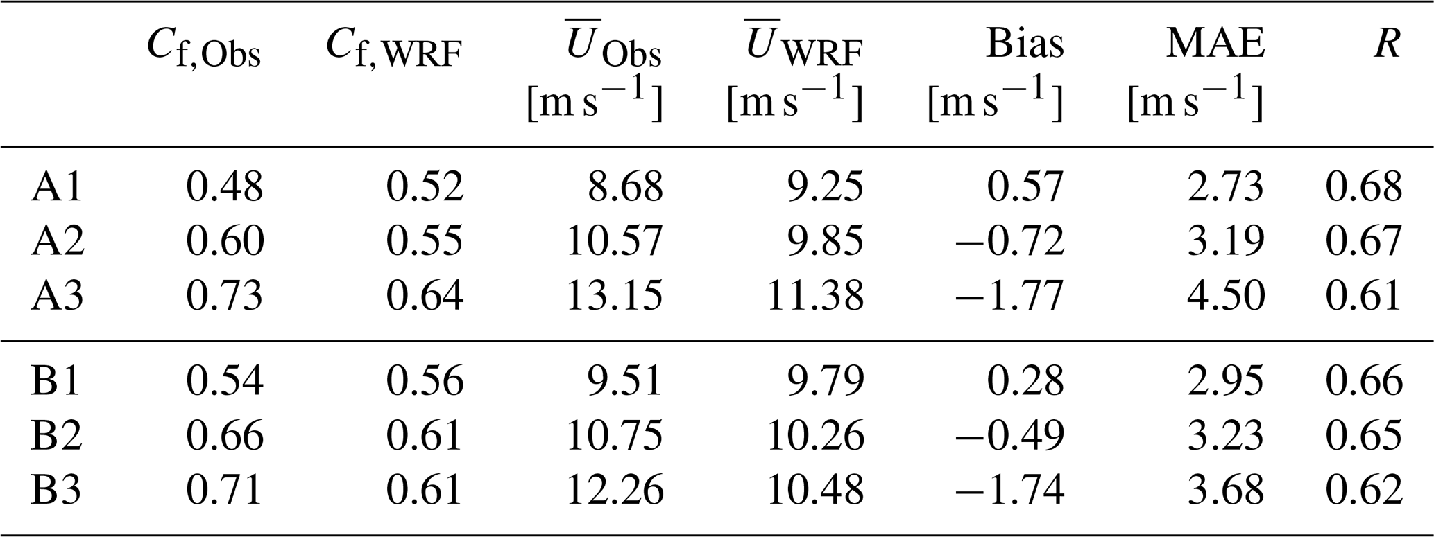
Table 2 The observed and simulated capacity factor C_f and mean wind speed $\stackrel{\mathrm{‾}}{U}$, as well as the bias, the MAE, and the correlation coefficient R between the observed and simulated wind speeds.

The result of this study emphasises the importance of an extensive understanding of the wind flow in complex terrain during various atmospheric stability conditions, both in the planning phase and for wind power production forecasts. Although there were no observations of severe wind speeds in these particular wind parks during the study period, downslope windstorms can result in severe and occasionally damaging wind speeds, large wind speed fluctuations, and turbulence and wind gusts (Klemp and Lilly, 1975; Durran, 1990) and should therefore be considered in the planning phase.

3.3 WRF

The ability of the WRF model to reproduce the observed wind patterns in the wind parks is evaluated in terms of the mean features during the SE events, such as the wind speed distribution, the mean wind speed, and the capacity factor calculated over the same periods. In addition, the ability of the model to reproduce the temporal pattern of the observations is evaluated in terms of the mean absolute error (MAE) and the correlation coefficient (R). These statistical parameters and the bias are also provided in Table 2 and are calculated as described in Solbakken et al. (2021). In addition, the ability of the WRF model to reproduce the wind directions during the SE events is evaluated in terms of wind roses (not shown) for all nine turbines within the clusters in wind park A. WRF is able to reproduce the wind directions with only small deviations from the observations.

In agreement with the observations, the simulations show a higher mean wind speed at the lee side of the mountain (A3) compared to the mean wind speeds at the mountain top (A2) and at the upstream location (A1). When evaluating each turbine cluster separately, the wind speed bias indicates that the model tends to overestimate the wind speeds at A1, while underestimating the wind speeds at A2 and A3. The negative bias at A3 is considerably larger than at A2. The larger negative bias at A3 suggests that the model is not fully able to reproduce the accelerated downslope winds. The WRF model is also able to reproduce the spatial variations in power production, with the highest C_f at A3 and the lowest C_f at A1. Although the model is, to some extent, able to reproduce the relative power production of the three turbine clusters, the increase in C_f from A1 to A2 and A3 is not as pronounced as what is seen in the real C_f. Similar wind speed biases are found in the clusters of wind park B. Although the model is able to reproduce the higher mean wind speed at B3, compared to B2, WRF is not able to reproduce the increase in C_f from the B2 cluster to the B3 cluster.

When comparing the temporal patterns of the simulations and observations, the MAE is the lowest at A1, higher at A2, and the highest at A3. The correlation coefficient is the highest at A1 and the lowest at the A3 cluster. Wind park B exhibits similar patterns in MAE and R (Table 2), with higher error and lower correlation at B3 compared to the turbine clusters upstream. The reduced accuracy in the temporal pattern at the lee side turbines is also seen in the study by Rögnvaldsson et al. (2011) and can be linked to the increased complexity of the wind patterns from the windward side to the lee side due to mountain waves. The MAE and the R of the current study are of similar values as in previous studies conducted in the same area (Solbakken et al., 2021; Solbakken and Birkelund, 2018). In addition, the MAE and the R in the current study, with a 700 m horizontal grid resolution, are slightly improved compared to what was found in the 1 km simulations by Solbakken et al. (2021) at the same location. However, the results are not directly comparable due to differences in the model configurations and study periods.

Figure 7b presents the wind speed distributions of the simulated wind speeds at the three turbine clusters in wind park A. The WRF model is able to reproduce the observed differences between the A3 wind speed distribution and the distributions of the other two clusters. In agreement with the observations, there is a high occurrence of wind speeds above 12 m s⁻¹ at A3, including wind speeds above the cut-off threshold, while at A1 and A2 there is a lower occurrence of the same wind speeds. The higher occurrence of the PCZ3 and PCZ4 wind speeds at A3 compared to A1 and A2 indicates that the model is able to simulate the formation of mountain waves above the wind park causing the accelerated winds on the lee side of the mountain. For the lower wind speeds, below the cut-in threshold, the model succeeds in reproducing the higher occurrence of these wind speeds at A3 compared to A1 and A2. This result suggests that the model is also able to reproduce periods where the airflow is blocked by the mountain and diverted around.

Although the model is able to reproduce the distinct wind speed distributions observed at the three clusters, the distributions also reveal some shortcomings in the ability of the model to accurately reproduce the complex wind patterns in the wind park. For instance, the differences between the simulated wind speed distributions of the three clusters are not as pronounced as they are in the observations. In particular, the A1 and A2 wind speed distributions appear to be more similar in comparison to the observed wind speed distributions at the same locations. When comparing the simulations with the observations at the A3 cluster, it is apparent that the model underestimates the high occurrence of the PCZ3 wind speeds. The underestimations of these higher wind speeds suggests that the model is not fully able to reproduce the frequency and the strength of the downslope windstorms. It is worth noting that for the highest wind speeds at A3, above the cut-off threshold, the simulated wind speeds are more accurate. At A2 the simulated wind speed distribution skews left in comparison to the one of the observations. In particular, the model overestimates the frequency of the lower wind speeds and underestimates the higher wind speeds. At A1, the model considerably underestimates the lower PCZ2 wind speeds, while overestimating the occurrence of the wind speeds within the PCZ3. The shift in the simulated wind speed distribution, with under- and overestimation in PCZ2 and PCZ3, respectively, agrees well with previous studies conducted in the same area (Solbakken and Birkelund, 2018; Solbakken et al., 2021). However, for the lower wind speeds, below the cut-in threshold, the model overestimates the frequency at all three turbine clusters. A similar overestimation of the lower wind speeds is not seen in the studies of Solbakken and Birkelund (2018) and Solbakken et al. (2021).

Several factors may impact the accuracy of the model simulations. For instance, Reinecke and Durran (2009) found that small variations in the initial conditions led to substantial differences between forecast ensembles of downslope windstorms, including qualitative differences in the characteristics of the upper-level wave breaking, as well as in the strength of the downslope winds, while Rögnvaldsson et al. (2011) highlighted the importance of micro-physical processes in the formation of downslope windstorms. The accuracy of numerical simulations of downslope winds is also highly sensitive to the accuracy of the roughness length, land use, and surface friction parameterisation (Shestakova, 2021; Reinecke and Durran, 2009; Sachsperger et al., 2016).

A higher horizontal resolution, hence, a better representation of mountain peaks in particular, is also expected to improve the accuracy of simulated meteorological metrics during mountain wave events (Samuelsen and Kvist, 2024; Wagner et al., 2017). Although the mountain peaks appear to be sufficiently represented in the model (Table 1), a higher resolution could improve the representation of the terrain, as well as some smaller-scale terrain features that are missing in the model and may impact the accuracy of the simulations. In addition, the terrain model used to configure WRF has a resolution of 30 arcsec and is part of the default setup of the WRF model. However, higher-resolution terrain models are available and could potentially improve the terrain representation in D03.

For the purpose of the current study, the horizontal resolution is carefully selected to balance the benefits of higher-resolution details with the constraints imposed by the Fitch wind farm parameterisation, which recommends a grid size of at least 5 rotor diameters (Fitch et al., 2012). For this particular study, given that the mountains of the wind park are approximately 10 km across, a 700 m grid resolution, corresponding to an effective resolution of $\mathrm{7}\times \mathrm{\Delta }x\approx$ 4.9 km, may not adequately resolve the mountain-induced flow perturbations. Perturbations, such as mountain waves, on scales smaller than the effective resolution are damped and likely contribute to the model not being able to reproduce some of the observed variability in the wind (Skamarock, 2004). Future studies should evaluate the potential benefits of a finer grid resolution, though this would require reconsideration of the turbine representation.

Another factor impacting the wind flow within the park is the wakes created by the wind turbines. Studies suggest that under stable conditions, the strength of the wakes is higher and the recovery slower than during unstable and neutral conditions (Han et al., 2018). For the purpose of the current study, the Fitch wind farm parameterisation scheme is employed in the model to allow for the impact from the wind turbines on the simulated wind flow. However, the accuracy of wind power parameterisation schemes under stable atmospheric conditions is not thoroughly explored. For instance, García-Santiago et al. (2024) found that when comparing mesoscale simulations with large-eddy simulations, the Fitch scheme exhibits larger deviations under stable atmospheric conditions than during neutral or unstable atmospheric conditions. In addition, the Fitch scheme does not take into account mechanical and electrical losses, resulting in an overestimation of the turbulent kinetic energy (TKE) generated by the turbines in the model (Fitch et al., 2012). In order to reduce the TKE source, Archer et al. (2020) suggest the introduction of a correction factor. Due to the lack of a reliable estimate for the correction factor during stable atmospheric conditions, the initially suggested correction factor of 0.25 (Archer et al., 2020) is employed in the simulations of the current study. However, the study by García-Santiago et al. (2024) suggests that under stable conditions, as compared to neutral conditions, an increased correction factor could improve the simulation results.

This study demonstrates the ability of the WRF model to reproduce spatial patterns of hub height wind speeds relevant for wind power production in complex terrain. It is possible that tuning the model configuration to more optimal settings could further improve the simulation results, particularly if the stability is affected (Rögnvaldsson et al., 2011). A future study should therefore include a sensitivity analysis and investigate the impact of the wind farm parameterisation on the wind field within the parks during periods with strong downslope winds.

3.4 Case studies

The following analysis investigates two different events. Case 1 represents a typical SE event, with stronger winds at A3 compared to A2. Case 2 represents a less frequent event, with weaker wind at A3 compared to A2. The analysis is motivated by the observations showing that under comparable wind directions, the wind speeds and power production at A3 relative to A2 can vary substantially.

3.4.1 Case study 1: mountain-wave-induced accelerated wind speeds

The first case study is the SE event running from 24 December 2020 at 23:20 local time (LT) to 25 December 2020 at 23:20 LT, where a strong downslope wind is observed. Figure 8a shows the Scorer parameter at every hour during the period considered. At 05:00 LT, the Scorer parameter is nearly constant between 1000 and 1500 m a.s.l. and increases between 1500 and 2500 m a.s.l., indicating conditions where vertically propagating mountain waves may form and break. A critical layer is present at heights from about 4500 m a.s.l. Figure 8b shows that the non-dimensional mountain height decreases from 2.8 to 1 during the period of the case study. Based on the results in Sect. 3.1, these are $\widehat{H}$ values where strong downslope winds are expected at the A3 cluster.

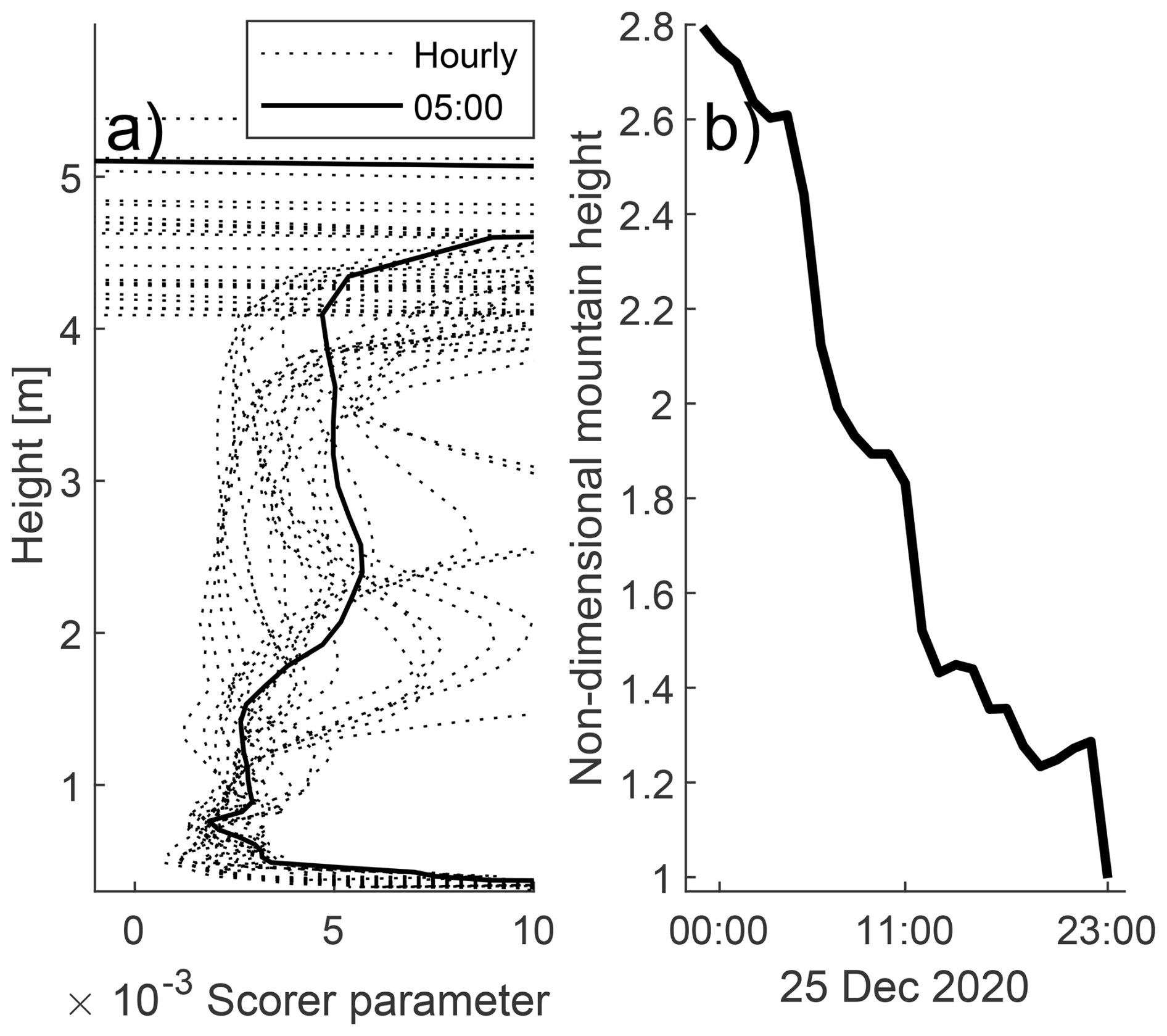
Figure 8 Case study 1 on 25 December 2020. (a) Hourly Scorer parameter (dotted) and at 05:00 LT (solid) (along the x axis) at altitudes indicated along the y axis. (b) The non-dimensional mountain height $\widehat{H}$.

Figure 9 presents the observed (left) and simulated (right) wind speed (top), wind directions (middle), and power production (bottom) during this event for the turbine clusters A1 (blue), A2 (green), and A3 (red). The observed wind directions at the three turbine clusters vary between 140–165°. The observed wind speeds at A3 vary between 11 and 19 m s⁻¹ and are persistently stronger than the wind speeds at A1 and A2, where the wind speeds vary between 5 and 13 m s⁻¹. Consequently, the A3 turbines operate at rated power nearly throughout the entire 24 h period, while the A1 and A2 clusters encounter a considerably lower power production, particularly during the first 12 h. The simulated wind directions exhibit larger variations within a slightly larger sector compared to the observations. In agreement with the observations, the simulated wind speed is higher at A3 than at A1 and A2. However, compared to the rather steady observed wind speeds, the simulated wind speeds exhibit large temporal variations. The simulated power production is higher at A3 compared to A2 and A1, although with large oscillations at all clusters due to the erroneous variations in the simulated wind speeds.

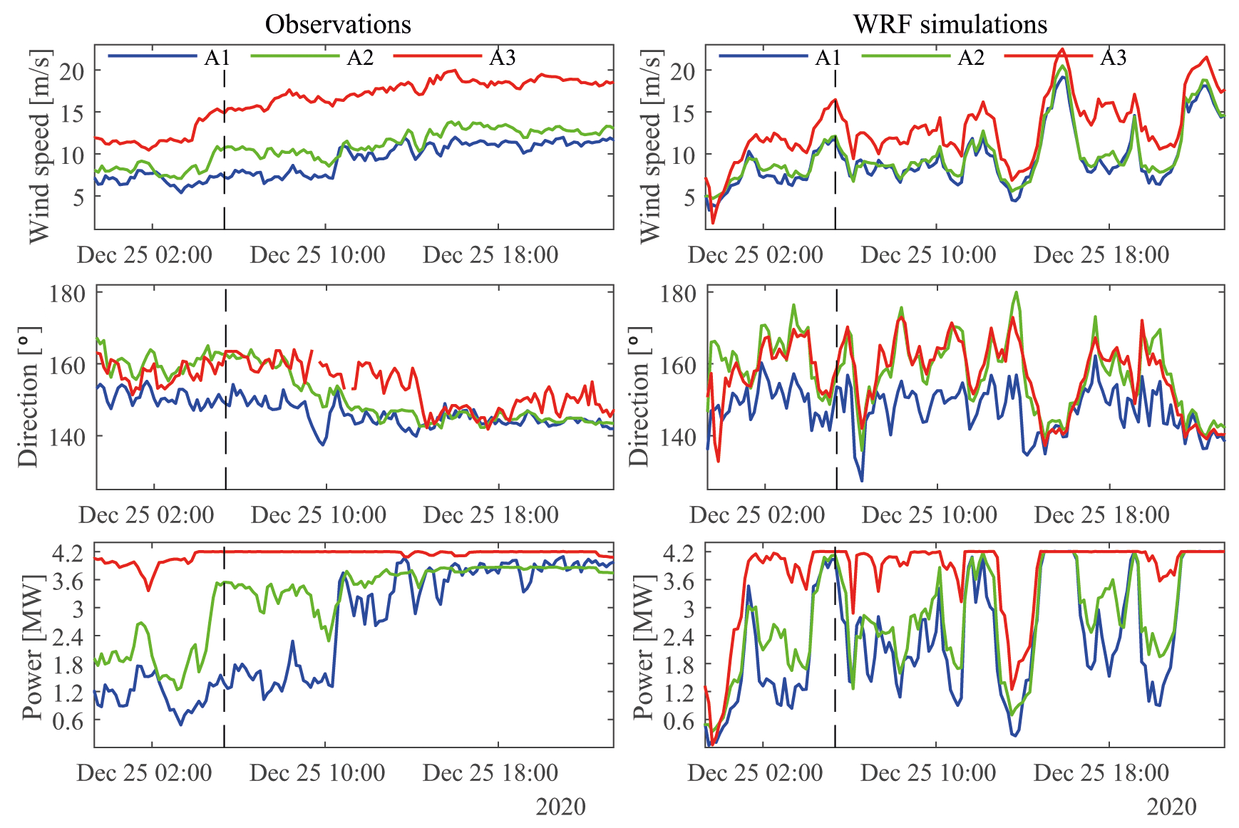
Figure 9 Observed (left) and simulated (right) wind speeds (top), wind directions (middle), and power production (bottom) for the three wind turbine clusters A1 (blue), A2 (green), and A3 (red) on 25 December 2020. The vertical dashed lines indicate the time of Fig. 10.

Figure 10 presents the observed and simulated winds on 25 December 2020 at 05:20 LT, indicated with the dashed line in Fig. 9. Figure 10a shows the observed wind speeds and Fig. 10b the simulated wind speeds at hub height (85 m a.g.l.) at each wind turbine. The observed wind speeds range from 5 (blue) to 15 m s⁻¹ (orange). The turbines upstream of the mountain top exhibit wind speeds ranging from about 5 to 10 m s⁻¹, while the turbines on the mountain top encounter slightly higher wind speeds. The highest wind speeds of 15 m s⁻¹ are found on the lee side of the mountain, particularly within turbine cluster A3. In general, the WRF simulations reproduce the spatial wind pattern that is apparent in the observations well. However, the simulated wind speeds in the wind parks are in general overestimated and have less spatial variations in wind speeds within the wind parks compared to the observations.

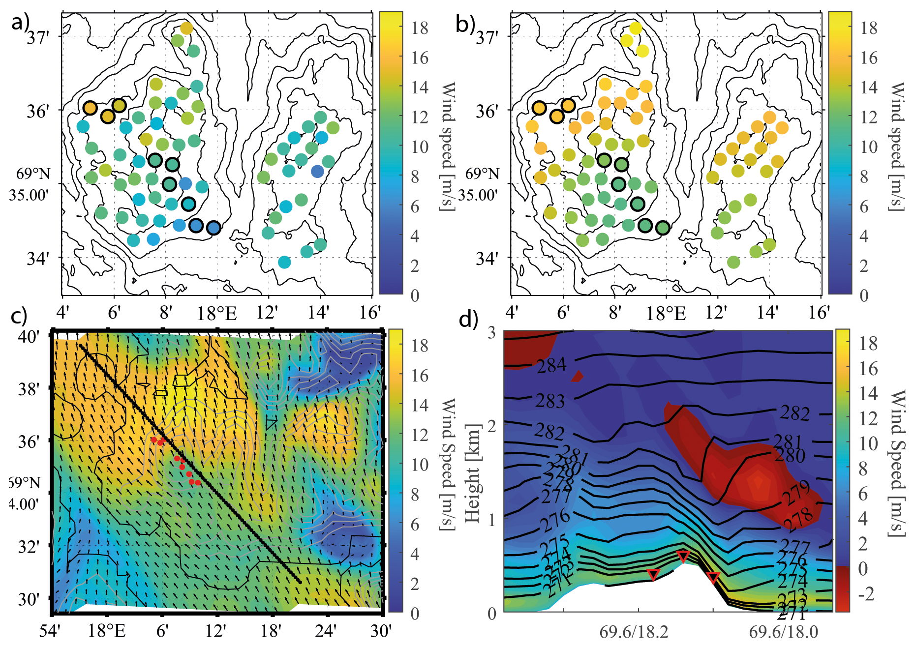
Figure 10 (a) Observed and (b) simulated horizontal wind speeds at 85 m a.g.l. at the turbine locations. Ü(c) Horizontal wind speed at 85 m a.g.l. The solid contours indicate the land areas, and the grey solid contours indicate the model terrain elevation with 100 m intervals. The red dots indicate the locations of the turbines within clusters A1, A2, and A3. The wind speeds range from 0 m s⁻¹ (dark blue) to 19 m s⁻¹ (yellow), and the arrows indicate the wind direction. (d) Vertical cross section in the SE–NW direction, as indicated by the solid black line in panel (c), showing the potential temperature (black lines) with a line spacing of 1 K. The colours blue (0 m s⁻¹) to yellow (19 m s⁻¹) indicate positive tangential wind speeds in the SE direction, while the red colours indicate reversed wind speeds, ranging from −3 to 0 m s⁻¹. The terrain is indicated in white, and the three turbine clusters are marked with triangles at their approximate location. All figures are from 25 December 2020 at 05:20 LT.

Figure 10c displays the spatial variations in the simulated horizontal wind speeds at 85 m a.g.l. over a slightly larger area than Fig. 10a and b. The airflow approaches the mountain from the southeast, with a relatively unidirectional flow across the mountain. The wind speeds on the windward side and over the mountain top are of a similar magnitude, while on the mountain lee side there is a large area of higher wind speeds, including the location of the A3 wind turbines.

The vertical cross section of the simulated tangential wind speeds and the potential temperature in Fig. 10d suggests mountain-wave-induced accelerated winds on the lee side of the mountain. The position of the vertical cross section is indicated by the southeast- to northwest-oriented solid line in Fig. 10c, and the tangential wind speed is the horizontal wind speed decomposed in the approximate direction of the cross section. The potential temperature increases with altitude, and a reversed wind speed shear is present from the surface level up to about 3000 m a.s.l., in which the wind speed becomes negative, indicating the presence of a critical layer. The mountain waves are apparent from the isentropes. The growing wave amplitude, the upstream-tilting isentropes, and the locally reversed winds suggest wave breaking with a self-induced critical layer at about 1000–2000 m a.s.l. above the mountain. This is in accordance with the Scorer parameter in point P. As shown in Fig. 8, the parameter indicates conditions that favour vertically propagating mountain waves and wave breaking between 1000–2500 m a.s.l. Beneath the stagnant area, the isentropes are compressed, and the wind speeds accelerate towards the surface on the lee side of the mountain with wind speeds exceeding 15 m s⁻¹ (orange).

3.4.2 Case study 2: partial blocking

The second case study is on 11 December 2020 at 08:20 to 19:20 LT, with weaker wind speeds on the lee side than upstream. In this case study, Fig. 11a depicts a Scorer parameter with large variations over time. At 12:00 LT (solid line), the Scorer parameter is near constant at the lowest levels and increases from about 1500 to 2500 m a.s.l., indicating upstream weather conditions favourable for the development of vertically propagating and breaking mountain waves, as well as the presence of a critical layer. However, the Scorer parameter is only relevant when the air flows over the mountain. In this case study, the non-dimensional mountain height, in Fig. 11b, varies between values above 3, where upstream blocking is expected to occur, and below 3, indicating accelerated downslope winds at A3 according to the results in Sect. 3.1. At 12:00 LT, $\widehat{H}$ is 2.6.

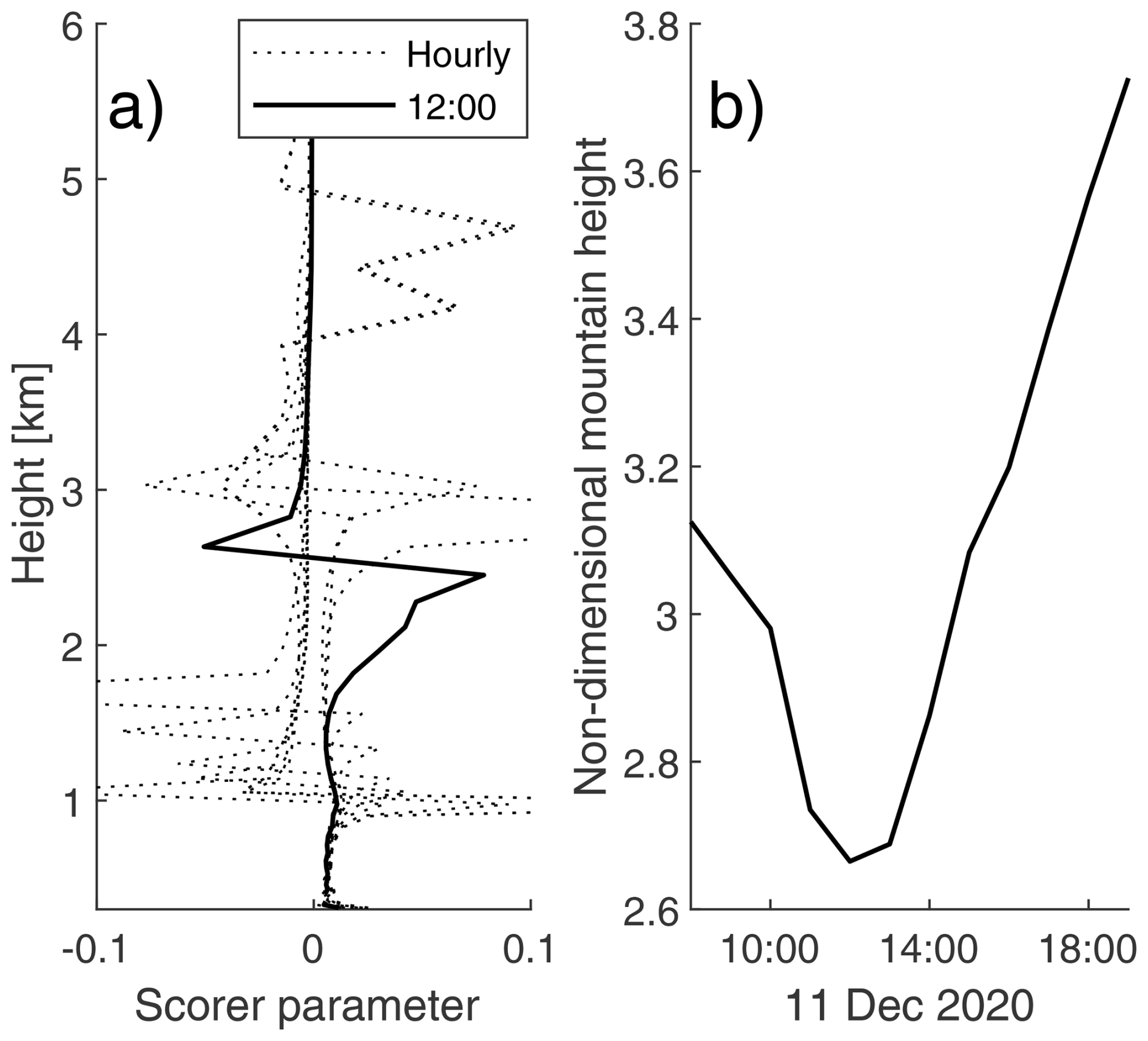
Figure 11 Case study 2 on 11 December 2020. (a) Hourly Scorer parameter (dotted) and at 12:00 LT (solid) (along the x axis) at altitudes indicated along the y axis. (b) The non-dimensional mountain height $\widehat{H}$.

Figure 12 shows wind speeds, wind directions, and power production in a similar manner as in Fig. 9. The wind directions at A1 and A3 vary mainly between 130 and 155° throughout the period considered. The wind at A2 has a slightly stronger southerly wind component. The wind is relatively weak at all clusters, with the A3 wind being generally weaker than the wind at A1 and A2. However, the A3 wind speeds occasionally exceed the wind speeds at the turbine clusters upstream. These wind speed peaks indicate that the kinetic energy may occasionally become sufficient to allow for flow over the mountain and mountain waves to form. This observation does to some extent agree with the variations in the non-dimensional mountain height in Fig. 11, although the temporal pattern does not align with the A3 wind speed peaks. In addition to the limitation of the theory of the non-dimensional mountain height discussed in Sect. 3.1, the absence of a clear correlation between $\widehat{H}$ and the A3 wind speed pattern may, for instance, be attributed to the different temporal resolutions of the two datasets, with the hourly ERA5 data not providing the same level of temporal details as the 10 min observational data from the wind park. Furthermore, the low wind speeds are reflected in the power production, with power production below 1 MW at all clusters. The power production is the lowest at A3, where the wind speeds are below the cut-in threshold on several occasions. WRF is able to reproduce the observed wind and power production well between 09:00 and 15:00 LT. The simulated wind directions vary between 130 and 170°, and in agreement with the observations, the wind has a slightly more southerly component at A2 than the wind at the other two clusters. The simulated wind speeds correspond well with the observations; however, the periods with weaker winds at A3 compared to the upstream clusters are shorter than in the observations, and the peaks, where the A3 wind speed exceeds the A1 and A2 wind speeds, last longer. After about 15:00 LT, agreement between the observations and the WRF simulations is reduced. The WRF simulations exhibit larger variations in the wind direction at A2 and A3 compared to the observations, and the wind weakens to below the cut-in threshold at all clusters.

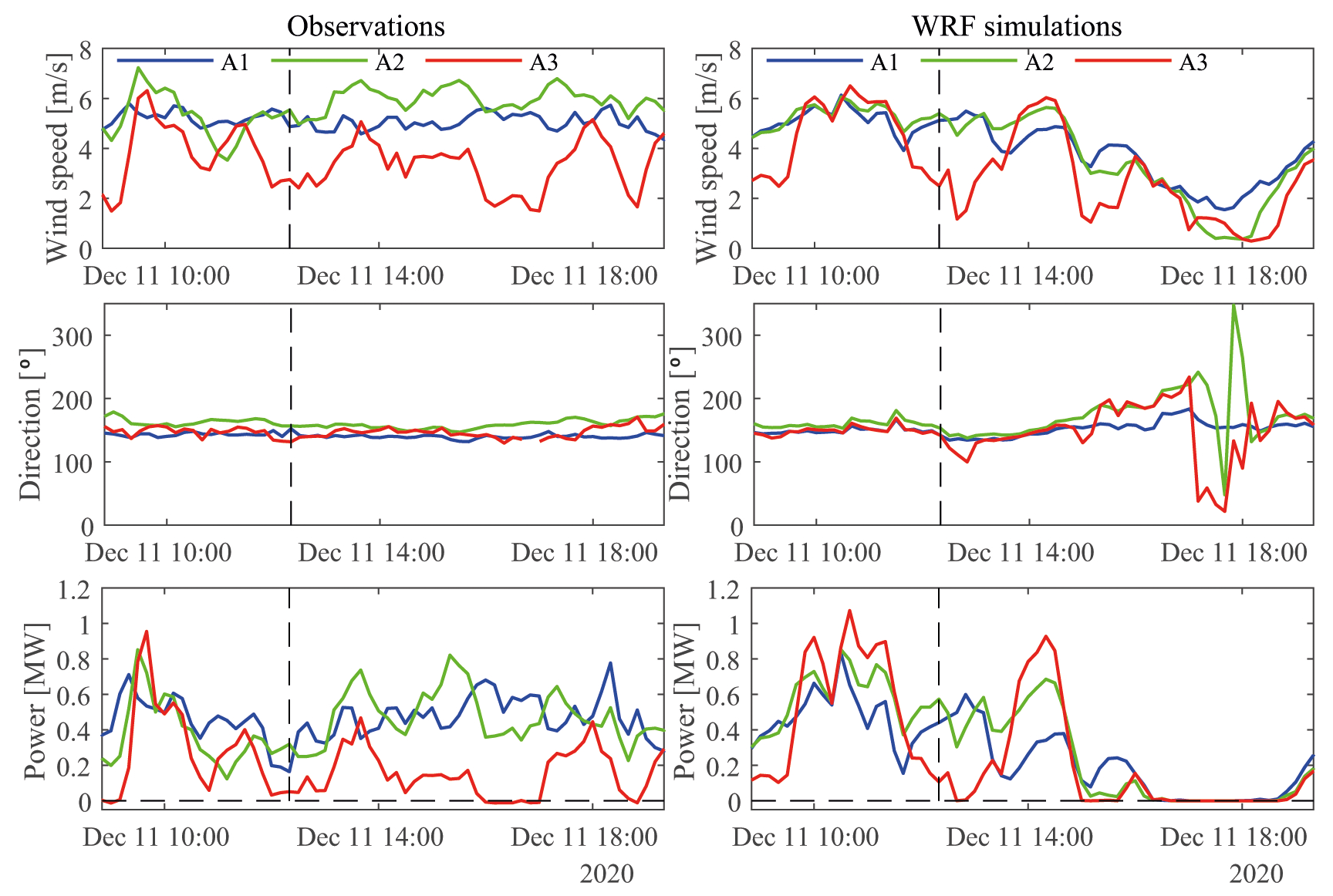
Figure 12 Observed (left) and simulated (right) wind speeds (top), wind directions (middle), and power production (bottom) for the three wind turbine clusters A1 (blue), A2 (green), and A3 (red) on 11 December 2020. The vertical dashed lines indicate the time of Fig. 13.

Figure 13 is similar to Fig. 10 but represents the second case study on 11 December at 12:20 LT. The observed wind speeds in Fig. 13a vary between 1 and 8 m s⁻¹. At wind park A, the winds are weak across the mountain top, and the lowest wind speeds, close to the cut-off threshold, are found on the mountain lee side. The turbines located on the mountain sides parallel with the airflow encounter the highest wind speeds. The WRF model is able to reproduce the spatial pattern of the observations well, with weak wind across the mountain top, considerably lower wind speeds on the mountain lee side, and the strongest winds on the western side of the wind park, as seen in Fig. 13b. The simulations have slightly less spatial variations in comparison to the observations, with simulated wind speeds ranging from about 2 to 7 m s⁻¹.

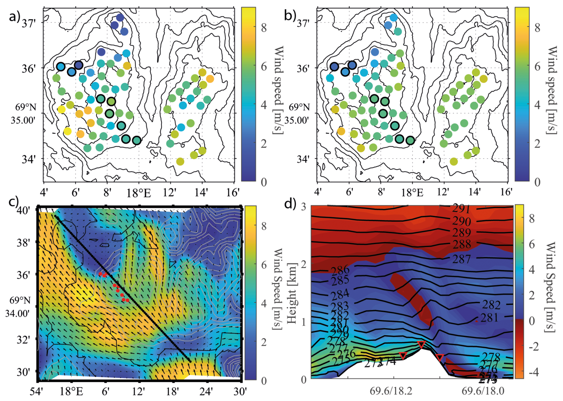
Figure 13 Similar to Fig. 10 for case study 2 on 11 December 2020 at 12:20 LT.

Figure 13c reveals large variations in horizontal wind speeds over the mountain areas, from 0 m s⁻¹ up to 9 m s⁻¹ on the western side of the mountain of wind park A. The wind approaches the mountain from the SE. Just below the mountain top, the wind decelerates, and the arrows indicate that some of the airflow is diverted around the mountain. On the lee side of the mountain, the horizontal wind speed drops to near-zero values over a large area. The weak winds in this area are interpreted to be a result of partial upstream blocking. Partial upstream blocking occurs when a stagnation point develops on the windward side of the mountain and is described in Baines and Smith (1993). Below this point, the wind is diverted horizontally around the mountain, resulting in a lee side wake with eddy formation. The air above the stagnation point will pass over the mountain; however, the efficient height of the mountain will be reduced. An alternative explanation is that the large blue area of weak winds results from atmospheric rotor formation downstream of a downslope windstorm (Mobbs et al., 2005). However, the absence of accelerated winds at the leeward turbines suggests otherwise.

The vertical cross section in Fig. 13d suggests that mountain waves are also present in case 2. The figure indicates high static stability from the surface up to 3000 m a.s.l. From the surface up to about 2000 m a.s.l., the tangential wind speed decreases with altitude. At 2000 m a.s.l. a critical layer is present, with reversed wind speeds indicated by the red colour. The height of the critical layer is in agreement with the abrupt increase in the Scorer parameter at a similar height in Fig. 11. The airflow approaches the mountain with tangential wind speeds of 5–6 m s⁻¹ close to the surface and decelerates toward the mountain top. The isentropes show a small response to the mountain barrier, supporting the view of a partial upstream blocking. In agreement with the Scorer parameter in Fig. 11, the amplitude of the wave grows, the wave propagates with a tilt upstream up to about 1500 m a.s.l., and an area of reversed winds indicates breaking of the wave and a self-induced critical layer. However, the contour lines are only slightly compressed on the lee side of the mountain, and the A3 winds are weaker than the winds at A2. As noted above, one possible explanation of the weak winds at A3 may be partial upstream blocking; another less likely reason is the presence of atmospheric rotors. A third explanation may be that a shallow and very stable surface layer prevents the downslope winds from reaching A3. However, the observed temperatures at the A3 turbines are consistently higher than at A2 throughout the entire study period (not shown), suggesting the absence of low-level inversions. In addition, a low-level inversion is also unlikely given that ice-free oceans are typically warmer than the atmosphere in the winter season. Furthermore, energy extracted from the airflow by the turbines may reduce any potential accelerations in the downslope winds.

4 Conclusions

This study documents frequently occurring mountain-wave-induced accelerated downslope winds and their impact on power production in two wind parks situated on two nearby mountains in northern Norway. Wind park A and wind park B consist of an array of 67 wind turbines. For clarity and analytic simplicity, wind turbine clusters have been defined such that under SE wind conditions, clusters A1 and B1 are located upstream of the mountain crest, A2 and B2 at the crest, and A3 and B3 downstream of the mountain crest. The selected time periods studied consist of winds predominantly from the southeast and comprise 1104 h of wind and power production data. During the selected time periods, the observed wind speeds at A3 are higher than the wind speeds at A2 80 % of the time. Consequently, the power production of the A3 turbines is 51 % higher in comparison to the power production at the A1 cluster and 19 % higher in comparison to the power production at A2. Similar wind patterns and enhanced power production on the lee side of the mountain are also seen in wind park B.

The non-dimensional mountain height, $\widehat{H}$, is a key parameter for describing the development of mountain waves. By comparing $\widehat{H}$ calculated from ERA5 data retrieved at an upstream location and normalised wind speeds at A3, a relationship that agrees surprisingly well with the theory of non-dimensional height is found. The results of this study suggest that the non-dimensional mountain height can be used to indicate whether enhanced power production should be expected at the A3 turbines, or, conversely, whether weaker winds and lower power production should be expected at A3 compared to the turbine cluster further upstream. Future studies should attempt to further strengthen the relationship between the upstream weather conditions and the A3 wind speeds by considering additional metrics, such as the Froude number developed based on hydraulic theory. In addition, future studies should investigate whether a similar relationship can be identified in wind parks elsewhere. One of the reasons for the strong relationship between $\widehat{H}$ and the downslope wind speeds in wind park A may be the long and well-defined fjord, channelling the wind rather undisturbed towards the mountain of the wind park. For other wind parks impacted by downslope windstorms, a more complex terrain upstream may lead to different results.

Finally, the WRF model reproduces the main mean wind features observed in the wind parks well, with higher mean wind speeds at the turbines located on the lee side of the mountains compared to the turbines located upstream. The simulated wind speed distributions at the three turbine clusters in wind park A share the characteristics of the ones of the observations, with a higher frequency of wind speeds above 12 m s⁻¹ at A3 compared to the turbine clusters upstream. However, the differences in the wind speed distributions between the three turbine clusters are not as pronounced in the simulations compared to the observations. In addition, the deviations between the simulations and observations increase in line with the increasing complexity of the airflow across the mountain. The highest error is found at the mountain lee side, indicating that the model is not able to accurately reproduce the frequency or the strength of the accelerated downslope winds.