Scaled testing of maximum-reserve active power control

We present the scaled experimental validation of an active power control (APC) algorithm designed to optimize the tracking accuracy of a wind farm in the presence of turbulent wind lulls. This is obtained by maximizing the minimum local power availability (called reserve) across the farm. This method combines an offline-computed open-loop set-point scheduler aimed at the power reserves, with a fast closed-loop corrector tasked with enhancing tracking accuracy. The open-loop component is synthesized using an augmented engineering wake model, which captures the combined effects of yaw misalignment and power curtailment, wind-tunnel-specific inflow characteristics, and the influence of the chord-based Reynolds number (caused by the small size of the models) on the performance of the rotors.

A preliminary simulation-based steady-state analysis indicates that the approach effectively enhances local power availability across the wind farm by leveraging both induction and wake steering control. The methodology is then experimentally demonstrated in a large boundary-layer wind tunnel with minimal blockage, in different scenarios, including dynamically varying wind direction conditions. Its performance is benchmarked against three alternative APC strategies sourced from the literature. During the experiments, the APC algorithms run in real time on a dedicated cabinet and communicate with the turbine controllers via a dedicated network. Dynamic wind direction changes are generated using a large turntable driven by a field-recorded wind direction time series, scaled to match the temporal dynamics of the wind tunnel.

Results show that in both static and dynamic scenarios, the proposed control strategy outperforms the reference methods in power tracking accuracy, particularly under high power-demand conditions, while maintaining a limited impact on structural fatigue. Notably, the algorithm effectively manages wake interactions and redistributes local power demands to increase local power reserves, thereby mitigating saturation effects and improving overall tracking performance.

1 Introduction

Active power control (APC) is a key area of wind farm control that has attracted a growing interest in the context of the ongoing energy transition (Aho et al., 2012; Ela et al., 2014). In regions with high wind energy penetration, wind farms are increasingly required to contribute to grid stability (Boyle and Littler, 2024). This can be accomplished at different time scales that span from the order of seconds (inertia control and primary frequency control) to minutes (secondary frequency control). In the secondary frequency control regime, a wind farm must adjust its total power output according to the requests of the transmission system operator (TSO) (Aho et al., 2012).

In recent years, extensive research has focused on developing wind farm control strategies aimed at increasing the collective power output of turbines. Common approaches include wake redirection (Jiménez et al., 2010; Campagnolo et al., 2016; Fleming et al., 2019; Doekemeijer et al., 2021; Nanos et al., 2022), static and dynamic induction control (Munters and Meyers, 2018; van der Hoek et al., 2019; Frederik et al., 2020b; Bossanyi and Ruisi, 2021), and, more recently, wake mixing (Frederik et al., 2020a; Mühle et al., 2024; Lin and Porté-Agel, 2024).

Wind farm active power control (APC), however, differs in a fundamental way from these power-boosting strategies. In fact, wind farms performing APC are required to operate in curtailed mode, producing less than the maximum power that they could generate in the present ambient conditions. This mode of operation introduces new control challenges. For instance, how should a turbine be controlled to curtail its power output? How is its wake affected by power curtailment, and can turbines be controlled collectively to benefit power tracking accuracy? Is the effectiveness of wake redirection methods modified by off-rated operation? And what are the consequences in terms of structural fatigue?

Some of these and other questions have already been addressed in the literature. For example, Fleming et al. (2016) highlighted the limits of open-loop APC methods for wind farms, and van Wingerden et al. (2017) showed that a closed-loop control architecture can effectively reduce power tracking errors. Gonzalez Silva et al. (2022) later extended this work and stressed the importance of addressing saturation events (i.e., conditions in which the local power demand exceeds the local power availability) to avoid negatively affecting power tracking accuracy. Vali et al. (2019) demonstrated the pairing of power tracking with a side goal and specifically with the limitation of structural fatigue. The authors achieved this result by adopting a special power-demand distribution across the farm and demonstrated their approach with actuator-disk large-eddy simulations (LESs). More recently, Starke et al. (2023) and Oudich et al. (2023) have paired APC with wake steering, showing that the time scales required by wake redirection are compatible with secondary grid frequency regulation. However, these studies lack a comprehensive modeling of misaligned operation conditions – which are significantly affected by curtailment (Cossu, 2021; Heck et al., 2023) – and a dynamic analysis of wind direction variability.

To the authors' knowledge, none of the APC methods developed so far directly accounts for the power reserve available at each turbine, defined as the difference between the demanded power and the locally available one. When this reserve becomes small, turbines are more likely to experience saturation events, which degrade the ability of the wind farm to track power references. To address the need to mitigate the onset of saturations, Tamaro et al. (2025b) developed a maximum-reserve APC approach that explicitly maximizes the minimum reserve across the wind farm, thereby improving its ability to track power references while limiting local saturation events. In particular, when combined with wake steering, the additional power unlocked by the redirection of wakes is strategically converted into a directly usable and controllable reserve, which enlarges the admissible operating region for accurate tracking. This is particularly relevant in industrial delta-control operation (Aho et al., 2012), where power references and remuneration are defined relative to the greedy available power of the farm, so that increasing available power translates directly into increased reserve margins.

The primary goal of this paper is to provide a thorough scaled experimental demonstration of the maximum-reserve APC method of Tamaro et al. (2025b), by considering the metrics of tracking performance, saturation events, turbine loading, and actuator duty cycle.

In fact, so far, most work on APC has been carried out numerically, and the experimental demonstration of this important wind farm control technology is still lagging behind. Two instances of experimental APC tests have been presented by Petrović et al. (2018) and Gonzalez Silva et al. (2024). Petrović et al. (2018) considered a small cluster of two rotors in two wind direction scenarios. Their study demonstrated the strong effects played by the power share distribution on tracking accuracy and structural fatigue, and by wake effects, especially in partial rotor overlap conditions. In their work, the flow was almost laminar and the turbines relied only on torque control to curtail their power output, which is not necessarily realistic. Gonzalez Silva et al. (2024) later considered a cluster of three turbines in full alignment conditions and tested two APC techniques. The authors showed the importance of saturation events in determining tracking accuracy and highlighted the limits of load-balancing approaches in high power-demand conditions. The same paper also investigated two distinct wind turbine control approaches for off-rated operation, resulting in different wake characteristics, which in turn affect the local power availability at downstream rotors.

However, neither experimental nor numerical APC studies have yet accounted for wind direction variability. This is an important gap, as wind direction changes occur naturally at any wind farm site and heavily influence wake–rotor interactions (Porté-Agel et al., 2013).

It is yet another goal of this paper to experimentally characterize the method of Tamaro et al. (2025b) in realistic stationary and dynamic wind direction conditions. We achieve this by using a cluster of scaled wind turbines operating in a large boundary-layer wind tunnel, where varying wind directions are used to replicate some of the dynamic effects happening in the field. By exploiting the fact that time flows much faster in a scaled experiment than at full scale (Canet et al., 2021; Bottasso and Campagnolo, 2022) – with a speed-up larger than 80 in the present case – this work overcomes the limited duration of the simulations in our previous numerical study. The wind tunnel campaign presented in this work improves on some preliminary tests that we reported in Tamaro et al. (2024b). Compared to that work, here we have extended the operating conditions, refined the APC algorithms, and expanded the analysis of the results with additional metrics, which now include saturation events and structural fatigue.

The paper is organized as follows: Sect. 2 briefly reviews the formulation of the maximum-reserve controller and of three additional APC methods for performance comparisons, Sect. 3 describes the experimental set-up, and Sect. 4 details the steady-state simulation environment used to synthesize the controller set-points. Experimental results are reported and discussed in Sect. 5 for scenarios with fixed wind directions, and in Sect. 6 for dynamic wind direction conditions. Finally, Sect. 7 draws conclusions and offers an outlook on future work.

2 Active power control formulation

2.1 Closed-loop with maximum reserve (CL+MR)

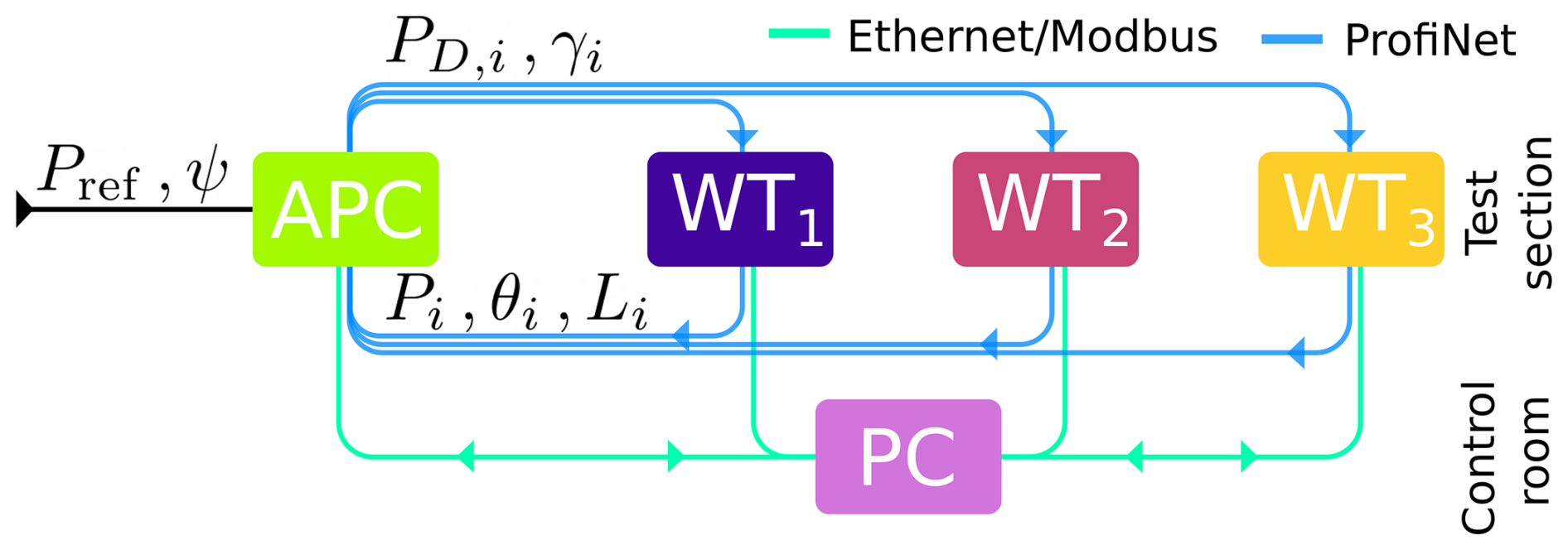
The maximum-reserve APC used in this work has been extensively described in Tamaro et al. (2025b), so here we only summarize its main features. The core of the wind farm control architecture is an open-loop model-based set-point optimal scheduler that determines the yaw misalignment and power demand of each turbine, given the power demand required by the TSO and the ambient conditions. Furthermore, a feedback loop serves the purpose of correcting tracking errors that may arise from the open loop in real time. A sketch of the controller is shown in Fig. 1.

Figure 1 Schematic representation of the maximum-reserve APC controller, featuring an open-loop model-based optimizer and a closed-loop corrector.

The closed and open loops are executed at two distinct time rates, since their outputs involve physical phenomena characterized by different time scales. Specifically, the open loop updates the yaw set-points γ_i and the power demand P_D at a slow pace, due to the time required by wakes to propagate downstream, whereas the closed-loop corrector acts at a rate that is 2 orders of magnitude faster.

2.1.1 Open-loop set-point optimal scheduler

The open-loop component of the algorithm provides the optimal set-points in terms of yaw misalignment and power share. These are computed by a gradient-based optimization that maximizes the smallest power reserve within the farm for a given overall power demand and ambient conditions.

Given the total number of turbines N in the farm, the power of the ith machine is noted as $P_i=P_i({\mathbf{A}}_i,{\mathit{u}}_i)$, where A_i indicates the ambient conditions. Ambient conditions here are assumed to include freestream wind speed U_∞, wind direction ψ, vertical shear k, and turbulence intensity (TI) I. The control inputs are noted as u_i, and they include the power share ${\mathit{\alpha }}_i=P_i/{\sum }_{i=\mathrm{1}}^N{P}_i$ and yaw misalignment γ_i.

The maximum power that can be generated by turbine i by adjusting its control set-points u_i (while keeping the set-points of the other turbines fixed) in the ambient conditions A_i is computed as

$${\displaystyle }{\displaystyle }{P}_{a,i}=\underset{{\mathit{u}}_i}{max}{P}_i({\mathbf{A}}_i,{\mathit{u}}_i)={\displaystyle \frac{\mathrm{1}}{\mathrm{2}}}\mathit{\rho }\mathit{\pi }{R}^{\mathrm{2}}{U}^{\mathrm{3}}{C}_{\mathrm{P}}{\mathit{\eta }}_P({\mathit{\gamma }}_i,{\mathit{\delta }}_i),$$

where ρ is the air density, C_P is the power coefficient, R is the rotor radius, U is the local rotor-equivalent wind speed, and η_P is the power scaling factor used by Tamaro et al. (2024a) to model power losses due to yaw γ and tilt δ. The local flow conditions at the rotor of a turbine, including U, are computed with an engineering flow model, here based on FLORIS (National Renewable Energy Laboratory, 2022). The use of a steady-state flow model is justified by the fact that – as also shown later in Sect. 3.2 – the wind direction time scales targeted by the controller are 1 order of magnitude larger than the propagation time of wake effects.

The power tracking method looks for the combination of set-points that produce the minimum possible maximum power ratio $P_i/P_{a,i}$ across all N turbines in the farm while satisfying the power demand of the TSO, P_ref. This tracking criterion can be expressed as

$$\begin{array}{}\text{(1a)}& {\displaystyle }& {\displaystyle }\underset{u}{min}\underset{i\in [\mathrm{1},N]}{max}{\displaystyle \frac{P_i}{P_{a,i}}},\text{(1b)}& {\displaystyle }& {\displaystyle }\text{such that}\sum _{i=\mathrm{1}}^N{P}_i=P_{\text{ref}}.\end{array}$$

In fact, the smaller the power ratio $P_i/P_{a,i}$, the larger the reserve $\mathrm{1}-P_i/P_{a,i}$ that is available to compensate against drops in the wind.

CL+MR improves tracking performance because it explicitly targets small reserves, which – when they are exhausted and generate saturations – are the main drivers of tracking deviations (Tamaro et al., 2025b). This formulation can be implemented by using induction control alone or in combination with wake steering, the latter case being considered here.

Equation (1) represents a constrained optimization problem. The optimization does not need to be performed in real time during operation. Rather, it is executed offline for a set of ambient conditions and levels of wind farm curtailment. Results are collected in a lookup table (LUT), which is then interpolated at runtime, similarly to what is routinely done for power-boosting wind farm control (Meyers et al., 2022), so that

$$\begin{array}{}\text{(2a)}& {\displaystyle }& {\displaystyle }{\mathit{\alpha }}_i={\mathit{\alpha }}_i(P_{\text{ref}},\mathit{\psi },U_{\mathrm{\infty }},k,I),\text{(2b)}& {\displaystyle }& {\displaystyle }{\mathit{\gamma }}_i={\mathit{\gamma }}_i(P_{\text{ref}},\mathit{\psi },U_{\mathrm{\infty }},k,I).\end{array}$$

2.1.2 Closed-loop corrector

The closed-loop corrector is taken directly from the work of van Wingerden et al. (2017). The corrector consists of a simple proportional-integral (PI) feedback loop that operates on the power tracking error, which arises from the open-loop component of the control structure. Its goal is to ensure that – as some turbines deviate from their respective demands – the reference power tracking signal is promptly corrected.

The tracking error Δ_P is defined as

$$\begin{array}{}\text{(3)}& {\displaystyle }{\displaystyle }{\mathrm{\Delta }}_P=P_{\text{ref}}-\sum _{i=\mathrm{1}}^N{P}_i.\end{array}$$

The control signal $P_{\text{ref}}^{\text{PI}}$ at time instant τ is defined as

$$\begin{array}{}\text{(4)}& {\displaystyle }{\displaystyle }{P}_{\text{ref}}^{\text{PI}}=K_{\text{APC}}^P{\mathrm{\Delta }}_{P,\mathit{\tau }}+K_{\text{APC}}^I\sum _{j=\mathrm{1}}^{\mathit{\tau }}{\mathrm{\Delta }}_{P,j},\end{array}$$

where $K_{\text{APC}}^P$ and $K_{\text{APC}}^I$ are the PI gains, and j is a time step counter. The wind farm is then required to track $P_{\text{ref}}+P_{\text{ref}}^{\text{PI}}$.

The PI gains are obtained with a tuning procedure based on the simple Simulink (The MathWorks, Inc., 2022) model described in Sect. 3.4. The controller features an anti-windup element on the integrator when all turbines are saturated, i.e., when S=N, where S denotes the number of saturated rotors. Furthermore, the integrator is reset in certain conditions, as described in Sect. 3.4. The gain scheduling based on the number of saturated turbines proposed by van Wingerden et al. (2017) is not used due to the small size of the farm considered here, which causes abrupt variations in the gains that can lead to instabilities. Instead, when a turbine saturates, its local power tracking error is redistributed equally among the non-saturated ones as proposed by Vali et al. (2019) and described in more detail in Sect. 2.4.

2.2 Reference APC formulations for performance comparison

We rely on three reference wind farm APC controllers to compare the performance of the maximum-reserve method, namely:

• Open-loop (OL). This simple approach assigns predetermined set-points α_i to each turbine, as fractions of the power demanded by the TSO, so that ${\sum }_{i=\mathrm{1}}^N{\mathit{\alpha }}_i=\mathrm{1}$. The set-points α_i are scheduled with the instantaneous wind direction, so that α_i=α_i(ψ) to account for different local power availabilities induced by wake impingements. The values α_i are computed with the FLORIS model (National Renewable Energy Laboratory, 2022), as described in Sect. 4.

• Closed-loop (CL). This method is the same as OL with the addition of the closed-loop PI corrector described in Sect. 2.1.2. Similarly to the OL method, the values α_i are scheduled with the instantaneous wind direction based on predictions from FLORIS.

• Closed-loop with load balance (CL + LB). This method consists of CL without the fixed scheduling of the power share set-points α_i. Instead, an additional PI loop is nested to distribute the set-points α_i with the goal of balancing loads within the wind farm (Vali et al., 2019). This coordinated load distribution (CLD) loop modifies the power share set-points to minimize the load-balancing error ΔL, which is defined as

  $$\begin{array}{}\text{(5)}& {\displaystyle }{\displaystyle }{\mathrm{\Delta }}_{L,i}=L_i-\stackrel{\mathrm{‾}}{L},\end{array}$$

  where L_i is the load of the ith turbine and $\stackrel{\mathrm{‾}}{L}=\frac{\mathrm{1}}{N-S}{\sum }_{i=\mathrm{1}}^{N-S}{L}_{i,\text{non-sat.}}$ is the average load in the farm. A PI power share distribution at time instant τ is computed as

  $$\begin{array}{}\text{(6)}& {\displaystyle }{\displaystyle }{\mathit{\alpha }}_{i,\mathit{\tau }}=K_{\text{CLD}}^P{\mathrm{\Delta }}_{L,i}+K_{\text{CLD}}^I\sum _{j=\mathrm{1}}^{\mathit{\tau }}{\mathrm{\Delta }}_{L,i,j},\end{array}$$

  where $K_{\text{CLD}}^P$ and $K_{\text{CLD}}^I$ are the PI gains.

  In this work, the tower-base fore-aft bending moment is chosen as the target load L. The PI gains of the CLD loop are tuned with the same Simulink model used for the APC loop, described in Sect. 3.4. As proposed by Gonzalez Silva et al. (2022), the mean load is computed considering only non-saturated turbines. Furthermore, the integrator is reset on all turbines in the event that all turbines reach saturation. In these conditions, the error Δ_L,i is null – since it is computed only with non-saturated turbines – and the integrator component lies at zero, until at least one turbine recovers from saturation. An anti-windup is finally added to the integrator of each turbine whenever the power share α exceeds unfeasible values.

It is important to mention that the set-points for CL+MR are computed using the same FLORIS version adopted for OL, CL, and CL+LB. This ensures that any discrepancy deriving from the steady-state model is present in each compared control approach. Furthermore, CL, CL+LB, and CL+MR feature the same PI control block described in Sect. 2.1.2, ensuring that the closed-loop element is also the same.

2.3 Wind turbine controller

The wind turbine controller is based on two regimes, namely below rated and rated. In below-rated conditions, blades lie at the optimal pitch angle, while the generator torque is scheduled with the rotor speed Ω to ensure that the tip speed ratio λ yields the maximum C_P. The rated condition occurs when Ω exceeds its rated value Ω_R. In this case, torque is fixed while pitch angle increases from its optimal value to limit the power output to P_R. Turbines can track a given power demand P_D (where P_D≤P_R) by adjusting Ω_R and by setting $Q_R=P_D/{\mathrm{\Omega }}_R$.

In this control strategy, the blade pitch angle θ serves as an indicator of the operating reserve – or margin – for a curtailed wind turbine (Tamaro and Bottasso, 2023). Typically, larger values of θ suggest a greater margin, as the turbine is functioning below its optimal power coefficient. The minimum (so called “fine”) value for θ corresponds to the optimal pitch angle θ_opt, which achieves the maximum C_P.

This controller was selected here because it directly accepts a power-demand input and uses the blade pitch angle to accurately follow it. Alternative control strategies could also be implemented, although they might lead to different APC performance.

2.4 Identification and treatment of saturation conditions

Saturations are detected on one turbine when the blade pitch lies at its optimal value plus a tolerance, and the tracking error exceeds a given threshold as specified in Sect. 3.1. When a wind turbine enters saturation, its power demand is set to $P_{\mathrm{D},i}^{*}$, which is the last value recorded before saturation, and its power share is computed as

$$\begin{array}{}\text{(7)}& {\displaystyle }{\displaystyle }{\mathit{\alpha }}_i={\displaystyle \frac{P_i}{P_{\text{ref}}+P_{\text{ref}}^{\text{PI}}}}.\end{array}$$

Then its local tracking error is equally redistributed to non-saturated turbines in the form of an additional power demand, in order to ensure that ${\sum }_{i=\mathrm{1}}^N{\mathit{\alpha }}_i=\mathrm{1}$. Notice that local isolated persistent saturation events do not necessarily introduce significant tracking errors as long as other turbines have enough margin to compensate.

Clearly, conditions in which all wind turbines are close to saturation are particularly harmful to the tracking accuracy, as a cascading effect can be triggered that may lead to all turbines being saturated. In this case, all wind turbines operate in greedy mode, and if the TSO demand drops, a large negative Δ_P will result. To avoid this situation, when the wind farm produces more than the instantaneous demand (with a threshold, as explained earlier), every saturation condition is forcibly reset.

3 Methods

3.1 Experimental set-up

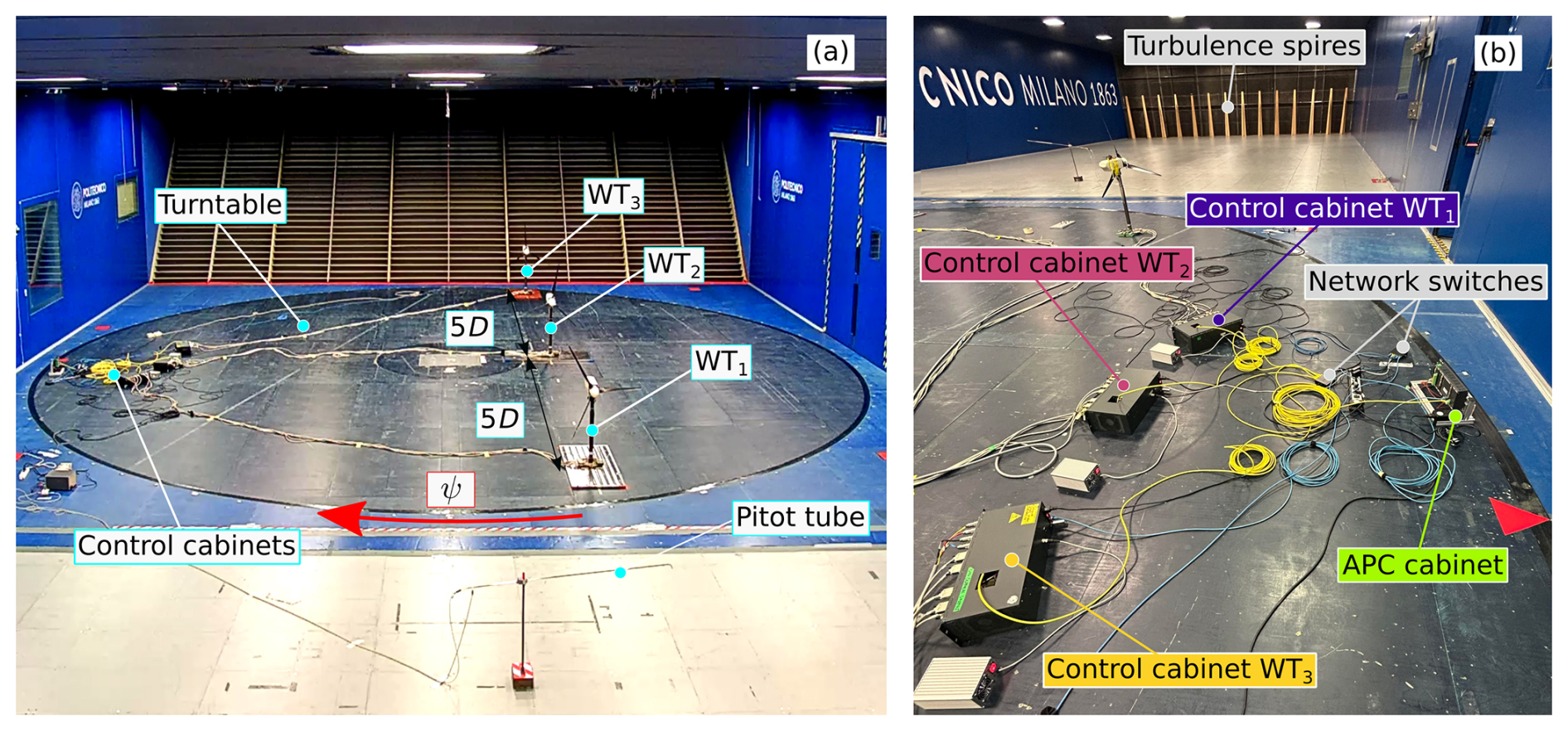
The wind tunnel experimental campaign is performed with a cluster of three G1 wind turbines (Bottasso and Campagnolo, 2022; Wang et al., 2021) – labeled WT₁ (upstream), WT₂ (center), and WT₃ (downstream) – longitudinally spaced by 5D, where D=1.1 m is the rotor diameter. The G1 scaled machine has a rated rotor speed Ω_R of 850 rpm, a rated power P_R of 46 W, an optimal collective blade pitch angle θ_OPT of 0.43°, and zero tilt. The time compression ratio is equal to about 80, which means that time flows much faster in the experiment than at full scale (Canet et al., 2021; Bottasso and Campagnolo, 2022). Each G1 is controlled in real time by a dedicated Bachmann M1 PLC (Bachmann electronic GmbH, 2017), which executes the turbine-level controller described in Sect. 2.3 every Δt=4 ms. The maximum yaw rate is equal to 20° s⁻¹, corresponding to approximately 0.25° s⁻¹ at full scale, which is a realistic value (Jonkman et al., 2009; Bortolotti et al., 2019).

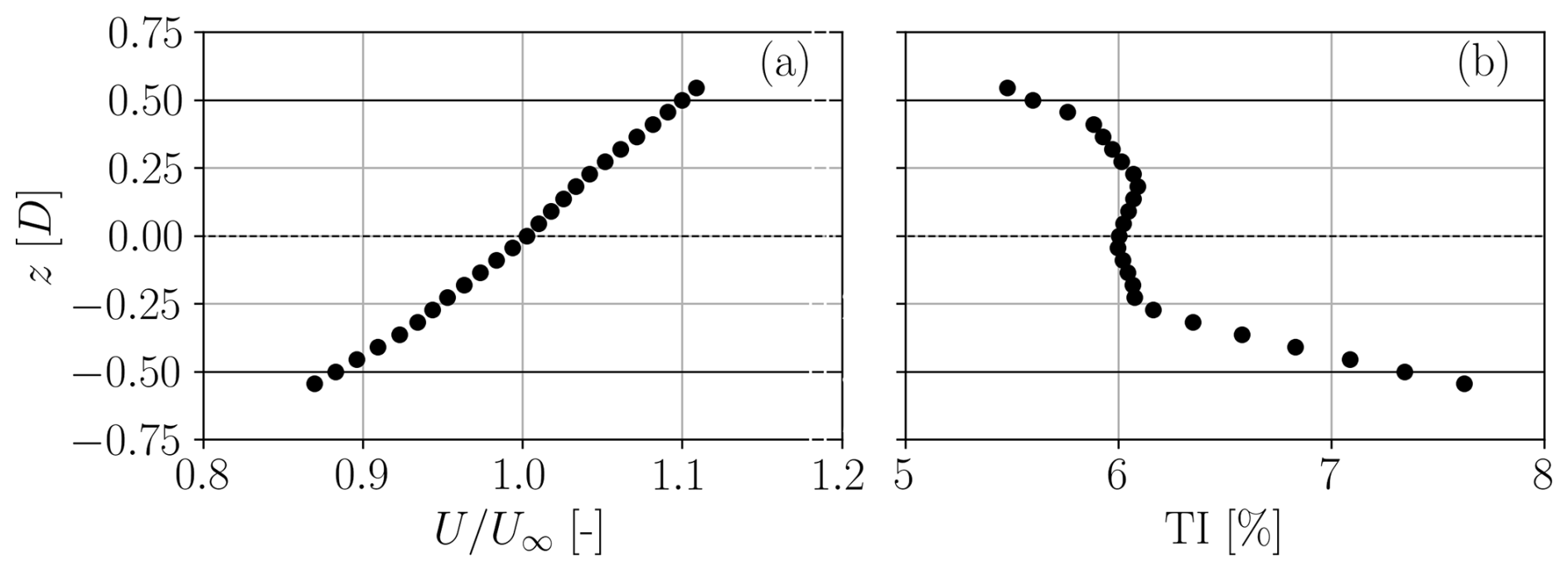
Tests are performed in the atmospheric test section of the wind tunnel of the Politecnico di Milano (Bottasso et al., 2014) in moderate turbulence conditions, with a power-law shear exponent k=0.14, a TI=6 % at hub height, and an integral length scale of turbulence of 0.79D. These ambient conditions are representative of offshore scenarios under neutral atmospheric boundary-layer conditions. It is important to recall that even a fairly mild freestream turbulence intensity results in very large turbulent fluctuations at downstream turbines, especially in such closely spaced configurations; for example, Fig. 11 of Tamaro et al. (2025b) shows wake-affected turbines experiencing TI values exceeding 30 % for a freestream TI of 5.7 %. Such high turbulence intensities create very challenging conditions for power tracking at downstream turbines.

The blockage ratio considering one G1 rotor is 1.8 %, which is significantly smaller than previous APC wind tunnel studies (Petrović et al., 2018; Gonzalez Silva et al., 2024). The three turbines are installed on a large turntable. The rotational speed of the wind tunnel fans is kept constant during the experiments. The resulting wind speed U_∞, measured by a pitot tube placed 4D upstream of WT₁, is approximately equal to 5.5 ms⁻¹.

Two sets of experiments are conducted, respectively referred to in the following as “static” and “dynamic”.

In the static tests, the turntable is fixed at an angle ψ to reproduce a specific wind direction. Two angles are considered, corresponding to partial rotor overlaps of 75 % (ψ=2.8°) and 50 % (ψ=5.7°), respectively. We define rotor overlap as the fraction (in percentage) of the diameter that two wind turbine rotors share when looking downstream. An overlap of 100 % corresponds to perfectly aligned rotors (center-to-center), while 50 % overlap means that the downstream rotor is laterally displaced by half a rotor diameter. In the static wind direction scenarios, each test has a duration of approximately 30 s, corresponding to about 4 h at full scale. Six repetitions are performed to reduce the uncertainties caused by the turbulent fluctuations of the flow.

In the dynamic tests, the turntable is rotated according to a predetermined time series, in order to dynamically vary the wind direction over the cluster of turbines. In this case, each test has a duration of 180 s, to match the overall duration of the static tests.

Figure 2 shows the wind tunnel set-up, while Fig. 3 shows the vertical profiles of the mean streamwise velocity and turbulence intensity measured at the location of the upstream turbine WT₁ for ψ=0°.

Figure 2 Wind tunnel set-up (a) and close-up view of the control cabinets (b).

Figure 3 Wind tunnel inflow. Vertical wind speed profile (a), vertical TI profile (b).

The APC algorithms are implemented in MATLAB Simulink (The MathWorks, Inc., 2022), from which C++ codes are exported, and later compiled and loaded onto a Bachmann M1 PLC (Bachmann electronic GmbH, 2017). At every time step, the APC controller receives information on the current power demand and, for each wind turbine, on its instantaneous power production, blade pitch angle, and tower-base fore-aft bending moment. Furthermore, the APC controller is also informed in real time about the current wind farm power demand P_ref and the current wind direction ψ. In one sampling period, the set-points of demanded power and nacelle yaw are computed by the APC controller and dispatched to each wind turbine. The direction of the wind relative to the farm is read from the turntable encoder. Therefore, its measurement can be considered exact up to the accuracy of this sensor. In the field, the knowledge of ψ is definitively more uncertain, due to the typically limited accuracy of the onboard anemometry system and the yaw encoder. The effects of wind direction uncertainties on wake steering performance were experimentally investigated by Campagnolo et al. (2020), using a very similar set-up as the one considered here.

The control cabinets executing the wind turbine and APC controllers are connected to a PC in the control room via the Ethernet. This PC is used to monitor the wind turbine sensors through a graphical user interface, to install and uninstall applications, to activate the wind farm controller, and to modify its settings as necessary. The Modbus communication protocol is used to start simultaneous data acquisitions, due to its compatibility with MATLAB. Communication between the APC and the wind turbine controllers is instead accomplished with Ethernet cables through the Profinet protocol (Profibus Nutzerorganisation e.V. (PNO), 2018). This system was chosen due to its relatively fast communication capabilities and integration with the existing set-up. The APC algorithms are executed with a time step of 4 ms (equivalent to approximately 0.3 s at full scale) to match the time step of the wind turbine controllers. In CL+MR, the open-loop scheduler is updated 100 times slower, i.e., every 0.4 s, corresponding to approximately 30 s at full scale. A sketch of the connections among the various components of the system is shown in Fig. 4.

Figure 4 Sketch of the wiring connections among wind turbines, APC, and PC.

Local saturation conditions are indicated by a flag that is raised when both of the following conditions are simultaneously verified:

• The tracking error of a turbine exceeds 1 % of the rated power P_R, i.e., 0.46 W, and

• Its blade pitch angle is lower than θ_OPT=0.37°.

Saturation conditions are also used to control the integral part of the APC PI controller. As discussed in Sect. 2.1.2, the integrator in the APC loop includes an anti-windup element that is activated when all turbines in the wind farm become saturated. This mechanism quickly reduces the integral term by applying to it a gain of 0.99 at each time step.

All saturation flags are reset when the wind farm power output exceeds P_ref by more than 3%P_R=1.38 W. This mechanism addresses the situation in which all turbines become saturated. In such cases, the rotors are commanded to follow $P_{\mathrm{D},i}=P_{\mathrm{D},i}^{*}$, i.e., the last demanded power value prior to saturation, as described in Sect. 2.4. However, when all turbines are saturated, the system is unable to detect changes in P_ref. Consequently, the machines would continue tracking $P_{\mathrm{D},i}^{*}$ even if P_ref decreases. To avoid this situation, the APC integrator and all saturations are reset whenever ${\mathrm{\Delta }}_P<-\mathrm{3}\mathit{\%}{P}_{\mathrm{R}}$. In the CLD PI controller, the integrator is reset either when all turbines become saturated or when this condition ends.

The control algorithms rely on multiple first-order filters. Cut-off frequencies are normalized using the rated rotor speed Ω_R, which allows for a straightforward conversion to the full-scale case. For all controllers described in Sect. 2, the power generated by each turbine is low-pass filtered using a first-order transfer function with a cut-off frequency of 5 Hz (=0.35 Ω_R), before inputting it in the farm-level controller. A first-order filter is chosen here to limit the time delay associated with higher-order filters, which would hinder tracking accuracy. A cut-off frequency of 1.57 Hz ($=\mathrm{0.11},{\mathrm{\Omega }}_R$) is used to update the power set-points, while a lower cut-off of 0.72 Hz (=0.05 Ω_R) is employed for the power demand. These different cut-off frequencies are selected to ensure that the power-demand signal remains smooth while minimizing delays in the set-points.

For CL+LB, fore-aft bending moments are filtered using a moving average with a fundamental frequency of 1 Hz (=0.07 Ω_R). This value is 1 order of magnitude smaller than the turbine first fore-aft mode at 16 Hz, thereby ensuring that the controller detects only mean loads and does not react to structural vibrations.

3.2 Turntable control

The wind tunnel turntable has a diameter of 13 m, and it can be rotated to follow a prescribed time history (Campagnolo et al., 2020). The time series has been sampled at 1 Hz at an onshore test site in northern Germany (Bromm et al., 2018) and scaled by the speed-up factor of the experiment. Campagnolo et al. (2020) have extensively discussed this set-up, showing a good agreement between the wind direction dynamics in the field and in the lab. Figure 5 reports the tunnel-scaled direction time history ψ(t).

Figure 5 Time history of wind direction ψ(t). Full rotor alignments (ψ=0°) are highlighted.

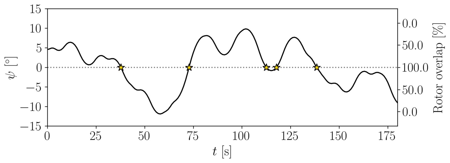
The figure shows that the scaled time history mainly consists of fluctuations characterized by slow frequencies f_ψ≤0.05 Hz. These correspond to time scales longer than 20 s, which are 1 order of magnitude larger than the 1–2 s characterizing the propagation time of wake effects. Clearly, the same conclusions would apply at full scale. This also justifies the adoption of a steady-state wake model for the synthesis of the controller.

Throughout the experiment, the wind direction changes sign five times. This condition is particularly challenging when performing double-sided wake steering since it requires a sudden, large yaw angle variation to change the side where wakes are deflected.

Figure 6a presents the measured available farm power as a function of wind direction ψ, while Fig. 6b shows the measured variation of local power share as a function of ψ in the absence of wind farm control (i.e., in standard greedy mode).

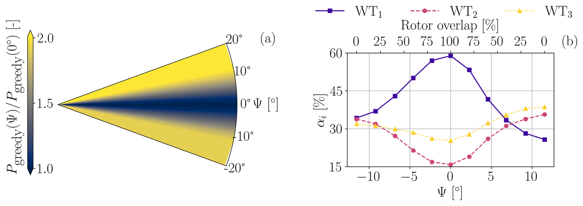
Figure 6 (a) Non-dimensional available power $P_{\text{greedy}}\left(\mathit{\psi }\right)/P_{\text{greedy}}\left(\mathrm{0}\mathit{°}\right)$ as a function of wind direction ψ. (b) Local power set-points as functions of ψ in greedy mode. When ψ=0°, the wind turbines are fully aligned.

Figure 6a highlights the strong effect of wake impingement on power production. The minimum available power is visible in correspondence with ψ≈0°. The lack of symmetry with respect to ψ is due to a lateral inhomogeneity of the flow within the wind tunnel (Campagnolo et al., 2020). Overall, WT₂ appears to be suffering the most significant power losses, as in fact it produces only 15 % of the wind farm power when ψ=0°. WT₃ presents a slightly higher power due to the high turbulence in the two wakes that impinge on it, which speeds up their recovery.

3.3 Reference power-demand signal

A dynamic reference power signal typical of automatic generation control (AGC) is used as an input signal to the farm-level tracking controllers. AGC is the secondary response regime of grid frequency control, and it consists of dynamically adjusting the power output of a plant according to the request of the TSO (Aho et al., 2012). A similar signal has been considered by other authors (Fleming et al., 2016; van Wingerden et al., 2017; Vali et al., 2019; Shapiro et al., 2017; Boersma et al., 2018). The signal is defined as

$$\begin{array}{}\text{(8)}& {\displaystyle }{\displaystyle }P(t,\mathit{\psi })=P_{\text{greedy}}\left(\mathit{\psi }\right)\left(b+c{n}_k^{\text{AGC}}\left(t\right)\right),\end{array}$$

where $n_k^{\text{AGC}}\left(t\right)$ is a normalized time-dependent test signal, P_greedy(ψ) is the available power of the wind farm in greedy aligned conditions at a specific wind direction ψ, and b and c are two parameters that respectively shift and scale $n_k^{\text{AGC}}$.

Due to the small size of the models, the original signal is accelerated in time by a factor of 81.73 (Bottasso and Campagnolo, 2022). Figure 7a shows $n_k^{\text{AGC}}$ as a function of time. In the tests with the dynamic turntable, the reference power signal in Fig. 7a is looped multiple times for a total length of 3 min. In this case, the instantaneous available wind farm power P_greedy(ψ) depends on the instantaneous wind direction ψ as shown in Fig. 6a. Figure 7b shows the time history of $n_k^{\text{AGC}}\left(t\right)P_{\text{greedy}}\left(\mathit{\psi }\right)/P_{\text{greedy}}\left(\mathrm{0}\mathit{°}\right)$, where both the full-scale (top x axis) and wind tunnel (bottom x axis) time scales are reported.

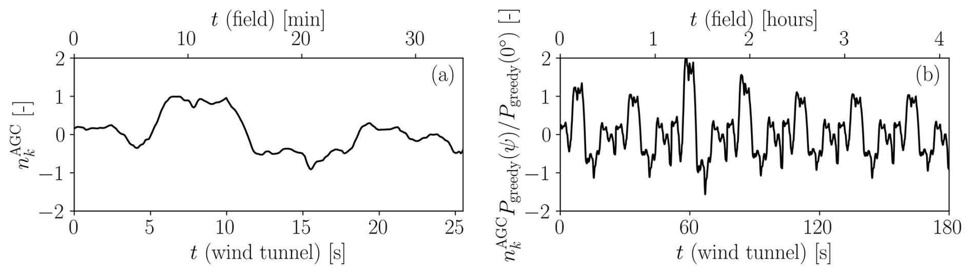
Figure 7 Time series of the reference test signal $n_k^{\text{AGC}}$ (a) and of the normalized power reference used in the dynamic turntable experiments (b). The additional x axis on the top part of the plot indicates full-scale time.

The reference power signal is initialized with a rising ramp to reduce the effects of initial transients. Notice how a 4 h long test in the field is replicated in the significantly shorter time of 180 s in the wind tunnel. It is important to notice that the test time of 3 min covers 24 full-scale 10 min turbulent realizations, which ensures the statistical convergence of results (Liew and Larsen, 2022).

3.4 Tuning procedure of the PI gains

The gains used in the APC controllers and the cut-off frequencies of the filters are tuned using a digital twin of the wind tunnel set-up. This model of the experiment is implemented in Simulink (The MathWorks, Inc., 2022) and includes three blocks representing the wind turbines, each running the same controller used in the wind tunnel tests. The drivetrain dynamics are modeled as described in Campagnolo et al. (2022a), while rotor aerodynamics are represented using LUTs computed offline with a blade element momentum (BEM) model of the G1 (Wang et al., 2020). The LUTs schedule rotor thrust and torque as functions of turbine operating conditions. Tower dynamics are modeled with a second-order system.

The Jensen wake model (Jensen, 1983), combined with the instantaneous thrust coefficient C_T, is used to estimate the wake deficit for downstream turbines. A delay is used to simulate the time required for wake effects to propagate downstream. The same CL and CL+LB controllers used in the wind tunnel experiments are included in the digital twin. To improve the robustness of gain tuning, zero-mean white noise with a variance of 0.25 W² is added to the measured input power.

Gain optimization is performed with the goal of reducing the influence of saturation events, using a gradient-based interior-point algorithm with a power-demand signal characterized by P_greedy=55 W, b=0.8, and c=0.1.

For the CL+LB controller, the cost function is defined as

$$\begin{array}{}\text{(9)}& {\displaystyle }{\displaystyle }J=\mathrm{0.75}{\stackrel{\mathrm{‾}}{\mathrm{\Delta }}}_P+\mathrm{0.25}\sum _{i=\mathrm{1}}^N{\stackrel{\mathrm{‾}}{\mathrm{\Delta }}}_{L,i},\end{array}$$

which represents a weighted sum of the non-dimensional tracking error ${\stackrel{\mathrm{‾}}{\mathrm{\Delta }}}_P$ and the non-dimensional load-balancing error ${\stackrel{\mathrm{‾}}{\mathrm{\Delta }}}_{L,i}$. Both quantities are scaled to lie in the interval [0,1].

The resulting gains for the APC loop are

$$\begin{array}{ll}{\displaystyle }& {\displaystyle }{K}_{\text{APC}}^P=\mathrm{1.3127}\text{ [–] },\\ {\displaystyle }& {\displaystyle }{K}_{\text{APC}}^I=\mathrm{14.9253}{\mathrm{s}}^{-\mathrm{1}}=\mathrm{1.05}{\mathrm{\Omega }}_R.\end{array}$$

For the CLD loop, the gains are

$$\begin{array}{ll}{\displaystyle }& {\displaystyle }{K}_{\text{CLD}}^P=\mathrm{0.03427}{\text{Nm}}^{-\mathrm{1}}=\mathrm{0.52}{L}_R^{-\mathrm{1}},\\ {\displaystyle }& {\displaystyle }{K}_{\text{CLD}}^I=\mathrm{0.07959}{\text{Nm}}^{-\mathrm{1}}{\mathrm{s}}^{-\mathrm{1}}=\mathrm{0.09}{L}_R^{-\mathrm{1}}{\mathrm{\Omega }}_R,\end{array}$$

where L_R=15.2 Nm is the tower-base fore-aft bending moment of the G1 turbine at rated wind speed.

4 Steady-state performance characterization

The engineering farm flow model FLORIS v3 (National Renewable Energy Laboratory, 2022) is used here to perform a steady-state characterization of the performance of the various controllers, before entering the wind tunnel. The same model is also used to synthesize the open-loop part of the controller, yielding the control LUTs.

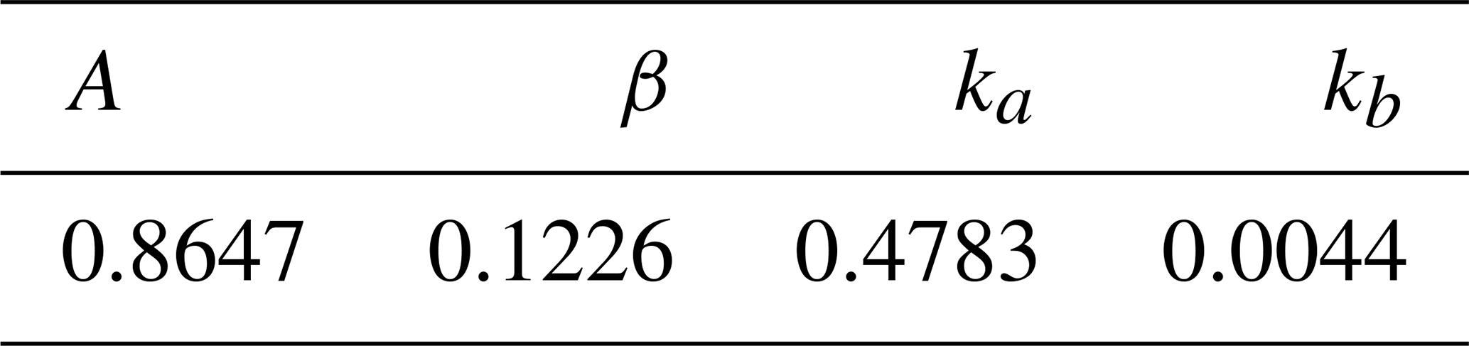
The wake deficit and deflection models proposed by Bastankhah and Porté-Agel (2014) are employed, along with the turbulence model by Crespo and Hernàndez (1996). In both cases, the model parameters are fine-tuned to replicate wind tunnel conditions, as summarized in Appendix A.

FLORIS is also augmented with a heterogeneous wind map that replicates the asymmetric inflow of the wind tunnel shown in Sect. 3.2 (Campagnolo et al., 2022b), following the procedure proposed by Braunbehrens et al. (2023). In OL and CL, the same engineering flow model is used to assign the power share set-points α_i as functions of ψ, given the ambient conditions of the experiments.

4.1 Set-points for CL+MR: combining wake steering with off-rated operation

In CL+MR, wind turbines are subjected to induction control and simultaneously perform wake steering. To model this combined off-rated and misaligned operation, LUTs of power coefficient C_P and thrust coefficient C_T are computed via an analytical model (Tamaro et al., 2024a). The adoption of such a model is motivated by the fact that off-rated operation spans a wide range of C_T values – and misaligned operation is strongly dependent on C_T (Cossu, 2021; Heck et al., 2023).

Another important aspect typical of scaled wind turbine models is the effect of the chord-based Reynolds number on the aerodynamic performance of the rotor (Bottasso and Campagnolo, 2022). This is relevant since with the controller described in Sect. 2.3, turbines operating in off-rated conditions experience low rotational speeds. These effects were taken into account by using a BEM model of the G1 that includes a dependency on the chord-based Reynolds number (Wang et al., 2020). Figures 8 and 9 show examples of LUTs for C_P and C_T, where the auxiliary factor ϵ has been introduced to quantify the level of derating, with ϵ=1 corresponding to the greedy power mode.

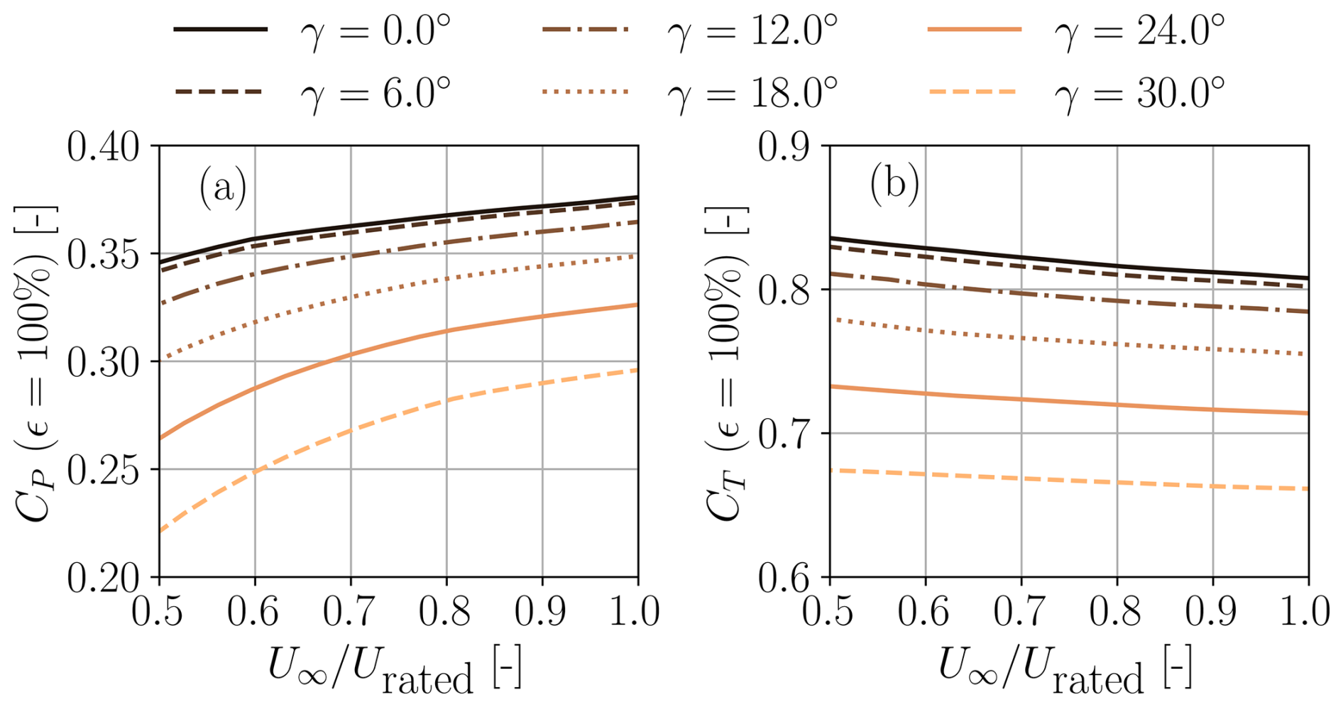
Figure 8 LUTs for (a) power coefficient C_P and (b) thrust coefficient C_T as functions of wind speed for the G1 turbine. Results corresponds to a power scaling factor ϵ=100 %, (i.e., no curtailment) and different yaw angles γ.

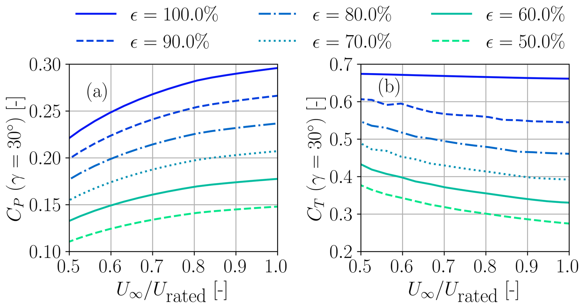
Figure 9 LUTs for (a) power coefficient C_P and (b) thrust coefficient C_T as functions of wind speed for the G1 turbine. Results correspond to a yaw angle γ=30° and different power scaling factors ϵ, representing the level of power curtailment.

Since both power demand and wind direction vary, the LUTs for γ_i(P_D,ψ) and α_i(P_D,ψ) are two-dimensional. Other model inputs, such as TI and inflow shear, are fixed as described in Sect. 3.1. To generate the LUTs, different optimizations are solved for each wind direction and wind farm power demand. When the optimization converges, the resulting power share set-points are computed as ${\mathit{\alpha }}_i=P_i/{\sum }_{i=\mathrm{1}}^N{P}_i$, and they are stored together with the yaw set-points. The optimization problem is solved with the gradient-based sequential quadratic programming (SQP) method (Brayton et al., 1979). With the aim of avoiding entrapment in local minima, the optimization for the first power-demand level is carried out using various random perturbations of the power-boosting solution as initial guesses. After this first solution, the wind farm power demand is progressively lowered and the result of the previous optimization is used as a starting guess for the next curtailment level. The minimum curtailment levels is limited to 40 % of the maximum wind farm power, which is sufficient to cover the APC scenarios described in Sect. 3.3. Results are shown in Figs. 10 and 11 for the yaw and power set-points, respectively.

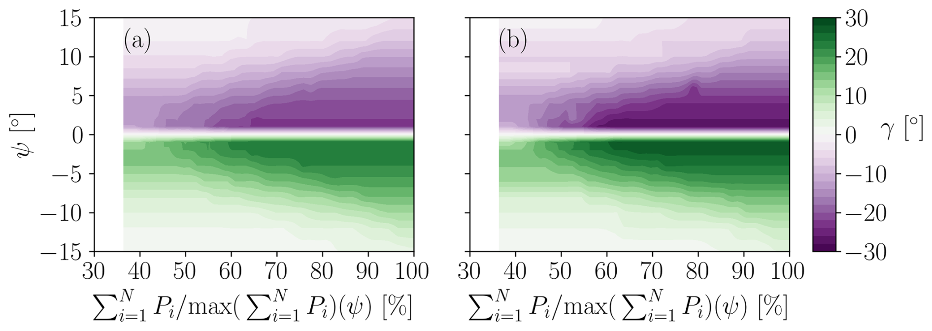
Figure 10 Optimal yaw set-points γ that maximize the minimum power reserve for the experimental set-up, plotted against the power demanded to the wind farm in percentage of the maximum power, and the inflow wind direction ψ. (a) WT₁, (b) WT₂.

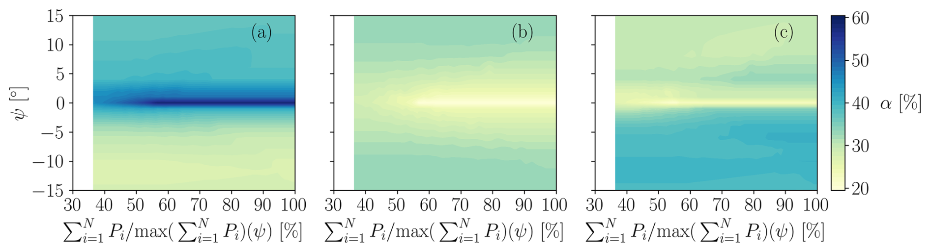
Figure 11 Optimal power set-points α that maximize the minimum power reserve for the experimental set-up, plotted against the power demanded to the wind farm in percentage of the maximum power, and the inflow wind direction ψ. (a) WT₁, (b) WT₂, (c) WT₃.

In the figures, ψ=0° represents a condition of precise alignment and therefore full wake impingement. Conversely, when $\mathrm{0}\mathit{°}<\left|\mathit{\psi }\right|\le \mathrm{11.3}\mathit{°}$, partial wake impingement occurs. The yaw set-points present, in fact, a maximum absolute value in full waking, where steering is heavily used to increase power reserves. As ψ increases, the power set-points start converging toward an equal power dispatch, i.e., ${\mathit{\alpha }}_i=\mathrm{1}/N$, while the yaw misalignment is progressively reduced. In fact, as ψ deviates away from 0°, wake impingement is less prominent, and all turbines perceive similar local inflow conditions.

The treatment of the ψ=0° condition is particularly relevant: under dynamic wind direction variations, when ψ switches sign, the upstream wind turbines must change their yaw set-point by more than ±40°. Delays in following this demand – which are expected due to the necessarily limited speed of the yaw actuation system – could result in relevant power losses, since the wake may be temporarily deflected toward downstream rotors, instead of away from them. To avoid this situation, no optimal wake steering is performed between $-\mathrm{2}\mathit{°}<\mathit{\psi }<\mathrm{2}\mathit{°}$, but instead, the set-points are interpolated from the values at ±2° to ensure a smooth transition when ψ switches sign. This solution should not result in a hindrance to the overall effectiveness of wake steering, since deflecting wakes is more effective in partial than in full impingement (Howland et al., 2019).

During operation, α_i and γ_i are linearly interpolated from the LUTs in Figs. 10 and 11 based on the average power demand and wind direction computed over the previous 0.4 s. Clipping to the last available value of the LUT is used to avoid extrapolating.

4.2 Estimation of the power margins

The power reserves for CL+MR are compared to those of OL in steady-state conditions, using the simulation environment described earlier. The comparison considers the difference between the power-produced P_i and the available power P_a,i for each turbine. Figure 12 shows the locally available power and the minimum power (last column) in the farm for two wind directions, i.e., ψ=2.8 and 5.7°, corresponding to partial rotor overlaps of 75 % and 50 %, respectively.

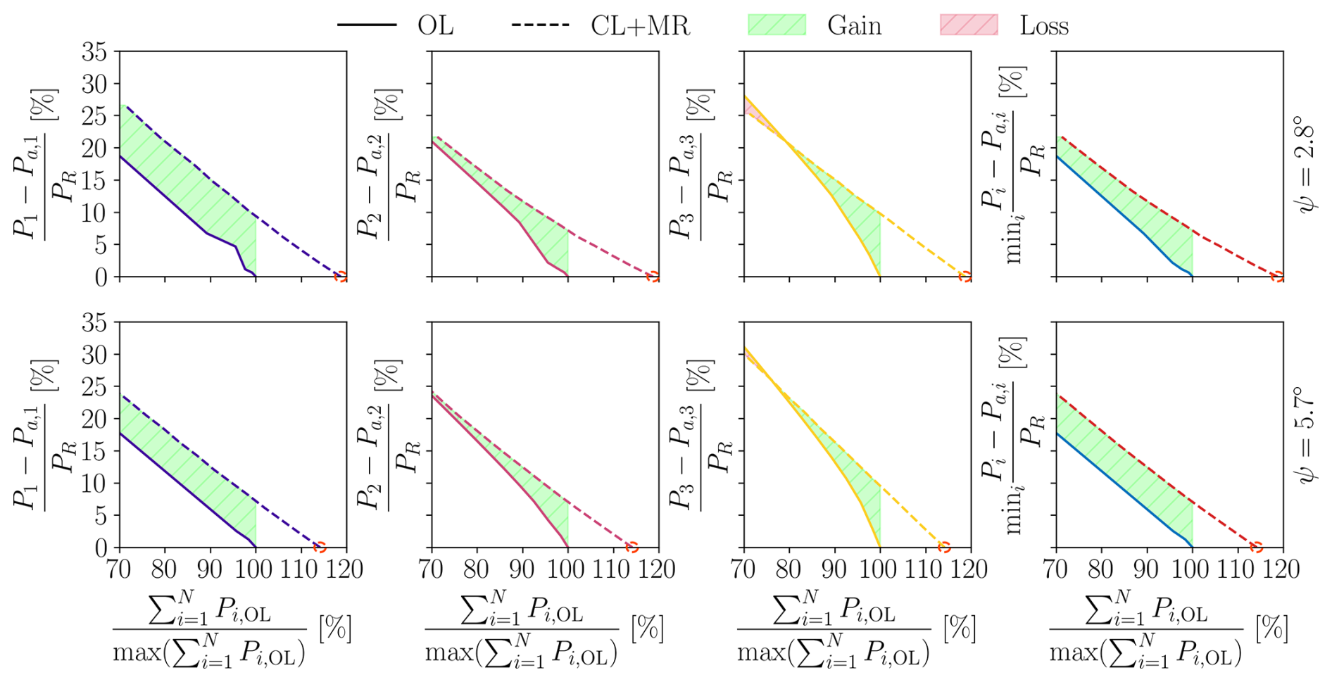
Figure 12 Locally available power normalized with the rated power P_R, obtained with a purely inductive wind farm control (labeled OL) and with the maximum-reserve strategy (labeled CL+MR) for ψ=2.8° and ψ=5.7°. (a) WT₁, (b) WT₂, (c) WT₃, (d) minimum value in the wind farm. On the x axis, the wind farm power is normalized with its maximum value without wake steering. Red circles indicate the classical maximum power solution.

Results show that the largest wind farm power gain is obtained for ψ=2.8° ($\approx +\mathrm{18}\mathrm{\%}$), followed by ψ=5.7° ($\approx +\mathrm{14}\mathrm{\%}$), confirming that wake steering is particularly beneficial in partial wake impingement conditions (Howland et al., 2019). As a result of the higher wind farm power, a significant gain in power reserve is achieved with CL+MR relative to OL, in particular for the front turbine WT₁. This is favorable, since WT₁ is often required to compensate for the saturations that may affect waked rotors. For these downstream turbines, the benefit of CL+MR becomes evident at severe power demands, i.e., ${\sum }_{i=\mathrm{1}}^N{P}_{i,\text{OL}}\approx \mathrm{95}\mathrm{\%}$, and it gradually decreases as ${\sum }_i{P}_{i,\text{OL}}$ is reduced because of the loss of effectiveness of wake steering due to the lower operational C_T of upstream rotors. This, in fact, implies a lower velocity deficit in the wake and a less prominent deflection. Overall, CL+MR yields a distribution of power reserves across the turbines that is more uniform than when using the OL method, consistently with the goal of the optimization.

The last two plots on the right in Fig. 12 show the worst power reserve in each cluster across the range of wind farm power demands for the two considered wind directions. For OL, WT₁ is the most critical rotor. Under curtailment, its power reserve increases linearly, albeit at a slower rate than that of the downstream rotors, which exhibit a non-linear increase (as shown in the corresponding plots, appearing in the second and third column of the figure), likely due to wake effects. In contrast, for CL+MR, the worst power reserve shifts from WT₁ to WT₂ as the rotors adjust their yaw alignment, in turn resulting in consistently larger margins than in the OL case.

5 Static wind direction experiments

In this section, we present the wind tunnel results for two fixed wind direction values equal to ψ=2.8 and 5.7°, corresponding to partial rotor overlaps of 75 % and 50 %, respectively.

5.1 Power tracking accuracy

5.1.1 Wind farm tracking errors

Figures 13 and 14 present the root mean square (RMS) of the power tracking error recorded at the three power request levels b=0.8, 0.85, 0.9, by each APC algorithm in the wind tunnel experiments. For each controller, six measurements are shown, indicating six repetitions, and whiskers indicate the mean RMS error and its uncertainty considering a 95 % confidence level. Figure 13 presents the RMS of tracking error obtained for ψ=2.8°, while Fig. 14 refers to the case ψ=5.7°.

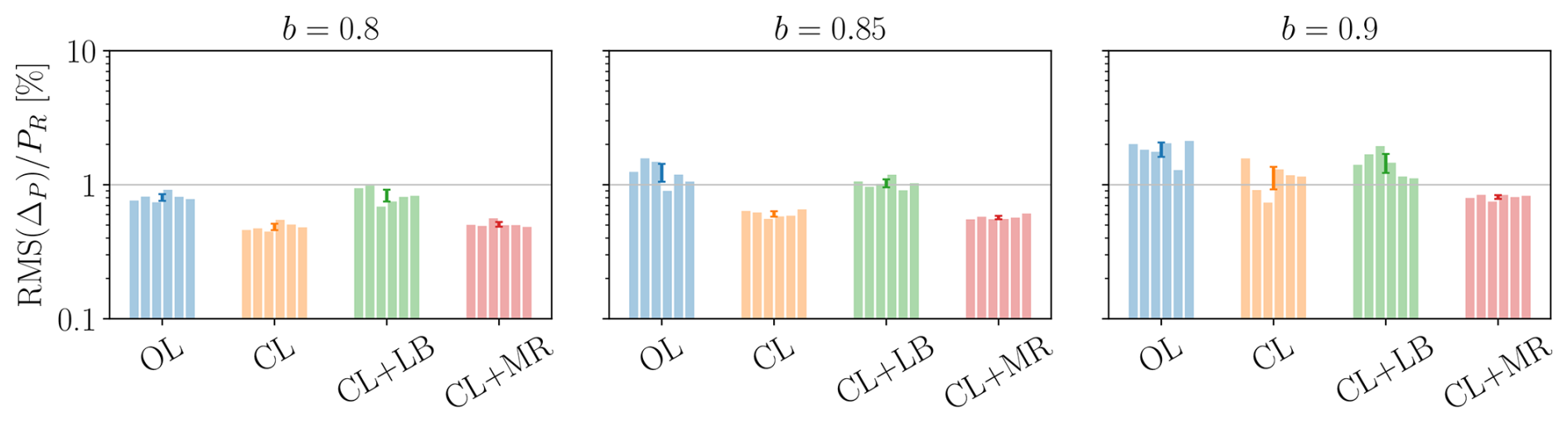
Figure 13 RMS of wind farm power tracking errors measured for the four APC algorithms and three power-demand levels b. Static experiment with fixed wind direction ψ=2.8°, corresponding to 75 % rotor overlap. The results from six repetitions are reported with bars for each APC algorithm and power demand. Whiskers indicate 95 % confidence intervals.

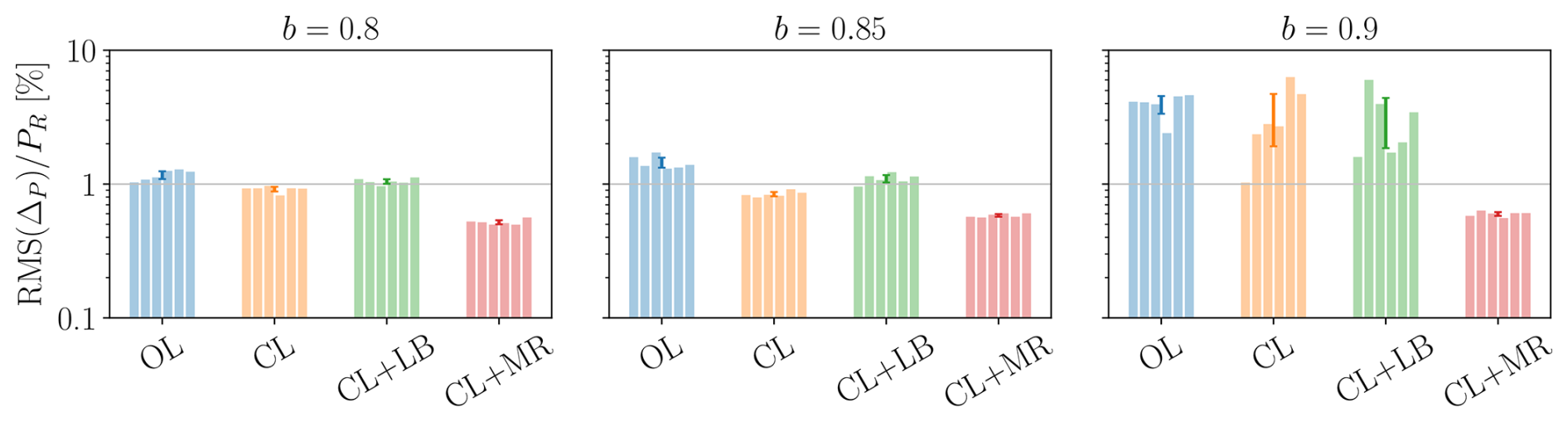
Figure 14 RMS of wind farm power tracking errors measured for the four APC algorithms and three power-demand levels b. Static experiment with fixed wind direction ψ=5.7°, corresponding to 50 % rotor overlap. The results from six repetitions are reported with bars for each APC algorithm and power demand. Whiskers indicate 95 % confidence intervals.

The plots show that the tracking error grows with the power request determined by parameter b. Closed-loop methods reduce the tracking error consistently, with a generally larger effectiveness for ψ=2.8°, i.e., for the higher rotor overlap case. Interestingly, the variability of the results increases significantly as parameter b grows in all cases except for CL+MR. The smaller variability observed for CL+MR is likely due to larger power reserves, which reduce the likelihood of simultaneous saturation events that can dramatically affect tracking accuracy.

5.1.2 Wind turbine tracking errors

Figures 15 and 16 show the tracking RMS error of each wind turbine for various power-demand levels, for ψ=2.8° and ψ=5.7°, respectively.

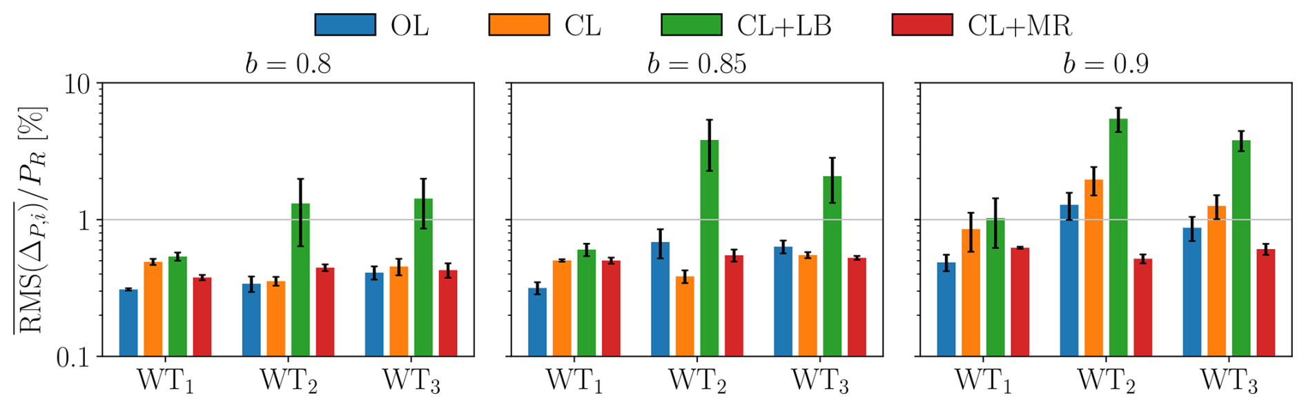
Figure 15 RMS of local power tracking errors for the four APC algorithms and three power-demand levels b. Static experiment with fixed wind direction ψ=2.8°, corresponding to 75 % rotor overlap. Whiskers indicate 95 % confidence intervals.

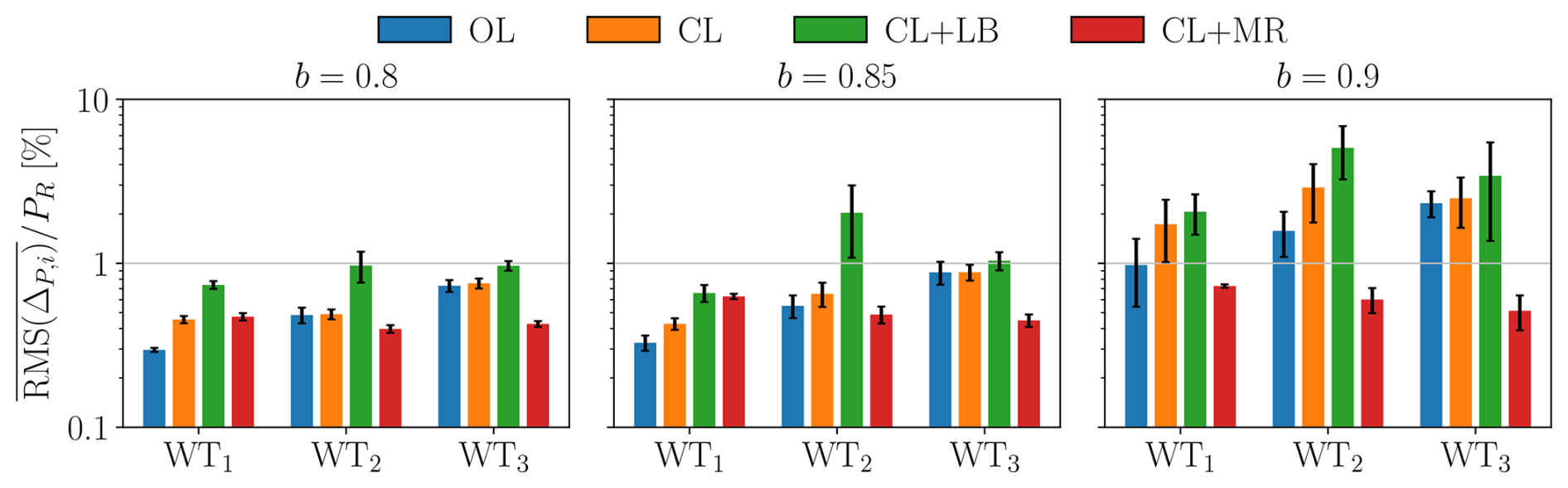
Figure 16 RMS of local power tracking errors for the four APC algorithms and three power-demand levels b. Static experiment with fixed wind direction ψ=5.7°, corresponding to 50 % rotor overlap. Whiskers indicate 95 % confidence intervals.

In the OL and CL+LB cases, waked rotors present the highest tracking error. In both cases, this is due to the generally low power reserves of waked rotors, which is exacerbated by the lack of a closed loop for OL and by the coordinated load distribution for CL+LB. Compared to OL, CL increases the tracking errors of WT₁ because it calls this front turbine that is operating in freestream to compensate for the saturation of the waked turbines further downstream. CL+MR presents a consistently balanced error distribution. This is likely due to the rather uniform distribution of power reserves, which implies that all turbines have a similar likelihood of not being able to follow a local demand.

It should be remarked that for all methods except for OL, a saturated turbine will experience significant tracking errors. This does not necessarily imply a low wind farm tracking accuracy but only as long as other turbines are able compensate. Therefore, it is important to ensure that local power reserves are not exhausted, which is precisely what the maximum-reserve formulation tries to accomplish.

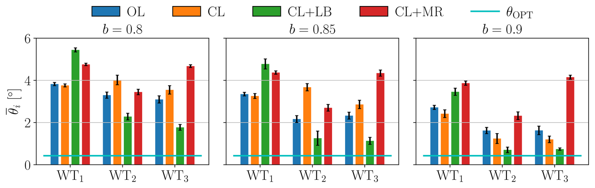
Figure 17 Local average blade pitch angle $\stackrel{\mathrm{‾}}{\mathit{\theta }}$ from the static turntable experiment for wind direction ψ=2.8°, corresponding to a 75 % rotor overlap. Whiskers indicate 95 % confidence intervals. Results are presented for three power-demand levels b.

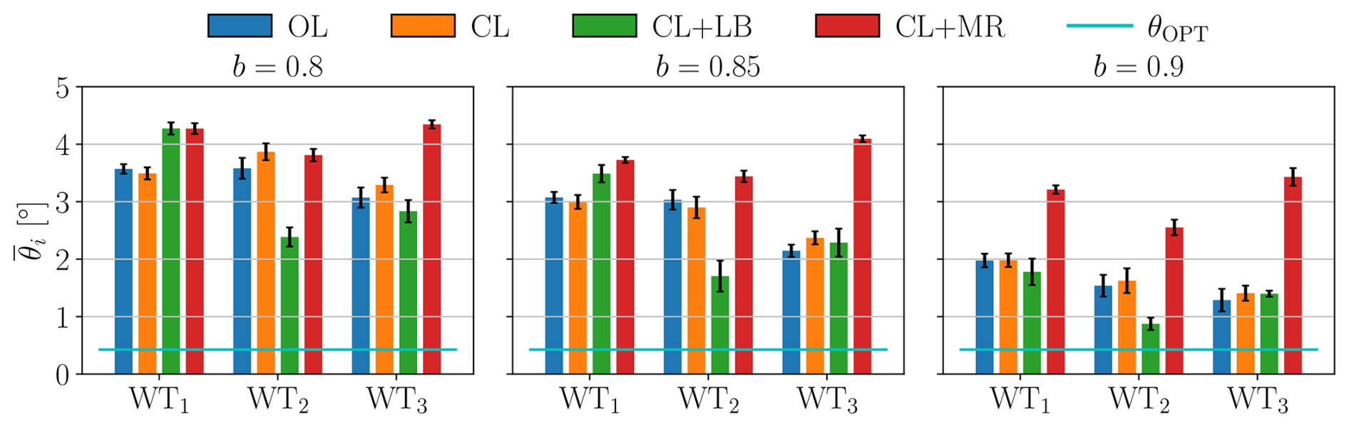
Figure 18 Local average blade pitch angle $\stackrel{\mathrm{‾}}{\mathit{\theta }}$ from the static turntable experiment with wind direction ψ=5.7°, corresponding to a 50 % rotor overlap. Whiskers indicate 95 % confidence intervals. Results are presented for three power-demand levels b.

5.2 Power reserve distribution

To quantify the mean power reserve of each turbine, we analyze the average collective blade pitch angle $\stackrel{\mathrm{‾}}{\mathit{\theta }}$. With the controller described in Sect. 2.3, the closer $\stackrel{\mathrm{‾}}{\mathit{\theta }}$ is to the optimal pitch θ_OPT, the less power reserve is available. Figures 17 and 18 show the local mean collective blade pitch angle for ψ=2.8° and ψ=5.7°, respectively.

Consistently with the tracking error analysis, $\stackrel{\mathrm{‾}}{\mathit{\theta }}$ appears to decrease as the power demand increases. OL and CL+LB present a power reserve distribution that is significantly unbalanced toward WT₁. In particular, CL+LB presents the highest values of $\stackrel{\mathrm{‾}}{\mathit{\theta }}$ for WT₁, but at the same time it also always yields low values of $\stackrel{\mathrm{‾}}{\mathit{\theta }}$ for waked rotors. CL remarkably improves the balancing of power reserves compared to OL, especially for ψ=2.8° and for low values of b. CL+MR presents a rather uniform distribution of the power reserves, favoring especially the most waked rotor, i.e., WT₃. This directly confirms the effectiveness of wake steering, which, by laterally moving upstream wakes, improves the power reserve of the most downstream rotor.

5.3 Loads and fatigue

In the following loads and fatigue analysis, we only display data for the 75 % rotor overlap scenario, since results for ψ=5.7° (50 % rotor overlap) are similar (and reported, for completeness, in Appendix C).

The mean local load-balancing error of each rotor is shown in Fig. 19.

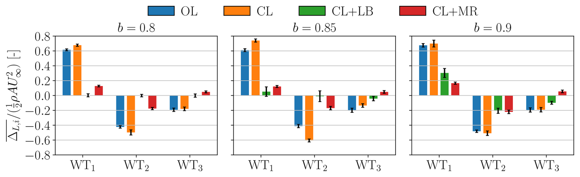
Figure 19 Mean local load-balancing error for the tower-base fore-aft bending moment for the static turntable experiment with wind direction ψ=2.8°, corresponding to a 75 % rotor overlap. L is normalized by $\frac{\mathrm{1}}{\mathrm{2}}\mathit{\rho }{U}_{\mathrm{\infty }}^{\mathrm{2}}$. Positive values indicate loading above the wind farm average. Whiskers indicate the mean error over six repetitions and its uncertainty considering a 95 % confidence level. Results are presented for three power-demand levels b.

Results show that for OL and CL, loading is maximum on WT₁ and decreases when moving downstream. CL+LB effectively balances loads in the wind farm, with remarkable effectiveness for b<0.9. When b=0.9, the significant increase in saturation events is such that loads cannot be balanced anymore, since power tracking accuracy is prioritized. This shows the limit of the load-balancing strategy that, in some cases, is unable to achieve the goals for which it has been formulated.

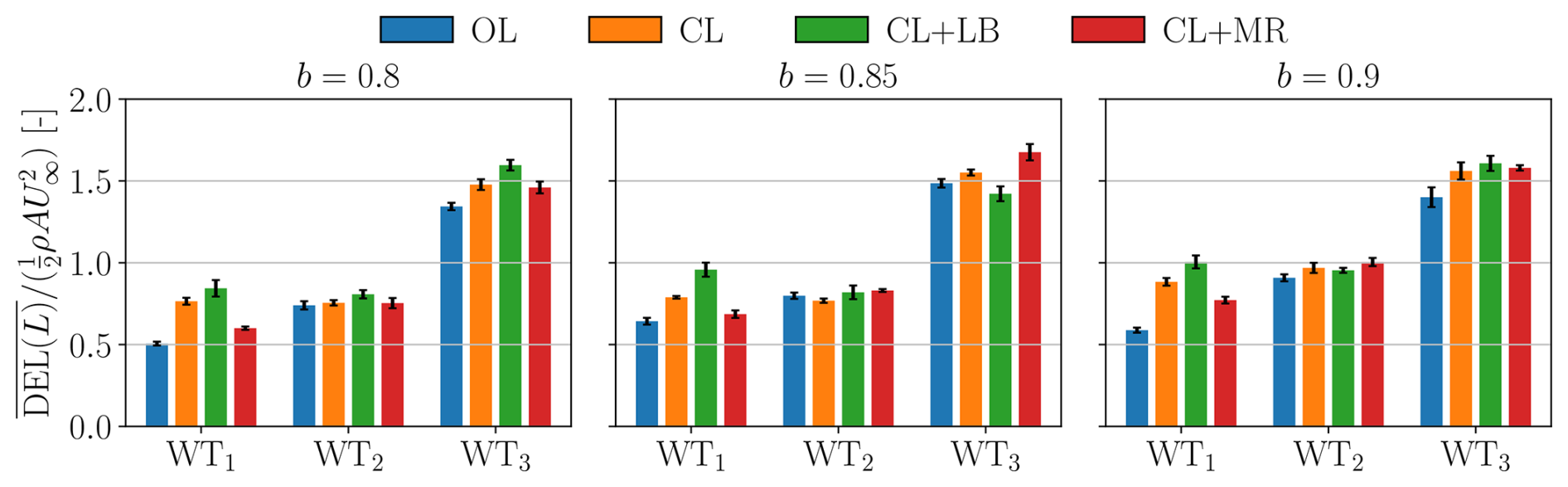
Figure 20 Normalized tower-base fore-aft DELs from the static turntable experiment for a wind direction ψ=2.8°, corresponding to 75 % rotor overlap. Whiskers indicate the mean DEL over six repetitions and its uncertainty considering a 95 % confidence level. Results are presented for three power-demand levels b.

Next, damage equivalent loads (DELs) at tower base are presented in Fig. 20.

Results show that waked turbines generally suffer more damage than those operating in freestream conditions, with WT₃ being consistently the most damaged. This is likely due to the highly turbulent local inflow and the partial wake impingement that introduce numerous load cycles on these machines. OL generally presents a rather low level of fatigue, which is due to the limited pitch actuation deriving from the lack of a closed-loop correction. At the same time, CL+LB yields the highest damage for WT₁. In contrast to OL, this is caused by the more frequent blade pitch actuation that follows the occurrence of saturation events happening downstream. CL+MR reduces the fatigue of WT₃ in almost all instances, because wake steering applied to WT₂ mitigates partial wake overlap effects. CL+MR also reduces the fatigue of WT₁, likely because fewer saturation events occur at downstream rotors, which WT₁ would otherwise have to compensate for through additional blade pitch activity. The analysis of blade pitch actuator duty cycle is reported in Appendix B.

Overall, the results shown here are consistent with the numerical findings by Tamaro et al. (2025b), but they differ from those reported by Vali et al. (2019), who observed significant fatigue reductions for downstream rotors when applying a load-balancing APC strategy. One possible explanation for this discrepancy is the substantially larger wind farm considered by Vali et al. (2019). A larger array facilitates spatial averaging of power and load fluctuations across multiple turbines, which may enhance the effectiveness of CL+LB. In contrast, the present study considers a limited number of turbines, where farm-level averaging effects are inherently reduced. While this difference may influence the achievable fatigue mitigation, particularly for downstream machines that are generally more prone to saturations, the analysis of small clusters appears to be less forgiving and hence can more clearly highlight the effects of difficult situations on tracking performance.

6 Dynamic wind direction experiments

The time series of the experiments conducted while moving the turntable are shown in Fig. 21 for the power requests b=0.8, b=0.85, and b=0.9. In the plots, the expected available wind farm power P_greedy is displayed in gray in the background. P_greedy has been obtained with the turbines operating in greedy mode and fully aligned with the inflow, as discussed in Sect. 3.2.

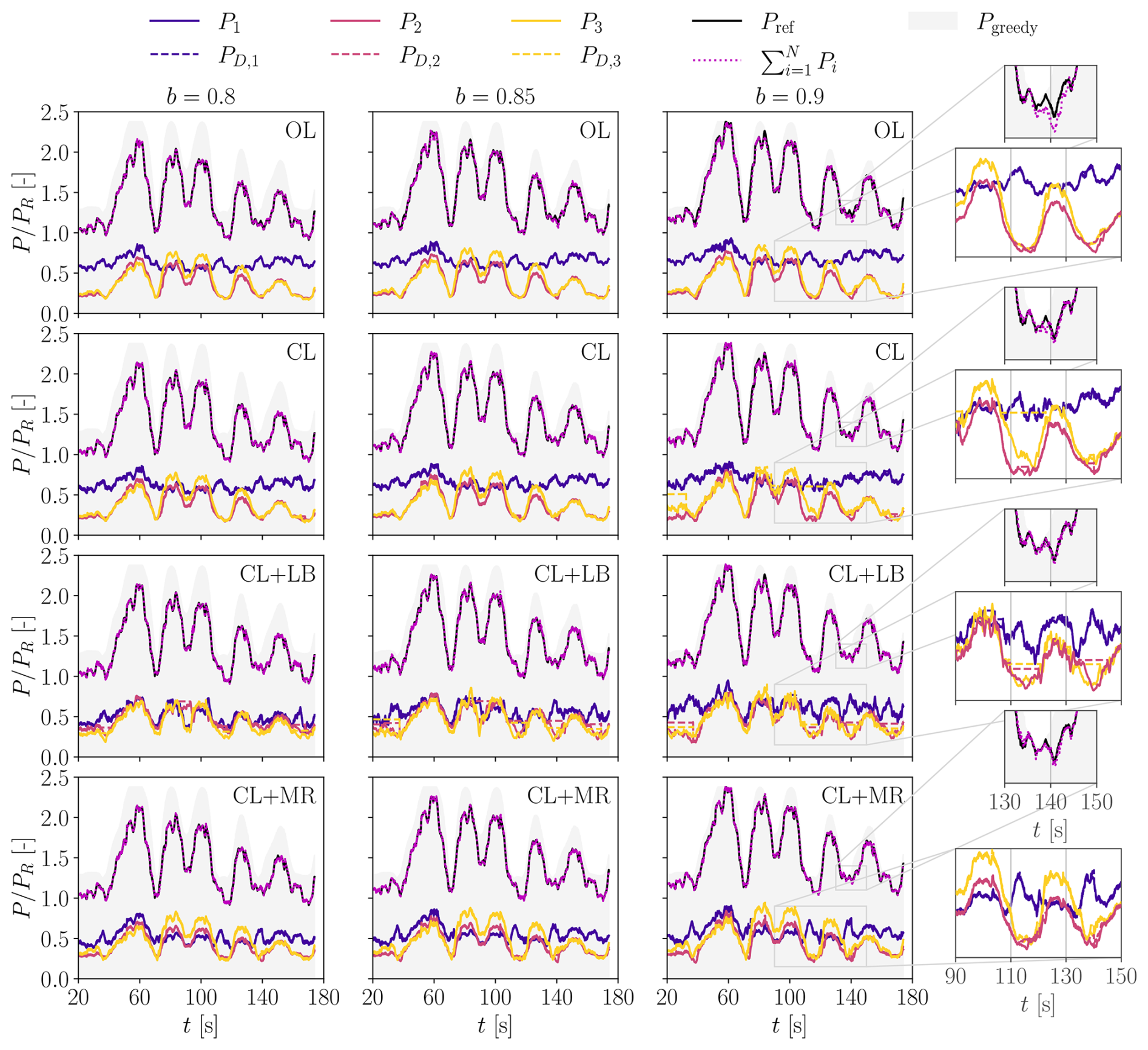
Figure 21 Time series of a power tracking experiment with dynamic wind direction variation, for the four APC algorithms and three power-demand levels b. The expected available wind farm power in greedy mode – based on the instantaneous wind direction – is shown in the background in gray.

From a first qualitative impression, all methods seem to follow the reference signal accurately. It is clear that OL and CL share the same power share set-points α_i, since P_D,1, P_D,2, and P_D,3 are similar. In CL, however, some saturations can be seen, for instance when t≈100 s and b=0.9. CL+LB presents a very different distribution of power shares, and it appears that the individual power outputs P_D,i of the three turbines are often similar, possibly to balance the loads in conditions of low wake impingement. The power share distribution of CL+MR resembles that of OL, although P_D,1 is generally lower and P_D,3 higher due to wake steering.

Overall, the plots clearly show that, as the power demand is increased, the power request P_ref approaches the greedy power, and more saturation events arise, as indicated by the flat lines of P_D,i in CL, CL+LB, and CL+MR.

In the zoomed windows of the plot, an example is highlighted where OL presents a significant deviation from P_ref at the wind farm level, because of a saturation of WT₂ lasting approximately 10 s. This same problem also occurs for CL. However, the wind farm tracking error is clearly reduced because WT₁ and WT₃ are able to compensate. Quite differently, CL+LB and CL+MR show excellent tracking performance in the same scenario. This similar performance is, however, achieved in different ways: in CL+LB, both WT₂ and WT₃ are saturated and therefore operate in greedy mode, while WT₁ is fully responsible for tracking P_ref. In CL+MR, no saturation events are visible, which indicates generally larger power reserves for all turbines.

To present a more complete picture of the performance of the various algorithms, Appendix D reports additional zoomed segments of the plots shown in Fig. 21.

6.1 Power tracking accuracy

The RMS of the tracking error is shown in Fig. 22.

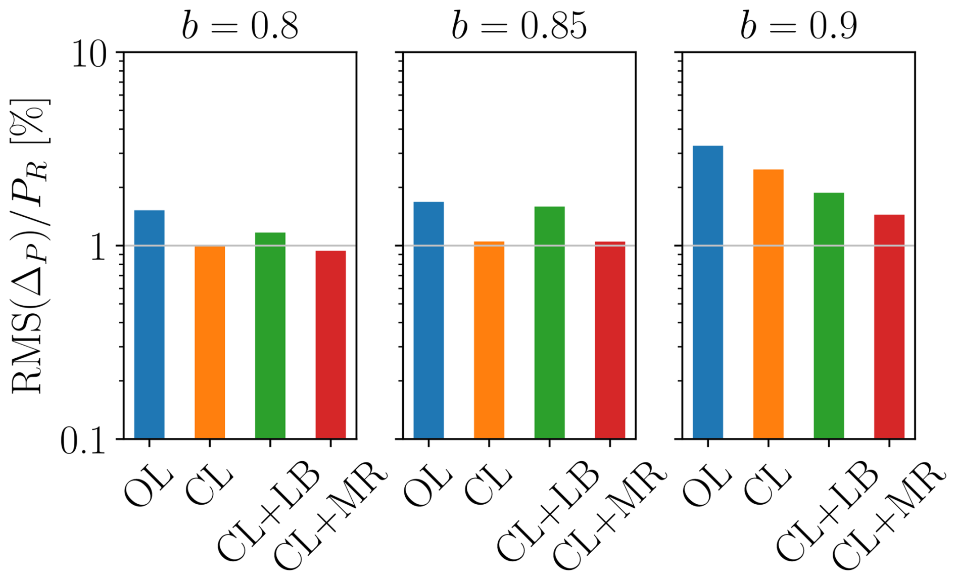
Figure 22 RMS of power tracking errors for the four APC algorithms and three power-demand levels b. Experiment with dynamic wind direction variations.

Consistently with the static wind direction results, OL shows the worst performance of all APC methods. At moderate power demands, for b≤0.85, CL and CL+MR exhibit the best performance. For b=0.9, CL+MR provides the lowest RMS Δ_P. The relative improvements achieved by CL+MR are less pronounced in the dynamic tests than in the static ones, as the effects of wake steering are less beneficial at large turntable misalignments where wake interactions are much reduced.

Figure 23 shows how the errors are distributed across the three turbines. It is important to mention that saturated turbines will display extreme error values Δ_P,i, although this does not necessarily imply a large wind farm tracking error Δ_P, since (except than for OL) non-saturated rotors can compensate for their error.

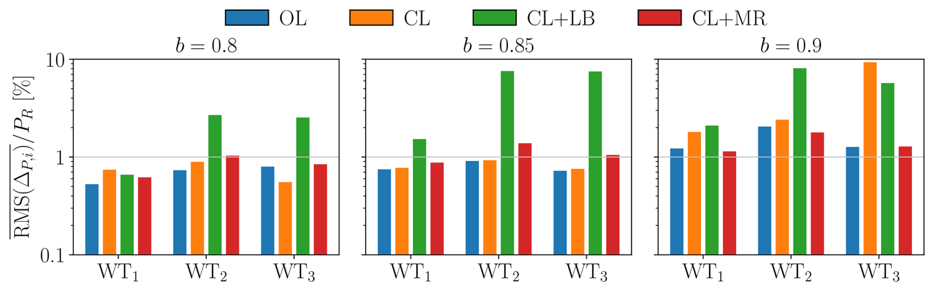
Figure 23 Local RMS of power tracking errors for the four APC algorithms and three power-demand levels b. Experiment with dynamic wind direction variations.

The figure shows relatively large tracking errors for OL, because of a lack of feedback capable of handling saturation conditions. Significant tracking errors can be observed for waked rotors in the case CL+LB, indicating persistent saturations, as seen in the zoomed regions of Fig. 21.

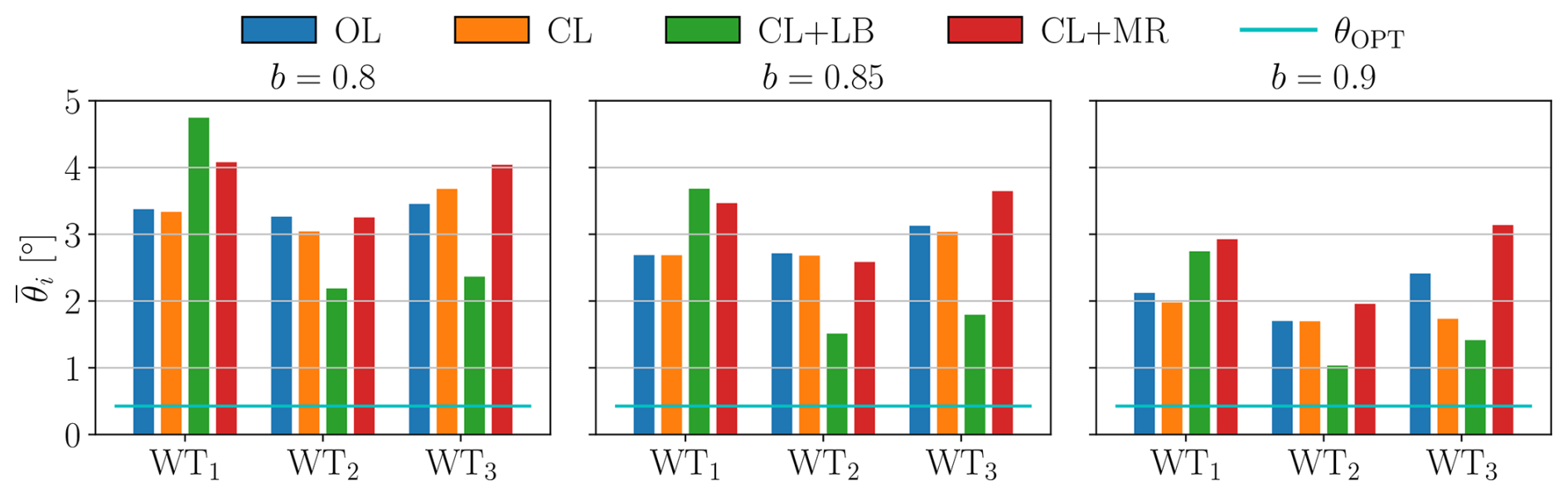
Figure 24 Mean collective blade pitch angle $\stackrel{\mathrm{‾}}{\mathit{\theta }}$ for the four APC algorithms and three power-demand levels b. Experiment with dynamic wind direction variations.

Figure 24 supports this analysis by presenting the mean collective blade pitch angles of the turbines during the experiment. As mentioned in the static direction study, ${\stackrel{\mathrm{‾}}{\mathit{\theta }}}_i$ can be seen as an indirect measure of the power reserve for the ith turbine.

Results show that CL+LB presents a significantly unbalanced power reserve distribution, shifted toward the upstream rotor, possibly as a result of the CLD loop. This is in agreement with the other quantities presented and discussed earlier in this section. As expected, CL+MR presents a rather large power reserve for all rotors, especially for WT₃, thanks to wake steering, but also for WT₁, which is remarkable since this upstream turbine is often misaligned.

6.2 Loads and fatigue

Figure 25 presents the mean load-balancing error for the dynamic turntable experiment.

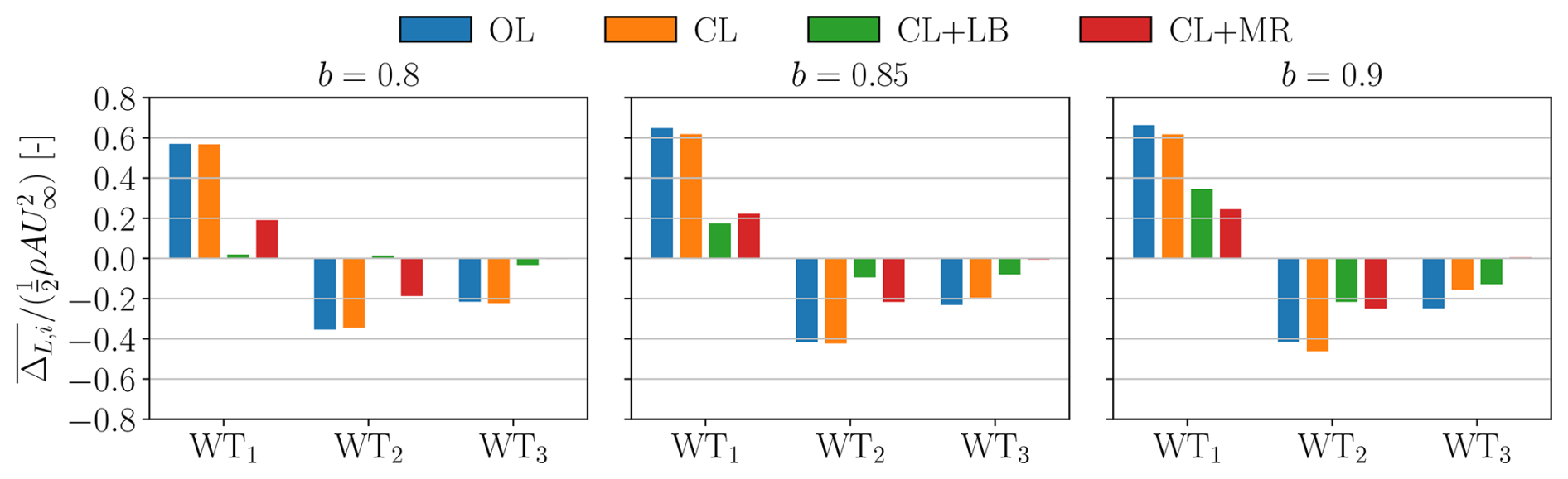
Figure 25 Mean local load-balancing error for tower-base fore-aft bending for the four APC algorithms and three power-demand levels b. The error is normalized by $\frac{\mathrm{1}}{\mathrm{2}}\mathit{\rho }{U}_{\mathrm{\infty }}^{\mathrm{2}}$. Positive values indicate loading above the wind farm average. Experiment with dynamic wind direction variations.

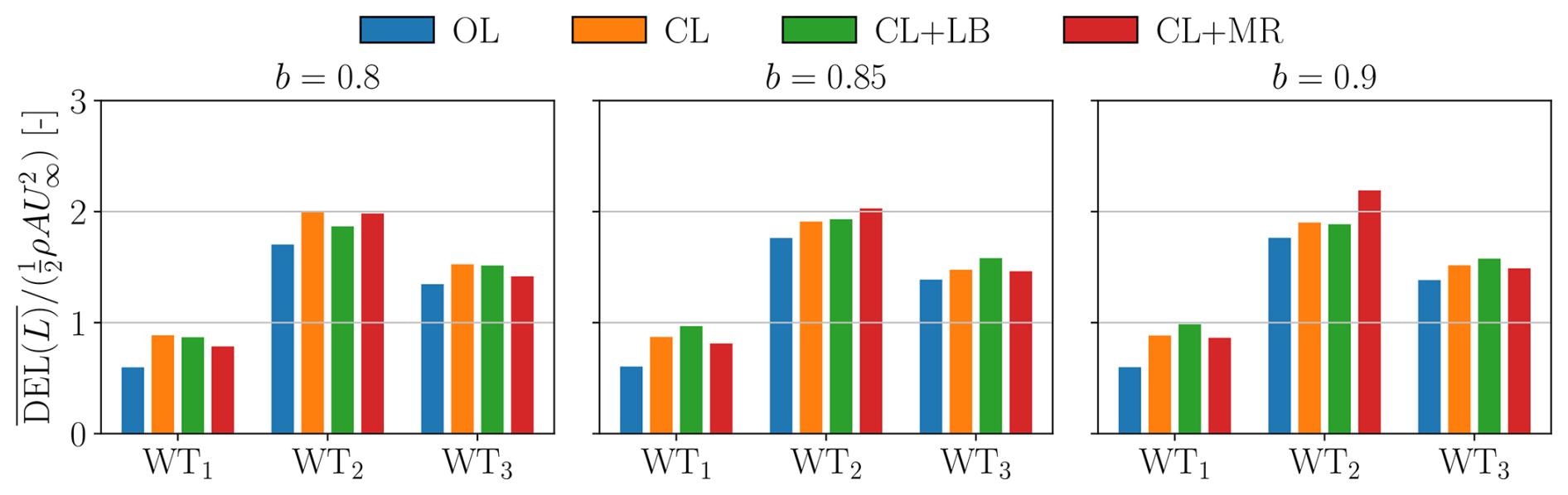
Figure 26 Tower-base fore-aft DELs for the four APC algorithms and three power-demand levels b. DELs are normalized by $\frac{\mathrm{1}}{\mathrm{2}}\mathit{\rho }{U}_{\mathrm{\infty }}^{\mathrm{2}}$. Experiment with dynamic wind direction variations.

For OL and CL, the front turbine WT₁ exhibits the highest loading, which progressively diminishes for rotors located further downstream. As seen already in the static cases, CL+LB effectively balances the loads. Its effectiveness is excellent at b=0.8 but – importantly – gradually deteriorates as b increases since more saturation events arise that modify the power share distribution to prioritize tracking accuracy. CL+MR displays the second-best performance for the lower b values but ultimately outperforms CL+LB for b=0.9. This shows the importance of controlling saturations and the limits of a purely load-balancing strategy.

Figure 26 reports the normalized tower-base fore-aft DELs.

These results generally indicate a higher fatigue for WT₂, followed by WT₃ and WT₁, which is the least-affected turbine. WT₂ is also the rotor that generally has the smallest power margin in the farm, as shown in Fig. 24. This result is consistent with the findings of Tamaro et al. (2025b), which showed that fatigue is driven by the low-frequency load cycles that occur because of saturation events. OL generally exhibits the lowest fatigue, due to the smoother control of the rotors. The proposed CL+MR method reduces $\stackrel{\mathrm{‾}}{\text{DEL}\left(L\right)}$ for WT₁ and WT₃ compared to other methods featuring a closed loop, while it increases it for WT₂, possibly due to a lower power margin deriving from the α_i and γ_i LUTs.

7 Conclusions

A maximum-reserve approach for robust wind farm power tracking that combines wake steering and induction control has been tested experimentally in a wind tunnel. The objective of the algorithm is to enhance power reserves across the wind farm to mitigate the effects of wind lulls, thereby generating a more accurate tracking of the desired power signal.

To support the experimental work, a steady-state model was developed, based on a modified version of FLORIS. This model accounts for the aerodynamic interactions resulting from simultaneous yaw misalignment and curtailed operation, as well as specific wind tunnel inflow characteristics and chord-based Reynolds number effects caused by the small scale of the turbines.

The experiments were conducted in a large boundary-layer wind tunnel using a small cluster of three scaled rotors with minimal blockage. The first set of experiments considered two wind farm layouts to replicate varying levels of wake impingement. A second unprecedented set of APC experiments involved dynamically varying the wind direction using a large turntable.

The maximum-reserve method was compared with three alternative APC algorithms sourced from the recent literature. All controllers were implemented on a dedicated cabinet, enabling real-time communication to and from the controllers running on the individual turbines. The performance of the various controllers was evaluated in terms of power tracking accuracy, power reserves, structural loads, and fatigue.

The main findings of this study are as follows:

• A steady-state analysis confirms that wake impingement reduces the power reserves of downstream rotors. The combined use of wake steering and induction control effectively enhances local power reserves, thereby improving overall power tracking accuracy.

• The treatment of saturation conditions significantly affects power tracking performance. The open-loop algorithm showed the poorest performance in most cases. However, introducing a simple feedback loop and a compensation strategy for saturated rotors led to substantial improvements.

• Results from the dynamic wind direction experiments corroborated the findings from the fixed-direction runs, highlighting the strong potential of wake control in APC applications.

• Dispatching power set-points to balance loads proved effective in reducing fatigue compared to both open-loop and closed-loop controllers with fixed set-points. However, load-balancing set-points may lead to localized saturation, particularly at high power-demand levels, which in turn negatively affects loading.

Future work may extend this study by investigating the role of curtailment strategies on power tracking performance. Another area of investigation that should be pursued is the direct inclusion of loads in the maximum-reserve formulation because, as seen here, the correct management of reserves can have major implications on loading.

Appendix A: Floris wake parameters

Tables A1–A3 present the values of the parameters of the wake deflection, turbulence, and wake deficit models, respectively.

Table A1 Values of the parameters of the deflection model (Bastankhah and Porté-Agel, 2014).

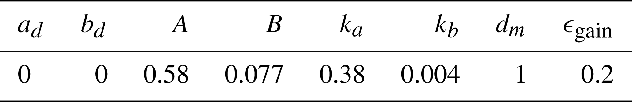
Table A2 Values of the parameters of the turbulence model (Crespo and Hernàndez, 1996).

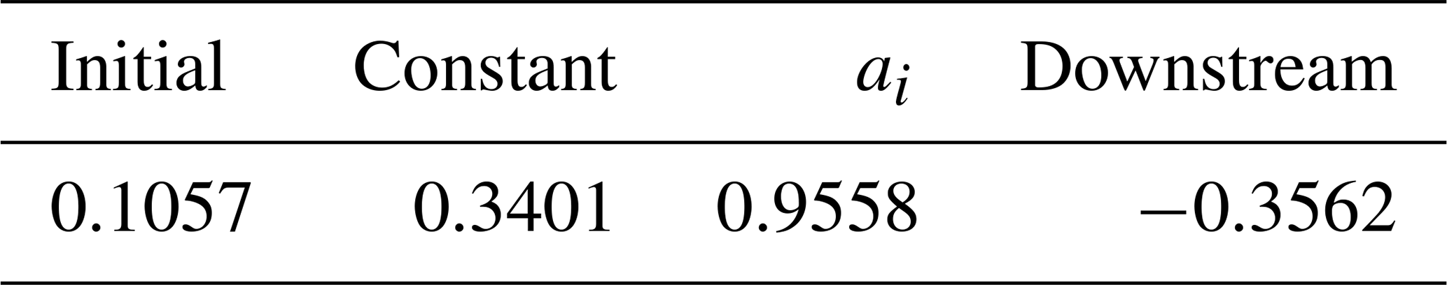
Table A3 Values of the parameters of the Gauss deficit model (Bastankhah and Porté-Agel, 2014).

Appendix B: Blade pitch actuator duty cycle

The actuator duty cycle (ADC) of blade pitch is shown for the static turntable experiments in Figs. B1 and B2 for ψ=2.8° and ψ=5.7°, respectively. ADC for the blade pitch angle θ is defined as (Bottasso et al., 2013)

$$\begin{array}{}\text{(B1)}& {\displaystyle }{\displaystyle }{\text{ADC}}_{\mathit{\theta }}={\displaystyle \frac{\mathrm{1}}{T}}\underset{\mathrm{0}}{\overset{T}{\int }}{\displaystyle \frac{\dot{\mathit{\theta }}\left(t\right)}{{\dot{\mathit{\theta }}}_{max}}}\mathrm{d}t,\end{array}$$

where $\dot{\mathit{\theta }}$ is the pitch rate.

Results appear to be strongly dependent on the power-demand level b. When b=0.8, waked turbines show a higher pitch activity than the upstream turbine WT₁. This condition persists for OL and CL+MR in most of the other b scenarios and for both wind directions ψ. For CL and CL+MR, on the contrary, for b=0.9, it is the front turbine WT₁ that displays the highest pitch activity, due to the need to compensate for saturation events occurring at the downstream waked turbines. It should also be noted that when a turbine saturates, its pitch lies at θ=θ_OPT until the saturation criteria are not met anymore, and this automatically reduces ADC.

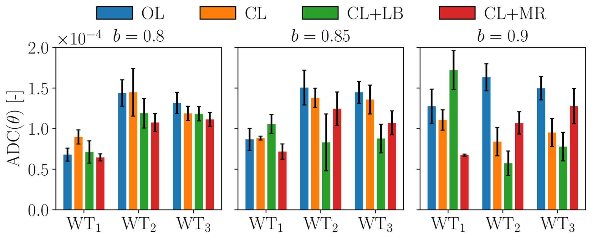
Figure B1 Blade pitch ADC for the static turntable experiment with wind direction ψ=2.8°, corresponding to 75 % rotor overlap. Whiskers indicate 95 % confidence intervals. Results are presented for three power-demand requests b.

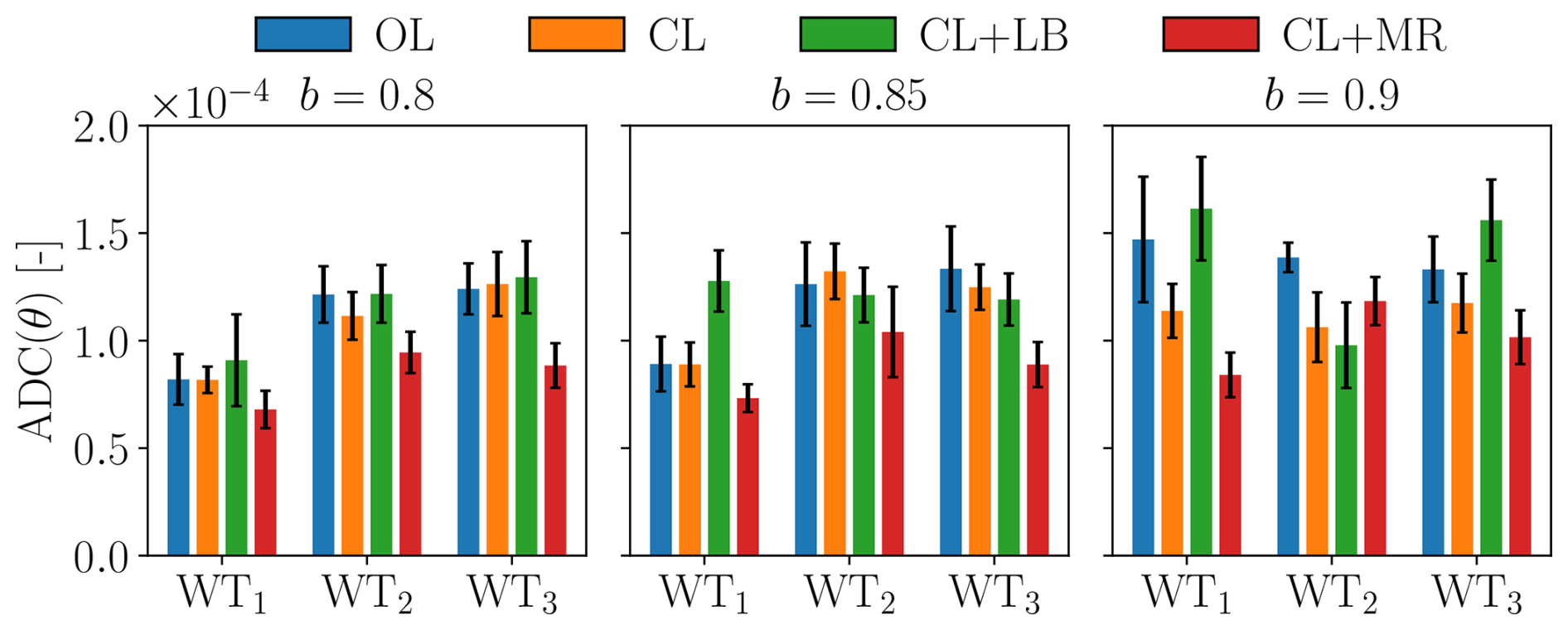
Figure B2 Blade pitch ADC for the static turntable experiment with wind direction ψ=5.7°, corresponding to 50 % rotor overlap. Whiskers indicate 95 % confidence intervals. Results are presented for three power-demand requests b.

Appendix C: Load-balancing error

For completeness, Fig. C1 reports the mean local load-balancing error for the case ψ=5.7° (50 % rotor overlap). The case ψ=5.7° (75 % rotor overlap) was shown earlier in Fig. 19.

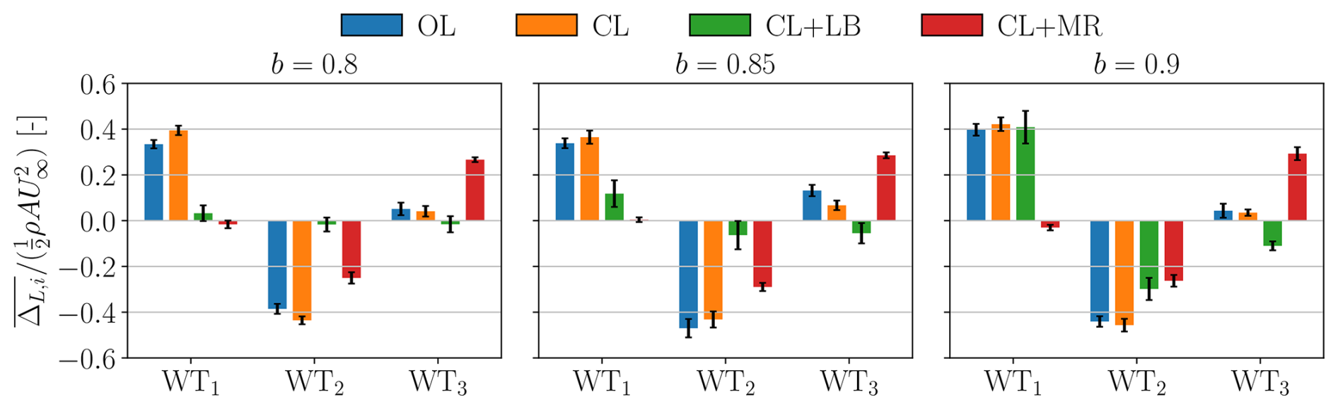
Figure C1 Mean local load-balancing error for the tower-base fore-aft bending moment for the static turntable experiment with wind direction ψ=5.7°, corresponding to 75 % rotor overlap. L is normalized with $\frac{\mathrm{1}}{\mathrm{2}}\mathit{\rho }{U}_{\mathrm{\infty }}^{\mathrm{2}}$. Positive values indicate loading above the wind farm average. Results are presented for three power-demand requests b.

Appendix D: Zoomed segments of Fig. 21 (power tracking time series under dynamic wind direction conditions)

This Appendix reports zoomed segments of the power tracking time series shown in Fig. 21, which were obtained under dynamic wind direction conditions.

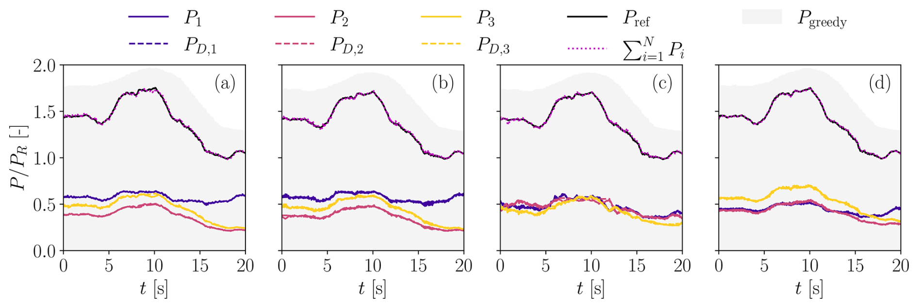
Figure D1 Enlarged segment of time series of a power tracking experiment with dynamic wind direction variation for a power-demand level b=0.8. The wind farm control strategies are OL (a), CL (b), CL+LB (c), and CL+MR (d). The expected available wind farm power in greedy mode – based on the instantaneous wind direction – is shown in the background in gray.

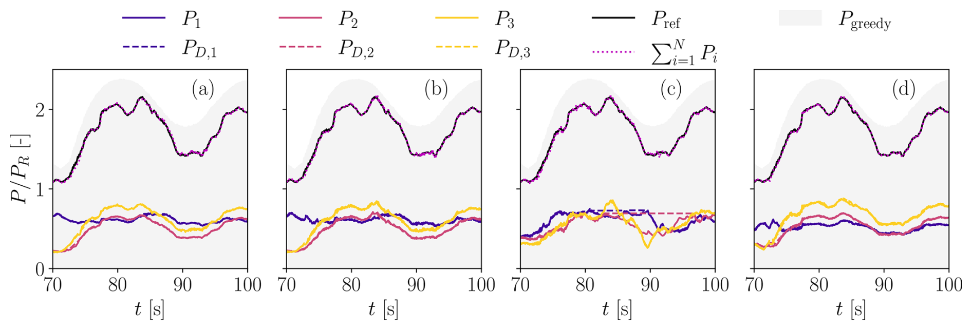
Figure D2 Enlarged segment of time series of a power tracking experiment with dynamic wind direction variation, for a power-demand level b=0.85. The wind farm control strategies are OL (a), CL (b), CL+LB (c), and CL+MR (d). The expected available wind farm power in greedy mode – based on the instantaneous wind direction – is shown in the background in gray.

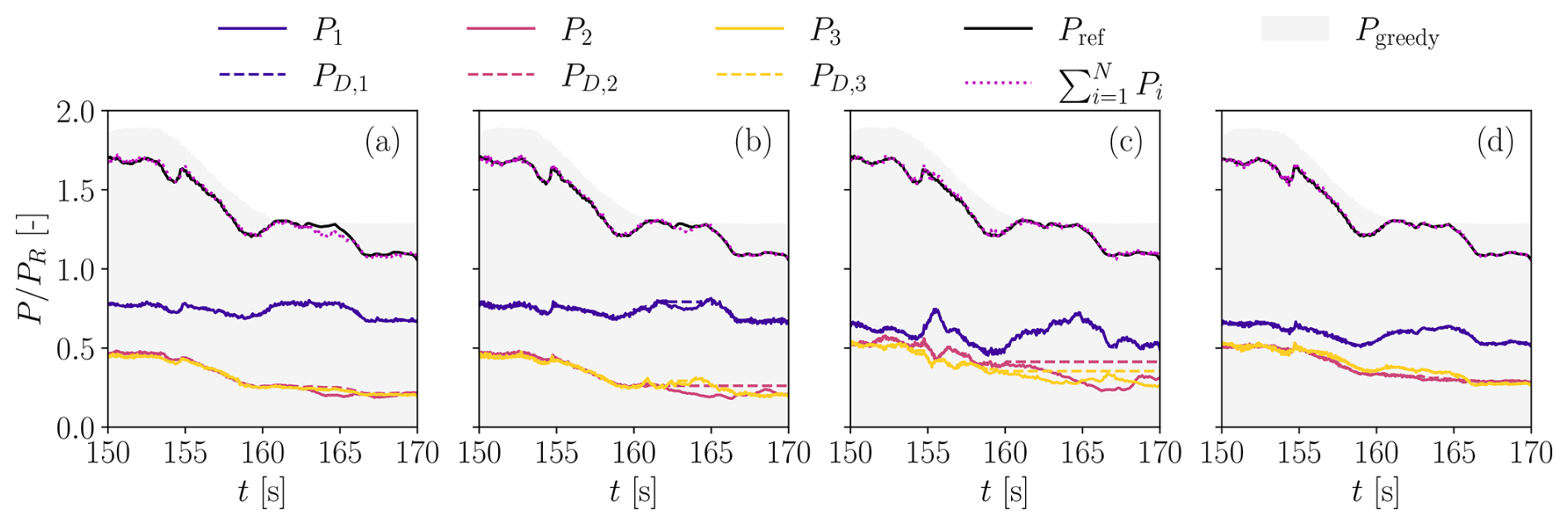
Figure D3 Enlarged segment of time series of a power tracking experiment with dynamic wind direction variation, for a power-demand level b=0.9. The wind farm control strategies are OL (a), CL (b), CL+LB (c), and CL+MR (d). The expected available wind farm power in greedy mode – based on the instantaneous wind direction – is shown in the background in gray.

Figure D1 presents the first 20 s of the experiment for a low average power-demand level b=0.8. The plots highlight the similar power share distributions of OL and CL. OL presents a slight deviation from P_ref at t=10 s, which is improved in CL thanks to the closed-loop correction that it implements. Figure D1c shows that the power share distribution is equal among the rotors for CL+LB. Although a saturation of WT₂ occurs at t=10 s, it does not affect the power tracking accuracy, because WT₁ and WT₃ adjust their power demand to compensate. Finally, Fig. D1d shows that the power share distribution generated by CL+MR is significantly different from the other cases, with WT₃ producing the most power as a result of the wake steering performed by the upstream turbines. The power outputs of the turbines also appear to be much smoother than in the other cases.

Next, Fig. D2 presents 8 s from experiments conducted with a larger average power-demand level equal to b=0.85. Figure D2a clearly shows the difficulty of the OL controller in tracking P_ref at t=60 s. In particular, P₁ exhibits significant deviations from P_D,1. The figure shows also that CL and CL+MR are able to improve the power tracking accuracy; however, even in these cases, WT₁ struggles to follow its demand, leading to saturations – for instance at t=62 s. In CL+LB, the load-balancing loop tends to equalize the power shares, but this results in a reduced power reserve for WT₂, which in fact saturates at t=62 s.

Finally, Fig. D3 focuses on 20 s toward the end of the experiments for a high average power-demand level b=0.9. The plots clearly show that both OL and CL exhibit critical tracking errors at t=164 s, with WT₂ being responsible for the error in both cases. In CL, this leads to its saturation. It is also clearly visible that, as P_D,1 is increased due to the saturation of WT₂, WT₁ saturates as well. Figure D3c shows that the load-balancing algorithm attempts to increase the power share of WT₂ and WT₃ at t=155 s. However, this is incompatible with their local power reserves and results in the saturation of both rotors for t>160 s. Nevertheless, the local power tracking errors of WT₂ and WT₃ are redistributed to WT₁, which is able to ensure good tracking of P_ref. For CL+MR, the turbine power outputs are smoother and free from saturations.

Appendix E: Nomenclature

A	Ambient conditions
b	Shift of normalized power-demand signal (i.e., average power-demand level)
CP	Power coefficient
CT	Thrust coefficient
c	Amplitude of normalized power-demand signal
D	Rotor diameter
KI	Control gain (integral)
KP	Control gain (proportional)
L	Tower-base fore-aft bending moment
m	Power reserve
N	Total number of wind turbines
$n_k^{\text{AGC}}$	Normalized power-demand signal
P	Wind turbine power
PD	Wind turbine power demand
PR	Rated power
Pref	Reference power signal
$P_{\text{ref}}^{\text{PI}}$	Closed-loop APC control output
R	Rotor radius
S	Number of saturated rotors
t	Time
U	Rotor-equivalent wind speed
U∞	Freestream wind speed measured at hub height
u	Control inputs
α	Power share set-point
γ	Misalignment angle
ΔL	Load-balancing error
ΔP	Power tracking error
ϵ	Auxiliary power scaling factor
ηP	Power loss factor
θ	Blade pitch angle
λ	Tip speed ratio
ρ	Air density
τ	Time instant index
ψ	Wind direction
Ω	Rotor angular speed
ΩR	Rated rotor angular speed
AGC	Automatic generation control
APC	Active power control
CL	Closed loop
CLD	Coordinated load distribution
CL+LB	Closed loop with load balancing
CL+MR	Closed loop with maximum reserve
DEL	Damage equivalent load
LUT	Lookup table
FLORIS	FLOw Redirection and Induction in Steady State
OL	Open loop
PI	Proportional – integral
RMS	Root mean square
TI	Turbulence intensity
TSO	Transmission system operator
WF	Wind farm
WT	Wind turbine