Wind field estimation for lidar-assisted control: a comparison of proper orthogonal decomposition and interpolation techniques

This study presents and evaluates three wind field reconstruction methods for real-time inflow characterization, with potential applications in lidar-assisted wind turbine control. The first method applies a least-squares fit of proper orthogonal decomposition (POD) modes to lidar measurements (POD-LSQ). The second uses inverse distance weighting (IDW) interpolation across the rotor plane. The third, POD-IDW, applies the POD-LSQ fit to the interpolated field. The methods are tested under semi-realistic conditions derived from large-eddy simulations (LESs), using a hub-mounted lidar sensor implemented in HAWC2 on the DTU 10 MW reference turbine. Measurements are extracted under varying inflow conditions. A rotor-effective wind speed estimate, combined with the known vertical shear profile from LES, serves as the baseline for comparison. Reconstruction performance is quantified using a global mean absolute error, evaluated across combinations of scan count, POD mode number, and lidar beam angle. Optimal parameters are selected based on the minimum error. To assess physical accuracy, reconstructions are compared against true wind speeds, evaluating the effects of probe volume averaging, multi-distance measurement selection, cross-contamination, and other sources of error. For optimal inputs, POD-IDW achieves the highest accuracy, reducing error by 45.5 % compared with the baseline estimation, at 5.4 times the computational cost. IDW performs similarly (44.9 %) with optimal inputs, while POD-LSQ achieves a 39.4 % reduction with minimal overhead (7 %). Spectral analysis shows that volume averaging and scanning strategies introduce low-pass filtering that attenuates high-frequency turbulence, while preserving low-frequency content more accurately than the baseline. Reconstruction quality strongly depends on the number and spatial distribution of lidar measurements and the number of retained POD modes. Although demonstrated under idealized conditions, the methods show strong potential for real-time applications. Future work should integrate these reconstructions with flow-aware controllers to evaluate fatigue load reduction, particularly at tower level.

1 Introduction

The upscaling of wind turbines has led to increasingly large and flexible rotors. While larger rotors average out small-scale fluctuations, they also increase sensitivity to spatio-temporal wind variability, which impacts both power production and structural loading (Angelou and Sjöholm, 2022). To mitigate these effects, advanced control strategies are needed to enhance performance while minimizing fatigue and extreme loads (Dong et al., 2021; Angelou and Sjöholm, 2022; Russell et al., 2024).

Lidar-assisted control (LAC) has emerged as a promising approach to reduce fatigue loads (Bossanyi et al., 2012; Guo et al., 2023; Fu et al., 2023; Russell et al., 2024), extreme loads (Schlipf and Kühn, 2008), and the levelized cost of energy (Scholbrock et al., 2016; Simley et al., 2018). Conventional LAC systems use nacelle-mounted lidars, which measure upstream wind via Doppler sensing and enable feedforward control by anticipating turbulence (Bossanyi et al., 2012; Schlipf et al., 2015; Simley et al., 2018). However, nacelle-mounted lidars performance is hindered by blade blockage, causing data loss and increased uncertainty in wind field estimation (Schlipf et al., 2018; Angelou and Sjöholm, 2022). Mounting the lidar on the hub or spinner (hereafter hub lidar) mitigates blockage and improves scan availability.

While hub mounting addresses the geometric source of data loss, data availability and reconstruction fidelity are also shaped by the lidar measurement principle itself. Continuous-wave (CW) lidars measure wind speed at a single-focus distance through a range-weighted probe volume, whereas pulsed lidars use range gating to retrieve velocities at multiple distances along the line of sight (LOS) (Peña et al., 2015); however, this broader spatial coverage is typically achieved at the expense of longer effective sampling times than CW systems (Letizia et al., 2023). Building upon the blockage mitigation provided by hub mounting, a pulsed hub lidar combines multi-range, longer-range measurements with improved scan availability, thereby providing spatially distributed inflow observations that are well suited for wind field reconstruction and subsequent LAC feedforward control, depending on appropriate lidar configuration selection.

Among LAC strategies, feedforward collective pitch control is the most established. It adjusts all blades simultaneously by using REWS estimated as the averaged wind velocities measured by the lidar and projected into the longitudinal direction (Held and Mann, 2019), improving rotor speed regulation and reducing loads (Dunne et al., 2011; Canet et al., 2021; Fu et al., 2023). However, reliance on spatially averaged REWS becomes less valid as rotor size increases.

To address this, feedforward individual pitch control adjusts each blade independently in response to localized wind. Approaches include combining REWS with horizontal and vertical shear profiles (Schlipf et al., 2010; Dunne et al., 2012) or measuring blade-level wind speeds at fixed radial and azimuthal positions (Dunne et al., 2012; Russell et al., 2024). Despite their benefits, these methods rely on simplified inflow assumptions and do not resolve spatio-temporal structures, which become increasingly inadequate for large rotor diameters. Thus, there is a critical need for real-time, high-fidelity wind field reconstruction algorithms capable of resolving the spatial and temporal structures of the incoming wind, enabling more advanced LAC strategies and improved load mitigation across both tower and blade components.

High-fidelity reconstruction methods are therefore needed to capture the full wind field dynamics. Spectral techniques (Dimitrov and Natarajan, 2016; Rinker, 2022; Fu et al., 2022; Guo et al., 2022), CFD-based optimization (Bauweraerts and Meyers, 2021), and Bayesian estimation (Bauweraerts and Meyers, 2020) exist but are computationally intensive and not suited for real-time applications. Physics-informed machine learning approaches show promise for fast inflow reconstruction (Zhang and Zhao, 2021a, b) but lack demonstrated scalability for utility-scale turbines.

Proper orthogonal decomposition (POD) offers a computationally efficient model reduction technique by decomposing velocity fields into spatial modes and time-dependent coefficients that capture the flow's temporal evolution. It has been used in wind energy to study turbine wakes for individual flow cases (VerHulst and Meneveau, 2014; Newman et al., 2014; Andersen et al., 2017; De Cillis et al., 2020). While early POD applications lacked predictive generality (Meneveau, 2019), Andersen and Murcia Leon (2022) introduced a global POD basis by combining multiple flow cases, allowing the basis to span a broader parameter space and enabling consistent physical interpretation across different flow conditions. More recently, Céspedes Moreno et al. (2025) evaluated the performance of a global basis in reconstructing wake aerodynamics, showing that the reconstruction error decreases and converges as more cases are included in the dataset.

Focusing now on the use of lidar measurements in combination with POD, recent studies have explored both wake characterization and inflow reconstruction. In the context of wakes, Hamilton et al. (2025) applied POD to horizontal scans from nacelle-mounted lidars to identify coherent turbulent structures experienced by a turbine operating in the wake of an upstream rotor. For inflow reconstruction, Sekar et al. (2022); Kidambi Sekar et al. (2022) combined SpinnerLidar measurements with POD to estimate the incoming turbulent wind field. However, their approach relies on a complex and non-commercial lidar system (Mikkelsen et al., 2013; Herges et al., 2017), and it requires prior knowledge of the inflow, limiting its predictive capability. To address these limitations, Soto Sagredo et al. (2024a) proposed a least-squares fit of POD (POD-LSQ) method using hub-lidar data to estimate modal amplitudes in real time without requiring prior flow information. While promising, this approach was developed using idealized Mann-generated turbulence (Mann, 1998), and its robustness under realistic inflow conditions remains to be demonstrated.

Interpolation offers another approach for inflow reconstruction. Techniques such as kriging, inverse distance weighting (IDW), and cokriging are widely used in meteorology to estimate wind from sparse data (Luo et al., 2007; Joyner et al., 2015; Friedland et al., 2016). Similar methods have been applied to lidar-based wind field reconstruction (Chu et al., 2021; Bao et al., 2022), though they struggle to resolve unsteady 3D flow structures due to limited coverage and assumptions. In a related context, Beck and Kühn (2019) developed a space–time conversion method for planar long-range Doppler lidar measurements, employing spatial interpolation as part of a temporal up-sampling framework for wind turbine wake fields; while their focus is on correcting scan-inherent time shifts rather than inflow reconstruction, the work illustrates the broader role that interpolation schemes play in recovering wind field information from spatially and temporally sparse lidar data. Particularly, IDW is a widely used interpolation technique in geosciences, environmental science, and spatial data analysis (Bokati et al., 2022) and was also used by Soto Sagredo et al. (2024b) to reconstruct rotor plane wind fields using hub-lidar data. While promising for real-time use, that study focused on idealized conditions and a single wind speed.

This study addresses the need for robust, real-time wind field reconstruction under varying inflow conditions. We evaluate three techniques: POD-LSQ, IDW, and a hybrid POD-IDW approach, comparing them against a REWS-based baseline that includes the vertical shear profile. Using LES-generated inflow and a numerical six-beam pulsed hub lidar, we assess reconstruction accuracy and sensitivity to different input parameters across methods and inflow conditions. In particular, POD-LSQ shows promise for LAC due to its computational efficiency and spatial fidelity.

The paper is structured as follows. Section 2 describes the methodology, including LES inflow, lidar setup, and reconstruction methods. Section 3 evaluates the performance of each method across varying inflow conditions, analyzing their sensitivity to input parameters and measurement uncertainty to identify the optimal parameter combinations for each reconstruction approach. Section 4 discusses implications and limitations, while Sect. 5 concludes the paper and outlines future work.

2 Methodology

To evaluate the wind field estimation techniques, synthetic lidar data are generated using high-fidelity inflow conditions from LES and a numerical hub-lidar sensor implemented on the DTU 10 MW reference wind turbine (RWT) model (Bak et al., 2013) in HAWC2 v13.1 (DTU Wind Energy, 2024), which includes a flexible tower and a 5° tilt. The methodology is first summarized in the following paragraphs before being described in detail in the subsequent subsections.

An overview of the wind field reconstruction concept using pulsed hub-lidar technology is shown in Fig. 1. The multi-distance projected LOS velocities captured by the hub lidar are mapped onto a reconstruction plane, where an estimation method reconstructs the spatio-temporal wind field. This high-resolution inflow can potentially support advanced control strategies by enabling real-time adaptation to turbulent structures and improving load mitigation.

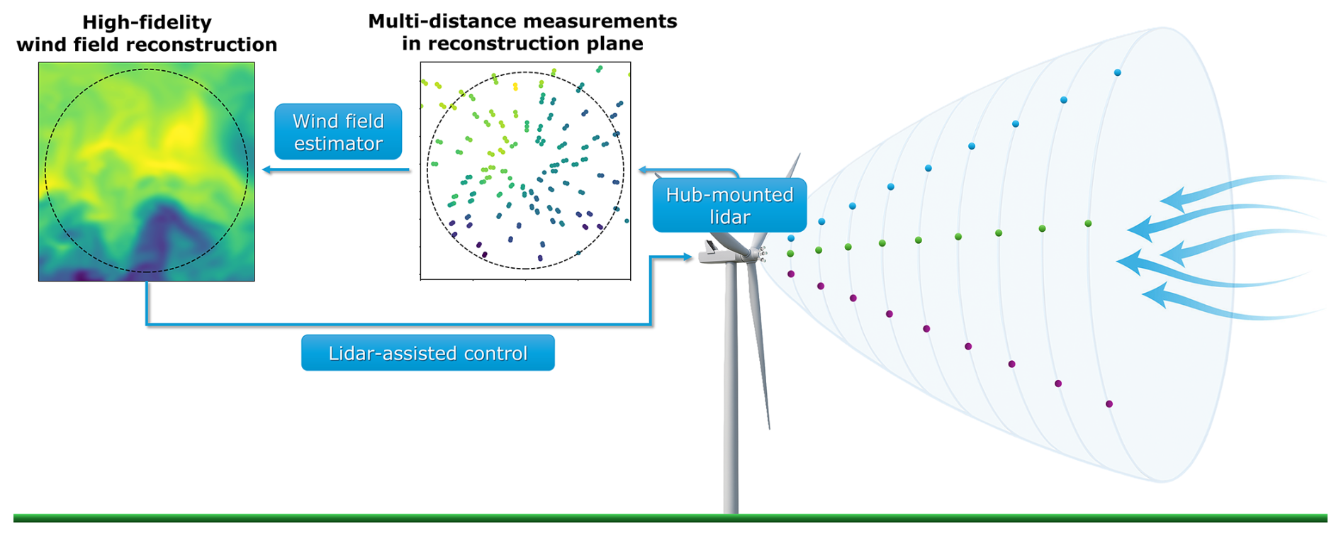
Figure 1 Schematic overview of the wind field reconstruction approach used in this study, using pulsed hub-lidar measurements for LAC.

Figure 2 outlines the numerical framework used to assess each method's accuracy. The primary goal is to quantify reconstruction error and analyze sensitivity to key input parameters: the lidar beam half-cone angle (θ), the number of scans (n_scan), the number of POD modes used for truncation (K), and the influence of measurement uncertainty.

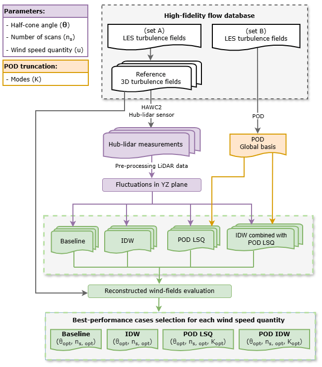
Figure 2 Numerical framework for wind field reconstruction evaluation using synthetic lidar measurements and four reconstruction techniques.

The process begins with a turbulence database derived from LES inflow fields, divided into two subsets: set A is used to extract hub-lidar measurements in HAWC2, serving as the reference dataset, while set B is used to construct the global POD basis. After preprocessing, the lidar data are mapped onto the reconstruction plane and decomposed into wind fluctuations in the YZ plane, which are then used as inputs to the reconstruction methods. The reconstructed fields are compared against the reference fields to compute the reconstruction error, where the best-performing cases across multiple inflow conditions are identified by selecting the parameter combinations that yield the lowest error. This systematic framework enables a consistent evaluation of each method and supports the identification of robust configurations suitable for real-time wind field reconstruction.

2.1 LES precursor

The LES data used in this study originate from precursor simulations by Andersen and Murcia Leon (2022).

The precursor simulates a neutral atmospheric boundary layer driven by a steady pressure gradient over flat terrain. It is performed using the EllipSys3D flow solver (Michelsen, 1992, 1994; Sørensen, 1995), which solves the Navier–Stokes equations in general curvilinear coordinates using a finite-volume method on a block-structured and collocated grid.

The computational domain spans $\mathrm{2880}\mathrm{m}\times \mathrm{1440}\mathrm{m}\times \mathrm{700.8}\mathrm{m}$, discretized into $\mathrm{576}\times \mathrm{288}\times \mathrm{320}$ cells, with uniform grid spacing of 5 m in the longitudinal and lateral directions and 2.19 m vertically. To avoid spanwise locking of turbulent structures, a lateral shift is applied to the periodic boundaries in the longitudinal direction, following Munters et al. (2016). The simulation assumes a surface roughness of $z_{\mathrm{0}}^{\text{org}}=\mathrm{0.05}\mathrm{m}$ and a friction velocity of $u_{*}^{\text{org}}=\mathrm{0.4545}\mathrm{m}{\mathrm{s}}^{-\mathrm{1}}$. It runs for 82 600 s (approximately 22.94 h) to ensure statistical convergence before collecting 28 800 s of inflow data.

As described by Castro (2007), neutral atmospheric boundary flows can be rescaled to generate multiple inflow conditions. We apply this rescaling following Troldborg et al. (2022):

$$\begin{array}{}\text{(1)}& {\displaystyle }{\displaystyle }{u}^{\text{new}}=u_{*}^{\text{new}}\left({\displaystyle \frac{u^{\text{org}}}{u_{*}^{\text{org}}}}+{\displaystyle \frac{\mathrm{1}}{\mathit{\kappa }}}\ln {\displaystyle \frac{z_{\mathrm{0}}^{\text{org}}}{z_{\mathrm{0}}^{\text{new}}}}\right),\end{array}$$

where κ=0.41 is the von Kármán constant, and the superscript “new” refers to the inflow condition to be generated, where $u^{\text{new}}\in [\mathrm{8.0},\mathrm{12.0},\mathrm{15.0},\mathrm{18.0}]\mathrm{m}{\mathrm{s}}^{-\mathrm{1}}$, obtaining four inflow wind speeds. All inflows have an average TI of approximately 11 %.

2.2 LES datasets

The LES datasets (sets A and B) are taken from two different locations within the LES domain and have distinct spatial dimensions in the lateral and vertical directions. Set A consists of $\mathrm{28}\mathrm{800}\times \mathrm{1}\times \mathrm{61}\times \mathrm{138}$ grid points ($t\times x\times y\times z$), while set B includes $\mathrm{28}\mathrm{800}\times \mathrm{1}\times \mathrm{39}\times \mathrm{91}$ grid points. Both datasets cover a 4 h period at a temporal resolution of d_t=0.5 s, with spatial resolutions of 5 m in the lateral (y) direction and 2.19 m in the vertical (z) direction. An illustration of the locations in the LES domains is given in Fig. A in the Appendix for clarity. For each inflow wind speed, the three turbulent velocity components (u, v, w) are extracted and rescaled following the method described in Sect. 2.1.

To ensure that the global POD basis characterizes the coherent turbulent structures over the rotor area, the spatial domain of set B is reduced and centered accordingly, spanning 190.3 m×197.1 m (y×z). In contrast, set A retains a larger spatial extent of 300.5 m×300.0 m (y×z), providing sufficient coverage for aeroelastic simulation and lidar probe volume modeling.

From set A, 16 non-overlapping 900 s segments are extracted to generate 16 independent 3D turbulent inflow fields. These are transformed into spatial boxes under Taylor's frozen turbulence hypothesis (Taylor, 1938), which assumes that turbulent structures are convected downstream at a constant advection velocity ${\overline{U}}_{\mathrm{o}}$ – the average wind speed at hub height – without evolving over time. Under this transformation, the time and longitudinal directions are combined to define the longitudinal coordinate x, with a spatial resolution given by

$${\displaystyle }{d}_x={\displaystyle \frac{{\overline{U}}_{\mathrm{o}}{T}_{\text{sim}}}{N_x}},\text{ where }{N}_x={\displaystyle \frac{T_{\text{sim}}}{d_{\mathrm{t}}}}=\mathrm{1800},T_{\text{sim}}=\mathrm{900}\mathrm{s}.$$

The resulting reference turbulence boxes have dimensions of $\mathrm{1800}\times \mathrm{61}\times \mathrm{138}$ grid points ($x\times y\times z$), enabling accurate 15 min HAWC2 simulations and ensuring full inclusion of lidar probe volume effects.

To account for HAWC2's transient effects, lidar initialization, and boundary effects, the first 250 s and the last 50 s of the simulation are discarded – beyond the conventional 100 s warm-up typically used in HAWC2 – yielding the final reconstructed wind fields of 600 s, with dimensions of $\mathrm{1200}\times \mathrm{39}\times \mathrm{91}$ grid points ($t\times y\times z$), with a time step d_t=0.5 s.

2.3 Proper orthogonal decomposition and global basis

POD decomposes turbulent flow into orthogonal spatial modes that optimally capture the variance of the fluctuations (Lumley, 1967; Berkooz et al., 1993). Typically, POD is applied to a single flow case, yielding an orthogonal basis optimized for that specific dataset.

To enable generalization across different flow conditions, Andersen and Murcia Leon (2022) utilized a “global” POD basis, which is derived by combining multiple cases, providing a more general representation across a broader parameter space. As the global POD modes are derived from multiple flow conditions, they are not optimized for any single case but instead capture generalized flow structures across the parameter space. However, as shown by Céspedes Moreno et al. (2025), the global basis is still very effective, and the suboptimality of a global basis compared to a “local” basis is at least an order of magnitude smaller than the truncation error.

To compute the basis, we first calculate the fluctuating component of the longitudinal velocity field by subtracting the temporal mean, $\overline{U}(y,z)$, from the full velocity field: ${\mathit{U}}^{\prime }(y,z,t)=\mathit{U}(y,z,t)-\overline{\mathit{U}}(y,z)$. These fluctuations are then reshaped into column vectors over N_t time steps for each of N_c flow cases, forming the matrix $\mathbf{M}=[{\mathit{U}}_{\mathrm{1},\mathrm{1}}^{\prime },\mathrm{\dots },{\mathit{U}}_{\mathrm{1},N_{\mathrm{t}}}^{\prime },\mathrm{\dots },{\mathit{U}}_{N_{\mathrm{c}},\mathrm{1}}^{\prime },\mathrm{\dots },{\mathit{U}}_{N_{\mathrm{c}},N_{\mathrm{t}}}^{\prime }]$, which is used to compute the POD modes using the randomized singular value decomposition (SVD) following the method of Halko et al. (2011).

The decomposition yields a set of orthonormal spatial modes $\mathbf{G}=[{\mathit{g}}_{\mathrm{1}},\mathrm{\dots },{\mathit{g}}_{N_{\mathrm{t}}-\mathrm{1}}]$. A visualization of the first 10 global POD modes is provided in Appendix B.

The corresponding modal time series are obtained by projecting the fluctuating flow onto the spatial POD modes using an inner product ${\mathit{\varphi }}_i\left(t\right)=〈{\mathit{U}}^{\prime }\left(t\right),{\mathit{g}}_i〉$.

A reduced-order approximation of the flow field can then be constructed as

$$\begin{array}{}\text{(2)}& {\displaystyle }{\displaystyle }\mathit{U}(y,z,t)=\sum _{i=\mathrm{1}}^K{\mathit{g}}_i(y,z){\mathit{\varphi }}_i\left(t\right)+\overline{U}(y,z),\end{array}$$

where $K<N_{\mathrm{t}}-\mathrm{1}$ is the number of retained modes, and ϕ_i(t) is the modal time coefficient. This approach provides a low-dimensional representation of the flow, retaining dominant coherent structures while reducing computational complexity.

Although accurate representation of the flow physics in POD requires all three velocity components ($u,v,w$) (Iqbal and Thomas, 2007), in this study we only extract the global POD modes using the longitudinal component (u) from the LES dataset set B (see Sect. 2.2). This choice reflects the focus on reconstructing the longitudinal wind speed, which is the primary quantity of interest for LAC applications. The simplification is motivated by both methodological and practical considerations. First, u component fluctuations dominate turbine loads (Dimitrov et al., 2018), whereas lateral (v) and vertical (w) components have a negligible impact (Dimitrov and Natarajan, 2016). Additionally, only the longitudinal u component can be estimated from the LOS. This limitation arises because the lidar does not measure the full 3D velocity vector; instead, it senses only the component projected along the beam direction (the “cyclops dilemma”) (Raach et al., 2014). Recovering individual velocity components from LOS measurements therefore requires additional assumptions. One option is to combine multiple beams under an assumption of local flow homogeneity (Sathe et al., 2015), which enables estimation of multiple velocity components (e.g., u, v, and/or w) but relies on limited spatial variability across the rotor. A second approach is to assume a known wind direction (e.g., align with the u component) and neglect the lateral and vertical components (Letizia et al., 2023). Because this study aims to resolve wind speed variations across the full rotor plane, we adopt the latter assumption and thus estimate only the longitudinal component u from the LOS measurements.

To avoid data leakage and promote generalization, the POD basis is computed from LES domains that are spatially offset from the reconstruction region (Appendix A).

2.4 Numerical lidar sensor

A numerical model of a hub-mounted pulsed lidar sensor is available in HAWC2 v13.1 (Soto Sagredo et al., 2023) to simulate realistic LOS wind measurements based on user-defined parameters for a single-beam lidar. This section outlines the sensor used in this study, including lidar parameters, coordinate system, and estimation of longitudinal wind speed.

The hub lidar consists of a pulsed single-beam sensor installed on the spinner and constrained to the wind turbine model, meaning that the lidar beams moves with the turbine structure and is affected by tower motion, including yaw, pitch, roll, and structural vibrations. As the spinner rotates, the beam sweeps the rotor area, measuring LOS wind speeds by projecting the local u, v, and w components onto the LOS direction (Fig. 1). Tower motion together with rotor rotation influences the measurements by introducing a relative-velocity contribution to the measured wind speed. However, in the current HAWC2 hub-lidar sensor implementation, rotor rotation does not introduce an additional translational velocity component into the measured wind speed. Motion-induced fluctuations are therefore dominated by tower motion and can be mitigated using frequency-domain filtering, which preserves the integrity of the estimated wind field without introducing bias (Gräfe et al., 2023). In practical deployments, such pre-processing should be applied before reconstructed inflow fields are used for load assessment or LAC because uncorrected motion artifacts can excite structural dynamics; inflate fatigue loads; and, in control applications, provoke undesirable actuator responses (Schlipf, 2016). Nevertheless, no motion correction or filtering has been applied in the present analysis because the study focuses on inflow reconstruction accuracy under multiple uncertainty sources.

Probe volume effects are simulated by HAWC2 using the weighting function and system parameters described in Meyer Forsting et al. (2017) for pulsed lidar systems. HAWC2 provides the following as outputs: (i) the probe-volume-averaged LOS velocity V_{LOS, wgh}; (ii) the nominal LOS velocity V_{LOS, nom}, without volume averaging; and (iii) the corresponding measurement locations in $X,Y,$ and Z.

The lidar beam unit directional vector, $\mathit{n}(\mathit{\theta },\mathit{\psi },\mathit{\omega }(t\left)\right)$, can be defined in a left-handed Cartesian coordinate system, with X downwind and Z vertical directions as

$$\begin{array}{ll}{\displaystyle }\mathit{n}(\mathit{\theta },\mathit{\psi },\mathit{\omega }(t\left)\right)=(& {\displaystyle }-\cos \left(\mathit{\theta }\right),-\sin \left(\mathit{\theta }\right)\sin (\mathit{\psi }+\mathit{\omega }(t\left)\right),\\ \text{(3)}& {\displaystyle }& {\displaystyle }\sin \left(\mathit{\theta }\right)\cos (\mathit{\psi }+\mathit{\omega }(t\left)\right)),\end{array}$$

where θ is the half-cone angle, ψ is the azimuthal offset from blade 1 where the lidar beam is located (clockwise viewed downwind), and ω(t) is the azimuthal angle of blade 1 (origin aligned with the Z axis upward, rotation clockwise viewed downwind).

The LOS velocity (also called radial velocity) can be mathematically expressed as

$$\begin{array}{}\text{(4)}& {\displaystyle }{\displaystyle }{V}_{\text{LOS}}(\mathit{\theta },\mathit{\psi },\mathit{\omega }(t),\mathit{P})=\mathit{n}(\mathit{\theta },\mathit{\psi },\mathit{\omega }(t\left)\right)\cdot \mathit{U}\left(\mathit{P}\right),\end{array}$$

where $\mathit{U}\left(\mathit{P}\right)=\left[u\right(\mathit{P}),v(\mathit{P}),w(\mathit{P}){]}^{\mathrm{T}}$ is the wind vector, and P represents the location in space $(x,y,z)$ where the measurement is taken as a function of the instantaneous hub location, the lidar beam unit vector, and the range length f_d.

Figure 3 illustrates the beam configuration from three perspectives for a beam with θ=20° and ψ=30° and a range length f_d=200 m, where the spatial location of the measurement point P is expressed as

$$\begin{array}{ll}{\displaystyle }& {\displaystyle }\mathit{P}(\mathit{\theta },\mathit{\psi },\mathit{\omega }(t),\mathit{\beta },\mathit{\nu },\mathit{\gamma },f_d)={\mathbf{R}}_{\mathrm{hub}}(\mathit{\beta },\mathit{\nu },\mathit{\gamma })\cdot \left[\begin{array}{c}-L_{\mathrm{s}}\\ \mathrm{0}\\ \mathrm{0}\end{array}\right]\\ \text{(5)}& {\displaystyle }& {\displaystyle }+\left[\begin{array}{c}\mathrm{0}\\ \mathrm{0}\\ Z_{\text{hub}}\end{array}\right]+{\mathbf{R}}_{\mathrm{hub}}(\mathit{\beta },\mathit{\nu },\mathit{\gamma })\cdot f_d\cdot \mathit{n}(\mathit{\theta },\mathit{\psi },\mathit{\omega }(t\left)\right),\end{array}$$

where L_s is the shaft length, Z_hub is the hub height, and ${\mathbf{R}}_{\mathrm{hub}}(\mathit{\beta },\mathit{\nu },\mathit{\gamma })$ is the rotation matrix accounting for tilt (β), roll (ν), and yaw (γ) of the wind turbine model for a left-handed coordinate system. For this study, β=5.0° and $\mathit{\nu }=\mathit{\gamma }=\mathrm{0}$.

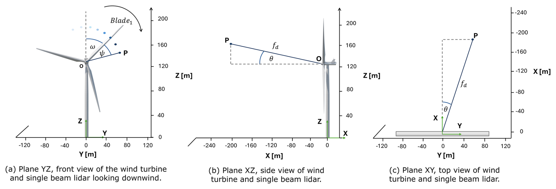
Figure 3 Left-handed coordinate system for a single-beam lidar mounted on the DTU 10 MW RWT. Example with range length f_d=200 m, half-cone angle θ=20°, azimuthal angle ψ=30°, and blade 1 at ω=35°.

Therefore, the LOS velocity accounting for beam orientation and tilt can finally be expressed as

$$\begin{array}{ll}{\displaystyle }& {\displaystyle }{V}_{\text{LOS}}(\mathit{\theta },\mathit{\psi },\mathit{\omega }(t),\mathit{\beta },\mathit{P})=\\ {\displaystyle }& {\displaystyle }\left[\cos \right(\mathit{\beta }\left)\cos \right(\mathit{\theta })-\sin (\mathit{\beta }\left)\sin \right(\mathit{\theta }\left)\cos \right(\mathit{\psi }+\mathit{\omega }\left(t\right)\left)\right]\cdot u\left(\mathit{P}\right)\\ {\displaystyle }& {\displaystyle }+\left[\sin \right(\mathit{\theta }\left)\sin \right(\mathit{\psi }+\mathit{\omega }\left(t\right)\left)\right]\cdot v\left(\mathit{P}\right)\\ \text{(6)}& {\displaystyle }& {\displaystyle }+\left[\sin \right(\mathit{\beta }\left)\cos \right(\mathit{\theta })+\cos (\mathit{\beta }\left)\sin \right(\mathit{\theta }\left)\cos \right(\mathit{\psi }+\mathit{\omega }\left(t\right)\left)\right]\cdot w\left(\mathit{P}\right).\end{array}$$

The longitudinal wind speed is estimated by projecting V_LOS onto the x axis. This projection assumes negligible lateral and vertical components (v and w) when the rotor is perfectly aligned with the wind (Schlipf et al., 2013; Simley et al., 2011), which introduces cross-contamination errors (Kelberlau and Mann, 2020). The final equation to project the LOS velocity to the longitudinal direction is thus as follows:

$$\begin{array}{ll}{\displaystyle }& {\displaystyle }{u}_{\text{lidar}}(\mathit{\theta },\mathit{\psi },\mathit{\omega }(t),\mathit{\beta },\mathit{P})=\\ \text{(7)}& {\displaystyle }& {\displaystyle \frac{V_{\text{LOS}}(\mathit{\theta },\mathit{\psi },\mathit{\omega }(t),\mathit{P})}{\cos \left(\mathit{\beta }\right)\cos \left(\mathit{\theta }\right)-\sin \left(\mathit{\beta }\right)\sin \left(\mathit{\theta }\right)\cos (\mathit{\psi }+\mathit{\omega }(t\left)\right)}}.\end{array}$$

Note that the projection is performed from the lidar origin O, placed at $(-L_{\mathrm{s}},\mathrm{0},Z_{\text{hub}})$, and therefore the projection is only affected by the rotation matrix R_hub.

Effects related to optics, internal signal processing, and lidar-specific smearing are not considered in this study.

2.5 Lidar scanning strategy

The HAWC2 hub-lidar sensor supports flexible scanning configurations, allowing multiple beams with user-defined half-cone angles (θ), azimuthal angles (ψ), and range lengths (f_d). In this study, a six-beam configuration is employed, with each beam sampled sequentially at 5 Hz and no switching delay. The lidar records 29 fixed range gates spaced every 10 m, covering distances from 70 to 350 m – consistent with common pulsed lidar practice (Peña et al., 2013). During post-processing, the beam sequence, sampling frequency, and switching delay can be customized.

Preliminary analysis (not shown for brevity) revealed that reconstruction accuracy improves when all six lidar beams are angled away from the central axis, rather than having a central beam pointing directly upwind. Although each beam samples multiple range gates, a beam aligned with the wind direction collects data along a nearly straight line, with only a slight vertical shift due to turbine tilt. As a result, many measurements overlap and map into the same grid location, providing only a small number of central points in the fixed spatial grid. In contrast, angled beams increase their spatial coverage and provide more data for the estimation across the rotor plane. Similar results have been reported by Simley et al. (2014), where optimal scan radii were found to be approximately 70 %–75 % of the rotor span.

The half-cone angle selection affects both projection errors – due to the assumption of negligible v and w components – and the spatial coverage of the rotor. Increasing the preview distance reduces cross-contamination and induction effects but increases errors due to wind evolution (Simley et al., 2012). Since HAWC2 does not model induction in the lidar sensor or temporal evolution of inflow, their impact is therefore not considered in this study.

The azimuthal angle defines each beam's angular separation from blade 1 in the rotating frame (Fig. 3), with allowable values in this study, $\mathit{\psi }\in [\mathrm{0}\mathit{°},\mathrm{120}\mathit{°},\mathrm{240}\mathit{°}]$, based on practical installation constraints. Specifically, for many multi-megawatt wind turbines, manufacturers provide access to the hub through service hatches positioned every 120°. Aligning the lidar beams with these access points simplifies both the installation and the maintenance processes.

The goal is to optimize the beam sequence to maximize rotor plane coverage over a given number of scans, where a “scan” is defined as the time needed to sample all six beams. At 5 Hz per beam, a single scan takes t_scan=1.2 s.

Figure 4 illustrates the final six-beam hub-lidar configuration, which was found with an exhaustive search through iteration at fixed rotor speed Ω=9.6 rpm (rated speed of the DTU 10 MW turbine), yielding the following optimal beam sequence: $\mathit{\psi }=[\mathrm{0}\mathit{°},\mathrm{240}\mathit{°},\mathrm{120}\mathit{°},\mathrm{240}\mathit{°},\mathrm{120}\mathit{°},\mathrm{0}\mathit{°}]$. Panel (a) shows the initial mounting azimuthal angles (YZ view), (b) the scanning trajectory over one scan (non-rotating frame), and (c) beam locations onto the XZ plane. This azimuthal configuration ensures optimal coverage of the rotor area above rated wind speed, since this is the operational range where LAC is used for load reduction.

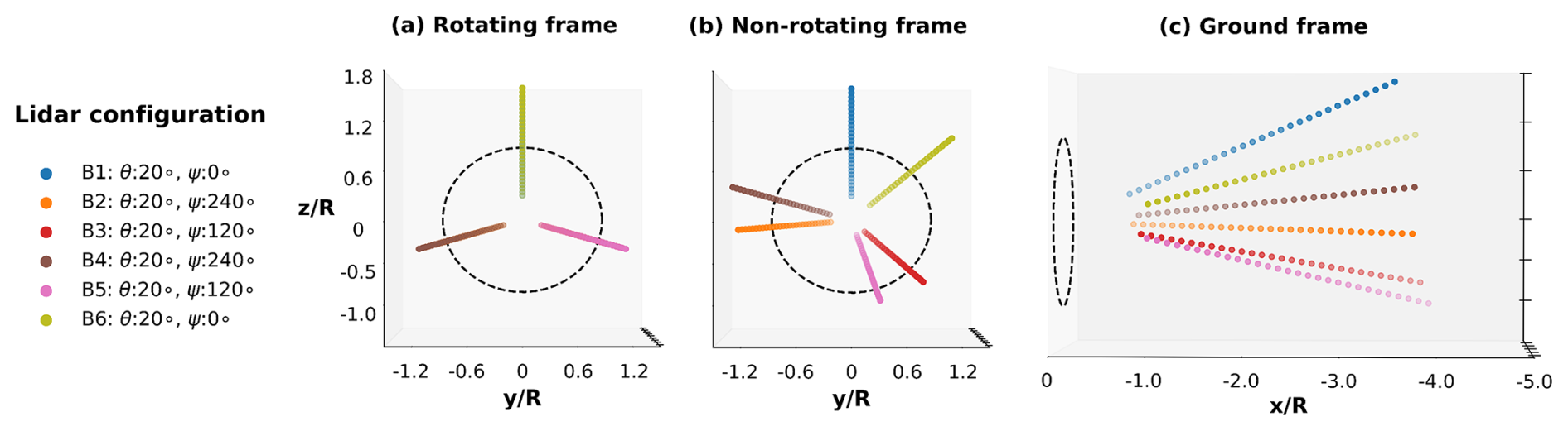
Figure 4 Six-beam lidar configuration with a half-cone angle θ=20° for all beams, azimuthal angles $\mathit{\psi }=[\mathrm{0}\mathit{°},\mathrm{240}\mathit{°},\mathrm{120}\mathit{°},\mathrm{240}\mathit{°},\mathrm{120}\mathit{°},\mathrm{0}\mathit{°}]$, and 29 range gates from 70 to 350 m spaced every 10 m. (a) Initial beam mounting positions (YZ view), (b) scanning trajectory over one scan at Ω=9.6 rpm, and (c) beam locations on the XZ plane. The dashed black circle indicates the DTU 10 MW RWT rotor (R=89 m).

2.6 Measurement selection for reconstruction

Synthetic lidar measurements are extracted from the reference inflow fields (Sect. 2.2) using the hub-lidar sensor. During post-processing, the 20 Hz HAWC2 lidar output is downsampled to a 5 Hz sampling rate per beam, with no switching delay.

Measurements used for the reconstruction are selected through a spatial filtering process. In the lateral and vertical directions, the filter dimensions match those of the turbulence box from set A (refer to Sect. 2.2). In the longitudinal direction, the filter spans a distance $d_{\text{span}}={\overline{U}}_{\mathrm{o}}{n}_{\text{scan}}{t}_{\text{scan}}$, where n_scan is the selected number of scans, and t_scan=1.2 s is the duration of a single full scan. This longitudinal span is centered around the target reconstruction plane, located at $X_{\text{target}}={\overline{U}}_{\mathrm{o}}{t}_{\mathrm{s}}$, where t_s denotes the time step at which the reconstruction is evaluated. As a result, only measurements satisfying the condition $X_{\text{target}}-\frac{\mathrm{1}}{\mathrm{2}}{\overline{U}}_{\mathrm{o}}{n}_{\text{scan}}{t}_{\text{scan}}<x<X_{\text{target}}+\frac{\mathrm{1}}{\mathrm{2}}{\overline{U}}_{\mathrm{o}}{n}_{\text{scan}}{t}_{\text{scan}}$ are selected for the reconstruction. Additionally, we imposed a constraint requiring all selected measurements to be located at least 1 s upstream of the rotor plane to ensure preview time.

This process is illustrated in Fig. 5, where (a) shows lidar data advancing towards the rotor with the cuboid centered around X_target, representing the spatial filtering region, and (b) maps selected measurements inside the cuboid onto the fixed YZ grid. If multiple measurements fall into the same grid cell, only the one closest to X_target is retained. Panel (c) shows the resulting fluctuations after subtracting the known shear profile ($\overline{U}(y,z)$) from the LES dataset set A (refer to Sect. 2.2).

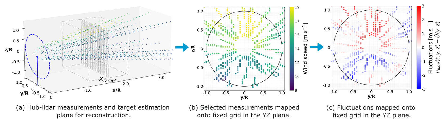
Figure 5 Lidar measurement selection for wind field reconstruction at a single time step. (a) Lidar data advancing toward the rotor with the spatial filtering cuboid centered at $X_{\text{target}}={\overline{U}}_{\mathrm{o}}{t}_{\mathrm{s}}$. (b) Mapping onto a fixed YZ grid. (c) Subtraction of the vertical wind speed profile. The dashed black circle in plots (b) and (c) indicates the DTU 10 MW RWT rotor (R=89 m).

All data used in this study are gather in a publicly available dataset (Soto Sagredo et al., 2025a).

2.7 Wind inflow reconstruction techniques

This section presents the methodologies used to reconstruct the longitudinal wind component (u) from synthetic lidar measurements obtained from the hub-lidar database (Sect. 2.6). Reconstructions are performed on a fixed 39×91 grid (y×z), consistent with the global POD modes (Sect. 2.2). A total of 1200 time steps (600 s) are reconstructed with a sampling interval of d_t=0.5 s.

All four methods use lidar-derived wind speed fluctuations as input, defined as $u_{\text{lidar}}^{\prime }(t,y,z)=u_{\text{lidar}}(t,y,z)-\overline{U}(y,z)$, where $\overline{U}(y,z)$ is the known mean vertical wind speed profile (i.e., shear) from LES set A. This step standardizes the input across methods. After reconstructing the fluctuating component, the known shear is readded to obtain the full wind field for evaluation.

The four reconstruction techniques evaluated in this study are described below.

2.7.1 Baseline

The baseline methodology replicates the standard approach of estimating REWS from lidar measurements in LAC applications (Held and Mann, 2019). To ensure fair comparison, we account for the known shear profile. The reconstructed longitudinal wind speed at each time step is defined as

$$\begin{array}{}\text{(8)}& {\displaystyle }{\displaystyle }u(t,y,z)={\displaystyle \frac{\mathrm{1}}{n_{\text{meas}}}}\sum _{i=\mathrm{1}}^{n_{\text{meas}}}{u}_{\text{lidar},i}^{\prime }+\overline{U}(y,z),\end{array}$$

where $u_{\text{lidar},i}^{\prime }$ is the LOS-projected wind speed fluctuation (Sect. 2.4) within the circular region A_R defined by $[y_j^{\mathrm{2}}+(z_j-Z_{\text{hub}}{)}^{\mathrm{2}}{]}^{\mathrm{1}/\mathrm{2}}\le \mathrm{95}$ m, centered at hub height in the fixed YZ grid plane (Fig. 5c). This area spans the rotor disk of the DTU 10 MW turbine with a 6 m margin to account for tower and shaft motion. The term n_meas denotes the number of lidar measurements available within the circular area A_R in the fixed plane.

2.7.2 Least-squares fit of POD modes

The Moore–Penrose pseudo-inverse is used to solve a least-squares problem for estimating the modal time series from lidar measurements, originally introduced by Moore (1920) and independently by Penrose (1955).

Using the projected LOS fluctuations, $u_{\text{lidar}}^{\prime }$, this field is stored in a matrix ${\mathbf{M}}_{\text{lidar}}\in {\mathbb{R}}^{N_y\times N_z}$ on a regular YZ grid (Fig. 5c), with missing data points assigned NaN for numerical computational purposes, where N_y=39 and N_z=91 are the grid points across the lateral and vertical directions respectively. We define the index set $\mathcal{I}=\mathit{\{}{i}_{\mathrm{1}},i_{\mathrm{2}},\mathrm{\dots },i_{n_{\text{meas}}}\mathit{\}}$ for grid locations with valid measurements, where n_meas is the number of available measurements. Hence, the measurement vector D_lidar is defined as ${\mathit{D}}_{\mathrm{lidar}}=\text{vec}({\mathbf{M}}_{\text{lidar}}{)}_{\mathcal{I}}\in {\mathbb{R}}^{n_{\text{lidar}}}$, where vec(⋅) denotes column-wise vectorization.

The global POD modes G are sub-sampled at ℐ locations, and the first K global POD modes are selected to form the matrix $\mathbf{A}={\mathbf{G}}_{\mathcal{I},\mathrm{1}:K}\in {\mathbb{R}}^{n_{\text{meas}}\times K}$.

The modal coefficients $\stackrel{\mathrm{̃}}{\mathit{\varphi }}$ are computed by solving the least-squares problem via the pseudo-inverse of A by projecting D_lidar onto the column space of A, leading to $\stackrel{\mathrm{̃}}{\mathit{\varphi }}=({\mathbf{A}}^{\top }\mathbf{A}{)}^{-\mathrm{1}}{\mathbf{A}}^{\top }{\mathit{D}}_{\mathrm{lidar}}$. The reconstructed wind field at each time step is then computed as

$$\begin{array}{}\text{(9)}& {\displaystyle }{\displaystyle }u(t,y,z)=\sum _{i=\mathrm{1}}^K{g}_i(y,z){\stackrel{\mathrm{̃}}{\mathit{\varphi }}}_i\left(t\right)+\overline{U}(y,z),\end{array}$$

where g_i(y,z) is the ith POD mode and ${\stackrel{\mathrm{̃}}{\mathit{\varphi }}}_i\left(t\right)$ the corresponding estimated modal amplitude. Finally, the known mean profile $\overline{U}(y,z)$ is readded to recover the full field.

2.7.3 Interpolation with IDW

IDW estimates the wind fluctuations at a target location as a weighted average of nearby measurements, where influence decreases with distance. If the target coincides with a measurement location, the interpolated value matches the measurement. Mathematically, the interpolated longitudinal velocity at position $\mathit{x}=(t,y,z)$ is calculated as

$$\begin{array}{}\text{(10)}& {\displaystyle }{\displaystyle }u(t,y,z)={\displaystyle \frac{{\sum }_{i=\mathrm{1}}^{n_{\text{meas}}}{w}_i\left(\mathit{x}\right)u_i^{\prime }}{{\sum }_{i=\mathrm{1}}^{n_{\text{meas}}}{w}_i\left(\mathit{x}\right)}}+\overline{U}(y,z),\end{array}$$

where $u_i^{\prime }$ is the wind speed fluctuation at measurement location x_i, and the weights w_i(x) are defined as

$$\begin{array}{}\text{(11)}& {\displaystyle }{\displaystyle }{w}_i\left(\mathit{x}\right)={\displaystyle \frac{\mathrm{1}}{d(\mathit{x},{\mathit{x}}_{\mathit{i}}{)}^p}},\end{array}$$

where d(x,x_i) is the Euclidean distance between the location of unknown u^′ and lidar measurements $u_i^{\prime }$, and p is a positive exponent controlling the decay rate, where higher values of p emphasize nearer points. An exponent of p=3 was found to minimize reconstruction errors.

2.7.4 Hybrid methodology: IDW combined with POD-LSQ

The final method combining IDW and POD-LSQ is presented in this section, called POD-IDW. First, the wind field fluctuations across the YZ plane are estimated at each time step using the IDW technique, following Sect. 2.7.3. Using the resulting IDW-reconstructed fluctuations (without the added vertical shear profile), the modal amplitudes $\stackrel{\mathrm{̃}}{\mathit{\varphi }}$ are then estimated by performing a least-squares fit onto the global POD modes (Sect. 2.7.2).

Therefore, the modal coefficients $\stackrel{\mathrm{̃}}{\mathit{\varphi }}$ are computed as $\stackrel{\mathrm{̃}}{\mathit{\varphi }}=({\mathbf{A}}^{\top }\mathbf{A}{)}^{-\mathrm{1}}{\mathbf{A}}^{\top }{\mathit{D}}_{\mathrm{IDW}}$, where ${\mathit{D}}_{\mathrm{IDW}}\in {\mathbb{R}}^{N_y\times N_z}$ is now the vectorization of the IDW reconstructed plane.

This hybrid approach is proposed to address a challenge encountered when using POD-LSQ: in areas without measurements, localized overfitting occurs. By using the IDW interpolated field to estimate the modal amplitudes, this limitation is mitigated.

2.8 Metrics for optimal parameter selection

Several parameters influence the accuracy of wind field reconstruction. To quantify the performance of the methods described in Sect. 2.7, we use the mean absolute error (MAE) computed within an area around the rotor, denoted as A_R (see Sect. 2.7.1). The MAE is computed over the 10 min simulation period (N_t=1200, d_t=0.5 s) as

$$\begin{array}{ll}{\displaystyle }& {\displaystyle }{\text{MAE}}_{\text{rotor},i,m}(\mathit{\theta },n_{\text{scan}},K)={\displaystyle \frac{\mathrm{1}}{N_t}}\\ \text{(12)}& {\displaystyle }& {\displaystyle }\times \sum _{t=\mathrm{1}}^{N_t}\left[{\displaystyle \frac{\mathrm{1}}{N}}\sum _{(y,z)\in A_R}\left|u_{\text{ref},i}(t,y,z)-u_{i,m}(t,y,z)\right|\right],\end{array}$$

where N is the number of spatial grid points within the rotor area A_R, and u_ref,i denotes the reference wind field for inflow case i. The index $i\in \mathit{\{}\mathrm{1},\mathrm{\dots },N_{\text{cases}}\mathit{\}}$ spans the set of inflow cases, with N_cases=64 representing 16 independent 10 min realizations across four wind speeds ${\overline{U}}_{\mathrm{o}}\in \mathit{\{}\mathrm{8.0},\mathrm{12.0},\mathrm{15.0},\mathrm{20.0}\mathit{\}}\mathrm{m}{\mathrm{s}}^{-\mathrm{1}}$. The subscript m represents each reconstruction method described in Sect. 2.7, with m∈{Baseline, POD-LSQ, IDW, and POD-IDW}.

To enable fair comparison across different wind speeds, all reconstruction errors are normalized by the corresponding inflow mean wind speed ${\overline{U}}_{\mathrm{o},i}$. The global performance metric for a given method m is defined as

$$\begin{array}{ll}{\displaystyle }& {\displaystyle }{\text{MAE}}_{\text{global},m}(\mathit{\theta },n_{\text{scan}},K)={\displaystyle \frac{\mathrm{1}}{N_{\text{cases}}}}\\ \text{(13)}& {\displaystyle }& {\displaystyle }\times \sum _{i=\mathrm{1}}^{N_{\text{cases}}}\left({\displaystyle \frac{{\text{MAE}}_{\text{rotor},i,m}(\mathit{\theta },n_{\text{scan}},K)}{{\overline{U}}_{\mathrm{o},i}}}\right).\end{array}$$

The global reconstruction performance depends on several key parameters. First, the half-cone opening angle θ directly influences the spatial distribution and availability of lidar measurements across the rotor, as well as potential cross-contamination effects. In this study, we evaluate θ values in the range $\mathit{\theta }\in \mathit{\{}\mathrm{10.0}\mathit{°},\mathrm{12.5}\mathit{°},\mathrm{\dots },\mathrm{50.0}\mathit{°}\mathit{\}}$, using the same angle for all six beams.

Second, the number of lidar measurements per time step, n_meas, depends on the selected number of lidar scans, $n_{\text{scan}}\in \mathit{\{}\mathrm{1},\mathrm{2},\mathrm{\dots },\mathrm{8}\mathit{\}}$ (see Sect. 2.6). Increasing n_scan provides higher data availability, but it can degrade reconstruction due to higher spatial filtering.

For POD-based methods, the number of retained modes K is another important parameter. A higher K allows for finer-scale flow reconstruction but can increase sensitivity to measurement sparsity and lead to overfitting. We evaluate $K\in \mathit{\{}\mathrm{10},\mathrm{20},\mathrm{30},\mathrm{40},\mathrm{50},\mathrm{75},\mathrm{100},\mathrm{125},\mathrm{150},\mathrm{200}\mathit{\}}$.

The optimal parameter combination for each method, $({\mathit{\theta }}_{\text{opt},m},n_{\text{scan,opt},m},K_{\text{opt},m})$, is defined as the one that minimizes the global normalized reconstruction error:

$$\begin{array}{ll}{\displaystyle }& {\displaystyle }({\mathit{\theta }}_{\text{opt},m},n_{\text{scan,opt},m},K_{\text{opt},m})=\\ \text{(14)}& {\displaystyle }& {\displaystyle }\arg \underset{\mathit{\theta },n_{\text{scan}},K}{min}\left\{{\text{MAE}}_{\text{global},m}(\mathit{\theta },n_{\text{scan}},K)\right\},\end{array}$$

where the search spans all 1360 ($\mathrm{17}\times \mathrm{8}\times \mathrm{10}$) combinations in the discrete parameter space.

3 Results

To evaluate the performance and characteristics of the proposed reconstruction methods, we begin by assessing the accuracy of the modal amplitude estimation for POD-LSQ using lidar measurements, as discussed in Sect. 3.1. We then examine how the number of scans and modes influences the spectral content of the reconstructed inflow fields in Sect. 3.2. The effect of the half-cone opening angle on reconstruction accuracy is analyzed in Sect. 3.3, while Sect. 3.4 investigates the influence of wind speed quantity. Finally, Sect. 3.5 synthesizes these findings and presents a discussion on the optimal parameter configuration for each method.

To assess the influence of wind speed quantity selection on reconstruction accuracy, we compare the reconstruction results using three wind speed quantities, hereafter referred to as (i) the volume-averaged lidar estimate, u_{lidar, wgh}, representing LOS velocities projected into the longitudinal direction and averaged over the lidar probe volume; (ii) the nominal lidar estimate, u_{lidar, nom}, obtained from the same projection procedure but without applying volume averaging; and (iii) the true wind speed, u_fw, corresponding to the reference longitudinal wind velocity extracted from the reference LES inflow field at the same grid locations in the X_target plane where the lidar measurements are fixed (see Fig. 5c) at each time step.

While only u_{lidar, wgh} represents a physically realistic lidar input, the alternative wind speed definitions are used for diagnostic purposes. In particular, u_fw isolates the performance of the reconstruction methods from key sources of measurement uncertainty, including volume averaging, cross-contamination, tower motion, and multi-distance fixed-plane mapping error. The latter refers to the spatial inconsistency introduced when lidar measurements – collected at different longitudinal positions – are projected onto a fixed estimation plane (X_target), ignoring their true spatial separation along the longitudinal direction. In contrast, the difference between u_{lidar, nom} and u_{lidar, wgh} isolates the effect of volume averaging alone. These three wind speed definitions are used consistently throughout the paper to evaluate reconstruction accuracy and quantify the impact of measurement-related uncertainties.

3.1 Modal amplitude estimation with POD-LSQ

In real-time applications, reconstructing wind fields at each time step using global POD modes requires estimating the corresponding modal amplitudes, $\stackrel{\mathrm{̃}}{\mathit{\varphi }}\left(t\right)$. This estimation is carried out using the POD-LSQ approach described in Sect. 2.7.2. In this section, we evaluate how wind speed quantity selection affects the accuracy of these modal amplitude estimations.

Figure 6 presents the first five modal amplitudes for a representative 10 min inflow case with a mean wind speed of ${\overline{U}}_{\mathrm{o}}=\mathrm{15.35}\mathrm{m}{\mathrm{s}}^{-\mathrm{1}}$. The reference modal amplitudes (solid black lines) are compared against those estimated by POD-LSQ (dashed orange lines), using K=50 global POD modes, n_scan=7 scans, and a half-cone angle of θ=22.5°. The top row of Fig. 6 shows results obtained using the true wind speed as input, while the second row uses the nominal lidar estimate (without volume averaging), and the bottom row uses the volume-averaged lidar estimate. This comparison allows us to isolate and quantify the impact of measurement errors on the estimation of modal amplitudes. Each subplot also reports the normalized MAE, defined as $\text{MAE}/\mathit{\sigma }$, where σ is the standard deviation of the corresponding reference amplitude.

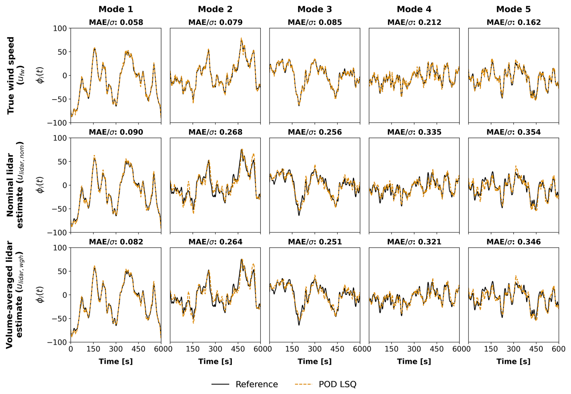
Figure 6 First five modal amplitudes estimated using POD-LSQ with K=50 global POD modes, n_scan=7 scans, and half-cone angle θ=22.5°. Top row: estimation using true wind speed (u_fw), second row: estimation using nominal lidar-estimated (u_{lidar, nom}) wind speed, and bottom row: estimation using volume-averaged lidar-estimated (u_{lidar, wgh}) wind speed.

As expected, the estimation error $\text{MAE}/\mathit{\sigma }$ increases with mode number. Lower-order modes (e.g., modes 1–3), which represent dominant large-scale structures, are reconstructed more accurately than higher-order modes (e.g., modes 4–5), which correspond to finer-scale features. Furthermore, the use of the lidar-based estimates leads to consistently higher reconstruction errors compared to using the true wind speed. For mode 1, $\text{MAE}/\mathit{\sigma }$ increases by 55 % when using the nominal lidar estimate compared to the true wind speed, while an increase of 41 % is observed for the volume-averaged lidar estimate. For mode 5, these differences become more pronounced, with increases of 119 % and 114 %, respectively. These results highlight the sensitivity of modal amplitude estimation to measurement-related uncertainties – such as cross-contamination, spatial offsets resulting from the fixed-grid filtering approach used for multi-distance lidar measurements, and tower-induced motion. Higher-order modes are particularly affected by these effects. Notably, probe volume averaging helps to reduce such errors, as reflected in the consistently lower $\text{MAE}/\mathit{\sigma }$ values compared to the nominal case.

3.2 Sensitivity to number of scans and modes on the spectral content

To assess how the number of scans and modes affects the reconstruction of turbulent inflow fields, we analyze the power spectral density (PSD) of the u velocity fluctuations for a representative case with ${\overline{U}}_{\mathrm{o}}=\mathrm{15.35}\mathrm{m}{\mathrm{s}}^{-\mathrm{1}}$ over a 10 min simulation. The PSD is estimated using Welch's method with a Hamming window, six segments, and 50 % overlap. To characterize the spectral energy content across the full rotor plane rather than just the rotor-averaged wind speed, the PSD is computed point-wise and subsequently averaged over all grid points within the area A_R (refer to Sect. 2.7.1):

$$\begin{array}{}\text{(15)}& {\displaystyle }{\displaystyle }{\text{PSD}}_{\text{avg}}\left(f\right)={\displaystyle \frac{\mathrm{1}}{N_{\text{grid}}}}\sum _{i=\mathrm{1}}^{N_{\text{grid}}}{S}_{ii}\left(f\right),\end{array}$$

where S_ii(f) is the power spectrum estimated at grid point i∈A_R, and N_grid is the total number of grid points inside A_R.

3.2.1 Number of scans and estimation method

This section compares the PSD of the original flow to the estimated flow for different estimation methods and numbers of scans. The number of modes used in the POD-based estimation methods is kept fixed for this analysis; the impact of POD modes is analyzed in detail in Sect. 3.2.2.

Figure 7 presents the PSD results for (a) baseline, (b) POD-LSQ, (c) IDW, and (d) POD-IDW, using θ=22.5° and K=100 global POD modes. Each panel shows reconstructions for various numbers of lidar scans ($n_{\text{scan}}\in \mathit{\{}\mathrm{4},\mathrm{8},\mathrm{12},\mathrm{16}\mathit{\}}$) and two types of wind speed inputs: the true wind speed (u_fw, solid lines) and the volume-averaged lidar estimate (u_{lidar, wgh}, dashed lines). For reference, the full LES turbulence spectrum is plotted in solid black. The truncated POD spectrum (gray dashed) corresponds to the projection of the LES flow onto the first 100 POD modes using the standard inner product, which is a better basis of comparison for the POD methods. The vertical dashed line indicates the tower's first fore–aft eigenfrequency, f_tower. The energy drop-off beyond 0.1 Hz in the LES reference is attributed to grid resolution limitations, as reported in Thedin et al. (2023), Doubrawa et al. (2019), and Rivera-Arreba et al. (2022). Similarly, the further roll-off observed in the truncated POD spectrum is due to modal truncation. As noted by Liverud Krathe et al. (2025), these high-frequency limitations do not significantly affect fatigue analysis outcomes.

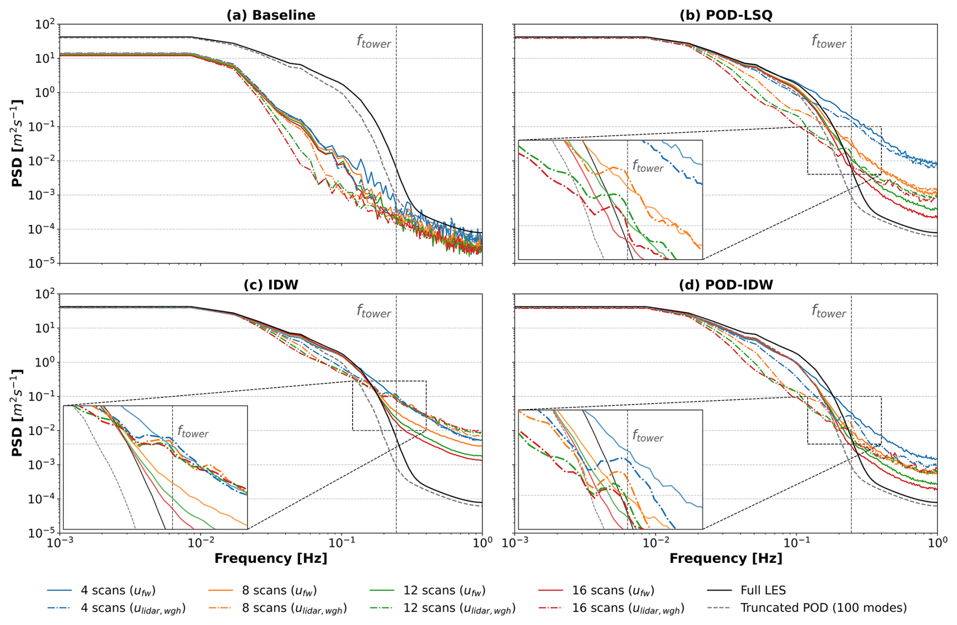
Figure 7 Influence of the number of scans n_scan on the turbulence spectra of the u component over a 10 min simulation for each method, using θ=22.5° and K=100 global POD modes for POD-based methods, with the true wind speed (u_fw) and volume-averaged lidar estimate (u_{lidar, wgh}) as input parameters for the reconstruction. Welch's method with Hamming window (six segments, 50 % overlap) is applied, and the PSDs around the area A_R (see Sect. 2.7.1) around the rotor area are averaged for smoothing.

Low frequencies

At frequencies below 0.1 Hz, all reconstruction methods except the baseline (Fig. 7a) closely follow the LES spectrum when estimating using the true wind speed u_fw (solid lines). The baseline method is formulated as a rotor-equivalent estimate combined with the prescribed mean shear profile such that the time-varying component is spatially uniform across the rotor plane. Consequently, it does not reproduce spatially varying turbulent fluctuations at individual grid points within A_R. Because the spectra are obtained by averaging point-wise PSDs over all grid points inside A_R, the baseline's rotor averaging inherently reduces energy in the spatially resolved u spectra, including at low frequencies.

IDW effectively reproduces the LES spectrum, while POD-based methods align with the truncated POD reference, consistent with their basis truncation. In contrast, reconstructions based on the volume-averaged lidar estimate consistently exhibit lower energy from 0.02 Hz upwards. This reduced energy results from two sources of spatial filtering: the intrinsic averaging within the probe volume (Peña et al., 2017) and the measurement selection procedure, which maps multi-distance observations – taken at varying longitudinal positions – onto a fixed grid. This process smooths out turbulent fluctuations by blending information across different regions of the inflow. This filtering effect also impacts the baseline method, though to a lesser extent given its already-simplified reconstruction approach.

High frequencies

In the high-frequency range, the flow estimated using POD-LSQ, POD-IDW, and IDW has more energy than the LES flow for both u_fw and the volume-averaged lidar estimate. When using u_fw, increasing the scan count reduces this extra spectral energy for these methods, drawing their spectra closer to the LES reference. This reduction in high-energy content with higher scans is driven by the number of available measurements in the rotor plane, which increases with n_scan. For example, in this study, four scans correspond to approximately 15 % coverage of the YZ plane, while 16 scans increases that coverage to around 42 %. Having more measurements in the rotor plane reduces overfitting for the POD methods, which results in lower spectral energy for more scans. In IDW, a higher number of measurements increases spatial coverage, reducing gaps between data points. This leads to more accurate interpolation and lower reconstruction error.

However, for lidar-based inputs, the measurement selection procedure described in Sect.2.6 selects data points across varying longitudinal positions and maps them onto a fixed grid, which becomes increasingly extended as more scans are included. This introduces an additional spatial filtering effect, resulting in a sharper energy drop beyond 0.017 Hz. While IDW does not exhibit the same steep decline, this instead reflects increased noise due to higher multi-distance fixed-plane mapping errors, rather than improved reconstruction fidelity. Unlike POD-based methods, which enforce spatial coherence through a global modal basis, IDW does not incorporate spatial correlations between measurements, which can compromise accuracy, especially for irregularly distributed data (Li et al., 2020; Bokati et al., 2022). Furthermore, IDW assumes isotropic flow variations and is sensitive to outliers, making it more susceptible to errors caused by spatial separation. This behavior is further illustrated in the time series example for n_scan=16 shown in Appendix C.

Tower natural frequency

A secondary effect visible in Fig. 7 is the presence of a peak near the tower's natural frequency, f_tower=0.25 Hz, in the volume-averaged lidar estimate reconstructions (zoomed area). This is caused by tower-induced motion distorting the lidar measurements. The effect is particularly visible when n_scan=4k for k∈ℕ, since four scans approximately match the tower's oscillation period. The peak is more pronounced in POD-based reconstructions and less distinguishable in IDW due to IDW's elevated background spectral energy near f_tower.

3.2.2 Number of POD modes

This section demonstrates the impact of the number of POD modes on the estimation for the POD-LSQ and POD-IDW methods, where n_scan is kept constant.

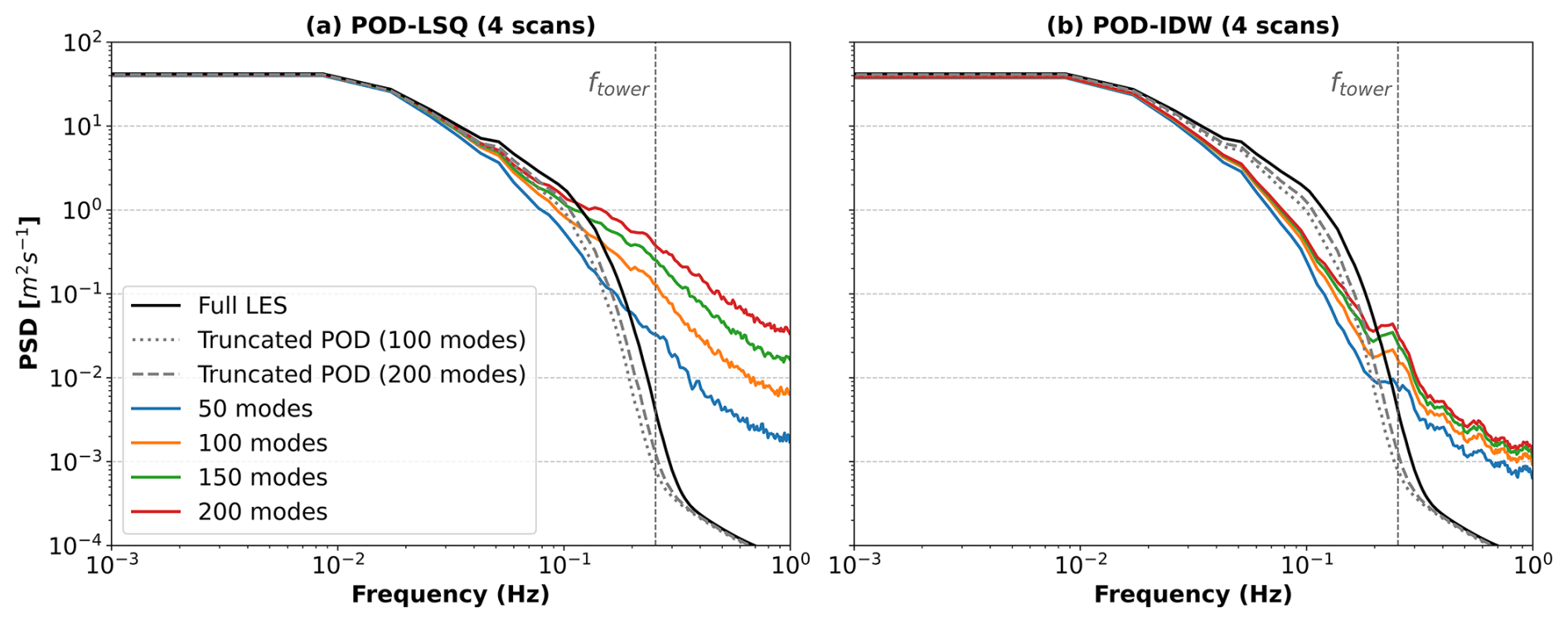
Figure 8 presents the PSD for (a) POD-LSQ and (b) POD-IDW for different numbers of modes, $K\in \mathit{\{}\mathrm{50},\mathrm{100},\mathrm{150},\mathrm{200}\mathit{\}}$, using n_scan=4, θ=22.5°, and the volume-averaged lidar estimate as input. Lower values of K capture the large-scale, low-frequency content of the flow, while increasing K introduces more high-frequency energy. At low frequencies, POD-LSQ aligns more closely with the truncated POD spectrum, whereas POD-IDW shows greater deviation due to the influence of the initial IDW plane, which introduces interpolation-related errors. At higher frequencies (above 0.1 Hz), POD-LSQ tends to overestimate energy, primarily due to overfitting in the modal amplitude estimation, as mentioned in Sect 3.2.1. This effect is discussed again in Sect. 3.3. POD-IDW mitigates overfitting by using the IDW-reconstructed plane as input for estimating modal amplitudes, which smooths the high-frequency content and reduces overfitting.

Figure 8 Influence of the number of POD modes (K) on the turbulence spectra of the u component over a 10 min simulation for POD-LSQ (a) and POD-IDW (b), with $K\in \mathrm{50},\mathrm{100},\mathrm{150},\mathrm{200}$ and n_scan=4. Welch's method is applied (six segments, 50 % overlap) over the interest area A_R (see Sect. 2.7.1).

3.2.3 Summary and methodological implications

The scan count, n_scan, exerts a dual influence on reconstruction quality. On the one hand, increasing n_scan improves fidelity when using ideal inputs (u_fw) by enhancing spatial coverage. On the other hand, it also increases the longitudinal separation between measurements, which can degrade reconstruction accuracy when lidar-based inputs (u_{lidar, wgh}) are used due to amplified multi-distance fixed-plane mapping error.

Each reconstruction method responds differently to this trade-off. IDW is particularly sensitive to spatial separation, as it does not account for spatial correlation across measurements. POD-LSQ, by contrast, is more affected by the number and distribution of available measurements – especially at higher values of K – since accurate estimation of modal amplitudes requires adequate spatial coverage. POD-IDW, which combines an initial IDW interpolation with subsequent POD fitting, inherits some limitations from the interpolation step but benefits from the modal projection, which helps to smooth errors introduced by spatial filtering (refer to Appendix C). As a result, the optimal selection of both scan count (n_scan) and number of POD modes (K) should be tailored to the specific sensitivities of each method and the nature of the available input.

Finally, attention should be given to the effects of tower motion, which introduce spurious energy near the tower's natural frequency (f_tower). These artifacts, particularly prominent in lidar-based reconstructions, require correction techniques or frequency-domain filtering to avoid negative impacts on both control performance and aeroelastic load assessments.

3.3 Effect of half-cone angle on reconstruction performance

The selection of the half-cone angle, θ, affects reconstruction accuracy in two main ways: (1) by influencing the number and spatial distribution of lidar measurements across the rotor plane and (2) by increasing cross-contamination in the volume-averaged lidar estimate derived from LOS measurements.

Figure 9 illustrates these effects at a representative time step across the YZ rotor plane. Each column corresponds to a half-cone angle $\mathit{\theta }\in \mathit{\{}\mathrm{10.0}\mathit{°},\mathrm{17.5}\mathit{°},\mathrm{20.0}\mathit{°},\mathrm{22.5}\mathit{°},\mathrm{35.0}\mathit{°},\mathrm{50.0}\mathit{°}\mathit{\}}$ using K=200 modes and n_scan=4 for all reconstructions. Row (a) shows the location of the lidar measurements, and each point's color represents the difference between the true wind speed (u_fw) and the volume-averaged lidar estimate (u_{lidar, wgh}), while rows (b)–(e) present reconstruction errors relative to the LES reference for (b) baseline, (c) POD-LSQ, (d) IDW, and (e) POD-IDW. MAE values are reported above each case.

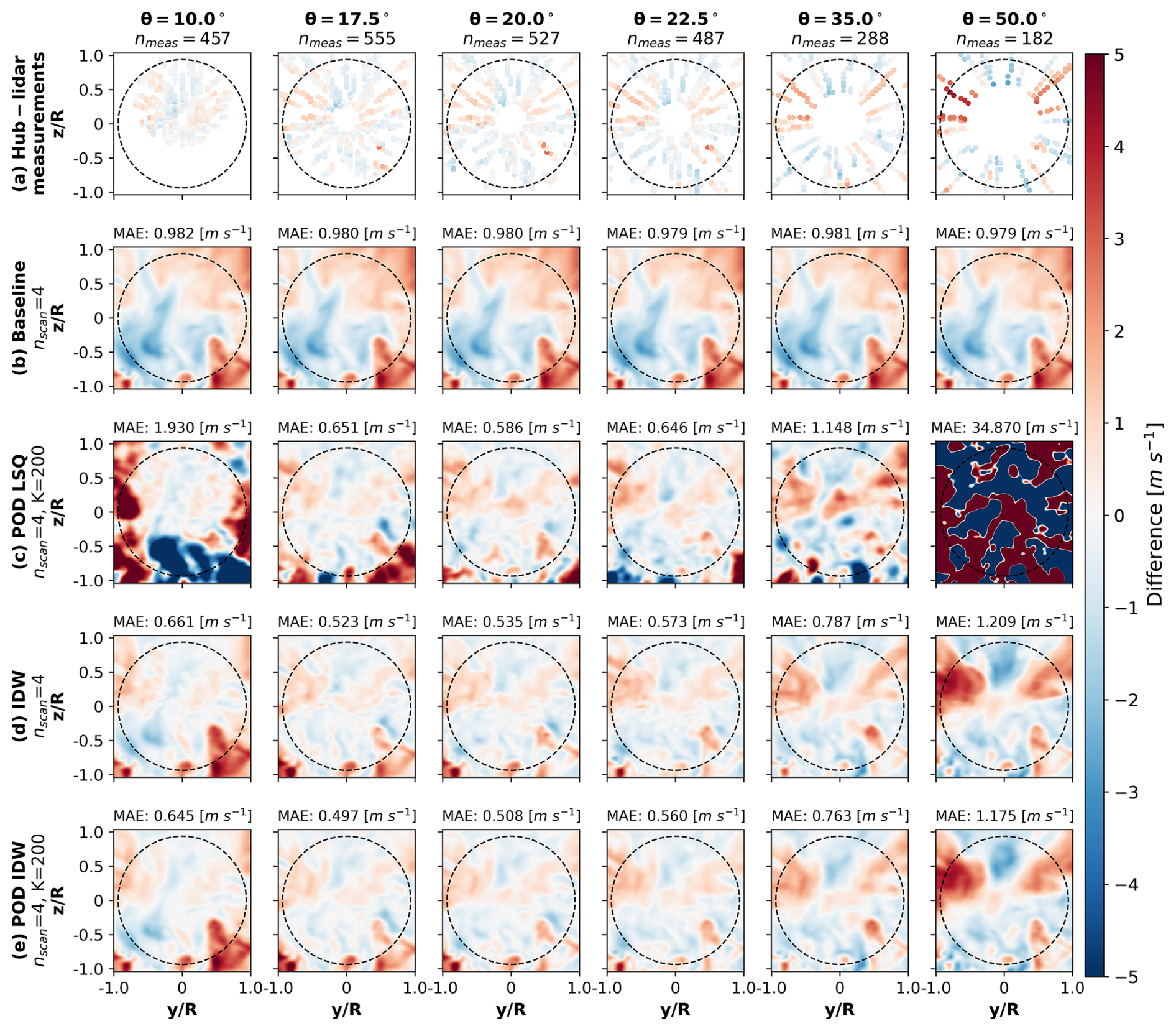
Figure 9 Difference across the YZ plane between the reconstructed ($u(t,y,z)$) and reference ($u_{\text{ref}}(t,y,z)$) wind fields for ${\overline{U}}_{\mathrm{o}}=\mathrm{15.35}\mathrm{m}{\mathrm{s}}^{-\mathrm{1}}$ at a single time step. The columns correspond to increasing half-cone angles from 10 to 50°, using four scans and 200 POD modes, where (a) shows the difference between the hub-lidar volume average projected LOS measurements (u_{lidar, wgh}) and the true wind speed (u_fw), and (b–e) present the differences between the reconstructed and LES reference cases for (b) baseline, (c) POD-LSQ, (d) IDW, and (e) POD-IDW. The blue colors indicate underestimation of wind speeds relative to the reference field, while the red colors indicate overestimation. The dashed black circle indicates the DTU 10 MW RWT rotor (R=89 m).

As shown in Fig. 9a, at θ=10.0°, measurements concentrate near the upper center of the rotor due to turbine tilt, yielding n_meas=457. With increasing θ, spatial coverage improves as measurements spread more broadly across the rotor plane. However, beyond a certain point, outer beams extend beyond the rotor, reducing central coverage. For example, at θ=50.0°, only 182 valid measurements remain as outer range gates extend beyond the rotor area due to beam inclination. Additionally, larger θ values increase cross-contamination – indicated by the more intense coloring of the points – due to increased misalignment with the line of sight and the longitudinal turbulence.

Figure 9b–e show how each method responds to changes in θ. The baseline method is relatively insensitive, exhibiting consistent performance across all angles. POD-LSQ, in contrast, is highly sensitive, as accuracy depends on both the number and the spatial distribution of measurements. At θ=10.0°, performance degrades despite a high measurement count due to poor spatial coverage and localized overfitting. At θ=50.0°, the number of measurements is too low (n_meas=182) to support fitting K=200 modes, yielding an underdetermined system and degraded accuracy. These results highlight that, for POD-based methods, ensuring n_meas≥K is necessary but not sufficient – broad spatial coverage is equally critical. Notably, although θ=10.0° yields more measurements than θ=35.0°, POD-LSQ performs worse, underscoring the importance of spatial distribution over raw measurement count.

The sensitivity of IDW and POD-IDW to θ is less significant than for POD-LSQ. However, both methods exhibit increased reconstruction error at θ=50.0°, consistent with greater cross-contamination in the LOS-derived wind speed (Fig. 9a). POD-IDW inherits interpolation errors from the IDW field, so spatial inaccuracies propagate into the final reconstruction. Still, applying POD over the IDW field reduces spatial inconsistencies, resulting in smoother fields and improved performance over IDW alone – though the improvement in MAE is limited (Fig. 9d and e).

Careful selection of the half-cone angle is therefore essential, particularly for POD-based methods. The angle must balance spatial coverage with minimal contamination from v and w components in the LOS signal. This selection depends on lidar geometry, turbine tilt, and alignment between beam orientation and the rotor plane. It is also critical to ensure that n_meas≥K and that measurements are sufficiently distributed to avoid overfitting in POD-LSQ. The baseline method, by contrast, remains largely insensitive to θ, provided enough data are collected across the scan radius (Simley et al., 2018).

3.4 Impact of wind speed quantity on reconstruction performance

To assess how lidar-induced measurement errors affects reconstruction accuracy, we evaluate each method using the three wind speed inputs: (i) true wind speed (u_fw), (ii) nominal lidar estimate without volume averaging (u_{lidar, nom}), and (iii) volume-averaged lidar estimate (u_{lidar, wgh}).

Figure 10 shows the global reconstruction error, MAE_global (defined in Sect. 2.8), as a function of the half-cone angle θ for each method using its optimal configuration, n_scan,opt and K_opt, determined as shown in Fig. 2 and listed in Table 1. Results are presented for four methods – (a) baseline, (b) POD-LSQ, (c) IDW, and (d) POD-IDW – under all three wind speed inputs. The performance spread across these inputs reflects the influence of measurement errors and volume averaging. A more comprehensive sensitivity analysis over θ, n_scan, and (where applicable) K, including the full set of heat maps used to identify the method-specific optima, is provided in Appendix D.

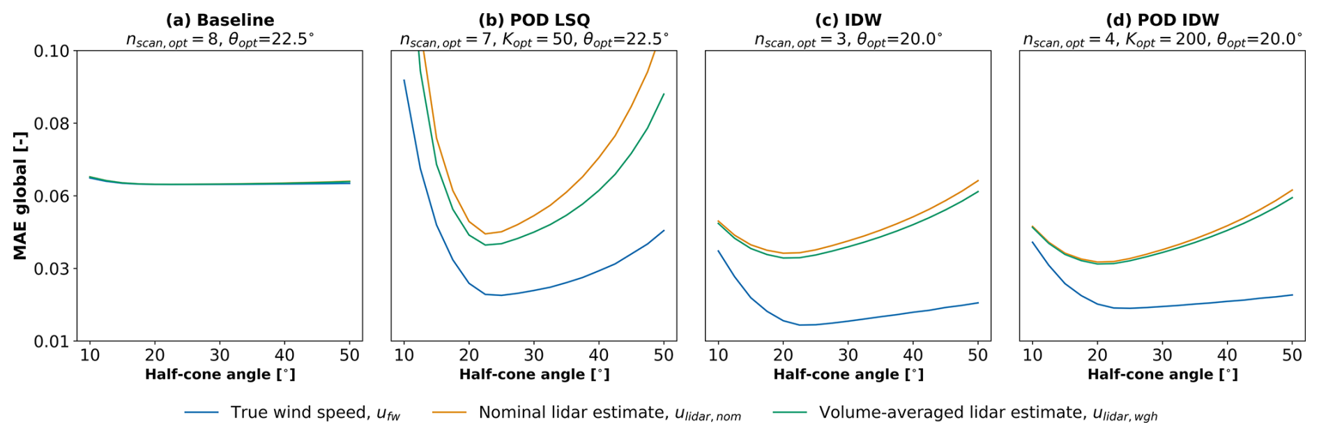
Figure 10 Global mean absolute error, MAE_global, as a function of half-cone angle, θ, for the best-performing configurations: (a) baseline, (b) POD-LSQ, (c) IDW, and (d) POD-IDW. Results are shown using true wind speed (u_fw, blue), nominal estimate (u_{lidar, nom}, orange), and volume-averaged estimate (u_{lidar, wgh}, green).

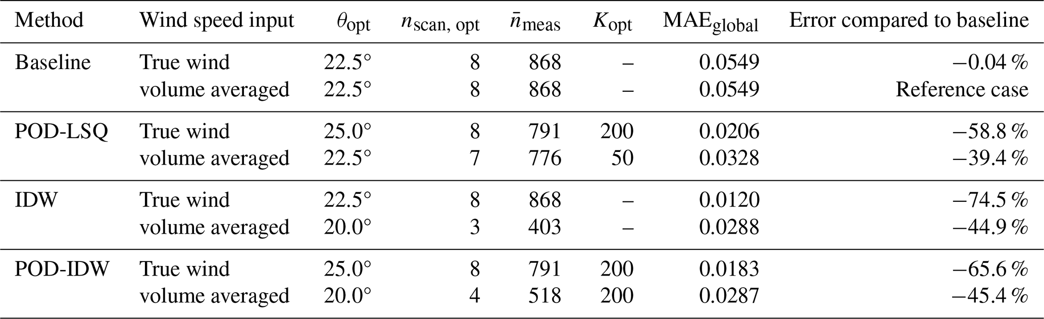
Table 1 Optimal parameter combinations $({\mathit{\theta }}_{\text{opt}},n_{\text{scan,opt}},K_{\text{opt}})$ that minimize the global mean absolute error, MAE_global, for each reconstruction method, using as inputs the true wind speed (u_fw) and volume-averaged lidar-estimated wind speed (u_{lidar, wgh}).

Consistent with Sect. 3.3, the baseline method (Fig. 10a) shows almost identical results regardless of input type due to its rotor-averaging approach that inherently smooths spatial uncertainties. Overall, the baseline yields larger reconstruction errors than the spatial reconstruction methods across most of the parameter space; however, for extreme half-cone angles, POD-LSQ can perform worse than the baseline. Among the other methods, POD-LSQ remains the most sensitive to half-cone angle selection, with errors increasing sharply as θ deviates from the optimum due to overfitting and cross-contamination, which impair modal amplitude estimation (see also Sect. 3.2 and 3.3). In contrast, IDW and POD-IDW show less sensitivity to θ, with errors remaining relatively stable even as measurement distribution deteriorates. For POD-IDW, this robustness is partly inherited from IDW, as it uses the interpolated IDW field for modal fitting and thus avoids overfitting (see Sect. 3.3).

IDW shows the largest performance gap between u_fw and lidar-based inputs, highlighting its strong sensitivity to uncertainties, particularly the multi-distance fixed-plane mapping error and cross-contamination. POD-IDW performs slightly better, as the modal decomposition enforces spatial coherence, mitigating some interpolation-related errors. POD-LSQ also benefits from modal constraints, reducing sensitivity to input uncertainty, though it remains highly dependent on θ.

Across all methods, reconstructions using the true wind speed u_fw significantly outperform those from the two line-of-sight quantities, but the volume-averaged input (u_{lidar, wgh}) outperforms the nominal lidar estimates (u_{lidar, nom}). In other words, there is a significant increase in error caused by measurement inaccuracies, but adding volume averaging actually reduces the error. This demonstrates the benefit of modeling the probe volume, as volume averaging reduces cross-contamination and improves reconstruction quality – a trend especially evident for POD-LSQ and consistent with the findings reported in Soto Sagredo et al. (2025b).

In summary, reconstruction accuracy is significantly influenced by measurement quantity. IDW is the most affected, followed by POD-IDW, which inherits interpolation errors. POD-LSQ shows better resilience but depends strongly on appropriate angle selection. The baseline, though robust to measurement variations, performs worst overall. These results emphasize the importance of tuning method-specific parameters for reliable lidar-based wind field reconstruction.

3.5 Overall method performance

The ultimate conclusion we would like to draw is which of the investigated methods performs “best”. The optimal parameter sets – half-cone angle θ_opt, number of scans n_scan,opt, and number of POD modes K_opt – are those that minimize the global mean absolute error MAE_global for each reconstruction method (Sect. 2.8). These values are summarized in Table 1 for both the true wind speed input (u_fw) and the volume-averaged lidar estimate (u_{lidar, wgh}), with corresponding performance trends shown in Fig. 10.

Using lidar-based input, POD-IDW achieves the lowest reconstruction error, with a 45.4 % reduction in MAE_global compared to the baseline. IDW performs nearly as well (44.9 % reduction), followed by POD-LSQ (39.4 %). With true wind input, IDW achieves the best accuracy (74.5 % reduction), followed by POD-IDW (65.6 %) and POD-LSQ (58.8 %). For the baseline, only a negligible 0.04 % difference exists between input types – reflecting its robustness to uncertainty but also its limited resolution, which results in the highest reconstruction error overall. Note that the baseline method achieves its best performance with n_scan=8, although using fewer scans results in nearly identical accuracy. This insensitivity to scan count reflects the inherent spatial averaging of the baseline approach.

Measurement errors – including probe volume averaging, cross-contamination, multi-distance fixed-plane mapping error, and tower motion – degrade reconstruction accuracy for all methods except the baseline. This effect is most pronounced for IDW (Sect. 3.2–3.4), where the error reduction drops from 74.5 % (with u_fw) to 44.9 % (with u_{lidar, wgh}), and the optimal number of scans decreases from eight to three. These shifts reflect IDW's strong sensitivity to the assumption that all selected measurements lie on the same plane, neglecting their actual longitudinal location in space. For all methods, using true wind input generally shifts the optimal half-cone angle θ upward by 2.5–5°, as cross-contamination is no longer a limiting factor. POD-LSQ, in particular, improves its performance by increasing the number of modes from 50 to 200 with only one additional scan, highlighting the impact of measurement uncertainty on modal amplitude estimation (Sect. 3.1).

Overall, POD-IDW offers the best reconstruction accuracy with lidar-based inputs but comes with a higher computational cost. IDW is simpler and moderately expensive but does not capture spatial correlations and assumes isotropic flow variations, leading to unrealistic estimates under certain conditions. POD-LSQ provides a good balance between accuracy and efficiency but requires careful tuning of lidar configuration and POD parameters. The baseline method is the fastest and most robust to measurement uncertainty, yet consistently delivers the poorest reconstruction quality. Ultimately, reliable wind field reconstruction depends on accounting for measurement uncertainty and appropriately tuning method-specific parameters.

4 Discussion

The goal of this study was to assess the reconstruction accuracy and robustness of three methods under semi-realistic inflow conditions, using LES-generated data and a hub-mounted lidar simulator. Evaluation was based on a global metric, MAE_global, which quantifies the deviation from the true inflow field across multiple conditions. While effective for identifying optimal parameters and quantifying deviations from the reference wind field, this metric does not capture the ability of the reconstructed fields to drive realistic turbine dynamics. A more robust analysis would involve evaluating the reconstruction error on turbine load channels, which is the subject of future work.

The current study makes several simplifying assumptions due to limitations in the available tools. Notably, the HAWC2 lidar implementation does not account for turbulence evolution (Bossanyi, 2013; de Maré and Mann, 2016) or induction effects (Borraccino et al., 2017; Mann et al., 2018), as it is based on Taylor's frozen turbulence hypothesis and BEM-based inflow dynamics. As a result, the inflow is treated as a stationary free-stream field, from where the lidar measurements are extracted. Although this is not realistic, it provides a controlled environment to evaluate reconstruction accuracy. Future work should incorporate 4D inflow fields from LES simulations that include these effects to better evaluate how they influence reconstruction performance – and how they may be compensated for in practice.

All methods in this study also rely on knowledge of the mean shear profile to reconstruct the flow. This allows for a consistent comparison across methods and avoids introducing additional shear estimation uncertainties. Although accurate shear estimation from hub-lidar data is feasible over longer time frames, following a similar procedure to the one described in Eq. (4) from Sebastiani et al. (2022), it was not the focus of this study. Importantly, POD-based methods require subtraction of the mean flow to eliminate trends during the estimation of the modal amplitudes. In contrast, IDW and the baseline approach can operate directly on lidar measurements without prior shear estimation. Furthermore, this study focused on neutral boundary layer conditions with a turbulence intensity around 11 %, which are representative but do not encompass the full range of field scenarios. Extending the evaluation to different atmospheric conditions – including stable and unstable stratification – would broaden validation.

The real-time performance of the proposed reconstruction methods was evaluated to confirm their suitability for online applications. On a standard PC using a Python implementation and input from four lidar scans (≈520 measurements), the baseline method required ≈19 ms per time step. POD-LSQ introduced minimal overhead, increasing computational time by only 7 % (to ≈20 ms). In contrast, IDW was more computationally demanding, requiring 4.5× the baseline duration (≈86 ms) due to the cost of the interpolation step. POD-IDW, which combines interpolation with a subsequent POD fitting, was the most expensive at ≈103 ms per time step (5.4× the baseline). Despite the higher cost for IDW and POD-IDW, all methods remained within practical real-time constraints.

The methods proposed in this study are not well suited for nacelle-mounted lidar systems – the most common configuration for wind turbine-mounted lidars (Letizia et al., 2023) – due to their limited spatial resolution and blade blockage, which reduce the number of available measurements. The accuracy of methods like POD-LSQ depends on having a high number of spatially distributed inputs. Moreover, the hub-lidar scanning pattern in this study was optimized for the rated rotor speed of the DTU 10 MW turbine; other turbines or operating conditions would require re-optimization to ensure adequate coverage.

Finally, real-world lidar systems also face additional uncertainties, such as optical misalignment, Doppler noise, signal processing errors, and probe volume smearing. It is also critical to ensure sufficient lead time for control while accounting for latency, memory constraints, and turbulence advection. Future work should address these challenges through adaptive filtering and selection strategies (Schlipf, 2016), validated in conjunction with flow-aware control.

5 Conclusions

This study proposed and evaluated three methodologies for real-time reconstruction of wind inflow fields across the full rotor plane, using lidar measurements extracted from LESs via a numerical hub-mounted lidar model in HAWC2. The methods include POD-LSQ, which fits lidar data to a global POD basis using least squares; IDW, which interpolates the flow using inverse distance weighting from lidar data; and POD-IDW, a hybrid method that estimates modal amplitudes from the IDW-reconstructed field. All were benchmarked against a baseline rotor-averaged approach based on conventional REWS estimation, a standard practice for LAC applications, which accounts for the mean known shear across the rotor plane.

When optimally configured, all proposed methods significantly outperformed the baseline, offering improved spatial resolution and turbulence reconstruction. POD-IDW achieved the lowest reconstruction error, reducing MAE_global by 45.4 % compared to the baseline estimation, followed by IDW (44.9 % reduction) and POD-LSQ (39.4 % reduction). All methods met real-time computational requirements. On a standard PC with four lidar scans (≈520 measurements), the baseline required ≈19 ms per time step, while POD-LSQ added only 7 % overhead. IDW and POD-IDW required ≈86 and ≈103 ms, respectively, but remained within practical limits.

Reconstruction performance was found to depend strongly on the number and spatial distribution of measurements, half-cone angle, measurement uncertainty, and the number of POD modes. POD-LSQ was especially sensitive to half-cone angle due to the trade-off between number of measurements in the rotor plane and measurement coverage, which can lead to overfitting with higher numbers of modes. For POD-based methods, increasing the number of global modes K increased the ability to capture flow energy and improve inflow reconstruction but required K≤n_meas and good coverage around the rotor to ensure numerical stability. POD-IDW relaxed this constraint by using a full interpolated field, supporting higher K values at the cost of propagating interpolation errors and increased computational demand.

Measurement uncertainty had a notable impact, particularly for IDW and POD-IDW, which reconstruct the full plane directly from lidar data. IDW was most affected by multi-distance fixed-plane mapping errors and performed best with fewer scans due to its lack of spatial correlation modeling. The marginal accuracy gain between POD-IDW and IDW (0.5 %) reflects the trade-off between reduced overfitting and inherited interpolation error. POD-LSQ also exhibited sensitivity as uncertainties propagated through the modal amplitude fitting process. Overall, POD-LSQ offers the best compromise between reconstruction accuracy, computational efficiency, and robustness to lidar-related uncertainties – provided that adequate spatial coverage and a sufficient number of measurements are available to support the selected number of POD modes. By projecting lidar measurements onto a set of spatial patterns derived from POD, the method captures the dominant flow structures. This enables reliable spatial reconstruction even under imperfect measurement conditions, making POD-LSQ particularly well suited for real-time wind field estimation in LAC applications.

Future work should investigate the effects of rotor induction and turbulence evolution on reconstruction accuracy, as these are not captured in the current setup. Additionally, evaluating the proposed methods under a broader range of atmospheric stability conditions and turbulence intensities will help further define their robustness and operational limits. To fully assess their control relevance, these reconstruction techniques should also be coupled with a flow-aware controller and tested within a feedforward individual pitch control framework, enabling quantification of potential load reductions and operational benefits. Furthermore, the proposed evaluation framework could be used to design and assess scanning strategies that maximize control authority, i.e., prioritize preview measurements that most effectively support feedforward control actions.

Appendix A: LES wind speed profile

A representation of the LES wind speed profile of the precursor is presented in Fig. A1, illustrating the two data sets used in this study, where set A represents the location from where the reference 3D turbulence fields used in HAWC2 for the hub-lidar generation were extracted, while set B shows the section from where the data used to compute the global POD basis were extracted. Note that the lateral distance (Y) between the center of the two boxes is 751.3 m. These two datasets are mentioned in the overview of the methodology presented in Fig. 2.

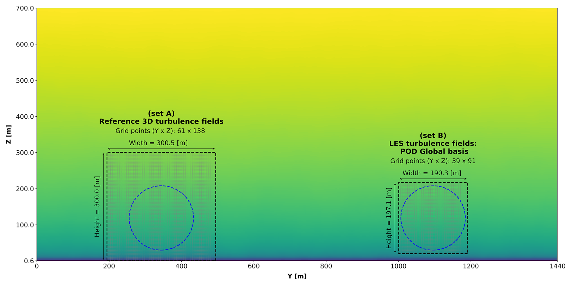
Figure A1 LES wind speed profile representation and the two datasets used in this study, where set A represents the dataset from where the 3D turbulence fields were extracted, while set B represents the location where the dataset for the global POD mode generation was extracted.

Appendix B: Global POD modes

The global POD modes are derived from the inflow database detailed in Sect. 2.3. The first 10 POD modes for the global basis are shown in Fig. B1. These modes are ranked by decreasing total kinetic energy (TKE), revealing large-scale structures in the lower-order modes that progressively diminish in size with increasing mode number. Overall, the resulting spatial modes are consistent with those previously reported for both single-wake scenarios (Sørensen et al., 2015; Bastine et al., 2018) and multiple-wake configurations (Andersen et al., 2013; Andersen and Murcia Leon, 2022).

This consistency highlights the similarity of dominant coherent structures across cases, demonstrating the potential for a reduced-order model built upon these generic patterns (Céspedes Moreno et al., 2025). However, the importance (order) of different modes will differ across different cases, where the low-frequency fluctuations are predominant, and they disappear at higher modes (Andersen and Murcia Leon, 2022).

It is important to note that these POD modes include only the longitudinal (u) fluctuating velocity component, since this is the reconstruction target in our study.

Figure B1 First 10 global POD modes, only estimated for the u component.

Appendix C: Time series

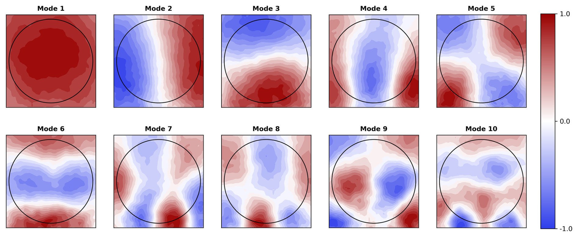
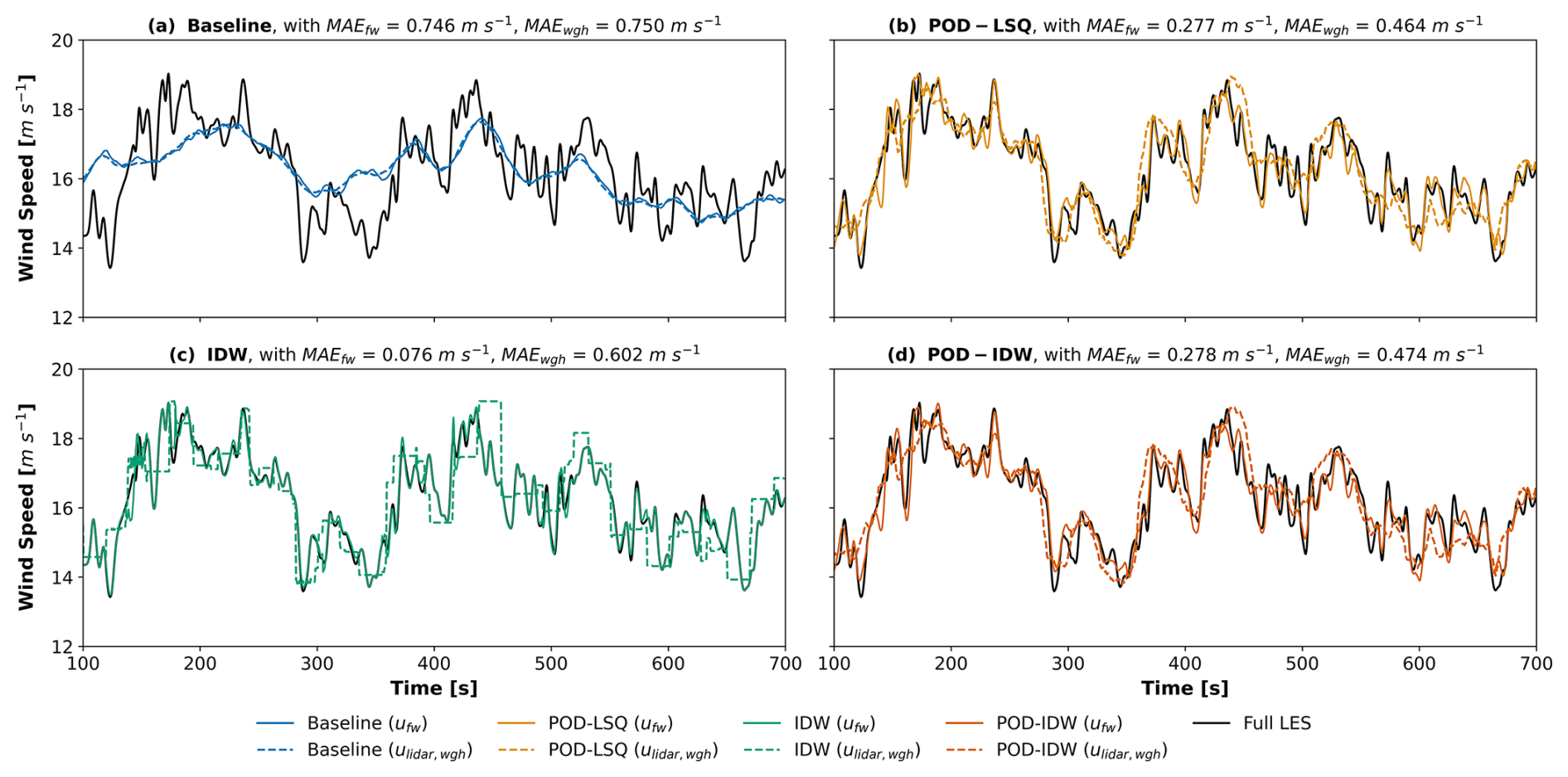
Figure C1 Comparison of 10 min time series for each method at a single location in $y=-\mathrm{65.1}\mathrm{m},z=\mathrm{156.1}\mathrm{m}$, using n_scan=16, θ=22.5°, and K=100 global POD modes for POD-based methods as input parameters for the reconstruction, for the true wind speed (u_fw) and volume-averaged lidar estimate (u_{lidar, wgh}) cases.

To illustrate the effect of increasing the number of scans on the different reconstruction methods, Fig. C1 presents time series at a single location in the YZ plane for all evaluated methods, located at $y=-\mathrm{65.1}\mathrm{m}$ and z=156.1 m (approximate 75 % radius span). Two input cases are considered: the true wind speed (u_fw, solid lines) and the volume-averaged lidar estimate (u_{lidar, wgh}, dashed lines), both using a high scan count of n_scan=16. This high scan count is chosen to highlight the impact of longitudinal spatial filtering, not as a practical recommendation. Above each subplot, the corresponding MAE is reported, representing the time-averaged deviation of the reconstructed signal from the LES reference signal over the full 10 min period.

The baseline method exhibits minimal differences between the two wind speed inputs, effectively capturing the average behavior of the time series but failing to reproduce high-frequency fluctuations. This limitation reflects the method's lack of spatial and temporal adaptability. In contrast, the POD-LSQ method closely follows the LES reference in both amplitude and phase when using the true wind speed (u_fw). However, when using the lidar-based input (u_{lidar, wgh}), it captures the high-frequency variations less accurately. This is caused by the high scan number, which results in a large longitudinal span of the lidar measurements used to fit the POD amplitudes, introducing a low-pass-filtering effect in the time domain. In addition, the inherent probe volume averaging of the lidar further attenuates high-frequency fluctuations (Peña et al., 2017).

The IDW method shows excellent agreement with the LES signal when using u_fw, nearly replicating the full temporal dynamics. Yet, with lidar-based input, its performance declines significantly, yielding blocky and discontinuous reconstructions that highlight its sensitivity to multi-distance fixed-plane mapping error. This is because the IDW method with u_fw samples the true wind at the desired YZ positions in the X_target plane, whereas the values of u_{lidar, wgh} used for interpolation are located at different longitudinal positions. Furthermore, the values for u_fw used during the IDW interpolation are updated at every time step of the simulation, whereas the values for u_{lidar, wgh} do not change. Thus, the time series for IDW with u_{lidar, wgh} has a “quantized” look because the point in space is being interpolated from the same measurement points until enough time has elapsed that a new, closer measurement has been acquired.

While POD-IDW performs slightly worse than POD-LSQ in terms of absolute error, it shows significantly improved robustness compared to IDW when using lidar-based inputs. By applying POD fitting on top of the interpolated IDW field, the method mitigates the blocky and discontinuous behavior introduced by direct IDW interpolation – particularly the “quantized” appearance caused by fixed measurement locations over time. This improvement stems from the projection of the IDW field onto a set of spatial patterns derived from POD, which enforces spatial coherence and smooths out interpolation artifacts. As a result, POD-IDW produces more continuous and physically consistent time series, as further illustrated in Fig. C1d.

Appendix D: Parameter sensitivity of the reconstruction methods

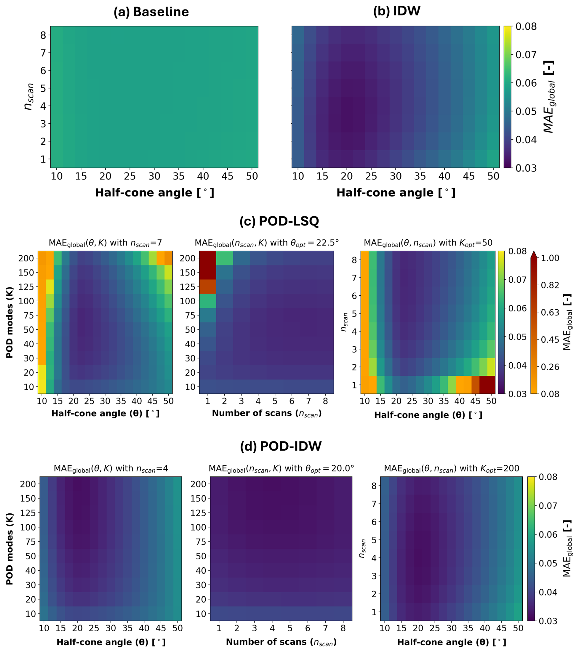
Figure D1 Heat maps of MAE_global, illustrating parameter sensitivity for (a) baseline, (b) IDW, (c) POD-LSQ, and (d) POD-IDW. Baseline and IDW are shown vs. θ and n_scan; the POD-based methods vary two parameters (θ, n_scan, or K) while holding the third fixed (panel titles). A common color scale is used across all panels. POD-LSQ has a second color bar indicating the cases that go beyond the common shared color bar. Adapted from Soto Sagredo (2026).

Figure D1 summarizes the parameter sensitivity of each reconstruction method using heat maps of the global mean absolute error, MAE_global. Panels (a) and (b) show baseline and IDW as functions of the half-cone angle θ and the number of scans n_scan. For POD-LSQ (c) and POD-IDW (d), three parameters are involved (θ, n_scan, and the number of retained POD modes K); therefore, two parameters are varied at a time while the third is fixed at its method-specific optimum (see panel titles). A common color scale is used across all panels to enable direct comparisons, with darker colors indicating lower errors. For POD-LSQ, an additional color bar highlights cases exceeding the shared upper limit, MAE_global=0.08.

The baseline method is largely insensitive to θ and n_scan, with MAE_global increasing only slightly for θ<15°. This behavior is expected because the baseline reduces the inflow to a rotor-equivalent wind speed combined with a prescribed shear profile; changes in spatial sampling or increased cross-contamination therefore have limited impact on the reconstruction. In contrast, IDW (Fig. D1b) shows a moderate dependence on both θ and n_scan. The lowest errors occur for intermediate half-cone angles ($\mathrm{17.5}\mathit{°}<\mathit{\theta }<\mathrm{25.0}\mathit{°}$) and a moderate number of scans, which together improve rotor plane coverage while maintaining an intermediate longitudinal filtering length. Overall, MAE_global varies more strongly with θ than with n_scan, with the largest errors occurring at θ=50.0° and n_scan=1.

POD-LSQ (Fig. D1c) is the most sensitive method, with the strongest dependence on the half-cone angle. Sensitivity increases at high mode counts because accurate reconstruction requires enough measurements per estimate, n_meas≥K, as discussed in Sect. 3.3. When this condition is not satisfied, the least-squares system becomes underdetermined, and accuracy deteriorates substantially (e.g., Fig. 9c for θ=50.0°). This behavior is reflected by the orange-red regions, which denote cases beyond the shared color-scale limit (MAE_global>0.08) and thus indicate pronounced performance loss. For intermediate half-cone angles ($\mathrm{20.0}\mathit{°}<\mathit{\theta }<\mathrm{27.5}\mathit{°}$) and scan counts n_scan≥3, POD-LSQ performs well and benefits from moderate mode truncation (K≈50).

POD-IDW (Fig. D1d) largely follows the trends observed for IDW and thus retains both its advantages and its limitations with respect to parameter selection. Low errors persist across a broad region of intermediate θ and n_scan, particularly for larger mode counts (K>50). In this region, MAE_global varies more strongly with θ than with n_scan. This indicates that POD-IDW is robust to reduced measurement availability and/or degraded spatial coverage, in contrast to POD-LSQ. POD-IDW achieves its lowest errors at high mode counts (here up to K=200) because the POD coefficients are fitted to an IDW-reconstructed rotor plane field rather than directly to sparse measurements, thereby avoiding the underdetermined least-squares problem that constrains POD-LSQ. However, beyond K≈50, further increases in K yield only marginal improvements in accuracy.

Overall, all three spatial reconstruction methods can markedly outperform the baseline when key parameters are selected within appropriate ranges. POD-LSQ is the most sensitive method, with accuracy strongly constrained by measurement availability and rotor plane coverage. By contrast, IDW and POD-IDW provide consistently good performance and greater robustness; POD-IDW attains the lowest errors and is more tolerant than POD–LSQ to variations in half-cone angle and measurement selection.