Field comparison of load-based wind turbine wake tracking with a scanning lidar reference

Wind farm control concepts require awareness and observation methods of the inner-farm flow field. The relative location of the wake, to which a downstream turbine is exposed, is of great interest. It can be used as feedback to support closed-loop wake-steering control, ultimately leading to higher power extraction and fatigue load reduction. With increasing fidelity, not only time-averaged wakes but also instantaneous wake conditions, subject to meandering and wind direction changes, are considered within a controller. This paper presents a quantitative field comparison of two independently applied wake centre estimation methods: a scanning lidar and an extended Kalman filter (EKF) based on the rotor loads of the waked turbine. No ground truth is available in the field environment, therefore the methodology accounts for the fact that two uncertain estimates are compared. The lidar estimates, with a derived uncertainty in the order of 0.05 rotor diameters D, can be used as a suitably precise reference to draw conclusions about the load-based EKF. The EKF uses Coleman-transformed blade root bending moments, linked to the wake centre position via an analytical model with a low number of tuning parameters. The model can easily be trained with aeroelastic simulations, including the dynamic wake meandering model. The formulation adds robustness to the tracking and allows the user to determine the confidence in the wake position estimate, which can be used for wake impingement detection or for a wake-steering controller to judge whether a yaw manoeuvre is adequate. The results indicate agreement of the methods with root mean square errors of 0.2D for low and moderate turbulence intensity, and 0.3D for turbulence intensities above 12 %. The paper focuses on wake position estimation but also outlines a methodology for validating wind farm models and wind field reconstruction techniques with complementary lidar data.

1 Introduction

Wind farm flow control allows the user to partly compensate wake-induced power losses or load increases. Wake steering, static induction control, or wake mixing strategies are employed to that purpose (Meyers et al., 2022). So far, mostly open-loop approaches are considered for wake steering, namely misaligning or dynamically actuating the upstream turbine(s) without considering feedback of the wake-exposed turbines (see e.g. Fleming et al., 2017; Doekemeijer et al., 2021). Here, the yaw controller relies on engineering models for the wake trajectory it tries to aim for. While robust formulations can account for wind direction variability (Rott et al., 2018; Simley et al., 2020), optimal wake deflection cannot be guaranteed, since outer influences and wake dynamics can hardly be accounted for. The wake trajectory is impacted by atmospheric stability and further subject to the meandering motion (Larsen et al., 2015; Sengers et al., 2023).

The consequent next step is to close the loop by providing suitable feedback signals to a wind farm controller. Meyers et al. (2022) explicitly mention the need for state estimation on the wind farm level, i.e. for the awareness of the flow conditions within the farm. Standard SCADA data and basic instrumentation of modern wind turbines, for example strain gauges for blade root bending moments, allow the rotor to be used as a sensor. Rotor-effective measurements such as power, torque, and collective blade loads provide observability towards rotor-effective wind speeds (Soltani et al., 2013; Bottasso et al., 2018; Lio et al., 2023; Coquelet et al., 2024). This can be used as direct feedback or to tune an analytical flow model, as shown by Doekemeijer and van Wingerden (2020) and Becker et al. (2022). Yet, the observability is limited, as shown for example by Doekemeijer and van Wingerden (2020), where the estimator can hardly distinguish which half of the rotor is exposed to a partial wake, especially under uncertain wind direction information. In order to increase the spatial observability of non-uniform turbine inflow, the rotor imbalances – resulting from shear, yaw misalignment, or wake impingement – can be encountered (Bertelè et al., 2017). These rotor imbalances, such as yaw and tilt moments, are related to the harmonics of the blade root bending moments. The Coleman transform describes the translation from the rotating to the non-rotating coordinate system.

Ultimately relevant for wake-steering control is the wake position within the wind farm, which is the feature that a wind farm controller aims to manipulate. Existing methods for the wake position estimation are based either on wind turbine rotor loads or the light detection and ranging (lidar) measurements. The load-based approaches described by Bottasso et al. (2018) and Schreiber et al. (2020) aim at qualitative impingement detection and include a field validation. Time-averaged position tracking is shown by Cacciola et al. (2016) in aeroelastic simulations and by Schreiber et al. (2016) in a wind tunnel.

Yet, the dynamics caused by wind direction changes and wake meandering are not taken into account here. Braunbehrens et al. (2023) show that these dynamic scales are relevant for the inner-farm flow but are also challenging for an estimator to capture. As outlined by Larsen et al. (2008) and further described in Sect. 2.2.2, the spatial scales in the order of 2–20 rotor diameters (or their complementary time scales) need to be considered in the context of wake meandering. Dynamic EKF formulations are shown by Dong et al. (2021) and Onnen et al. (2022), using blade loads but also taking the meandering dynamics into account. Yet, these methods are only tested in simulation environments, where the wake position is known.

The lidar-based wake-tracking methodologies depend on the lidar type. The online approaches for wind farm control purposes use short-range forward-looking lidars, usually considering a low number of fixed beams for cost efficiency (Raach et al., 2017; Lio et al., 2021). Kalman filter formulations are used for robustness under the sparse spatial observability owing to the low number of beams. They are similar to the load-based attempts but can further include the wake deficit shape to the estimation Lio et al. (2021). In contrast, long-range scanning lidars provide a high spatial resolution of the flow field. Due to their high costs, they are not considered for commercial applications in the context of real-time wind farm flow control. Instead, they are mainly used in experimental campaigns for the scientific validation of wake behaviour (Trujillo et al., 2011; Machefaux et al., 2015; Bromm et al., 2018; Brugger et al., 2022). Both wake steering (Bromm et al., 2018) and wake meandering (Brugger et al., 2022) effects can be resolved.

In Sect. 4.2.2, the results of the load- and lidar-based wake estimation approaches mentioned above are compared to the approach presented in this paper, considering the individual testing conditions and performance metrics. At this point, the research gap can be concluded as follows: existing work for load-based wake tracking lacks

• a consideration of wake dynamics and time resolution, or

• a field validation, or

• (in the case of a field validation) an independent reference to compare with.

The objective of this work is to fill the gap by addressing all three aspects: the work shows the direct estimation of the instantaneous wake centre position in a field experiment with two utility-scale wind turbines. The load-based estimate is compared to the wake position probed with a scanning lidar, which serves as an independent reference. To that purpose, the uncertainty of the lidar estimate is quantified using analytic error propagation following the GUM (Guide to the expression of uncertainty in measurement; JCGM, 2020). The lidar data processing orients at existing work of Machefaux et al. (2015) and Bromm et al. (2018), isolating the quasi-instantaneous wake deficit in a moving frame of reference.

The remainder of the paper is structured as follows: in Sect. 2, the methodology is described, starting with the field setup, followed by the load-based EKF and the lidar-related data processing, including an uncertainty consideration. In Sect. 3, the results are presented. First, the experimental conditions are characterized, and then the wake position estimates are compared. In Sect. 4, the findings are discussed, ranged, and compared with literature. Concluding remarks are given in Sect. 5.

2 Methodology

2.1 Field experiment

The wind farm used in this work consists of two Eno126 turbines, built by Eno Energy Systems GmbH near the village of Kirch Mulsow near Rostock, Germany, close to the Baltic Sea. The surrounding nature of the test site has agricultural vegetation, with patches of trees and bushes between the fields. The measurements used for this paper are from February and March 2021. Further investigations of the experiments at this site are reported in Hulsman et al. (2022), Sengers et al. (2023), and Kidambi Sekar et al. (2024). The turbines are spaced by 2.7 rotor diameters along a south-westerly direction (compare Fig. 1), which is also the prevailing wind direction for this site. For brevity, the turbines are called WT1 and WT2 in the following, with WT1 located in the south-west, thus mostly being the upstream turbine. Each turbine has a rotor diameter D of 126 m and a rated power of 3.5 MW. The hub heights are 117 and 137 m for WT1 and WT2, respectively. In addition to standard operational signals, both turbines are equipped to measure blade root bending moments in flapwise and edgewise directions with strain gauges and fibre-optical sensors. This paper uses the fibre-optical sensors by Polytech Wind Power Technology Germany GmbH (formerly Fos4X GmbH). Both turbines' nacelle yaw orientation is tracked with interconnected differential Global Navigation Satellite System (GNSS) devices (Trimble type 3 Zephyr mode, three antennas on WT1 and two on WT2l; see Trimble, 2025). The increased accuracy of the yaw angle probing in comparison to the inbuilt yaw encoders is relevant for the post-processing of the lidar measurements, as recommended by Bromm et al. (2018). The rotor azimuth angle information of WT2 was not available, thus the angle was reconstructed from the gravity-dominated edgewise blade loads, as shown in Appendix A.

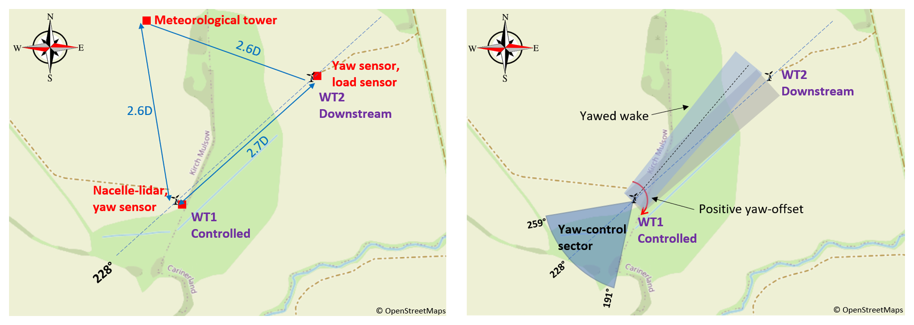
Figure 1 Wind farm layout at the Kirch Mulsow test site. Left: turbine spacing and distance to the met mast indicated; right: wind sectors for the control experiment indicated; adapted from Hulsman et al. (2022). © OpenStreetMap contributors 2024 (https://www.openstreetmap.org/copyright). Distributed under the Open Data Commons Open Database License (ODbL) v1.0.

A met mast is located 2.6D north of WT1 (see Fig. 1). The wind speed and direction are probed with cup anemometers and vanes (Thies-Clima, type 4.3352.00.400 (Thies-Clima, 2025b) and type 4.3151.00.212 (Thies-Clima, 2025a), respectively) at z₁=54 m and z₂=112 m. Both the turbine and met the mast data are stored at 50 Hz.

The wind shear exponent α is calculated from the met mast measurements according to the power law:

$$\begin{array}{}\text{(1)}& \mathit{\alpha }={\displaystyle \frac{\log (u_{\mathrm{2}}/u_{\mathrm{1}})}{\log (z_{\mathrm{2}}/z_{\mathrm{1}})}},\end{array}$$

where u_i, $i\in \mathrm{1},\mathrm{2}$ is the wind speed and z_i, $i\in \mathrm{1},\mathrm{2}$ is the height of the wind cup anemometers.

A pulsed scanning lidar (Leosphere WindCube 200S) is installed on the nacelle of WT1, facing in a downstream direction. Within the wind direction sector under investigation, the lidar performs horizontal trajectories (single plan position indicator, or PPI). The scanned sector covers a range of 120° with a scanning speed of 2° s⁻¹ and range gates between 50 and 1630 m. The coordinate systems involved in the post-processing and further details on the lidar trajectory are described in Sect. 2.3.1.

Within the wind direction interval [191°,259°], active wake steering control is tested. At intervals of 30 min, the controller of WT1 toggles between greedy and intentional yaw misalignment. The yaw update frequency is at 30 s, and the misalignment is realized via the manipulation of the nacelle vane signal. The assessment of the wake steering controller is not the focus of this paper, yet it is important to regard its role when discussing the wake constellations.

2.2 Load-based wake tracking

In this section, the methods used for the load-based wake tracking algorithm and usage of training data are described. Core of the tracking algorithm is an extended Kalman filter (EKF), which links the load measurements from a wake-exposed wind turbine with the physical knowledge about the wake dynamics. An EKF incorporates non-linear state- and measurement transition functions via local linearization around the current state estimate (Brown and Hwang, 1992). The interaction between the individual aspects of the load-based wake tracking problem is shown in the overview chart in Fig. 2. The EKF and its sub-components are described in the following sections. In Sect. 2.2.1, the EKF formulation and the definition of states and inputs takes place. Section 2.2.2 defines the state transition function f(), including a consideration of the involved wake physics. Section 2.2.3 defines the measurement transition function h(), i.e. the linkage between wake position and rotor loads.

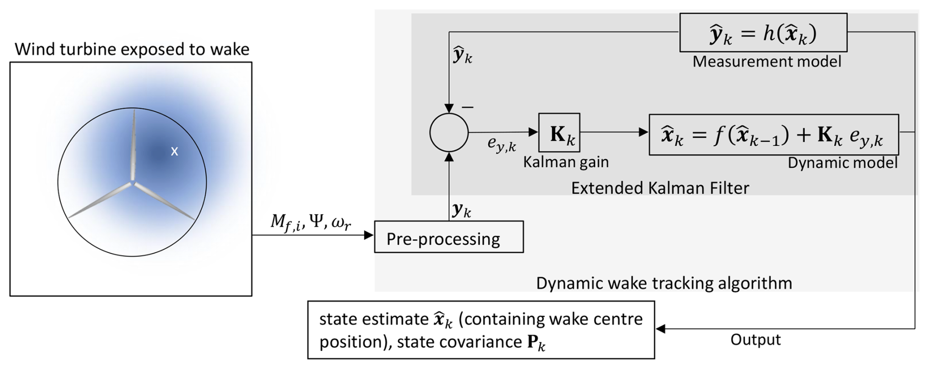
Figure 2 Block diagram of the dynamic wake tracking algorithm, showing the input and output signals to the EKF.

Note that the estimation task is here formulated for the general two-dimensional case, which considers the horizontal and vertical wake position. Due to the measurement setup and the single PPI scans of the lidar, only a comparison of the horizontal component is possible, which is also more relevant. The vertical position is considered less relevant for the application, because (i) it has lower position variance due to wind direction changes and meandering (Braunbehrens and Segalini, 2019), and (ii) it cannot be manipulated by wake-steering control.

2.2.1 General EKF setup

A discrete EKF is implemented, where k denotes the time index, $\widehat{(\cdot )}$ an estimate, ${\mathit{x}}_k\in {\mathbb{R}}^{N_x}$ the state vector, and ${\mathit{y}}_k\in {\mathbb{R}}^{N_y}$ the measurement vector, with dimensions N_x=4 and N_y=3. The state vector contains the wake positions (y_w,z_w) in a WT2-oriented coordinate system (compare Sect. 2.3.1), as well as their first derivatives with time (v_c,w_c). The measurement vector y_k contains the Coleman-transformed non-rotating rotor loads, further described in subsection 2.2.3.

$$\begin{array}{}\text{(2)}& {\mathit{x}}_k=[y_{\mathrm{w}},z_{\mathrm{w}},v_{\mathrm{c}},w_{\mathrm{c}}{]}^T,{\mathit{y}}_k=[M_{\mathrm{yaw}},M_{\mathrm{tilt}},M_{\mathrm{col}}{]}^T\end{array}$$

The EKF algorithm consists of the steps presented in Eqs. (3)–(7). An a priori value is denoted as $(\cdot {)}^{-}$. The model ${\mathit{x}}_{k+\mathrm{1}}=f({\mathit{x}}_k,{\mathit{n}}_{x,k})$ describes the state transition, and the measurement model ${\mathit{y}}_k=h({\mathit{x}}_k,{\mathit{n}}_{y,k})$ describes the static mapping between the system state and measurements, where ${\mathit{n}}_{x,k}\in {\mathbb{R}}^{N_x}$ and ${\mathit{n}}_{y,k}\in {\mathbb{R}}^{N_y}$ represent white noise acting on the state and output equation, respectively, with zero mean and covariance matrices Q and R. The state covariance matrix is denoted as P_k. It is initialized as ${\mathbf{P}}_{k=\mathrm{0}}=\mathbf{Q}$. The local linearizations of the state transition model and the measurement model around a current state are denoted as F_k and H_k, respectively. Note that the state transition model $f({\mathit{x}}_k,{\mathit{n}}_{x,k})$ used in this work is formulated as a linear operation (see next subsection). Thus, the linearization in Eq. (4) is not necessary and F can be directly constructed from Eq. (8a)–(8d). In the scope of this work, the EKF is applied at 1 Hz sampling frequency.

Prediction step:

$$\begin{array}{}\text{(3)}& {\displaystyle }{\widehat{\mathit{x}}}_k^{-}=f({\widehat{\mathit{x}}}_{k-\mathrm{1}},\mathrm{0})\text{(4)}& {\displaystyle }{\mathbf{P}}_k^{-}={\mathbf{F}}_k{\mathbf{P}}_{k-\mathrm{1}}{\mathbf{F}}_k^T+\mathbf{Q}\mathrm{with}{\mathbf{F}}_k={\displaystyle \frac{\partial f({\mathit{x}}_{k-\mathrm{1}},\mathrm{0})}{\partial \mathit{x}}}.\end{array}$$

Measurement update step:

$$\begin{array}{}\text{(5)}& {\mathbf{K}}_k={\mathbf{P}}_k^{-}{\mathbf{H}}_k^T({\mathbf{H}}_k{\mathbf{P}}_k^{-}{\mathbf{H}}_k^T+\mathbf{R}{)}^{-\mathrm{1}}\mathrm{with}{\mathbf{H}}_k={\displaystyle \frac{\partial h({\mathit{x}}_k^{-},\mathrm{0})}{\partial \mathit{x}}}\end{array}$$

$$\begin{array}{}\text{(6)}& {\displaystyle }{\widehat{\mathit{x}}}_k={\widehat{\mathit{x}}}_k^{-}+{\mathbf{K}}_k\underset{\mathrm{innovation}{e}_{y,k}}{\underbrace{({\mathit{y}}_k-{\widehat{\mathit{y}}}_k)}}\mathrm{with}{\widehat{\mathit{y}}}_k=h({\widehat{\mathit{x}}}_k^{-},\mathrm{0})\text{(7)}& {\displaystyle }{\mathbf{P}}_k=(\mathbf{I}-{\mathbf{K}}_k{\mathbf{H}}_k){\mathbf{P}}_k^{-}.\end{array}$$

2.2.2 Dynamic model

The dynamic model f() describes how the system state evolves over time. In this study, the model should capture how the wake centre position changes over time. Depending on the atmospheric conditions and the wind farm control strategy, the wake trajectory is subject to various dynamic influences. Time scales of wind direction changes, wake-steering control and wake meandering need to be incorporated by the dynamic model of the EKF, while the effects corresponding to small-scale turbulence with no expressiveness towards the wake position need to be rejected.

For the inner-farm effect of wind direction variability, Simley et al. (2020) suggest a distinction between low- and high-frequency wind direction. The high-frequency share refers to oscillatory point-measurements (e.g. a nacelle vane) at the hub height of a wind turbine, while the low-frequency share describes the dominant mean wind direction across the wind farm. Using a combination of field measurements and large-eddy simulations (LESs), Simley et al. (2020) identify the boundary between high- and low-frequency wind direction at 0.0037 Hz for a scenario at 8 m s⁻¹ ambient wind speed and wind turbines of 126 m rotor diameter (NREL 5 MW). Rott et al. (2018) suggest to regard a time window of 5 min ($\widehat{=}$ 0.0033 Hz), which is very similar. Using the same non-dimensional type of expression as in Larsen et al. (2008) and Lio et al. (2021), this frequency can be expressed as $f_{\mathrm{c},\mathrm{WD}}\approx u_{\mathrm{\infty }}/\left(\mathrm{20}D\right)$, where u_∞ is the ambient undisturbed mean wind speed. Depending on the perspective, a high-frequency wind direction variation can also be seen as the vector addition of longitudinal and transversal wind speed components, i.e. a turbulence phenomenon.

Wake meandering in the atmospheric boundary layer is driven by turbulence patterns considerably larger than the wake deficit scale (Trujillo et al., 2011). Larsen et al. (2008) introduced the dynamic wake meandering (DWM) model, which translates this split of scales to a random walk trajectory, where the wake deficit is seen as a passive tracer. Larsen et al. (2008) and Larsen and Lio (2025) define the default cut-off frequency of the meandering motion as $f_{\mathrm{c}}=u_{\mathrm{\infty }}/\left(\mathrm{2}{D}_{\mathrm{w}}\right)$, where D_w is the wake diameter (in near-wake applications, the rotor diameter D is also a valid choice). Note that this is the theoretical limit, up to which a wake deficit is regarded as a passive tracer. Lio et al. (2021) show in a field study with a lidar-based EKF featuring an auto-correlation term of the wake position time history that the dominant spectral share of the meandering motions can be up to a factor 10 slower.

In conclusion, the frequency range of $\frac{u_{\mathrm{\infty }}}{\mathrm{20}D}\le f\le \frac{u_{\mathrm{\infty }}}{\mathrm{2}D}$ is relevant for meandering. Wake position changes at slower time scales do not require a higher-order model. The meandering time scales are thus modelled with 1st-order differential equations. This work uses a cut-off frequency of f_c=0.01 Hz. The changes in lateral and vertical wake position are described via the characteristic velocities v_c(t) and w_c(t), whose change rates are modelled as low-pass-filtered white noise:

$$\begin{array}{}\text{(8a)}& {\displaystyle }{\dot{y}}_{\mathrm{w}}\left(t\right)=v_{\mathrm{c}}\left(t\right)+n_{x,\mathrm{1}}\left(t\right)\text{(8b)}& {\displaystyle }{\dot{z}}_{\mathrm{w}}\left(t\right)=w_{\mathrm{c}}\left(t\right)+n_{x,\mathrm{2}}\left(t\right)\text{(8c)}& {\displaystyle }{\dot{v}}_{\mathrm{c}}\left(t\right)=-{\mathit{\omega }}_{\mathrm{c}}{v}_{\mathrm{c}}\left(t\right)+{\mathit{\omega }}_{\mathrm{c}}{n}_{x,\mathrm{3}}\left(t\right)\text{(8d)}& {\displaystyle }{\dot{w}}_{\mathrm{c}}\left(t\right)=-{\mathit{\omega }}_{\mathrm{c}}{w}_{\mathrm{c}}\left(t\right)+{\mathit{\omega }}_{\mathrm{c}}{n}_{x,\mathrm{4}}\left(t\right),\end{array}$$

where ω_c=2πf_c. The equations are discretized for their implementation in the state transition function $f({\mathit{x}}_k,{\mathit{n}}_{x,k})$. Note that the n_x,i represents the ith element of the noise vector n_x. The time index k is omitted here, because the continuous representation is chosen. Since the noise terms enter linearly, they are incorporated in the EKF formulation via the additive noise covariance matrix Q.

2.2.3 Measurement model

The measurement model h() is a mapping from the state to the measurement – in this study, a link from the wake centre position to the rotor loads. The model must fulfil certain criteria: it should be computationally inexpensive, such that it can be computed online in each filter iteration. Look-up tables with pre-computed information are preferable here (see e.g. Schreiber et al., 2020; Soltani et al., 2013). Moreover, the model has to be differentiable, such that its local sensitivity to a change in state or input can be determined. Finally, it should be robust and lead to a convergence of the estimate, even if the state at initialization is far off. The measurement vector y_k contains the Coleman-transformed, non-rotating flapwise blade root bending moments according to Eq. (9). The time index k is omitted from the notation for better readability.

$$\begin{array}{}\text{(9)}& \begin{array}{rl}\mathit{y}& =\left[\begin{array}{c}{M}_{\mathrm{yaw}}\\ M_{\mathrm{tilt}}\\ M_{\mathrm{col}}\end{array}\right]+{\mathit{n}}_y\\ & ={\displaystyle \frac{\mathrm{2}}{\mathrm{3}}}\left[\begin{array}{ccc}\sin \left(\mathrm{\Psi }\right)& \sin (\mathrm{\Psi }+\frac{\mathrm{2}\mathit{\pi }}{\mathrm{3}})& \sin (\mathrm{\Psi }+\frac{\mathrm{4}\mathit{\pi }}{\mathrm{3}})\\ \cos \left(\mathrm{\Psi }\right)& \cos (\mathrm{\Psi }+\frac{\mathrm{2}\mathit{\pi }}{\mathrm{3}})& \cos (\mathrm{\Psi }+\frac{\mathrm{4}\mathit{\pi }}{\mathrm{3}})\\ \mathrm{1}/\mathrm{2}& \mathrm{1}/\mathrm{2}& \mathrm{1}/\mathrm{2}\end{array}\right]\left[\begin{array}{c}{M}_{\mathrm{f},\mathrm{1}}\\ M_{\mathrm{f},\mathrm{2}}\\ M_{\mathrm{f},\mathrm{3}}\end{array}\right]+{\mathit{n}}_y,\end{array}\end{array}$$

where Ψ denotes the rotor azimuth position and M_f,i denotes the ith blade flapwise blade root bending moment.

Table 1 Fitting parameter for the measurement model h().

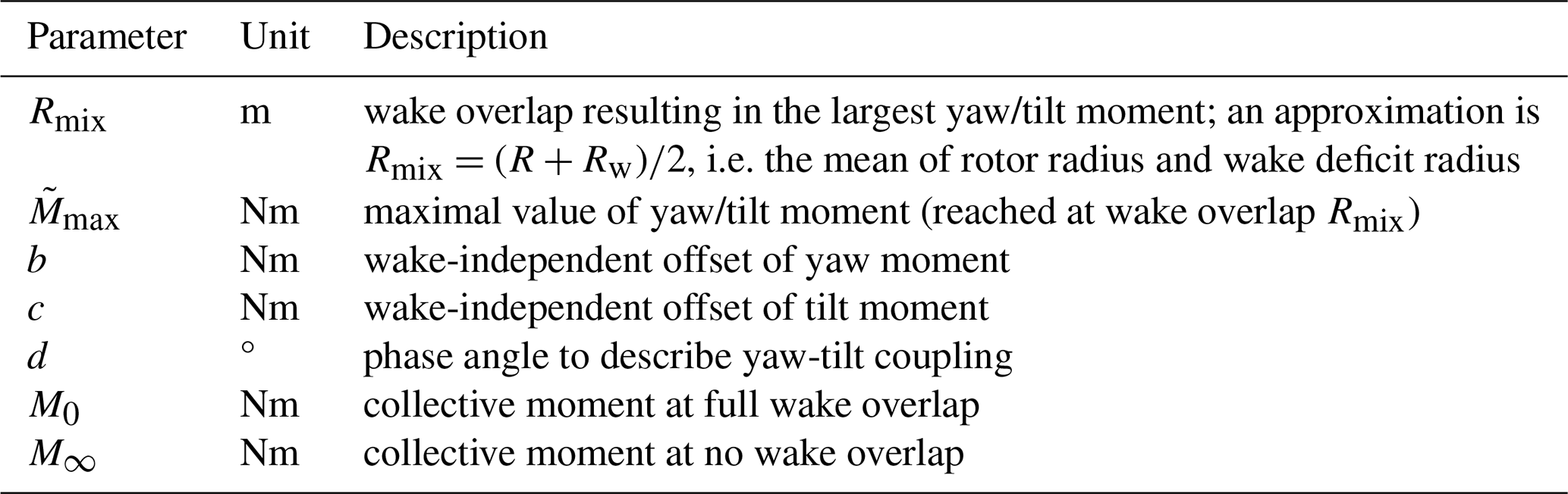
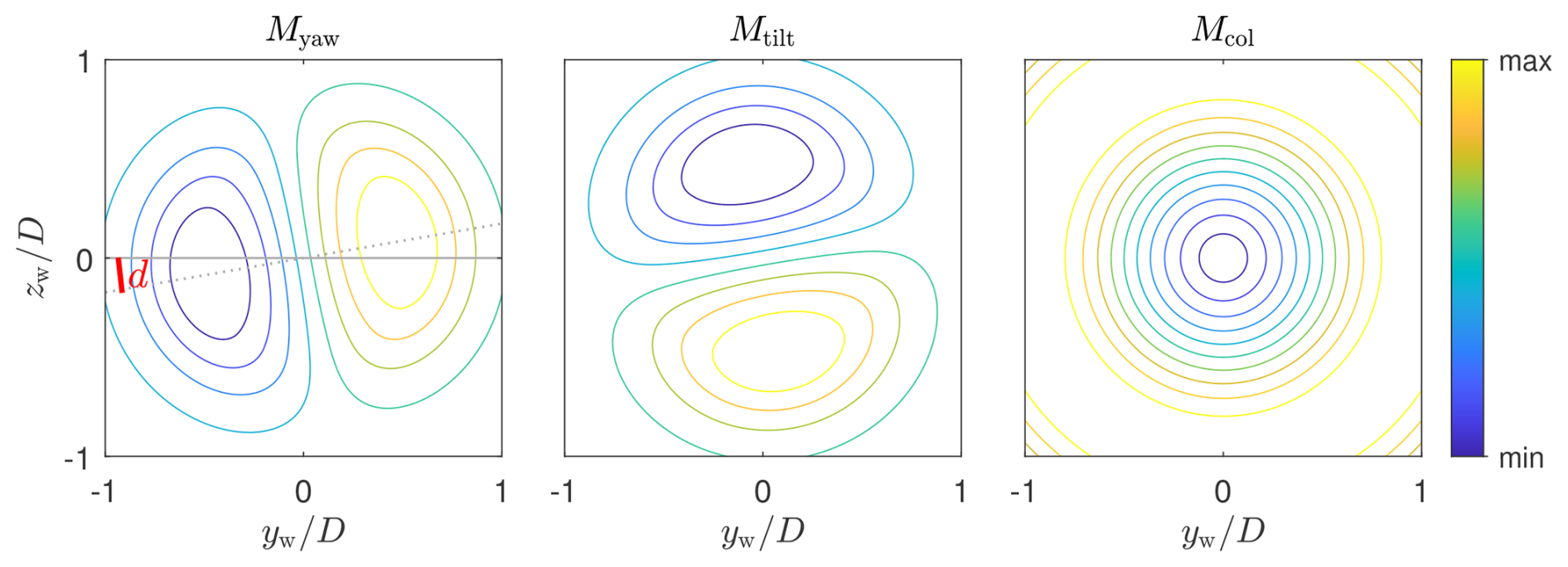
Figure 3 Contour plot of the measurement model outputs in dependency of the wake position, normalized with their respective maximum and minimum for confidentiality. The fitting parameter d is indicated, describing the phase offset of the yaw-tilt coupling.

In the following, the parameterized model is derived in Eqs. (10)–(13). All fitting parameters introduced in this scope are listed in Table 1. The model is subsequently fitted to training data generated in aeroelastic simulations with the enabled DWM model (Larsen et al., 2008). Figure 3 shows the contour shape of the model, and Fig. 4 is an example of training data and fitting.

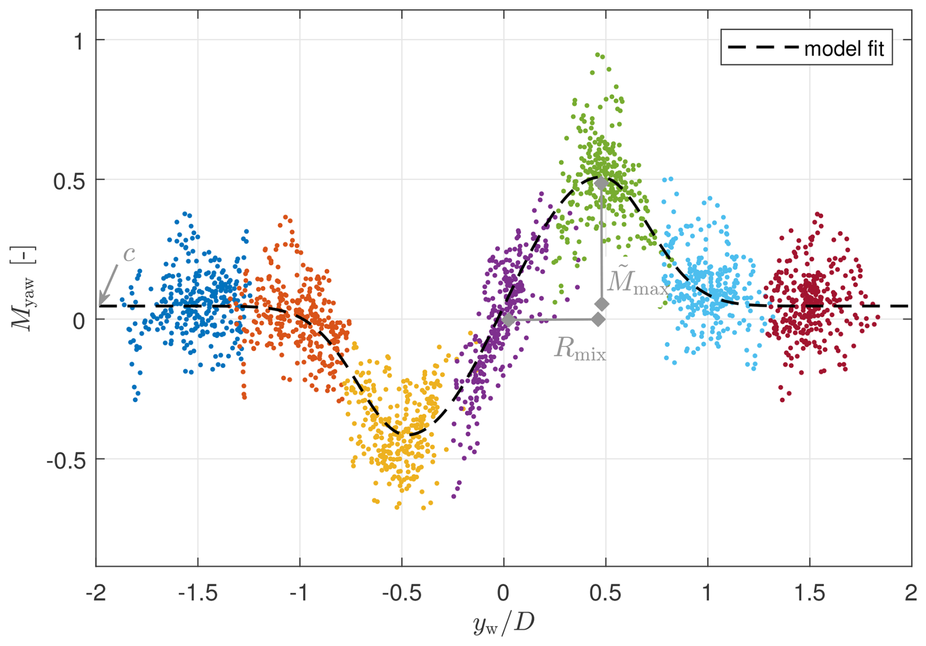
Figure 4 Training data and model fit of the yaw moment; each scatter colour refers to a prescribed position of WT1, normalized with the respective maximum and minimum for confidentiality. The fitting parameter R_mix, ${\stackrel{\mathrm{̃}}{M}}_{\max }$, and c are indicated, showing the width, amplitude, and offset of the model, respectively.

The yaw and tilt moment depend on the wake position (y_w,z_w) relative to the rotor. Let these be expressed in polar coordinates centred at the hub, where $r_{\mathrm{w}}=\sqrt{y_{\mathrm{w}}^{\mathrm{2}}+z_{\mathrm{w}}^{\mathrm{2}}}$ is the distance of the hub to the wake centre. The ratio between rotor tilt and yaw moment yields information about the angle θ and the angular position of a wake in the rotor plane, quantified as $\mathit{\theta }=\mathrm{atan}(y_{\mathrm{w}}/z_{\mathrm{w}})$ using a four-quadrant inverse tangent. In order to get the absolute magnitude of the wake-induced rotor imbalance, the quantity $\stackrel{\mathrm{̃}}{M}\left(r_{\mathrm{w}}\right)$ is introduced as

$$\begin{array}{}\text{(10)}& \stackrel{\mathrm{̃}}{M}\left(r_{\mathrm{w}}\right)=\sqrt{{\left(M_{\mathrm{yaw}}(r_{\mathrm{w}},\mathit{\theta })-b\right)}^{\mathrm{2}}+{\left(M_{\mathrm{tilt}}(r_{\mathrm{w}},\mathit{\theta })-c\right)}^{\mathrm{2}}}.\end{array}$$

A reformulation yields the following compact formulation of the yaw and tilt moments

$$\begin{array}{}\text{(11a)}& {\displaystyle }{M}_{\mathrm{yaw}}(r,\mathit{\theta })=\stackrel{\mathrm{̃}}{M}\left(r_{\mathrm{w}}\right)\cdot \sin (\mathit{\theta }+d)+b\text{(11b)}& {\displaystyle }{M}_{\mathrm{tilt}}(r,\mathit{\theta })=\stackrel{\mathrm{̃}}{M}\left(r_{\mathrm{w}}\right)\cdot \cos (\mathit{\theta }+d)+c,\end{array}$$

where b and c describe offsets to the moments that do not originate from the wake, such as a moment due to tilt overhang or vertical shear. An optional term for phase delay is denoted as d, describing how an inert blade reacts to a change of local wind speed, also known as yaw-tilt coupling (see Lu et al., 2015 and Mulders et al., 2019). The quantity $\stackrel{\mathrm{̃}}{M}\left(r_{\mathrm{w}}\right)$ is defined in Eq. (12), where ${\stackrel{\mathrm{̃}}{M}}_{\max }$ and R_mix are fitting constants.

$$\begin{array}{}\text{(12)}& \stackrel{\mathrm{̃}}{M}\left(r_{\mathrm{w}}\right)=\left\{\begin{array}{ll}{\stackrel{\mathrm{̃}}{M}}_{\max }\sin \left(\frac{\mathit{\pi }{r}_{\mathrm{w}}}{\mathrm{2}{R}_{\mathrm{mix}}}\right)& \mathrm{if}\left|r_{\mathrm{w}}\right|<R_{\mathrm{mix}}\\ {\stackrel{\mathrm{̃}}{M}}_{\max }\exp \left(\mathrm{2}{\left(\frac{r_{\mathrm{w}}}{R_{\mathrm{mix}}}-\mathrm{1}\right)}^{\mathrm{2}}\right)& \mathrm{if}\left|r_{\mathrm{w}}\right|\ge R_{\mathrm{mix}}\end{array}\right.\end{array}$$

Although wake tracking based only on rotor imbalance (M_yaw,M_tilt) was found to be possible, the stability and convergence behaviour can be enhanced by including the collective moment M_col (Onnen et al., 2022). The relation between r_w and M_col is linked to the control strategy of the wind turbine and the rotor-effective wind speed (REWS). A larger r_w leads to a higher REWS, until the wake is so far from the rotor centre that no overlap with the rotor takes place and the REWS approaches u_∞. This means that in the partial load region, M_col is suppressed with more wake overlap, i.e. for decreasing r_w. In the full load region, the blades are pitched to keep the power (∝u³) constant, which implies that the thrust and the flapwise moments (∝u²) decrease with increasing wind speed. The highest loading can be seen at rated wind speed. Consequently, M_col increases with more wake overlap in the full load region, down to the point when the REWS becomes smaller than the rated wind speed. M_col is fitted with a Gaussian function of σ=R_mix. The constants M_∞ and M₀ describe the collective moment for r_w→∞ and r_w=0, respectively.

$$\begin{array}{}\text{(13)}& M_{\mathrm{col}}\left(r\right)=M_{\mathrm{\infty }}-(M_{\mathrm{\infty }}-M_{\mathrm{0}})\exp \left(-{\displaystyle \frac{r_{\mathrm{w}}^{\mathrm{2}}}{\mathrm{2}{R}_{\mathrm{mix}}^{\mathrm{2}}}}\right)\end{array}$$

The characteristic shape of the measurement model as described above is illustrated in Fig. 3.

The parameters of the measurement model (see Table 1) are fitted to a set of training data from aeroelastic simulations within the framework of FASTfarm (Branlard et al., 2022) via a non-linear least-squares regression. The field setup is replicated in the simulations, but the position of WT1 is subsequently shifted laterally from −1.5D to +1.5D in steps of 0.5D. The DWM model is enabled, and the curled wake model is chosen (Branlard et al., 2022). As an example, a subset of the training data at 10 m s⁻¹ ambient wind speed is given in Fig. 4, showing the non-dimensionalized yaw moment in dependency of the wake position y_w. Each scatter colour refers to one location of WT1. The combination of wake meandering and different WT1 positions results in a wide range of wake constellations being covered. In the case of a constellation with larger downstream spacing, thus larger meandering amplitudes, even fewer WT1 positions could be considered for the generation of training data.

The fit parameters depend on the ambient conditions, most prominently on the ambient wind speed. Information of the wake deficit is implicitly contained in the parametric model. Especially in the case of large downstream distances, ambient turbulence and atmospheric stability impact the wake mixing. In the present case, however, the streamwise spacing is too short for the ambient turbulence to show a notable impact on the modelled wake mixing and thus on the fitting parameters. The impact of shear on the wake deficit is not fully accounted for in the simulation environment, especially in relation to wake asymmetry (as discussed later in Sect. 4.1). Thus, it is decided to only create training data in dependency of the ambient wind speed, resulting in a one-dimensional lookup-table (LUT) of fitting parameters. This requires 63 simulations (7 WT1 positions and 9 wind speeds, 4–12 m s⁻¹), each with a duration of 600 s, a TI of 10 %, and α=0.25. Only one stochastic seed per wind field proved sufficient, since the set for one ambient condition already combines the results of seven simulations with their respective wind field (referring to the seven lateral WT1 positions). Depending on the scenario, a higher-dimensional LUT can be required. A consideration of ambient TI is required in case of larger streamwise spacing to adequately resolve the impact of turbulent mixing in the far-wake region. Also, including ambient shear could be a further step, preferably with a refined modelling of its impact on the wake deficit.

In addition to parameter fitting, the training data allows insight into the order of magnitude of the load variance, which is linked to turbulence and dynamic events such as load over- and undershoots. This variance is regarded in the noise tuning of the EKF when choosing the entries in the measurement covariance matrix R. The measurement covariance of the yaw moment is increased by a factor of 10 in situations when the turbine is yawing, to prevent a misinterpretation of the yaw moments occurring here.

2.3 Lidar data processing

This section describes the steps from the initial scanning lidar measurements to a wake position in a WT2-based coordinate system. An uncertainty analysis is included to show the eligibility of the lidar measurements as a suitably precise reference.

2.3.1 Coordinate systems

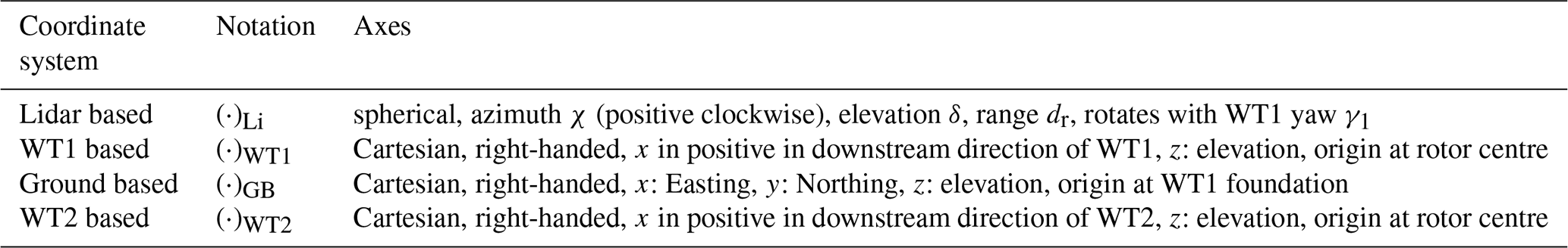
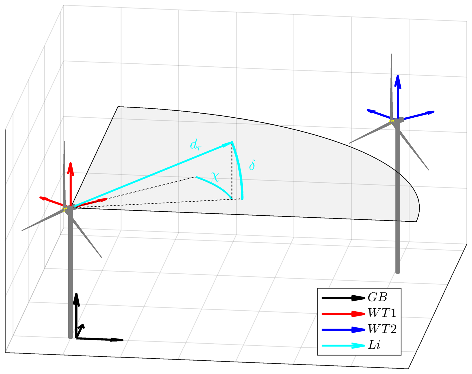
Different coordinate systems occur in the scope of this work. An overview is shown in Table 2. Ultimately, the lidar-probed wake positions should serve as the reference for the load-based tracking of WT2, thus a WT2-centred coordinate system is targeted. The relations between the coordinate systems are given in Eqs. (14)–(16), and an overview is sketched in Fig. 5. The x and y offsets in Eq. (16) refer to the 2.7D spacing in ground-based coordinates. The lidar performs horizontal single PPI scans. An elevation of δ=1.3° is used to account for the average nacelle tilt during operation, determined via the GNSS system on WT1. The lidar azimuth angle χ covers a range of 120° with a scanning speed of 2° s⁻¹. The range gate centre is denoted as d_r and spans from 50 to 1630 m in steps of 10 m. The nacelle yaw angles are denoted as γ₁ and γ₂ for WT1 and WT2, respectively.

$$\begin{array}{}\text{(14)}& {\displaystyle }{\left[\begin{array}{c}x\\ y\\ z\end{array}\right]}_{\mathrm{WT}\mathrm{1}}=d_{\mathrm{r}}{\left[\begin{array}{c}\cos \left(\mathit{\chi }\right)\cos \left(\mathit{\delta }\right)\\ \sin \left(\mathit{\chi }\right)\cos \left(\mathit{\delta }\right)\\ \sin \left(\mathit{\delta }\right)\end{array}\right]}_{\mathrm{Li}}\text{(15)}& {\displaystyle }\begin{array}{rl}{\left[\begin{array}{c}x\\ y\\ z\end{array}\right]}_{\mathrm{GB}}& =\left[\begin{array}{ccc}-\sin \left({\mathit{\gamma }}_{\mathrm{1}}\right)& \cos \left({\mathit{\gamma }}_{\mathrm{1}}\right)& \mathrm{0}\\ -\cos \left({\mathit{\gamma }}_{\mathrm{1}}\right)& -\sin \left({\mathit{\gamma }}_{\mathrm{1}}\right)& \mathrm{0}\\ \mathrm{0}& \mathrm{0}& \mathrm{1}\end{array}\right]{\left[\begin{array}{c}x\\ y\\ z\end{array}\right]}_{\mathrm{WT}\mathrm{1}}\\ & +\left[\begin{array}{c}\mathrm{0}\\ \mathrm{0}\\ h_{\mathrm{WT}\mathrm{1}}\end{array}\right]\end{array}\text{(16)}& {\displaystyle }\begin{array}{rl}{\left[\begin{array}{c}x\\ y\\ z\end{array}\right]}_{\mathrm{WT}\mathrm{2}}& =\left[\begin{array}{ccc}-\sin \left({\mathit{\gamma }}_{\mathrm{2}}\right)& -\cos \left({\mathit{\gamma }}_{\mathrm{2}}\right)& \mathrm{0}\\ \cos \left({\mathit{\gamma }}_{\mathrm{2}}\right)& -\sin \left({\mathit{\gamma }}_{\mathrm{2}}\right)& \mathrm{0}\\ \mathrm{0}& \mathrm{0}& \mathrm{1}\end{array}\right]{\left[\begin{array}{c}x-\mathrm{252.8}\mathrm{m}\\ y-\mathrm{227.6}\mathrm{m}\\ z\end{array}\right]}_{\mathrm{GB}}\\ & +\left[\begin{array}{c}\mathrm{0}\\ \mathrm{0}\\ -h_{\mathrm{WT}\mathrm{2}}\end{array}\right]\end{array}\end{array}$$

Table 2 Coordinate systems.

Figure 5 Illustration of the coordinate systems as defined in Table 2.

2.3.2 Wake centre estimation

The horizontal wind speed u_h is the projection of the lidar line-of-sight wind speed u_LOS on the wind direction Φ, obtained by the nearby met mast:

$$\begin{array}{}\text{(17)}& u_h={\displaystyle \frac{u_{\mathrm{LOS}}}{\cos (\mathit{\chi }+{\mathit{\gamma }}_{\mathrm{1}}-\mathrm{\Phi })\cos \left(\mathit{\delta }\right)}}\end{array}$$

Note that (γ₁−Φ) expresses the yaw misalignment of WT1. Equation (17) assumes zero lateral and vertical wind speed components v,w, which is equivalent to the assumption of identical wind direction at the met mast and the probing position. The impact of this assumption on the uncertainty is discussed in Sect. 2.3.3. The wake position is identified via the horizontal velocity u_h within the upstream area of WT2, defined by $x_{\mathrm{WT}\mathrm{2}}\in [-\mathrm{110},-\mathrm{90}]$ m and $y_{\mathrm{WT}\mathrm{2}}\in [-\mathrm{200},\mathrm{200}]$ m, compare Fig. 6. The upstream distance is a trade-off between maintaining proximity to WT2 and being less affected by its induction zone (Kidambi Sekar et al., 2024). The subsequent wake centre identification is linked to the definition of the wake centre itself, as discussed by Vollmer et al. (2016) and Coudou et al. (2018). A comprehensive overview of different lidar-based tracking methodologies is given by Trujillo (2017). Following Vollmer et al. (2016), a robust approach via the minimum in density of virtual available power is used:

$$\begin{array}{}\text{(18)}& y_{\mathrm{w}}=\underset{y_{\mathrm{WT}\mathrm{2}}}{\arg \max }(p*f_M)\end{array}$$

with

$$f_M\left(y_{\mathrm{WT}\mathrm{2}}\right)=\left\{\begin{array}{ll}-\mathrm{1}& \mathrm{if}\left|y_{\mathrm{WT}\mathrm{2}}\right|\le \frac{D}{\mathrm{2}}\\ \mathrm{0}& \mathrm{otherwise}\end{array}\right.,$$

where $(.*.)$ denotes a convolution and f_M is a square-shaped masking function. The density of available power is defined as $p\left(y_{\mathrm{WT}\mathrm{2}}\right)=u_h^{\mathrm{3}}$.

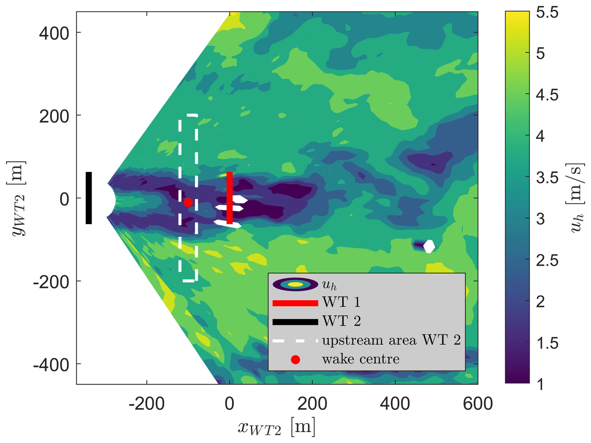
Figure 6 Wake centre identification from lidar measurements in a WT2-based coordinate system. The wind direction here is 205°, resulting in a partial wake constellation.

2.3.3 Uncertainty estimation

The uncertainty of the wake position y_w is subject to

• the lidar probe position uncertainty,

• the uncertainty in the horizontal wind speed at the probe position, when projected from the line-of-sight velocity, and

• the sensitivity of the wake centre identification method towards the wind speed uncertainty.

Schneemann et al., 2021Schneemann et al., 2021; Simley et al., 2020

Table 3 Uncertainties in the scope of the lidar data processing; values relate to the 95 % confidence interval for normally distributed uncertainties (i.e. a coverage factor of 2).

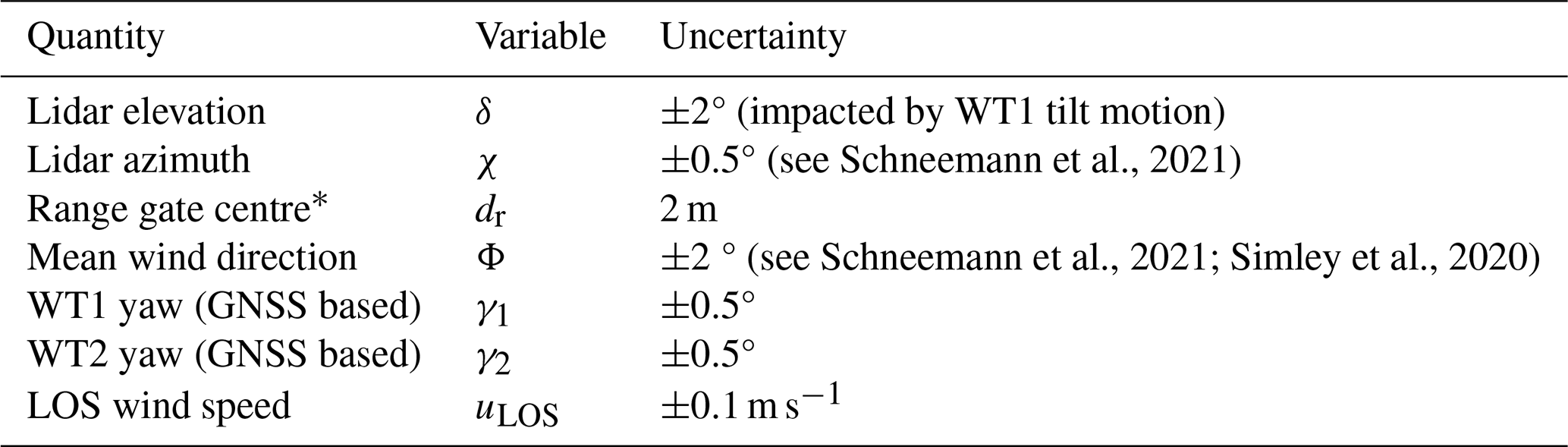
^∗ Range gate centre as a result of pulse length and time of travel; the range gate volume is considerably larger.

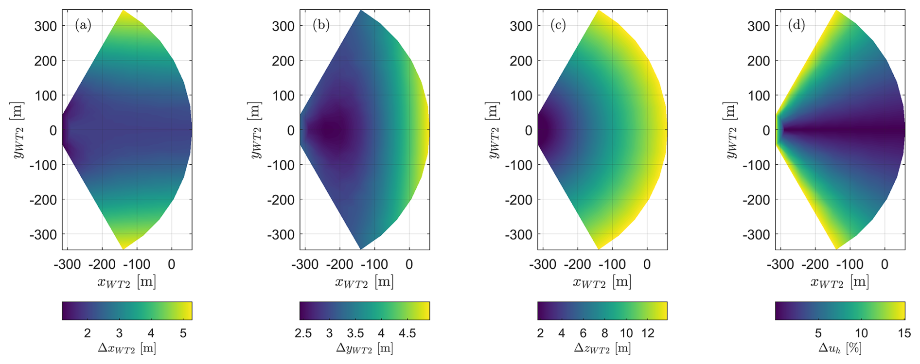
Figure 7 Illustration of uncertainty propagation: probe position uncertainty in x, y, and z, and horizontal wind speed uncertainty; WT2-based coordinate system.

In principle, an uncertain probe position could further influence the probed wind speed, for example when measuring at a different altitude than expected in a sheared or veered flow. This can be corrected for, as shown by Schneemann et al. (2021) for a long-range lidar experiment with range gates of multiple kilometres. In the work presented here, the probe position uncertainty is sufficiently small to neglect the effect of wind speed gradients at the probe position (see later in Fig. 7). The probe position is subject to the measurement uncertainties listed in Table 3. Their propagation through the coordinate transform in Eqs. (14)–(16) is formulated by Eq. (19), following the GUM standard (JCGM, 2020), where the expression (.)°² denotes the element-wise square operation for a vector. Also, the square root is to be understood element-wise. The uncertainties are illustrated in Fig. 7 for a full alignment case ($\mathrm{\Phi }={\mathit{\gamma }}_{\mathrm{1}}={\mathit{\gamma }}_{\mathrm{2}}=\mathrm{228}\mathit{°}$). Note that the uncertainties depend on the instantaneous constellation.

$$\begin{array}{}\text{(19)}& {\left[\begin{array}{c}\mathrm{\Delta }x\\ \mathrm{\Delta }y\\ \mathrm{\Delta }z\end{array}\right]}_{\mathrm{WT}\mathrm{2}}=\sqrt{\begin{array}{c}\left({\displaystyle \frac{\partial {\mathit{x}}_{\mathrm{WT}\mathrm{2}}}{\partial {\mathit{\gamma }}_{\mathrm{1}}}}\mathrm{\Delta }{\mathit{\gamma }}_{\mathrm{1}}\right){\mathit{°}}^{\mathrm{2}}+\left({\displaystyle \frac{\partial {\mathit{x}}_{\mathrm{WT}\mathrm{2}}}{\partial {\mathit{\gamma }}_{\mathrm{2}}}}\mathrm{\Delta }{\mathit{\gamma }}_{\mathrm{2}}\right){\mathit{°}}^{\mathrm{2}}+\\ \left({\displaystyle \frac{\partial {\mathit{x}}_{\mathrm{WT}\mathrm{2}}}{\partial \mathit{\delta }}}\mathrm{\Delta }\mathit{\delta }\right){\mathit{°}}^{\mathrm{2}}+\left({\displaystyle \frac{\partial {\mathit{x}}_{\mathrm{WT}\mathrm{2}}}{\partial \mathit{\chi }}}\mathrm{\Delta }\mathit{\chi }\right){\mathit{°}}^{\mathrm{2}}\end{array}}\end{array}$$

The uncertainty in the line-of-sight projection of the wind speed Δu_h can again be expressed considering the geometry:

$$\begin{array}{}\text{(20)}& \mathrm{\Delta }{u}_h=\sqrt{\begin{array}{c}{\left({\displaystyle \frac{\partial u_h}{\partial \mathit{\chi }}}\mathrm{\Delta }\mathit{\chi }\right)}^{\mathrm{2}}+{\left({\displaystyle \frac{\partial u_h}{\partial {\mathit{\gamma }}_{\mathrm{1}}}}\mathrm{\Delta }{\mathit{\gamma }}_{\mathrm{1}}\right)}^{\mathrm{2}}+{\left({\displaystyle \frac{\partial u_h}{\partial \mathrm{\Phi }}}\mathrm{\Delta }\mathrm{\Phi }\right)}^{\mathrm{2}}\\ +{\left({\displaystyle \frac{\partial u_h}{\partial \mathit{\delta }}}\mathrm{\Delta }\mathit{\delta }\right)}^{\mathrm{2}}+{\left({\displaystyle \frac{\partial u_h}{\partial u_{\mathrm{LOS}}}}\mathrm{\Delta }{u}_{\mathrm{LOS}}\right)}^{\mathrm{2}}\end{array}}.\end{array}$$

The impact of the wind speed uncertainty on the wake centre identification is investigated. If the wind speed uncertainties were randomly distributed along y_WT2, the convolution integral would hardly be affected, since it smoothes on a scale of 1D. However, it is more likely to have a wind speed uncertainty that is correlated along y_WT2, for example as the result of a misaligned lidar beam. This would promote wind speeds at one end of the probing area, while suppressing them at the other end. The bias would have a magnitude of ±5 % within the wake probing range, as visible in Fig. 7d. Figure 8 shows a normalized wake deficit example, which is corrupted by a linear bias of ±5 %. Applying the convolution method according to Eq. (18) yields a mis-assessment in the order of ±1 m (<0.01D) for all possible wake positions y_w. Note that this is no longer a standard uncertainty according to the GUM, since it contains the worst-case assumption of a linear bias. Also note that the mis-assessment of the method depends on the wake deficit. A less-pronounced wake deficit would have less impact in comparison to a correlated wind speed uncertainty. Qualitatively, the investigation showed the convolution method to be very robust and hardly affected by the expected range of wind speed uncertainty. The uncertainty of the probe y position and the wake centre identification uncertainty are subsequently added. The calculation is applied for each full lidar snapshot individually.

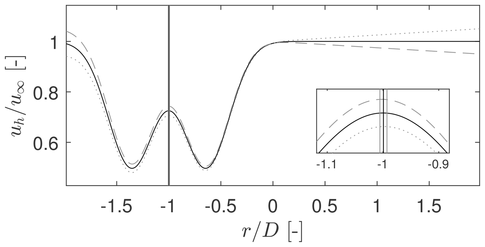
Figure 8 Example of convolution method to extract the wake centre position; impact of wind speed uncertainty on wake centre identification: generic double-Gaussian deficit as found in situ is distorted by two exemplary linear biases of ±5 %, which can be obtained from Fig. 7.

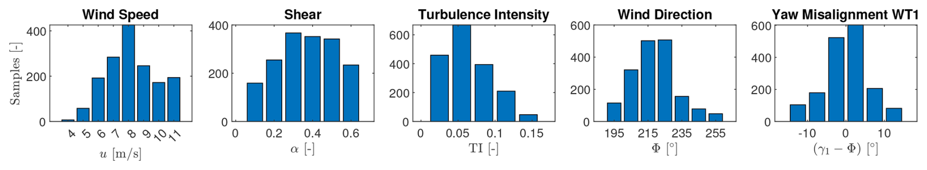
Figure 9 Histogram of ambient conditions contained in the investigated dataset; all measurements refer to the met mast (except for γ₁, which is probed via GNSS on WT1).

3 Results

In this section, the results of the field experiment and the wake estimation are reported. In Sect. 3.1, the wake conditions contained in the dataset are described, considering both the wake position variability and the wake deficit shape. In Sect. 3.2, the wake position estimates of the load-based EKF and the lidar are compared.

3.1 Wake condition characterization

This first part of the result section gives an overview of the wake conditions contained in the test data set. A histogram of the ambient conditions is shown in Fig. 9. In total, 1800 1 min samples (30 h) of wake constellations are contained. The wind speed distribution does not show the converged shape of a Weibull distribution yet, but the tendency is recognizable. A large share of high shear and low turbulence intensity is on hand, which is an indicator for very stable atmospheric conditions. Note here that atmospheric stability often follows diurnal cycles, while the dataset contains only data from 05:00 to 21:00 UTC, since the wind turbines often operated at a noise reduction mode during nighttime, which would not have been representative. Also note that the indicated yaw misalignment does not distinguish between intentional and unintentional yaw misalignment.

3.1.1 Wake position variability

In Fig. 10, the wake position y_w, as identified from the lidar scans, is plotted versus the wind direction. It shows higher spreading than suggested by the pure geometry, namely the turbine positions and the assumption of linear wake propagation parallel to the wind direction, indicated in red. The spreading has a magnitude of up to ≈ 40 m or 0.3D, which is considerably larger than the order of uncertainty connected with the wake centre identification, as discussed in Sect. 2.3.3. The spreading could originate from wake meandering, wind direction changes propagating through the test field, and wake steering control. The impact of the wake steering controller can be estimated by employing the analytical wake deflection model of Jiménez et al. (2009) or Larsen et al. (2020) and the available information of the yaw misalignment of WT1. These models give similar results, but the latter does not require any parameter fitting. Figure 10b shows results for the Jiménez model, which on average successfully encounters the direction and magnitude of wake deflections for the sector in which wake steering control was active (191–259°). Note that toggling between conventional and wake steering control was on hand, thus also many situations with no intentional yaw misalignment are contained in the plot. While the scattering range resulting from the Jiménez model is similar to the observed scattering seen in the lidar data, these scatters are not necessarily concurrent in time. Also, the double-sided deviations of the lidar-probed wake positions from the geometry line are not captured.

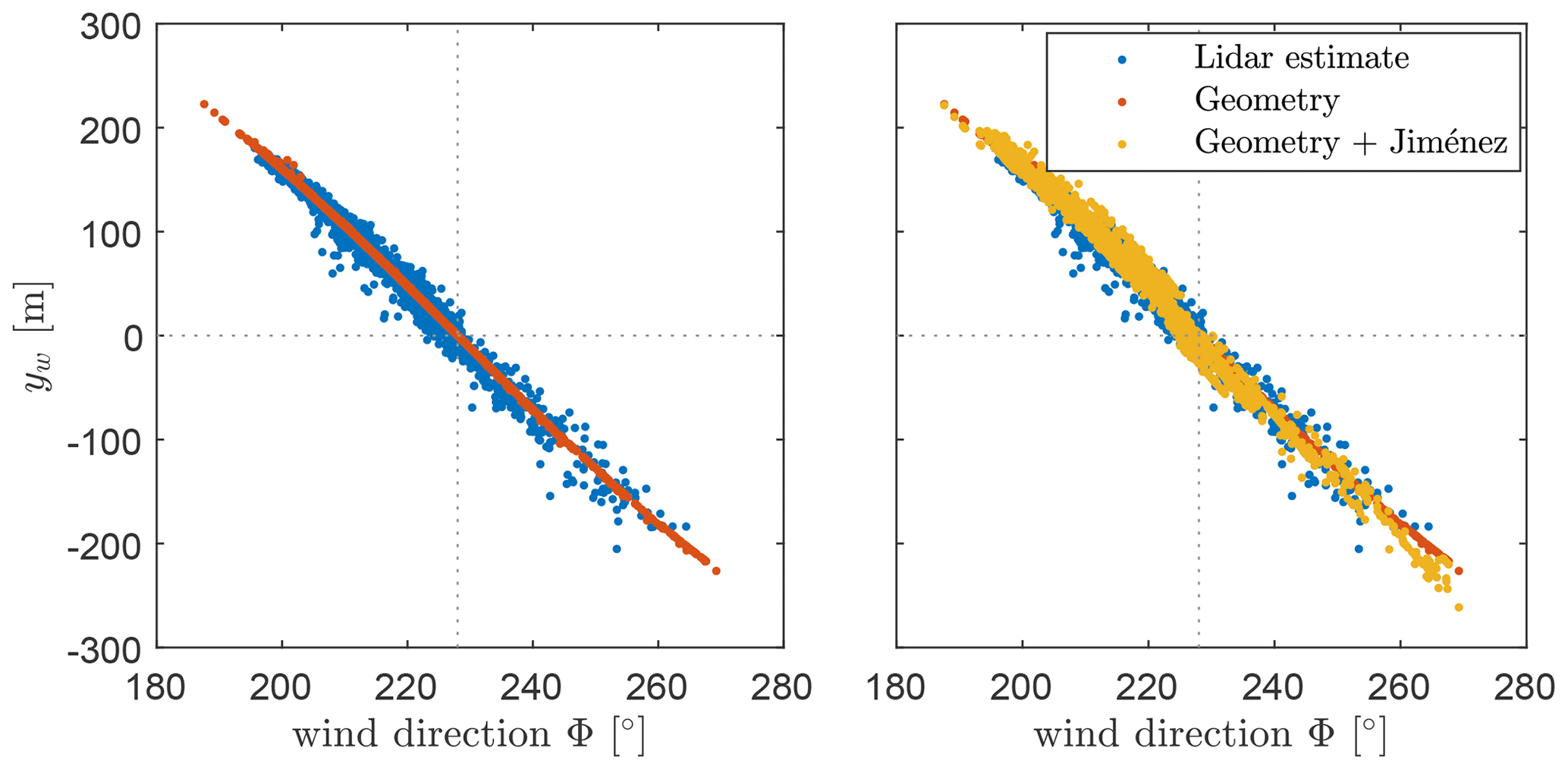
Figure 10 Wake centre position y_w in dependency of wind direction: Geometry denotes the pure consideration of farm geometry and linear wake propagation in the main wind direction, and Jimenéz denotes an analytic wake deflection model. Centre lines of zero deflection and full turbine alignment (228°) are marked.

3.1.2 Wake deficits

Figure 11 shows the wake deficits recorded by the lidar, superimposed within wind speed bins of 0.5 m s⁻¹. The instantaneous deficits are aligned along their identified wake centre, thus the horizontal axis in Fig. 11 is defined as $r=y_{\mathrm{WT}\mathrm{2}}-y_{\mathrm{w}}$ (compare Sect. 2.3.1). Each snapshot is plotted transparent, such that darker areas indicate higher occurrences of similar deficits. Some individual wake deficits differ considerably from the dominant bin average. The wake deficit shows the characteristic double-Gaussian shape of a near wake. Especially for larger wind speeds, a strong asymmetry is observed, pronouncing the wake at negative coordinates r (referring to the right side when facing downstream; compare Fig. 6).

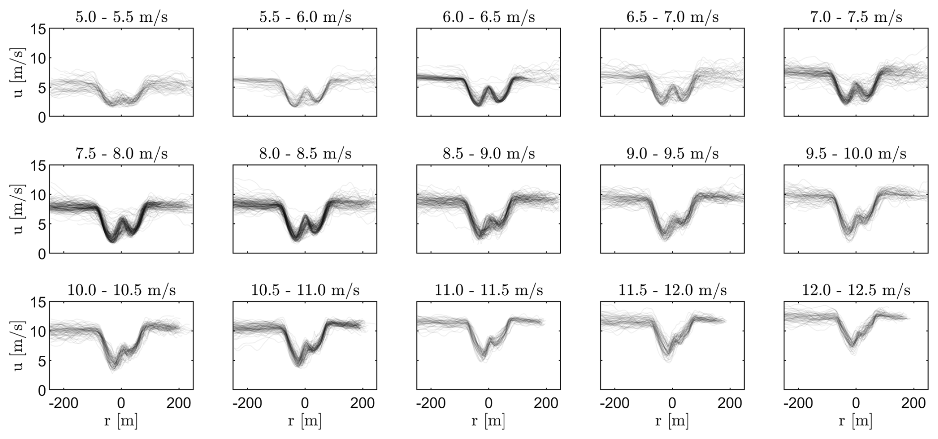
Figure 11 Spaghetti plot of the observed wake deficits per individual lidar scan, aligned along their identified wake centre, binned in steps of 0.5 m s⁻¹ and plotted transparent to visualize frequent occurrences of similar wake deficits.

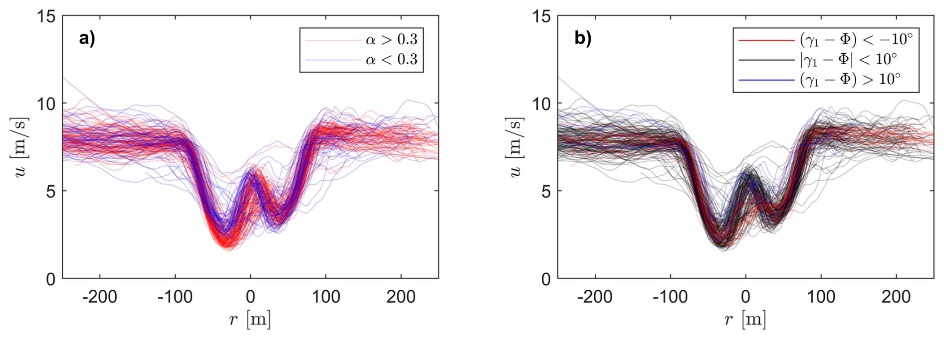
Figure 12 Wake deficits within wind speed bin 7.5–8 m s⁻¹: (a) colour coded for two ranges of shear profile, defined by power law coefficient α and (b) colour coded with respect to yaw misalignment of WT1.

The co-occurrence of the asymmetry with ambient conditions is documented in Fig. 12. A strong impact is visible when filtering for the power law coefficient α, describing the shear profile. Figure 12a indicates that the wake asymmetry is more pronounced at strong shear, connected to atmospheric stable conditions. For low shear coefficients, the wake deficits are rather symmetric. Larger wind speed variations among the deficits as well as in the non-waked area are on hand here, which again is attributed to the atmospheric stability. Figure 12b shows a distinction of wake deficits with respect to yaw misalignment situations, which are known to cause a kidney-shaped curled wake (see e.g. Bartl et al., 2018 and Sengers et al., 2023). While the main asymmetry of the double-Gaussian deficit – i.e. the magnitude difference of the two wake peaks – is linked to the ambient shear, a tendency towards a broader peak at the pronounced side of the wake is seen in the case of negative yaw misalignment. This finding is to be treated with care, since it is based on limited data availability (compare Fig. 9). The role of the wake deficit in this context is further discussed in Sect. 4.

3.2 Wake position estimates

This section shows the behaviour of the wake position estimation via load-based EKF and lidar recordings under various ambient conditions. Details are shown in a time series plot and lidar snapshots of the flow field, while the general performance is seized with bar plots of performance metrics applied on the entire dataset.

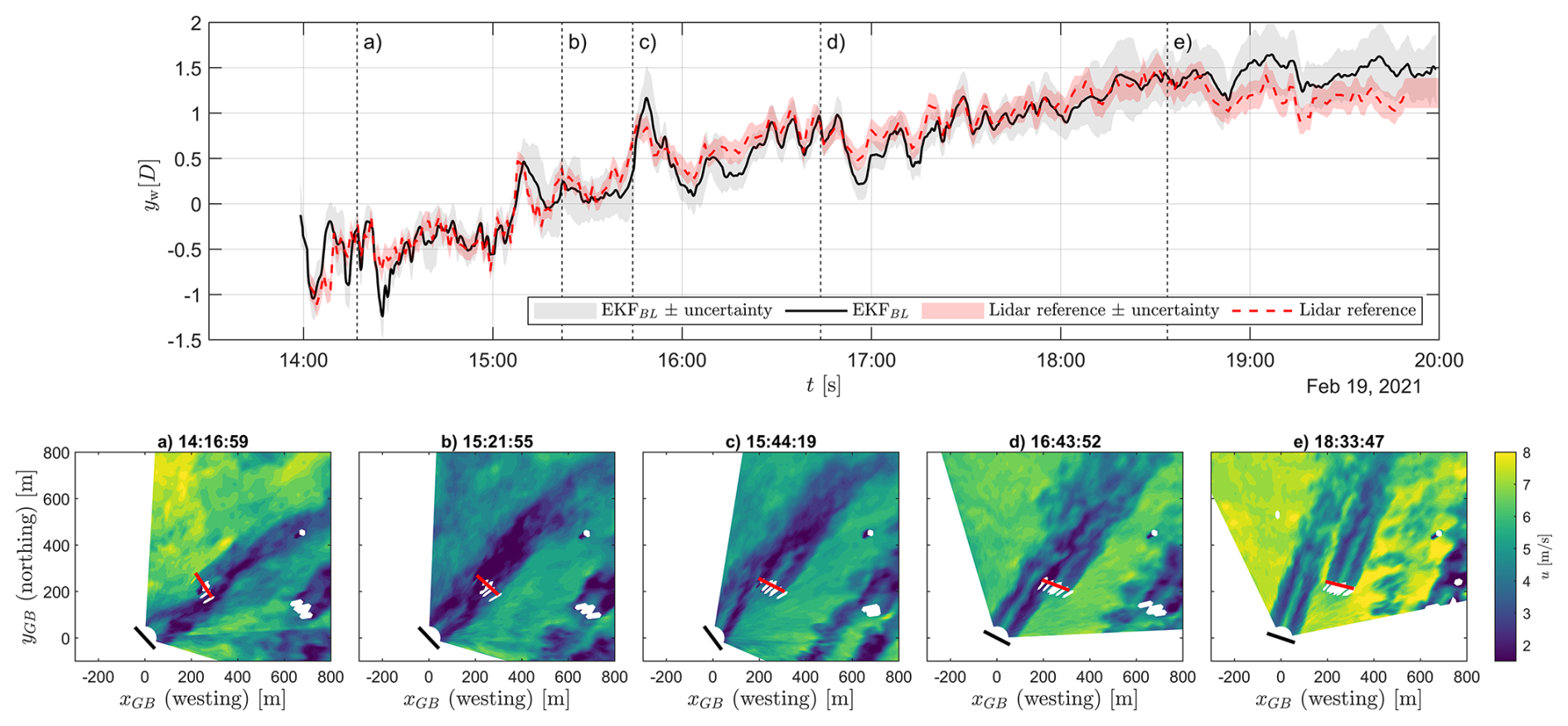
Figure 13 Top: time series of wake position estimate by load-based EKF and lidar; the uncertainty range for both methods is indicated. Bottom: snapshots of the instantaneous flow situation in the wind farm; ground-based coordinates are used. WT1 is indicated in black, WT2 in red. The time instances (a–e) refer to the indications in the time series plot on top.

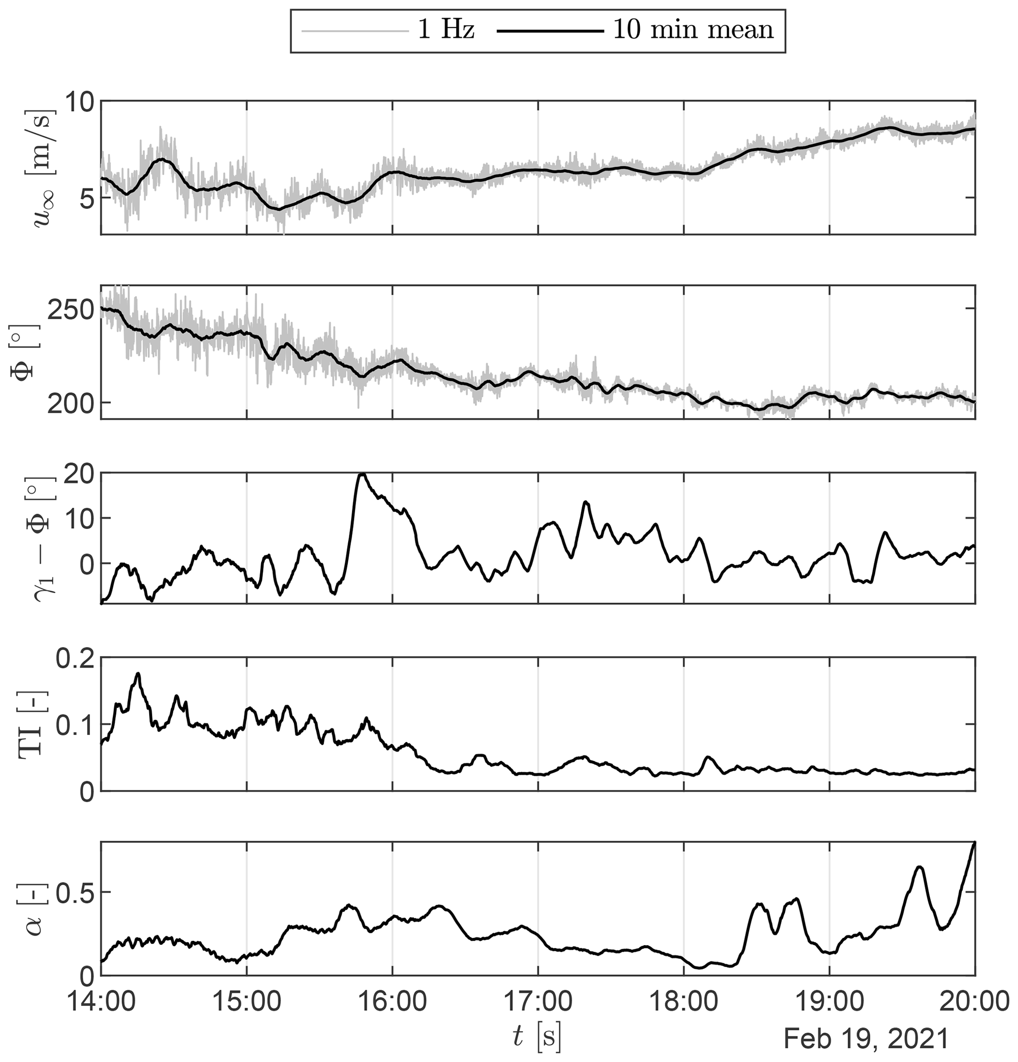
Figure 14 Ambient conditions on 19 February 2021, same time instance as shown in Fig. 13. Ambient wind speed u_∞ and wind direction Φ are shown as both 1 Hz and 10 min average. The TI refers to 10 min bins by definition, and the same was applied to power law coefficient α and WT1 yaw misalignment γ₁−Φ.

Figure 13 shows a 6 h wake position time series on 19 February 2021, including several lidar-recorded snapshots of the instantaneous flow situation in the wind farm. The corresponding ambient conditions as recorded by the nearby met mast are shown in Fig. 14. Within the shown time span, the wind direction changes from 250 to 200°, resulting in a full sweep of the wake across the rotor of WT2 (full alignment is at 228°). Constellations of partial wake, full wake, and barely impinging wake are covered. At the same time, the wind ramps up from 5 to 9 m s⁻¹. The atmospheric conditions change from unstable to stable, indicated by high TI, high wind direction variability and low α in the afternoon compared to low TI, and low wind direction variability and high α in the evening hours. The EKF is initialized at y_w=0 m and converges to the approximate wake position within approximately 2 min. Snapshots associated with a variety of conditions – labelled (a) to (e) – are analysed in detail.

• a.

  Partial wake (at 14:16 UTC): a wake constellation at $y_{\mathrm{w}}\approx -D/\mathrm{2}$, which agrees with the EKF estimate. The flow dynamics are high at this point in time, which can be seen in the position changes captured by the EKF as well as in the wind field.

• b.

  Full wake (at 15:21 UTC): while correctly identified by the EKF, the confidence interval of the EKF is slightly increased here. This is connected to decreased observability, a result of the flat gradient ${\left.\frac{\partial M_{col}}{\partial y_{\mathrm{w}}}\right|}_{y_{\mathrm{w}}\approx \mathrm{0}}$ used by the local linearization of the measurement model.

• c.

  Yaw misalignment (from 15:40 to 16:00 UTC): a high yaw misalignment (≈ 15°) of WT1 is present. The wake steering effect displays with a prominent wake position change, which is also visible in the flow situation of snapshot c. Both the lidar and the EKF capture the steep change in wake position in this time span.

• d.

  Meandering (16:30 and 16:50 UTC): The wake position oscillates several times between 0.5D and 1D. The time scales of these oscillations are around 300 s (referring to spatial scales of 14D at 6 m s⁻¹ ambient wind speed; compare Sect. 2.2.2). This is at the higher end of the dynamic range of the EKF, yet close to the transition between what is defined as meandering and as farm-effective wind direction variability.

• e.

  Barely impinging wake (from 18:00 to 18:40 UTC): The wind direction approaches 200°, and the average wake position moves from 1D to 1.5D, which leads to ceasing wake impingement. The loss of observability goes along with increased state covariance, thus a larger confidence interval of the EKF estimate. In the case of no wake impingement, the 2σ confidence is close to 0.5D for multiple time instances in a row (in the case of a single iteration increase, it could also mean a measurement outlier). The EKF position estimate stays approximately at the last known position but cannot be regarded as expressive here.

The EKF behaviour can further be assessed based on a spectra of the wake position time series, given in Fig. 15. The cut-off frequency of the EKF formulation f_c is indicated, which is also close to the band limit of the lidar scanning speed. Within 10⁻³ to 10⁻² Hz, the power spectral density (PSD) of EKF and lidar estimates is similar and decays with approximately −20 dB per decade. At higher frequencies, the EKF shows a trend of −40 dB per decade, where the additional attenuation is linked to the filter formulation. The filter also contributes to the rejection of changes in wake position faster than f_c, which might be suggested by higher-order load variations.

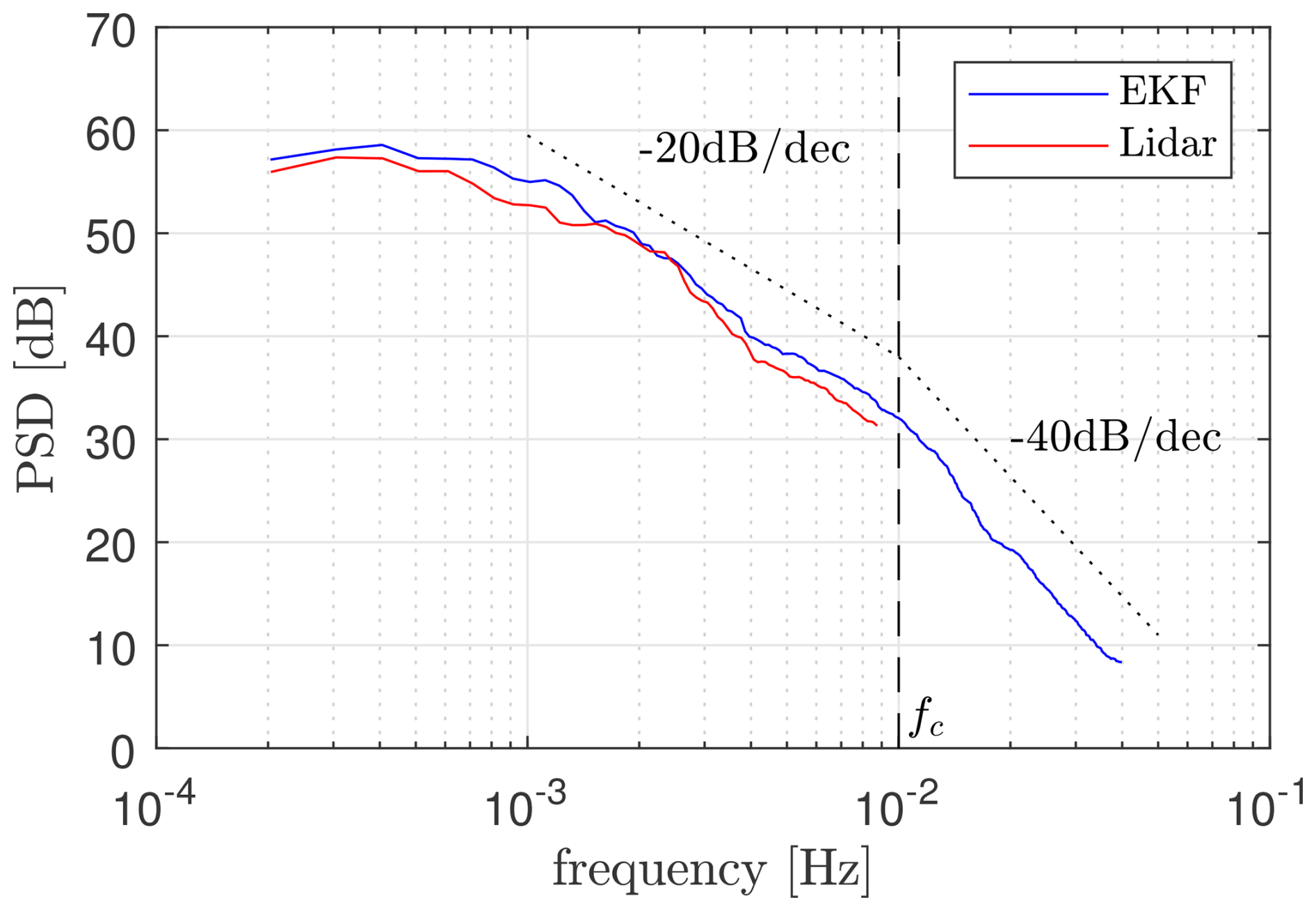
Figure 15 Power spectral density (PSD) of the wake position y_w, estimated by EKF and by lidar.

The performance of the entire test dataset is ranged with performance metrics. The estimates of lidar and EKF are compared with the root mean square error (RMSE), defined as

$$\begin{array}{}\text{(21)}& \mathrm{RMSE}=\sqrt{{\displaystyle \frac{\mathrm{1}}{N}}\sum _{k=\mathrm{1}}^N{\left(y_{\mathrm{w},k}^{\mathrm{EKF}}-y_{\mathrm{w},k}^{\mathrm{L}}\right)}^{\mathrm{2}}}.\end{array}$$

The RMSE does not capture the uncertainty consideration yet. The additional metric inRange is introduced in Eq. (22), denoting whether the estimates are within each other's 2σ uncertainty range. It further accounts for the fact that no ground truth exists. Instead, two uncertainty-containing signals are compared.

$$\begin{array}{}\text{(22)}& \mathit{inRange}={\displaystyle \frac{\mathrm{1}}{N}}\sum _{k=\mathrm{1}}^N{\mathrm{\Omega }}_k\end{array}$$

with

$${\mathrm{\Omega }}_k=\left\{\begin{array}{ll}\mathrm{1}& \left|y_{\mathrm{w},k}^{\mathrm{EKF}}-y_{\mathrm{w},k}^{\mathrm{L}}\right|<\mathrm{2}\sqrt{({\mathit{\sigma }}_k^{\mathrm{EKF}}{)}^{\mathrm{2}}+({\mathit{\sigma }}_k^{\mathrm{L}}{)}^{\mathrm{2}}}\\ \mathrm{0}& \mathrm{else}\end{array}\right.$$

The results are shown in Fig. 16, where binning with respect to the ambient conditions is applied, revealing the dependency on ambient wind speed, shear, TI and WT1 yaw misalignment. The share of data within the respective data bin is shown in Fig. 9, to allow the assessment of the results under consideration of the underlying statistical evidence. For example, the RMSE of a bin that contains only 3 % of the available data can be considered less expressive than a bin that represents 20 % of the dataset. The RMSE is generally around 0.2D and the inRange indicator around 90 %. No clear systematic dependency towards ambient wind speed and shear level is seen. The RMSE varies slightly among the bins, yet the inRange indicator is not notably affected. A trend for the turbulence intensity is visible, namely from 0.2D RMSE and inRange of 95 % at low TI to 0.3D RMSE and inRange of 75 % at high TI. The data availability decreases towards higher TI, yet the trend is persistent over all bins and for both metrics. At small yaw misalignments of WT1, the RMSE is lowest. Strong negative yaw misalignments seem to increase the RMSE. Yet, this finding is to be treated with care, since the data availability is comparably low here.

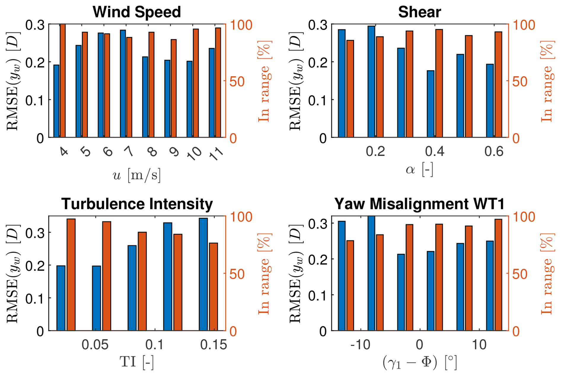
Figure 16 RMSE of wake position estimate (EKF vs lidar), binned with respect to the ambient conditions. The orange bars refer to the right y axis and represent the inRange indicator (i.e. whether the difference between the position estimates is covered by their uncertainty intervals).

4 Discussion

In this section, the results are interpreted and ranged. First, the influence of the site specifications on the results is discussed, considering the generalizability of the findings. Second, the wake tracking performance is discussed. The comparison to existing works in literature considers their individual testing conditions and performance metrics. Finally, the applicability of the presented wake tracking in the context of wind condition awareness and wind farm flow control is discussed.

4.1 Evaluation of the experimental conditions and data-processing methods

4.1.1 Site and wake conditions

The test site has very close spacing between the turbines, resulting in a near wake with a characteristic double-Gaussian deficit shape. The consequence for the estimation task is twofold. On the one hand, the wind speed deficit is very pronounced, so it leaves a considerable footprint on the rotor of a subsequent turbine. On the other hand, a double-Gaussian wake deficit is a more complex structure, thus requiring higher degrees of freedom for its description in comparison to a single-Gaussian (Keane et al., 2016). The scanning lidar can resolve this, and even an EKF-based four fixed-beam staring lidar approach as described by Lio et al. (2021) shows sufficient observability. Existing works on estimation using turbine measurements either do not consider near-wake features (Doekemeijer and van Wingerden, 2020; Cacciola et al., 2016) or assume a quasi-steady wake velocity deficit to be known a priori (Dong et al., 2021). The latter is similar to this work, where the wake deficit is implicitly contained in the training data. Even more complexity is added due to the occasional wake asymmetry, reported in the context of Fig. 11. The wake asymmetry is found to dominantly co-occur with strong wind shear and to increase with ambient wind speed, and thus also rotational speed. An interaction of wake rotation and the sheared flow is assumed. The rotational component in the wake flow, in opposite direction to the rotor rotation, could cause an “upwash” of wind speeds from low altitudes on the right side of the rotor (facing downstream, thus negative on the y axis) and a “downwash” of wind speeds from higher altitudes on the left side. The direction of wake rotation and the observed orientation of the wake asymmetry would support this explanation. A comparable near-wake asymmetry is reported by Bromm et al. (2018) in a similar field campaign. A minor co-occurrence of wake asymmetry and large WT1 yaw misalignments (> 10°) is found, matching the expectation with regard to the curled wake phenomena (Bartl et al., 2018; Sengers et al., 2023). Yet, data availability of large yaw misalignments is not considered sufficient to draw a clear conclusion on curled wakes, which are also not a focus of this work.

Another consequence of small downstream distance is a low meandering amplitude (Machefaux et al., 2015). It is expected that the load-based EKF would have been able to capture higher meandering amplitudes, as shown in a wind tunnel experiment with tailored meandering wake conditions (Onnen et al., 2023). In the given field setup, however, a considerable share of the involved wake position dynamics can be accounted for in wind direction changes and active yaw control.

4.1.2 Uncertainty

The uncertainty consideration for the lidar estimate is deliberately chosen to be mainly based on analytical error propagation rather than on statistical approaches. On the one hand, this choice enables the user to identify and unravel the impact of individual quantities' contributions to the combined uncertainty of the processed wake position. In this case, the wind speed uncertainty shows negligible impact when locating a coherent flow structure. The major contributions originate from the propagation of geometric uncertainties. These can be limited with adequately precise measurement equipment, such as the GNSS encoders for the nacelle yaw probing used in this setup. On the other hand, the uncertainty is available for every time instance independently, thus not depending on the dataset size, as would be the case for a statistically derived uncertainty. The lidar estimate generally has a combined 2σ uncertainty below 0.06D, which makes it a suitable reference in comparison to the difference between the lidar- and the load-based method, which is at the order of 0.2D (RMSE). Trujillo (2017) names 0.05D as the accuracy of lidar-based wake position extraction at short downstream distances, which is very similar to this work. The uncertainty of the EKF estimate is directly taken from its state covariance matrix (Eichstadt et al., 2016). The involved linearization of the measurement model is similar to the 1st-order approximations used for analytic error propagation.

4.2 Wake tracking performance

In contrast to a simulation study, a pure performance assessment of one wake tracking methodology is not possible in a field experiment, since no ground truth exists as reference. Instead, two uncertainty-containing estimates from two different methods are compared. The wake position estimated with the scanning lidar can be regarded as an attempt to provide a reference value closer to a virtual ground truth.

4.2.1 Impact of ambient conditions

The match between lidar- and load-based position estimates shows no clear dependency on the ambient wind speed. Small variations among the bins could originate from a limited dataset size, which might not equal out coinciding instances of certain wind speeds with for example certain turbulence intensities. An indication for a not fully converged dataset is the wind speed histogram in Fig. 9, showing that the occurring wind speeds do not fully represent the shape of a Weibull distribution. In a simulation study, no direct impact of the ambient wind speed on the estimation is reported, as long as both the wake-causing turbine and the estimating turbine are not operating at the transition of partial to full load range (Onnen et al., 2022).

The observed increase of RMSE with TI is expected and agrees with simulation studies of load-based estimation (Dong et al., 2021; Onnen et al., 2022) and field results of lidar-based wake estimation (Lio et al., 2021). Higher turbulence intensities affect both the shape of the instantaneous wake deficit and the dynamics of the wake position. The information contained in the blade root loads is typically not sufficient to distinguish between both aspects, especially when their characteristic time scales are overlapping. The definition of the cut-off frequency in the dynamic model of the EKF leads to a rejection of turbulent scales smaller than the rotor scale. Deviations of the wake deficit shape that persist at scales of multiple rotor diameters could be misinterpreted as a change in wake position. This holds for the method described in this work, where wake deficit information is indirectly contained in the training data, as well as for methods that aim to estimate the wake deficit online, yet on slow time scales (Lio et al., 2021). The relation between the instantaneous wake deficit and the wake centre position further impacts the respective definitions of the wake centre: the convolution with density of available power (as applied on the lidar data; compare Sect. 2.3.2) always considers the entire wake deficit. In case of non-symmetry, it identifies its centre with a shift towards the more pronounced side of the wake deficit. The load-based method, however, solely judges the share of the deficit which overlaps with the estimating turbine.

An impact of the wind shear on of the tracking performance could have been expected, as the asymmetry of the wake deficit shows to be influenced. However, the low shears often coincide with high TI, both as features of atmospheric instability. It is not possible to fully isolate the effects from shear and TI, and although the wake asymmetry due to high shears would lead us to expect a worse tracking performance, this was not observed.

4.2.2 Comparison to other wake estimation methods

The comparison to other existing methods considers the respective performance metrics, the test environment (simulations, wind tunnel, or field), and the underlying methods and assumptions. Cacciola et al. (2016) show static inaccuracies of 0.1–0.2D for the determination of the wake centre position at TI = 5 %, 10 % in aeroelastic simulations. Each position estimate is based on 10 min averaging and a least-squares fit of rotor-effective horizontal shear with respect to the rotor loads. Bottasso et al. (2018) show detection ratios per location interval (discretized with 0.25D) as a performance measure. The detection method compares the difference in EKF-estimated sector-effective wind speeds with a threshold, which again is subject to scheduling with the ambient conditions. It is also tested in an aeroelastic environment, both in static wake conditions and in a scenario where a single-Gaussian wake deficit follows a sine trajectory at a frequency of $f\approx u_{\mathrm{\infty }}/\left(\mathrm{2}D\right)$. The simulations allow for a ground truth reference, but other than that, the detection ratio is similar to the inRange metric used in this paper. Bottasso et al. (2018) show a detection ratio close to 100 % for static wakes and 5 % TI, which decreases to approximately 75 %–80 % at 10 % TI. This is similar to the results reported in Fig. 16. The works also agree that ambient shear decreases the accuracy, while estimation is still possible under moderate yaw misalignment of the tracking turbine. At full wake constellations, the method of Bottasso et al. (2018) has no observability, because the wake-induced rotor loads are not asymmetric. Here, the comparison between the methods lacks, because they do not use the undisturbed wind speed. But, as also pointed out by the authors, the blind spot at full wake could be avoided when comparing the ambient wind speed with the rotor-effective wind speed or redundantly with the collective blade loads, as done in this paper. Onnen et al. (2022) test a nearly identical EKF formulation as in this work with aeroelastic simulations using the DWM model and the DTU 10 MW turbine. The RMSE of 0.05D, 0.1D, and 0.2D is found for turbulence intensities of 5 %, 10 %, and 15 %, respectively. A similar RMSE is shown in another aeroelastic study by Dong et al. (2021), with a similar load-based EKF. In general, the field test shows increased RMSE in comparison to the simulation tests, which can likely be attributed to the more uncertain environment. The qualitative tracking ability, as quantified with the detection ratio or inRange indicator is not notably impacted.

Wind tunnel results with two model turbines of 2 m diameter are shown by Schreiber et al. (2016). The methodology is similar to the one of Cacciola et al. (2016), and a time averaging of 1 min is used, which corresponds to approximately 1 h in the field, considering the scaling. Static inaccuracies of 0.1–0.2D are found in sheared inflow and 8 % TI. Dynamic wind tunnel tests are shown by Onnen et al. (2023), where a 1.8 m model turbine is exposed to wake conditions tailored with an active grid. The estimation accuracy is below 0.1D (RMSE). This is considerable lower than in the field tests shown here, most likely due to the controlled environment, a low ambient TI, and no wind direction variability.

To the authors' knowledge, the only field test of load-based wake estimation is reported by Schreiber et al. (2020). Qualitative wake impingement detection (left/right/full wake) is successfully shown, where the farm layout and the assumption of wake propagation parallel to the met mast wind direction serve as a reference. The availability of a scanning lidar in this work allows for a quantitative assessment while probing with higher spatial and temporal resolution. Further field experiments with scanning lidar-based wake position identification are reported by Bromm et al. (2018), where a propagated uncertainty of 0.05–0.1D is stated, similar to this work. Lio et al. (2021) show wake position tracking with simultaneous estimation of the deficit shape and shear profile. It is based on a few-beam staring lidar and an EKF considering the wake meandering dynamics. An RMSE of 0.05D, 0.12D, and 0.18D is shown, for 5 %, 10 %, and 15 % TI respectively. In their work, the reference is a 1 Hz least-squares fit of a parameterized deficit to 178-point scans by three synchronized lidar WindScanners. The tracking is slightly more precise than in this work, while Lio's method is based on different inputs and requires less external information.

4.3 Applicability

Load- and lidar-based wake estimation techniques have different outlooks for application. While lidars are still in the early industrial adaption phase, load-based approaches can be a reliable alternative and implemented solely using the standard sensors of modern wind turbines. This comes at the cost of slightly reduced observability or dependency on external information. The accuracy of the load-based tracking also needs to be ranged in relation to the expected magnitude of wake deflections due to wake steering control. At very short turbine spacing, such as in this experiment, the uncertainty of the EKF estimate is close to the expected magnitude of wake deflections (Jiménez et al., 2009). The conclusion is that purely using the wake position as closed-loop feedback is too narrow a consideration. Still, this paper shows that satisfying wake estimation with the ability to support robust closed-loop wake steering with suitable feedback information of high spatial and temporal resolution is possible. The time resolution helps especially when not only considering the absolute wake position estimate (which might e.g. be corrupted by an aberrated wake deficit) but also the change in wake position, which can be the intended response to a wake-steering manoeuvre. The required knowledge of the ambient conditions can arguably be estimated by a front row wind turbine (Soltani et al., 2013). Wake steering is, contrary to active wake control using a de-rating strategy, mostly applicable in low-turbulent stable situations. This is also where the methodology shows best performance in the field, in agreement with expectations according to simulations.

This paper focuses on the wake position as an exemplary aspect of wind condition awareness. A similar dataset and processing chain could also be used to validate wind farm models or wind field reconstruction based on in situ probings. Future work will be to embed sensor-based estimation within dynamic wind farm models (Becker et al., 2022; Lejeune et al., 2022), thus to couple analytic models, for example for the wake deficit or wake deflection. The relevance of open-loop approaches in wind farm flow control persists, since the impact of every control action is delayed by the advection duration of wakes. Closed-loop yaw control does not necessarily need to happen at very fast time scales, where its effect could overlap with those of wake meandering. State estimation could also support as a feedback, whether the open-loop models predict as expected or if (online) re-calibration is necessary (see Hulsman et al., 2024). Furthermore, the estimation of wake constellations yields information on the farm-effective wind direction. It can complement error-prone and point-probing nacelle vane signals and thus contribute to a consensus-based farm-effective wind direction (Annoni et al., 2019).

5 Conclusions

The paper presents a quantitative field comparison of two independently applied wake centre estimation methods: a nacelle-based scanning lidar and an EKF based on rotor loads. The methodology accounts for the fact that there is no ground truth in the field by a detailed uncertainty evaluation. The lidar estimates have an uncertainty in the order of 0.05D, which is a suitably precise reference to draw conclusions regarding the load-based EKF. It is a step forward in spatial resolution in comparison to the assumption of wake propagation parallel to the main wind direction. Both tracking methods agree with an RMSE of 0.2D for low to moderate TI, while increasing to 0.3D for a TI above 12 %. The EKF formulation further yields the uncertainty of the state estimate as a by-product, thus it self-indicates how certain or “observable” a situation is. Insights on the full flow field with the lidar allow the user to identify the observability limits of the load-based EKF, for example to distinguish between the influence of exact wake shape and the wake centre position. Due to close turbine spacing and frequent high-shear conditions, the observed wake deficits in this work are rather complex, mainly double-Gaussian, often asymmetric, and thus also influencing the wake centre definition. Yet, the methodology shows consistent behaviour even under these circumstances, which gives rise to the expectation that it would work similarly well or even better in settings with single-Gaussian wakes, although the wake load footprints are relative weaker under such circumstances. While this paper focuses on the wake position as one aspect of wind condition awareness, it also outlines how wind farm models or turbine-based wind field reconstruction can be validated with complementary lidar data.

Appendix A: Determination of rotor angle via edgewise blade root loads

The rotor angle of WT2 was not available to the authors. It was reconstructed from the edgewise blade root bending moments M_e. The method is based on the assumption that gravity is the main force contributing to the variation of the edgewise blade root bending moment (RBM). Let Ψ be the rotor angle, which is defined as positive clockwise and zero for blade 1 pointing upwards. Accordingly, each blade's edgewise RBM is modelled as

$$\begin{array}{}\text{(A1)}& \begin{array}{rl}& M_{\mathrm{e},\mathrm{1}}={\widehat{M}}_{\mathrm{e}}\sin \left(\mathrm{\Psi }\right)+{\stackrel{\mathrm{‾}}{M}}_{\mathrm{e}}\\ & M_{\mathrm{e},\mathrm{2}}={\widehat{M}}_{\mathrm{e}}\sin \left(\mathrm{\Psi }+{\displaystyle \frac{\mathrm{2}\mathit{\pi }}{\mathrm{3}}}\right)+\stackrel{\mathrm{‾}}{M_{\mathrm{e}}}\\ & M_{\mathrm{e},\mathrm{3}}={\widehat{M}}_{\mathrm{e}}\sin \left(\mathrm{\Psi }+{\displaystyle \frac{\mathrm{4}\mathit{\pi }}{\mathrm{3}}}\right)+\stackrel{\mathrm{‾}}{M_{\mathrm{e}}},\end{array}\end{array}$$

where ${\widehat{M}}_{\mathrm{e}}$ is the amplitude and $\stackrel{\mathrm{‾}}{M_{\mathrm{e}}}$ is a non-oscillating offset, connected to the rotor torque. Using the addition theorem of the sine function

$$\begin{array}{}\text{(A2)}& \sin (a+b)=\sin \left(a\right)\cos \left(b\right)+\sin \left(b\right)\cos \left(a\right),\end{array}$$

this can be reformulated as

$$\begin{array}{}\text{(A3)}& \begin{array}{rl}& \left[\begin{array}{c}{M}_{\mathrm{e},\mathrm{1}}\\ M_{\mathrm{e},\mathrm{2}}\\ M_{\mathrm{e},\mathrm{3}}\end{array}\right]=\left[\begin{array}{ccc}\mathrm{1}& \mathrm{0}& \mathrm{1}\\ -\frac{\mathrm{1}}{\mathrm{2}}& \frac{\sqrt{\mathrm{3}}}{\mathrm{2}}& \mathrm{1}\\ -\frac{\mathrm{1}}{\mathrm{2}}& -\frac{\sqrt{\mathrm{3}}}{\mathrm{2}}& \mathrm{1}\end{array}\right]\left[\begin{array}{c}{\widehat{M}}_{\mathrm{e}}\sin \left(\mathrm{\Psi }\right)\\ {\widehat{M}}_{\mathrm{e}}\cos \left(\mathrm{\Psi }\right)\\ \stackrel{\mathrm{‾}}{M_{\mathrm{e}}}\end{array}\right]\\ & \iff \left[\begin{array}{c}{\widehat{M}}_{\mathrm{e}}\sin \left(\mathrm{\Psi }\right)\\ {\widehat{M}}_{\mathrm{e}}\cos \left(\mathrm{\Psi }\right)\\ \stackrel{\mathrm{‾}}{M_{\mathrm{e}}}\end{array}\right]={\left[\begin{array}{ccc}\mathrm{1}& \mathrm{0}& \mathrm{1}\\ -\frac{\mathrm{1}}{\mathrm{2}}& \frac{\sqrt{\mathrm{3}}}{\mathrm{2}}& \mathrm{1}\\ -\frac{\mathrm{1}}{\mathrm{2}}& -\frac{\sqrt{\mathrm{3}}}{\mathrm{2}}& \mathrm{1}\end{array}\right]}^{-\mathrm{1}}\left[\begin{array}{c}{M}_{\mathrm{e},\mathrm{1}}\\ M_{\mathrm{e},\mathrm{2}}\\ M_{\mathrm{e},\mathrm{3}}\end{array}\right].\end{array}\end{array}$$

The rotor angle is calculated as

$$\begin{array}{}\text{(A4)}& \mathrm{\Psi }=\mathrm{atan}\left({\displaystyle \frac{{\widehat{M}}_{\mathrm{e}}\sin \left(\mathrm{\Psi }\right)}{{\widehat{M}}_{\mathrm{e}}\cos \left(\mathrm{\Psi }\right)}}\right).\end{array}$$

To mitigate the impact of the blade loads not behaving purely harmonic, for example due to tower shadow and non-uniform inflow, the nominator and denominator in Eq. (A4) are filtered with a zero-phase low-pass filter. The filtering at this point avoids filtering a non-continuous angle signal. The resulting determination of the rotor angle is shown for field data in Fig. A1 and shows the expected behaviour. The method was additionally validated with the aeroelastic model of the turbine in openFAST, where the rotor angle is available.

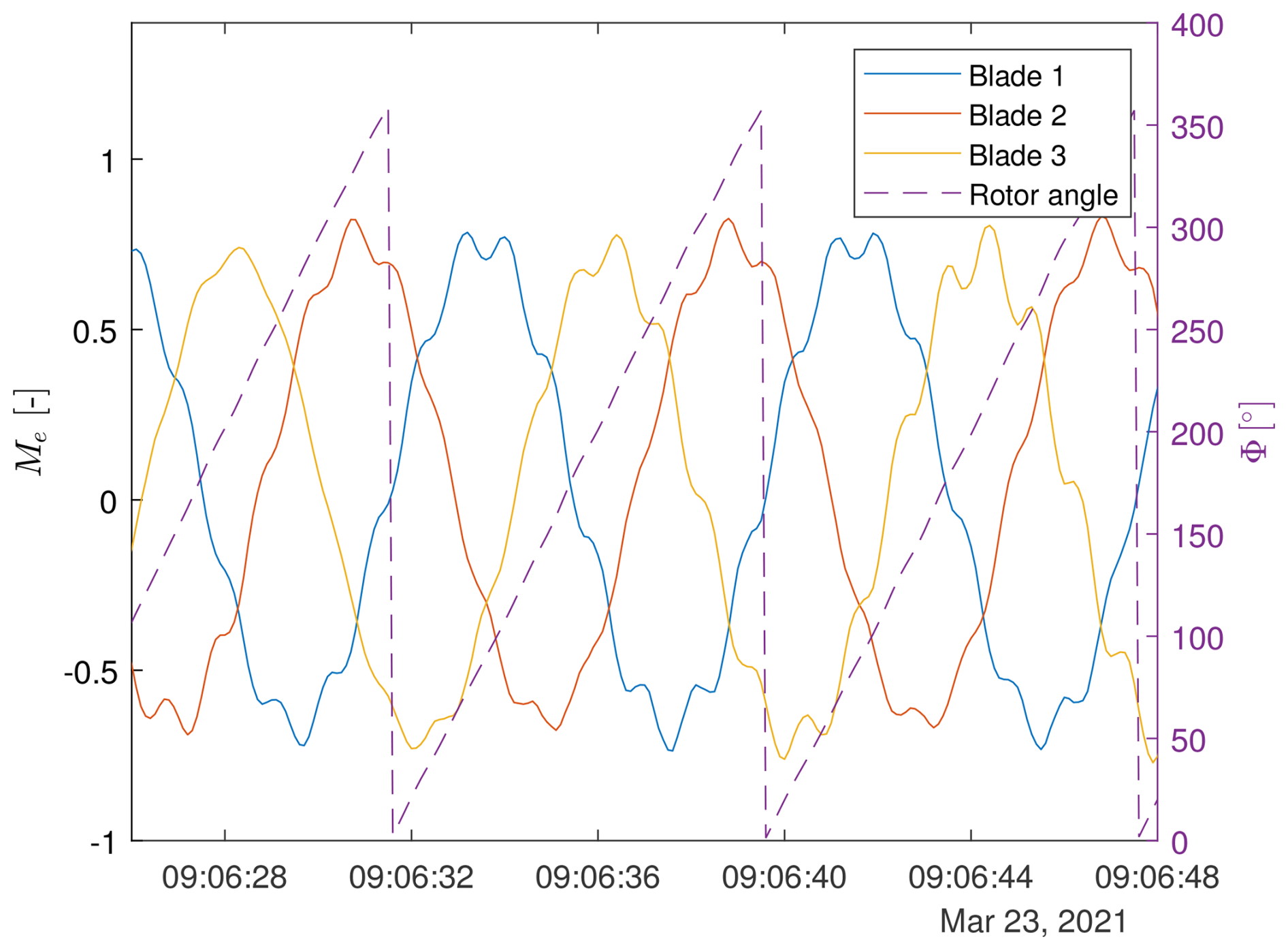
Figure A1 Identification of the rotor angle (on right y axis) from edgewise blade loads (on left y axis); loads were non-dimensionalized for confidential reasons.